Malaria detection using Deep Convolution Neural Network

I Abstract

The latest WHO report showed that the number of malaria cases climbed to 219 million last year, two million higher than last year. The global efforts to fight malaria have hit a plateau and the most significant underlying reason is international funding has declined. Malaria, which is spread to people through the bites of infected female mosquitoes, occurs in 91 countries but about 90% of the cases and deaths are in sub-Saharan Africa. The disease killed 4,35,000 people last year, the majority of them children under five in Africa. AI-backed technology has revolutionized malaria detection in some regions of Africa and the future impact of such work can be revolutionary. The malaria Cell Image Data-set is taken from the official NIH Website NIH data. The aim of the collection of the dataset was to reduce the burden for microscopists in resource-constrained regions and improve diagnostic accuracy using an AI-based algorithm to detect and segment the red blood cells. The goal of this work is to show that the state of the art accuracy can be obtained even by using $2$ layer convolution network and show a new baseline in Malaria detection efforts using AI.

II Introduction

In the engineering , model-based design[1], model based control[2], and model based optimization[3] are the essential components. The discovery of new data-driven models especially deep convolution neural networks in recent times that have worked well in image classification (AlexNet[4] ), engineering design[5], autonomous driving car[6, 7], radiology [8], human genome[9], and many more for developing state of the art[7] control and prediction systems are revolutionizing. Convolution Neural Networks (CNN) are said to be inspired by biological processes that take place in the human brain and the connectivity pattern between neurons resembles the organization of the animal visual cortex. The convolutional layer is the core building block of a CNN. The layer’s parameters consist of a set of learnable filters also called kernels, the parameters of the kernel are trained during the learning process and used during prediction. In 2012, a CNN called AlexNet[4] won the ImageNet Large Scale Visual Recognition Challenge. In later years, GoogLeNet[10] increased the mean average precision of object detection to 0.439329, and reduced classification error to 0.06656, the best result to date. The performance of GoogLeNet was close to or more than that of humans. In this work, the goal is to use the CNN-based network in the classification of cell images to distinguish between parasitized and uninfected cell images. We found that a small network can work better than the current state of art network done so far on Malaria detection if the hyperparameter is tuned properly. The expected benefit of the small network is the deployment of a malaria detection system on resource-constrained devices like mobile phones and tablets where high-performance computing is not available in those regions.

III The problem

The most widely used method (so far) is examining thin blood smears under a microscope, and visually searching for infected cells. The patient’s blood is smeared on a glass slide and stained with contrasting agents to better identify infected parasites in their red blood cells. Then, a clinician manually counts the number of parasitic red blood cells, sometimes up to 5,000 cells (according to WHO protocol). Manually counting is error-prone and slow. A clinician takes 10 minutes to 30 minutes to count such a number as it is a time-consuming process. There are general guidelines that lab technicians should process no more than 25 slides each day, but a lack of qualified workers leads some to process four times as many.

Why a neural network? Neural networks have performed really well in recent years in their ability to automatically extract features and learn filters and acted as a very good classifier of images. In previous machine learning solutions, features had to be manually programmed in, for example, size, color, and the morphology of the cells. Utilizing convolutional neural networks (CNN) will greatly speed up prediction time while mirroring (or even exceeding) the accuracy of clinicians.

Dataset: Data is the basic building block of CNN-based predictor. Without data, the training of the network is not possible. Thankfully, we have a labeled and preprocessed dataset of cell images to train and evaluate our model. NIH[11] has a malaria dataset of 27,558 cell images with an equal number of parasitized and uninfected cells. Datasets contains 2 folders:$1$ Infected ; $2$ Uninfected. This total $27,558$ images are of variable size color images with equal instances of parasitized and uninfected cells from the thin blood smear slide images from the Malaria Screener research activity. Giemsa-stained thin blood smear slides from 150 patients, falciparum-infected and 50 healthy patients were collected and photographed at Chittagong Medical College Hospital, Bangladesh. The smartphone’s built-in camera acquired images of slides for each microscopic field of view. The images were manually annotated by an expert slide reader at the Mahidol-Oxford Tropical Medicine Research Unit in Bangkok, Thailand.

IV Approach

Classification of cell images is an interesting problem and has great utility. There are already country and medical universities which are leveraging this AI-backed technology that can detect diseases(refer to related works). I choose LeNet5[12] as the starting model, which can work with grayscale images. The Le-Net5 network is modified for multi-channel images (as images are on RGB scale) to work with 3 layers of images. and further hyperparameter tuning[13] is done to classify colored cell images with an efficiency target of 95% or more on the test data set.

A deep convolution neural network uses an algorithm with millions of pictures as input to train before it is able to generalize the input and make predictions for images it has never seen before. To teach an algorithm how to recognize objects in images, we use a specific type of Artificial Neural Network: a Convolutional Neural Network (CNN). Their name stems from one of the most important operations in the network: convolution. Convolutional Neural Networks are inspired by the brain. Research in the 1950s and 1960s by D.H Hubel and T.N Wiesel on the brain of mammals suggested a new model for how mammals perceive the world visually. They showed that cat and monkey visual cortexes include neurons that exclusively respond to neurons in their direct environment. The computer world consists of only numbers. Every image can be represented as multi-dimensional arrays of numbers, known as pixels. CNNs, like neural networks, are made up of neurons with learnable weights and biases. Each neuron receives several inputs, takes a weighted sum over them, passes it through an activation function, and responds with an output. The whole network has a loss function. Unlike feed-forward neural networks, where the input is a vector, where the input is a multi-channeled image (3 channel in this case). The convolution layer is the main building block of a convolutional neural network. The convolution layer comprises a set of independent filters. Each filter is independently convolved with the image and we end up with multi-layer feature maps. All these filters are initialized randomly and become our parameters which will be learned by the network subsequently. Parameter sharing is sharing of weights by all neurons in a particular feature map. Local connectivity is the concept of each neural connected only to a subset of the input image (unlike a neural network where all the neurons are fully connected) This helps to reduce the number of parameters in the whole system and makes the computation more efficient. A pooling layer is another building block of a CNN. Its function is to progressively reduce the spatial size of the representation to reduce the number of parameters and computations in the network. The pooling layer operates on each feature map independently. Batch normalization is a method we can use to normalize the inputs of each layer, in order to fight the internal covariate shift problem. During training time, a batch normalization layer does the following: it first calculate the mean and variance of the layer’s input, then it normalizes the layer inputs using the previously calculated batch statistics, and last, it scales and shifts in order to obtain the output of the layer. Dropout is a regularization technique for neural network models. Dropout technique randomly selected neurons are ignored during training. They are “dropped out” randomly. This means that their contribution to the activation of downstream neurons is temporally removed on the forward pass and any weight updates are not applied to the neuron on the backward pass.

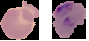
Data: The data set was downloaded from the NIH website[11]. A sample of image for both ’not infected cell’ and ’infected cell’ is shown below. On the left, we have a cell image, which is not infected by the malaria parasite. The infected cell image contains violet dots, which represent the malaria plasmodium parasite during imaging.

Figure 1: Input data image of cell (left : Not infected cell) ; (right : Infected cell)

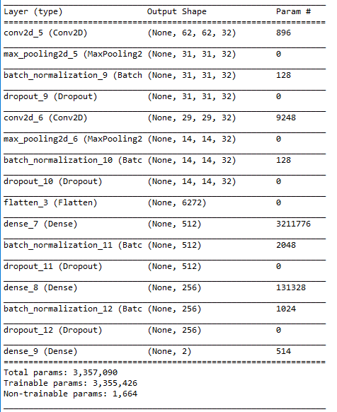
After hyperparameter search, our final architecture consists of two convolution layers. The input data is preprocessed and reduced its image size to $64\times 64$, which is fed into a convolution layer with 32 filters of $3\times 3$ size, with a stride of $1$. The result of convolution is $62\times 62\times 32$ feature array. Then the feature array is fed to a max-pooling layer of size $2\times 2$ and the resultant feature matrix becomes a $31x31x32$. Max pooling[14] reduces the computational resources required by reducing the size of the pixel of the feature matrix while keeping the feature intact. Regularisation[15] techniques called batch normalization is deployed across all $32$ parallel channels of the output of the max-pooling layer. The batch normalized feature matrix is added with a dropout layer, with a dropout factor equal to $0.2$. The convolution layer, max pooling layer, batch normalization layer, and drop-out[16] complete one layer convolution process in the architecture. The architecture is shown below.

Figure 2: The architecture of CNN

The output of one complete convolution layer is given to another convolution layer with 32 filters of $3\times 3$ size, with a stride of 1. The result of convolution is $29\times 29\times 32$ feature array. Then the feature array is fed to max-pooling layer of size $2\times 2$ and the resultant feature matrix becomes a $14\times 14\times 32$. Then, batch normalization is deployed across all $32$ parallel channels of the output of the max-pooling layer. The batch normalized feature matrix is added with a dropout layer, with a dropout factor equal to $0.2$.

After the two complete convolution layers, the feature size has reduced enough and most of the feature is extracted so that we can now connect it with the feed-forward network. The $14\times 14\times 32$ feature matrix is flattened which size becomes 6272. This flattened feature is fed to a feed-forward network of size 512, along with batch normalization and dropout. The feed-forward network is further added to another layer of 256 neurons with batch normalization and dropout. Finally, the output layer is connected with 2 neurons, and the activation function in the output layer is softmax. The activation of the rest of the layers is ’Rectified Linear unit(RELU)[17]’. The cost function for the error measurement is used as categorial_crossentropy, and the optimizer is ’adam’. The number of parameters to be learned are 3,357,090 (approx 3.5 million). With the available computation capacity, it took 20 minutes for training. A summary of the model is shown below.

Figure 3: Summary of Neural Network model

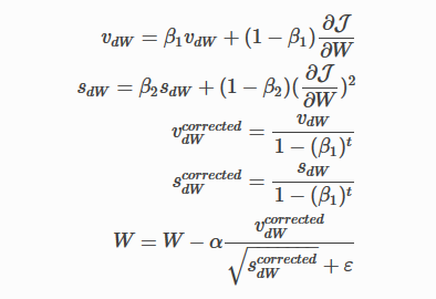
The optimizer that is used is called Adaptive Moment Estimation (Adam) [18], which combines ideas from both RMSProp and Momentum. It computes adaptive learning rates for each parameter.

Figure 4: Algorithm used during training

The loss function deployed is ’categorical_crossentropy’.Cross-entropy loss, or log loss, measures the performance of a classification model whose output is a probability value between 0 and 1. Cross-entropy loss increases as the predicted probability diverges from the actual label. So predicting a probability of .012 when the actual observation label is 1 would be bad and result in a high loss value. A perfect model would have a log loss of 0.

V Results

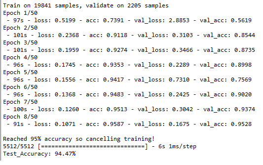
The model is trained and the result of the model and the cost function is shown below. The training and validation error is calculated simultaneously as the training progress. The number of epochs is set to 50, while a callback function is written to invoke early stopping when the model’s validation accuracy reaches 95% of accuracy. This is done to avoid overfitting (generalization error). If a callback is not deployed, the model over-fits and memorizes the training data. In such circumstances, the model gives 98% accuracy on training data but performs badly on validation and testing data. Once the training is done (which stops when validation accuracy reached 95%), then the testing error is calculated on the trained model. The testing accuracy achieved around 95.4%, which is satisfactory.

Figure 5: Result of training and testing

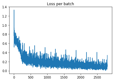
The plot of the cost function is calculated and it is plotted with respect to batch progression. The cost function initially drops sharply and then the rate is reduced. The batch gradient descent is used with a batch size of 64 images per batch. The result of batch training is the cost becomes noisy and fluctuates, but the overall trend of progression is toward optimal value. The cost function is plotted below.

Figure 6: Plot of cost with respect to batch

VI Related work

Machine learning is being used in control[19, 20, 21, 22, 23, 24] to model[25, 26] and prediction of complex systems [27, 28, 29, 30, 31, 32, 33].

There are various works in using machine learning in Malaria detection [34, 35] used deep CNN for Malaria detection but their model is more complex than ours. [34] used stacking-based approach for automated quantitative detection of Plasmodium falciparum malaria from blood smear. For the detection, a custom designed convolutional neural network (CNN) operating on focus stack of images is used. The cell counting problem is addressed as the segmentation problem and we propose a 2-level segmentation strategy. Use of CNN operating on focus stack for the detection of malaria improved the detection accuracy (both in terms of sensitivity [97.06%] and specificity [98.50%]) but also favored the processing on cell patches and avoided the need for hand-engineered features. [36] used machine learning for detection of Malaria. In 2016, Uganda’s Ministry of Health found that the disease is the leading cause of death in the country - accounting for 27 per cent of deaths. Mortality rates are particularly high in rural areas, where the lack of doctors and nurses is acute. Nursing assistants are often taught to read slides instead, but inadequate training can lead to misdiagnosis. Due to lack of availability of lab technicians in the region lead some to process four times as many as recommended number of screening in a day, while it is recommended that each technician should process no more than 25 slides each day. There are so many patients who may require malaria and TB tests, and overworking day and night. The AI lab([37], at Makerere University, has developed a way to diagnose the blood samples using a cell phone. The program learns to create its own criteria based on a set of images that have been presented to it previously. It learns to recognize the common features of the infections. The smartphone clamped in place over one microscope eyepiece brings to light a detailed image of the blood sample below - each malaria parasite circled in red by artificially intelligent software. With this AI backed technology, pathogens are counted and mapped out quickly, ready to be confirmed by a health worker. Diagnosis times could be slashed from 30 minutes to as little as two minutes. The AI software is built on deep learning algorithms that use an annotated library of microscope images to learn the common features of plasmodium parasites that cause malaria. Along with malaria paracites this lab also diagnosis the bacteria called Mycobacterium tuberculosis that is responsible for tuberculosis. Researchers at the Lister Hill National Center for Biomedical Communications (LHNCBC), part of National Library of Medicine (NLM), have developed a mobile application that runs on a standard Android smartphone attached to a conventional light microscope.

VII Conclusions

In this work , we showed a state of the art $2$ layer deep convolution network for Malaria diagnosis and detection. This method works with state of the art level accuracy without any expensive preprocessing.

References

- [1] H. Neema, H. Vardhan, C. Barreto, and X. Koutsoukos, “Web-based platform for evaluation of resilient and transactive smart-grids,” in 2019 7th Workshop on Modeling and Simulation of Cyber-Physical Energy Systems (MSCPES). IEEE, 2019, pp. 1–6.
- [2] C. Brosilow and B. Joseph, Techniques of model-based control. Prentice Hall Professional, 2002.
- [3] H. Vardhan, N. M. Sarkar, and H. Neema, “Modeling and optimization of a longitudinally-distributed global solar grid,” in 2019 8th International Conference on Power Systems (ICPS). IEEE, 2019, pp. 1–6.
- [4] A. Krizhevsky, I. Sutskever, and G. E. Hinton, “Imagenet classification with deep convolutional neural networks,” Communications of the ACM, vol. 60, no. 6, pp. 84–90, 2017.
- [5] H. Vardhan, U. Timalsina, P. Volgyesi, and J. Sztipanovits, “Data efficient surrogate modeling for engineering design: Ensemble-free batch mode deep active learning for regression,” arXiv preprint arXiv:2211.10360, 2022.
- [6] M. Bojarski, D. Del Testa, D. Dworakowski, B. Firner, B. Flepp, P. Goyal, L. D. Jackel, M. Monfort, U. Muller, J. Zhang et al., “End to end learning for self-driving cars,” arXiv preprint arXiv:1604.07316, 2016.
- [7] H. Vardhan and J. Sztipanovits, “Rare event failure test case generation in learning-enabled-controllers,” in 2021 6th International Conference on Machine Learning Technologies, 2021, pp. 34–40.
- [8] G. W. Gross, J. M. Boone, V. Greco-Hunt, and B. Greenberg, “Neural networks in radiologic diagnosis. ii. interpretation of neonatal chest radiographs.” Investigative Radiology, vol. 25, no. 9, pp. 1017–1023, 1990.
- [9] L. Sundaram, H. Gao, S. R. Padigepati, J. F. McRae, Y. Li, J. A. Kosmicki, N. Fritzilas, J. Hakenberg, A. Dutta, J. Shon et al., “Predicting the clinical impact of human mutation with deep neural networks,” Nature genetics, vol. 50, no. 8, pp. 1161–1170, 2018.
- [10] P. Ballester and R. M. Araujo, “On the performance of googlenet and alexnet applied to sketches,” in Thirtieth AAAI Conference on Artificial Intelligence, 2016.
- [11] “Nih data set.” [Online]. Available: https://ceb.nlm.nih.gov/repositories/malaria-datasets/
- [12] Y. LeCun et al., “Lenet-5, convolutional neural networks,” URL: http://yann. lecun. com/exdb/lenet, vol. 20, no. 5, p. 14, 2015.
- [13] H. Vardhan, P. Volgyesi, and J. Sztipanovits, “Fusion of ml with numerical simulation for optimized propeller design,” arXiv preprint arXiv:2302.14740, 2023.
- [14] N. Murray and F. Perronnin, “Generalized max pooling,” in Proceedings of the IEEE conference on computer vision and pattern recognition, 2014, pp. 2473–2480.
- [15] E. A. Smirnov, D. M. Timoshenko, and S. N. Andrianov, “Comparison of regularization methods for imagenet classification with deep convolutional neural networks,” Aasri Procedia, vol. 6, pp. 89–94, 2014.
- [16] P. Baldi and P. J. Sadowski, “Understanding dropout,” Advances in neural information processing systems, vol. 26, 2013.
- [17] A. F. Agarap, “Deep learning using rectified linear units (relu),” arXiv preprint arXiv:1803.08375, 2018.
- [18] D. P. Kingma and J. Ba, “Adam: A method for stochastic optimization,” arXiv preprint arXiv:1412.6980, 2014.
- [19] H. Vardhan and J. Sztipanovits, “Reduced robust random cut forest for out-of-distribution detection in machine learning models,” arXiv preprint arXiv:2206.09247, 2022.
- [20] Y. Duan, X. Chen, R. Houthooft, J. Schulman, and P. Abbeel, “Benchmarking deep reinforcement learning for continuous control,” in International conference on machine learning. PMLR, 2016, pp. 1329–1338.
- [21] S. Wang, W. Chaovalitwongse, and R. Babuska, “Machine learning algorithms in bipedal robot control,” IEEE Transactions on Systems, Man, and Cybernetics, Part C (Applications and Reviews), vol. 42, no. 5, pp. 728–743, 2012.
- [22] H. Vardhan and J. Sztipanovits, “Search for universal minimum drag resistance underwater vehicle hull using cfd,” arXiv preprint arXiv:2302.09441, 2023.
- [23] Z. Wu, A. Tran, D. Rincon, and P. D. Christofides, “Machine learning-based predictive control of nonlinear processes. part i: theory,” AIChE Journal, vol. 65, no. 11, p. e16729, 2019.
- [24] T. Duriez, S. L. Brunton, and B. R. Noack, Machine learning control-taming nonlinear dynamics and turbulence. Springer, 2017, vol. 116.
- [25] H. Neema, H. Vardhan, C. Barreto, and X. Koutsoukos, “Design and simulation platform for evaluation of grid distribution system and transactive energy,” in Proceedings of the 6th Annual Symposium on Hot Topics in the Science of Security, 2019, pp. 1–2.
- [26] C. Audet, J. Denni, D. Moore, A. Booker, and P. Frank, “A surrogate-model-based method for constrained optimization,” in 8th symposium on multidisciplinary analysis and optimization, 2000, p. 4891.
- [27] H. Vardhan, P. Volgyesi, and J. Sztipanovits, “Machine learning assisted propeller design,” in Proceedings of the ACM/IEEE 12th International Conference on Cyber-Physical Systems, 2021, pp. 227–228.
- [28] M. J. Volk, I. Lourentzou, S. Mishra, L. T. Vo, C. Zhai, and H. Zhao, “Biosystems design by machine learning,” ACS synthetic biology, vol. 9, no. 7, pp. 1514–1533, 2020.
- [29] H. Vardhan and J. Sztipanovits, “Deepal for regression using epsilon-weighted hybrid query strategy,” arXiv preprint arXiv:2206.13298, 2022.
- [30] S. Mazurenko, Z. Prokop, and J. Damborsky, “Machine learning in enzyme engineering,” ACS Catalysis, vol. 10, no. 2, pp. 1210–1223, 2019.
- [31] H. Vardhan, P. Volgyesi, and J. Sztipanovits, “Constrained bayesian optimization for automatic underwater vehicle hull design,” arXiv preprint arXiv:2302.14732, 2023.
- [32] S. M. Moosavi, K. M. Jablonka, and B. Smit, “The role of machine learning in the understanding and design of materials,” Journal of the American Chemical Society, vol. 142, no. 48, pp. 20 273–20 287, 2020.
- [33] H. Vardhan and J. Sztipanovits, “Deep learning based fea surrogate for sub-sea pressure vessel,” in 2022 6th International Conference on Computer, Software and Modeling (ICCSM). IEEE, 2022, pp. 36–39.
- [34] G. P. Gopakumar, M. Swetha, G. Sai Siva, and G. R. K. Sai Subrahmanyam, “Convolutional neural network-based malaria diagnosis from focus stack of blood smear images acquired using custom-built slide scanner,” Journal of biophotonics, vol. 11, no. 3, p. e201700003, 2018.
- [35] M. K. Gourisaria, S. Das, R. Sharma, S. S. Rautaray, and M. Pandey, “A deep learning model for malaria disease detection and analysis using deep convolutional neural networks,” International Journal of Emerging Technologies, vol. 11, no. 2, pp. 699–704, 2020.
- [36] M. Poostchi, K. Silamut, R. J. Maude, S. Jaeger, and G. Thoma, “Image analysis and machine learning for detecting malaria,” Translational Research, vol. 194, pp. 36–55, 2018.
- [37] “Uganda ai laboratory.” [Online]. Available: https://www.cnn.com/2018/12/14/health/ugandas-first-ai-lab-develops-malaria-detection-app-intl/index.html