Local Navigation Among Movable Obstacles
with Deep Reinforcement Learning

Abstract

Navigation in cluttered environments is still an open problem, especially when obstacles are movable. This is known as the Navigation Among Movable Obstacle (NAMO) problem. In this paper, we present a deep reinforcement learning approach for solving NAMO locally, near narrow passages. We train parallel agents in physics simulation using an Advantage Actor-Critic-based algorithm with a multi-modal neural network. We present an online policy that is able to push obstacles in a non-axial-aligned fashion, react to unexpected obstacle dynamics in real-time, and solve the local NAMO problem. Experimental validation in simulation shows that the presented approach generalizes to unseen NAMO problems in unknown environments. We further demonstrate the implementation of the policy on a real quadruped robot, showing that the policy can deal with real-world sensor noises and uncertainties in unseen NAMO tasks.

I INTRODUCTION

Studied extensively by Mike Stilman [1], the Navigation Among Movable Obstacle (NAMO) problem tackles planning problems where obstacles can be manipulated to aid a robot’s navigation in cluttered environments. Just like how humans intuitively nudge and move furniture out of their way when walking through a tightly packed room, robots could also benefit if they are able to plan obstacle pushes to clear path and reach their target location. Practical use-cases for NAMO solutions include robots that perform routine maintenance of factories, where idle containers and boxes may obstruct doorways; personal service robots in households, where rooms are packed with furniture and other items; and industrial inspection robots in underground caves and tunnels, where rocks and debris may block the walkway. In such environments, the ability to reliably push away obstacles will significantly increase the efficiency of autonomous navigation.

However, even simplified versions of the NAMO problem have been proven to be NP-hard [2, 3]. Past literature has tackled the NAMO problem using algorithms based on iterative and recursive methods [4, 5, 6], but usually with simplifications to the problem setting, such as prior knowledge of the environment, offline planning, and axial-aligned pushing. Only a few studies have tackled the online NAMO problem and considered the implications of sensor errors and unexpected object dynamics [7, 8]. Furthermore, methods utilizing recursive and iterative search-based techniques usually result in a computational complexity that is exponential to the number of local obstacles [5], and the search time in practice can sometimes be too long when many obstacles are present.

Figure 1: The environment observation is obtained via visual sensors and preprocessed into the desired state format. The input is fed into a trained policy network that computes a high-level action output for the robot to follow in the environment, in order to solve the local NAMO task.

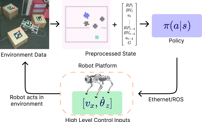
In this paper, we aim to address some of these shortcomings using a Deep Reinforcement Learning (DRL) approach (Fig. 1). By utilizing a neural network for policy-based RL algorithms, we develop an online agent that can solve unseen NAMO tasks without the constraint of axis-aligned pushing, and is able to handle uncertainties in sensor inputs and obstacle dynamics. Specifically, we focus on solving keyhole problems near one or two narrow passages. We also constrain the problem to use only pushing actions, as this is the most universal manipulation method amongst mobile robots and is still NP-Complete – pulling and lifting obstacles might also need extra robotic equipment such as arms and we leave it as future work. Our proposed method is suitable to be implemented within workflows where global path planning algorithms such as A* [9] would be unable to resolve local problems that require NAMO solutions. Therefore, we formulate the environment in a small region near narrow passages, with the objective of the robot reaching from one disjointed space to the other via obstacle pushing. Such framing of the problem removes the necessity for the RL agent to learn how to perform path planning with obstacle avoidance. The goal of the policy is only to get through the local narrow passage using obstacle pushing, such that reliable path tracking can resume.

We utilize a policy based on Advantage Actor-Critic algorithm [10], and we use the state-of-the-art physics engine NVIDIA Isaac Gym [11] to simulate and train parallel agents in obstructed narrow passages. We present results for both policies trained to solve unseen obstacle positions in known environments, and unseen obstacle positions in unknown environments. We further demonstrate real-world robot experiments conducted on a Unitree Go1 quadruped robot to show that the policy is able to handle sensor noises and real-world obstacle dynamics in practice.

The rest of this paper is organized as follows. In Sec. II, we discuss the literature on the NAMO problem, while in Sec. III we state the problem formulation in the reinforcement setting, and how we implement training in simulation. In Sec. IV we present our results both in simulation and with real robot experiments. Lastly, Sec. V concludes the paper and points to future directions for solving NAMO with RL.

II RELATED WORK

The complexity of motion planning with movable obstacles was first analyzed by [2], where simplified variations of NAMO have been proven to be NP-hard, while Demaine et al. [3] further showed that problems involving square blocks constrained to planar translations are still NP-hard. Stilman et al. [1] formulated NAMO as a graph-based planner that decomposes the global problem into a set of subclass keyhole problems called $LP_{1}$, where disjointed free spaces can be connected by moving a single obstacle. This work was extended in [4] for $k$ obstacles, namely the $LP_{k}$ sub-problem. In the same period, Nieuwenhuisen et al. [6] solved the problem probablistically using RRT and adaptive heuristics for the node expansion. Similarly, Berg et al. [12] decoupled the axis-aligned obstacle movements in a probabilistic algorithm. More recently, Moghaddam et al. [5] proposed a recursive algorithm capable of solving nonlinear and non-monotone problems with axis-aligned object manipulations, and a quadruped robot applied pushing actions to free space in [13] via search-based methods.

In the aforementioned approaches, planning is performed offline with complete prior knowledge of the environment and known movability of obstacles. The computational complexity of these methods grows exponentially to the number of obstacles, which is inefficient in practice as the number of obstacles in the scene increases. Wu et al. [14] studied NAMO in an unknown environment and object movability via pushing actions. An efficient online re-planning method was introduced when new information changes the optimality of the current plan. Kakiuchi et al. [7] devised an action strategy and performed real-world testing on humanoid robots for unknown environments and object movability. In Levihn et al. [15], a novel method was introduced based on Hierarchical RL and Monte Carlo Tree search, performing online planning with uncertain sensor information. The proposed method is shown to have approximately linear computational complexity with respect to the number of obstacles. Non-axial manipulation of obstacles is examined in [8] by utilizing a physics-based RL framework to adapt to unexpected obstacle behaviors such as rotation. Further extensions to NAMO, such as socially aware obstacle placement, have also been examined in [16, 17, 18].

In this paper, we utilize DRL which is proven to generalize to a wide range of tasks in simulation, such as navigation tasks [19], with agents performing highly difficult tasks with very little to no prior knowledge. Related to our work, Xia et al. [20] trained vision-based DRL agents in home settings with interactive objects, in a different context to NAMO; i.e., object manipulation to reach a goal, which is something we focus in our work. We highlight that our approach removes the constraint of axis-aligned pushing, and imposed positional (Pos.), movement (Mov.), and kinematics (Kin.) uncertainties in the environment. We further note that compared to [8], our method runs in constant time complexity and therefore completes a typical similar task about five times faster. Furthermore, our method is capable of solving harder problems such as non-linear problems, which we will demonstrate in Sec. III.

Figure 2: Our policy (multi-modal neural network). The state $s_{t}$ consists of a vector and a grid. The vector is $242$ long, with information about the agent’s pose, box vertices, previous action, and goal position. The grid consists of $48$ cells, semantically labeled. The vector is first passed through a linear block, whilst the grid image is passed forward via two convolution blocks and a linear block. The outputs of the two streams are concatenated, then passed through two more linear blocks. Finally, the network diverges via two separate sets of weights to output the value estimate and the action output.

The main contributions of this work are:

• We propose a DRL policy that can solve local NAMO problems with non-axial-aligned pushing, with constant computational complexity.

• We demonstrate that the proposed policy is able to work for unseen obstacle positions in known environments, and generalizes to unseen obstacle positions in unknown environments.

• We show that reliable sim-to-real transfer is possible to handle sensor noises and uncertain object dynamics.

III METHODS

III-A RL Background

We consider a typical episodic RL setting where the agent interacts with the environment over discrete timesteps. At every timestep, the agent receives state $s_{t}$ and samples an action ${a_{t}}$ from the policy distribution $\pi(a_{t}|s_{t};\boldsymbol{\theta})$, where $\boldsymbol{\theta}$ is the parameter of some function approximation. The agent then receives the next state $s_{t+1}$ and a scalar reward ${r_{t}}$. In policy-based settings, the objective is to find the parameter $\boldsymbol{\theta}$ which maximizes the expected cumulative return $R_{t}=\sum^{\infty}_{k=0}\gamma^{k}r_{t+k}$ with discount factor $\gamma\in(0,1]$.

In Advantage Actor-Critic methods, the algorithm computes both a policy $\pi(a_{t}|s_{t};\boldsymbol{\theta})$ and a value function $V(s_{t};\boldsymbol{w})$. The value function estimates the expected return $\mathbb{E}_{\pi}[R_{t}|s_{t}=s]$ by following the current policy $\pi$ from $s_{t}$. The value function $V$, also known as the critic, updates via the parameter $\boldsymbol{w}$ whilst the policy $\pi$, also known as the actor, updates via the parameter $\boldsymbol{\theta}$.

We implemented a deep neural network for function approximation and updated the parameters with stochastic gradient descent. The parameters are updated using

$$\boldsymbol{\theta}\leftarrow\boldsymbol{\theta}+\alpha\nabla_{\boldsymbol{\theta}}\log{\pi(a_{t}|s_{t};\boldsymbol{\theta}})A(s_{t},a_{t};\boldsymbol{w})$$ (1)

$$\boldsymbol{w}\leftarrow\boldsymbol{w}+\alpha_{w}\nabla_{w}V(s_{t};\boldsymbol{w})A(s_{t},a_{t};\boldsymbol{w})$$ (2)

where $\alpha$ and $\alpha_{w}$ represent the learning rate of the policy and value function, respectively. Note that $A(s_{t},a_{t};\boldsymbol{w})=\sum^{k-1}_{i=0}\gamma^{i}r_{t+i}+\gamma^{k}V(s_{t+k};\boldsymbol{w})-V(s_{t};\boldsymbol{w})$ computes the n-step advantage for the state-action pair ($s_{t}$, $a_{t}$), where $k$ determines the number of steps to look ahead.

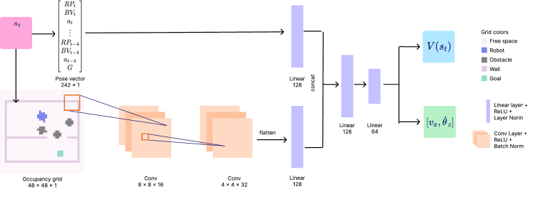
In practice, the actor and critic parameters $\boldsymbol{\theta}$ and $\boldsymbol{w}$ share a large set of weights, as shown in Fig. 2 to help stabilize the learning. In addition, we add an entropy term $\nabla_{\theta}H(\pi(s_{t};\boldsymbol{\theta}))$ to Eq. (1) and Eq. (2) as recommended by [10] to help regularize learning. We also use a clipped surrogate objective from [21]:

$$L^{CLIP}(\theta)=\hat{\mathbb{E}}_{t}\left[\text{min}(r_{t}(\theta)\hat{A}_{t},\text{clip}(r_{t}(\theta),1-\epsilon,1+\epsilon)\hat{A}_{t})\right]$$

where $\epsilon$ is a hyper-parameter to be set. Updating policies in such ways further improves the stability of training.

III-B Problem Formulation

We tackle local NAMO keyholes, with the objective being to connect two disjointed, adjacent free spaces separated by a set of obstacles. We define an agent which interacts with the environment over a set of timesteps, with continuous action space in forward velocity $v_{x}$ and angular velocity $\dot{\theta}_{z}$. The agent receives a reward $r_{t}$ from the environment at each timestep, and the objective is to maximize the cumulative return $\sum^{\infty}_{k=0}\gamma^{k}r_{t+k}$.

The environment consists of a small local region that includes a narrow passage obstructed by several obstacles. We set the goal behind the passage. The episode ends if the agent either reaches the goal or the maximum episode length is exceeded. We assume the following upstream inputs are present when constructing the state of the agent: a semantically labeled, coarse occupancy grid, which can be obtained via LiDAR or visual sensors and semantic segmentation methods [22]; obstacle bounding boxes, which can be obtained by object detection algorithms[23]; and internal pose data about the agent’s current state, which can be obtained via robot’s internal sensors. We assume a degree of sensor noise from all the inputs. From these upstream inputs, we then construct the agent state which includes the goal position $G$, obstacle vertices $BV_{t}$, robot internal state (pos, vel, rot, ang vel) $RP_{t}$, previous action $a_{t}$, and a semantically labeled occupancy grid. We include a history of concatenated past states for $RP_{t}$, $BV_{t}$, and $a_{t}$ to provide the agent with some temporal information, in a similar fashion as [24]. We choose to include the past $5$ frames, as from our experiments this was proved to provide a good trade-off between performance and computational cost. The final state is formed by the occupancy grid and a vector containing data $G$, $RP_{t-4:t}$, $BV_{t-4:t}$, and $a_{t-4:t}$, as shown in Fig. 2. In order to keep the policy practical and generalizable, we adopt a high-level control strategy to control the robots. We utilize a unicycle model with two degrees of freedom $v_{x}$ and $\dot{\theta}_{z}$, i.e., linear and angular velocity. This policy can easily be applied to different robot models, demonstrated in Sec. IV.

TABLE I: Reward given at each timestep

reward	description	weight
goal	1 if reach goal, 0 otherwise	10
progress	[-1, 1] $\propto$ velocity towards goal	1
dist	[0, 1] $\propto$ distance to goal	0.1
wall collision	-1 if collision with wall	0.2
box collision	-1 if collision with box	0.1
vel effort	$[-1,0]\propto v_{target}$ target velocity	0.05
rot effort	$[-1,0]\propto\dot{\theta}_{target}$	0.1
vel offset	$[-1,0]\propto|v_{actual}-v_{target}|$	0.2
rot offset	$[-1,0]\propto|\dot{\theta}_{actual}-\dot{\theta}_{target}|$	0.1
time	-1	1

The agent’s objective is to maximize the cumulative return. The reward given at each timestep is described in Table I. We give a large reward upon completion of the task, and no reward if the task is not completed. At each timestep, a small amount of positive reward is given if the agent moves towards the goal (progress), or is close to the goal (dist). A small amount of negative reward is also given proportionally to the effort of the action taken (vel effort, rot effort), any collision with walls (wall collision), and any contacts from pushing obstacles (box collision). We also penalize the agent for inducing large offsets between target and actual actions, which typically results from collisions with other objects or abrupt changes to actions (vel offset, rot offset).

III-C Algorithm Implementation

We train our agent in simulation using NVIDIA Isaac Gym [11] that can train parallel agents on a single GPU, towards stable and time efficient policy-based learning [10]. The advantage actor-critic method is implemented with a multi-modal neural network is designed to fuse two components of the state space, as illustrated in Fig. 2. The state includes a vector and grid component that are normalized to $[-1,1]$. The vector input is passed through a linear block consisting of one layer of perceptron with $128$ units, ReLU activation, and a normalization layer. The grid input is passed through two convolutional blocks each consisting of a convolutional filter, ReLU activation, and batch normalization. The first block contains $16$ filters of $8\times 8$, whilst the second block contains $32$ filters of $4\times 4$. The output is flattened and passed through a linear block with $128$ units. The two streams are concatenated and passes through two linear blocks with $128$ units and $64$ units. The output is then finally connected to two separate linear layers outputting the value estimate $V(s_{t})$ and the action $[v_{x},\dot{\theta}_{z}]$, respectively.

Figure 3: Fixed maps and random obstacle positions. Agents (gray) need to push boxes (yellow) to reach the goal (green). The maps include corridors (a,b), mid (c,d), side (e,f), and diagonal (g,h) doorways.

III-D Scene Generation and Curriculum Training

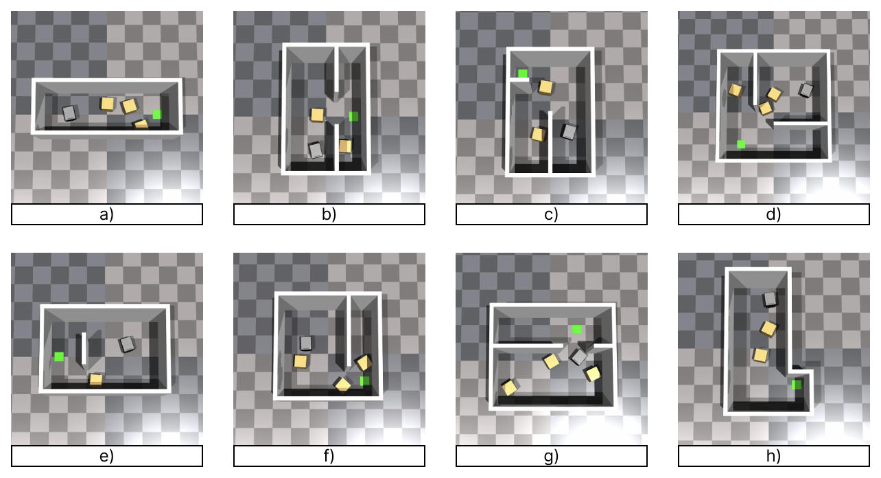
In Fig. 3, we show eight different map configurations that were developed in Isaac Gym. We designed these maps to cover a wide range of local NAMO settings: narrow corridor (map $a$ and $b$), doorway with space to the sides (map $c$ and $d$), doorway against a wall (map $e$, $f$ and $i$), and diagonal doorways (map $g$ and $h$).

Each agent is spawned in a predefined room with a dimension around $6\times 6$ $m^{2}$. This is a reasonable setting for mobile robot sizes of around $0.5$ to $1$ meter in length to move through narrow passages that are $1$ to $2$ meters wide. An obstruction of obstacles near such passages would make it difficult for the robot to pass through. The robot and the goal position are randomly spawned within their own predefined area, but with a small probability (e.g., $5\%$) the robot can also spawn anywhere inside the map, such that the agent has a finite chance of visiting every position.

Figure 4: The reward over policy update steps for single and multiple maps are shown in purple and green, respectively. Curriculum learning can be observed from sharp drops of the purple curve as the task becomes harder; in multiple maps it is smoothed out as not all reach curriculum simultaneously. The single map setting converges to a stable equilibrium, compared to the multiple one that early stopping is performed.

We choose boxes of size around $60cm^{3}$, and spawn up to $5$ boxes in each room. We choose $5$ boxes because it appropriately fills the room with enough variety, adding more would overfill the room and make the box position generation too difficult. Note that if obstacle positions are generated at random, most of the problems would be too easy, i.e., not requiring any interaction between the agent and the obstacles. Therefore, obstacle positions are picked randomly with a higher probability to spawn in difficult positions. Concretely, each obstacle $i$ has probability $\lambda p_{i}$ to spawn in any random location in the room, with random rotation. With probability $\lambda(1-p_{i})$ it spawns in predefined challenging positions (e.g. that blockades the narrow passage, or positioned near the narrow passage) plus some random perturbations. Finally, with probability $1-\lambda$ the obstacle does not spawn in the room, in which case their vertices are represented with zeros in the input. We typically use $p_{i}\in[0.2,0.6]$ for each box, and we gradually increase the value of $\lambda$ in discrete increments starting from $0.2$. By randomizing the positions of obstacles, we force the agent to find a solution for new obstacle positions every time, and thereby learn to reason about the relationship between different obstacles, such as which order to push the obstacles.

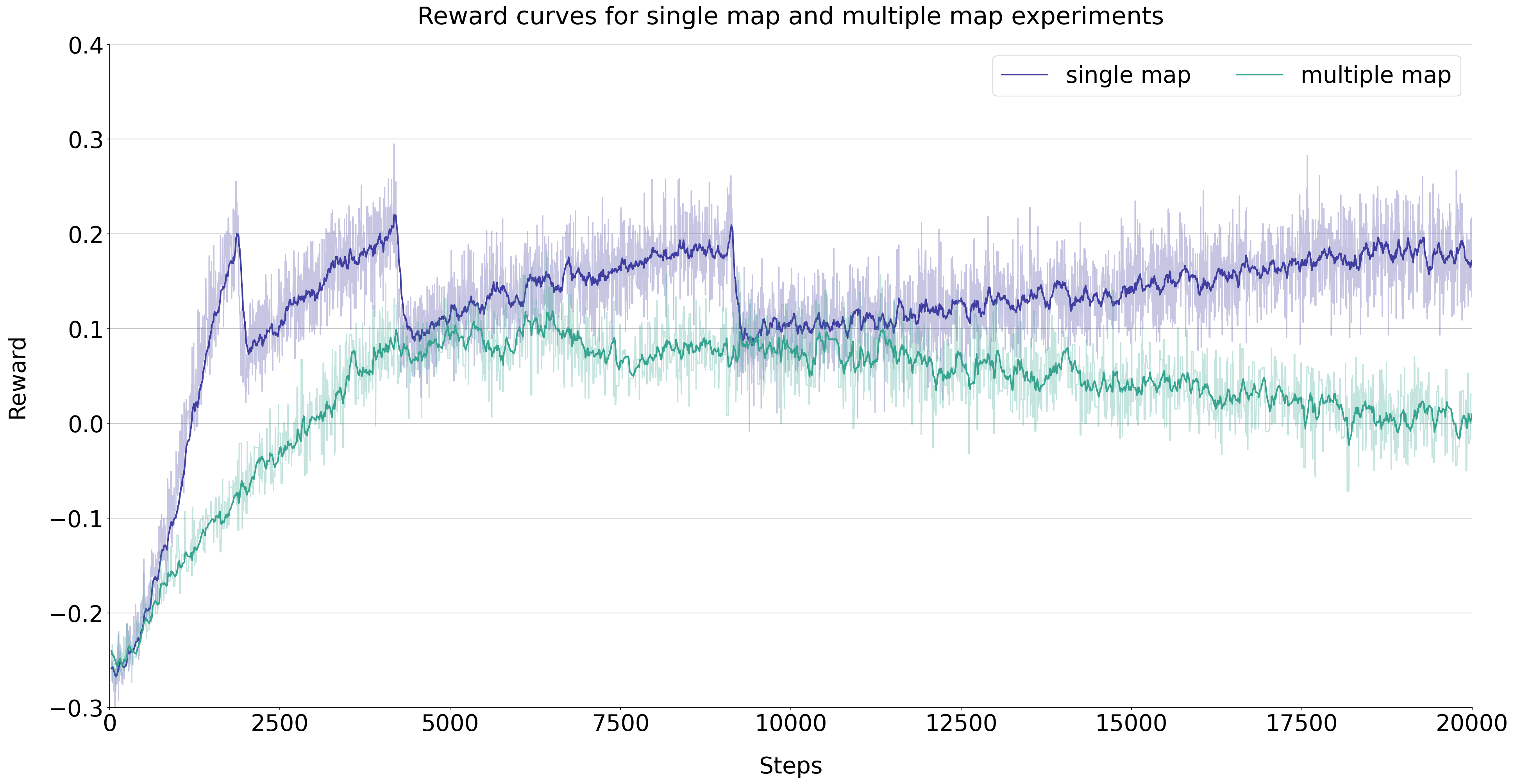
The parameter $\lambda$ allows us to control how many boxes spawn and thereby the difficulty of the NAMO problem. This effectively creates a curriculum training scheme where we can update $\lambda$ such that the agent receives more difficult problems as it learns to solve easier ones. We set a threshold of completion rate at the current difficulty (e.g., $90\%$). Starting with $\lambda=0.2$, we train the agent until its performance reaches $90\%$ completion rate, and we increase $\lambda$ by $0.2$. This process repeats $4$ times until $\lambda$ reaches $1$, upon which around $4$ to $5$ boxes will spawn at the start of the scene every time. The effect of this curriculum learning scheme over a training run can be seen in Fig. 4.

III-E Domain Randomization

Heavy domain randomization is applied to both the state and the action space in the form of Gaussian white noise. We anticipate real-world problems to be highly noisy in both sensor inputs and object dynamics, and a good policy should be able to robustly handle such noises. By adding noises to input state space, we simulate sensor noises that the robot is likely to encounter in the real world, such as temporal fluctuations in estimated obstacle poses and robot pose. Note that we add noises to the vector state and the grid state independently, as the real-world sources of these sensor noises are usually not correlated. We add similar Gaussian noise to the action outputs of the model, in order to simulate unexpected robot dynamics. Overall, applying domain randomization in our training decreases the sim-to-real gap, and ensures that the policy is stable in the presence of noisy inputs and unexpected object dynamics, as we will demonstrate in the next section.

IV EXPERIMENTS

Figure 5: Qualitative simulated results on single map setting: the agent adapts to different obstacle positions and finds efficient paths.

IV-A Simulation

Firstly, test the trained policy both quantitatively and qualitatively in simulation. We train with two settings: single and multiple rooms. In the single room, we train the agent with random box positions (Fig. 5, whilst in the multiple rooms we have eight different room layouts. Our results show that in the single room configuration, we can train a policy to generalize to unseen obstacle positions in a known environment with optimized behaviors and a low failure rate. In the multiple room setting, a policy can also generalize to unseen obstacle positions in unseen environments at the cost of a less optimized behavior.

The following training settings are used for both experiments. The scene generation and randomization protocols are described in Sec. III, where we randomize the positions of the agent, goal, and boxes, train with a curriculum, and apply domain randomization to the input and output space. We use ADAM as the optimizer [25], with l2 regularization to help with stability [26]. We also add gradient clipping to avoid exploding gradients, which typically occurs when off-policy learning, function approximation, and value bootstrapping are all present (deadly triad) [27]. An adaptive learning rate is utilized based on the KL threshold. We use a horizon length of $50$, and policy update frequency of $20$ physics steps ($333$ms). The maximum episode length is set to $45$ seconds, or $2700$ physics steps. We train $4,000$ environments in parallel with mini-batch of $2,000$ samples every update. Training is conducted using an NVIDIA RTX 3080 GPU for $20,000$ policy update steps.

Figure 6: Qualitative simulated results on multiple map setting: a) the agent pushes obstacles sequentially, whilst making minimal detours to its trajectory; b) the agent recovers from unexpected dynamics.

TABLE II: Performance of policy when trained on single map configuration with varying $\lambda$

$\lambda$	boxes	completion rate	time taken	boxes pushed
0	0	99.9	6.80	0
0.2	0.7	98.5	7.13	0.34
0.4	1.3	98.3	7.68	0.64
0.6	2.1	97.4	8.09	1.00
0.8	2.8	94.5	8.14	1.37
1	3.7	91.0	8.69	1.92

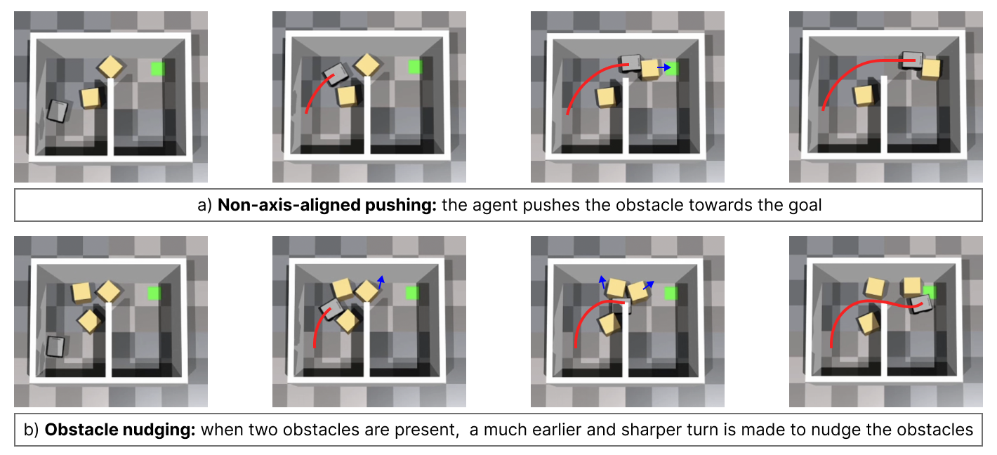
In the first experiment with a single map setting, we train the policy on the same map (see Fig. 5) but randomize the initial agent, goal, and obstacle positions. We then evaluate the network with $1,000$ scenes in the same map configuration but with unseen box positions. We repeat the evaluation six times by varying the parameter $\lambda$ to increase the number of boxes in the scene, thereby increasing the difficulty of the problems. Fig. 5 illustrates some qualitative results of the experiment. In the top row, we see that the agent is able to push obstacles along a trajectory in a non-axis-aligned fashion along its trajectory. In the second row, we highlight that the agent takes a much more narrow turn at the doorway because the most efficient way to get through is by nudging both boxes aside. This is because pushing boxes into the door will cause them to block the goal (shown in green). We highlight that the demonstrated behaviors cannot be achieved with the restriction of axis-aligned pushing, which many past works require.

Figure 7: From left to right: [t=0] Green dot is the goal. The robot: [t=4] avoids collision with box 3; [t=8] moves box 2 to create small opening; [t=10] stops pushing box 2 and rotates towards box 1; [t=12] pushes box 1 out of the door. [t=23] Goal reached. The robot performs non-axis-aligned pushing.

The quantitative results of this experiment are shown in Table II. The rows represent increased difficulty from top to bottom as $\lambda$ increases. Note that the number of boxes in the scene is not directly proportional to $\lambda$ due to the random box spawning, as sometimes there are no more vacancies left for new boxes to spawn. We observe that as the problem becomes harder with more boxes, the completion rate decreases often due to the agent being stuck in an unrecoverable position such as a blocked pathway or blocked goal position. In the last column of the table we list the number of mean boxes pushed when the task is completed. We note that this value is usually only half of the mean number of boxes in the scene, demonstrating that the agent only pushes boxes that are necessary for clearing the path. Overall, the observed agent’s behavior is stable and robust in the single map setting. It is able to generalize to unseen obstacle positions to find the correct solution in unseen initial configurations $91\%$ of the time, even in the hardest tasks.

TABLE III: Comparison between policy performance on training maps and test map, with $\lambda=0.8$

Experiment	completion rate	time taken (s)	boxes pushed
Training (8 maps)	79.8	10.99	1.12
Testing (unseen map)	54.3	13.05	1.51

In the second experiment, we train one policy on multiple maps simultaneously and examine whether or not the trained policy is able to generalize to unseen environments as well as unseen obstacle positions. We train the agent on maps $a$ to $h$, shown in Fig. 3, and test the agent on $1,000$ environments with an unseen map (same map shown used in single map setting). Our results show that the stability of learning is difficult to maintain in this setting. Despite having utilized several regularization techniques, stable convergence of the policy is still not guaranteed on every run. Fig 4 shows that the policy is unable to reach the same performance as the single map case. Therefore, we perform early stopping to pick a policy snapshot that performs best during training.

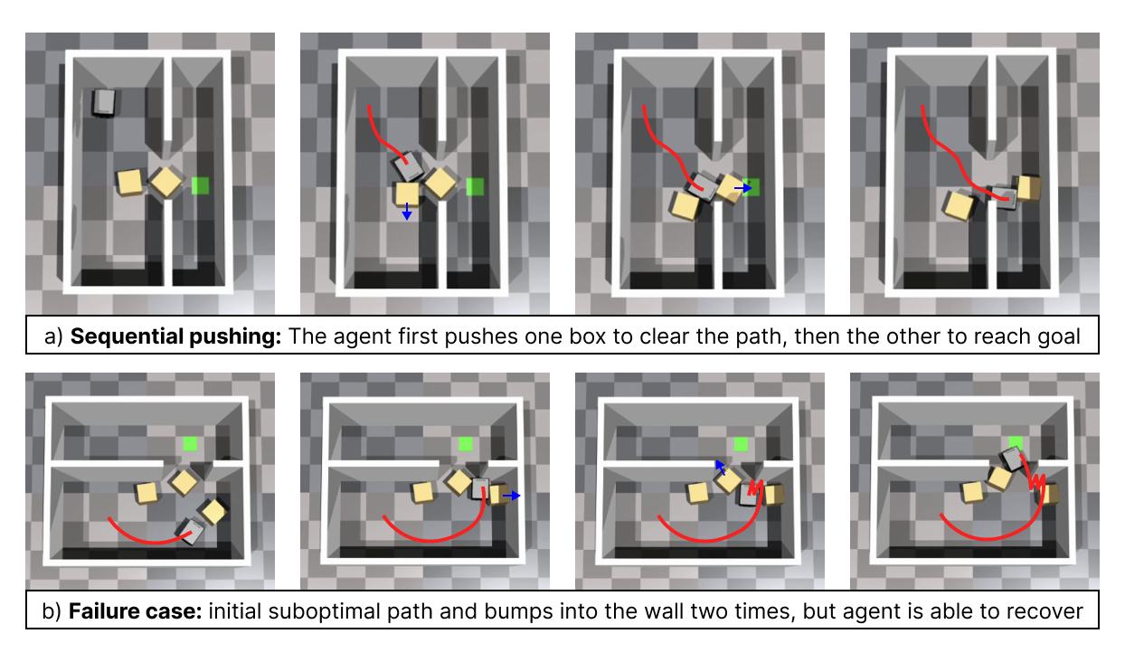
In the multiple map settings, the agent learns strategies that generalize across different tasks, i.e., sequentially pushing obstacles and reacting in real-time to unexpected dynamics and input noises. Fig. 6-a shows an example of non-linear sequential pushing (pushing the left before the right box). We highlight that the agent is able to optimize this behavior by making only small detours along its trajectory, which would not usually be possible to achieve with axis-aligned pushing constraints. Fig 6-b highlights the ability of the agent to recover from an undesirable position. Due to limited resolution in the input image, it’s often hard for the agent to precisely localize the doorway and it sometimes runs into the wall near the doorway, as shown in frame $2$. However, when such expected dynamics occur in the environment, the agent adopts a strategy of backing out and moving forward again to get through the passage, shown in frames $3$ and $4$. Such behavior illustrates that a less optimal policy is reached compared to the single map setting, however, the agent still displays interesting ways to recover itself from a bad state.

The quantitative results are shown in Table III. We test the performance of the agent in known environments (same eight maps) but unknown obstacle positions and environment. The agent achieves around $80\%$ completion rate across all eight maps in the hardest cases and achieves $54\%$ completion rate in an unseen map. Whilst the completion rate on the unseen environment is relatively lower, it still demonstrates such an ability. The performance could possibly be increased further with higher training data randomization and by repeating experiences on harder NAMO problems via prioritized experience replay [28].

IV-B Failure Cases

In the single map setting, most failures often involve the agent pushing the box into an unrecoverable position, such that the passage is completely blocked. On the other hand, in the multiple map setting, we see more failures. This often includes agents taking unnecessary turns and sometimes getting stuck in a corner, as seen in Fig. 6. We believe this is caused by a combination of insufficient feature extraction from a neural network trained on highly correlated data, and a lack of resolution in the input image. The former can be improved by increasing the number of training maps and using experience replay to decorrelate the data, and the latter can be improved by increasing the input image dimension.

IV-C Robot Experiments

In this section, we present our results with a real quadruped robot (Unitree Go1), enhanced with aluminum struts that help in pushing obstacles. We use cardboard boxes as obstacles, with size of around $50\times 50\times 50cm^{2}$. The friction between boxes and the carpet does not allow the robot to push more than one box at once. We use two bird’s eye view cameras to track the obstacles (vertices) and robot (pose) using ArUco Markers [29]. Using those we compute a 2D grid to construct the state space. The implementation of obstacle detection and mapping is outside the scope of this paper, and we only show that the robot is able to handle sensor noises and unexpected obstacle behaviors. We use a neural network trained in the single map setting, as it produces more robust and stable results, and shows that the presented policy can be implemented in real-world, where uncertain robot dynamics and sensor inputs are present.

Our testing shows that the robot can consistently navigate through narrow passages with obstacles (Fig. 7). The robot needs to reach the green dot, and solves the NAMO problem by avoiding collision with box $3$ (at $t=4$), move box $2$ via rotational pushing just enough for an opening to occur (at $t=10$), and pushing box $1$ out of the doorway until it reaches the goal (at $t=23$). We observed that it’s very typical for the robot to perform pushing follow non-linear trajectories, with only small nudges to rotate the obstacle, which is often the most efficient way to create small openings.

V CONCLUSIONS AND FUTURE WORKS

In this paper, we presented a DRL method that allows a robot to perform non-axial pushing to solve $LP_{k}$ NAMO problems with constant computational complexity. We demonstrated the method in simulation and on a real robot with sensor noises. In the future, we aim at stabilizing learning for agents trained in multiple maps. We aim at also investigate how agents can deal with obstacles with unknown movability and unseen shapes by incorporating these complexities in the training.

References

- [1] M. Stilman and J. J. Kuffner, “Navigation Among Movable Obstacles: Real-Time Reasoning in Complex Environments,” World Scientific IJHR, vol. 2, no. 04, pp. 479–503, 2005.
- [2] G. Wilfong, “Motion Planning in the Presence of Movable Obstacles,” in 4th Annual Symp. on Computational Geometry, 1988, pp. 279–288.
- [3] E. D. Demaine, M. L. Demaine, and J. O’Rourke, “Pushpush and push-1 are np-hard in 2d,” 12th Canadian Conference on Computational Geometry, pp. 211–219, 2000.
- [4] M. Stilman and J. Kuffner, “Planning Among Movable Obstacles with Artificial Constraints,” The International Journal of Robotics Research, vol. 27, no. 11-12, pp. 1295–1307, 2008.
- [5] S. K. Moghaddam and E. Masehian, “Planning robot navigation among movable obstacles (namo) through a recursive approach,” Journal of Intelligent & Robotic Systems, vol. 83, pp. 603–634, 2016.
- [6] D. Nieuwenhuisen, A. Stappen, and M. H. Overmars, “An Effective Framework for Path Planning Amidst Movable Obstacles,” in Springer Algorithmic Foundation of Robotics VII, 2008, pp. 87–102.
- [7] Y. Kakiuchi, R. Ueda, K. Kobayashi, K. Okada, and M. Inaba, “Working with Movable Obstacles using On-line Environment Perception Reconstruction using Active Sensing and Color Range Sensor,” in IEEE/RSJ IROS, 2010, pp. 1696–1701.
- [8] J. Scholz, N. Jindal, M. Levihn, C. L. Isbell, and H. I. Christensen, “Navigation Among Movable Obstacles with Learned Dynamic Constraints,” in IEEE/RSJ IROS, 2016, pp. 3706–3713.
- [9] P. E. Hart, N. J. Nilsson, and B. Raphael, “A Formal Basis for the Heuristic Determination of Minimum Cost Paths,” IEEE Transactions on Systems Science and Cybernetics, vol. 4, no. 2, pp. 100–107, 1968.
- [10] V. Mnih, A. P. Badia, M. Mirza, A. Graves, T. Lillicrap, T. Harley, D. Silver, and K. Kavukcuoglu, “Asynchronous Methods for Deep Reinforcement Learning,” in PMLR International Conference on Machine Learning, 2016, pp. 1928–1937.
- [11] V. Makoviychuk et al., “Isaac Gym: High Performance GPU-Based Physics Simulation for Robot Learning,” arXiv preprint arXiv:2108.10470, 2021.
- [12] J. v. d. Berg, M. Stilman, J. Kuffner, M. Lin, and D. Manocha, “Path Planning Among Movable Obstacles: a Probabilistically Complete Approach,” in Springer Algorithmic Foundation of Robotics VIII, 2009, pp. 599–614.
- [13] V. S. Raghavan, D. Kanoulas, D. G. Caldwell, and N. G. Tsagarakis, “Reconfigurable and Agile Legged-Wheeled Robot Navigation in Cluttered Environments With Movable Obstacles,” IEEE Access, vol. 10, pp. 2429–2445, 2022.
- [14] H. N. Wu, M. Levihn, and M. Stilman, “Navigation Among Movable Obstacles in Unknown Environments,” in IEEE/RSJ International Conference on Intelligent Robots and Systems, 2010, pp. 1433–1438.
- [15] M. Levihn, J. Scholz, and M. Stilman, “Hierarchical Decision Theoretic Planning for Navigation Among Movable Obstacles,” in Springer Algorithmic Foundations of Robotics X, 2013, pp. 19–35.
- [16] B. Renault, J. Saraydaryan, and O. Simonin, “Towards S-NAMO: Socially-aware Navigation Among Movable Obstacles,” in Springer Robot World Cup, 2019, pp. 241–254.
- [17] K. Ellis, H. Zhang, D. Stoyanov, and D. Kanoulas, “Navigation Among Movable Obstacles with Object Localization using Photorealistic Simulation,” in IEEE/RSJ IROS, 2022.
- [18] K. Ellis et al., “Navigation Among Movable Obstacles via Multi-Object Pushing Into Storage Zones,” IEEE Access, vol. 11, pp. 3174–3183, 2023.
- [19] P. Mirowski, R. Pascanu, F. Viola, H. Soyer, A. J. Ballard, A. Banino, M. Denil, R. Goroshin, L. Sifre, K. Kavukcuoglu et al., “Learning to Navigate in Complex Environments,” arXiv preprint arXiv:1611.03673, 2016.
- [20] F. Xia, W. B. Shen, C. Li, P. Kasimbeg, M. E. Tchapmi, A. Toshev, R. Martín-Martín, and S. Savarese, “Interactive Gibson Benchmark: A Benchmark for Interactive Navigation in Cluttered Environments,” IEEE RA-L, vol. 5, no. 2, pp. 713–720, 2020.
- [21] J. Schulman, F. Wolski, P. Dhariwal, A. Radford, and O. Klimov, “Proximal Policy Optimization Algorithms,” arXiv preprint arXiv:1707.06347, 2017.
- [22] A. Rosinol, M. Abate, Y. Chang, and L. Carlone, “Kimera: an Open-Source Library for Real-Time Metric-Semantic Localization and Mapping,” in IEEE ICRA, 2020, pp. 1689–1696.
- [23] B. Wen, J. Tremblay, V. Blukis, S. Tyree, T. Müller, A. Evans, D. Fox, J. Kautz, and S. Birchfield, “BundleSDF: Neural 6-DoF tracking and 3D reconstruction of unknown objects,” in CVPR, 2023.
- [24] V. Mnih et al., “Human-level Control through Deep Reinforcement Learning,” Nature, vol. 518, no. 7540, pp. 529–533, 2015.
- [25] D. P. Kingma and J. Ba, “Adam: A Method for Stochastic Optimization,” in 3rd ICLR, 2014.
- [26] J. Farebrother, M. C. Machado, and M. Bowling, “Generalization and Regularization in DQN,” arXiv preprint arXiv:1810.00123, 2018.
- [27] R. S. Sutton and A. G. Barto, Reinforcement Learning: An Introduction. MIT press, 2018.
- [28] T. Schaul, J. Quan, I. Antonoglou, and D. Silver, “Prioritized experience replay,” arXiv preprint arXiv:1511.05952, 2015.
- [29] S. Garrido-Jurado, R. Muñoz-Salinas, F. J. Madrid-Cuevas, and M. J. Marín-Jiménez, “Automatic Generation and Detection of Highly Reliable Fiducial Markers Under Occlusion,” Elsevier Pattern Recognition, vol. 47, no. 6, pp. 2280–2292, 2014.