Structural dynamics of a model of amorphous silicon

Abstract

We perform extensive simulations and systematic statistical analyses on the structural dynamics of a model of amorphous silicon. The simulations follow the dynamics introduced by Wooten, Winer and Weaire: the energy is obtained with the Keating potential, and the dynamics consists of bond transpositions proposed at random locations and accepted with the Metropolis acceptance ratio. The structural quantities we track are the variations in time of the lateral lengths ($L_{x}$, $L_{y}$, $L_{z}$) of the cuboid simulation cell. We transform these quantities into the volume $V$ and two aspect ratios $B_{1}$ and $B_{2}$. Our analysis reveals that at short times, the mean squared displacement (MSD) for all of them exhibits normal diffusion. At longer times, they cross over to anomalous diffusion, with a temperature-dependent anomalous exponent $\alpha<1$. We analyze our findings in the light of two standard models in statistical physics that feature anomalous dynamics, viz., continuous time random walker (CTRW) and fractional Brownian motion (fBm). We obtain the distribution of waiting times, and find that the data are consistent with a stretched-exponential decay. We also show that the three quantities, $V$, $B_{1}$ and $B_{2}$ exhibit negative velocity autocorrelation functions. These observations together suggest that the dynamics of the material belong to the fBm class.

[inst1]organization=Department of Information and Computing Sciences, Utrecht University,addressline= Princetonplein 5 , city=Utrecht, postcode=3584 CC, country=The Netherlands

1 Introduction

Amorphous silicon (a-Si) has attracted a lot of attention in the computational materials science community over the last decades, partly because it is a material with many applications, and partly because it has become a prototypical example of a covalently bonded disordered material that lends itself well for simulations, as many empirical and semi-empirical potentials are readily available. There exist a myriad of experimental and simulation research works on the properties of a-Si, studying thermal transport [1, 2], structure and defects recognition [3], electronic properties and applications for solar cells [4, 5, 6], and vibrational properties [7]. Compared to structural and electronic properties, the dynamics of a-Si is less studied. In this paper we fill the knowledge gap on how structural properties of the material evolve in time. Dynamics of covalently-bonded materials are well-known to be extremely slow. On the one hand, it makes them highly stable, but on the other it renders them nearly impossible to be accessed by experimental time scales. Computer simulations can provide a way forward, but there too, simulation studies of a-Si dynamics have often focused on how to generate well-relaxed samples as efficiently as possible, but do not study the fundamental properties of its dynamics.

In this paper, we employ a relatively simple model for the dynamics of a-Si, as first introduced by Wooten, Winer and Weaire (WWW) [8]. The atomic structure in this model is described as a so-called continuous random network (CRN), in which each silicon atom has exactly four covalent bonds to other silicon neighbors. To each CRN-configuration, an energy is attributed using the Keating potential [9]. The dynamics consists of a sequence of bond transpositions proposed at random locations, and accepted or rejected according to the Metropolis algorithm. This technique allows for the simulation of the dynamics of a-Si over time scales that are much longer than those accessible to molecular dynamics (MD), at the expense of being a much cruder description. There is a however a connection between the two time scales. Within our Monte Carlo (MC) dynamics, the probability that a specific bond transposition is proposed in one MC unit of time is $2/(4*3*3*N)=1/(18N)$. Here, factors $1/N$, $1/4$, $1/3$ and $1/3$ respectively arise from picking a random atom (out of $N$ total atoms), then one of its four neighbours, next twice one of the three remaining neighbors, and the factor of $2$ comes from the possibility to generate the same string of atoms from two different ends. The acceptance probability is then $\exp(-\beta\Delta E)$, where $\Delta E$ is the energy difference between the initial and final states. Thus, the rate of structural changes in the sample is $(1/18N)\exp(-\beta\Delta E)$.

In molecular dynamics (MD), the rate would be $\nu\exp(-\beta B)$ where $\nu$ is the attempt frequency, often found to be around $10^{-12}$ s^-1=1 ps^-1, and $B$ is the energy barrier between the initial and final states. The energy barrier $B$ and the energy change $\Delta E$ are correlated, but loosely. For instance, we know that $B$ has to be higher than $\Delta E$. For example, from earlier work [Ref. [10], Table 1] we know that on average for bond transpositions (WWW events), $\langle\Delta E\rangle=4.0$ eV and $\langle B\rangle=2.2$ eV. As a rough estimate of $\Delta E-B$, we can then take $\langle B\rangle-\langle\Delta E\rangle=1.8$ eV. Our simulations were carried out at a temperature of 0.14 eV, with $N=2000$ atoms. We then obtain that one unit of MC time corresponds roughly to $(1/(18N))\exp(1.8/0.14)$ ps $\approx$ 10 ps.

In our simulations, we use a cuboid simulation cell with periodic boundary conditions, and lateral dimensions $L_{x}\times L_{y}\times L_{z}$. At all times, these lateral dimensions, together with all the atoms, constitute $N+3$ degrees of freedom. After each WWW move, the bond list is updated, and all degrees of freedom are minimized to the global minimum of energy, and consequently these lateral dimensions of the simulation cell will fluctuate in time. In our case, these fluctuations are easily accessible in simulations, and are closely related to the mechanical deformations under (small) external forces, and therefore a standard approach for understanding the mechanical shear and stress properties of the bulk material. All dynamics studied in the paper is performed at the temperature below the melting temperature of a-Si (1750K[11]).

We transform the three quantities $L_{x}(t)$, $L_{y}(t)$ and $L_{z}(t)$ into three other quantities, which are the volume $V(t)\equiv L_{x}(t)\cdot L_{y}(t)\cdot L_{z}(t)$ and the two aspect ratios $B_{1}(t)=L_{y}(t)/L_{z}(t)$ and $B_{2}(t)=L_{y}(t)\cdot L_{z}(t)/L_{x}^{2}(t)$. The aspect ratios $B_{1}(t)$ and $B_{2}(t)$ are two (almost) unconstrained degrees of freedom, which can vary over a wide range of values without preference. This however does not hold for the volume $V(t)$ as it is constrained to fluctuate around an ideal value set by the number of atoms and the ideal density. (It is well-known that well-relaxed samples of a-Si can be obtained within a wide range of densities: fluctuations of several percent are easily observed. Thus, the constraint is rather loose for this specific material.)

The focus of this paper lies on the dynamics of $V$, $B_{1}$ and $B_{2}$. The motivation for this choice is that these are quantities that lend themselves well for computer simulations studies, and are directly connected to the mechanical behavior under shear, stress, etc., which are of experimental relevance. Our findings indicate that over short time scales, all three quantities exhibit diffusive behavior; this is to be expected, as over a short time, the dynamics consist of local atomic rearrangements which cause random changes in $B_{1}$, $B_{2}$ and $V$ which are uncorrelated. At longer times, a negative velocity autocorrelation emerges: a positive change induces a bias at later times to be followed by a negative change, vice versa. These correlations are strong enough to change the dynamics from ordinary to anomalous diffusion: the mean squared deviations MSD₁, MSD₂ and MSD_V for $B_{1}$, $B_{2}$ and $V$ can be fitted by a power-law $\sim t^{\alpha}$ with $\alpha<1$. The exponent is found to be temperature-dependent. (Given that $V(t)$ is constrained to fluctuate around an ideal value as noted above would mean that the mean-square displacement of $V$ must reach a plateau at a long time. Our simulation times are however not long enough, i.e., the mean-square displacement of $V$ does not reach a high enough value to be influenced by the constraint.)

We analyze our findings in the light of standard models for anomalous diffusion, viz., the continuous time random walk (CTRW) model and fractional Brownian motion (fBm). For this purpose, we also determine numerically the distribution of the waiting times. This distribution can be well fitted by a function with stretched-exponential decay. Although this is different from homogeneous, memoryless materials, where the decay is expected to be exponential, the decay is still too steep to be the sole explanation of anomalous diffusion. We also determine the velocity autocorrelation functions, and find them to be negative at all times.

The organization of this paper is as follows. In Sec. 2, we introduce the model and simulation methods in detail. In Sec. 3.1, we define the structural quantities related to the mechanical properties, analyze the trajectories extracted from simulations, investigate the short-time behavior of mean-square displacements, and describe the relationships among the different diffusion coefficients. In Sec. 3.2, we analyze the probability distribution, both on waiting time and jump length, characterize sub-diffusive behaviors at long times, and reflect on the classification of the model. In Sec. 4 we summarize and conclude the paper.

2 The model

Figure 1: (color online) An initial sample of amorphous silicon with 2000 atoms, each connected to four neighboring atoms. The bonds have comparable length (2.35Å with a spread of 0.085Å), and the bond angles are close to the tetrahedral angle ($109.46^{\circ}$ with a spread of $9.5^{\circ}$). The sample has been generated, starting from a Voronoi diagram and then evolved using the WWW-algorithm, as discussed in Sec. 2. It is a cuboid with periodic boundaries on the lateral dimensions $L_{x}$, $L_{y}$ and $L_{z}$.

The Keating potential is one of the simplest and most efficient models for describing a-Si. It uses an explicit list of bonds: whether two atoms interact with each other or not, is thus determined by this bond list, and not by the distance between the atoms. It is defined as

$$E = \frac{3}{{16}}\frac{\alpha}{{{d^{2}}}}\sum\limits_{<ij>}{({\textbf{r}_{ij}}\cdot{\textbf{r}_{ij}}}-{d^{2}}{)^{2}}+\frac{3}{8}\frac{\beta}{{{d^{2}}}}\sum\limits_{<ijk>}{({\textbf{r}_{ij}}\cdot{\textbf{r}_{ik}}+\frac{1}{3}}{d^{2}}{)^{2}}.$$ (1)

Here, $\textbf{r}_{ij}$ is the bond vector between atoms $i$ and $j$. $d=2.35$ Å is the ideal bond length for pure crystal silicon. $\alpha$ is two-body term constant, taken to be $2.965$eVÅ$/d^{2}$, $\beta$ is the three-body term, set as 0.285$\alpha$.

At the beginning of each simulation, an initial sample has to be prepared. In order to ensure that our initial sample is homogeneous and isotropic, we start with randomly placed points in a cubic box, and then determine the Voronoi diagram between these random points. The set of edges in the Voronoi diagram forms a fourfold-coordinated CRN, and each edge is then seen as a bond of the initial explicit bond list. At the locations where four edges meet, a silicon atom is placed. From this moment on, the initial random points no longer have a role.

Figure 2: (color online) Diagram of a bond transposition which is part of the WWW algorithm. A string of connected atoms ABCD is chosen, then the bonds AB and CD are replaced by AC and BD. The new string is subsequently relaxed by the following local energy minimization.

Next, the atomic positions are allowed to relax, while preserving the explicit bond list; this is done by a straightforward local energy minimization (implemented as discussed below). The resulting initial sample is homogeneous and isotropic, but poorly relaxed. An often used characterization of the degree of relaxation is via the spread in bond angles. While in experimental a-Si samples, the angular spread ranges from 10 degrees for well-relaxed samples to 12 degrees for poorly relaxed samples, these initial Voronoi-created samples have an angular spread of 15 degrees or more. In order to relax the sample, we follow the procedure initially proposed by Wooten, Winer and Weaire (WWW). Randomly, somewhere in the sample, a string of four connected atoms ABCD is chosen. Next, a bond transposition is made: the bonds connecting these four atoms are reconnected, by replacing the bonds AB and CD by bonds AC and BD, as shown in Fig. 2. This is followed by a local energy minimization [12] under the new explicit bond list, which changes the atomic coordinates slightly. This proposed bond transposition is then either accepted or rejected, according to the Metropolis criterion [13]. The acceptance probability is given by

$$P_{\text{acc}}={\text{Min}}\left[1,\exp(-\beta\Delta E)\right],$$ (2)

where $\Delta E$ is the change in energy due to the proposed bond transposition, and $\beta=(k_{\text{B}}T)^{-1}$ with temperature $T$ and Boltzmann constant $k_{\text{B}}$. Typically, many thousands of such bond transpositions are required, for obtaining a well-relaxed a-Si sample.

The time-consuming part of this WWW algorithm is the local energy minimization. Our algorithm of choice for doing this, is the fast inertial relaxation engine (FIRE) algorithm. Typical parameters are set as same as in the Ref. [14]: $N_{\textrm{min}}=5$, $f_{\textrm{inc}}=1.1$, $f_{\textrm{dec}}=0.5$, $\alpha_{\textrm{start}}=0.1$ and $f_{\alpha}=0.99$. Other custom parameters here are set as $\Delta t_{\textrm{MD}}=0.06$, $\Delta t_{\textrm{max}}\sim 10\Delta t_{\textrm{MD}}$ and the velocity Verlet method is chosen for integration in time.

To improve the computational efficiency, we use early rejection of ‘hopeless’ moves, as discussed in Ref. [15, 12, 16]. At each proposed bond transposition, a threshold value for the energy is set. If the energy after relaxation stays above the threshold, the proposed move is rejected, otherwise it is surely accepted. During energy minimization after a proposed bond transposition, the total force is monitored, and used to make a conservative estimate of the energy that would be obtained after full minimization. If it is clear that this energy stays above the threshold, the bond transposition is rejected well before the time-costly full relaxation is achieved. In well-relaxed samples, this early-rejection gives a speed-up of one or two orders of magnitude.

3 Dynamics of fluctuations in sample shapes

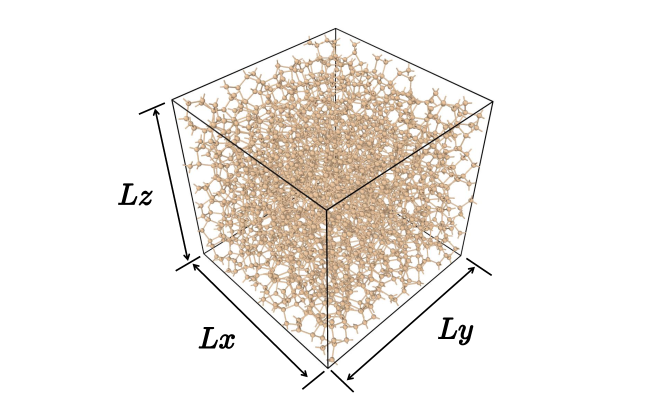
As shown in Fig. 1, we perform our simulations in the periodic and cuboid simulation box $L_{x}$$\times$$L_{y}$$\times$$L_{z}$ in the $x$-, $y$- and the $z$-directions respectively. These are however not fixed quantities, but are allowed fluctuate when the bond transpositions are made as the sample evolves in time.

Throughout this paper, we consider three geometric quantities, defined as follows:

$$V(t) = L_{x}(t)L_{y}(t)L_{z}(t),$$

$$B_{1}(t) = L_{y}(t)/L_{z}(t),$$

$$B_{2}(t) = L_{y}(t)L_{z}(t)/L_{x}^{2}(t).$$ (3)

Figure 3: (color online) (a) Typical fluctuations of $V$, $B_{1}$ and $B_{2}$ (from top to bottom) evolved up to 5$\times 10^{6}$ Monte Carlo steps (MCS) for a sample with $N=423$ atoms under $T=1400$K. While, given enough time, $B_{1}$ and $B_{2}$ can take a wide range of values, $V$ will only show fluctuations around its ideal value which is set by the density of the a-Si sample. The inset in the bottom panel exhibits stalling events (see text for details). (b) Measurements of the MSD for $V$, $B_{1}$ and $B_{2}$ respectively . $B_{1}$ and $B_{2}$ are multiplied by $10^{6}$ to have the same scale as $V$. The results are obtained from averaging over 10 starting samples with 423 atoms ($T=1400$K), each evolved 50 times with different random seeds over $10^{7}$ proposed bond transpositions to achieve a good statistical performance, which offset the noise generated by a single evolution. At short times, all three curves of the MSD initially increase linear in time, i.e. show ordinary diffusion. After $\sim 10^{4}$ attempted bond transpositions, the increase slows down significantly. All curves show a crossover to subdiffusive behavior. For the MSD_V we expect eventually saturation; this seems to be at times beyond those of our simulations.

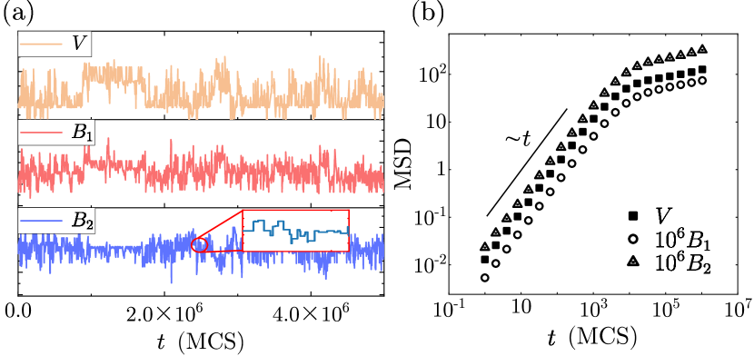
Physically, for a cuboid sample such as ours, the dynamics of shape fluctuations of the sample can be efficiently characterized by associating $V(t)$ to the dynamics of the “bulk” mode, and $B_{1}(t)$ and $B_{2}(t)$ with that of the “shear” modes. Fig. 3(a) shows the trajectories for these quantities in Monte-Carlo time at short times. The stalling events seen therein (inset, Fig. 3(a)) result from the rejected bond transpositions at short time intervals. Figure 3(b) displays the MSD for $V$, $B_{1}$ and $B_{2}$, respectively. At short times, there are only few bond transpositions which occur at spatially separated locations, and thus these are uncorrelated events, which yield normal diffusive behavior. At longer times, this spatial separation breaks down, and the bond transpositions start to feel each other; for instance, a bond transposition which leads to local contraction has an enhanced probability to be followed by another bond transposition that leads to local expansion. The cross-over point represents the transition from normal diffusion to anomalous diffusion of the physical quantity under study.

3.1 Diffusive behavior at short times

At short times, we track the dynamics of shape fluctuations of the samples in terms of the mean-square displacements MSD${}_{V}(t)=\langle[V(t)-V(0)]^{2}\rangle$, MSD${}_{1}(t)=\langle[B_{1}(t)-B_{1}(0)]^{2}\rangle$ and MSD${}_{2}(t)=\langle[B_{2}(t)-B_{2}(0)]^{2}\rangle$, with the angular brackets denoting ensemble averages for a sample of fixed number of atoms and (more or less) constant energy. As shown in Fig. 3(b), At short times, all three quantities exhibit ordinary diffusive behavior, i.e. MSD($t$)$\sim t$. $V$ is expected to saturate after super long times due to the constraint of structural density, while significant crossovers (nearly at $10^{4}$) to sub-diffusion can be observed in MSD${}_{1}(t)$ and MSD${}_{2}(t)$ i.e. MSD($t$) $\sim t^{\alpha}$ ($\alpha<1$). Here the results are obtained from averaging 10 starting samples ($N=423$) each evolved 50 times.

$$\mbox{MSD}(t)=2Dt.$$ (4)

By fitting the MSD for $V$, $B_{1}$ and $B_{2}$ we extract the corresponding diffusion coefficients $D$. Since $V$, $B_{1}$ and $B_{2}$ all bear relations to $L_{x}$, $L_{y}$ and $L_{z}$, one would expect them to be related through these length parameters, which we establish below. In order to do so, having denoted the change in $V$, $B_{1}$ and $B_{2}$ over a small time interval $dt$ for samples with dimensions $L_{x}$ and $L_{y}$ by $dV$, $dB_{1}$ and $dB_{2}$ respectively, we express them in terms of small changes $dL_{x}$, $dL_{y}$ and $dL_{z}$ as

$$\langle dV^{2}\rangle\!\!\! = \!\!\!\left\langle\!\left[L_{y}L_{z}dL_{x}+L_{z}L_{x}dL_{y}+L_{x}L_{y}dL_{z}\right]^{2}\right\rangle$$

$$\langle dB^{2}_{1}\rangle\!\!\! = \!\!\!\left\langle\!\frac{1}{L_{z}^{4}}\!\left[L_{z}dL_{y}-L_{y}dL_{z}\right]^{2}\!\right\rangle\quad\mbox{and}$$

$$\langle dB^{2}_{2}\rangle\!\!\! = \!\!\!\left\langle\!\frac{1}{L_{x}^{6}}\!\left[L_{x}L_{y}dL_{z}+L_{z}L_{x}dL_{y}-2L_{y}L_{z}dL_{x}\right]^{2}\!\right\rangle\!\!.$$ (5)

Numerically, we find that cross-terms such as $\langle dL_{x}dL_{y}\rangle$ etc. are much smaller than terms like $\langle dL_{x}^{2}\rangle$. Similarly, it can be argued that thermal kicking on a sample acts like a force in the $x$-, $y$- and $z$- directions as stretching forces, and the sample cannot distinguish among the three directions. In particular, if the condition holds that the extension of the sample along the $x$-direction is inversely proportional to the corresponding spring constant $(L_{y}L_{z})^{-1}$, then $\langle dL_{x}^{2}\rangle\sim(L_{y}L_{z})^{-2}$ etc. These two assumptions lead to the following scaling relations between the diffusion coefficients:

$$D_{V}/D_{B_{1}}\propto\left\langle{L_{x}^{2}L_{z}^{4}}\right\rangle$$

$$D_{B_{1}}/D_{B_{2}}\propto\left\langle{L_{x}^{4}/L_{z}^{4}}\right\rangle$$

$$D_{V}/D_{B_{2}}\propto\left\langle{L_{x}^{6}}\!\right\rangle.$$ (6)

Figure 4: (a)-(c) Double logarithmic plots showing the relations between any two of the diffusion coefficient of the quantities we construct, which are built through statistical value of the lateral lengths. ${D_{V}}\sim{\alpha_{1}}\langle{L_{x}^{2}}{L_{z}^{4}}\rangle{D_{B_{1}}}$, ${D_{V}}\sim{\alpha_{2}}\langle{L_{x}^{4}}\rangle{D_{B_{2}}}$, ${D_{B_{1}}}\sim{\alpha_{3}}\langle{L_{x}^{4}}/{L_{y}^{4}}\rangle{D_{B_{2}}}$, here $\alpha_{1}$, $\alpha_{2}$ and $\alpha_{3}$ are constants and numerically obtained from our simulations as: 0.0584, 0.3302 and 0.0195, respectively

The numerical results are shown in the Fig. 4, the diffusion coefficients (corresponding to the short time part in the Fig. 3(b)) are measured according to the Eq. 4, the four data points in each plots are measured over $N=423,1000,1500$ and $2000$. Data is collected by averaging over 10 initial samples, each evolved 50 times over $10^{7}$ proposed bond transpositions. It is numerically found that ${D_{V}}\sim{\alpha_{1}}\langle{L_{x}^{2}}{L_{z}^{4}}\rangle{D_{B_{1}}}$, ${D_{V}}\sim{\alpha_{2}}\langle{L_{x}^{6}}\rangle{D_{B_{2}}}$, ${D_{B_{1}}}\sim{\alpha_{3}}\langle{L_{x}^{4}}/{L_{z}^{4}}\rangle{D_{B_{2}}}$, the factors $\alpha_{1}$, $\alpha_{2}$ and $\alpha_{3}$ are constant and fitted from our simulations: 0.0584, 0.3302 and 0.0195, respectively, we infer that these values are more likely to depend on factors such as sample size, amount of data, measurement time length, system noise, etc., which can be used as references in future experiments.

3.2 Characterizing material dynamics at long times

In comparison to the short time dynamics, the dynamics at long times is much more noisy, simply because obtaining very long time series for an a-Si sample is not easy. Just to give an idea, a run on a single core of Intel i7-9700k CPU, our simulations require 0.005s/step for a sample with 1000 atoms for $T=1500$K. Given that the crossover event often takes place at $10^{4}$ steps, at least $10^{6}$ steps, and averaging over 50 independent sample runs, costing five days, would be required for obtaining results with good statistics (larger samples and lower temperatures would require even longer times.) To complicate matters, we also have to deal with the stalling events. Fortunately, we have found a way to go around the complications due to the stalling events, as described in Sec. 3.2.1 below.

3.2.1 Stalling events complicate handling of time-series data

Figure 5: (a) Waiting time distribution fitted to Eq. (7) for $N=423$ at various temperatures (up to $\tau_{w}=$3,000), inset: fit for lager scales (up to $\tau_{w}=$20,000). (b) Monte Carlo time $t$ for a sample with $N=423$, measured in the number of proposed bond transpositions, in comparison with the event time $\tau$, measured in the number of accepted bond transpositions. Each dot in this scatter plot is a measurement of both times, elapsed between accepted bond transpositions. The data show a linear relation between $t$ and $\tau$, with a temperature-dependent scale factor. As is to be expected, there is some spread in the data points at short times, which decreases with increasing times.

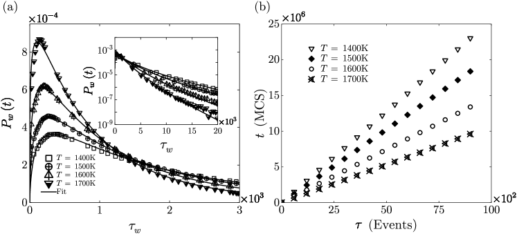
The stalling events pose us with a difficulty on how to cleanly handle the dynamics data at long times: specifically, $V$, $B_{1}$ and $B_{2}$ changing only at irregular time intervals means that ensemble averages, calculated standardly from time-series data, is bound to be very noisy (it is!) at long times. Stalling events are a manifestation of the MC procedure: over a stalling period, which is synonymous to a waiting time (i.e., the sample configuration is waiting for a change), all proposed bond transposition events in the MC procedure are rejected. That said, the stalling events also provide us with the opportunity to measure time in units of accepted bond transposition moves, $\tau$, instead of the standard units of MC time $t$, measured in units of attempted bond transposition moves. Clearly, the quantity $\tau$ increases by unity at every accepted move, even though the MC time between two successive accepted moves, the waiting time can be widely different due to stochasticity of the process. Indeed, when measured in units of $\tau$, we find that the dynamical quantities at long times are far less noisy, and for this reason, throughout this section we measure time in units of $\tau$.

But before we get to the dynamics, we present the probability distribution of the waiting time $P_{w}(t)$ in Fig. 5(a) for a sample with $N=423$ and a couple of different temperature values. Plotting the data in log-linear plot, and subsequent analysis, reveals that the $P_{w}(t)$ data are well fitted by the following formula:

$$P_{w}(t)=at^{b}e^{-(\tau_{w}/\tau_{c})^{d}},$$ (7)

where $a$ is a normalization constant. The fitting parameters are noted in Table 1. In particular, we note that the waiting time distributions do not have power-law tails. We will return to this aspect later in this section. Moreover, in Fig. 5(b) we also show that the mean waiting time is a constant throughout the duration of the simulation (the constant corresponds to the inverse rate of the accepted moves).

Table 1: Parameters for the fitted waiting time distribution in Fig. 5(a).

Temperature (K)	$a$	$b$	$\tau_{c}$	$d$
1400	2.070 $\times 10^{-5}$	0.767	125.000	0.474
1500	4.721 $\times 10^{-5}$	0.615	195.100	0.525
1600	1.179 $\times 10^{-4}$	0.466	274.800	0.595
1700	3.315 $\times 10^{-4}$	0.300	350.000	0.667

3.2.2 Anomalous diffusion of $V$, $B_{1}$ and $B_{2}$

Figure 6: (color online) (a)-(c) Measurement of the exponent $\alpha$ in log($\tau$) scale for various temperatures with fixed $N=423$. $\alpha$ is smaller then 1 throughout the entire time, which indicates a subdiffusive behavior for the corresponding mean-square displacement. After an initial period of crossover time, $\alpha$ eventually converges to a small value (0.1-0.3). (d) The anomalous exponent (as defined in Eq. 8) as obtained from the MSD of $B_{1}$, $B_{2}$ and $V$, as a function of temperature. At higher temperatures, the values of $\alpha$ obtained from the MSD of $V$ are lower than those for $B_{1}$ and $B_{2}$, probably because large deviations of the density away from the crystalline value are suppressed (as discussed in the text).

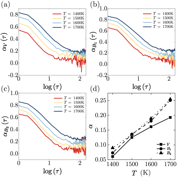
Double logarithmic plots of the mean-square displacements reveal that the dynamics of $V$, $B_{1}$ and $B_{2}$ is no longer diffusive, i.e., they are anomalous, at long times. Assuming that the $\text{MSD}_{V}(\tau)$, $\text{MSD}_{B_{1}}(\tau)$ and $\text{MSD}_{B_{2}}(\tau)$ increase as a power-law in $\tau$ at long times, we compute the effective exponents for these variables, collectively denoted by $Q$, as

$$\alpha_{Q}\left(\tau\right)=\frac{d\log\left[\text{MSD}_{Q}\right]}{d\log\tau}.$$ (8)

An example plot for $\alpha_{Q}$ is shown for $N=423$ in Fig. 6(a)-(c) above. The exponents we find are dependent on temperature (shown in Fig. 6(d)). It seems to us that lower temperature leads to lower subdiffusion exponent, even though measuring exact exponents properly is difficult given long run times. The approximate exponents for each quantities at various temperature are list in Tab. 2.

Table 2: The anomalous diffusive exponent $\alpha$ for $V$, $B_{1}$, and $B_{2}$ with fixed $N=423$ and various $T$.

Quantity	$T$ (K)	$\boldsymbol{\alpha}$
$V$	1400	0.06
$V$	1500	0.13
$V$	1600	0.16
$V$	1700	0.20
$B_{1}$	1400	0.07
$B_{1}$	1500	0.14
$B_{1}$	1600	0.18
$B_{1}$	1700	0.25
$B_{2}$	1400	0.09
$B_{2}$	1500	0.13
$B_{2}$	1600	0.19
$B_{2}$	1700	0.25

3.2.3 Further analysis of anomalous diffusion

Long runtimes required to obtain long time series of sample snapshots prevent us to pinpoint the exponents with higher numerical accuracy. Nevertheless, we can still reflect on the nature of the anomalous diffusion we observe here for a-Si. In particular, in the past work of two of us, we have observed that anomalous diffusion in materials tend to belong to the fractional Brownian motion (fBm) class, while their stochastic dynamics described by Generalized Langevin equation (GLE) with power-law memory [17, 18, 19, 20], with the exponent of the power-law memory, within the numerical accuracy, matching the anomalous diffusion exponent really well. The memory can be interpreted in terms of restoring forces: when thermal fluctuations move a sample configuration one way, subsequent fluctuations tend to undo that move. If the simulations of a-Si were amenable to reach sufficiently long times, we would be able to perform a similar analysis here as well; unfortunately that is not the case.

$$C_{v}^{Q}\left(\tau\right)=\frac{\left<v_{Q}\left(\tau\right)v_{Q}\left(0\right)\right>}{\left<\left(v_{Q}\left(0\right)\right)^{2}\right>}.$$ (9)

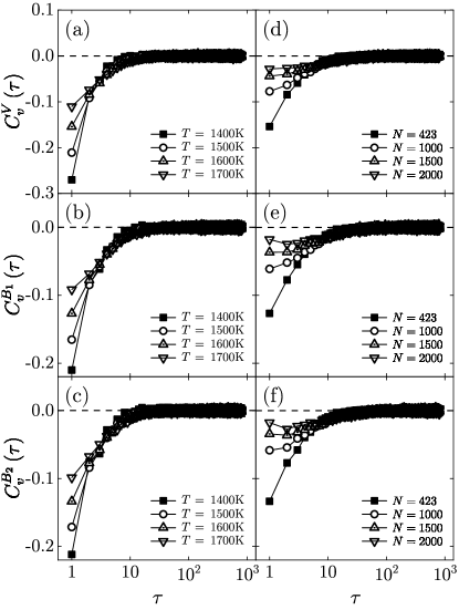
That said, given that the waiting times do not have a power-law tail, as demonstrated in Fig. 5 rules out a continuous-time random walk (CTRW) type stochastic process for $V$, $B_{1}$ and $B_{2}$. To completely rule out CTRW, we plot the velocity autocorrelation function (VACF) for these quantities in Fig. 7, VACF $C_{v}^{Q}\left(\tau\right)$ is defined in Eq. 9 for quantity $Q$, where $v_{Q}\left(\tau\right)=\partial Q/\partial\tau$ is the velocity of the quantity Q. These data rather cleanly demonstrate that the VACF is negative for $\tau\neq 0$, and approaches zero for large $\tau$ from below the $x$-axis.

Figure 7: Normalized velocity auto-correlation functions (VACF) of $V$, $B_{1}$ and $B_{2}$ for various temperatures with fixed $N=423$ (a)-(c) , and (d)-(f) for various the number of atoms with a fixed temperature of 1500K. The VACF are clearly negative at very short times, indicating that there is a restoring tendency: if in one bond transposition, the sample shears one way, the following bond transposition has a bias in favor of undoing the earlier shear. It also implies the autocorrelation is weaker for a larger system.

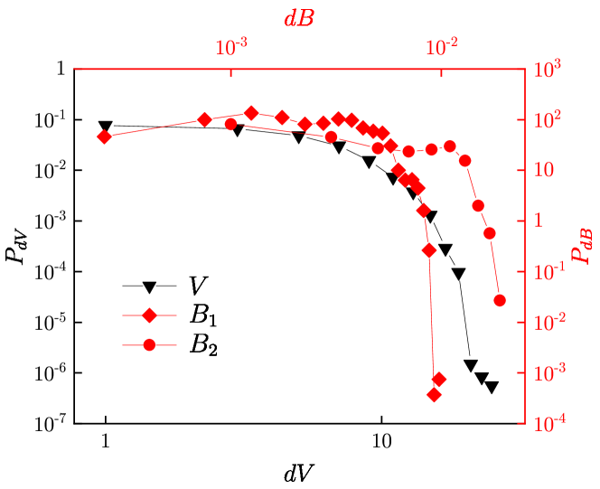
For completeness, we also present the jump length distributions of $B_{1}$, $B_{2}$ and $V$ in Fig. 8. Note that these distributions do not feature fat tails, thereby ruling out Levy-flight like effects.

4 Discussion

Figure 8: (color online) Double logarithmic plots of the jump length distribution for $B_{1}$, $B_{2}$ and $V$ ($N=423$, $T=1500$K). None of these distributions feature fat (power-law) tails, thereby ruling out Levy-flight behavior.

This manuscript studies the structural dynamics of a model of amorphous silicon, in particular the fluctuations in the volume $V$ of the simulation box, as well as in its aspect ratios $B_{1}$ and $B_{2}$. The simulations show that these three variables show ordinary diffusive behavior at very short times, crossing over to anomalous diffusion at longer times: their MSDs can be well fitted with a power-law MSD$\sim t^{\alpha}$ with $\alpha<1$. We find that the anomalous exponent $\alpha$ is temperature-dependent.

Various models in statistical physics exist that also feature anomalous dynamics; two well-known examples are the continuous time random walker (CTRW) and fractional Brownian motion (fBM). In further investigation, we present the distribution of the waiting times, as well as the velocity autocorrelation functions. These further results show that the observed anomalous dynamics is consistent with fBM-like behavior, and not with CTRW-like behavior.

The observed fluctuations in the shape of the simulation cell are directly related to deformations of the material under external compression and shear forces. Our findings are therefore directly linked to experiment.

References

- [1] Jeffrey L Braun, Christopher H Baker, Ashutosh Giri, Mirza Elahi, Kateryna Artyushkova, Thomas E Beechem, Pamela M Norris, Zayd C Leseman, John T Gaskins, and Patrick E Hopkins. Size effects on the thermal conductivity of amorphous silicon thin films. Physical Review B, 93(14):140201, 2016.
- [2] Wu-Xing Zhou, Yuan Cheng, Ke-Qiu Chen, Guofeng Xie, Tian Wang, and Gang Zhang. Thermal conductivity of amorphous materials. Advanced Functional Materials, 30(8):1903829, 2020.
- [3] Frederik Tielens, Maciej Gierada, Jarosław Handzlik, and Monica Calatayud. Characterization of amorphous silica based catalysts using dft computational methods. Catalysis Today, 354:3–18, 2020.
- [4] Xiaoning Ru, Minghao Qu, Jianqiang Wang, Tianyu Ruan, Miao Yang, Fuguo Peng, Wei Long, Kun Zheng, Hui Yan, and Xixiang Xu. 25.11% efficiency silicon heterojunction solar cell with low deposition rate intrinsic amorphous silicon buffer layers. Solar energy materials and solar cells, 215:110643, 2020.
- [5] Shuangying Cao, Dongliang Yu, Yinyue Lin, Chi Zhang, Linfeng Lu, Min Yin, Xufei Zhu, Xiaoyuan Chen, and Dongdong Li. Light propagation in flexible thin-film amorphous silicon solar cells with nanotextured metal back reflectors. ACS applied materials & interfaces, 12(23):26184–26192, 2020.
- [6] Mengxiao Huang, Yunfeng Wang, Ming Li, Vanhkeo Keovisar, Xuejuan Li, Decheng Kong, and Qiongfen Yu. Comparative study on energy and exergy properties of solar photovoltaic/thermal air collector based on amorphous silicon cells. Applied Thermal Engineering, 185:116376, 2021.
- [7] Van-Thuc Nguyen and Te-Hua Fang. Abrasive mechanisms and interfacial mechanics of amorphous silicon carbide thin films in chemical-mechanical planarization. Journal of Alloys and Compounds, 845:156100, 2020.
- [8] 9_F Wooten, K Winer, and D Weaire. Computer generation of structural models of amorphous si and ge. Physical review letters, 54(13):1392, 1985.
- [9] PN Keating. Effect of invariance requirements on the elastic strain energy of crystals with application to the diamond structure. Physical Review, 145(2):637, 1966.
- [10] GT Barkema and Normand Mousseau. Identification of relaxation and diffusion mechanisms in amorphous silicon. Physical review letters, 81(9):1865, 1998.
- [11] Mark D Kluge, John R Ray, and Aneesur Rahman. Amorphous-silicon formation by rapid quenching: A molecular-dynamics study. Physical Review B, 36(8):4234, 1987.
- [12] Federico D’Ambrosio, Joris Barkema, and Gerard T Barkema. Efficient structural relaxation of polycrystalline graphene models. Nanomaterials, 11(5):1242, 2021.
- [13] Nicholas Metropolis, Arianna W Rosenbluth, Marshall N Rosenbluth, Augusta H Teller, and Edward Teller. Equation of state calculations by fast computing machines. The journal of chemical physics, 21(6):1087–1092, 1953.
- [14] Julien Guénolé, Wolfram G Nöhring, Aviral Vaid, Frédéric Houllé, Zhuocheng Xie, Aruna Prakash, and Erik Bitzek. Assessment and optimization of the fast inertial relaxation engine (fire) for energy minimization in atomistic simulations and its implementation in lammps. Computational Materials Science, 175:109584, 2020.
- [15] Gerard T Barkema and Normand Mousseau. High-quality continuous random networks. Physical Review B, 62(8):4985, 2000.
- [16] Zihua Liu, Debabrata Panja, and Gerard T Barkema. Structural dynamics of polycrystalline graphene. Physical Review E, 105(4):044116, 2022.
- [17] Debabrata Panja. Generalized langevin equation formulation for anomalous polymer dynamics. Journal of Statistical Mechanics: Theory and Experiment, 2010(02):L02001, 2010.
- [18] Debabrata Panja. Anomalous polymer dynamics is non-markovian: memory effects and the generalized langevin equation formulation. Journal of Statistical Mechanics: Theory and Experiment, 2010(06):P06011, 2010.
- [19] Wei Zhong, Debabrata Panja, Gerard T Barkema, and Robin C Ball. Generalized langevin equation formulation for anomalous diffusion in the ising model at the critical temperature. Physical Review E, 98(1):012124, 2018.
- [20] Debabrata Panja, Gerard T Barkema, and JMJ van Leeuwen. Efficient simulation of semiflexible polymers. Physical Review E, 92(3):032603, 2015.