Modular Safety-Critical Control of Legged Robots*
Abstract
Safety concerns during the operation of legged robots must be addressed to enable their widespread use. Machine learning-based control methods that use model-based constraints provide promising means to improve robot safety. This study presents a modular safety filter to improve the safety of a legged robot, i.e., reduce the chance of a fall. The prerequisite is the availability of a robot that is capable of locomotion, i.e., a nominal controller exists. During locomotion, terrain properties around the robot are estimated through machine learning which uses a minimal set of proprioceptive signals. A novel deep-learning model utilizing an efficient transformer architecture is used for the terrain estimation. A quadratic program combines the terrain estimations with inverse dynamics and a novel exponential control barrier function constraint to filter and certify nominal control signals. The result is an optimal controller that acts as a filter. The filtered control signal allows safe locomotion of the robot. The resulting approach is generalizable, and could be transferred with low effort to any other legged system.
I Introduction
As in nature, legs enable robots to travel in challenging environments such as rough terrain, to climb stairs, and to reach tight spots. The next step for legged robots is integrating them further into daily lives with an emphasis on safety.
In the scope of this work, we consider the safety of a legged robot as maintaining its ability to locomote; it can be also stated simply but roughly as not falling. It must be noted that there is no concrete definition of safe locomotion as there is no agreed way of quantifying safety [1, 2].
I-A Related Work
In current literature, the stability of legged robots is considered for flat ground. However, this assumption is often violated; the point of having legs is to clear rough terrain. As a solution, some recent work focused on estimating the effect of the terrain [3]. Others [4, 5] have shown only proprioceptive, i.e., blind, measurements combined with deep learning are effective in considering terrain effects. However, there has been no work on a dedicated proprioceptive terrain estimator. In this study, we propose a method such that the robot gains access to the terrain properties with no additional sensors. With the proposed approach, only the sensors required to control a robot should suffice; thus reducing the cost and complexity due to sensors like cameras and lidars.
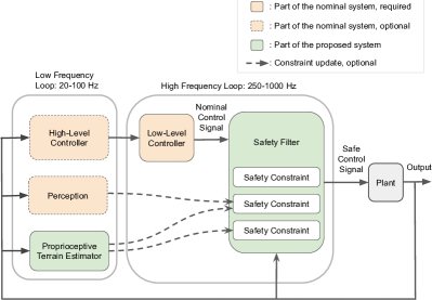
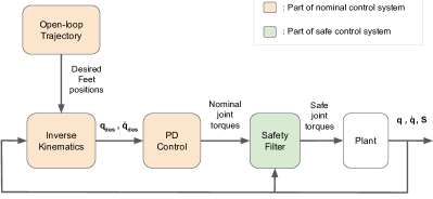
Another recent development is the introduction of the control barrier function (CBF) framework to guarantee the safe operation of dynamic systems such as legged robots [6]. Our work uses the CBF framework to generate constraints such that rough terrain can be safely navigated. The terrain can be estimated by the previously described blind terrain estimator, and fed into the constraints to generate an adaptive safety filter. The resulting system will function as a filter, allowing it to be integrated easily as shown in Figure 1.
Some of the most impressive, high-performance controllers are obtained with reinforcement-learning methods [5]. However, learning-based controllers are based on simple models or no model at all, i.e., model-free. Combining such controllers with model-based safety constraints would be an effective way to address safety concerns. Thus, our proposed safety filter would be especially valuable in the testing and eventual deployment of learning-based systems.
I-B Contributions
In this work, the following three contributions are made:
-
•
An intuitive, high-level optimal-control-based safety filter framework is implemented with direct support for the CBF framework. The source code is publically available [7].
-
•
The transformer architecture from deep learning is adapted to model terrain friction using only proprioceptive measurements.
-
•
A novel exponential control barrier function (ECBF) is formulated and implemented for ground clearance of the swing foot of legged robots.
II Background
II-A Dynamics of a Legged Robot
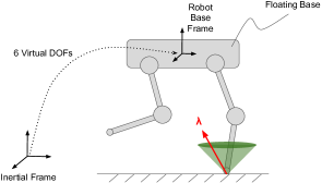
A legged robot, as shown in Figure 2, is an underactuated control system [8]. Define as the number of actuated joints and as the number of unactuated joints. The total DoF is defined as . Underactuation implies ; robot control must be achieved through contact.
In the scope of robot dynamics [9, 10], contact is commonly modeled as rigid point contacts. For legged robots, which make and break contact in various combinations, a popular choice is to use excess coordinates. In this case, a link is selected as the floating base; then the floating base frame and an inertial frame are connected through 6 virtual, unactuated DoFs (degrees-of-freedom), . The resulting equation allows us to represent the dynamics concisely:
| (1) |
where
-
•
is the robot configuration vector which includes both actuated and unactuated DoFs; .
-
•
is the robot velocity, .
-
•
is the robot accelerations.
-
•
is the control inputs, i.e., joint torques.
-
•
is the mass matrix.
-
•
is the nonlinear effects: centrifugal, Coriolis, and gravity terms.
-
•
is the selection matrix, .
-
•
is the contact jacobian transposed. Define as the number of contact points. For each contact point, there will be a 3D constraint force.
-
•
is the vector of constraint forces. It is updated whenever there is a change in the contact states.
-
•
is the vector of forces applied on the robot DoFs due to contact. It is the only term to control .
II-B Quantifying Safety: Viability
For traditional control systems, stability is analyzed by established measures such as eigenvalues or phase margins. Legged robots require special attention due to the complexity of quantifying the robot’s safety. Safe locomotion of legged robots is seen as a problem of viability instead of Lyapunov stability [11, 2].
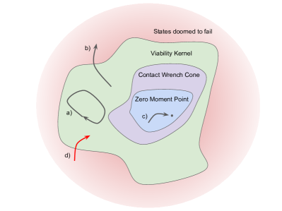
The viability kernel is defined as the set of all states where the system remains safe, i.e., it can keep operating. By definition, any state that is out of the viability kernel cannot return to the viability kernel, and thus it eventually ends up in a failed state. Figure 3 illustrates this via examples.
II-C Control Barrier Functions
The CBF framework [6] lends itself to the synthesis of controllers which possess set forward invariance. As a model-based approach, it enables theoretical guarantees by checking and restricting derivatives. Define the system states as , where is the entire state space of the system. Then a CBF, , is defined so that returned scalar value must always be positive for safe states, i.e., safe if . The framework allows the construction of linear inequality constraints that can be used in optimal controllers.
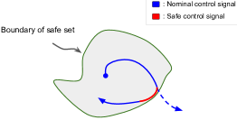
As shown in Figure 1, the CBF framework is commonly used as a safety filter that can be inserted into an existing control system after the nominal controller. In a quadratic program (QP), we can include linear inequality constraints allowing us to formulate a CBF-QP safety filter. The safety filter is minimally intrusive, i.e., it will only interfere with the nominal control signal near the boundary of the safe set to make sure the system remains in the safe states, which is illustrated in Figure 4.
II-D Terrain Estimation with Spatial-Temporal Data
To model the motion of agents, e.g., skeleton-based action recognition, it is common to use joint measurements, such as 3D coordinates, to construct a graph [15]. The quantities for each joint at each time step are represented as a node in the graph. Since the nodes are distributed over both spatial and temporal dimensions, connecting the nodes results in a spatial-temporal model. Such graphs can be processed by machine learning models.
Transformer architecture has retained its popularity in deep learning since its introduction by [16]. The self-attention of the transformer gives it its expressive power, but it is costly to compute. Its limitation of modeling long sequences can be overcome with efficient transformers [17, 18].
Previous work has shown that it is possible to estimate terrain properties by only using proprioceptive measurements [19]. Their analysis shows that the model can accurately reconstruct the terrain. With terrain properties, two important ones affecting the robot dynamics are meant: friction coefficient and a rough estimate of the elevation map of the terrain, i.e., macroscopic surface roughness.
III Modular Safety-Critical Control
III-A Inverse Dynamics Formulation with CBF Constraints
To implement a safety filter, one can use the CBF-QP formulation [6]. In that case, we must embed the dynamics into the barrier inequality constraints. This requires two undesirable operations: inversion of the mass matrix and solving for [20]. Finding is challenging; it requires the assumption that kinematic contact constraints are satisfied. Inversion of the mass matrix tends to get numerically stiff [21]. Thus, it is preferable to have an inverse dynamics formulation without these issues. Following [22], we achieve the following formulation, which will be called ID-CBF-QP:
| (2) | |||
| (3) | |||
| (4) | |||
| (5) | |||
| (6) | |||
| (7) | |||
| (8) | |||
| (9) |
where
-
•
Equation (2) is the objective function. Three different decision variables, concatenated into vector , will be optimized. The decision variables are:
-
1.
, accelerations for all degrees of freedom,
-
2.
, torques for actuated joints,
-
3.
, concatenated ground reaction forces from each contact point.
-
1.
- •
-
•
Stance feet must maintain their contact mode; it can be done by including friction cone constraints:
-
1.
Equation (5) is the unilateral contact constraint to avoid loss of contact for each stance foot, foot .
- 2.
-
1.
-
•
Equation (8) is the control barrier constraint.
-
•
Equation (9) is the joint torque limits.
III-B Ground Clearance Enforced by an ECBF
As an inequality constraint, we can incorporate CBFs into the optimization problem, as shown in (8). There can be multiple CBF constraints as long as the QP remains feasible. In this instance, we define a novel CBF constraint to keep the feet from hitting the ground by including the terrain profile.
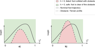
We apply an ECBF to enforce ground-clearance of the robot’s end-effectors, i.e., its swing feet; so that its feet do not hit obstacles or adepts to uneven terrain while walking. Figure 5 describes the constraint by illustrating two sample cases. We start the formulation with a position-based CBF:
| (10) |
where is the phase variable, denoting the progress of the swing phase; is the z-axis position (height) of the th swing foot in the world frame; maps the phase variable to desired ground-clearance height for the th swing foot in the world frame. can be thought as the obstacle heights over the gait period.
To use the ECBF approach, we need and its derivatives. In this work, we define the phase variable, as follows:
| (11) |
where is time. Its time derivates are given by:
| (12) | |||
| (13) |
Since the ground-clearance CBF, , is a position-based CBF, it cannot be directly used [23]. We encounter a control barrier function for a second relative degree safety constraint. We solve this problem by using the generalized formulation, ECBF. To employ the ECBF approach we define an auxiliary function, :
| (14) |
Then, the ECBF constraint is:
| (15) |
Taking the derivatives and substituting, we get:
| (16) |
With the help of , Jacobian of the flight feet, we recover one of the optimization variables; :
| (17) |
Note, the ECBF constraint, (15), does not directly include the control signal, . However, the CBF framework requires in the final constraint. Equation (15) can serve as a valid CBF because, appears in affine relation to in (3) [22].
| Parameter | Value |
| dt | 0.03 s |
| Number of timesteps | 40 |
| Total time | 1.2 s |
| Number of environments (robots) | 4096 |
| Number of features per timestep | 36 |
We use readily available, highly optimized QP solvers; as long as the inequality constraint is written in the standard form, we can use any off-the-shelf solver:
| (18) |
where is the linear inequality matrix, is the linear inequality vector. Reorganizing (17) to match the format of (18), we get the inequality constraint in the standard form:
| (19) |
where we add one row for each foot in flight; since is a row vector.
IV Data-Based Terrain Estimator
IV-A Network Architecture
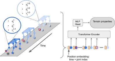
Section II-D discussed the existing literature on modeling terrain with machine learning. In this section, we propose a new approach in the same vein. Instead of constructing a sparse graph manually, we use a dense graph in which every node is connected. It is possible to achieve such a model using Transformer architecture [16]. In this sense, each node in the graph becomes a token. The tokens are constructed by combining the proprioceptively available measurements: joint positions, , joint velocities, , joint torques, . The full attention mechanism is not suited for long sequences. Instead, we use one of the efficient transformers, Linformer [18]. Linformer reduces the complexity to , allowing us to use it for long sequences with little loss of expression.
The proposed network is illustrated in Figure 6. Network architecture draws heavy inspiration from the vision transformer [24]. Measurements of the joint quantities over a time window are concatenated with learned spatial-temporal position embeddings and fed into the network. Using such a model, terrain estimations can be provided to the ID-CBF-QP described in Section III-A: Friction cone constraints, (6) and (7), can be improved by updating ; CBF ground-clearance constraint, (8), can be improved by updating in (10).
IV-B Data Collection
To train the terrain estimation model described in the previous section, large amounts of data are required. We use Nvidia Omniverse Isaac [25], a GPU-accelerated simulator that can achieve an order of faster simulations than the common CPU-based simulators.
Building on the work of [26], we can use Nvidia Isaac to simulate and gather data for legged robots. A simulation with 4096 parallel Unitree A1 quadrupeds reaches 100,000 steps per second on an Nvidia RTX 3080 12GB GPU. We record the simulation observations to create a dataset. Table I displays the refined input for the model.
V Quadruped Implementation
We have implemented a software package to work on mechanical systems via optimal control [7]. Our software package uses PyBullet [27] for simulation and Pinocchio [28] for rigid body computations. PyBullet is used only for simulation and observation; all calculations are carried out via Pinocchio. This enables an easy transition to an actual robot, where highly efficient and embedded-ready Pinocchio is fully utilized. To solve the ID-CBF-QP, we use OSQP [29].
The selected quadruped robot is Unitree A1, it has 12 actuated joints, 3 for each leg; it weighs 12 kilograms. The nominal controller, shown in Figure 7, achieves a trotting gait with open-loop feet trajectories.
VI Results and Discussion
VI-A Friction Cone
The ground reaction forces predicted by the ID-CBF-QP from Section III-A are close to the actual values from the simulation: the vertical component has a mean absolute error of 3.051 N; the lateral components have a mean absolute error of 1.847 N.
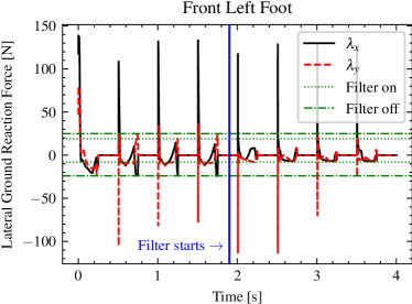
To demonstrate the effectiveness of the friction constraint, a low friction value is set for the constraints: . The resulting control and ground reaction forces are shown for an arbitrarily selected foot in Figure 8. In the figure, only the lateral forces are shown to keep it comprehensible. Since our nominal controller uses inverse kinematics, it does not take forces into account. We compute inverse dynamics and apply friction cone constraints by introducing the safety filter; thus, allowing us to eliminate foot sliding and enable safer locomotion.
VI-B Ground Clearance
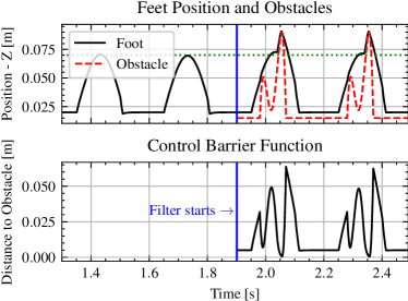
Figure 9 shows the simulation results in the presence of the ground-clearance constraint from Section III-B. In the figure, we observe that the ECBF framework works as expected and keeps the foot clear of the obstacle with minimal interference to the nominal control signal. We have used a polynomial for demonstration. However, this is not necessary because our formulation only requires the obstacle profile to be twice differentiable. ID-CBF-QP can become infeasible for aggressive obstacle profiles due to limited joint torques.
VI-C Terrain Estimator
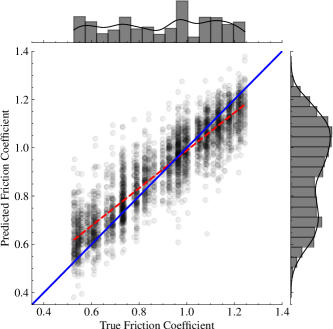
The model can predict the friction coefficient with a mean absolute error of 0.0720 using randomly sampled 3264 data points from the test split. Figure 10 shows the regression performance of the predictions. In our work, we obtained the good results using data from a range of 0.6-2 seconds. In such time spans, there are hundreds of tokens. This justifies using efficient transformers to model them as long sequences.
VII Conclusion and Outlook
This study presents a novel approach to safety-critical control of legged robots. We have developed a flexible optimal control software package for legged robots. We have included several safety criteria by defining constraints for the optimization problem. They cover some of the major sources of locomotion failures. In addition, we have developed a machine-learning model to estimate terrain properties using proprioceptive sensors. The developed terrain estimator can be added to most robots to increase their contact awareness which can then be used for high-performance control.
Our work is limited to simulation. Experimental work would be beneficial in the future. Thus, intentional or unintentional simplifications from the simulation could be verified and fixed. The terrain estimator could be extended to height map estimation as a future work. Also, there is no established method to evaluate the performance of legged robots; therefore a locomotion benchmark would accelerate progress in the field. Furthermore, improved definitions of locomotion safety, especially ones with a probabilistic sense would be valuable.
References
- [1] Y. Gong and J. W. Grizzle, “Zero dynamics, pendulum models, and angular momentum in feedback control of bipedal locomotion,” Journal of Dynamic Systems, Measurement, and Control, vol. 144, no. 12, p. 121006, 2022.
- [2] P. Zaytsev, W. Wolfslag, and A. Ruina, “The boundaries of walking stability: Viability and controllability of simple models,” IEEE Transactions on Robotics, vol. 34, no. 2, pp. 336–352, 2018.
- [3] J. Carpentier and N. Mansard, “Multicontact locomotion of legged robots,” IEEE Transactions on Robotics, vol. 34, no. 6, pp. 1441–1460, 2018.
- [4] J. Siekmann, K. Green, J. Warila, A. Fern, and J. Hurst, “Blind bipedal stair traversal via sim-to-real reinforcement learning,” arXiv preprint arXiv:2105.08328, 2021.
- [5] T. Miki, J. Lee, J. Hwangbo, L. Wellhausen, V. Koltun, and M. Hutter, “Learning robust perceptive locomotion for quadrupedal robots in the wild,” Science Robotics, vol. 7, no. 62, p. eabk2822, 2022.
- [6] A. D. Ames, S. Coogan, M. Egerstedt, G. Notomista, K. Sreenath, and P. Tabuada, “Control barrier functions: Theory and applications,” in 2019 18th European control conference (ECC). IEEE, 2019, pp. 3420–3431.
- [7] B. Tosun, “taslel: Terrain-aware safe legged locomotion,” 2023. [Online]. Available: https://github.com/Berk-Tosun/taslel
- [8] R. Tedrake, Underactuated Robotics, 2023. [Online]. Available: https://underactuated.csail.mit.edu
- [9] R. Featherstone and D. E. Orin, Dynamics. Berlin, Heidelberg: Springer Berlin Heidelberg, 2008, pp. 35–65.
