Asymptotics of noncolliding $q$-exchangeable random walks

Abstract

We consider a process of noncolliding $q$-exchangeable random walks on $\mathbb{Z}$ making steps $0$ (“straight”) and $-1$ (“down”). A single random walk is called $q$-exchangeable if under an elementary transposition of the neighboring steps $(\textnormal{down},\textnormal{straight})\to(\textnormal{straight},\textnormal{down})$ the probability of the trajectory is multiplied by a parameter $q\in(0,1)$. Our process of $m$ noncolliding $q$-exchangeable random walks is obtained from the independent $q$-exchangeable walks via the Doob’s $h$-transform for a certain nonnegative eigenfunction $h$ with the eigenvalue less than $1$. The system of $m$ walks evolves in the presence of an absorbing wall at $0$.

We show that the trajectory of the noncolliding $q$-exchangeable walks started from an arbitrary initial configuration forms a determinantal point process, and express its kernel in a double contour integral form. This kernel is obtained as a limit from the correlation kernel of $q$-distributed random lozenge tilings of sawtooth polygons.

In the limit as $m\to\infty$, $q=e^{-\gamma/m}$ with $\gamma>0$ fixed, and under a suitable scaling of the initial data, we obtain a limit shape of our noncolliding walks and also show that their local statistics are governed by the incomplete beta kernel. The latter is a distinguished translation invariant ergodic extension of the two-dimensional discrete sine kernel.

1 Introduction

The main object of the present paper is an ensemble $\Upsilon_{m}$ of random point configurations in the two-dimensional lattice $\mathbb{Z}^{2}_{\geq 0}$ which belongs to two broad classes: noncolliding random walks and $q$-distributed random lozenge tilings.

The noncolliding random walks on $\mathbb{Z}$ is a Markov chain of a fixed number $m$ of particles performing independent simple random walks. They interact through the condition that they never collide, which is equivalent to Coulomb repulsion. This model can be traced back to Karlin–McGregor [KM59], see König–O’Connell–Roch [KOR02] for a detailed exposition. The noncolliding random walks are a discretization of the celebrated $\beta=2$ Dyson Brownian motion [Dys62] describing the eigenvalues of the Gaussian Unitary Ensemble. More recently, noncolliding random walks for other random matrix $\beta$ values were considered by Huang [Hua21] and Gorin–Huang [GH22].

We start from a $q$-deformation of the simple random walk, namely, the $q$-exchangeable walk introduced by Gnedin–Olshanski [GO09]. Under an elementary transposition of the walks’ increments, the probability of the trajectory is multiplied by $q$ or $q^{-1}$ (depending on the order of the increments), where $q\in(0,1)$ is a parameter. When $q=1$, this property reduces to the usual exchangeability. We show that the condition for independent $q$-exchangeable random walks never to collide is realized through a Doob’s $h$-transform for an explicit nonnegative eigenfunction with eigenvalue $q^{\binom{m}{2}}$. From this perspective, our process $\Upsilon_{m}$ is a $q$-deformation of the classical model of noncolliding simple random walks (and, moreover, reduces to this classical model in a $q\to 1$ limit). Note that all previously studied noncolliding random walks (including the model of Borodin–Gorin [BG13] where $q$ enters the particle speeds $1,q^{-1},q^{-2},\ldots$ and thus plays a different role) satisfy the usual, undeformed exchangeability.

Our $q$-dependent process $\Upsilon_{m}$ is a part of a wider family of Markov chains with Macdonald parameters $(q,t)$ defined recently by Petrov [Pet22]. The asymptotics of the latter should be accessible through the technique of Gorin–Huang [GH22], but here we stay within the $t=q$ case (corresponding to $\beta=2$ in random matrices) which allows to show local bulk universality.

Let us add that in continuous time and space, noncolliding Brownian motions weighted by the area penalty and their scaling limit, the Dyson Ferrari–Spohn diffusion, were considered by Caputo–Ioffe–Wachtel [CIW19], Ferrari–Shlosman [FS23], in connection with interfaces in the Ising model in two and three dimensions.

Let us now turn to random lozenge tilings, and provide a very brief overview of the relevant models and typical asymptotic results. Random lozenge tilings (equivalently, random dimer coverings / perfect matchings on the hexagonal grid) is a well-studied two-dimensional statistical mechanical model in which correlations are expressible as determinants of the inverse Kasteleyn matrix, as first shown by Kasteleyn [Kas67] and Temperley–Fisher [TF61]. See also the lecture notes by Kenyon [Ken09] and Gorin [Gor21]. There are several types of asymptotic results about random tilings, here we consider the limit shape and the bulk (lattice) universality. The latter requires either an explicit inverse of the Kasteleyn matrix (which heavily depends on the boundary conditions), or an effective asymptotic control of this inverse.

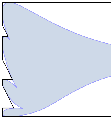
The limit shape (law of large numbers) phenomenon states that the normalized height function of a random tiling tends to a nonrandom limiting height function. The latter has a variational description (Cohn–Kenyon–Propp [CKP01] and Kenyon–Okounkov [KO07]). In many problems, in particular, for uniformly random lozenge tilings of the so-called sawtooth polygons considered in Petrov [Pet14] (see Figure 1), the variational problem can be solved in terms of algebraic equations for the gradient of the limiting height function.

In a neighborhood where the limiting height function is non-flat, the local (bulk) correlations of a random tiling should be described by an ergodic translation invariant Gibbs measure on tilings of the whole plane. The latter measure is unique for a given gradient, and its correlations are described by the incomplete beta kernel (an extension of the discrete sine kernel); see Sheffield [She05], Kenyon–Okounkov–Sheffield [KOS06]. This universal bulk behavior has been proven in full generality for uniformly random tilings by Aggarwal [Agg19], following the earlier works for the hexagon (Baik–Kriecherbauer–McLaughlin–Miller [BKMM07], Gorin [Gor08]), sawtooth polygons (Petrov [Pet14]), and a lozenge tiling model corresponding to the noncolliding Bernoulli simple random walks (Gorin–Petrov [GP19]). The curve separating the region where the height function is non-flat is referred to as the frozen boundary. For uniformly random tilings of polygons this curve is algebraic.

A $\mathfrak{q}$-deformation of uniformly random lozenge tilings is obtained by assigning probability weights proportional to $\mathfrak{q}^{\mathrm{volume}}$, where the volume is measured under the height function. This allows considering tilings of infinite domains (also sometimes called plane partitions) if the partition function is summable for $\mathfrak{q}\in(0,1)$ (we use a different font for $\mathfrak{q}$ to distinguish from the $q$-exchangeable parameter). Cerf–Kenyon [CK01] studied the $\mathfrak{q}$-weighted plane partitions and proved a limit shape result. Okounkov–Reshetikhin [OR03] found asymptotics of local correlations as $\mathfrak{q}\nearrow 1$, and introduced the incomplete beta kernel to describe them. In the subsequent work [OR07], they looked at random skew plane partitions which may have a back wall. Depending on the number of turns of the back wall, the frozen boundary may form several asymptotes extending to infinity, see [OR07, Figures 2, 15, 16] for illustrations.

Figure 1: A sawtooth polygon and frozen boundaries for the $\mathfrak{q}$-weighted lozenge tilings as $\mathfrak{q}=e^{-\upgamma/N}\to 1$, where $N\to+\infty$ is the linear size of the polygon. Here $\upgamma>0$ on the left and $\upgamma<0$ on the right. These frozen boundaries were obtained by Di Francesco–Guitter [DFG19].

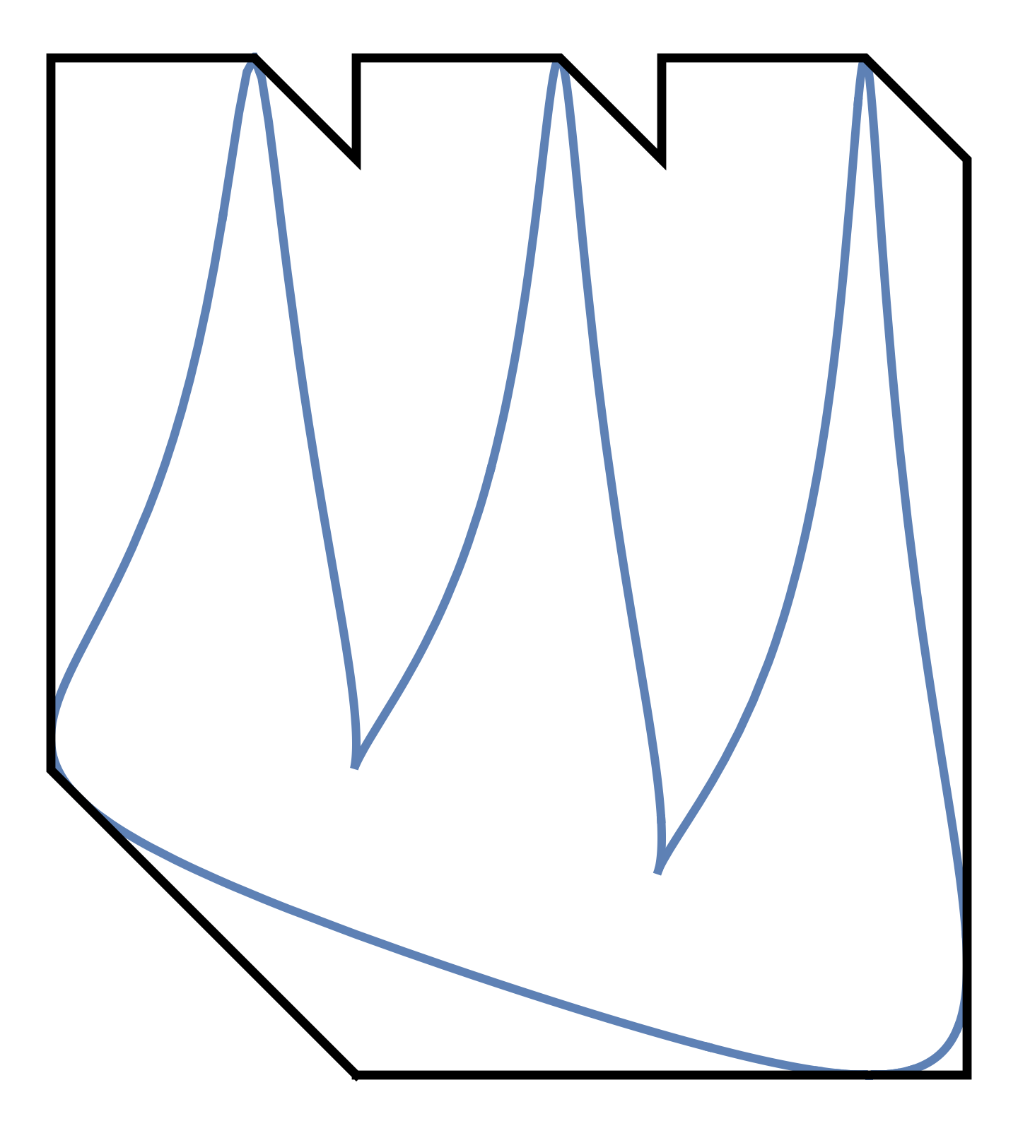
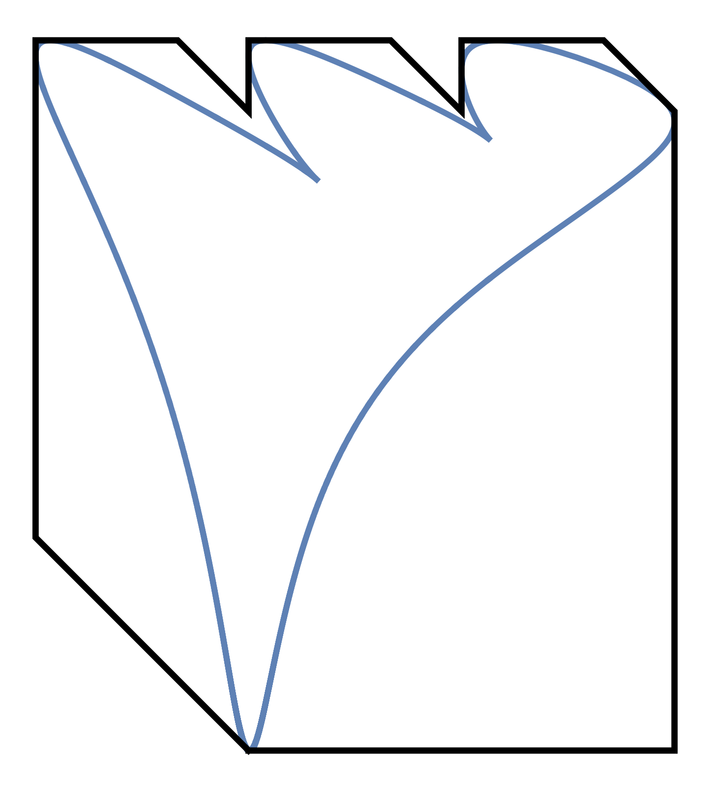
For $\mathfrak{q}$-weighted random tilings of (bounded) sawtooth polygons, the frozen boundary was computed by di Francesco–Guitter [DFG19] using the tangent method. Gorin–Huang [GH22] recently obtained it for an even more general ensemble with $(\mathfrak{q},\kappa)$-weights introduced by Borodin–Gorin–Rains [BGR10]. The boundaries of [DFG19] turn into the ones of [OR07] in a limit when the side of the sawtooth polygon with multiple defects tends to infinity. Then the “cloud” parts adjacent to this side degenerate into multiple asymptotes.

For sawtooth polygons, bulk universality of the $\mathfrak{q}$-weighted lozenge tilings as $\mathfrak{q}\to 1$ is still open except for the hexagon case settled by Borodin–Gorin–Rains [BGR10]. This is despite the explicit double contour integral expression for the correlation kernel $K_{\mathrm{loz}}$ (a close relative of the inverse Kasteleyn matrix) given by Petrov [Pet14] which we recall in (4.2) below. The reason is that the $\mathfrak{q}$-hypergeometric function under the integral in $K_{\mathrm{loz}}$ has hindered its direct asymptotic analysis.

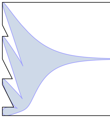
It is known that the $\mathfrak{q}$-dependent kernel $K_{\mathrm{loz}}$ (and its subsequent asymptotic analysis) simplifies in several cases. First, setting $\mathfrak{q}=1$, we get a kernel for uniformly random tilings, which has led to many asymptotic results; see Petrov [Pet14], [Pet15], Toninelli–Laslier [LT15], Gorin–Petrov [GP19], Aggarwal [Agg19]. In another regime, keeping $\mathfrak{q}<1$ fixed and sending the top boundary of the polygon (which has several turns) up to infinity, as in Figure 1, left, one can show that the $\mathfrak{q}$-weighted random tilings in a bottom part of the picture converge to the random plane partitions with a back wall studied by Okounkov–Reshetikhin [OR07]. Moreover, in this limit, the correlation kernel $K_{\mathrm{loz}}$ turns into the simpler kernel [OR07, (25)] obtained originally via the technique of Schur processes. The latter kernel is amenable to asymptotic analysis by the standard steepest descent method, which in particular leads to the frozen boundary with several asymptotes (already visible in Figure 1) and bulk universality.

Our model $\Upsilon_{m}$ of noncolliding $q$-exchangeable random walks presents a new case when the complicated kernel $K_{\mathrm{loz}}$ simplifies. Namely, if instead of $\mathfrak{q}<1$, we keep $\mathfrak{q}>1$, and send the bottom boundary of the polygon down to infinity as in Figure 1, right, then around the top boundary of the polygon we have the convergence to the noncolliding $q$-exchangeable random walks, with $q=\mathfrak{q}^{-1}$. The resulting correlation kernel $K_{\mathrm{walks}}$ has an explicit double contour integral form for any initial condition in the noncolliding walks. From this kernel, we obtain the limit shape and bulk universality results as the number $m$ of walks goes to infinity and $q=e^{-\gamma/m}\to 1$. The frozen boundary for the noncolliding walks (see Figure 3 for examples) may form several “cloud turns”, and always has exactly one asymptote (already seen forming in Figure 1, right).

We conclude that limit shape results for ensembles of random lozenge tilings are accessible by a variety of methods, but bulk universality requires knowledge or precise control of the inverse Kasteleyn matrix (or its close relative, the correlation kernel). The $q^{\mathrm{volume}}$ ensemble of random lozenge tilings of sawtooth polygons is an example of a model where such control is still out of reach. In the present paper, we explore a new degeneration of this lozenge tiling model, which is amenable to asymptotic analysis, as well as has a very nice interpretation as noncolliding $q$-exchangeable random walks with arbitrary initial conditions.

Outline

Above in the Introduction, we gave an overview of where our model $\Upsilon_{m}$ fits into the classes of noncolliding walks and random lozenge tilings. Below in Section 2 we describe our model and results in full detail. In particular, we show that our process $\Upsilon_{m}$ coincides with the system of independent $q$-exchangeable random walks conditioned never to collide. The proofs of the determinantal kernel and the asymptotic results are given in Sections 3, 4 and 5.

Acknowledgments

LP is grateful to Zhongyang Li for an initial discussion of the problem. The work was partially supported by the NSF grants DMS-1664617 and DMS-2153869, and the Simons Collaboration Grant for Mathematicians 709055. This material is based upon work supported by the National Science Foundation under grant DMS-1928930 while the first author participated in the program “Universality and Integrability in Random Matrix Theory and Interacting Particle Systems” hosted by the Mathematical Sciences Research Institute in Berkeley, California, during the Fall 2021 semester.

2 Model and main results

In this section, we discuss our model of noncolliding $q$-exchangeable random walks and formulate our main results on its determinantal structure and asymptotic behavior.

2.1 The $q$-exchangeable random walk

Consider a discrete-time simple random walk $\{y(t)\}_{t\in\mathbb{Z}_{\geq 0}}$ on $\mathbb{Z}$ making steps $0$ (“straight”) and $-1$ (“down”) according to independent flips of a given (possibly biased) coin. It is well-known that the sequence of steps in this random walk is exchangeable, that is,

$$\mathop{\mathrm{Prob}}\left(y(t+1)-y(t)=\epsilon_{1},\hskip 1.0pty(t+2)-y(t+1)=\epsilon_{2},\ldots,y(t+k)-y(t+k-1)=\epsilon_{k}\right)$$ (2.1)

is symmetric in $\epsilon_{1},\ldots,\epsilon_{k}\in\left\{0,-1\right\}$ for any $t\geq 0$ and $k\geq 1$.

Gnedin–Olshanski [GO09] considered a $q$-deformation of the concept of exchangeability depending on a parameter $q\in(0,1)$. For a $q$-exchangeable random walk $\{y(t)\}_{t\in\mathbb{Z}_{\geq 0}}$, the quantity (2.1) is no longer symmetric in $\epsilon_{1},\ldots,\epsilon_{k}$. Instead, we have the following $q$-symmetry under elementary transpositions $\epsilon_{i}\leftrightarrow\epsilon_{i+1}$:

$$\mathop{\mathrm{Prob}}\left(\ldots,y(t+i)-y(t+i-1)=\epsilon_{i},\hskip 1.0pty(t+i+1)-y(t+i)=\epsilon_{i+1},\ldots\right)\\ =q^{\epsilon_{i}-\epsilon_{i+1}}\mathop{\mathrm{Prob}}\left(\ldots,y(t+i)-y(t+i-1)=\epsilon_{i+1},\hskip 1.0pty(t+i+1)-y(t+i)=\epsilon_{i},\ldots\right).$$

In words, under a transposition of the neighboring steps $(\textnormal{down},\textnormal{straight})\to(\textnormal{straight},\textnormal{down})$, the probability of the trajectory is multiplied by $q$.

Remark 2.1.

By convention, throughout all exact computations in the paper, the parameter $q$ is a fixed number between $0$ and $1$. For the asymptotic analysis of the noncolliding $q$-exchangeable random walks, we send $q\nearrow 1$. These asymptotic results are formulated in Section 2.6 and proven in Section 5.

The space of laws (probability distributions) of $q$-exchangeable random walks is a convex simplex. That is, the convex combination (mixture) of probability laws preserves $q$-exchangeability. By a $q$-analogue of the de Finetti’s theorem proven in [GO09], extreme $q$-exchangeable random walks (that is, extreme points of this simplex) are parametrized by $\Delta\coloneqq\left\{0,1,2,\ldots\right\}\cup\left\{\infty\right\}$. In detail, for any $q$-exchangeable random walk $y(t)$, there exists a probability measure $\mu$ on $\Delta$ such that the law of $y(t)$ is a mixture of the extreme distributions by means of $\mu$.

Our first observation is that all extreme $q$-exchangeable random walks parametrized by points of $\Delta_{\mathrm{fin}}\coloneqq\left\{0,1,2,\ldots\right\}\subset\Delta$ are one and the same space-inhomogeneous random walk with varying initial configuration and an absorbing wall at $0$.

Definition 2.2 (The $q$-exchangeable random walk in $\mathbb{Z}_{\geq 0}$).

Let $\Upsilon_{1}$ be the following one-step Markov transition probability, where $x,y\in\mathbb{Z}_{\geq 0}$:

$$\Upsilon_{1}(x,y)\coloneqq\begin{cases}q^{x},&y=x;\\ 1-q^{x},&y=x-1;\\ 0,&\textnormal{otherwise}.\end{cases}$$

Proposition 2.3.

1. Started from any $x\in\mathbb{Z}_{\geq 0}$, the random walk with transition probabilities $\Upsilon_{1}$ is $q$-exchangeable.

2. Any extreme $q$-exchangeable random walk parametrized by a point $x\in\Delta_{\mathrm{fin}}$ can be identified with the random walk $\Upsilon_{1}$ started from $x$.

Proof.

For the first part, we have

$$\Upsilon_{1}(x,x)\Upsilon_{1}(x,x-1)=q^{x}(1-q^{x})=q\cdot\Upsilon_{1}(x,x-1)\Upsilon_{1}(x-1,x-1),$$

which immediately implies the $q$-exchangeability. The second part follows by comparing our random walk with the one described in [GO09, Proposition 4.1]. ∎

Remark 2.4.

In the scaling limit as $q=e^{-\varepsilon}\to 1$ and $x=\lfloor\varepsilon^{-1}\log(1/p)\rfloor+\tilde{x}$, where $p\in(0,1)$ and $\tilde{x}\in\mathbb{Z}$, the $q$-exchangeable random walk on $\mathbb{Z}_{\geq 0}$ turns into the usual simple random walk on $\mathbb{Z}$. The latter corresponds to independent coin flips with the probability of Heads equal to $p$.

2.2 Noncolliding simple random walks

The central object of the present paper is a model of several interacting $q$-exchangeable random walks which never collide. Here we first discuss the well-known model of noncolliding simple random walks on $\mathbb{Z}$. Thanks to Remark 2.4, this well-known model may be viewed as a $q\to 1$ limit of our model of noncolliding $q$-exchangeable random walks. We define the latter in detail in Section 2.3 below.

The model of noncolliding simple random walks on $\mathbb{Z}$ dates back to Karlin–McGregor [KM59]. The model of noncolliding Brownian motions on $\mathbb{R}$ is the celebrated Dyson Brownian motion for the Gaussian Unitary Ensemble [Dys62]. A systematic treatment of noncolliding random walks connecting them to determinantal point processes (in particular, orthogonal polynomial ensembles) is performed by König–O’Connell–Roch [KOR02].

The one-step Markov transition probability of a model of $m$ independent discrete-time simple random walks on $\mathbb{Z}$ (making steps $0$ and $-1$ with probabilities $p$ and $1-p$) conditioned never to collide has the form of a Doob’s $h$-transform [Doo84, 2.VI.13]

$$\Upsilon_{m}^{(q=1)}(\vec{x},\vec{y})=\frac{h_{m}^{(q=1)}(\vec{y})}{h_{m}^{(q=1)}(\vec{x})}\hskip 1.0pt\underbrace{\prod_{i=1}^{m}\big{(}p\hskip 1.0pt\mathbf{1}_{y_{i}=x_{i}}+(1-p)\hskip 1.0pt\mathbf{1}_{y_{i}=x_{i}-1}\big{)}}_{\Upsilon_{m,\mathrm{ind}}^{(q=1)}(\vec{x},\vec{y})},$$ (2.2)

where $\vec{x}=(x_{1}>\ldots>x_{m})$, $\vec{y}=(y_{1}>\ldots>y_{m})$, $x_{i},y_{i}\in\mathbb{Z}$. Here

$$h_{m}^{(q=1)}(\vec{x})\coloneqq\prod_{1\leq i<j\leq m}(x_{i}-x_{j})$$ (2.3)

is the Vandermonde determinant, and the product over $i$ in (2.2) is simply the one-step Markov transition probability of a collection of $m$ independent simple random walks, which we denoted by $\Upsilon_{m,\mathrm{ind}}^{(q=1)}$. In (2.2) and throughout the text, $\mathbf{1}_{A}$ stands for the indicator of an event or a condition $A$.

The fact that (2.2) defines a random walk of $m$ particles is not straightforward. The key property is that the right-hand side sums to $1$ over all $\vec{y}$. Equivalently, $h_{m}^{(q=1)}(\vec{x})$ is a nonnegative harmonic function for the collection of $m$ independent simple random walks:

$$\sum_{\vec{y}}h_{m}^{(q=1)}(\vec{y})\hskip 1.0pt\Upsilon_{m,\mathrm{ind}}^{(q=1)}(\vec{x},\vec{y})=h_{m}^{(q=1)}(\vec{x}).$$ (2.4)

2.3 Noncolliding $q$-exchangeable random walks

Here we describe our main model $\Upsilon_{m}$, which is a $q$-deformation of the classical model of noncolliding simple random walks from Section 2.2. For $m=1$, the model $\Upsilon_{1}$ is the $q$-exchangeable random walk from Section 2.1 above.

Denote by $\mathbb{W}_{m}$ the space of $m$-particle configurations in $\mathbb{Z}_{\geq 0}$:

$$\mathbb{W}_{m}\coloneqq\{\vec{x}=(x_{1}>x_{2}>\ldots>x_{m}\geq 0)\}\subset\mathbb{Z}_{\geq 0}^{m},$$ (2.5)

and set $|\vec{x}|\coloneqq x_{1}+\ldots+x_{m}$.

Definition 2.5.

We consider a Markov chain $\Upsilon_{m}$ on $\mathbb{W}_{m}$ with the following one-step transition probabilities, where $\vec{x},\vec{y}\in\mathbb{W}_{m}$:

$$\Upsilon_{m}(\vec{x},\vec{y})=q^{-\binom{m}{2}+(m-1)\left(|\vec{x}|-|\vec{y}|\right)}\prod_{1\leq i<j\leq m}\frac{q^{y_{j}}-q^{y_{i}}}{q^{x_{j}}-q^{x_{i}}}\underbrace{\prod_{i=1}^{m}\bigl{(}q^{x_{i}}\mathbf{1}_{y_{i}=x_{i}}+(1-q^{x_{i}})\mathbf{1}_{y_{i}=x_{i}-1}\bigr{)}}_{\Upsilon_{m,\mathrm{ind}}(\vec{x},\vec{y})}.$$ (2.6)

See Figure 2, left, for an illustration of the trajectory of the process $\Upsilon_{m}$ (with $m=4$) started from $\vec{x}=(7,6,3,1)$. As time goes to infinity, the dynamics $\Upsilon_{m}$ reaches its unique absorbing state $\delta_{m}\coloneqq(m-1,m-2,\ldots,1,0)\in\mathbb{W}_{m}$. We call the Markov process $\Upsilon_{m}$ the noncolliding $q$-exchangeable random walks.

The process $\Upsilon_{m}$ was introduced recently by Petrov [Pet22]. It is a particular $t=q$ case of the Macdonald noncolliding random walks, and the main goal of the present paper is a detailed asymptotic investigation of the $t=q$ case. It turns out that the $t=q$ process is determinantal with an explicit double contour integral kernel. The asymptotic analysis of the general $(q,t)$ Macdonald case should be performed by different, non-determinantal methods (potentially based on [GH22]), but we leave this question out of the scope of the present work.

From the results of [Pet22] it follows that for any $\vec{x}\in\mathbb{W}_{m}$, the quantities $\Upsilon_{m}(\vec{x},\vec{y})$ are nonnegative and sum to $1$ over all $\vec{y}\in\mathbb{W}_{m}$. Equivalently, the following $q$-deformation of the Vandermonde determinant

$$h_{m}(\vec{x})\coloneqq q^{-(m-1)|\vec{x}|}\prod_{1\leq i<j\leq m}(q^{x_{j}}-q^{x_{i}})$$ (2.7)

is a nonnegative eigenfunction for $\Upsilon_{m,\mathrm{ind}}$, the collection of $m$ independent $q$-exchangeable random walks:

$$\sum_{\vec{y}\in\mathbb{W}^{m}}h_{m}(\vec{y})\hskip 1.0pt\Upsilon_{m,\mathrm{ind}}(\vec{x},\vec{y})=q^{\binom{m}{2}}h_{m}(\vec{x}).$$ (2.8)

This property is similar to (2.4), but observe that here the function $h_{m}$ is not harmonic with eigenvalue $1$, but instead, its eigenvalue is equal to $q^{\binom{m}{2}}$.

From (2.6)–(2.8) we see that the transition probabilities of the dynamics $\Upsilon_{m}$ have a Doob’s $h$-transform like form. Moreover, similarly to the simple random walk case in Section 2.2, our process $\Upsilon_{m}$ can be obtained from the independent $q$-exchangeable walks $\Upsilon_{m,\mathrm{ind}}$ by conditioning them never to collide. To formulate this result (Proposition 2.6 below), we need some notation. Denote by $\Upsilon_{1}^{(T)}$ the $T$-step transition probability of the single $q$-exchangeable random walk. One can readily compute this probability assuming that $T\geq x-y$:

$$\Upsilon_{1}^{(T)}(x,y)=\mathbf{1}_{0\leq y\leq x}\hskip 1.0pt(1-q^{x})(1-q^{x-1})\ldots(1-q^{y+1})\hskip 1.0ptq^{y(T-x+y)}\hskip 1.0pt\frac{(q;q)_{T}}{(q;q)_{x-y}(q;q)_{T-x+y}}.$$ (2.9)

Indeed, $(1-q^{x})(1-q^{x-1})\ldots(1-q^{y+1})\hskip 1.0ptq^{y(T-x+y)}$ is the probability that the walk first goes all the way down from $x$ to $y$ and then stays at $y$, and the $q$-binomial coefficient $\frac{(q;q)_{T}}{(q;q)_{x-y}(q;q)_{T-x+y}}$ comes from the $q$-exchangeability.

By [KM59], the $T$-step transition probability of an $m$-particle independent $q$-exchangeable random walk $\Upsilon_{m,\mathrm{ind}}$ conditioned on the event that the particles do not collide over these $T$ steps is equal to $\det[\Upsilon_{1}^{(T)}(x_{i},y_{j})]_{i,j=1}^{m}$, where $\vec{x},\vec{y}\in\mathbb{W}_{m}$. Therefore, the one-step transition probability from $\vec{x}$ to $\vec{y}$ of $\Upsilon_{m,\mathrm{ind}}$ conditioned to not collide up to time $T$ and to get absorbed at $\delta_{m}$ has the form

$$\frac{\det[\Upsilon_{1}^{(T-1)}(y_{i},m-j)]_{i,j=1}^{m}}{\det[\Upsilon_{1}^{(T)}(x_{i},m-j)]_{i,j=1}^{m}}\hskip 1.0pt\Upsilon_{m,\mathrm{ind}}(\vec{x},\vec{y})\hskip 1.0pt\mathbf{1}_{y_{i}-x_{i}\in\left\{0,-1\right\}\textnormal{ for all $i$}}.$$

Proposition 2.6.

For any $\vec{x},\vec{y}\in\mathbb{W}_{m}$, we have

$$\lim_{T\to+\infty}\frac{\det[\Upsilon_{1}^{(T-1)}(y_{i},m-j)]_{i,j=1}^{m}}{\det[\Upsilon_{1}^{(T)}(x_{i},m-j)]_{i,j=1}^{m}}=q^{-\binom{m}{2}+(m-1)\left(|\vec{x}|-|\vec{y}|\right)}\prod_{1\leq i<j\leq m}\frac{q^{y_{j}}-q^{y_{i}}}{q^{x_{j}}-q^{x_{i}}}.$$ (2.10)

Proof.

Using (2.9) and factoring out $q^{\sum_{j=1}^{m}(m-j)(T-1+m-j)}$ and $q^{\sum_{j=1}^{m}(m-j)(T+m-j)}$, respectively, from the numerator and the denominator in the right-hand side (2.10) yields the factor $q^{-\binom{m}{2}}$ in the left-hand side. After this, we can pass to the limit as $T\to\infty$ in the matrix elements of each determinant because the resulting matrices stay nondegenerate. Thus, it remains to compute one such determinant with $T=\infty$, say (after replacing the index $j$ with $m+1-j$):

$$\det\Bigl{[}\mathbf{1}_{0\leq j-1\leq x_{i}}\hskip 1.0pt\frac{(1-q^{x_{i}})(1-q^{x_{i}-1})\ldots(1-q^{j})\hskip 1.0ptq^{-x_{i}(j-1)}}{(q;q)_{x_{i}-j+1}}\Bigr{]}_{i,j=1}^{m}=\det\Bigl{[}\frac{q^{-x_{i}(j-1)}(q^{x_{i}-j+2};q)_{j-1}}{(q;q)_{j-1}}\Bigr{]}_{i,j=1}^{m}.$$ (2.11)

Here we rewrote the products in a convenient form, and observed that the indicator $\mathbf{1}_{0\leq j-1\leq x_{i}}$ is automatically enforced in the right-hand side by the $q$-Pochhammer $(q^{x_{i}-m+j+1};q)_{j-1}$.

We see that each $(i,j)$-th entry in the determinant in the right-hand side of (2.11) is a polynomial in $q^{-x_{i}}$ of degree $j-1$. Therefore, the whole determinant is proportional to the Vandermonde $\prod_{1\leq i<j\leq m}(q^{x_{j}}-q^{x_{i}})$. One readily sees that the coefficient by this Vandermonde is equal to $\frac{(-1)^{m(m-1)/2}q^{-(m-1)|\vec{x}|}}{(q;q)_{1}(q;q)_{2}\ldots(q;q)_{m-1}}$, which completes the proof. ∎

The limit relation in Proposition 2.6 completes the analogy between the well-known model of noncolliding simple random walks on $\mathbb{Z}$ (and the Dyson Brownian motion) and our noncolliding $q$-exchangeable random walks $\Upsilon_{m}$. In both cases, the $h$-transform structure of the transition probability is due to the conditioning that the independent random walks never collide.

2.4 Gibbs interpretation as $q$-weighted lozenge tilings

The $m$-particle process $\Upsilon_{m}$ satisfies a version of the $q$-exchangeability discussed for a single random walk in Section 2.1. Namely, this is the Gibbs property of the walk observed in [Pet22].

Fix $m$ and an initial condition $\vec{x}\in\mathbb{W}_{m}$ for the process $\Upsilon_{m}$. Under a suitable affine transformation of the trajectory of $\Upsilon_{m}$, it can be bijectively identified with a lozenge tiling of the vertical strip of width $x_{1}+1$, see Figure 2, right. The bottom boundary of the vertical strip is encoded by $\vec{x}$ in the following way. Viewing $\vec{x}$ as a particle configuration in $\mathbb{Z}_{\geq 0}$, each particle $x_{i}$ corresponds to a straight piece in the boundary of slope $(-1/\sqrt{3})$, and each hole in $\vec{x}$ corresponds to cutting a small triangle out of the strip. Due to the eventual absorption of the walk $\Upsilon_{m}$ at $\delta_{m}$, the lozenge tiling is “frozen” far at the top, with $x_{1}+1-m$ tiles of one type on the left followed by $m$ tiles of the other type. Thus, each lozenge tiling corresponding to a trajectory of $\Upsilon_{m}$ contains only finitely many horizontal lozenges.

Figure 2: Left: Illustration of the trajectory of the noncolliding $q$-exchangeable random walks $\Upsilon_{m}$ (with $m=4$) started from $\vec{x}=(7,6,3,1)$. Right: A bijective interpretation of the trajectory as a lozenge tiling of a strip via an affine transformation.

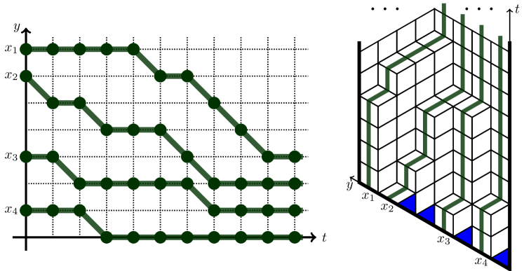
The lozenge tiling corresponding to a trajectory of $\Upsilon_{m}$ can be interpreted as a stepped surface in three dimensions such that the solid under this surface is made out of $1\times 1\times 1$ boxes. Via this interpretation, each trajectory of $\Upsilon_{m}$ has a well-defined volume under the corresponding stepped surface. In other words, the volume of a given tiling is the number of boxes which must be added to the minimal configuration to get this tiling. For example, the volume of the tiling in Figure 2, right, is equal to 34.

The next statement follows from [Pet22, Proposition 10].

Proposition 2.7.

Fix $m$ and $\vec{x}\in\mathbb{W}_{m}$. The probability distribution of the trajectory of the Markov process $\Upsilon_{m}$ (2.6) started from $\vec{x}$ is the same as the distribution of the random lozenge tiling of the strip as in Figure 2, right (depending on $\vec{x}$), where the probability weight of a tiling is proportional to $q^{\mathrm{volume}}$.

Remark 2.8.

Another $q$-dependent model of noncolliding random walks was introduced and studied in [BG13]. In that model, the parameter $q$ enters the particle speeds $1,q^{-1},q^{-2},\ldots$, but the dynamics as a whole satisfies the usual, undeformed exchangeability property. Indeed, the single-particle dynamics in [BG13] is the simple random walk (with Poisson, Bernoulli, or geometric jumps), and our single-particle dynamics is the $q$-exchangeable random walk.

Let us denote the $q^{\mathrm{volume}}$-weighted probability measure on tilings described in Proposition 2.7 by $\mathscr{M}_{m}^{(\vec{x})}$. The partition function (that is, the probability normalizing constant) of $\mathscr{M}_{m}^{(\vec{x})}$ has an explicit form:

Proposition 2.9.

The sum of the quantities $q^{\mathrm{volume}}$ over all lozenge tilings of the strip as in Figure 2, right (determined by $\vec{x}\in\mathbb{W}_{m}$), is equal to

$$Z[\mathscr{M}_{m}^{(\vec{x})}]=\prod_{i=1}^{m}\frac{1}{(q;q)_{x_{i}}}\prod_{1\leq i<j\leq m}(1-q^{x_{i}-x_{j}}).$$ (2.12)

Note in particular that setting $q=0$, we get $Z[\mathscr{M}_{m}^{(\vec{x})}]=1$, as it should be.

Proof of Proposition 2.9.

From Proposition 2.7, it suffices to check that $1/Z[\mathscr{M}_{m}^{(\vec{x})}]$ is the transition probability (over $x_{1}-m+1$ steps) of fastest path from $\vec{x}$ to the absorbing state $\delta_{m}$. This fact follows by taking the product of the one-step transition probabilities (2.6) and observing that the $q$-Vandermonde factors cancel out, except for the first such factor coming from the initial condition $\vec{x}$. The resulting expression for $1/Z[\mathscr{M}_{m}^{(\vec{x})}]$ is then verified directly. ∎

2.5 Determinantal kernel

Fix $m\in\mathbb{Z}_{\geq 1}$ and an initial configuration $\vec{x}\in\mathbb{W}_{m}$ for the noncolliding $q$-exchangeable random walks $\Upsilon_{m}$ (Definition 2.5). View the trajectory $\vec{y}(t)$ of the process $\Upsilon_{m}$ as a random point configuration $\{y_{j}(t)\colon j=1,\ldots,m,\,t\in\mathbb{Z}_{\geq 0}\}\subset\mathbb{Z}^{2}_{\geq 0}$. The next statement is our first main result.

Theorem 2.10.

Thus defined random point configuration in $\mathbb{Z}_{\geq 0}^{2}$ forms a determinantal point process, that is, for any $\ell\geq 1$ and any pairwise distinct points $(u_{i},t_{i})\in\mathbb{Z}_{\geq 0}^{2}$, we have

$$\begin{split}&\mathrm{Prob}\left(\textnormal{the random configuration $\{y_{j}(t)\colon 1\leq j\leq m,\,t\geq 0\}$ contains all $(u_{i},t_{i})$, $i=1,\ldots,\ell$}\right)\\ &\hskip 280.0pt=\det\bigl{[}K_{\mathrm{walks}}(u_{i},t_{i};u_{j},t_{j})\bigr{]}_{i,j=1}^{\ell},\end{split}$$ (2.13)

where the correlation kernel $K_{\mathrm{walks}}$ has double contour integral form:

$$\begin{split}&K_{\mathrm{walks}}(y_{1},t_{1};y_{2},t_{2})\coloneqq\mathbf{1}_{t_{1}=t_{2}}\mathbf{1}_{y_{1}=y_{2}}-\mathbf{1}_{t_{2}>t_{1}}\mathbf{1}_{y_{2}+t_{2}>y_{1}+t_{1}}\frac{q^{(t_{1}-t_{2})(y_{1}+t_{1})}(q^{y_{1}-y_{2}+t_{1}-t_{2}+1};q)_{t_{2}-t_{1}-1}}{(q;q)_{t_{2}-t_{1}-1}}\\ &\hskip 20.0pt-\frac{q^{-t_{1}-y_{1}}}{(2\pi\mathbf{i})^{2}}\oiint dz\hskip 1.0ptdw\hskip 1.0pt\frac{z^{-t_{2}}w^{t_{1}}}{w-z}\frac{(q;q)_{t_{1}}}{(wq^{-y_{1}-t_{1}};q)_{t_{1}+1}}\frac{(zq^{1-y_{2}-t_{2}};q)_{t_{2}-1}}{(q;q)_{t_{2}-1}}\frac{(w^{-1};q)_{\infty}}{(z^{-1};q)_{\infty}}\prod_{r=1}^{m}\frac{1-q^{x_{r}}/z}{1-q^{x_{r}}/w}.\end{split}$$ (2.14)

Here $y_{1},y_{2}\in\mathbb{Z}$, $t_{1}\in\mathbb{Z}_{\geq 0}$, $t_{2}\in\mathbb{Z}_{>0}$, the $w$ contour is an arbitrarily small circle around $0$, and the $z$ contour goes around $q^{y_{2}+t_{2}},q^{y_{2}+t_{2}+1},q^{y_{2}+t_{2}+2},\ldots$, $0$, the $w$ contour, and encircles no other $z$ poles of the integrand.

We prove Theorem 2.10 in Section 4 below after relating (in Section 3) the process $\Upsilon_{m}$ of noncolliding $q$-exchangeable random walks to a $q$-weighted distribution on lozenge tilings of a sawtooth polygons. The determinantal kernel for the latter is known from [Pet14].

2.6 Asymptotic results

Recall the definition of a determinantal kernel which should appear in the bulk of our noncolliding $q$-exchangeable random walks as the number of walks and the time go to infinity:

Definition 2.11.

Let $\omega\in\mathbb{C}\setminus\{0,1\}$, $\mathop{\mathrm{Im}}\omega\geq 0$, be a parameter called the complex slope. The incomplete beta kernel is defined as

$$\mathsf{B}_{\omega}(\Delta t,\Delta p):=\frac{1}{2\pi\i}\int_{\overline{\omega}}^{\omega}(1-u)^{\Delta t}u^{-\Delta p-1}du,\qquad\Delta t,\Delta p\in\mathbb{Z},$$ (2.15)

where the integration arc from $\overline{\omega}$ to $\omega$ crosses $(0,1)$ for $\Delta t\geq 0$ and $(-\infty,0)$ for $\Delta t<0$.

The kernel (2.15) was introduced in [OR03] to describe local asymptotics of a certain ensemble of $q$-distributed random lozenge tilings of the whole plane (equivalent to random plane partitions). Moreover, the incomplete beta kernel is the universal bulk scaling limit of uniformly random lozenge tilings of bounded shapes [Agg19]. By [She05], [KOS06], for every complex slope $\omega$, there is a unique ergodic translation invariant Gibbs measure on lozenge tilings of the whole plane, and its determinantal correlation kernel is $\mathsf{B}_{\omega}$.

Let us now describe the asymptotic regime of our random walks. Let $m\to+\infty$, and set $q=e^{-\gamma/m}$ for fixed $\gamma>0$. Scale the time and the space variables in the random walk (as in Figure 2, left) proportionally to $m$: $t=\lfloor\tau m\rfloor$, $y=\lfloor\rho m\rfloor$, where $\tau,\rho\in\mathbb{R}_{\geq 0}$ are fixed. Let the initial condition $\vec{x}\in\mathbb{W}_{m}$ form a fixed number $L\geq 1$ of densely packed clusters:

$$x_{i}=i+\lfloor m\hskip 1.0ptC_{k}\rfloor\quad\textnormal{for $m\hskip 1.0pta_{k}\leq i<m\hskip 1.0pta_{k+1}$},$$ (2.16)

where $i=1,\ldots,m$, $k=1,\ldots,L$, and $0<C_{1}<C_{2}<\ldots<C_{L}$ and $0=a_{1}<a_{2}<\ldots<a_{L+1}=1$ are the fixed parameters of the clusters. See the beginning of Section 5.1 for more detail.

In the $(\tau,\rho)$ plane, let $\partial\mathcal{D}$ be the curve with the following rational parametrization in the exponential coordinates $(e^{\gamma\tau},e^{\gamma\rho})$:

$$e^{\gamma\tau(w)}=\frac{(wF(w))^{\prime}-e^{-\gamma}}{wF^{\prime}(w)-F(w)+e^{\gamma}F^{2}(w)},\qquad e^{\gamma\rho(w)}=\frac{e^{\gamma}F^{\prime}(w)}{e^{\gamma}(wF(w))^{\prime}-1},\qquad w\in\mathbb{R},$$

where

$$F(w)\coloneqq\frac{w}{w-1}\prod_{i=1}^{L}\frac{w\hskip 1.0pte^{\gamma(a_{i}+C_{i})}-1}{w\hskip 1.0pte^{\gamma(a_{i+1}+C_{i})}-1}.$$

This curve bounds a domain denoted by $\mathcal{D}$ such that $\mathcal{D}\cap([0,\tau]\times\mathbb{R}_{\geq 0})$ is bounded for any $\tau>0$. We call $\partial\mathcal{D}$ the frozen boundary curve, and $\mathcal{D}$ the liquid region. See Figure 3 for examples.

Figure 3: Examples of the liquid region and the frozen boundary in the $(\tau,\rho)$ plane, with $\gamma=1/3,1$, and $3$, and the same initial conditions $\vec{a}=(0,0.1,0.2,0.6,1)$, $\vec{C}=(0.05,0.45,0.8,1)$. The bounding polygonal region indicates where the walks trajectories may lie, with the vertical straight pieces being the initial densely packed clusters of particles $\vec{x}$. Outside the liquid region, there are either no walks, or the walks are densely packed and move deterministically straight, horizontally or diagonally.

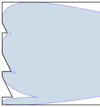
For any $(\tau,\rho)\in\mathcal{D}$, let $\omega=\omega(\tau,\rho)$ be the unique root of the algebraic equation

$$\omega\hskip 1.0ptF\Bigl{(}e^{-\gamma\rho}\hskip 1.0pt\frac{1-\omega}{1-e^{\gamma\tau}\omega}\Bigr{)}=e^{-\gamma(\tau+1)}$$

in the upper half complex plane. The existence and uniqueness of the complex root of this equation (equivalent to (5.9)) follow from Section 5.2 and the change of variables (5.19). With all this notation in place, we can now formulate the main asymptotic result of the paper:

Theorem 2.12.

For any $(\tau,\rho)\in\mathcal{D}$, in the limit regime described above, we have

$$\lim_{m\to+\infty}(-1)^{\Delta t}e^{\gamma(\tau+\rho)\Delta t}K_{\mathrm{walks}}\left(\lfloor\rho m\rfloor+\Delta p,\lfloor\tau m\rfloor+\Delta t;\lfloor\rho m\rfloor,\lfloor\tau m\rfloor\right)=\mathbf{1}_{\Delta t=\Delta p=0}-\mathsf{B}_{\omega}(\Delta t,\Delta p)$$

for any fixed $\Delta t,\Delta p\in\mathbb{Z}$.

Let us make two remarks about Theorem 2.12. First, the factor $(-1)^{\Delta t}e^{\gamma(\tau+\rho)\Delta t}$ in front of $K_{\mathrm{walks}}$ is a so-called “gauge transformation” of the correlation kernel which does not change the determinants in (2.13), and thus preserves the determinantal process. Therefore, Theorem 2.12 states that the point process of the random walks converges locally (at the lattice level, in a neighborhood of the global position $(\tau,\rho)$) to the complement of the point process coming from the unique ergodic translation invariant Gibbs measure on lozenge tilings of the whole plane with parameter $\omega$. The complement arises by the Kerov’s complementation principle (see, for example, [BOO00, Appendix A.3]) because our correlation kernel is $\mathbf{1}-\mathsf{B}_{\omega}$, where $\mathbf{1}$ is the identity operator.

Second, let us discuss the densely packed clusters assumption (2.16). On the one hand, it restricts the generality of the initial conditions. On the other hand, it leads to elegant formulas for the global frozen boundary, and simplifies the technical part of the analysis. The bulk limit asymptotics of Theorem 2.12 should follow for general initial data $\vec{x}$ by a more delicate steepest descent analysis of our kernel, similarly to what is done in [GP19] for the $q=1$ noncolliding random walks with general initial data. We do not pursue this analysis here. See also [DM15], [DM20] for limit shape and fluctuation results on uniformly random lozenge tilings with more general boundary conditions.

Finally, we make a conjecture about the final absorbing time of the noncolliding $q$-exchangeable random walks:

Remark 2.13 (Asymptotics of the absorption time of $\Upsilon_{m}$).

Note that the liquid region is unbounded. More precisely, the frozen boundary has an asymptote approaching $\rho=1$ as $\tau\to+\infty$. This implies that the absorption time of the Markov chain $\Upsilon_{m}$, that is, the random time

$$t_{\mathrm{abs}}(m)\coloneqq\min\left\{t\in\mathbb{Z}_{\geq 0}\colon y_{1}(t)=m-1\right\},$$

grows faster than $m$. Based on the result of Mutafchiev [Mut06] on unrestricted random plane partitions, we conjecture that $t_{\mathrm{abs}}(m)\sim m\log m$ as $m\to+\infty$.

It should be possible to obtain a more precise behavior with the generating function coefficients technique as in [Mut06] (based on Hayman’s admissible functions [Hay56]). Indeed, this is because our ensemble of plane partitions coming from $\Upsilon_{m}$ has an explicit partition function (Proposition 2.9).

3 From lozenge tilings to noncolliding $q$-exchangeable walks

Here we recall the result from [Pet22] which shows how the noncolliding $q$-exchangeable random walks $\Upsilon_{m}$ arise as a limit of the $q$-distributed random lozenge tilings.

3.1 $q$-distributed lozenge tilings of sawtooth polygons

Let $\mathbb{GT}_{N}$ be the set of all partitions of length $N$, that is, $N$-tuples of nonnegative integers $\lambda=(\lambda_{1}\geq\lambda_{2}\geq\dots\lambda_{N}\geq 0)$. Denote $|\lambda|=\lambda_{1}+\ldots+\lambda_{N}$. We say that $\mu\in\mathbb{GT}_{N-1}$ interlaces with $\lambda\in\mathbb{GT}_{N}$, denoted by $\mu\prec\lambda$, if $\lambda_{1}\geq\mu_{1}\geq\lambda_{2}\geq\ldots\geq\lambda_{N-1}\geq\mu_{N-1}\geq\lambda_{N}$. For a sequence

$$\Lambda=(\varnothing\prec\Lambda^{(1)}\prec\Lambda^{(2)}\prec\dots\prec\Lambda^{(N-1)}\prec\Lambda^{(N)}),\qquad\Lambda^{(j)}\in\mathbb{GT}_{j},$$ (3.1)

define its volume by

$$\mathop{\mathrm{volume}}(\Lambda)=\sum_{m=1}^{N-1}|\Lambda^{(m)}|.$$

Fix $\lambda\in\mathbb{GT}_{N}$, and consider the probability measure on sequences (3.1) with fixed top row $\Lambda^{(N)}=\lambda$, and probability weight proportional to $q^{-\mathrm{volume}(\Lambda)}$. Denote this probability measure by $\mathscr{T}_{N}^{(\lambda)}$. We may express the partition function of $\mathscr{T}_{N}^{(\lambda)}$ as follows (see, e.g., [Pet14, Section 3] for more detail):

$$Z[\mathscr{T}_{N}^{(\lambda)}]=\sum_{\Lambda\colon\Lambda^{(N)}=\lambda}q^{-\mathrm{volume}(\Lambda)}=s_{\lambda}(q^{1-N},q^{2-N},\dots,q^{-1},1),$$ (3.2)

where $s_{\lambda}$ is the Schur symmetric polynomial $s_{\lambda}(z_{1},\ldots,z_{N})=\det[z_{i}^{\lambda_{j}+N-j}]_{i,j=1}^{N}\prod\limits_{1\leq i<j\leq N}(z_{i}-z_{j})^{-1}$. The right-hand side of (3.2) may also be simplified to the product form:

$$Z[\mathscr{T}_{N}^{(\lambda)}]=q^{|\lambda|(1-N)}\prod_{1\leq i<j\leq N}\frac{q^{\lambda_{i}-i}-q^{\lambda_{j}-j}}{q^{-i}-q^{-j}}.$$

The probability measure $\mathscr{T}_{N}^{(\lambda)}$ has a bijective interpretation as a distribution on lozenge tilings of a sawtooth polygon of depth $N$ and fixed top boundary determined by $\lambda$. Define

$$p_{i}^{n}=\Lambda^{(n)}_{i}-i,\qquad 1\leq i\leq n\leq N.$$ (3.3)

Under $\mathscr{T}_{N}^{(\lambda)}$, the quantities $p_{i}^{n}$ form a random integer array $\mathfrak{P}=\{p_{i}^{n}\}_{1\leq i\leq n\leq N}$ satisfying the interlacing constraints:

$$p_{i+1}^{n}<p_{i}^{n-1}\leq p_{i}^{n}$$

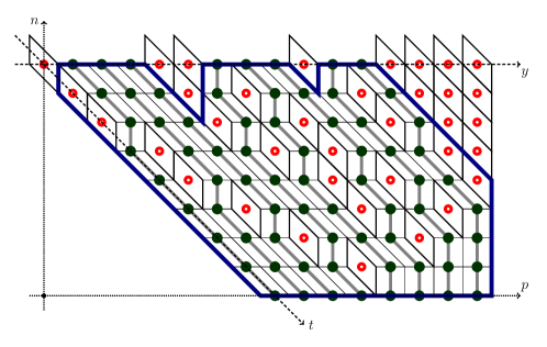
(for all $i$’s and $n$’s for which these inequalities can be written out). Viewing each $p_{i}^{n}$ as the coordinate of the center of a vertical lozenge  , we may complete the tiling in a unique way by the other two types of lozenges. This leads to a corresponding tiling of a sawtooth polygon as in Figure 4.

Figure 4: An example of a lozenge tiling of a sawtooth polygon of height $N=8$ with top row $\lambda=(16,16,16,16,14,11,11,8)$. The particle array $\mathfrak{P}=\{p^{n}_{i}\}$ consists of the red circle dots placed at the centers of the vertical lozenges, with coordinates relative to the $(p,n)$ coordinate system (with dotted axes).

Remark 3.1.

Note that the measure $\mathscr{T}_{N}^{(\lambda)}$ on lozenge tilings of a sawtooth polygon with weights proportional to $q^{-\mathrm{volume}}$ is different from the measure $\mathscr{M}_{m}^{(\vec{x})}$ described in Section 2.4 above. In particular, the tilings under $\mathscr{M}_{m}^{(\vec{x})}$ live in an infinite domain, and are weighted proportionally to $q^{+\mathrm{volume}}$. In the next Section 3.2 we explain how the measures $\mathscr{T}_{N}^{(\lambda)}$ as $N\to+\infty$ and special choice of $\lambda$ lead to $\mathscr{M}_{m}^{(\vec{x})}$.

3.2 Limit transition to random walks

Now let us connect the probability measure $\mathscr{T}_{N}^{(\lambda)}$ to the noncolliding $q$-exchangeable random walks $\Upsilon_{m}$ from Definition 2.5. Observe that for $\lambda\in\mathbb{GT}_{N}$, we have:

$$\mathscr{T}_{N}^{(\lambda)}\bigl{(}\Lambda^{(N-1)}=\mu\bigr{)}=\frac{q^{-|\mu|}\hskip 1.0ptZ[\mathscr{T}_{N-1}^{(\mu)}]}{Z[\mathscr{T}_{N}^{(\lambda)}]}=q^{(N-1)\left(|\lambda|-|\mu|\right)}\frac{s_{\mu}(1,q,\ldots,q^{N-2})}{s_{\lambda}(1,q,\ldots,q^{N-2},q^{N-1})}.$$

Indeed, the first equality follows from the $q^{-\mathrm{volume}}$ probability weights, and the second equality is due to (3.2) and the homogeneity of the Schur polynomials.

Fix $m\geq 1$ and $\vec{x},\vec{y}\in\mathbb{W}_{m}$. Let $\lambda\in\mathbb{GT}_{N}$ and $\mu\in\mathbb{GT}_{N-1}$ depend on $\vec{x},\vec{y}$ as follows (here and below we assume that $N$ is sufficiently large):

$$\begin{split}\left\{\lambda_{1}-1,\lambda_{2}-2,\ldots,\lambda_{N}-N\right\}&=\{0,1,2,\ldots,N+m-1\}\setminus\left\{x_{1},\ldots,x_{m}\right\},\\ \left\{\mu_{1}-1,\mu_{2}-2,\ldots,\mu_{N-1}-(N-1)\right\}&=\{1,2,\ldots,N+m-1\}\setminus\left\{y_{1}+1,\ldots,y_{m}+1\right\}.\end{split}$$ (3.4)

This choice of $\lambda$ and $\mu$ means that we pass from a lozenge tiling to nonintersecting paths avoiding the lozenges of type  , see Figure 4. Moreover, we choose the boundary conditions such that the number $m$ of paths stays fixed as $N$ grows.

The following result is a particular case of [Pet22, Section 3] with $t=q$:

Proposition 3.2.

With the above notation, for fixed $m$ and $\vec{x},\vec{y}\in\mathbb{W}_{m}$, we have

$$\lim_{N\to+\infty}\mathscr{T}_{N}^{(\lambda)}\bigl{(}\Lambda^{(N-1)}=\mu\bigr{)}=\Upsilon_{m}(\vec{x},\vec{y}),$$

where $\Upsilon_{m}$ is given by (2.6).

Proposition 3.2 states that the limiting distribution of the nonintersecting paths in Figure 4 is the same as the distribution of the trajectory of the noncolliding $q$-exchangeable random walks $\Upsilon_{m}$. In Figure 4, the noncolliding paths live in the coordinate system $(y,t)$ (with dashed axes), and converge $\Upsilon_{m}$ in an arbitrary finite neighborhood of the point $y=t=0$. In Section 4 below we use this limiting relation to write down the correlation kernel for the random walks $\Upsilon_{m}$.

4 Limit transition in the kernel

4.1 Correlation kernel for $q$-distributed lozenge tilings of sawtooth polygons

We begin by recalling Theorem 4.1 from [Pet14] about the correlation kernel of the measure $\mathscr{T}_{N}^{(\lambda)}$ on lozenge tilings of the sawtooth polygon with top row $\lambda$ described in Section 3.1 above. By the results of [Ken97] (see also [Bor11, Section 7]), this measure is a determinantal point process in the sense that for any $\ell\geq 1$ and any pairwise distinct $(p_{1},n_{1}),\ldots,(p_{\ell},n_{\ell})\in\mathbb{Z}^{2}$ we have

$$\mathop{\mathrm{Prob}}\left(\textnormal{the random array $\mathfrak{P}$ contains all $(p_{1},n_{1}),\ldots,(p_{\ell},n_{\ell})$}\right)=\det\left[K_{\mathrm{loz}}(p_{i},n_{i};p_{j},n_{j})\right]_{i,j=1}^{\ell}.$$ (4.1)

The kernel $K_{\mathrm{loz}}$ is computed in [Pet14, Theorem 4.1] and is given by the following double contour integral formula:

$$\begin{split}&K_{\mathrm{loz}}(p_{1},n_{1};p_{2},n_{2})=-\mathbf{1}_{n_{2}<n_{1}}\mathbf{1}_{p_{2}\leq p_{1}}q^{n_{2}(p_{1}-p_{2})}\frac{(q^{p_{1}-p_{2}+1};q)_{n_{1}-n_{2}-1}}{(q;q)_{n_{1}-n_{2}-1}}\\ &\hskip 10.0pt+\frac{(q^{N-1};q^{-1})_{N-n_{1}}}{(2\pi\mathbf{i})^{2}}\oiint\frac{dz\hskip 1.0ptdw}{w}\frac{q^{n_{2}(p_{1}-p_{2})}z^{n_{2}}}{w-z}\\ &\hskip 20.0pt\times{}_{2}\phi_{1}(q^{-1},q^{n_{1}-1};q^{N-1}\mid q^{-1};w^{-1})\hskip 1.0pt\frac{(zq^{1-p_{2}+p_{1}};q)_{N-n_{2}-1}}{(q;q)_{N-n_{2}-1}}\prod_{r=1}^{N}\frac{w-q^{\lambda_{r}-r-p_{1}}}{z-q^{\lambda_{r}-r-p_{1}}}.\end{split}$$ (4.2)

Here the points $(p_{1},n_{1}),(p_{2},n_{2})\in\mathbb{Z}^{2}$ are such that $1\leq n_{1}\leq N$, $1\leq n_{2}\leq N-1$. The $z$ and $w$ integration contours are counterclockwise and do not intersect. The $z$ contour encircles $q^{p_{2}-p_{1}},q^{p_{2}-p_{1}+1},\ldots,q^{\lambda_{1}-1-p_{1}}$ and not $q^{p_{2}-p_{1}-1},q^{p_{2}-p_{1}-2},\ldots$. The $w$ contour is sufficiently large and goes around $0$ and the $z$ contour. Finally, ${}_{2}\phi_{1}$ in (4.2) is the (in this case, terminating) Gauss $q$-hypergeometric function given by

$${}_{2}\phi_{1}(q^{-1},q^{n_{1}-1};q^{N-1}\mid q^{-1};w^{-1})=\sum_{j=0}^{n_{1}-1}\frac{(q^{-1};q^{-1})_{j}(q^{n_{1}-1};q^{-1})_{j}}{(q^{N-1};q^{-1})_{j}}\frac{w^{-j}}{(q^{-1};q^{-1})_{j}}.$$ (4.3)

In the rest of this section we consider the $N\to+\infty$ limit of the kernel $K_{\mathrm{loz}}$ in the regime leading to the noncolliding $q$-exchangeable random walks (as discussed in Section 3.2), and prove Theorem 2.10.

4.2 Rewriting the kernel

Fix $t_{1}\geq 0$, $t_{2}>0$, and let $n_{1}=N-t_{1},n_{2}=N-t_{2}$ (throughout the rest of the section we assume that $N$ is sufficiently large). Change the integration variables in (4.2) as $\tilde{z}=zq^{p_{1}}$, $\tilde{w}=wq^{p_{1}}$, and then rename back to $z,w$. We have

$$\begin{split}&q^{N(p_{2}-p_{1})}K_{\mathrm{loz}}(p_{1},N-t_{1};p_{2},N-t_{2})=-\mathbf{1}_{t_{2}>t_{1}}\mathbf{1}_{p_{2}\leq p_{1}}q^{(-t_{2})(p_{1}-p_{2})}\frac{(q^{p_{1}-p_{2}+1};q)_{t_{2}-t_{1}-1}}{(q;q)_{t_{2}-t_{1}-1}}\\ &\hskip 10.0pt+\frac{(q^{N-1};q^{-1})_{t_{1}}}{(2\pi\mathbf{i})^{2}}\oiint\frac{dz\hskip 1.0ptdw}{w}\frac{q^{(-t_{2})(p_{1}-p_{2})}z^{N-t_{2}}q^{-p_{1}(N-t_{2})}}{w-z}\\ &\hskip 20.0pt\times{}_{2}\phi_{1}(q^{-1},q^{N-t_{1}-1};q^{N-1}\mid q^{-1};w^{-1}q^{p_{1}})\frac{(zq^{1-p_{2}};q)_{t_{2}-1}}{(q;q)_{t_{2}-1}}\prod_{r=1}^{N}\frac{w-q^{\lambda_{r}-r}}{z-q^{\lambda_{r}-r}}.\end{split}$$ (4.4)

Here the $z$ contour encircles only $q^{p_{2}},q^{p_{2}+1},q^{p_{2}+2},\ldots$ and no other $z$ poles of the integrand, and the $w$ contour goes around $0$ and the $z$ contour.

The factor $q^{N(p_{2}-p_{1})}$ is a so-called “gauge transformation” of the correlation kernel which does not change the determinants in (4.1) and thus preserves the determinantal process. In general, by a gauge transformation we mean replacing a kernel $K(p_{1},t_{1};p_{2},t_{2})$ by $\frac{f(p_{1},t_{1})}{f(p_{2},t_{2})}K(p_{1},t_{1};p_{2},t_{2})$, where $f$ is nowhere vanishing.

In the next step, we use the fact that the top row $\lambda$ depends on $N$ as in (3.4). Here $\vec{x}\in\mathbb{W}_{m}$ is the fixed initial configuration of the noncolliding $q$-exchangeable random walks $\Upsilon_{m}$. Relation (3.4) allows to express the last product over $r$ in the integrand in (LABEL:eq:K_rewrite_1) in terms of the $x_{j}$’s. After necessary simplifications, we obtain

$$\begin{split}&q^{N(p_{2}-p_{1})}K_{\mathrm{loz}}(p_{1},N-t_{1};p_{2},N-t_{2})=-\mathbf{1}_{t_{2}>t_{1}}\mathbf{1}_{p_{2}\leq p_{1}}q^{(-t_{2})(p_{1}-p_{2})}\frac{(q^{p_{1}-p_{2}+1};q)_{t_{2}-t_{1}-1}}{(q;q)_{t_{2}-t_{1}-1}}\\ &\hskip 10.0pt+\frac{(q^{N-1};q^{-1})_{t_{1}}}{(2\pi\mathbf{i})^{2}}\oiint\frac{dz\hskip 1.0ptdw}{w}\frac{z^{-t_{2}}q^{p_{2}t_{2}}}{w-z}q^{-Np_{1}}w^{N}{}_{2}\phi_{1}(q^{-1},q^{N-t_{1}-1};q^{N-1}\mid q^{-1};w^{-1}q^{p_{1}})\\ &\hskip 20.0pt\times\frac{(zq^{1-p_{2}};q)_{t_{2}-1}}{(q;q)_{t_{2}-1}}\prod_{j=0}^{N+m-1}\frac{1-q^{j}/w}{1-q^{j}/z}\prod_{r=1}^{m}\frac{1-q^{x_{r}}/z}{1-q^{x_{r}}/w}.\end{split}$$ (4.5)

The integration contours in (4.5) are the same as in (LABEL:eq:K_rewrite_1).

4.3 Exchanging the contours

We now move the $w$ contour inside the $z$ contour in (4.5). The integral stays the same, but we need to add a contour integral of minus the residue $\mathop{\mathrm{Res}}_{z=w}$ over the $w$ contour around $0$. The residue is equal to

$$\begin{split}&-\mathop{\mathrm{Res}}\nolimits_{z=w}=\frac{(q^{N-1};q^{-1})_{t_{1}}}{2\pi\mathbf{i}}\frac{1}{w}w^{-t_{2}}q^{p_{2}t_{2}}\\ &\hskip 80.0pt\times q^{-Np_{1}}w^{N}{}_{2}\phi_{1}(q^{-1},q^{N-t_{1}-1};q^{N-1}\mid q^{-1};w^{-1}q^{p_{1}})\frac{(wq^{1-p_{2}};q)_{t_{2}-1}}{(q;q)_{t_{2}-1}}.\end{split}$$ (4.6)

Lemma 4.1.

The integral in $w$ of (4.6) over a small contour around zero is equal to

$$\mathbf{1}_{t_{2}>t_{1}}q^{(-t_{2})(p_{1}-p_{2})}\frac{(q^{p_{1}-p_{2}+1};q)_{t_{2}-t_{1}-1}}{(q;q)_{t_{2}-t_{1}-1}}.$$

Proof.

Notice that ${}_{2}\phi_{1}(q^{-1},q^{N-t_{1}-1};q^{N-1}\mid q^{-1};w^{-1}q^{p_{1}})$ and $(wq^{1-p_{2}};q)_{t_{2}-1}$ are Laurent polynomials in $w$. Therefore, the integral of (4.6) over a small contour around zero is simply the operation of picking the coefficient by $1/w$.

By the $q$-binomial theorem, we can write

$$\begin{split}(wq^{1-p_{2}};q)_{t_{2}-1}&=(w^{-1}q^{p_{2}-t_{2}+1};q)_{t_{2}-1}(-wq^{1-p_{2}})^{t_{2}-1}q^{\binom{t_{2}-1}{2}}\\ &=(-wq^{1-p_{2}})^{t_{2}-1}q^{\binom{t_{2}-1}{2}}\sum_{j=0}^{t_{2}-1}(-1)^{j}q^{(p_{2}-t_{2}+1)j}q^{\binom{j}{2}}\frac{(q;q)_{t_{2}-1}}{(q;q)_{j}(q;q)_{t_{2}-1-j}}w^{-j}.\end{split}$$ (4.7)

Using formula (4.3) for ${}_{2}\phi_{1}$ and (4.7), the product of the two Laurent polynomials has the form

$$\sum_{j=0}^{N-t_{1}-1}q^{p_{1}j}\frac{(q^{N-t_{1}-1};q^{-1})_{j}}{(q^{N-1};q^{-1})_{j}}w^{-j}\times\sum_{j=0}^{t_{2}-1}(-1)^{j}q^{(p_{2}-t_{2}+1)j}q^{\binom{j}{2}}\frac{(q;q)_{t_{2}-1}}{(q;q)_{j}(q;q)_{t_{2}-1-j}}w^{-j}=\sum_{j=0}^{N+t_{2}-t_{1}-2}\mathsf{d}_{j}w^{-j}.$$

From the prefactor in (4.6) we see that we need to compute the sum $\mathsf{d}_{N-1}$ which has the form

$$\mathsf{d}_{N-1}=\sum_{m=0}^{N-1}q^{p_{1}(N-1-m)}q^{\binom{m}{2}}(-1)^{m}q^{(p_{2}-t_{2}+1)m}\frac{(q^{N-t_{1}-1};q^{-1})_{N-1-m}}{(q^{N-1};q^{-1})_{N-1-m}}\frac{(q;q)_{t_{2}-1}}{(q;q)_{m}(q;q)_{t_{2}-1-m}}.$$

Observe that $m$-th term in the sum vanishes for $m>t_{2}$ or $m<t_{1}$, so the limits of the summation are $\mathbf{1}_{t_{2}>t_{1}}\sum_{m=t_{1}}^{t_{2}-1}$. Rearranging the terms and relabeling $k=m-t_{1}$, we have

$$\begin{split}\mathsf{d}_{N-1}&=\mathbf{1}_{t_{2}>t_{1}}(-1)^{t_{1}}\frac{(q^{t_{2}-t_{1}},q)_{t_{1}}}{(q^{N-t_{1}},q)_{t_{1}}}q^{p_{1}(N-1-t_{1})+\binom{t_{1}}{2}+(p_{2}-t_{2}+1)t_{1}}\\ &\hskip 90.0pt\times\sum_{k=0}^{t_{2}-t_{1}-1}q^{(t_{1}-p_{1}+p_{2}-t_{2}+1)k}q^{\binom{k}{2}}(-1)^{k}\frac{(q;q)_{t_{2}-t_{1}-1}}{(q;q)_{k}(q;q)_{t_{2}-t_{1}-1-k}}.\end{split}$$

Applying the $q$-binomial theorem, we can simplify this sum to:

$$\mathsf{d}_{N-1}=\mathbf{1}_{t_{2}>t_{1}}(-1)^{t_{1}}\frac{(q^{t_{2}-t_{1}};q)_{t_{1}}}{(q^{N-t_{1}},q)_{t_{1}}}q^{p_{1}(N-1-t_{1})+\binom{t}{2}+(p_{2}-t_{2}+1)t_{1}}(q^{t_{1}-p_{1}+p_{2}-t_{2}+1};q)_{t_{2}-t_{1}-1}.$$

Putting together all factors from the above computation completes the proof. ∎

By Lemma 4.1, the kernel takes the form

$$\begin{split}&q^{N(p_{2}-p_{1})}K_{\mathrm{loz}}(p_{1},N-t_{1};p_{2},N-t_{2})=\mathbf{1}_{t_{2}>t_{1}}\mathbf{1}_{p_{2}>p_{1}}q^{(-t_{2})(p_{1}-p_{2})}\frac{(q^{p_{1}-p_{2}+1};q)_{t_{2}-t_{1}-1}}{(q;q)_{t_{2}-t_{1}-1}}\\ &\hskip 10.0pt+\frac{(q^{N-1};q^{-1})_{t_{1}}}{(2\pi\mathbf{i})^{2}}\oiint\frac{dz\hskip 1.0ptdw}{w}\frac{z^{-t_{2}}q^{p_{2}t_{2}}}{w-z}\hskip 1.0ptq^{-Np_{1}}w^{N}{}_{2}\phi_{1}(q^{-1},q^{N-t_{1}-1};q^{N-1}\mid q^{-1};w^{-1}q^{p_{1}})\\ &\hskip 20.0pt\times\frac{(zq^{1-p_{2}};q)_{t_{2}-1}}{(q;q)_{t_{2}-1}}\prod_{j=0}^{N+m-1}\frac{1-q^{j}/w}{1-q^{j}/z}\prod_{r=1}^{m}\frac{1-q^{x_{r}}/z}{1-q^{x_{r}}/w}.\end{split}$$ (4.8)

The integration contours in (4.8) have changed, namely, the $w$ contour is an arbitrarily small circle around $0$, and the $z$ contour goes around $q^{p_{2}},q^{p_{2}+1},q^{p_{2}+2},\ldots$, $0$, the $w$ contour, and encircles no other $z$ poles of the integrand. In (4.8), the first summand is a combination of the residue from Lemma 4.1 and the first summand in the previous expression (4.5).

4.4 Limit of the $q$-hypergeometric function

After exchanging the $z$ and $w$ contours, $|w|$ can be taken arbitrarily small. This allows to take a limit in $N$ in the part of the integrand in (4.8) containing the $q$-hypergeometric function ${}_{2}\phi_{1}$ (observe that this is essentially the only dependence on $N$ left in the integrand). Denote

$$Q_{N}(w)\coloneqq(q^{N-1};q^{-1})_{t_{1}}q^{-Np_{1}}w^{N}{}_{2}\phi_{1}(q^{-1},q^{N-t_{1}-1};q^{N-1}\mid q^{-1};w^{-1}q^{p_{1}}).$$

Then

$$\begin{split}Q_{N}(w)&=(q^{N-1};q^{-1})_{t_{1}}q^{-Np_{1}}w^{N}\sum_{j=0}^{N-t_{1}-1}\frac{(q^{N-t_{1}-1};q^{-1})_{j}}{(q^{N-1};q^{-1})_{j}}\hskip 1.0ptw^{-j}q^{jp_{1}}\\ &=(q^{N-1};q^{-1})_{t_{1}}\sum_{k=0}^{N-t_{1}-1}\frac{(q^{N-t_{1}-1};q^{-1})_{N-t_{1}-1-k}}{(q^{N-1};q^{-1})_{N-t_{1}-1-k}}(w/q^{p_{1}})^{t_{1}+1+k},\end{split}$$

where we used (4.3) and in the last line flipped the summation index as $k=N-t_{1}-1-j$. We have

$$\lim_{N\to+\infty}(q^{N-1};q^{-1})_{t_{1}}=1.$$

Next, in each $k$-th term in the sum we have (for $k$ fixed):

$$\frac{(q^{N-t_{1}-1};q^{-1})_{N-t_{1}-1-k}}{(q^{N-1};q^{-1})_{N-t_{1}-1-k}}\hskip 1.0pt(w/q^{p_{1}})^{t_{1}+1+k}\\ =(w/q^{p_{1}})^{t_{1}+1+k}\prod_{i=0}^{N-t_{1}-k-2}\frac{1-q^{k+i+1}}{1-q^{t_{1}+k+i+1}}\to(w/q^{p_{1}})^{t_{1}+1+k}\prod_{i=0}^{t_{1}-1}(1-q^{k+i+1}),\qquad N\to+\infty,$$

and because $|w|$ is small, the convergence is uniform in $k$ and $w$. Thus, we have

$$\lim_{N\to+\infty}Q_{N}(w)=\sum_{k=0}^{\infty}(w/q^{p_{1}})^{t_{1}+1+k}(q^{k+1};q)_{t_{1}},$$ (4.9)

uniformly in $w$ for small $|w|$.

Lemma 4.2.

The sum in the right-hand side of (4.9) is equal to

$$(w/q^{p_{1}})^{t_{1}+1}\frac{(q;q)_{t_{1}}}{(wq^{-p_{1}};q)_{t_{1}+1}}.$$

Proof.

We have

$$\begin{split}\sum_{k=0}^{\infty}(wq^{-p_{1}})^{t_{1}+1+k}(q^{k+1},q)_{t_{1}}&=(wq^{-p_{1}})^{t_{1}+1}(q;q)_{t_{1}}\sum_{k=0}^{\infty}(wq^{-p_{1}})^{k}\frac{(q,q)_{k+t_{1}}}{(q;q)_{k}(q;q)_{t_{1}}}\\ &=(wq^{-p_{1}})^{t_{1}+1}\frac{(q;q)_{t_{1}}}{(wq^{-p_{1}};q)_{t_{1}+1}},\end{split}$$

where we used the $q$-binomial theorem, and the series converges because $|w|$ is small. ∎

Putting together the formula (4.8) for the kernel $K_{\mathrm{loz}}$ and the results of the current Section 4.4, we arrive at a $N\to+\infty$ limit of the kernel $K_{\mathrm{loz}}$. Denote

$$\begin{split}K_{\mathrm{loz}}^{\mathrm{lim}}(p_{1},t_{1};p_{2},t_{2})&\coloneqq\mathbf{1}_{t_{2}>t_{1}}\mathbf{1}_{p_{2}>p_{1}}\frac{q^{-t_{2}(p_{1}-p_{2})}(q^{p_{1}-p_{2}+1};q)_{t_{2}-t_{1}-1}}{(q;q)_{t_{2}-t_{1}-1}}+\frac{q^{p_{2}t_{2}-p_{1}t_{1}-p_{1}}}{(2\pi\mathbf{i})^{2}}\oiint dz\hskip 1.0ptdw\hskip 1.0pt\frac{z^{-t_{2}}w^{t_{1}}}{w-z}\\ &\hskip 65.0pt\times\frac{(q;q)_{t_{1}}}{(wq^{-p_{1}};q)_{t_{1}+1}}\frac{(zq^{1-p_{2}};q)_{t_{2}-1}}{(q;q)_{t_{2}-1}}\frac{(w^{-1};q)_{\infty}}{(z^{-1};q)_{\infty}}\prod_{r=1}^{m}\frac{1-q^{x_{r}}/z}{1-q^{x_{r}}/w},\end{split}$$ (4.10)

where the $w$ contour is an arbitrarily small circle around $0$, and the $z$ contour goes around $q^{p_{2}},q^{p_{2}+1},q^{p_{2}+2},\ldots$, $0$, the $w$ contour, and encircles no other $z$ poles of the integrand.

The next proposition follows directly from the previous computations.

Proposition 4.3.

For any fixed $t_{1}\geq 0$, $t_{2}>0$, $p_{1},p_{2}\in\mathbb{Z}$, we have

$$\lim_{N\to+\infty}q^{N(p_{2}-p_{1})}K_{\mathrm{loz}}(p_{1},N-t_{1};p_{2},N-t_{2})=K_{\mathrm{loz}}^{\mathrm{lim}}(p_{1},t_{1};p_{2},t_{2}).$$

4.5 Particle-hole involution and time shift

We are now in a position to derive Theorem 2.10 from the limit transition of Proposition 4.3. Define

$$K_{\mathrm{walks}}(y_{1},t_{1};y_{2},t_{2})\coloneqq\mathbf{1}_{t_{1}=t_{2}}\mathbf{1}_{y_{1}=y_{2}}-q^{t_{1}(t_{1}+y_{1})-t_{2}(t_{2}+y_{2})}K_{\mathrm{loz}}^{\mathrm{lim}}(y_{1}+t_{1},t_{1};y_{2}+t_{2},t_{2}).$$ (4.11)

Observe that we performed two transformations to get $K_{\mathrm{walks}}$ from $K_{\mathrm{loz}}^{\mathrm{lim}}$ in (4.11):

1. First, the point process defined by the noncolliding walks (formed by the solid dots in Figure 4) is the complement of the process defined by the particles $p^{n}_{i}$. Therefore, by the Kerov’s complementation principle (see, for example, [BOO00, Appendix A.3]), the kernel for the walks is the identity minus the kernel for the lozenges.

2. Second, the shifting of the variables $p_{i}=y_{i}+t_{i}$, $i=1,2$, corresponds to the passage from the coordinate system $(p,n)$ (where $n=N-t$) to the coordinate system $(y,t)$, see Figure 4.

Finally, the factor in front of $K_{\mathrm{loz}}^{\mathrm{lim}}$ in (4.11) is simply a gauge transformation which does not change the determinantal process. One can readily verify that the resulting kernel $K_{\mathrm{walks}}$ (4.11) is the same as (2.14). This completes the proof of Theorem 2.10.

5 Asymptotic analysis

In this section, we perform the bulk asymptotic analysis of the correlation kernel $K_{\mathrm{walks}}$ (2.14) of the process $\Upsilon_{m}$ in the regime as $q\to 1$, $m\to\infty$, and the initial configuration $\vec{x}$ forms a finite number of densely packed clusters. We make the latter assumption for technical convenience, see, e.g., Duse–Metcalfe [DM15], [DM20] for asymptotic results on uniformly random lozenge tilings with more general boundaries. Using the steepest descent method, we prove Theorem 2.12, that is, obtain the limit shape of the trajectories of $\Upsilon_{m}$, as well as the universal local fluctuations of the paths which are governed by the incomplete beta kernel introduced by Okounkov–Reshetikhin [OR03]. The latter is a two-dimensional extension of the discrete sine kernel introduced by Borodin–Okounkov–Olshanski [BOO00].

5.1 Limit regime

The limit regime we consider for the kernel $K_{\mathrm{walks}}(p_{1},t_{1};p_{2},t_{2})$ (2.14) is as follows:

$$m\to+\infty;\qquad q=e^{-\gamma/m}\nearrow 1;\qquad t_{2}=\lfloor m\tau\rfloor,\quad t_{1}=t_{2}+\Delta t;\qquad p_{2}=\lfloor m\rho\rfloor,\quad p_{1}=p_{2}+\Delta p.$$ (5.1)

Here $(\tau,\rho)\in\mathbb{R}^{2}_{\geq 0}$, $\gamma>0$, and the quantities $\Delta t=t_{1}-t_{2},\Delta p=p_{1}-p_{2}\in\mathbb{Z}$ are fixed. The regime with fixed differences $\Delta t,\Delta p$ is called bulk limit, and it describes local correlations around the global point of observation $(\tau,\rho)\in\mathbb{R}^{2}_{\geq 0}$. Finally, we assume that the initial configuration $\vec{x}\in\mathbb{W}_{m}$ scales as follows:

$$x_{i}=\lfloor m\hskip 1.0ptg\left(i/m\right)\rfloor,\quad 1\leq i\leq m;\qquad g(u)=\sum_{i=1}^{L}(u+C_{i})\mathbf{1}_{u\in[a_{i},a_{i+1})},$$ (5.2)

where $L\geq 1$ is fixed (this is the number of clusters of densely packed particles in $\vec{x}$), and

$$0<C_{1}<C_{2}<\ldots<C_{L},\qquad 0=a_{1}<a_{2}<\ldots<a_{L+1}=1$$ (5.3)

are the parameters of the clusters, and $g(u)$ is weakly increasing with derivative $0$ or $1$.

We apply the standard steepest descent approach outlined in [Oko02, Section 3]. For this, we first rewrite the integrand in the double integral in $K_{\mathrm{walks}}(p_{1},t_{1};p_{2},t_{2})$ (2.14) as

$$\begin{split}&-\frac{q^{-t_{1}-p_{1}}}{(2\pi\mathbf{i})^{2}}\frac{z^{-t_{2}}w^{t_{1}}}{w-z}\frac{(q;q)_{t_{1}}}{(wq^{-p_{1}-t_{1}};q)_{t_{1}+1}}\frac{(zq^{1-p_{2}-t_{2}};q)_{t_{2}-1}}{(q;q)_{t_{2}-1}}\frac{(w^{-1};q)_{\infty}}{(z^{-1};q)_{\infty}}\prod_{r=1}^{m}\frac{1-q^{x_{r}}/z}{1-q^{x_{r}}/w}\\ &\hskip 2.0pt=-\frac{q^{-t_{1}-p_{1}}}{(2\pi\mathbf{i})^{2}}\frac{(q;q)_{t_{1}}}{(q;q)_{t_{2}-1}}\frac{1}{(w-z)(1-zq^{-p_{2}})(1-zq^{-p_{2}-t_{2}})}\hskip 1.0pt\exp\left\{m\left(S_{m}(w;t_{1},p_{1})-S_{m}(z;t_{2},p_{2})\right)\right\},\end{split}$$

where

$$\begin{split}S_{m}(w;t,p)&\coloneqq\frac{t}{m}\log w-\frac{1}{m}\sum_{i=0}^{t}\log(1-wq^{-p-t+i})\\ &\hskip 90.0pt+\frac{1}{m}\sum_{i=0}^{\infty}\log(1-w^{-1}q^{i})-\frac{1}{m}\sum_{r=1}^{m}\log(1-w^{-1}q^{x_{r}}).\end{split}$$ (5.4)

Here we can take any branches of the logarithms so that $S_{m}$ is holomorphic in $w$ belonging to the upper half complex plane. Indeed, any branches taken the same in $S_{m}(w;t_{1},p_{1})$ and $S_{m}(z;t_{2},p_{2})$ produce the same signs in the exponent in the integrand.

Using (5.1)–(5.2), let us define the limiting version of the function $S_{m}$:

$$\begin{split}S(w;\tau,\rho)&\coloneqq\tau\log w-\int_{0}^{\tau}\log\left(1-we^{\gamma(\tau+\rho-u)}\right)du\\ &\hskip 90.0pt+\int_{0}^{\infty}\log\left(1-w^{-1}e^{-\gamma u}\right)du-\int_{0}^{1}\log\left(1-w^{-1}e^{-\gamma g(u)}\right)du.\end{split}$$ (5.5)

Lemma 5.1.

We have $S_{m}(w;\lfloor m\tau\rfloor,\lfloor m\rho\rfloor)=S(w;\tau,\rho)+O(m^{-1})$ as $m\to+\infty$, uniformly for $w$ and $(\tau,\rho)$ belonging to compact subsets of $\left\{w\colon\mathop{\mathrm{Im}}w>0\right\}$ and $\mathbb{R}_{\geq 0}^{2}$, respectively.

Proof.

This follows from the convergence of the Riemann sums in (5.4) to the corresponding integrals in (5.5), as the integrands are piecewise $C^{1}$ functions in $u$ with norms uniformly bounded in $w,\tau,\rho$ belonging to compact subsets of their respective domains. ∎

Integrals in (5.5) can be expressed through the dilogarithm function which has the series and the integral representations

$$\mathrm{Li}_{2}(\xi)=\sum_{k=1}^{\infty}\frac{\xi^{k}}{k^{2}}=-\eta\int_{0}^{\infty}\log\left(1-\xi e^{-\eta u}\right)du.$$ (5.6)

The series converges for $|\xi|<1$, and the integral representation (valid for any $\eta>0$, but we will mostly use it with $\eta=\gamma$) follows a certain branch of the logarithm. For example, we may choose a branch of $\mathrm{Li}_{2}(\xi)$ to have cut at $\xi\in\mathbb{R}_{\geq 1}$. We have

$$\mathrm{Li}_{2}^{\prime}(\xi)=-\frac{\log(1-\xi)}{\xi},\qquad\frac{\partial}{\partial\xi}\hskip 1.0pt\xi\hskip 1.0pt\frac{\partial}{\partial\xi}\hskip 1.0pt\mathrm{Li}_{2}(\xi)=\frac{1}{1-\xi}.$$ (5.7)

With this notation and using (5.2), we have

$$\begin{split}S(w;\tau,\rho)&=\tau\log w-\gamma^{-1}\mathrm{Li}_{2}(we^{\gamma\rho})+\gamma^{-1}\mathrm{Li}_{2}\bigl{(}we^{\gamma(\rho+\tau)}\bigr{)}\\ &\hskip 30.0pt-\gamma^{-1}\mathrm{Li}_{2}(w^{-1})+\gamma^{-1}\sum_{i=1}^{L}\left[\mathrm{Li}_{2}\bigl{(}w^{-1}e^{-\gamma(a_{i}+C_{i})}\bigr{)}-\mathrm{Li}_{2}\bigl{(}w^{-1}e^{-\gamma(a_{i+1}+C_{i})}\bigr{)}\right].\end{split}$$ (5.8)

5.2 Critical points and the frozen boundary

Let us count the critical points of $S(w;\tau,\rho)$ in the complex upper half-plane. Recall that $w$ is a critical point if, by definition, $S^{\prime}(w;\tau,\rho)=0$, where the derivative is taken in $w$. By looking at $e^{\gamma wS^{\prime}(w;\tau,\rho)}$, we see that the critical points must satisfy the following algebraic equation:

$$\frac{w\hskip 1.0pte^{\gamma(\tau+1)}}{w-1}\cdot\frac{we^{\gamma\rho}-1}{we^{\gamma(\rho+\tau)}-1}\prod_{i=1}^{L}\frac{w\hskip 1.0pte^{\gamma(a_{i}+C_{i})}-1}{w\hskip 1.0pte^{\gamma(a_{i+1}+C_{i})}-1}=1.$$ (5.9)

Lemma 5.2.

For any $\tau,\rho>0$, equation (5.9) has at most one non-real root in $w$ in the complex upper half-plane.

We denote this root in the upper half-plane by $w_{c}=w_{c}(\tau,\rho)$.

Proof of Lemma 5.2.

Denote by $p_{num}(w)$ and $p_{den}(w)$ the polynomials in the denominator and the numerator, respectively, in the left-hand side of (5.9). Let us first count the real roots of (5.9) by considering intersections of the graphs of $p_{num}(w)$ and $p_{den}(w)$, $w\in\mathbb{R}$. Both polynomials $p_{num}$ and $p_{den}$ are of degree $L+2$, and have only real roots. Since their top degree coefficients have the same sign, we may and will assume that $p_{num}(-\infty)=p_{den}(-\infty)=+\infty$.

The roots of $p_{num}(w)$ are $0$, $e^{-\gamma\rho}$, and $w^{num}_{i}\coloneqq e^{-\gamma(a_{i}+C_{i})}$, $1\leq i\leq L$. Similarly, $p_{den}(w)$ has roots $1,e^{-\gamma(\rho+\tau)}$, and $w^{den}_{i}\coloneqq e^{-\gamma(a_{i+1}+C_{i})}$, $1\leq i\leq L$. By (5.2), the roots interlace as

$$0\leq w_{den}^{i}<w_{num}^{i}<w_{den}^{i-1}\leq 1,\qquad 2\leq i\leq L.$$ (5.10)

We first discuss two examples illustrating how we count the roots. Let us start with $\rho>(a_{L+1}+C_{L})$. Then the two leftmost roots of $p_{den}(w)$ are $0$ and $e^{-\rho}$, and the two leftmost roots of $p_{num}(w)$ are $e^{-\gamma(\rho+\tau)}$ and $e^{-\gamma(a_{L+1}+C_{L})}$. Moreover, $0<e^{-\gamma(\rho+\tau)}<e^{-\rho}<e^{-\gamma(a_{L+1}+C_{L})}$. We see that on each of $L+1$ segments between the roots of $p_{num}$, the graph of $p_{num}$ intersects with the graph of $p_{den}$. This counting produces at least $L+1$ real solutions to (5.9). Since this equation is equivalent to a polynomial equation of degree at most $L+2$, it follows that there are no complex solutions to (5.9). See Figure 5 for an illustration.

Figure 5: Graphs of $p_{num}$ and $p_{den}$ for large $\rho$.

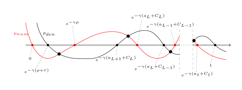
Let us now decrease $\rho$ while keeping $\rho+\tau$ constant. At some point we will have a repeated root $e^{-\gamma\rho}=e^{-\gamma(a_{L+1}+C_{L})}$, which upon further decreasing $\rho$ breaks the interlacing. Then we can have $L-1$ or $L+1$ roots (counted with multiplicity) at the intersections of the graphs of $p_{num}$ and $p_{den}$, see Figure 6 for an illustration. When there are $L-1$ intersections, (5.9) may have a single pair of complex conjugate non-real roots. We see that there cannot be more than one such pair.

Now let us describe what happens for $\rho<(a_{L+1}+C_{L})$. Recall that $e^{-\gamma(a_{L+1}+C_{L})}\leq e^{-\gamma\rho}\leq 1$, so for some $1\leq i\leq L$ we have $w^{den}_{i}\leq e^{-\gamma\rho}\leq w^{den}_{i-1}$, where we set $w^{den}_{0}=1$ for convenience. From $\eqref{eq:L_interlacing_roots}$ we also have $w^{den}_{i}<w^{num}_{i}<w^{den}_{i-1}$, thus we have two roots of the numerator, namely $w^{num}_{i}$ and $e^{-\gamma\rho}$ located between two roots of denominator. Denote the interval between $w^{num}_{i}$ and $e^{-\gamma\rho}$ by $I$, so $[0,1]=[0,\min(w^{num}_{i},e^{-\gamma\rho})]\cup I\cup[\max(w^{num}_{i},e^{-\gamma\rho}),1]$. Note that some of these intervals might be empty in the presence of double roots of $p_{num}$.

If $e^{-\gamma(\rho+\tau)}\in I$, then the interlacing is restored, and we have a structure similar to the first case as in Figure 5. The graphs of $p_{num}$ and $p_{den}$ intersect $L+1$ times, which gives at least $L+1$ real critical points, and thus no complex roots exist.

Figure 6: Graphs of $p_{num}$ and $p_{den}$ for $\rho+\tau>a_{L+1}+c_{L}>\rho>a_{L}+c_{L}$. Possible dashed graphs lead to nonexistence of complex roots, and solid graphs lead to exactly one complex root in the upper half-plane.

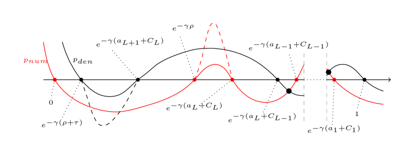
On the other hand, if $e^{-\gamma(\rho+\tau)}\notin I$, the configuration is similar to Figure 6, and we have either $L-1$ or $L+1$ intersections, leaving the possibility that at most one complex root in the upper half-plane exists. This completes the proof. ∎

Definition 5.3.

Let $\mathcal{D}\subset\mathcal{P}$ be the open set of pairs $(\tau,\rho)$, such that $S(w;\tau,\rho)$ defined by (5.5), (5.8) has one non-real critical point $w_{c}$ in the upper half-plane. We call $\mathcal{D}$ liquid region, and its boundary curve $\partial\mathcal{D}$ the frozen boundary.

Let us obtain a parametrization of the frozen boundary $\partial\mathcal{D}$. Because the equation (5.9) has real coefficients, as $(\tau,\rho)$ approaches $\partial\mathcal{D}$, the corresponding critical point $w_{c}$ becomes close with its complex conjugate $\overline{w}_{c}$. At $\partial\mathcal{D}$ these two roots of (5.9) merge, and thus the frozen boundary is the discriminant curve of the equation (5.9). We may thus take $w_{c}\in\mathbb{R}$ as a parameter of this curve $\tau=\tau(w_{c})$, $\rho=\rho(w_{c})$.

Denote

$$F(w)\coloneqq\frac{w}{w-1}\prod_{i=1}^{L}\frac{w\hskip 1.0pte^{\gamma(a_{i}+C_{i})}-1}{w\hskip 1.0pte^{\gamma(a_{i+1}+C_{i})}-1}.$$

Then the two equations for the double roots of (5.9) yield a rational parametrization of $\partial\mathcal{D}$ in the exponential coordinates $(e^{\gamma\tau},e^{\gamma\rho})$:

$$e^{\gamma\tau(w)}=\frac{(wF(w))^{\prime}-e^{-\gamma}}{wF^{\prime}(w)-F(w)+e^{\gamma}F^{2}(w)},\qquad e^{\gamma\rho(w)}=\frac{e^{\gamma}F^{\prime}(w)}{e^{\gamma}(wF(w))^{\prime}-1},\qquad w\in\mathbb{R}.$$ (5.11)

We used this explicit parametrization to draw the frozen boundaries in Figure 3 from Section 2.6.

5.3 Analysis of $S(w;\tau,\rho)$

In this subsection we assume that $(\tau,\rho)\in\mathcal{D}$, and investigate the behavior of the steepest descent contours $\mathop{\mathrm{Im}}S(w;\tau,\rho)=\mathop{\mathrm{Im}}S(w_{c};\tau,\rho)$ started from the critical point $w_{c}$. In the next Section 5.4 we use this information to deform the original integration contours in $K_{\mathrm{walks}}$ (2.14) to the steepest descent ones. This will yield Theorem 2.12.

First, we consider the behavior of $\mathop{\mathrm{Im}}S(w;\tau,\rho)$ close to the real line, that is, $w=v+\mathbf{i}\varepsilon$, $v\in\mathbb{R}$, and $\varepsilon>0$ is sufficiently small and fixed. In $\log w$ and $\mathrm{Li}_{2}(w)$ entering (5.8) we choose the standard branch of the logarithm which has branch cut along the negative real line. Using the integral representation in (5.6), we see that $\mathrm{Li}_{2}(\xi)$ has branch cut along $[1,+\infty)$.

Lemma 5.4.

For sufficiently small fixed $\varepsilon>0$, the graph of the function $v\mapsto\mathop{\mathrm{Im}}S(v+\mathbf{i}\varepsilon;\tau,\rho)$, $v\in\mathbb{R}$, has at most four intersections with any horizontal line. If there are four intersections, then the leftmost of these intersections is in a small left neighborhood of zero, and goes to $0$ as $\varepsilon\to 0$.

See Figure 7 for an illustration of the graph of this function.

Proof of Lemma 5.4.

Observe the following behavior of the functions entering (5.8):

1. The graph of

   $$v\mapsto\mathop{\mathrm{Im}}(\tau\log(v+\mathbf{i}\varepsilon))=\tau\tan^{-1}(\varepsilon/v)+\pi\tau\mathbf{1}_{v<0}$$

   is in an $O(\varepsilon)$ neighborhood of the graph of the step function $v\mapsto\pi\tau\mathbf{1}_{v<0}$ with the added vertical segment from $(0,\pi)$ to $(0,0)$.

2. The graph of $v\mapsto\mathop{\mathrm{Im}}\bigl{(}\mathrm{Li}_{2}(v+\mathbf{i}\varepsilon)\bigr{)}$ is in an $O(\varepsilon)$ neighborhood of the graph of the function $\chi_{+}(v)\coloneqq\pi\log v\cdot\mathbf{1}_{v>1}$. Indeed, this is because

   $$\begin{split}\mathop{\mathrm{Im}}\bigl{(}\mathrm{Li}_{2}(v+\mathbf{i}\varepsilon)\bigr{)}&=-\int_{0}^{\infty}\mathop{\mathrm{Arg}}\left(1-(v+\mathbf{i}\varepsilon)e^{-u}\right)du\\ &=\pi\int_{0}^{\infty}\mathbf{1}_{1-ve^{-u}<0}\hskip 1.0ptdu+O(\varepsilon)\\ &=\pi\log v\cdot\mathbf{1}_{v>1}+O(\varepsilon).\end{split}$$ (5.12)

3. The graph of $v\mapsto\mathop{\mathrm{Im}}\bigl{(}\mathrm{Li}_{2}\left(1/(v+\mathbf{i}\varepsilon)\right)\bigr{)}$ is in an $O(\varepsilon)$ neighborhood of the graph of the function $\chi_{-}(v)\coloneqq\pi\log v\cdot\mathbf{1}_{0<v<1}$ with the added vertical line from $(0,0)$ to $(0,-\infty)$. This fact is obtained similarly to the expansion (5.12).

Figure 7: The graph of $v\mapsto\mathop{\mathrm{Im}}S(v+\mathbf{i}\varepsilon;\tau,\rho)$ for small $\varepsilon$. For any fixed $\varepsilon>0$ this function is continuous. Its maximum is in the neighborhood of zero and has order $O(\left|\log\varepsilon\right|)$.

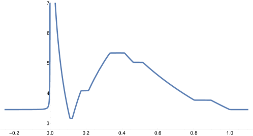
Thus, for small $\varepsilon$ the graph of $v\mapsto\mathop{\mathrm{Im}}S(v+\mathbf{i}\varepsilon;\tau,\rho)$ belongs to an $O(\varepsilon)$ neighborhood of the graph of the following function:

$$\begin{split}&S_{\mathbb{R}}(v;\tau,\rho)\coloneqq\pi\tau\mathbf{1}_{v<0}-\gamma^{-1}\chi_{+}(ve^{\gamma\rho})+\gamma^{-1}\chi_{+}(ve^{\gamma(\rho+\tau)})\\ &\hskip 150.0pt-\gamma^{-1}\chi_{-}(v)+\gamma^{-1}\sum_{i=1}^{L}\left[\chi_{-}(ve^{\gamma(a_{i}+C_{i})})-\chi_{-}(ve^{\gamma(a_{i+1}+C_{i})})\right].\end{split}$$

We see that for $v<0$ and for sufficiently large $v$, the function $S_{\mathbb{R}}$ is equal to $\pi\hskip 1.0pt\tau$. Next, the function $S_{\mathbb{R}}$ is piecewise linear in $\log v$. Due to the ordering of $a_{i}$ and $C_{i}$ (5.3), one readily sees that $S_{\mathbb{R}}(v;\tau,\rho)$ for $v>0$ first weakly decreases in $v$, then it may weakly increase $v$, and finally it weakly decreases in $v$ again until it stabilizes at the value $\pi\tau$.

Moreover, for any fixed $\varepsilon>0$, the pre-limit function $v\mapsto\mathop{\mathrm{Im}}S(v+\mathbf{i}\varepsilon;\tau,\rho)$ is not constant. Thus, we see that the graph of the pre-limit function may intersect any horizontal line at most four times: at most once in a small left neighborhood of $v=0$, and at most three times for $v>0$. For small $\varepsilon$, the graph of $v\mapsto\mathop{\mathrm{Im}}S(v+\mathbf{i}\varepsilon;\tau,\rho)$ becomes more and more vertical, and thus we see that the leftmost point of intersection with a horizontal line goes to $0$ as $\varepsilon\to 0$. This completes the proof. ∎

Let us now look at the behavior of $\mathop{\mathrm{Im}}S(w;\tau,\rho)$ for large $|w|$.

Lemma 5.5.

We have

$$\lim_{R\to+\infty}\mathop{\mathrm{Im}}S(Re^{\mathbf{i}\theta};\tau,\rho)=\pi\tau,$$

uniformly in $\theta\in[0,\pi]$.

Proof.

Clearly, we have $\mathop{\mathrm{Im}}(\log Re^{\mathbf{i}\theta})=\theta$. Moreover, $\mathrm{Li}_{2}(w^{-1})\to 0$ for $|w|\to+\infty$ because $\mathrm{Li}_{2}$ is continuous at $0$. To complete the proof, it remains to show that

$$\mathop{\mathrm{Im}}\bigl{(}\mathrm{Li}_{2}(Re^{\mathbf{i}\theta})\bigr{)}\sim(\pi-\theta)\log R,\qquad R\to+\infty,$$

uniformly in $\theta\in[0,\pi]$. We have [DLMF, (25.12.4)]

$$\mathop{\mathrm{Im}}\bigl{(}\mathrm{Li}_{2}(Re^{\mathbf{i}\theta})\bigr{)}=-\mathop{\mathrm{Im}}\bigl{(}\mathrm{Li}_{2}(R^{-1}e^{-\mathbf{i}\theta})\bigr{)}-\frac{1}{2}\hskip 1.0pt\mathop{\mathrm{Im}}\left(\log(-Re^{\mathbf{i}\theta})\right)^{2}.$$

The first term goes to zero as $R\to+\infty$, and for the second term we have

$$-\frac{1}{2}\hskip 1.0pt\mathop{\mathrm{Im}}\left(\log(-Re^{\mathbf{i}\theta})\right)^{2}=-\mathop{\mathrm{Re}}\left(\log(-Re^{\mathbf{i}\theta})\right)\mathop{\mathrm{Im}}\left(\log(-Re^{\mathbf{i}\theta})\right)=-\log R\cdot(\theta-\pi),$$

and we are done. ∎

5.4 Contour deformation and convergence to the incomplete beta kernel

Lemmas 5.4 and 5.5 imply that when $(\tau,\rho)$ is in the liquid region $\mathcal{D}$, all four half-contours emanating from the critical point $w_{c}$ in the upper half plane end on the real line. Let us denote these points by

$$u^{z}_{-}=0<u^{w}_{-}<u^{z}_{+}<u^{w}_{+}.$$ (5.13)

We take the leftmost point to be $0$ as the $\varepsilon\to 0$ limit of the leftmost point of intersection in Lemma 5.4. Moreover, from the proof of Lemma 5.4 we see that

$$u^{w}_{-}<e^{-\gamma(\tau+\rho)}<u^{z}_{+}<e^{-\gamma\rho}<u^{w}_{+}.$$ (5.14)

Let us denote two closed, positively oriented contours $\mathop{\mathrm{Im}}S(w;\tau,\rho)=\mathop{\mathrm{Im}}S(w_{c};\tau,\rho)$ by $\gamma_{z}$, $\gamma_{w}$, where both of them pass through $w_{c}$ and $\overline{w}_{c}$, the contour $\gamma_{z}$ goes through $u^{z}_{-},u^{z}_{+}$, and $\gamma_{w}$ goes through $u^{w}_{-},u^{w}_{+}$.

Lemma 5.6.

We have $\mathop{\mathrm{Re}}S(u^{z}_{\pm};\tau,\rho)>\mathop{\mathrm{Re}}S(w_{c};\tau,\rho)$ and $\mathop{\mathrm{Re}}S(u^{w}_{\pm};\tau,\rho)<\mathop{\mathrm{Re}}S(w_{c};\tau,\rho)$.

These inequalities justify our notation for the points (5.13) and the contours $\gamma_{z},\gamma_{w}$. The latter will be the new integration contours in the correlation kernel.

Proof of Lemma 5.6.

Clearly, on the contours $\mathop{\mathrm{Im}}S(w;\tau,\rho)=\mathop{\mathrm{Im}}S(w_{c};\tau,\rho)$ (which are the steepest descent/ascent ones), the real part of $S$ is monotone. Moreover, the increasing and decreasing behavior of $\mathop{\mathrm{Re}}S$ alternates throughout the four half-contours originating at the critical point $w_{c}$ (which is a saddle point for $\mathop{\mathrm{Re}}S$). Therefore, the result will follow if we show that $+\infty=\mathop{\mathrm{Re}}S(u^{z}_{-};\tau,\rho)>\mathop{\mathrm{Re}}S(w_{c};\tau,\rho)$. That is, let us show that $\mathop{\mathrm{Re}}S(w,\tau,\rho)\to+\infty$ as $|w|\to 0$.

Using [DLMF, (25.12.4)] similarly to the proof of Lemma 5.5, we can write for small $|w|$:

$$\mathop{\mathrm{Re}}\bigl{(}\mathrm{Li}_{2}(w^{-1})\bigr{)}=-\mathop{\mathrm{Re}}\bigl{(}\mathrm{Li}_{2}(w)\bigr{)}-\frac{\pi^{2}}{6}-\frac{1}{2}\mathop{\mathrm{Re}}\left(\log(-w^{-1})\right)^{2}$$

For $|w|\to 0$, the first summand in the right-hand side goes to zero, while for the last one we have

$$-\frac{1}{2}\mathop{\mathrm{Re}}\left(\log(-w^{-1})\right)^{2}=-\frac{1}{2}(\log|w|)^{2}+\frac{1}{2}(\mathrm{Arg}(-w^{-1}))^{2}$$

The argument is bounded, and so we see using (5.8) that $\mathop{\mathrm{Re}}S(w;\tau,\rho)$ behaves for small $|w|$ as

$$-\tau\log(|w|^{-1})+\frac{\gamma^{-1}}{2}(\log|w|)^{2}+\frac{\gamma^{-1}}{2}\sum_{i=1}^{L}\left(\bigl{(}\log\bigl{|}we^{\gamma(a_{i+1}+C_{i})}\bigr{|}\bigr{)}^{2}-\bigl{(}\log\bigl{|}we^{\gamma(a_{i}+C_{i})}\bigr{|}\bigr{)}^{2}\right)+\mathrm{const}.$$

The term $-\tau\log(|w|^{-1})$ is of smaller order than the squared logarithms, and one readily sees that the total contribution of the latter is $+\infty$. This completes the proof. ∎

Let us recall the original integration contours in the kernel $K_{\mathrm{walks}}$ (2.14) which we reproduce here for convenience:

$$\begin{split}&K_{\mathrm{walks}}(p_{1},t_{1};p_{2},t_{2})=\mathbf{1}_{t_{1}=t_{2}}\mathbf{1}_{p_{1}=p_{2}}-\mathbf{1}_{t_{2}>t_{1}}\mathbf{1}_{p_{2}+t_{2}>p_{1}+t_{1}}\frac{q^{(t_{1}-t_{2})(p_{1}+t_{1})}(q^{p_{1}-p_{2}+t_{1}-t_{2}+1};q)_{t_{2}-t_{1}-1}}{(q;q)_{t_{2}-t_{1}-1}}\\ &\hskip 20.0pt-\frac{q^{-t_{1}-p_{1}}}{(2\pi\mathbf{i})^{2}}\oiint dz\hskip 1.0ptdw\hskip 1.0pt\frac{z^{-t_{2}}w^{t_{1}}}{w-z}\frac{(q;q)_{t_{1}}}{(wq^{-p_{1}-t_{1}};q)_{t_{1}+1}}\frac{(zq^{1-p_{2}-t_{2}};q)_{t_{2}-1}}{(q;q)_{t_{2}-1}}\frac{(w^{-1};q)_{\infty}}{(z^{-1};q)_{\infty}}\prod_{r=1}^{m}\frac{1-q^{x_{r}}/z}{1-q^{x_{r}}/w},\end{split}$$ (5.15)

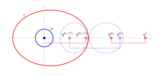
The $w$ contour is an arbitrarily small positively oriented circle around $0$, and the $z$ contour is positively oriented, goes around $q^{p_{2}+t_{2}},q^{p_{2}+t_{2}+1},q^{p_{2}+t_{2}+2},\ldots$ and the $w$ contour, and encircles no other $z$ poles of the integrand. The singularities of the integrand are as follows (see Figure 8 for an illustration):

1. In $w$, there is an essential singularity at $w=0$, and all the simple poles are at

   $$w=z\quad\textnormal{and}\quad w\in\bigl{\{}q^{p_{1}+j}\bigr{\}}_{j=0}^{t_{1}}\bigcap\hskip 1.0pt\bigl{\{}q^{x_{r}}\bigr{\}}_{r=1}^{m}.$$ (5.16)

2. In $z$, all the simple poles are at

   $$z=w\quad\textnormal{and}\quad z\in\bigl{\{}q^{j}\bigr{\}}_{j=0}^{\infty}\setminus\left(\bigr{\{}q^{p_{2}+j}\bigr{\}}_{j=1}^{t_{2}-1}\bigcup\hskip 1.0pt\bigl{\{}q^{x_{r}}\bigr{\}}_{r=1}^{m}\right).$$ (5.17)

Note that $z=0$ is not a pole thanks to the presence of the function $(z^{-1};q)_{\infty}$ in the denominator. Moreover, observe that at infinity, the integrand behaves as $O(w^{-2})$ as a function of $w$. This implies that it has no residue at $w=\infty$.

Figure 8: Thick curves represent the original $w$ and $z$ contours in $K_{\mathrm{walks}}$ (5.15). The possible $w$ poles (5.16) lie between $q^{p_{1}}$ and $q^{p_{1}+t_{1}}$. The possible $z$ poles (5.17) lie outside of the segment between $q^{p_{2}+1}$ and $q^{p_{2}+t_{2}-1}$. Note that the relative positions of $p_{1}$ and $p_{2}$, as well as of $p_{1}+t_{1}$ and $p_{2}+t_{2}$, may be arbitrary, and in the figure we display only one such possibility. The union of the dashed curves is the new $w$ contour after we drag it through infinity.

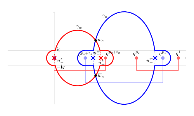
In the bulk asymptotic regime (5.1)–(5.2), assume that the position $(\tau,\rho)$ is in the liquid region $\mathcal{D}$ (Definition 5.3). We aim to deform the contours in $K_{\mathrm{walks}}$ (5.15) to new contours which intersect at the non-real critical points $w_{c},\overline{w}_{c}$, and coincide with the steepest descent contours $\gamma_{z},\gamma_{w}$ (defined before Lemma 5.6) outside a small neighborhood of the real line. Fix small $\varepsilon>0$, and perform the contour deformations in the following order:

1. Keeping the $w$ contour a small circle around $0$ of radius $\varepsilon/2$, deform the $z$ contour to coincide with the steepest descent contour $\gamma_{z}$ outside of the $\varepsilon$-neighborhood of $\mathbb{R}$. In the $\varepsilon$-neighborhood of $\mathbb{R}$, we need to make sure that the deformation from the old to the new $z$ contour does not cross any $z$-poles of the integrand. Namely, in the $\varepsilon$-neighborhood of $u^{z}_{-}=0$, let the new $z$ contour pass around $0$ following a circle of radius $\varepsilon$ instead of going straight to $0$ along $\gamma_{z}$. Around $u^{z}_{+}$ which is between $e^{-\gamma(\tau+\rho)}$ and $e^{-\gamma\rho}$ (see (5.14)) but may not be between $q^{p_{2}+t_{2}}$ and $q^{p_{2}}$, let the new $z$ contour follow straight lines at distance $\varepsilon$ from $\mathbb{R}$, and then go around the existing poles at distance at least $\varepsilon$ from these poles (see Figure 9 for an illustration). Denote the new $z$ contour by $\gamma_{z}^{\varepsilon}$.

2. Drag $w$ through infinity, that is, replace the $w$ integral over a small contour around $0$ by minus the integral over all the other $w$-poles which are listed in (5.16). Thus, we obtain minus the integral over the union of the dashed contours in Figure 8, minus $2\pi\mathbf{i}$ times the residue of the integrand at $w=z$ (which is still under the single integral in $z$ over $\gamma_{z}^{\varepsilon}$).

3. Now let us deform the $w$ contour to the steepest descent contour $\gamma_{w}$ outside the $\varepsilon$-neighborhood of $\mathbb{R}$. In the $\varepsilon$-neighborhood of $\mathbb{R}$ let us modify the new $w$ contour so that the deformation does not pick any residues one the real line, at points $w=q^{j}$ (this is done similarly to the contour $\gamma_{z}^{\varepsilon}$, see Figure 9 for an illustration). Denote the new $w$ contour by $\gamma_{w}^{\varepsilon}$. The deformation of the $w$ contour to $\gamma_{w}^{\varepsilon}$ picks a residue at $w=z$ if $z$ is in the right part of its contour, from $\overline{w}_{c}$ to $w_{c}$ in the counterclockwise order.

Accounting for all residues and sign changes throughout the contour deformation, we see that the kernel $K_{\mathrm{walks}}$ (5.15) takes the form:

$$\begin{split}&K_{\mathrm{walks}}(p_{1},t_{1};p_{2},t_{2})=-\mathbf{1}_{t_{2}>t_{1}}\mathbf{1}_{p_{2}+t_{2}>p_{1}+t_{1}}\frac{q^{(t_{1}-t_{2})(p_{1}+t_{1})}(q^{p_{1}-p_{2}+t_{1}-t_{2}+1};q)_{t_{2}-t_{1}-1}}{(q;q)_{t_{2}-t_{1}-1}}\\ &\hskip 20.0pt+\mathbf{1}_{t_{1}=t_{2}}\mathbf{1}_{p_{1}=p_{2}}+\frac{q^{-t_{1}-p_{1}}}{2\pi\mathbf{i}}\int_{w_{c}\to\overline{w}_{c}}\frac{z^{t_{1}-t_{2}}(q;q)_{t_{1}}(zq^{1-p_{2}-t_{2}};q)_{t_{2}-1}}{(q;q)_{t_{2}-1}(zq^{-p_{1}-t_{1}};q)_{t_{1}+1}}\hskip 1.0ptdz\\ &\hskip 20.0pt+\frac{q^{-t_{1}-p_{1}}}{(2\pi\mathbf{i})^{2}}\oint_{\gamma_{z}^{\varepsilon}}dz\oint_{\gamma_{w}^{\varepsilon}}dw\hskip 1.0pt\frac{(q;q)_{t_{1}}}{(q;q)_{t_{2}-1}}\frac{\exp\left\{m\left(S_{m}(w;t_{1},p_{1})-S_{m}(z;t_{2},p_{2})\right)\right\}}{(w-z)(1-zq^{-p_{2}})(1-zq^{-p_{2}-t_{2}})},\end{split}$$ (5.18)

Here the single integral is over the left part of the contour $\gamma_{z}^{\varepsilon}$, from $w_{c}$ to $\overline{w}_{c}$ in the counterclockwise order, and we used the notation (5.4).

Figure 9: Deformed integration contours to the steepest descent ones, with modifications in the $\varepsilon$-neighborhood of the real line to avoid picking unnecessary residues. Note that for large $m$, not all four modifications in the $\varepsilon$-neighborhood are present.

Lemma 5.7.

With $\varepsilon=m^{-1}$, in the bulk limit regime (5.1)–(5.2), the double contour integral in (5.18) goes to zero.

Proof.

All the quantities except $\exp\left\{m\left(S_{m}(w;t_{1},p_{1})-S_{m}(z;t_{2},p_{2})\right)\right\}$ in the double contour integral stay bounded in our limit regime. By Lemma 5.1, the functions $S_{m}$ are well-approximated by $S$. Since the integration contours are steepest descent for $S$ outside the $\varepsilon$-neighborhood of $\mathbb{R}$, we see that the contribution from the parts of the contours away from the real line goes to zero. This is because outside a small neighborhood of $w_{c}$ and $\overline{w}_{c}$, the integrand is bounded in absolute value by $e^{-cm}$ for some $c>0$.

To estimate the contribution from the neighborhood of the real line, we need to bound the derivative of $\mathop{\mathrm{Re}}S(w;\tau,\rho)$ along the straight and the circular parts of the additional contours. All of these non-steepest descent additional contours have length of order $\varepsilon=m^{-1}$. Indeed, for example, an additional contour may go from $q^{p_{1}}$ to $u_{+}^{w}$, and because $u_{+}^{w}>e^{-\gamma\rho}$, the length of this contour is bounded from above by the distance between $q^{p_{1}}$ and $e^{-\gamma\rho}$. This distance is of order $1/m$, see (5.1). Thus, it suffices to bound the derivative of $\mathop{\mathrm{Re}}S(w;\tau,\rho)$ on the additional contours by $o(m^{1-\delta})$ for some $\delta>0$. Indeed, then the total change of $\mathop{\mathrm{Re}}S(w;\tau,\rho)$ along the non-steepest descent additional contours is of order $o(m^{-\delta})$, and $e^{m(-c+o(m^{-\delta}))}$ still goes to zero exponentially fast.

To estimate the derivative of the real part of a function $f(z)=u(x,y)+iv(x,y)$ which is holomorphic in a neighborhood of a curve $z(\theta)=(x(\theta),y(\theta))$, we have by the Cauchy–Riemann equations:

$$\frac{\partial}{\partial\theta}\mathop{\mathrm{Re}}f(z(\theta))=x^{\prime}(\theta)\mathop{\mathrm{Re}}f^{\prime}(z(\theta))-y^{\prime}(\theta)\mathop{\mathrm{Im}}f^{\prime}(z(\theta)).$$

Let us now turn to the function $S(w;\tau,\rho)$ (5.8). Different summands in (5.8) have different singularities, let us consider each of these singularities in order. First, in a neighborhood of $u^{z}_{-}=0$ the modified contour $w(\theta)=\varepsilon e^{\mathbf{i}\theta}$ goes in a circular way without straight parts. We have (here and below in the proof, $C$ denotes a fixed sufficiently large positive constant whose value may differ from one inequality to the next):

$$\frac{\partial}{\partial\theta}\mathop{\mathrm{Re}}\bigl{(}\log w(\theta)\bigr{)}=0,\qquad\left|\frac{\partial}{\partial\theta}\mathop{\mathrm{Re}}\bigl{(}\mathrm{Li}_{2}(Aw(\theta)^{-1})\bigr{)}\right|\leq C,$$

for any $A>0$, and all other summands in (5.8) are regular around $0$.

The next singularities may appear in the neighborhoods of $u^{w}_{\pm}$ or $u^{z}_{+}$. In these neighborhoods, the modified contours may contain straight lines and circular segments. By changing variables, it suffices to estimate only the derivatives of the real parts of $\mathrm{Li}_{2}(w)$ and $\mathrm{Li}_{2}(w^{-1})$ in the neighborhood of $w=1$ (at all other points except $w=0$ these functions are regular, and we already considered $w=0$ above in the proof). We have for the circular contours $w(\theta)=1+\varepsilon e^{\mathbf{i}\theta}$:

$$\left|\frac{\partial}{\partial\theta}\mathop{\mathrm{Re}}\bigl{(}\mathrm{Li}_{2}(w(\theta))\bigr{)}\right|\leq C\varepsilon\log(\varepsilon^{-1}),\qquad\left|\frac{\partial}{\partial\theta}\mathop{\mathrm{Re}}\bigl{(}\mathrm{Li}_{2}(w(\theta)^{-1})\bigr{)}\right|\leq C\varepsilon\log(\varepsilon^{-1}),$$

For the straight contours $w(x)=x\pm\mathbf{i}\varepsilon$ we have:

$$\left|\frac{\partial}{\partial x}\mathop{\mathrm{Re}}\bigl{(}\mathrm{Li}_{2}(w(x))\bigr{)}\right|\leq C\log(\varepsilon^{-1}),\qquad\left|\frac{\partial}{\partial x}\mathop{\mathrm{Re}}\bigl{(}\mathrm{Li}_{2}(w(x)^{-1})\bigr{)}\right|\leq C\log(\varepsilon^{-1}),$$

We see that the derivative of $\mathop{\mathrm{Re}}S(w;\tau,\rho)$ is upper bounded (in the absolute value) by $C\log(\varepsilon^{-1})=C\log m$, which is $o(m^{1-\delta})$ for any $\delta<1$. This completes the proof. ∎

It remains to compute the limit of all the other terms in the right-hand side of (5.18) except the negligible double integral:

Lemma 5.8.

In the bulk limit regime (5.1)–(5.2), the sum of the first three terms in (5.18) converges to

$$(-1)^{\Delta t}e^{-\gamma(\tau+\rho)\Delta t}\left(\mathbf{1}_{t_{1}=t_{2}}\mathbf{1}_{p_{1}=p_{2}}-\mathsf{B}_{\omega}(t_{1}-t_{2},p_{1}-p_{2})\right),$$

where $\mathsf{B}_{\omega}$ is the incomplete beta kernel (Definition 2.11), and

$$\omega=\omega(\tau,\rho)\coloneqq\frac{1-w_{c}(\tau,\rho)e^{\gamma\rho}}{1-w_{c}(\tau,\rho)e^{\gamma(\tau+\rho)}},$$ (5.19)

where $w_{c}(\tau,\rho)$ is the critical point of $S(w;\tau,\rho)$ (5.8) in the upper half-plane (see Lemma 5.2).

The factor $(-1)^{\Delta t}e^{-\gamma(\tau+\rho)\Delta t}$ is simply a gauge transformation of the kernel which does not change a determinantal process.

Proof of Lemma 5.8.

Recall that the quantities $\Delta t=t_{1}-t_{2}$, $\Delta p=p_{1}-p_{2}$ are fixed. The first three terms in the right-hand side of (5.18) have the form

$$\begin{split}&\mathbf{1}_{\Delta t=\Delta p=0}-\mathbf{1}_{\Delta t<0}\mathbf{1}_{\Delta t+\Delta p<0}\frac{q^{\Delta t(p_{1}+t_{1})}(q^{\Delta t+\Delta p+1};q)_{-\Delta t-1}}{(q;q)_{-\Delta t-1}}\\ &\hskip 120.0pt+\frac{q^{-t_{1}-p_{1}}}{2\pi\mathbf{i}}\int_{w_{c}\to\overline{w}_{c}}\frac{z^{\Delta t}(q;q)_{t_{2}+\Delta t}(zq^{1-p_{2}-t_{2}};q)_{t_{2}-1}}{(q;q)_{t_{2}-1}(zq^{-p_{2}-t_{2}-\Delta p-\Delta t};q)_{t_{2}+\Delta t+1}}\hskip 1.0ptdz.\end{split}$$ (5.20)

Here the integration arc is the left part of the contour, from $w_{c}$ to $\overline{w}_{c}$ in the counterclockwise order.

We have for $\Delta t<0$ and $\Delta t+\Delta p<0$:

$$\frac{q^{\Delta t(p_{1}+t_{1})}(q^{\Delta t+\Delta p+1};q)_{-\Delta t-1}}{(q;q)_{-\Delta t-1}}\to(-1)^{-\Delta t-1}e^{-\gamma(\tau+\rho)\Delta t}\binom{-\Delta t-\Delta p-1}{-\Delta t-1}.$$

Indeed, this is because $\frac{1-q^{a}}{1-q^{b}}\to\frac{a}{b}$ for fixed $a,b\in\mathbb{Z}_{\geq 1}$ as $q\to 1$.

In the integrand, we have

$$\frac{(q;q)_{t_{2}+\Delta t}}{(q;q)_{t_{2}-1}}=(q^{t_{2}};q)_{\Delta t+1}\to(1-e^{-\gamma\tau})^{\Delta t+1},$$

using the standard notation of the $q$-Pochhammer symbol $(a;q)_{-k}=(aq^{-k};q)_{k}^{-1}$, $k\in\mathbb{Z}_{\geq 0}$, with a negative index. Similarly,

$$\frac{(zq^{1-p_{2}-t_{2}};q)_{t_{2}-1}}{(zq^{-p_{2}-t_{2}-\Delta p-\Delta t};q)_{t_{2}+\Delta t+1}}\\ =\frac{(zq^{1-p_{2}-\Delta p};q)_{\Delta p-1}}{(zq^{-p_{2}-t_{2}-\Delta p-\Delta t};q)_{\Delta t+\Delta p+1}}\to\bigl{(}1-ze^{\gamma\rho}\bigr{)}^{\Delta p-1}\bigl{(}1-ze^{\gamma(\tau+\rho)}\bigr{)}^{-\Delta t-\Delta p-1}.$$

Let us make a change of variables

$$u=\frac{1-ze^{\gamma\rho}}{1-ze^{\gamma(\tau+\rho)}},\qquad z=e^{-\gamma\rho}\hskip 1.0pt\frac{1-u}{1-e^{\gamma\tau}u},\qquad dz=-e^{-\gamma\rho}\frac{1-e^{\gamma\tau}}{(1-e^{\gamma\tau}u)^{2}}\hskip 1.0ptdu.$$

With this change of variables, (5.20) converges to

$$\begin{split}\mathbf{1}_{\Delta t=\Delta p=0}&+\mathbf{1}_{\Delta t<0}\mathbf{1}_{\Delta t+\Delta p<0}(-1)^{\Delta t}e^{-\gamma(\tau+\rho)\Delta t}\binom{-\Delta t-\Delta p-1}{-\Delta t-1}\\ &+\frac{(-1)^{\Delta t}e^{-\gamma(\tau+\rho)\Delta t}}{2\pi\mathbf{i}}\int_{\omega\to\overline{\omega}}(1-u)^{\Delta t}u^{\Delta p-1}\hskip 1.0ptdu,\end{split}$$ (5.21)

where $\omega$ is given by (5.19), and this point is in the upper half-plane. The integration arc goes from $\omega$ to $\overline{\omega}$ and crosses the real line between $0$ and $1$.

In (5.21), we can remove the overall factor $(-1)^{\Delta t}e^{-\gamma(\tau+\rho)\Delta t}$ as it is a gauge transformation leading to an equivalent determinantal kernel. Finally, for $\Delta t<0$, let us write

$$\frac{1}{2\pi\mathbf{i}}\int_{\omega\to\overline{\omega}}(1-u)^{\Delta t}u^{\Delta p-1}\hskip 1.0ptdu=-\mathop{\mathrm{Res}}\nolimits_{u=0}(1-u)^{\Delta t}u^{\Delta p-1}-\frac{1}{2\pi\mathbf{i}}\int_{\overline{\omega}}^{\omega}(1-u)^{\Delta t}u^{\Delta p-1}\hskip 1.0ptdu,$$

where the integration arc from $\overline{\omega}$ to $\omega$ in the right-hand side crosses the real line to the left of $0$. One readily sees that the minus residue at $u=0$ exactly cancels out with the second summand in (5.21). For $\Delta t\geq 0$, the integral in (5.21) is equal to $-\frac{1}{2\pi\mathbf{i}}\int_{\overline{\omega}}^{\omega}(1-u)^{\Delta t}u^{\Delta p-1}\hskip 1.0ptdu$, where the integration arc from $\overline{\omega}$ to $\omega$ crosses the real line between $0$ and $1$. This completes the proof. ∎

The contour deformations in the kernel $K_{\mathrm{walks}}$ (5.15) and Lemmas 5.8 and 5.7 complete the proof of Theorem 2.12.

University of Virginia, Charlottesville, VA, USA

E-mail: lenia.petrov@gmail.com

E-mail: me@mtikhonov.com

References

- [Agg19] A. Aggarwal. Universality for Lozenge Tiling Local Statistics. arXiv preprint, 2019. arXiv:1907.09991 [math.PR].
- [BG13] A. Borodin and V. Gorin. Markov processes of infinitely many nonintersecting random walks. Probab. Theory Relat. Fields, 155(3-4):935–997, 2013. arXiv:1106.1299 [math.PR].
- [BGR10] A. Borodin, V. Gorin, and E. Rains. q-Distributions on boxed plane partitions. Selecta Math., 16(4):731–789, 2010. arXiv:0905.0679 [math-ph].
- [BKMM07] J. Baik, T. Kriecherbauer, K. T.-R. McLaughlin, and P. D. Miller. Discrete Orthogonal Polynomials: Asymptotics and Applications. Annals of Mathematics Studies. Princeton University Press, 2007. arXiv:math/0310278 [math.CA].
- [BOO00] A. Borodin, A. Okounkov, and G. Olshanski. Asymptotics of Plancherel measures for symmetric groups. Jour. AMS, 13(3):481–515, 2000. arXiv:math/9905032 [math.CO].
- [Bor11] A. Borodin. Determinantal point processes. In G. Akemann, J. Baik, and P. Di Francesco, editors, Oxford Handbook of Random Matrix Theory. Oxford University Press, 2011. arXiv:0911.1153 [math.PR].
- [CIW19] P. Caputo, D. Ioffe, and V. Wachtel. Confinement of Brownian polymers under geometric area tilts. Electronic Journal of Probability, 24(none):1 – 21, 2019. arXiv:1809.03209 [math.PR].
- [CK01] R. Cerf and R. Kenyon. The low-temperature expansion of the Wulff crystal in the 3D Ising model. Comm. Math. Phys., 222:147–179, 2001.
- [CKP01] H. Cohn, R. Kenyon, and J. Propp. A variational principle for domino tilings. Jour. AMS, 14(2):297–346, 2001. arXiv:math/0008220 [math.CO].
- [DFG19] P. Di Francesco and E. Guitter. A tangent method derivation of the arctic curve for q-weighted paths with arbitrary starting points. Jour. Phys. A, 52(11):115205, 2019. arXiv:1810.07936 [math-ph].
- [DLMF] NIST Digital Library of Mathematical Functions. http://dlmf.nist.gov/, Release 1.1.8 of 2022-12-15. F. W. J. Olver, A. B. Olde Daalhuis, D. W. Lozier, B. I. Schneider, R. F. Boisvert, C. W. Clark, B. R. Miller, B. V. Saunders, H. S. Cohl, and M. A. McClain, eds.
- [DM15] E. Duse and A. Metcalfe. Asymptotic geometry of discrete interlaced patterns: Part I. Intern. J. Math., 26(11):1550093, 2015. arXiv:1412.6653 [math.PR].
- [DM20] E Duse and A. Metcalfe. Asymptotic Geometry of Discrete Interlaced Patterns: Part II. Annales de l’Institut Fourier, 70(1):375–436, 2020. arXiv:1507.00467 [math-ph].
- [Doo84] J.L. Doob. Classical potential theory and its probabilistic counterpart. Springer, 1984.
- [Dys62] F.J. Dyson. A Brownian motion model for the eigenvalues of a random matrix. Jour. Math. Phys., 3(6):1191–1198, 1962.
- [FS23] P.L. Ferrari and S. Shlosman. The Airy2 process and the 3D Ising model. Journal of Physics A: Mathematical and Theoretical, 56(1):014003, 2023. arXiv:2209.14047 [math.PR].
- [GH22] V. Gorin and J. Huang. Dynamical Loop Equation. arXiv preprint, 2022. arXiv:2205.15785 [math.PR].
- [GO09] A. Gnedin and G. Olshanski. A q-analogue of de Finetti’s theorem. El. Jour. Combin., 16:R16, 2009. arXiv:0905.0367 [math.PR].
- [Gor08] V. Gorin. Nonintersecting paths and the Hahn orthogonal polynomial ensemble. Funct. Anal. Appl., 42(3):180–197, 2008. arXiv:0708.2349 [math.PR].
- [Gor21] V. Gorin. Lectures on random lozenge tilings. Cambridge Studies in Advanced Mathematics. Cambridge University Press, 2021.
- [GP19] V. Gorin and L. Petrov. Universality of local statistics for noncolliding random walks. Ann. Probab., 47(5):2686–2753, 2019. arXiv:1608.03243 [math.PR].
- [Hay56] W.K. Hayman. A generalization of Stirling’s formula. J. Reine Angew. Math., 196:67–95, 1956.
- [Hua21] J. Huang. -Nonintersecting Poisson Random Walks: Law of Large Numbers and Central Limit Theorems. Intern. Math. Research Notices, 2021(8):5898–5942, 2021. arXiv:1708.07115 [math.PR].
- [Kas67] P. Kasteleyn. Graph theory and crystal physics. In Graph Theory and Theoretical Physics, pages 43–110. Academic Press, London, 1967.
- [Ken97] R. Kenyon. Local statistics of lattice dimers. Annales de Inst. H. Poincaré, Probabilités et Statistiques, 33:591–618, 1997. arXiv:math/0105054 [math.CO].
- [Ken09] R. Kenyon. Lectures on dimers. 2009. arXiv:0910.3129 [math.PR].
- [KM59] S. Karlin and J. McGregor. Coincidence probabilities. Pacific J. Math., 9:1141–1164, 1959.
- [KO07] R. Kenyon and A. Okounkov. Limit shapes and the complex Burgers equation. Acta Math., 199(2):263–302, 2007. arXiv:math-ph/0507007.
- [KOR02] W. König, N. O’Connell, and S. Roch. Non-colliding random walks, tandem queues, and discrete orthogonal polynomial ensembles. Electron. J. Probab., 7(5):1–24, 2002.
- [KOS06] R. Kenyon, A. Okounkov, and S. Sheffield. Dimers and amoebae. Ann. Math., 163:1019–1056, 2006. arXiv:math-ph/0311005.
- [LT15] B. Laslier and F. Toninelli. Lozenge tilings, Glauber dynamics and macroscopic shape. Comm. Math. Phys, 338(3):1287–1326, 2015. arXiv:1310.5844 [math.PR].
- [Mut06] L. Mutafchiev. The size of the largest part of random plane partitions of large integers. Integers: Electronic Journal of Combinatorial Number Theory, 6:A13, 2006.
- [Oko02] A. Okounkov. Symmetric functions and random partitions. In S. Fomin, editor, Symmetric functions 2001: Surveys of Developments and Perspectives. Kluwer Academic Publishers, 2002. arXiv:math/0309074 [math.CO].
- [OR03] A. Okounkov and N. Reshetikhin. Correlation function of Schur process with application to local geometry of a random 3-dimensional Young diagram. Jour. AMS, 16(3):581–603, 2003. arXiv:math/0107056 [math.CO].
- [OR07] A. Okounkov and N. Reshetikhin. Random skew plane partitions and the Pearcey process. Commun. Math. Phys., 269(3):571–609, 2007. arXiv:math/0503508 [math.CO].
- [Pet14] L. Petrov. Asymptotics of Random Lozenge Tilings via Gelfand-Tsetlin Schemes. Probab. Theory Relat. Fields, 160(3):429–487, 2014. arXiv:1202.3901 [math.PR].
- [Pet15] L. Petrov. Asymptotics of Uniformly Random Lozenge Tilings of Polygons. Gaussian Free Field. Ann. Probab., 43(1):1–43, 2015. arXiv:1206.5123 [math.PR].
- [Pet22] L. Petrov. Noncolliding Macdonald walks with an absorbing wall. SIGMA, 18:21, 2022. arXiv:2204.09206 [math.PR].
- [She05] S. Sheffield. Random surfaces. Astérisque, 304, 2005. arXiv:math/0304049 [math.PR].
- [TF61] H. Temperley and M. Fisher. Dimer problem in statistical mechanics - an exact result. Philos. Mag., 6(68):1061–1063, 1961.