PipeLearn: Pipeline Parallelism for
Collaborative Machine Learning
Abstract
Collaborative machine learning (CML) techniques, such as federated learning, were proposed to collaboratively train deep learning models using multiple end-user devices and a server. CML techniques preserve the privacy of end-users as it does not require user data to be transferred to the server. Instead, local models are trained and shared with the server. However, the low resource utilisation of CML techniques makes the training process inefficient, thereby limiting the use of CML in the real world. Idling resources both on the server and devices due to sequential computation and communication is the principal cause of low resource utilisation. A novel framework PipeLearn that leverages pipeline parallelism for CML techniques is developed to improve resource utilisation substantially. A new training pipeline is designed to parallelise the computations on different hardware resources and communication on different bandwidth resources, thereby accelerating the training process in CML. The pipeline is further optimised to ensure maximum utilisation of available resources. The experimental results confirm the validity of the underlying approach of PipeLearn and highlight that when compared to federated learning: (i) the idle time of the server can be reduced by 2.2x – 28.5x, (ii) the network throughput can be increased by 56.6x – 321.3x, and (iii) the overall training time can be accelerated by 1.5x – 21.6x under varying network conditions for two popular convolutional models without sacrificing accuracy. PipeLearn is available for public download from https://github.com/blessonvar/PipeLearn.
Index Terms:
Collaborative machine learning, resource utilisation, pipeline parallelism, edge computing.I Introduction
Deep learning has found application across a range of fields, including computer vision [1, 2], natural language processing [3, 4] and speech recognition [5, 6]. However, there are important data privacy and regulatory concerns in sending data generated on devices to geographically distant cloud servers for training deep learning models. A new class of machine learning techniques has therefore been developed under the umbrella of collaborative machine learning (CML) to mitigate these concerns [7]. CML does not require data to be sent to a server for training deep learning models. Rather the server shares models with devices that are then locally trained on the device.
There are three notable CML techniques, namely federated learning (FL) [8, 9, 10, 11], split learning (SL) [12, 13] and split federated learning (SFL) [14, 15]. However, these techniques are performance inefficient since they under-utilise resources (both compute and network), which results in training times that are impractical for real-world use. The cause of resource under-utilisation in the three CML techniques is considered next.
In FL, each device trains a local model of a deep neural network (DNN) using the data it generates. Local models are uploaded to the server and aggregated as a global model at a pre-defined frequency. However, the workload of the devices and the server is usually imbalanced [16, 17, 15]. This is because the server resources are only employed when the local models are aggregated and remain idle for the remaining time.
In SL, a DNN is usually decomposed into two parts, such that the initial layers of the DNN are deployed on a device and the remaining layers on the server. A device trains the partial model and sends the intermediate outputs to the server where the rest of the model is trained. The training of the model on devices occurs in a round-robin fashion. Hence, only one device or the server will utilise its resources while the other devices or server are idle [14, 7].
In SFL, which is a hybrid of FL and SL, the DNN is split across devices and the server; the devices, however, unlike SL, train the local models concurrently. Nevertheless, the server is required to wait while the devices train the model and transfer data, and vice versa.
Therefore, the following two challenges need to be addressed for improving the resource utilisation of CML techniques:
a) Sequential execution on devices and server causes resource under-utilisation: Since device-side and server-side computations in CML techniques occur in sequence, there are long idle times on both the devices and server.
b) Communication between devices and server results in resource under-utilisation: Data transfer in CML techniques is time-consuming [18, 19, 20], during which time no training occurs on both the server and devices. This increases the overall training time.
Although low resource utilisation of CML techniques makes training inefficient, there is currently limited research that is directed at addressing this problem. The motivation of this paper is to address the above challenges by developing a framework, PipeLearn, that leverages pipeline parallelism to improve the resource utilisation of devices and servers in CML techniques when training DNNs, thereby increasing training efficiency. The framework distributes the computation of DNN layers on the server and devices, balances the workload on both the server and devices, and reorders the computation for different inputs in the training process. PipeLearn overlaps the device and server-side computation and communication between the devices and server, thereby improving resource utilisation, which accelerates CML training.
PipeLearn redesigns the training process of DNNs. Traditionally, training a DNN involves the forward propagation pass (or forward pass) and backward propagation pass (or backward pass). In the forward pass, one batch of input data (also known as a mini-batch) is used as input for the first input layer and the output of each layer is passed on to subsequent layers to compute the loss function. In the backward pass, the loss function is passed from the last DNN layer to the first layer to compute the gradients of the DNN model parameters.
PipeLearn divides the DNN into two parts and deploys them on the server and devices like in SFL. Then the forward and backward passes are reordered for multiple mini-batches. Each device executes the forward pass for multiple mini-batches in sequence. The immediate result of each forward pass (smashed data or activations) is transmitted to the server, which runs the forward and backward passes for the remaining layers and sends the gradients of the activations back to the device. The device then sequentially performs the backward passes for the mini-batches. The devices operate in parallel, and the local models are aggregated at a set frequency. Since many forward passes occur sequentially on the device, the communication for each forward pass overlaps the computation of the following forward passes. Also, in PipeLearn, the server and device computations occur simultaneously for different mini-batches. Thus, PipeLearn reduces the idle time of devices and servers by overlapping server and device-side computations and server-device communication.
This paper makes the following contributions:
-
1.
The development of a novel framework PipeLearn that accelerates collaborative training of DNNs by improving resource utilisation. To the best of our knowledge, PipeLearn is the first work to reduce the idling of resources in CML by reordering training tasks across the server and devices.
-
2.
Pipeline parallelism is leveraged to the benefit of CML for the first time to overlap device and server computations and device-server communication, thereby reducing resource idle time. Experiments in a lab-based testbed demonstrate that, compared to FL, the training process can be accelerated by 1.5x - 21.6x, and the utilisation of idle hardware resources and bandwidth resources are increased by upto 28.5x and 321.3x.
-
3.
Development of an optimised strategy for partitioning and scheduling CML workloads across devices and servers to maximise overall training efficiency. Experimental studies demonstrate that our approach can find optimal or near-optimal strategies.
The remainder of this paper is organised as follows. Section II provides the background and related works of this research. The PipeLearn framework and the two approaches that underpin the framework are detailed in Section III. Experiments in Section IV demonstrates the effectiveness of the PipeLearn framework under varying network conditions. Section V concludes this article.
II Background and Related Work
Section II-A provides the background of collaborative machine learning (CML), and Section II-B introduces the related research on improving the training efficiency in CML.
II-A Background
The training process of the three popular CML techniques, namely federated learning (FL), split learning (SL) and split federated learning (SFL), and their limitation due to resource under-utilisation are presented.
II-A1 Federated Learning
FL [8, 9, 10, 11] uses a federation of devices coordinated by a central server to train deep learning models collaboratively.
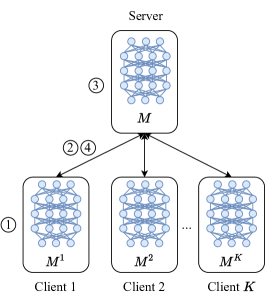
Assume devices are involved in the training process as shown in Figure 1(a). In Step ①, the devices train the complete model locally, where . In each iteration, the local model is fed a mini-batch of data, completes the forward and backward passes to compute gradients of all model parameters, and then updates the parameters with the gradients. A training epoch involves training over the entire dataset, which consists of multiple iterations. In Step ②, after a certain number of local epochs, the devices send the local models to the server, where . In Step ③, the server aggregates the local models to obtain a global model , using the FedAvg algorithm [11] , where is the local dataset on device and is the function to obtain the set size. In Step ④, the global model is then downloaded to the devices and continues the next round of training until the model converges.
Typically, local model training on devices (Step ①) takes most of the time, while the resources with better compute performance on the server are idle. Therefore, PipeLearn utilises the idle resources on the server during training.
II-A2 Split Learning
SL [12, 13] is another privacy-preserving CML method. Since a DNN consists of consecutive layers, SL splits the complete DNN into two parts at the granularity of layers and deploys them on the server () and the devices (, where ).
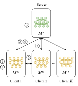
As shown in Figure 1(a), the devices train the initial layers of the DNN and the server trains the remaining layers, and the devices work in a round-robin fashion. In Step ①, the first device runs the forward pass of on its local data, and in Step ②, the intermediate results (also known as activations) are sent to the server. In Step ③, the server uses the activations to complete the forward pass of to obtain the loss. The loss is then used for the backward pass on the server to compute the gradients of the parameters of and the gradients of the activations. In Step ④, the gradients of the activations are sent back to the device, and in Step ⑤, the gradients of the parameters of the are computed in the device-side backward pass. Next, the parameters of server-side model and device-side model are updated by their gradients. In Step ⑥, after a device trains for a certain number of epochs, the next device gets the latest model from the previous device, and starts training its model in Step ⑦.
Compared to FL, the device-side computation is significantly reduced, because only a few layers are trained on devices. However, since the devices works in sequence (instead of in parallel as FL), the overall training efficiency decreases as the number of devices increases.
II-A3 Split Federated Learning
Since FL is computationally intensive on devices and SL works inefficiently on the device side, SFL [14] was developed to alleviate both limitations. Similar to SL, SFL also splits the DNN across the devices (, where ) and the server () and collaboratively trains the DNN. However, in SFL, the devices train in parallel and utilise a ‘Main’ server for training the server-side model and a ‘Fed’ server for aggregation.
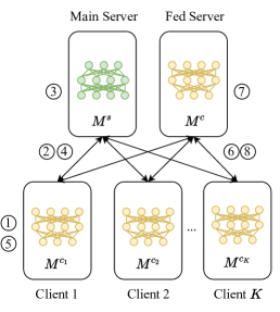
The training process is shown in Figure 1(b). In Step ①, the forward pass of , where , are executed on the devices in parallel, and in Step ②, the activations are uploaded to the main server. In Step ③, the main server trains , and in Step ④, the gradients are sent back to all devices, before they complete the backward pass in Step ⑤. At a pre-defined frequency, , where , are uploaded to the Fed server in Step ⑥. In Step ⑦, the models are aggregated to the global model . In Step ⑧, is downloaded to the devices and used for the next round of training.
SFL utilises device parallelism to improve the training efficiency of SL [7]. However, the server still waits while the devices are training the model (Step ①) and transmitting data (Step ②), and vice versa, which leads to resource under-utilisation. PipeLearn solves this problem by parallelising the steps performed on the server and the devices.
II-B Related work
Existing research aimed at improving the training efficiency of CML techniques focuses on the following four aspects.
II-B1 Accelerating Model Convergence
Model convergence is usually slow when the data from different devices is not independent and identically distributed (non-i.i.d). To mitigate this problem, recent works proposed new optimisation algorithms for federated learning. FedAc [21] reduced the rounds of synchronisation required for model convergence to one-third of FedAvg. FedReg [22] indicated that the slow convergence is mainly caused by a forgetting issue during the local training stage, and alleviated it by regularising local parameters with previous training data. Momentum [23] and weighting methods [24] were used in the gradient descent to accelerate convergence. Devices selection methods based on data similarity [25] and data distribution [26] were adopted in the aggregation stage to improve model convergence.
These methods accelerate the training process of CML techniques by improving model convergence. However, there is no focus on improving the resource utilisation of the server and devices by reducing idle time.
II-B2 Reducing the Impact of Stragglers
Stragglers among the devices participating in training increase the overall training time of CML techniques. A device selection method was proposed based on the resource conditions of devices to rule out the stragglers [27]. Some neurons in straggler’s model are masked to accelerate its computation [28]. Local gradients are aggregated hierarchically to accelerate FL for heterogeneous devices [29]. FedAdapt [15] balances the workloads on heterogeneous devices by offloading some layers of DNN to the server.
These methods alleviate the impact of stragglers but do not address the fundamental challenge of sequential computation and communication between the devices and server that results in low resource utilisation.
II-B3 Reducing Communication Overhead
In limited bandwidth environments, communication overhead limits the training efficiency of CML techniques. To reduce the communication traffic in FL, a relay-assisted two-tier network was used [30]. Models and gradients were transmitted simultaneously and aggregated on the relay nodes. Pruning, quantisation and selective updating were used to reduce the model size and thus reduce the computation and communication overhead [31]. The communication involved in the backward pass of SFL is improved by averaging the gradients on the server side and broadcasting them to the devices instead of unicasting the unique gradients to devices [32].
These methods are effective in reducing the volume of data transferred over the network, thus reducing the communication overhead. However, the network throughput (the volume of data transferred in a given time frame) remains unchanged since the network is not effectively used.
II-B4 Improving Resource Utilisation by Parallelisation
Although the above methods improve the training efficiency of CML techniques, they do not surmount the challenge of under-utilisation of resources. Parallelisation techniques have therefore been proposed to improve the utilisation of compute and bandwidth resources. GPipe [33] and PipeDream [34] proposed pipeline parallelism to distribute a deep model to multiple computing nodes and parallelise the computations on different nodes. Both reduced the idle time of computing resources. However, the network topology of computing nodes is sequential rather than centralised as in CML techniques, where all the raw data is fed into one node and flows to the others. Thus, they cannot be used in CML techniques where data resides on every device. In addition, they can only operate in a homogeneous environment, where all compute nodes have similar hardware and assumes the availability of significant computing power. Thus, they are less suitable for use in relatively resource-constrained IoT environments. Overlap-FedAvg [35] was proposed to decouple the computation and communication during training and overlap them to reduce idle resources. However, the use of computing resources located at the server is not fully leveraged.
Given the above limitations, we therefore, propose a novel framework PipeLearn that fully utilises the computing resources on the server and devices and the bandwidth resources between them, thereby significantly improving the training efficiency of CML.
III PipeLearn
This section develops PipeLearn, a framework that improves the resource utilisation of CML, such as in the context of FL and SFL. PipeLearn accelerates the execution of sequential DNNs for the first time by leveraging pipeline parallelism to improve the overall resource utilisation (of both compute and network) in centralised CML.
The PipeLearn framework is underpinned by two approaches, namely pipeline construction and pipeline optimisation. The first approach constructs a training pipeline to balance the overall training workload by (a) reallocating the computations for different layers in DNN on the server and devices, and (b) reordering the forward and backward passes for multiple mini-batches of data and schedules them onto idle resources. Consequently, not only is the resource utilisation improved by using PipeLearn, but also the overall training of the DNN is accelerated. The second approach of PipeLearn enhances the performance of the first approach by automatically selecting the optimal control parameters (such as the point at which the DNN must be split across the device and the server and the number of mini-batches that can be executed concurrently in the pipeline).
III-A Motivation
The following three observations in relation to low resource utilisation in the training process of DNNs in CML motivates the development of PipeLearn.
The server and devices need to work simultaneously: The devices and server work in an alternating manner in the current CML methods, which is a limitation that must be addressed for improving resource utilisation. In FL, the server starts to aggregate local models only after all devices have completed training their local models. In SL/SFL, the sequential computation of DNN layers results in the sequential working of the devices and the server. To reduce the resulting idle time on the resources, the dependencies between server-side and device-side computations need to be eliminated. PipeLearn attempts to make the server and the devices work simultaneously by reallocating and reordering training tasks.
Compute-intensive and I/O-intensive tasks need to be overlapped: Compute-intensive tasks, such as model training, involves large-scale computation that need to be performed by computing units (CPU/GPU), while IO-intensive tasks refer to input and output tasks of disk or network, such as data transmission, which usually do not have a high CPU requirement. A computationally intensive and an IO-intensive task can be executed in parallel on the same resource without mutual dependencies. However, in the current CML methods, both server-side and device-side computations are paused when communication is in progress, which creates idle time on compute resources. PipeLearn improves this by overlapping compute-intensive and IO-intensive tasks.
Workloads on the server side and client side need to be balanced: Idle time on resources are also caused due to unbalanced workloads on the server and devices. In current CML methods, servers or clients may have heavier workload than the other. PipeLearn balances the workloads on the server side and device side by split the neural network carefully.
III-B Pipeline Construction
Assume that devices and a server train a sequential DNN collaboratively by using data residing on each device. Conventionally, the dataset on each device is divided to multiple mini batches that is fed to the DNN in sequence. Training on each mini-batch involves a forward pass that computes a loss function and a backward pass that computes the gradients of the model parameters. A training epoch ends after the entire dataset has been fed to the DNN. To solve the problem of low resource utilisation faced by the current CML methods, PipeLearn constructs a training pipeline that reduces the idle time on resources during collaborative training.
Each forward and backward pass of CML methods comprises four tasks: (i) the device-side compute-intensive tasks, such as model training; (ii) the server-side compute-intensive task, such as model training (only in SL and SFL) and model aggregation; (iii) the device-to-server IO-intensive task, such as data uploading; (iv) the server-to-device IO-intensive task, such as data downloading. The four tasks can only executed in sequence in current CML methods, resulting in idle resources. To solve this problem, a pipeline is developed to balance and parallelise the above tasks. The pipeline construction approach involves three phases, namely neural network splitting, training stage reordering and multi-device parallelisation.
Phase 1 - Neural Network Splitting
The aim of the approach is to overlap the above four tasks to reduce idle time on computing resources on the server and devices as well as idle network resources. Since this approach does not reduce the actual computation and communication time in each task, it needs to balance the time required by the four tasks to avoid straggler tasks from increasing the overall training time. For example, in FL the device-side compute-intensive task is most time-consuming, while the other three tasks consume relatively less time. In this case, overlapping the four tasks will not significantly reduce the overall training time. Therefore, it is more suitable to split the DNN and divide the training task across the server and the devices (similar with the previous works [14, 15]). In addition, since the output of each DNN layer has a variable size, different split points of the DNN will result in different volumes of transmitted data. Thus, changing the splitting point based on the computing resources and bandwidth can also balance the I/O-intensive tasks with compute-intensive tasks. The selection of the best splitting point is presented in Section III-C.
Splitting neural networks does not affect model accuracy, since it does not alter computations rather the resource on which they are executed. In FL, each device , where , trains a complete model . PipeLearn splits to a device-side model and a server-side model represented as:
| (1) |
where the binary operator stacks the layers of two partitions of a deep learning model as a complete model.
There are pairs of , where is deployed on device while all of are deployed on the server. This is different from SL and SFL where only one model is deployed on the server side. Assume the complete model contains layers, contains the initial layers and contains the remaining layers, where .
Splitting the neural network maintains the consistency of the training process and does not change the model accuracy (refer to Appendix A in Supplementary Material).
Phase 2 - Training Stage Reordering
After splitting the neural networks and balancing the four tasks, the idle resources in the training process need to be utilised. This is achieved by reordering the computations for different mini-batches of data.
Figure 2(a) shows the pipeline of one training iteration of a split neural network for one pair of (the device index is not shown). Any forward pass (), backward pass (), upload task () and download task () for each mini-batch is called a training stage.
The idle time on the device exists between the forward pass and the backward pass of the device-side model. Thus, PipeLearn inserts the forward pass of the next few mini-batches into the device-side idle time to fill up the pipeline. As shown in Figure 2(b), in each training iteration, the forward passes for mini-batches, to , are performed on the device in sequence. The activations of each mini-batch are sent to the server ( to ) once the corresponding forward pass is completed, which utilises idle network resources. Once the activations of any mini-batch arrive, the server performs the forward and backward passes, to , and sends the gradients of the activations back to the device ( to ). After completing the forward passes of the mini-batches and receiving the gradients, the device performs the backward passes, to . Then the model parameters are updated and the training iteration ends. A training epoch ends when the entire dataset has been processed, which involves multiple training iterations.
Figure 2(b) shows that compared to conventional training (Figure 2(a)), the degree to which the four tasks can be overlapped is high and it is possible to significantly reduce the idle time of the server and the devices.


To guarantee a similar model accuracy as in classic FL, it must be ensured that the gradients are obtained from the same number of data samples when the model is updated. This requires that the number of data samples involved in each training iteration in PipeLearn should be the same as the original batch size in FL. Since mini-batches are used in each training iteration, the size of each mini-batch is reduced to of the original batch size in FL.
| (2) |
Reordering training stages does not impact model accuracy (refer to Appendix B in Supplementary Material).
Phase 3 - Multi-Device Parallelisation
The workloads of multiple devices involved in collaborative training needs to be coordinated. On the device side, each device is responsible for training its model , and PipeLearn allows them to train in parallel for efficiency. On the server side, the counterpart models ( to ) are deployed and trained simultaneously. However, this may result in compute resources contention.
Figure 3(a) shows the case of single device that is the same as Figure 2(b) but not shows communication, while Figure 3(b) and 3(c) shows the case of multiple devices. Figure 3(b) gives one straightforward solution to train the server-side models sequentially. However, the server-side models that are trained relatively late will cause a delay in the backward passes for the corresponding device-side models, for example, , where , in Figure 3(b).
Alternatively, data parallelism can be employed. The activations from different devices are deemed as different inputs and the server-side models are trained in parallel on these inputs. This is shown in Figure 3(c). It is worth noting that, compared to training a single model, training multiple models at the same time may result in longer training time for each model on a resource-limited server. This approach, nonetheless, mitigates stragglers on devices.


At the end of each training epoch, the device-side models are uploaded to the server, and will constitute the entire models when combined with the server-side models (Equation 1). The complete model of each device is aggregated to obtain a complete global model , using the FedAvg algorithm [11].
| (3) |
where is the local dataset on device and is the function to obtain the size of the given dataset. The server-side global model and device-side global model are split from , using
| (4) |
The devices download to update the local models for the subsequent training epochs, and the server-side models are updated by .
It has been proved in the previous phases that the model accuracy of each local model in PipeLearn is not affected. In this phase, the FedAvg algorithm is used in PipeLearn to generate the global model by aggregating , where , which is the same as in classic FL. Therefore, PipeLearn maintains similar model accuracy with FL.
Training Process Overview
All devices train simultaneously using Algorithm 1. On device , the device-side model is initially built given the split point (Line 1). Line 2 to Line 19 shows the complete training process until the model converges. In each training epoch (Line 3 to Line 18), the entire dataset is processed. A training epoch consists of multiple training iterations, each processing data samples. In each training iteration (Line 4 to Line 13), the forward passes of mini-batches are executed in sequence (Line 6), and the activations are sent to the server (Line 7). Their gradients are then received from the server (Line 10), and the backward passes are executed sequentially to compute the gradients of the weights of (Line 11). At the end of a training iteration, the model is updated based on the gradients (Line 13). After all training iterations are completed, the signal “stop epoch” and is sent to the server (Line 15 to Line 16). The device then receives a global device-side model from the server (Line 17) and uses it to update the current model (Line 18). When the model converges, the client sends a “stop training” signal to the server, thus completing the training process (Line 20).
Algorithm 2 is executed on the server side. The server first builds models , where (Line 1), and starts training the models until a signal “stop training” is received from all devices (Line 2). In each training epoch (Line 3 to Line 24), the models are trained simultaneously (Line 3 to Line 19) and aggregated into a global model (Line 20 to Line 23). A training epoch of model does not end until receive a signal “stop epoch” (Line 5) from device , which involves multiple training iterations. During a training iteration (Line 6 to Line 15), the server receives the activations and labels from device (Line 7), and uses them to compute the loss function (Line 9 to Line 10). After that, the gradients of activations and model weights are computed (Line 11 to Line 12). The former is then sent to device (Line 13), and the latter is used to update at the end of the training iteration (Line 15). After receiving the “stop epoch” signal, the server receives the device-side model from device (Line 17) and makes up a complete model (Line 18). The models , where , are aggregated into a global model (Line 20). is then split into a server-side model and a device side model (Line 21). is sent to device (Line 22), and is used to update (Line 23). A training epoch ends. Training is completed when the ”stop training” signal is received from all devices.
III-C Pipeline Optimisation
To ensure that the pipeline can efficiently utilise the idle resources, we propose an approach that optimises the pipeline. Two important parameters that significantly impact the performance of the pipeline need to be considered:
a) Split point: The split point of a neural network is denoted as . All layers with indices less than or equal to are deployed on the device and the remaining layers are deployed on the server. The number of layers determines the amount of computation on a server/device, and the volume of data output from the split layer determines the communication traffic. Therefore, finding the most suitable value for for each device will balance the time required for computation on the server and the device as well as the communication between them.
b) Parallel batch number: the number of mini-batches that are used to concurrently train the model in each iteration of training is called parallel batch number and denoted by . It is important that the computations for mini-batches fill up the pipeline. Therefore, it is necessary to decide the number of mini-batches involved in each training iteration.
The above two parameters, namely spilt point and parallel batch number, of the pipeline significantly influence the efficiency of PipeLearn, and the approach required for obtaining the optimal values for and is developed. These parameters will change for different DNNs, servers/devices combinations and network conditions. An exhaustive search for optimal values based on actual model training would be time and resource consuming. Therefore, the approach developed rely on estimating the training time for different parameters.
This approach aims to select the best pair of for each device to minimise the idle resources by three phases. Firstly, we need to know how much they affect the pipeline. A number of training iterations is profiled to identify size of the output data and the training time for each layer of the DNN. Secondly, the training time for each epoch can be estimated using the above information, given a pair of . Thirdly, the candidates for are shortlisted. Since the training time can be estimated for every candidate, the one with the lowest training time will be selected. The three phases are explained in detail as follows.
Phase 1 - Profiling
In this phase, the complete model is trained on each device and server for a pre-defined number of iterations. The following information is empirically collected:
a) Time spent in the forward/backward pass of each layer deployed on each device and server. Assume that , , and denote the forward and backward pass of layer on device and server, and denotes time. Then, , , and are the time taken for the forward and backward pass on the devices and server.
b) Output data volume of each layer in the forward and backward pass. and denote the output data volume for layer in forward and backward pass.
Phase 2 - Training Time Estimation
To estimate the time spent in each training epoch of , given the pairs of for device , where , the time for each training stage must be estimated first.
Assume that , , and is the time spent in the forward and backward pass of the and for mini-batch , where . The time spent in each stage is the sum of the time spent in all relevant layers. Since the size of each mini-batch in PipeLearn is reduced to , the time required for each layer is reduced to around . The time of each training stage is estimated by the following equations:
| (5) |
| (6) |
| (7) |
| (8) |
Assume that and are the time spent in uploading and downloading between device and the server for mini-batch , where , and and are the uplink and downlink bandwidths. Since the size of transmitted data is reduced to :
| (9) |
| (10) |
The time consumption of all training stages is estimated using the above equations, then the training time of each epoch can be estimated using dynamic programming. Within each training iteration, a training stage has previous stages and next stages (exclusions for first and last stages). Table I shows the previous and next stages of all stages in each training iteration. The first stage is and the last stage is . We use to denote the total time from the beginning of the training iteration to the end of the stage , and to denote the time spent in the stage . Thus, the overall training time is . Since any stage can start only if all of its previous stages have completed, we have
| (11) |
| (12) |
| (13) |
where is the function to obtain all previous stages of the input stage. Since is already obtained in Phase 2, Equation 11 to 13 can be solved by recursion. The overall time of one training iteration can then be estimated.
Phase 3 - Parameter Determination
In this phase, the candidates of are shortlisted. Since the training time can be estimated for each candidate, the one with lowest training time can be selected.
Assuming that the DNN has layers, including dense layers, convolutional layers, pooling layers, etc., the range of is , where is the set of all positive integers.
Given , the idle time of the device between the forward pass and backward pass of each mini-batch (the blank between and in Figure 2(a)), need to be filled up by the forward passes of the following multiple mini-batches. As a result, the original mini-batch and the following mini-batches are executed concurrently in one training iteration.
For example, as shown in Figure 2(a), the device idle time between and is equal to . Thus, the forward passes or backward passes of the subsequent mini-batches can be used to fill in the idle time, making the parallel batch number . Since the batch size used in PipeLearn is reduced to , the time required for forward and backward pass of each layer, uploading and downloading are reduced to around . The parallel batch number for device is estimated as:
| (14) |
For each device , the best can be selected from the shortlisted candidates by estimating the training time.
Since the training time of PipeLearn with parameter pair is estimated based on profiling data from training complete models with the original batch size, this approach does not guarantee to select the optimal parameters. However, our experiments in Section IV-D show that the parameters selected by this approach are similar to optimal values.
| Stage | Previous Stages | Next Stages |
|---|---|---|
| , | ||
| , | ||
| , | ||
| , | ||
| , | , | |
| , | ||
| , | ||
| , | ||
| , | ||
| , | ||
| , | ||
| , | , | |
| , | ||
| , | ||
| , | ||
| , |
IV Experiments
This section quantifies the benefits of PipeLearn and demonstrate its superiority over existing CML techniques. Therefore, the training efficiency (Section IV-B) and the model accuracy and convergence (Section IV-C) of PipeLearn are compared against existing CML techniques. The performance of the optimisation techniques is then evaluated in Section IV-D.
IV-A Experimental Setup
The test platform consists of one server and four devices. An 8-core i7-11850H processor with 32GB RAM is used as the server that collaboratively trains DNNs with four Raspberry Pi 3B devices each with 1GB RAM.
Three network conditions are considered: a) 4G: 10Mbps uplink bandwidth and 25Mbps downlink bandwidth; b) 4G+: 20Mbps uplink bandwidth and 40Mbps downlink bandwidth; c) WiFi: 50Mbps uplink bandwidth and 50Mbps downlink bandwidth.
The neural networks used in these experiments are VGG5 [36] and ResNet18 [37]. Their architectures are shown in Table II.“CONV-A-B-C” represents a convolutional layer with the kernel size of AA and the number of output channels B, followed by a pooling layer C if applicable. “MaxPool” and “AvgPool” denotes a max pooling layer and a average pooling layer, respectively. “FC-A” represents a fully connected layer with the output size A. “RES-A-B-C” denotes a residual block that consists of two convolutional layers with the kernel size of AA and the number of output channels B, followed by a pooling layer C if applicable. The output of each residual block is the output of the last inner convolutional layer plus the input of the residual block. For convenience, the activation functions and batch normalisation functions are not shown in the table.
| VGG5 | ResNet18 |
|---|---|
| CONV-3-32-MaxPool | CONV-7-64-MaxPool |
| CONV-3-64-MaxPool | RES-3-64 |
| CONV-3-64 | RES-3-64 |
| FC-128 | RES-3-128 |
| FC-10 | RES-3-128 |
| RES-3-256 | |
| RES-3-256 | |
| RES-3-512 | |
| RES-3-512-AvgPool | |
| FC-10 |
The dataset used in these experiments is CIFAR-10 [38, 39]. All images in CIFAR-10 have the shape of , and are classified into 10 classes. Each devices owns a training dataset with 10,000 data samples. The validation dataset and test dataset have 2000 and 8000 data samples, respectively. In the training process, the data samples are input into the neural network in form of mini batches. The size of each mini batch (batch size) is 100 for each device in FL and SFL. In PipeLearn, the batch size is , where is the parallel batch number for device and .
IV-B Efficiency Results
The experiments in this section compares the efficiency of PipeLearn with FL and SFL. Although SL is a popular CML technique, it is significantly slower than SFL since each device operates sequentially. Hence, SL is not considered in these experiments. All possible split points for SFL are benchmarked (similar to the benchmarking method adopted in Scission [40]), and the efficiency of SFL with the best split point is reported. The split point and parallel batch number for PipeLearn are selected by the optimisation technique proposed in Section III-C.
IV-B1 Comparing Efficiency
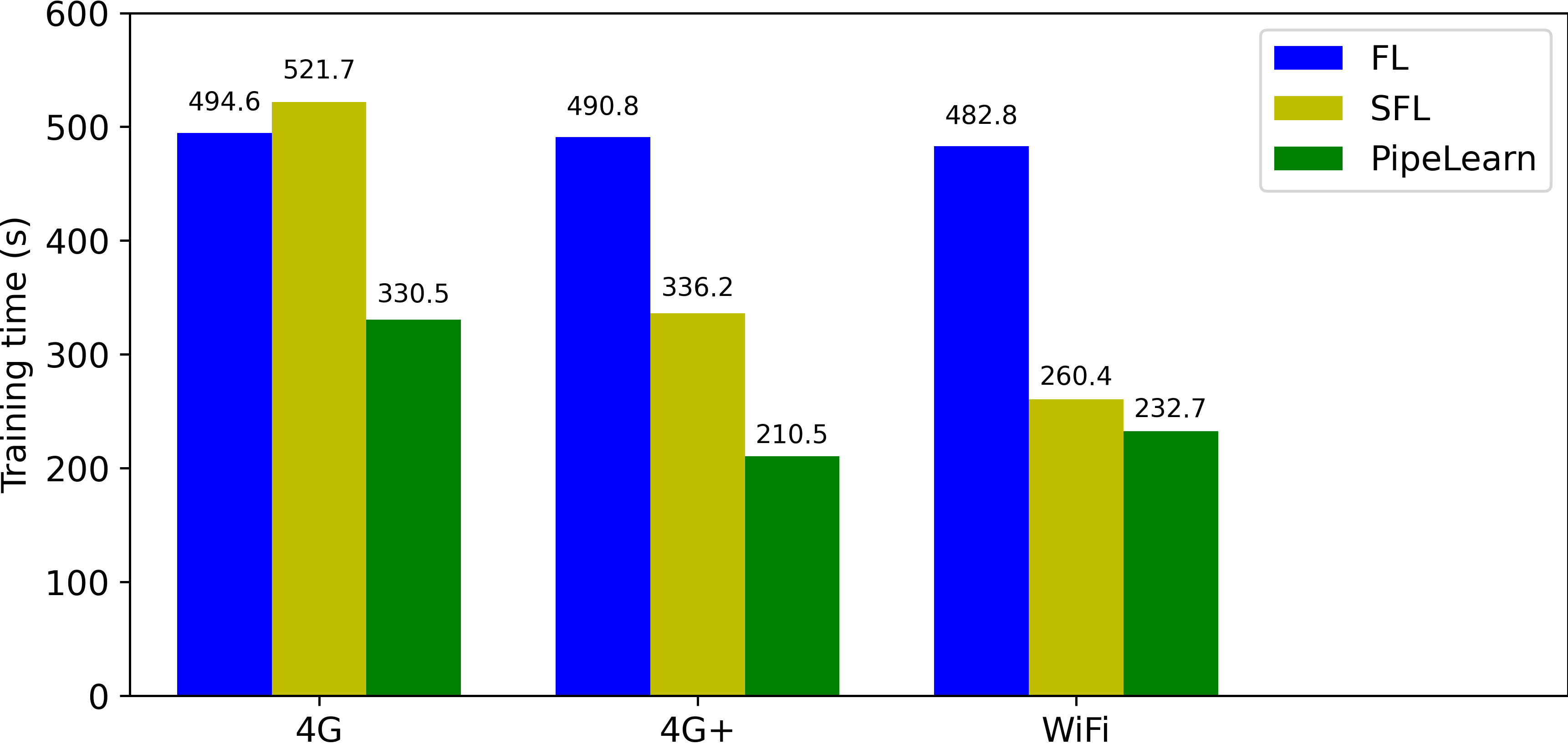
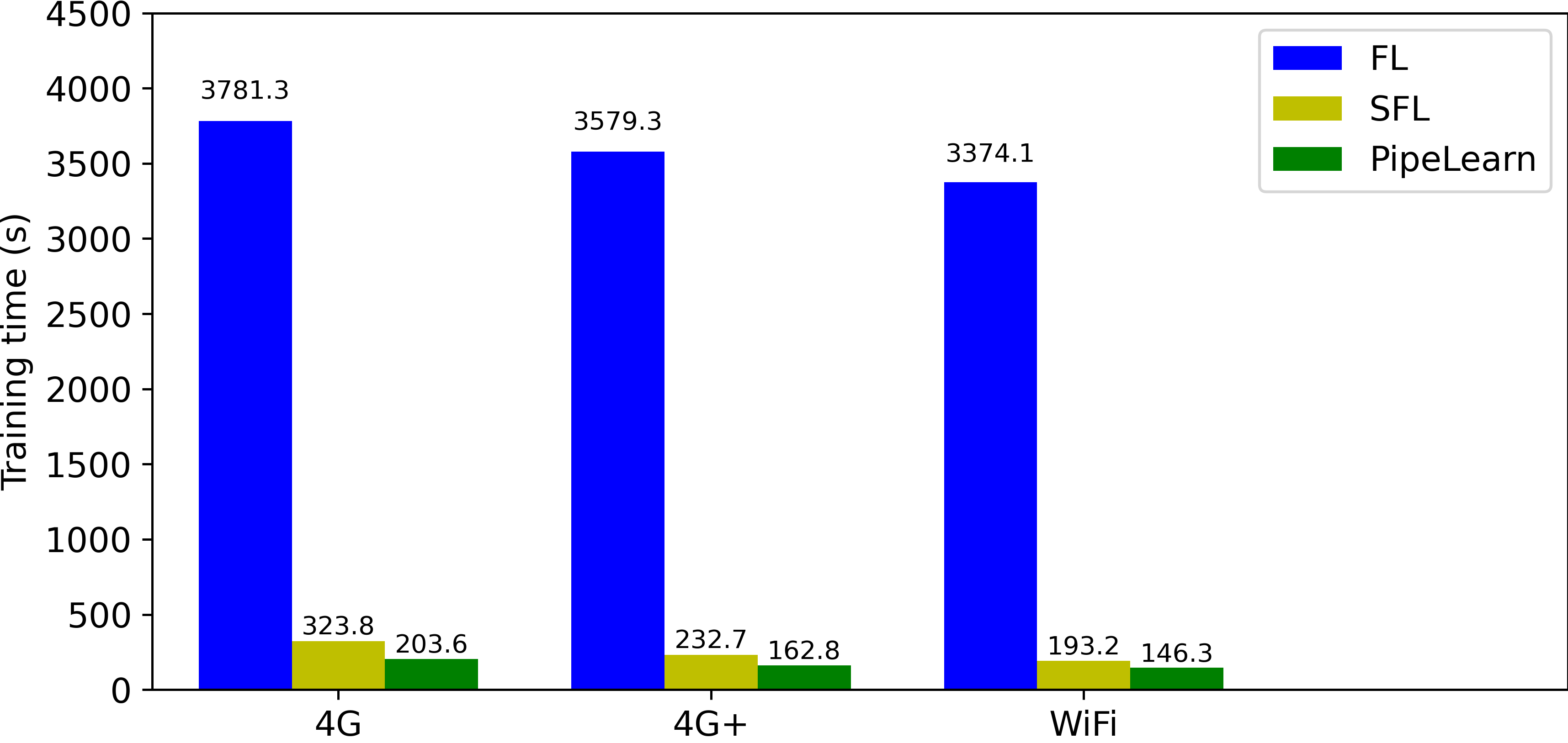
The efficiency of the CML techniques is measured by training time per epoch. Since a fixed number of images are trained in each training epoch, training time per epoch effectively captures the time taken by a CML technique to process one image.
Figure 4 shows the training time per epoch of VGG5 and ResNet18 for FL, SFL and PipeLearn under 4G, 4G+ and WiFi network conditions. It is immediately evident that the training time per epoch for PipeLearn is lower than FL and SFL in all cases.
When training VGG5 models (Figure 4(a)), FL requires similar time under three network conditions, because the devices only upload and download once at the end of the training epoch (it requires less communication compared to SFL and PipeLearn). However, FL trains the entire model on each device, which requires longer computational time. When the bandwidth is low (for example, 4G), FL outperforms SFL, because the latter requires more communication time. However, under 4G+ and WiFi, SFL has shorter training times because of fewer device-side computations. Under all network conditions, PipeLearn outperforms FL and SFL. It is noteworthy that the benefits of PipeLearn are evident when training needs to occur in a limited bandwidth environment since more computations can be overlapped with communication (communication takes more time under limited bandwidth). PipeLearn accelerates FL by 1.5x - 2.3x and SFL by 1.1x - 1.6x.
FL is slow when training ResNet18 (Figure 4(b)), because it is a deeper network with more layers that need to be trained on devices. Both of SFL and PipeLearn significantly outperform FL. PipeLearn has shortest training time per epoch under all network conditions. PipeLearn accelerates FL by 19.52x - 21.55x and SFL by 1.1x - 1.42x.
IV-B2 Comparing Resources Utilisation
Two metrics are used to compare the utilisation of hardware and bandwidth resources:
a) Idle time of server/device (seconds) is the time that the server/device does not contribute to training models in each training epoch. The device-side idle time is the average of idle time for all devices. Lower idle time means higher hardware resource utilisation. Since the devices are homogeneous, it is assumed that there is a negligible impact of stragglers.
b) Average network throughput (Mbps) is the average amount of data transmitted through the network per second when the model is trained. A higher network throughput means higher bandwidth resource utilisation.
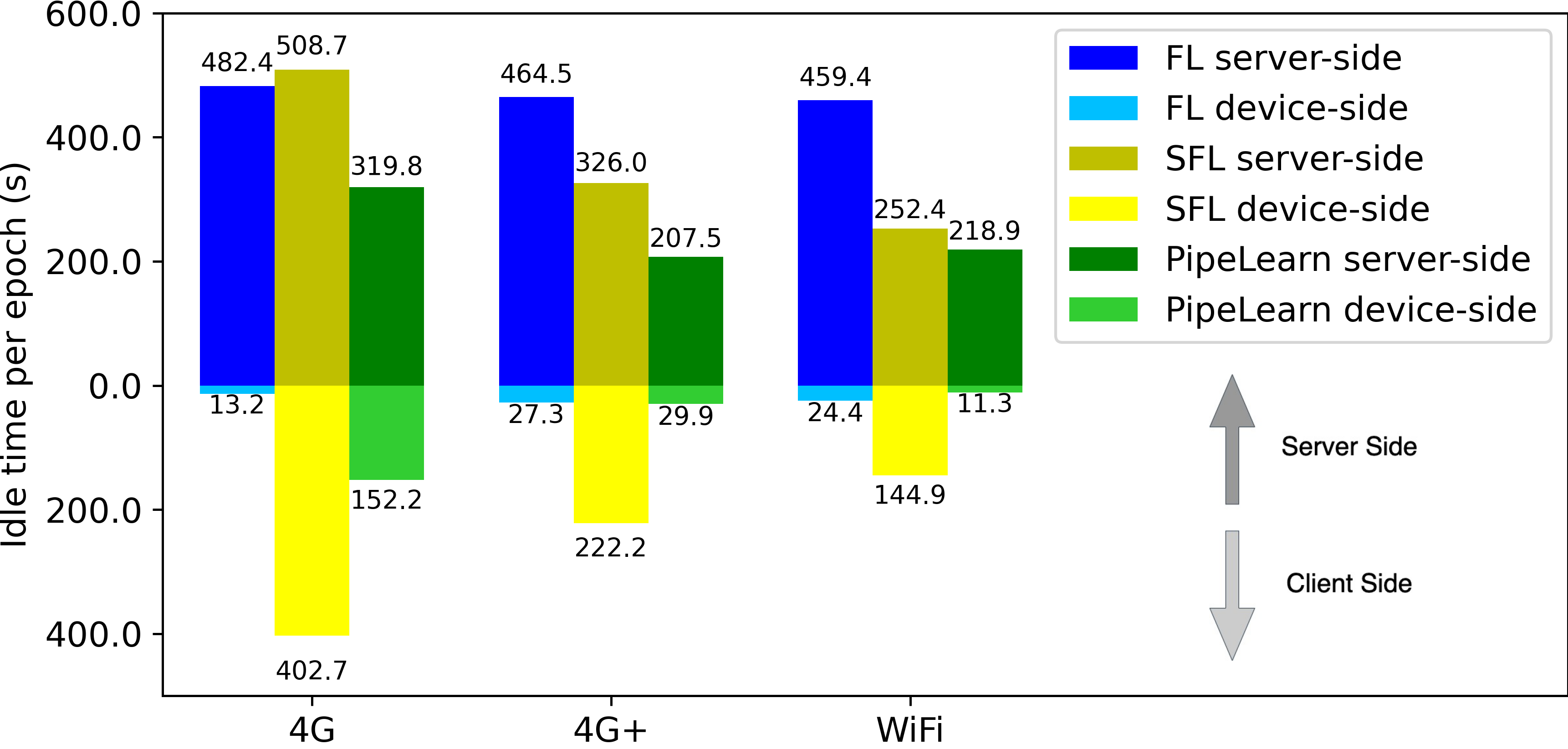
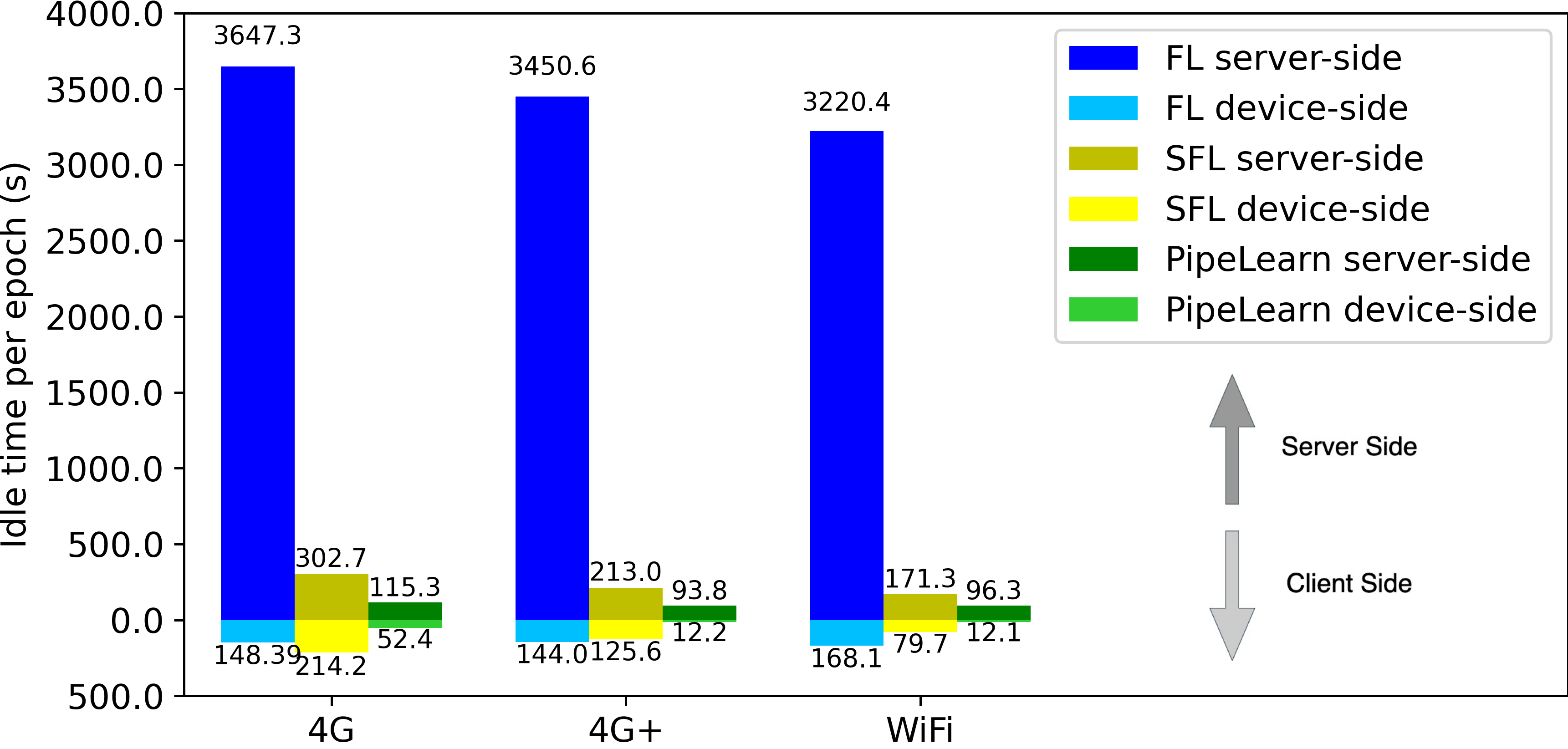
As shown in Figure 5, PipeLearn reduces the server-side idle time under all network conditions when training both VGG5 and ResNet18. Since the the server has more computing resources than the devices, model training is faster on the server. Hence, reducing the server-side idle time takes precedence over reducing the device-side idle time. Since FL trains complete models on the devices, the devices are usually rarely idle. However, the server is idle for a large proportion of time when the model is trained. Compared to FL, SFL utilises more resources on the server, because multiple layers are trained by the server. PipeLearn further reduces the server-side idle time by parallelising the server-side computation with device-side computation and communication between the server and the devices. Compared to FL and SFL, the server-side idle time using PipeLearnis reduced up to 28.5x and 1.81x, respectively. PipeLearn also reduces the device-side idle time of SFL upto 12.87x in all cases.
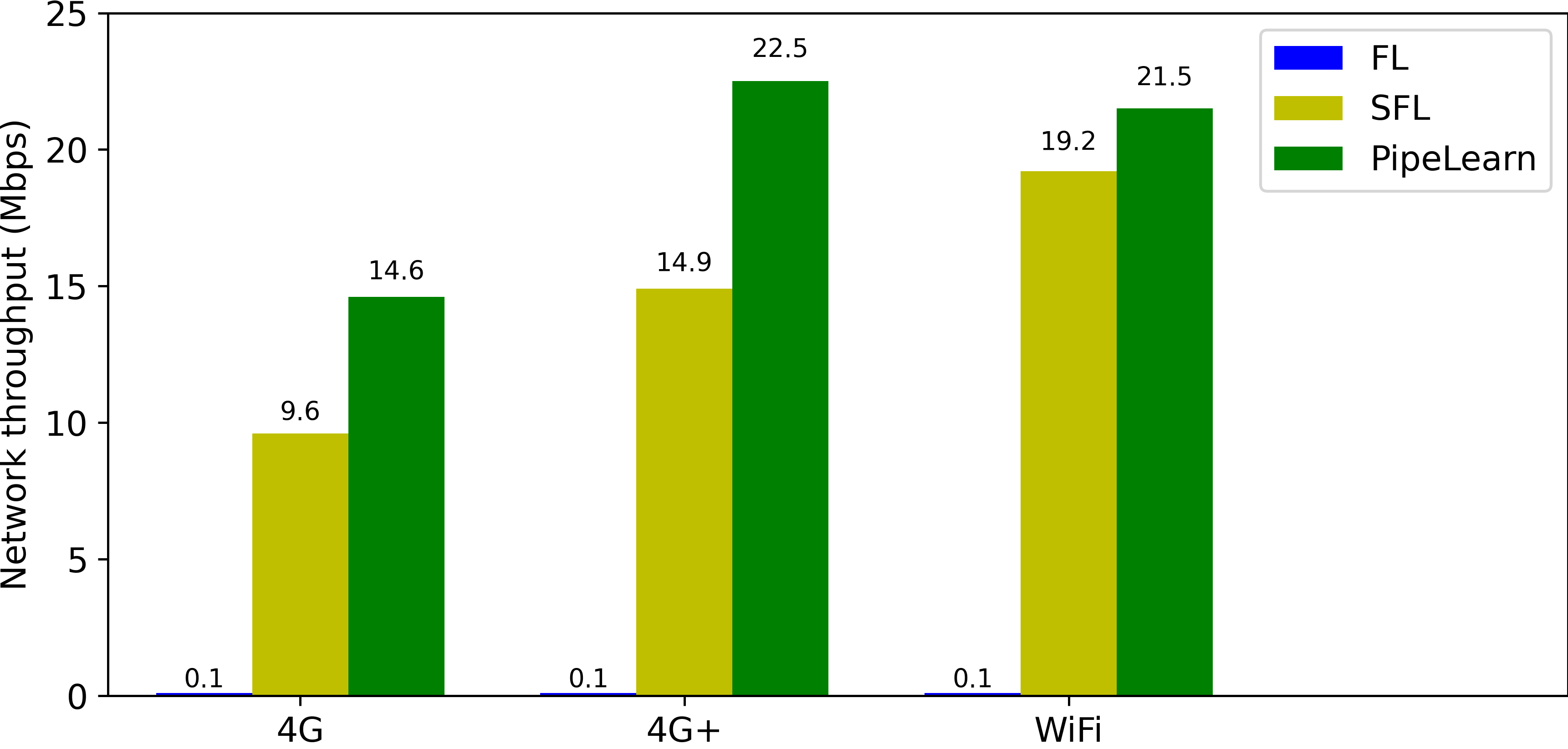
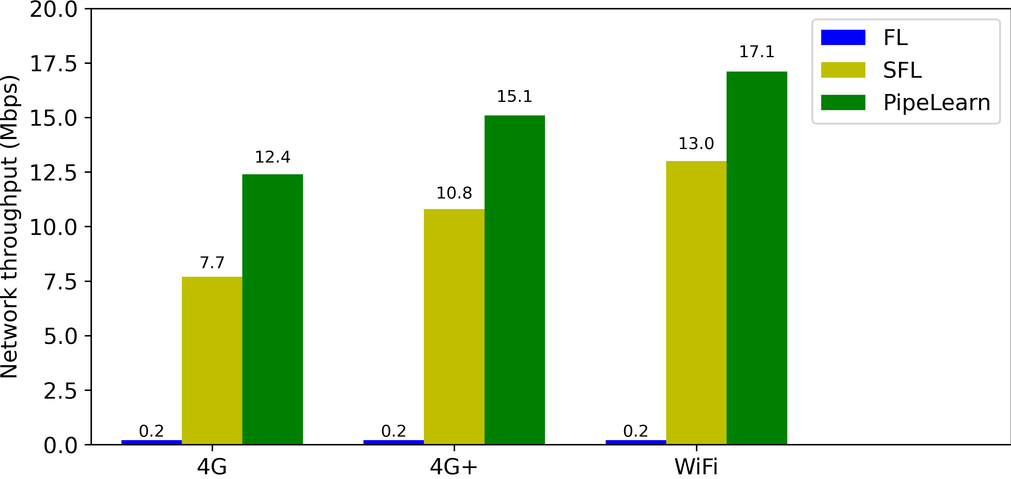
In terms of bandwidth utilisation (Figure 6), PipeLearn is more superior in performance than FL and SFL under all network conditions. FL has a low average network throughput, because communication is only required at the aggregation stage. A higher amount of data is transferred between the server and the devices in SFL than PipeLearn. However, by parallelising communication and computation, PipeLearn increases the network throughput by 321.29x and 1.52x compared to FL and SFL, respectively.
IV-C Model Accuracy and Convergence Results
It is theoretically proven in Section III that PipeLearn achieves similar model accuracy and convergence as FL. It is empirically demonstrated that PipeLearn does not adversely impact convergence and accuracy of models.
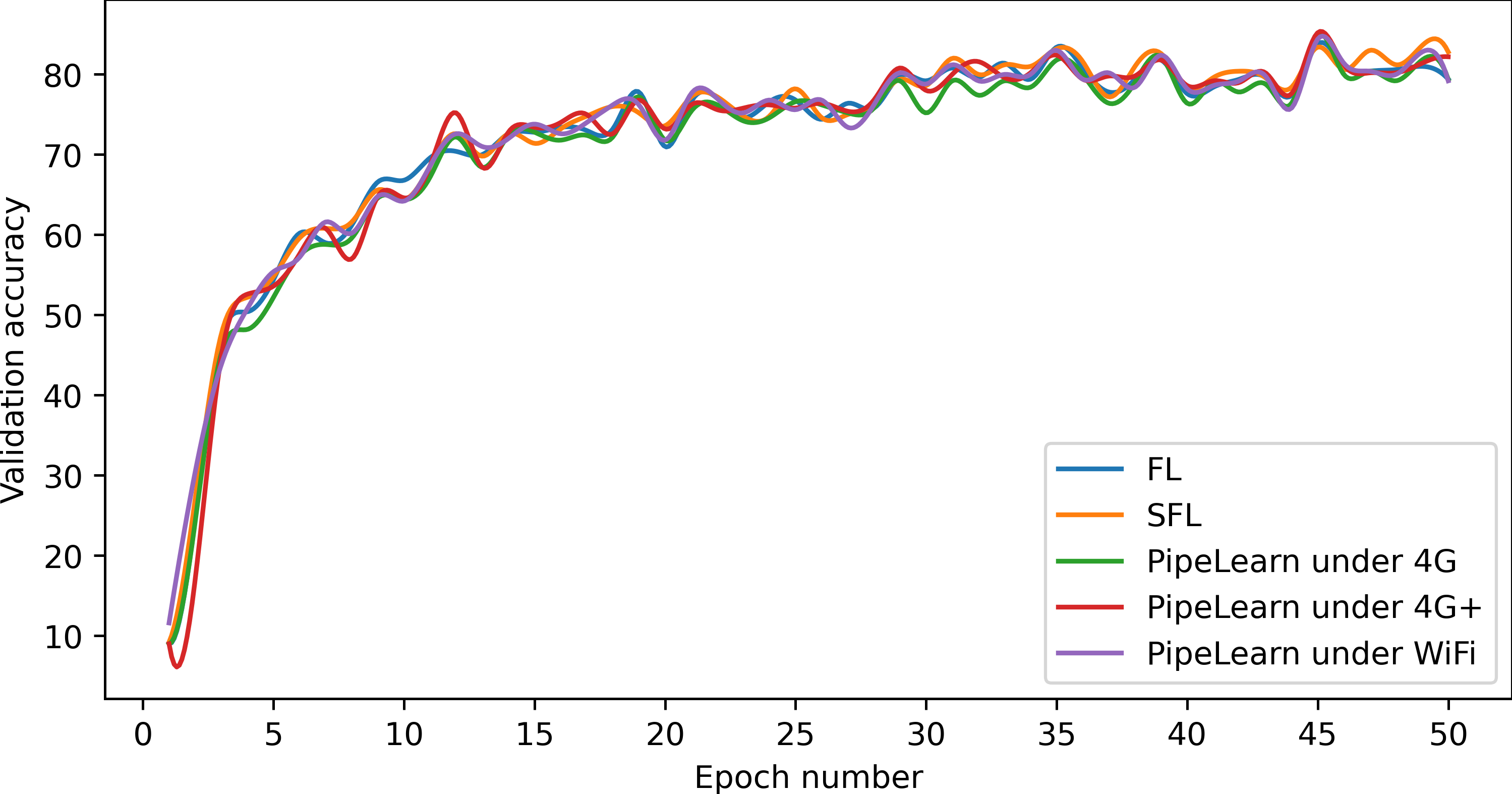
The convergence curves and test accuracy of VGG5 and ResNet18 using FL, SFL and PipeLearn are reported. Since the network conditions do not affect model convergence and accuracy in FL and SFL, the results for only 4G are reported. PipeLearn selects different split points and parallel batch numbers under different network conditions, so the results are reported for all network conditions.
IV-C1 Comparing Convergence
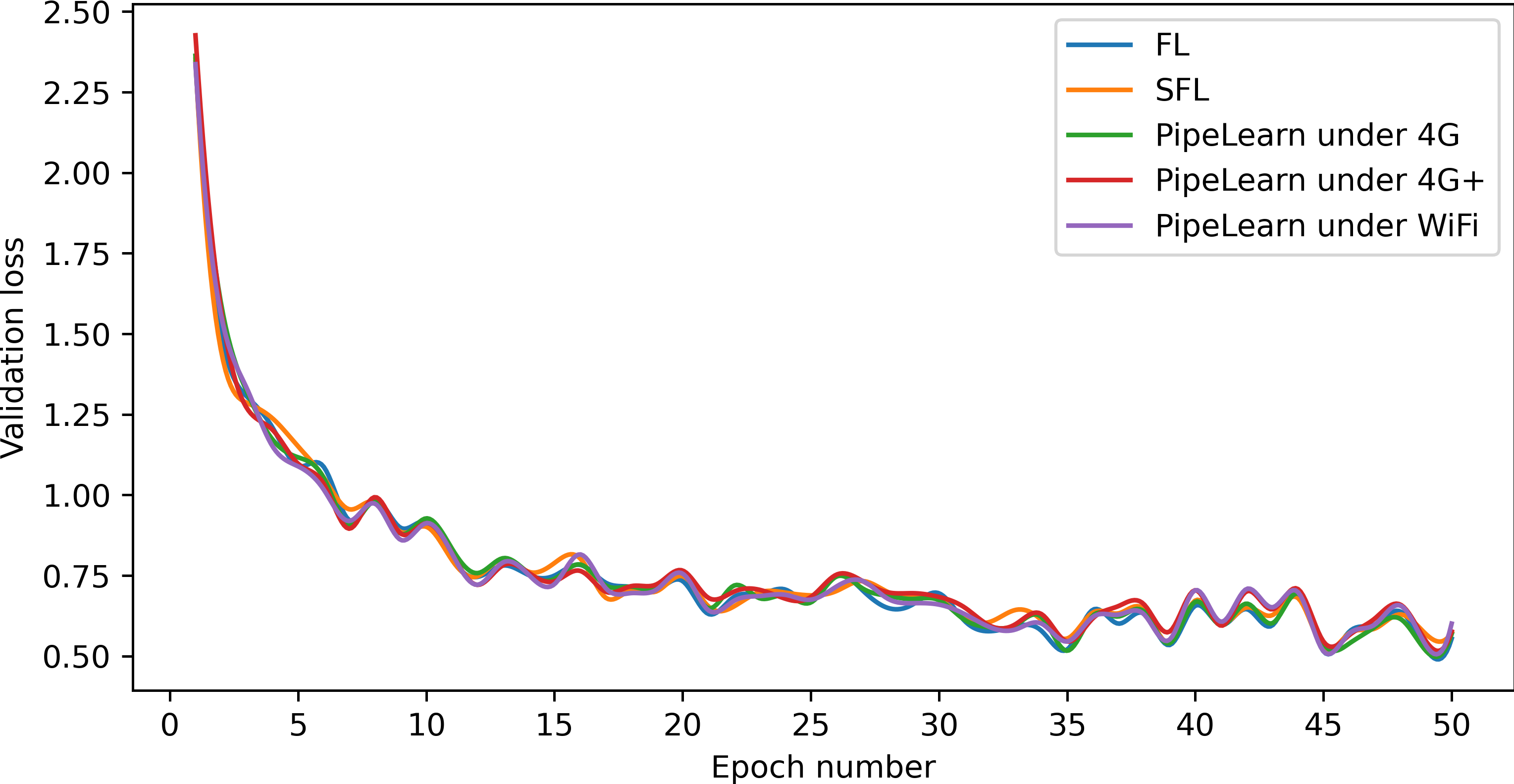
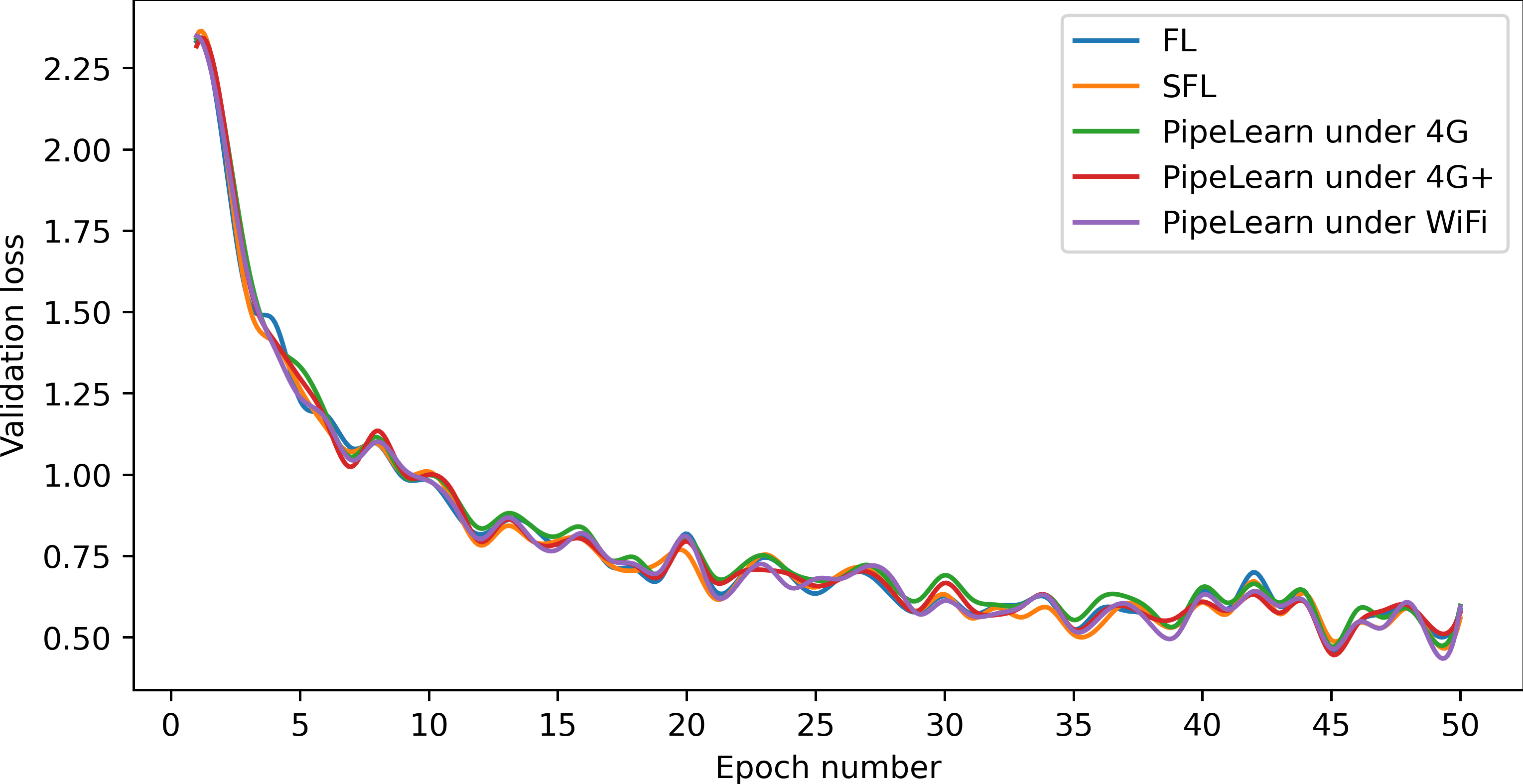
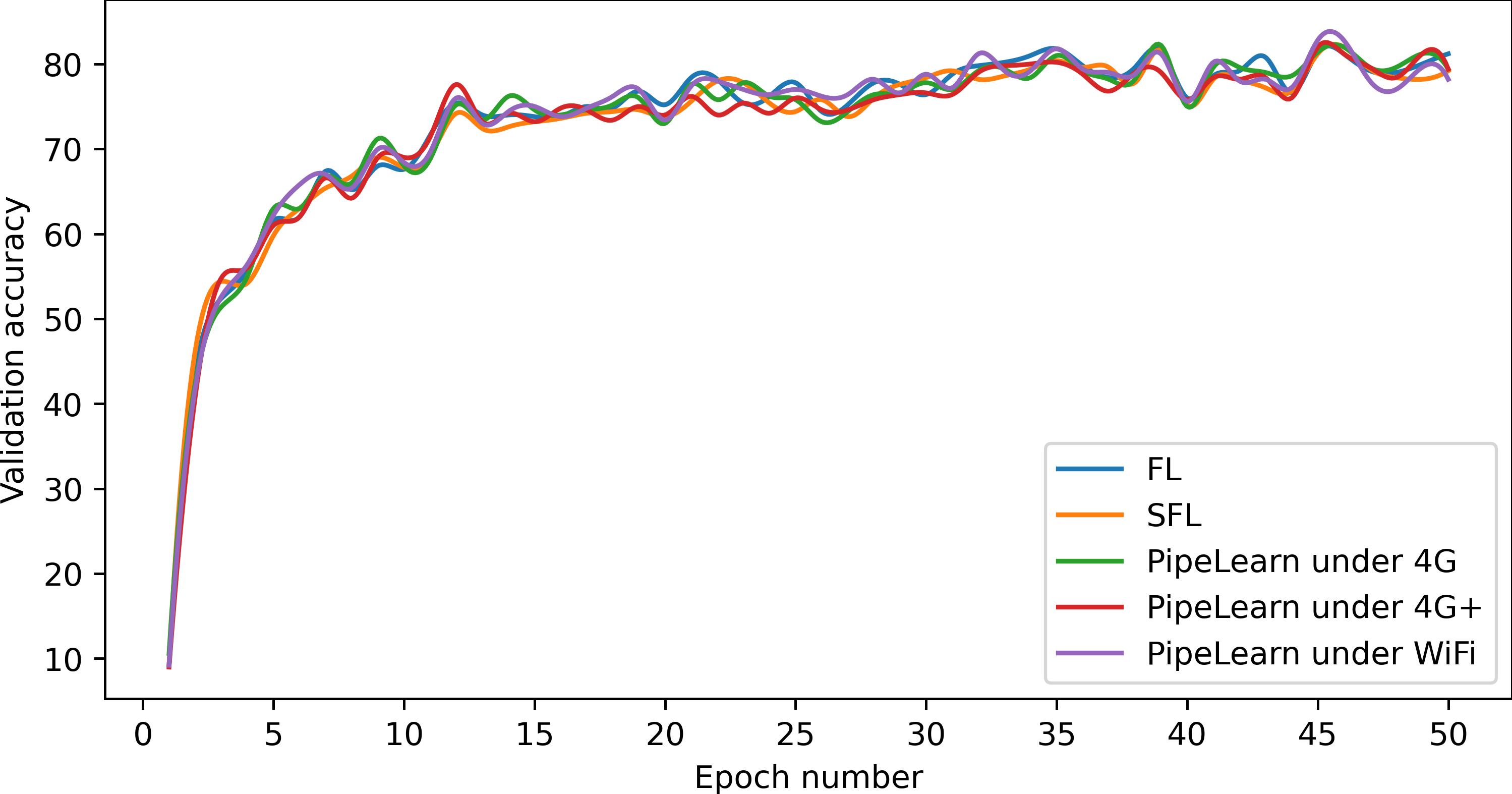
As shown in Figure 7, the loss curves of the five techniques on validation dataset have very similar trends for both VGG5 and ResNet18. Both VGG5 and ResNet18 converge within 50 epochs. Figure 8 shows that the five accuracy curves have significant overlap and demonstrate that PipeLearn does not impact model convergence.
IV-C2 Comparing Accuracy
In Table III, the test accuracy of VGG5 and ResNet18 trained using FL, SFL and PipeLearn under different network conditions are reported after 50 epochs. PipeLearn under three network conditions achieves a similar accuracy for both VGG5 and ResNet18 as FL and SFL on the test dataset. In short, PipeLearn does not sacrifice model accuracy.
| Model | Technique | Test Accuracy |
|---|---|---|
| VGG5 | FL | 79.95 |
| SFL | 79.55 | |
| PipeLearn under 4G | 79.15 | |
| PipeLearn under 4G+ | 78.4 | |
| PipeLearn under WiFi | 78.65 | |
| ResNet18 | FL | 80.4 |
| SFL | 81.55 | |
| PipeLearn under 4G | 79.5 | |
| PipeLearn under 4G+ | 81.35 | |
| PipeLearn under WiFi | 80.2 |
IV-D Optimisation Experiments
The results presented here are to demonstrate the effectiveness of the pipeline optimisation approach in PipeLearn. The experiments in this section will exhaustively benchmark all possible parameters, and prove that parameters selected by PipeLearn is similar to the optimal values for the parameters.
The control parameters of PipeLearn, namely the split point and parallel batch number for device , where , which affects the training efficiency were presented in Section III-C. Section IV-B demonstrated that PipeLearn with the parameters selected by our optimisation approach outperforms FL and SFL in terms of training efficiency.
The split point and parallel batch number for every device is the same as the experiments are carried out with homogeneous devices.
The number of split points are limited. As shown in Table II, VGG5 and ResNet18 consist of 5 and 10 sequential parameterised layers, respectively. Hence, we have for VGG5 and for ResNet18. The parallel batch numbers are also limited. As mentioned in Section IV-A, the batch size for PipeLearn is , where is the parallel batch number for homogeneous devices. To guarantee that the batch size is at least 1, we have . Due to the limited number of the split points and parallel batch numbers, the optimal pair is determined by exhaustive search. Specifically, VGG5 and ResNet18 are trained using all possible pairs in PipeLearn, and the pair with the shortest training time is considered optimal.
denotes the training time for each epoch given and . Equation 15 is used to score the selected parameters.
| (15) |
where . The higher the score the better. When the selected parameters are optimal, the score is 1.
The experimental results for the parameters selected by our approach and the optimal parameters are shown in Table IV. PipeLearn selects the optimal parameters in 4 out of 6 experiments. In only two experiments (VGG5 under WiFi and ResNet under 4G), the parameters selected by our approach are not the optimal ones. However, in these cases, our approach selects near-optimal split points, and their scores are closes to 1 (0.96 and 0.98).
| Model | Network | Selected Parameters | Optimal Parameters | Score of Selected Parameters | ||||
| Training Time | Training Time | |||||||
| VGG5 | 4G | 1 | 12 | 330.5 | 1 | 12 | 330.5 | 1 |
| 4G+ | 1 | 7 | 218.4 | 1 | 7 | 218.4 | 1 | |
| WiFi | 1 | 5 | 232.7 | 1 | 3 | 223.7 | 0.96 | |
| ResNet | 4G | 1 | 10 | 203.6 | 1 | 9 | 199.9 | 0.98 |
| 4G+ | 1 | 7 | 162.8 | 1 | 7 | 162.8 | 1 | |
| WiFi | 1 | 5 | 146.3 | 1 | 5 | 146.3 | 1 | |
It is worth noting that the optimal value of is always 1 under different conditions. This is because the devices have substantially less computing resources than the server. As a result, more layers are deployed on the server side. To explore whether PipeLearn finds the optimal parameters when , we fixed and search for using our approach. Figure 9 shows the scores of selected parameters given different values of under different network conditions. In most cases, the approach finds the optimal parameters (). Only three exceptions are noted; the selected parameters have high scores (from 0.93 to 0.98) although they are not optimal.
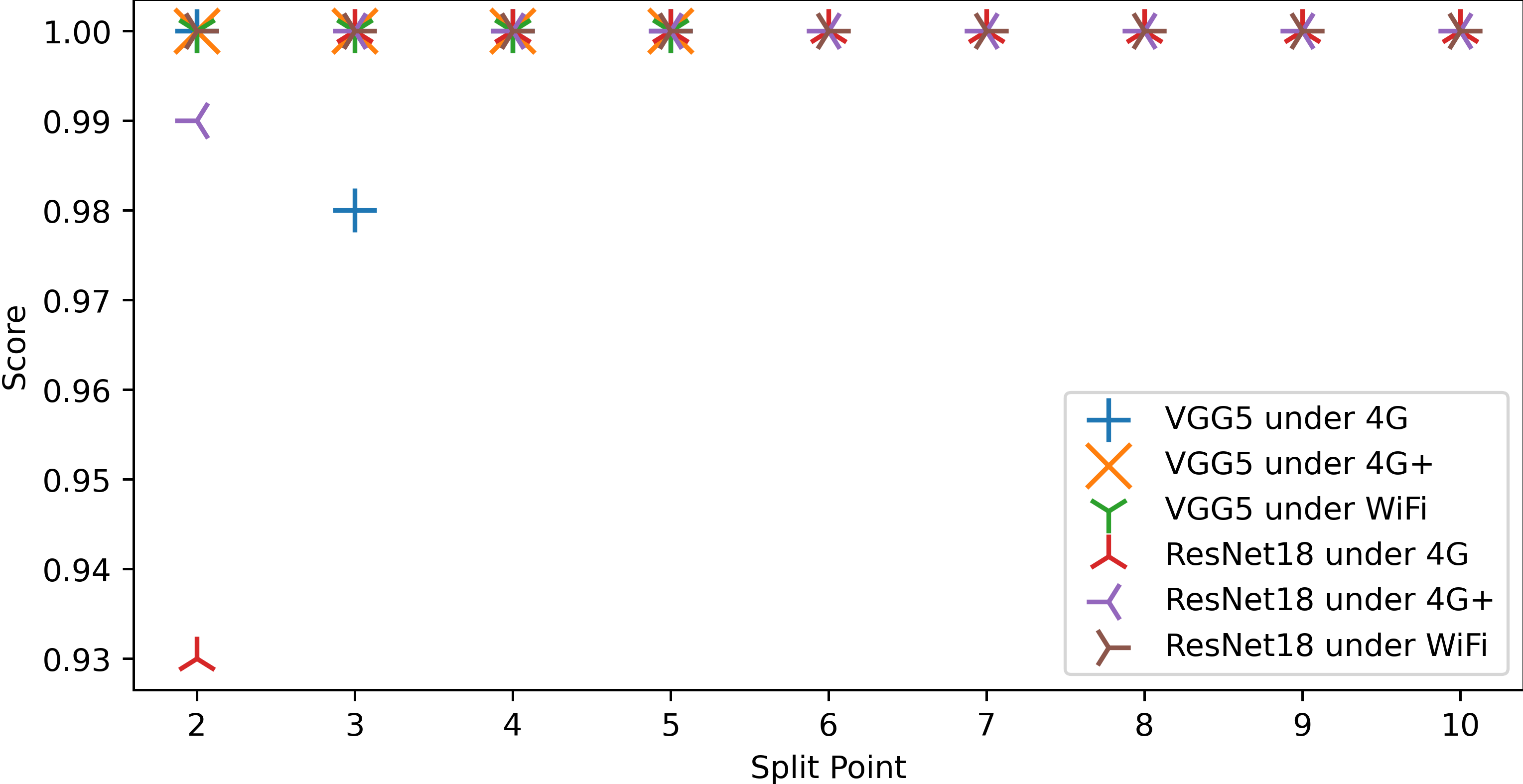
The experimental results highlight that the pipeline optimisation approach of PipeLearn is able to find the optimal or near-optimal parameters that maximise the training efficiency.
V Conclusion
Deep learning models are collaboratively trained using paradigms, such as federated learning, split learning or split federated learning on a server and multiple devices. However, they are limited in that the computation and communication across the server and devices is inherently sequential. This results in low compute and network resource utilisation and leads to idle time on the resources. We propose a novel framework, PipeLearn, that addresses this problem for the first time by taking advantage of pipeline parallelism, thereby accelerating the entire training process. A novel training pipeline is developed to parallelise server-side computation, device-side computation and server-device communication. In the training pipeline, the neural network is split and deployed on the server and devices, and the training process on different mini-batches of data is re-ordered. An optimisation approach is then proposed to maximise the resource utilisation of the pipeline by selecting control parameters. Consequently, when compared to existing paradigms, our pipeline significantly reduces idle time on compute resources by up to 28.5x and network resources by up to 321.3x in training popular convolutional neural networks under different network conditions. An overall training speed up of up to 21.6x is observed.
Acknowledgment
This work was sponsored by Rakuten Mobile, Inc., Japan.
References
- [1] A. Kendall and Y. Gal, “What Uncertainties Do We Need in Bayesian Deep Learning for Computer Vision?” in 31st International Conference on Neural Information Processing Systems, 2017, p. 5580–5590.
- [2] K. He, G. Gkioxari, P. Dollár, and R. Girshick, “Mask R-CNN,” in 2017 IEEE International Conference on Computer Vision, 2017, pp. 2980–2988.
- [3] J. Devlin, M.-W. Chang, K. Lee, and K. Toutanova, “BERT: Pre-training of Deep Bidirectional Transformers for Language Understanding,” in Conference of the North American Chapter of the Association for Computational Linguistics: Human Language Technologies, Volume 1 (Long and Short Papers), 2019, pp. 4171–4186.
- [4] T. Brown, B. Mann, N. Ryder, M. Subbiah, J. D. Kaplan, P. Dhariwal, A. Neelakantan, P. Shyam, G. Sastry, A. Askell, S. Agarwal, A. Herbert-Voss, G. Krueger, T. Henighan, R. Child, A. Ramesh, D. Ziegler, J. Wu, C. Winter, C. Hesse, M. Chen, E. Sigler, M. Litwin, S. Gray, B. Chess, J. Clark, C. Berner, S. McCandlish, A. Radford, I. Sutskever, and D. Amodei, “Language Models are Few-Shot Learners,” in Advances in Neural Information Processing Systems, vol. 33, 2020, pp. 1877–1901.
- [5] A. Graves, “Sequence Transduction with Recurrent Neural Networks,” CoRR, vol. abs/1211.3711, 2012.
- [6] A. Y. Hannun, C. Case, J. Casper, B. Catanzaro, G. Diamos, E. Elsen, R. Prenger, S. Satheesh, S. Sengupta, A. Coates, and A. Y. Ng, “Deep Speech: Scaling up End-to-End Speech Recognition,” CoRR, vol. abs/1412.5567, 2014.
- [7] C. Thapa, M. A. P. Chamikara, and S. A. Camtepe, Federated Learning Systems: Towards Next-Generation AI. Springer International Publishing, 2021, ch. Advancements of Federated Learning Towards Privacy Preservation: From Federated Learning to Split Learning, pp. 79–109.
- [8] J. Konečný, B. McMahan, and D. Ramage, “Federated optimization: Distributed optimization beyond the datacenter,” CoRR, vol. abs/1511.03575, 2015.
- [9] J. Konečný, H. B. McMahan, D. Ramage, and P. Richtárik, “Federated Optimization: Distributed Machine Learning for On-Device Intelligence,” CoRR, vol. abs/1610.02527, 2016.
- [10] J. Konečný, H. B. McMahan, F. X. Yu, P. Richtárik, A. T. Suresh, and D. Bacon, “Federated Learning: Strategies for Improving Communication Efficiency,” CoRR, vol. abs/1610.05492, 2016.
- [11] B. McMahan, E. Moore, D. Ramage, S. Hampson, and B. A. y. Arcas, “Communication-Efficient Learning of Deep Networks from Decentralized Data,” in 20th International Conference on Artificial Intelligence and Statistics, vol. 54. Proceedings of Machine Learning Research, 2017, pp. 1273–1282.
- [12] O. Gupta and R. Raskar, “Distributed Learning of Deep Neural Network over Multiple Agents,” CoRR, vol. abs/1810.06060, 2018.
- [13] P. Vepakomma, O. Gupta, T. Swedish, and R. Raskar, “Split Learning For Health: Distributed Deep Learning without Sharing Raw Patient Data,” CoRR, vol. abs/1812.00564, 2018.
- [14] C. Thapa, M. A. P. Chamikara, and S. Camtepe, “SplitFed: When Federated Learning Meets Split Learning,” CoRR, vol. abs/2004.12088, 2020.
- [15] D. Wu, R. Ullah, P. Harvey, P. Kilpatrick, I. Spence, and B. Varghese, “FedAdapt: Adaptive Offloading for IoT Devices in Federated Learning,” IEEE Internet of Things Journal, vol. 9, no. 21, pp. 20 889–20 901, 2022.
- [16] Z. Ji, L. Chen, N. Zhao, Y. Chen, G. Wei, and F. R. Yu, “Computation Offloading for Edge-Assisted Federated Learning,” IEEE Transactions on Vehicular Technology, vol. 70, no. 9, pp. 9330–9344, 2021.
- [17] Y. Ye, S. Li, F. Liu, Y. Tang, and W. Hu, “EdgeFed: Optimized Federated Learning Based on Edge Computing,” IEEE Access, vol. 8, pp. 209 191–209 198, 2020.
- [18] X. Chen, J. Li, and C. Chakrabarti, “Communication and Computation Reduction for Split Learning using Asynchronous Training,” CoRR, vol. abs/2107.09786, 2021.
- [19] A. Singh, P. Vepakomma, O. Gupta, and R. Raskar, “Detailed Comparison of Communication Efficiency of Split Learning and Federated Learning,” CoRR, vol. abs/1909.09145, 2019.
- [20] Y. Gao, M. Kim, S. Abuadbba, Y. Kim, C. Thapa, K. Kim, S. A. Camtep, H. Kim, and S. Nepal, “End-to-End Evaluation of Federated Learning and Split Learning for Internet of Things,” in International Symposium on Reliable Distributed Systems, 2020, pp. 91–100.
- [21] H. Yuan and T. Ma, “Federated Accelerated Stochastic Gradient Descent,” in Advances in Neural Information Processing Systems, vol. 33, 2020, pp. 5332–5344. [Online]. Available: https://proceedings.neurips.cc/paper/2020/file/39d0a8908fbe6c18039ea8227f827023-Paper.pdf
- [22] C. Xu, Z. Hong, M. Huang, and T. Jiang, “Acceleration of Federated Learning with Alleviated Forgetting in Local Training,” in International Conference on Learning Representations, 2022. [Online]. Available: https://openreview.net/forum?id=541PxiEKN3F
- [23] W. Liu, L. Chen, Y. Chen, and W. Zhang, “Accelerating Federated Learning via Momentum Gradient Descent,” IEEE Transactions on Parallel and Distributed Systems, vol. 31, no. 8, pp. 1754–1766, 2020.
- [24] H. Wu and P. Wang, “Fast-Convergent Federated Learning with Adaptive Weighting,” CoRR, vol. abs/2012.00661, 2020.
- [25] Y. Wang, J. Wolfrath, N. Sreekumar, D. Kumar, and A. Chandra, “Accelerated Training via Device Similarity in Federated Learning,” in Proceedings of the 4th International Workshop on Edge Systems, Analytics and Networking, 2021, p. 31–36.
- [26] H. Wang, Z. Kaplan, D. Niu, and B. Li, “Optimizing Federated Learning on Non-IID Data with Reinforcement Learning,” in IEEE Conference on Computer Communications, 2020, pp. 1698–1707.
- [27] T. Nishio and R. Yonetani, “Client Selection for Federated Learning with Heterogeneous Resources in Mobile Edge,” CoRR, vol. abs/1804.08333, 2018.
- [28] Z. Xu, F. Yu, J. Xiong, and X. Chen, “Helios: Heterogeneity-Aware Federated Learning with Dynamically Balanced Collaboration,” in 2021 58th ACM/IEEE Design Automation Conference (DAC), 2021, pp. 997–1002.
- [29] Z. Wang, H. Xu, J. Liu, Y. Xu, H. Huang, and Y. Zhao, “Accelerating Federated Learning with Cluster Construction and Hierarchical Aggregation,” IEEE Transactions on Mobile Computing, 2022.
- [30] Z. Qu, S. Guo, H. Wang, B. Ye, Y. Wang, A. Zomaya, and B. Tang, “Partial Synchronization to Accelerate Federated Learning over Relay-Assisted Edge Networks,” IEEE Transactions on Mobile Computing, 2021.
- [31] W. Xu, W. Fang, Y. Ding, M. Zou, and N. Xiong, “Accelerating Federated Learning for IoT in Big Data Analytics With Pruning, Quantization and Selective Updating,” IEEE Access, vol. 9, pp. 38 457–38 466, 2021.
- [32] S. Pal, M. Uniyal, J. Park, P. Vepakomma, R. Raskar, M. Bennis, M. Jeon, and J. Choi, “Server-Side Local Gradient Averaging and Learning Rate Acceleration for Scalable Split Learning,” CoRR, vol. abs/2112.05929, 2021.
- [33] Y. Huang, Y. Cheng, A. Bapna, O. Firat, D. Chen, M. Chen, H. Lee, J. Ngiam, Q. V. Le, Y. Wu, and z. Chen, “GPipe: Efficient Training of Giant Neural Networks using Pipeline Parallelism,” in Advances in Neural Information Processing Systems, H. Wallach, H. Larochelle, A. Beygelzimer, F. d'Alché-Buc, E. Fox, and R. Garnett, Eds., vol. 32, 2019.
- [34] D. Narayanan, A. Harlap, A. Phanishayee, V. Seshadri, N. R. Devanur, G. R. Ganger, P. B. Gibbons, and M. Zaharia, “PipeDream: Generalized Pipeline Parallelism for DNN Training,” in Proceedings of the 27th ACM Symposium on Operating Systems Principles, T. Brecht and C. Williamson, Eds., 2019, pp. 1–15.
- [35] Y. Zhou, Q. Ye, and J. Lv, “Communication-Efficient Federated Learning With Compensated Overlap-FedAvg,” IEEE Transactions on Parallel and Distributed Systems, vol. 33, no. 1, p. 192–205, 2022.
- [36] K. Simonyan and A. Zisserman, “Very Deep Convolutional Networks for Large-scale Image Recognition,” arXiv preprint arXiv:1409.1556, 2014.
- [37] K. He, X. Zhang, S. Ren, and J. Sun, “Deep Residual Learning for Image Recognition,” CoRR, vol. abs/1512.03385, 2015.
- [38] A. Krizhevsky, V. Nair, and G. Hinton, “CIFAR-10 (Canadian Institute for Advanced Research),” 2009. [Online]. Available: http://www.cs.toronto.edu/~kriz/cifar.html
- [39] A. Krizhevsky and G. Hinton, “Learning Multiple Layers of Features from Tiny Images,” Master’s thesis, Department of Computer Science, University of Toronto, 2009.
- [40] L. Lockhart, P. Harvey, P. Imai, P. Willis, and B. Varghese, “Scission: Performance-driven and Context-aware Cloud-Edge Distribution of Deep Neural Networks,” in IEEE/ACM 13th International Conference on Utility and Cloud Computing, 2020, pp. 257–268.
Appendix A
It is proved here that splitting a neural network maintains the consistency of the training process and does not impact model accuracy. Assuming that is a mini-batch of data and is the corresponding label set, denotes the forward pass function of layer and denotes the output of layer , where .
| (16) |
The forward pass of the complete model in FL is:
| (17) |
where is the output of the final layer. If the model is split, the training process is split into two phases that happens on device side and server side, respectively.
| (18) |
| (19) |
where is the activations that transmitted from device to the server is the final output.
| (20) |
Thus, the loss function with and without splitting the model is also consistent.
| (21) |
We use to denote the backward pass function of layer q, which is the derivative of .
| (22) |
The weights in layer of the original model and the split model are denoted as and , respectively. Assume is the gradient function, then:
| (23) |
| (24) |
Since splitting neural network does not change the gradients, it does not influence the model accuracy.
Appendix B
It is proved here that the model accuracy remains the same before and after reordering the training stages. The dataset on client is denoted as . denotes a mini-batch in the original training process and , where , to denote mini-batches in a training round after reordering training stages, where .
In the original training process, the model is updated after the backward pass of each mini-batch . Assuming is the original model and is the learning rate, the updated model is:
| (26) |
In PipeLearn, the model is updated after the backward pass of the last mini-batch in each training round. The updated model is:
| (27) |
We have:
| (28) |
Therefore, the updated models with and without reordering the training stages are almost the same (exactly the same if ). Thus, reordering training stages does not affect the model accuracy.