Stochastic Generative Flow Networks
Abstract
Generative Flow Networks (or GFlowNets for short) are a family of probabilistic agents that learn to sample complex combinatorial structures through the lens of “inference as control”. They have shown great potential in generating high-quality and diverse candidates from a given energy landscape. However, existing GFlowNets can be applied only to deterministic environments, and fail in more general tasks with stochastic dynamics, which can limit their applicability. To overcome this challenge, this paper introduces Stochastic GFlowNets, a new algorithm that extends GFlowNets to stochastic environments. By decomposing state transitions into two steps, Stochastic GFlowNets isolate environmental stochasticity and learn a dynamics model to capture it. Extensive experimental results demonstrate that Stochastic GFlowNets offer significant advantages over standard GFlowNets as well as MCMC- and RL-based approaches, on a variety of standard benchmarks with stochastic dynamics.
1 Introduction
Recently, Generative Flow Networks [GFlowNets; Bengio et al., 2021a, b] have been successfully applied to a wide variety of tasks, including molecule discovery [Bengio et al., 2021a, Jain et al., 2022b], biological sequence design [Jain et al., 2022a], and robust scheduling [Zhang et al., 2023a]. GFlowNets learn policies to generate objects sequentially, and are related to Monte-Carlo Markov chain (MCMC) methods [Metropolis et al., 1953, Hastings, 1970, Andrieu et al., 2003], generative models [Goodfellow et al., 2014, Ho et al., 2020], and amortized variational inference [Kingma and Welling, 2013]. The sequential process of generating an object following a policy bears a close resemblance to reinforcement learning [RL; Sutton and Barto, 2018]. Contrary to the typical reward-maximizing policy in RL [Mnih et al., 2015, Lillicrap et al., 2015, Haarnoja et al., 2017, Fujimoto et al., 2018, Haarnoja et al., 2018], GFlowNets aim to learn a stochastic policy for sampling composite objects with probability proportional to the reward function . This is desirable in many real-world tasks where the diversity of solutions is important, and we aim to sample a diverse set of high-reward candidates, including recommender systems [Kunaver and Požrl, 2017], drug discovery [Bengio et al., 2021a, Jain et al., 2022a], and sampling causal models from a Bayesian posterior [Deleu et al., 2022], among others.

Existing work on GFlowNets [Bengio et al., 2021a, Malkin et al., 2022a, Madan et al., 2022], however, is limited to deterministic environments, where state transitions are deterministic, which may limit their applicability in the more general stochastic cases in practice. Figure 1 illustrates an example with stochastic transition dynamics where existing GFlowNet approaches can fail. Standard GFlowNet approaches will result in and when trained to completion (with denoting the probability of sampling state ), which does not match the ideal case where and . Therefore, the learned policy does not sample proportionally to the reward function in the presence of stochastic transition dynamics. In practice, many tasks involve stochasticity in state transitions, which are more challenging to solve but are applicable to a wide variety of problems [Antonoglou et al., 2021, Yang et al., 2022, Paster et al., 2022].
To address this limitation, in this paper, we introduce a novel methodology, Stochastic GFlowNet, which is the first empirically effective approach for tackling environments with stochastic transition dynamics with GFlowNets. Stochastic GFlowNet decomposes the state transitions based on the concept of afterstates [Sutton and Barto, 2018, Bengio et al., 2021b]. Specifically, each stochastic state transition is decomposed into a deterministic step that transitions from the environment state to an intermediate state and a stochastic step that branches from the intermediate state to the next state . We propose a practical way for training the dynamics model to capture the stochastic environment dynamics. The methodology is general and can be applied to different GFlowNet learning objectives. The code is publicly available at https://github.com/ling-pan/Stochastic-GFN.
In summary, the contribution of this work is as follows:
-
•
We propose a novel method, Stochastic GFlowNet, which is the first empirically effective approach extending GFlowNets to the more general stochastic environments based on Bengio et al. [2021b].
-
•
We conduct extensive experiments on GFlowNet benchmark tasks augmented with stochastic transition dynamics, and validate the effectiveness of our approach in tackling stochastic environments. Results show that our method significantly outperforms existing baselines and scales well to the more complex and challenging biological sequence generation tasks.
2 Background
2.1 GFlowNet Preliminaries
We denote a directed acyclic graph (DAG) by , with the set of vertices corresponding to the states and the set of edges, which corresponds to the set of actions. There is a unique initial state which has no parent state; on the other hand, we define all states without children to be terminal states, whose set is denoted by . A GFlowNet learns stochastic policy which aims to sample complete trajectories where and to sample terminal states. Each trajectory is assigned a non-negative flow . A trajectory can be generated sequentially by sampling iteratively from the forward policy , which is a collection of distributions over the children at each state. Existing work on GFlowNets assumes a one-to-one correspondence between action and next state, making the definition of forward policy to be consistent to the notion of policy in general RL. Nonetheless, in this work, we relax this assumption and generalize GFlowNets to more flexible stochastic environments. The objective of GFlowNet learning is to sample terminal states with probability proportional to a given non-negative reward function for all . This indicates that all the flows that end up with should sum up to , namely , where is a trajectory that ends in and the sum is thus over all complete trajectories that lead to terminal state . To formalize this, we first define the terminating probability to be the marginal likelihood of sampling trajectories terminating at a terminal state :
| (1) |
Therefore, the goal of GFlowNet learning is to obtain a policy such that .
2.2 Learning Objectives for GFlowNets
In applicative tasks, practitioners need to design the GFlowNet modules (e.g., policies, flows) with parameterized neural networks, and further choose a training criterion to train these networks. In this subsection, we briefly summarize some learning criteria of GFlowNets.
Detailed balance (DB).
By summing the flows of all the trajectories going through a state , we can define a state flow . Such a function can be learned, together with forward and backward policy , where is a child state of . The backward policy , a collection of distributions over the parents of each state, is not part of the generative process, but serves as a tool for learning the forward policy . The GFlowNet detailed balance (DB) constraint is defined as
| (2) |
It is also worth noting that at terminal states , it pushes the flow at to match the terminal rewards . In practice, we transform the DB constraint into a training objective by setting the loss function to be a squared difference between the logarithm of the left and right-hand sides Bengio et al. [2021a] of Eq. (2). If the optimization objective is perfectly minimized, it would make the above flow consistency constraint satisfied, thus making the forward policy sample proportionally to given reward values, as desired. It means that after training, the constraint is only approximately achieved (and in general it would be intractable to obtain an exact solution).
Trajectory balance (TB).
In analogy to the forward decomposition of a complete trajectory in Eq. (1), we could use to represent the trajectory backward probability. As an alternative to DB, Malkin et al. [2022a] propose the trajectory balance (TB) criterion which operates on complete trajctories, instead of state transitions, defined as follows
| (3) |
where is any complete trajectory and is a learned scalar parameter, denoting the partition function of the reward distribution. Note that TB does not explicitly learn a flow function.
For on-policy training, we can simply use trajectories sampled from the forward policy to evaluate the training loss and its gradient with respect to the parameters of the neural networks. The GFlowNet training objectives can be further improved with off-policy training, i.e., with trajectories sampled from a broader and more exploratory distribution than [Malkin et al., 2022b]. A popular choice is using a tempered version of the current forward policy [Zhang et al., 2022b] or a mixture of the forward policy and a uniform random policy [Bengio et al., 2021a] that mimics -greedy exploration in RL.
3 Stochastic GFlowNets
We now describe the Stochastic GFlowNet, a novel method that learns a model of the environment to capture the stochasticity of state transitions. We first describe a key idea introduced by Bengio et al. [2021b] to decompose the GFlowNet transitions as per Figure 2, and then introduce a new approach to learn the GFlowNet policy and the dynamics model. We also discuss the applicability to different GFlowNet learning objectives and the resulting effects.
3.1 Proposed Method
Existing work on GFlowNets [Bengio et al., 2021a, Malkin et al., 2022a] typically makes the assumption that all transitions from a state to the next state within a trajectory are defined deterministically based on the selected action (and also there is only one action that can transition from to , with denoting the deterministic transition function). This applies to problems where the generative process for the objects is deterministic, which is appropriate when the actions are internal, e.g., choosing what to attend, what to imagine (such as solutions to problems), how to make inferences, etc. Yet, a number of real-world tasks are stochastic, either inherently or due to the environment complexity [Antonoglou et al., 2021, Paster et al., 2022, Yang et al., 2022]. In the more general stochastic environments, the action at can land in several possible next states. For instance, synthesizing proteins with oligo pools can result in the generation of variants of the specified protein [Song et al., 2021].
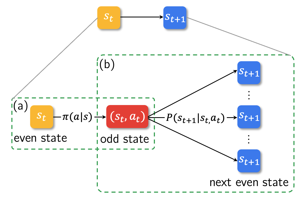
To cope with stochasticity in the transition dynamics, we decompose state transitions based on the concept of afterstates [Sutton and Barto, 2018, Bengio et al., 2021b]. Specifically, for a transition from a state to the next state , we decompose the transition in two steps. First, as illustrated in part (a) in Figure 2, we sample an action based on a policy in the current state (called an even state), and transit deterministically to an intermediate state , called an odd state. The flow consistency constraint for detailed balance (DB) for even-to-add transitions is shown in Eq. (4), since the backward policy probability is here (we can only get to from ):
| (4) |
The odd state can be considered as a hypothetical state after we apply an action before the environment gets involved [Antonoglou et al., 2021]. The environment dynamics then transform into to the next even state stochastically according to a distribution , which is the state transition function. This second step corresponds to part (b) in Figure 2, and the corresponding flow consistency constraint is
| (5) |
Note that an odd state can lead to many possible next even states due to stochasticity in the environment. With the introduction of odd states, we isolate the effect of choosing the action to apply in the environment and of the stochastic state transition given an action, with a deterministic and a stochastic step.
Training a Stochastic GFlowNet.
Combining the two steps, we obtain a novel flow consistency constraint which we call stochastic GFlowNets based on detailed balance (DB), where denotes the state transition function:
| (6) |
In practice, for training stochastic GFlowNets, we would minimize the loss in Eq. (7) based on the flow consistency constraint from Eq. (6), which is trained on a log-scale.
| (7) |
Note that our proposed methodology is general and can be applied to other GFlowNet learning objectives such as trajectory balance (TB), as we discuss in Section 3.2.
Learning the dynamics model.
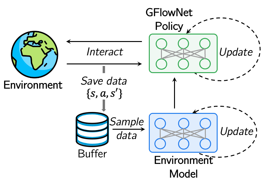
Since the transition dynamics are unknown in general, we need to learn it. In practice, we learn a model with parameters to approximate through maximum likelihood estimation (other techniques from generative and dynamics modeling [Venkatraman et al., 2015] could also be applied). We optimize its parameters with the interaction data using the Adam optimizer [Kingma and Ba, 2015] based on the loss function in Eq. (8), where the output of is a softmax distribution across all possible next states. The data is sampled from a experience replay buffer, which stores interaction data from the GFlowNet policy and the environment.
| (8) |
Practical implementation.
Figure 3 illustrates the major components of Stochastic GFlowNets as described above and how they interact with each other. The procedure for training Stochastic GFlowNet based on DB is summarized in Algorithm 1.
3.2 Discussion on the Applicability to Trajectory Balance (TB)
As discussed in Section 3.1, our proposed method is versatile and can be applied to other GFlowNet learning objectives beyond DB. We state the flow consistency constraint for Stochastic TB in Eq. (9), which is obtained via a telescoping calculation based on Eq. (6).
| (9) |
In practice, we can train with Stochastic TB by minimizing the loss obtained from Eq (9), i.e.,
| (10) |
However, as TB is optimized based on a sampled trajectory instead of each transition, it can lead to a larger variance as studied in Madan et al. [2022] even in deterministic environments. This problem can be further exacerbated in stochastic environments. In Section 4.1.3, we find that the Stochastic TB underperforms relative to Stochastic DB, presumable due to a larger variance, as studied by Madan et al. [2022].
4 Experiments
In this section, we conduct extensive experiments to investigate the following key questions: i) How much can Stochastic GFNs improve over GFNs in the presence of stochastic transition dynamics? ii) Can Stochastic GFNs be built upon different GFlowNets learning objectives? iii) Can Stochastic GFNs scale to the more complex and challenging tasks of generating biological sequences?
4.1 GridWorld
4.1.1 Experimental Setup
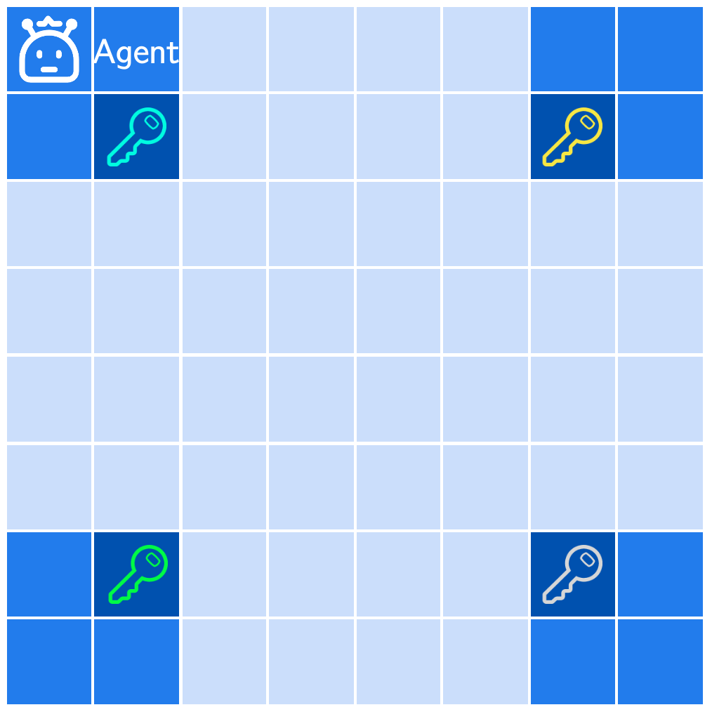
We first conduct a series of experiments in the GridWorld task introduced in Bengio et al. [2021a] to understand the effectiveness of Stochastic GFlowNets. An illustration of the task with size is shown in Figure 4. At each time step, the agent takes an action to navigate in the grid, where possible actions include operations to increase one coordinate and also a stop operation to terminate the episode, ensuring the underlying Markov decision process (MDP) is a directed acyclic graph. The agent obtains a reward as defined in Bengio et al. [2021a] when the trajectory ends at a terminal state . The reward function has modes located at the corners of the map as illustrated in Figure 4. The goal for the agent is to model the target reward distribution, and captures all the modes of the reward function. The shade of color in Figure 4 indicates the magnitude of rewards, where a darker color corresponds to a larger reward. We consider a variant with stochastic transition dynamics, where the randomness in the environment is injected following Machado et al. [2018], Yang et al. [2022] in GridWorld and all other benchmark tasks in Sections 4.2.1-4.2.3. Specifically, the environment transitions according to the selected action with probability , while with probability the environment executes a uniformly chosen action (like slipping to its neighboring regions randomly in Figure 4).
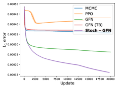
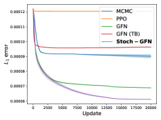
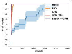
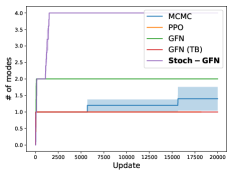
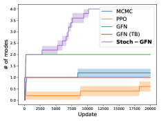
We compare Stochastic GFlowNet against vanilla GFlowNets trained with detailed balance (DB) [Bengio et al., 2021b] and trajectory balance (TB) [Malkin et al., 2022a] learning objectives, Metropolis-Hastings-MCMC [Xie et al., 2021], and PPO [Schulman et al., 2017] methods. We evaluate each method in terms of the empirical error defined as , with denoting the true reward distribution, and we estimate according to repeated sampling and calculating frequencies for visiting every possible state . We also compare them in terms of the number of modes discovered by each method during the course of training. Each algorithm is run for different seeds, and the performance is reported in its mean and standard deviation. We implement all baselines based on the open-source code111https://github.com/GFNOrg/gflownet, and a detailed description of the hyperparameters and setup can be found in Appendix A.1.
4.1.2 Performance Comparison
We now study the effectiveness of Stochastic GFNs on small, medium, and large GridWorlds with increasing sizes , and different levels of stochasticity.
Varying sizes of the map.
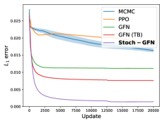
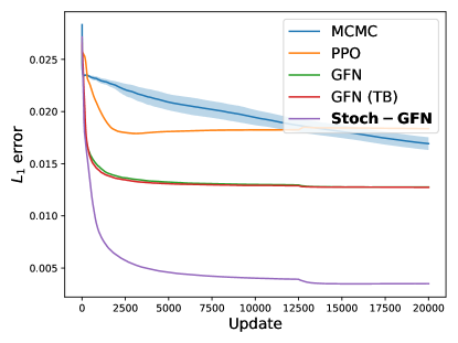
Figure 5 demonstrates the empirical error for each method in GridWorld (with a stochasticity level of ) with increasing sizes. As shown, MCMC does not perform well and PPO fails to converge. We also observe that the performance of TB gets much worse as the size of the problem increases, which may be attributed to a larger gradient variance [Madan et al., 2022]. Stochastic GFlowNets significantly outperform the baselines, and converge fastest and to the lowest empirical error. Figure 6 illustrates the number of modes discovered by each method during the course of training. As demonstrated, in stochastic environments (where the original convergence guarantees of GFlowNets do not hold), existing GFlowNet methods including DB and TB fail to discover all of the modes in maps with larger sizes. It is also worth noting that TB performs much worse than DB in terms of the number of modes discovered with increasing sizes of the maps, as it is optimized on the trajectory level with a sampled trajectory instead of the transition level as in DB, and can induce large variance. The proposed Stochastic GFlowNet method outperforms previous GFlowNet methods as well as MCMC and PPO by a large margin, while being able to efficiently discover different modes in maps with different sizes.
Varying stochasticity levels.
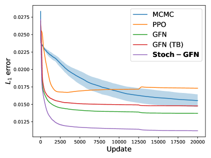
In Figure 7, we compare different methods in a small GridWorld with an increasing level of stochasticity . We observe that TB also fails to learn well with an increasing , and performs worse than DB besides the decreased performance with increasing sizes. On the other hand, Stochastic GFlowNets outperform the baselines by a significant margin, and are robust to higher levels of stochasticity, successfully handling stochastic transition dynamics.
4.1.3 Compatibility with Different GFlowNet Learning Objectives
In this section, we study Stochastic GFlowNets with the trajectory balance (TB) objective as described in Section 3.2. We evaluate Stochastic TB in GridWorlds with different sizes (including small with and large with ) and stochasticity levels (including low with and high with ). Specifically, Figure 8(a) corresponds to the result in a small map with a low stochasticity level, Figure 8(b) illustrates the results in a large map with a low stochasticity level, while Figure 8 shows the results in a small map with a high stochasticity level.
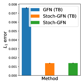
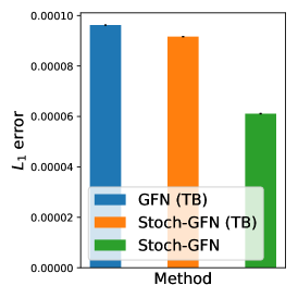
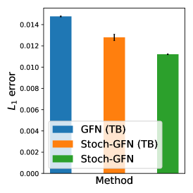
As shown in Figure 8, Stochastic TB (abbreviated as Stoch-GFN (TB) in the figure) greatly improves the performance of TB, validating the effectiveness of our proposed methodology. However, we observe that it underperforms relative to Stochastic DB when the scale of the problem increases or with a higher level of stochasticity (Figure 8(c)), which can be attributed to the larger variance of TB [Madan et al., 2022] in stochastic environments.
4.2 Autoregressive Sequence Generation
In this section, we study Stochastic GFN on autoregressive sequence generation tasks [Malkin et al., 2022a]. We first consider a bit sequence generation task to investigate the effect of the size of the action space and length of the trajectory with varying levels of environment stochasticity. We then study the more realistic and complex tasks of generating biological sequences.
4.2.1 Bit Sequences
Task.
In the bit sequence generation task [Malkin et al., 2022a], the agent aims to generate bit sequences of length . At each step, the agent appends a -bit “word" from a vocabulary to the current state from left to right, which is a partial sequence. Note that we consider a stochastic variant of the task, with noise level as described in Section 4.1.1. The resulting action space has a size of , and the length of the complete trajectories is . Following Malkin et al. [2022a], we define the reward function to have modes at a fixed set of bit sequences with , where is the edit distance. We evaluate each method in terms of the number of modes discovered during the course of training.
We study the performance of Stochastic DB with different levels of stochasticity, and compare it against vanilla DB and strong baselines including Advantage Actor-Critic (A2C) [Mnih et al., 2016], Soft Actor-Critic (SAC) [Haarnoja et al., 2018], and MCMC [Xie et al., 2021]. Each method is run for different seeds and we report the mean and standard deviation. More details about the experimental setup in the stochastic bit sequence generation task can be found in Appendix A.2. We use the same hyperparameters and architectures as in Malkin et al. [2022a].
Results.
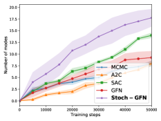
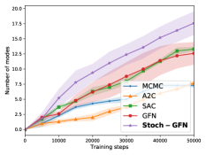
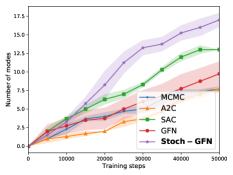
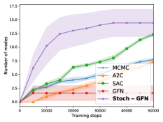
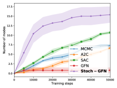
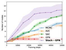
Figure 9 demonstrates the number of modes captured by each method throughout the training process with different levels of stochasticity ranging from to , where the first and second rows correspond to the results for and , respectively. We observe that regular GFlowNets (GFN in the figure) fail to learn well, particularly when the trajectories are longer (with a smaller value of ). On the other hand, the Stochastic GFlowNet (Stoch-GFN in the figures) is robust to increasing trajectory lengths, and also performs well when the stochasticity level increases. In addition, Stoch-GFN significantly outperforms strong baselines including MCMC, A2C, and SAC, discovering more modes faster.
4.2.2 TF Bind 8 Generation
Task.
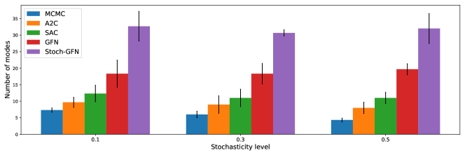
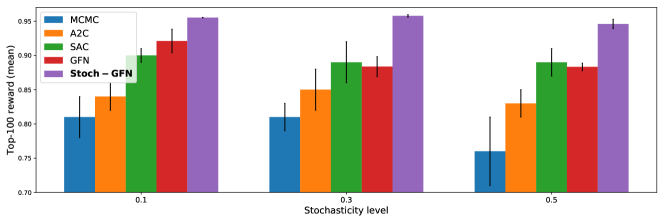
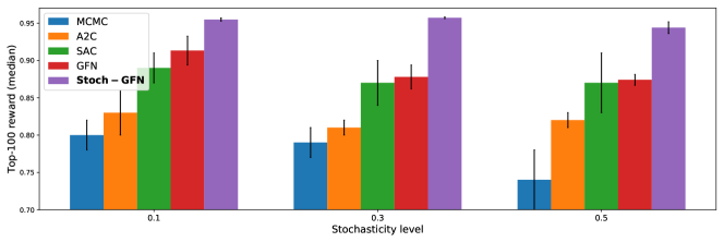
We now consider the practical task of generating DNA sequences with high binding activity with particular transcription factors, following Jain et al. [2022a]. At each time step, the agent appends a symbol from the vocabulary to the right of the current state. As with the bit generation task, we consider a stochastic variant of the task following Yang et al. [2022] with random actions taken with probability (as described in Section 4.1.1). We adopt a pre-trained neural network as the reward function following Jain et al. [2022a] that estimates the binding activity. We investigate how well Stochastic DB performs by comparing it with vanilla DB, MCMC, and RL-based methods including A2C and SAC. For evaluation, we evaluate each method in terms of the number of modes with rewards above a threshold discovered in the batch of generated sequences. We also use the mean reward and 50th percentile score for the top sequences ranked by their rewards from a batch of generated sequences for each method as in [Jain et al., 2022a, Trabucco et al., 2022]. We run each algorithm for different seeds, and report their mean and standard deviation. We follow the same hyperparameters, architectures, and setup as in Jain et al. [2022a], and a detailed description of the setup can be found in Appendix A.3.
Results.
Comparison results of Stoch-GFN and baselines with varying stochasticity levels (ranging from to ) in terms of the number of modes discovered with rewards above a threshold during the training process and top- mean rewards are summarized in Figure 10. As shown in Figure 10(a), Stoch-GFN discovers many more modes than GFN, MCMC, and RL-based methods in different stochasticity levels. Stoch-GFN also achieves higher top- rewards (in mean and median) than baselines as demonstrated in Figures 10(b)-(c), where the top- reward of GFN decrease with an increasing stochastic level. These results validate the effectiveness of Stoch-GFN in the more realistic task for biological sequence design with stochasticity in the environment.
4.2.3 Antimicrobial Peptide Generation
Task.
In this section, we study the realistic task of generating peptide sequences with anti-microbial properties [Malkin et al., 2022a, Jain et al., 2022a]. The agent chooses a symbol from the vocabulary that consists of amino acids and a special end-of-sequence action to the current state in a left-to-right manner at each time step. The maximum length of the sequence is , and the size of the resulting state space is . We consider a stochastic variant of the task (as in Section 4.1.1) with a stochasticity level of . The reward function is a pre-trained neural network that estimates the anti-microbial activity following [Malkin et al., 2022a] from the DBAASP database [Pirtskhalava et al., 2021]. As in Section 4.2.2, we generate sequences from each method and evaluate them in terms of the top- rewards and the number of modes discovered above a threshold. We study the performance of Stochastic DB by comparing it with DB, MCMC, and RL-based methods. We report the mean and standard deviation over runs for each method. A detailed description of the setup is in Appendix A.4 following Malkin et al. [2022a].
Results.
As shown in Table 1, we observe that Stoch-GFN significantly outperforms GFN and other baselines in terms of the top- reward. In addition, it also discovers more modes with rewards above a threshold than baseline methods, which further validates its effectiveness on the more complex and challenging task.
| Top- reward | Number of modes | |
| MCMC | ||
| A2C | ||
| SAC | ||
| GFN | ||
| Stoch-GFN |
5 Related Work
GFlowNets.
The universality and effectiveness of GFlowNets have been demonstrated in various kinds of applications, including biological sequence design [Jain et al., 2022a], causal discovery and structure learning [Deleu et al., 2022, Nishikawa-Toomey et al., 2022], substructure learning of deep neural network weights via Dropout [Liu et al., 2022], multi-objective optimization [Jain et al., 2022b], and robust job scheduling problems [Zhang et al., 2023a]. Malkin et al. [2022a] proposed the trajectory balance (TB) objective to optimize GFlowNet at a trajectory level instead of at the transition level as in detailed balance Bengio et al. [2021b], but can induce large variance, where the problem is exacerbated in stochastic environments. Madan et al. [2022] propose the sub-trajectory balance method considers sub-trajectories. The early GFlowNet proposals from Bengio et al. [2021a, b] first formulated GFlowNets and pointed out possible future development directions. Originating from reinforcement learning, GFlowNets face the same long-term credit assignment challenges to propagate downstream reward signals to earlier states. Pan et al. [2023] proposed a forward-looking GFlowNet formulation to exploit intermediate energies or rewards for more efficient credit assignment, making it possible to learn from incomplete trajectories. Pan et al. [2022] incorporates intrinsic intermediate rewards into GFlowNets by augmenting the flow values for better exploration. EB-GFN [Zhang et al., 2022b] jointly learns from data an energy/reward function along with the corresponding GFlowNet. Zhang et al. [2022a] recently points out that the relationship between generative models and GFlowNets. It is worth mentioning that Zhang et al. [2023b] shares a similar goal to our work; it extends the GFlowNet framework for stochastic reward settings with distributional modeling, while this work focuses on stochasticity in the environment transition dynamics.
Model-based Reinforcement Learning.
Model-based reinforcement learning (RL) is a promising approach for improved sample efficiency compared with model-free (RL) methods [Lillicrap et al., 2015, Fujimoto et al., 2018], and has been successfully applied to many tasks such as robotics leveraging different dynamics models. The stochastic value gradient method [Heess et al., 2015] learns a hybrid of model-based and model-free RL which can learn stochastic policies in stochastic continuous control tasks. Dreamer [Hafner et al., 2019] learns latent dynamics to solve long-horizon tasks from high-dimensional images. MuZero [Antonoglou et al., 2021] combines model-based methods with Monte-Carlo tree search for planning, and it has achieved great success in game playing. Stochastic MuZero [Schrittwieser et al., 2020] learns a stochastic model for extending MuZero to stochastic environments.
6 Conclusion
In this paper, we introduce a new methodology, Stochastic GFlowNets, which is the first empirically effective approach to extend GFlowNets to the more general and realistic stochastic environments, where existing GFlowNet methods can fail. Our method learns the GFlowNet policy and also the environment model to capture the stochasticity in the environment. We conduct extensive experiments in standard tasks for benchmarking GFlowNets with stochastic transition dynamics. Results show that Stochastic GFlowNet learns significantly better than previous methods in the presence of stochastic transitions. It is interesting for future work to study advanced model-based approaches for approximating the transition dynamics, and also apply our method to other challenging real-world tasks.
Acknowledgements
The authors would like to thank Almer Van der Sloot, Kanika Madan, and Qingpeng Cai for insightful discussions about the paper and the baselines in the AMP generation task. Longbo Huang is supported in part by the Technology and Innovation Major Project of the Ministry of Science and Technology of China under Grant 2020AAA0108400 and 2020AAA0108403, and Tsinghua Precision Medicine Foundation 10001020109. Yoshua Bengio acknowledges the funding from CIFAR, Genentech, Samsung, and IBM.
References
- Andrieu et al. [2003] Christophe Andrieu, Nando De Freitas, Arnaud Doucet, and Michael I Jordan. An introduction to mcmc for machine learning. Machine learning, 50(1):5–43, 2003.
- Antonoglou et al. [2021] Ioannis Antonoglou, Julian Schrittwieser, Sherjil Ozair, Thomas K Hubert, and David Silver. Planning in stochastic environments with a learned model. In International Conference on Learning Representations, 2021.
- Bengio et al. [2021a] Emmanuel Bengio, Moksh Jain, Maksym Korablyov, Doina Precup, and Yoshua Bengio. Flow network based generative models for non-iterative diverse candidate generation. Advances in Neural Information Processing Systems, 34:27381–27394, 2021a.
- Bengio et al. [2021b] Yoshua Bengio, Salem Lahlou, Tristan Deleu, Edward Hu, Mo Tiwari, and Emmanuel Bengio. GFlowNet foundations. arXiv preprint 2111.09266, 2021b.
- Deleu et al. [2022] Tristan Deleu, António Góis, Chris Emezue, Mansi Rankawat, Simon Lacoste-Julien, Stefan Bauer, and Yoshua Bengio. Bayesian structure learning with generative flow networks. Uncertainty in Artificial Intelligence (UAI), 2022.
- Fujimoto et al. [2018] Scott Fujimoto, Herke Hoof, and David Meger. Addressing function approximation error in actor-critic methods. In International conference on machine learning, pages 1587–1596. PMLR, 2018.
- Goodfellow et al. [2014] Ian Goodfellow, Jean Pouget-Abadie, Mehdi Mirza, Bing Xu, David Warde-Farley, Sherjil Ozair, Aaron Courville, and Yoshua Bengio. Generative adversarial nets. Neural Information Processing Systems (NIPS), pages 2672–2680, 2014.
- Haarnoja et al. [2017] Tuomas Haarnoja, Haoran Tang, Pieter Abbeel, and Sergey Levine. Reinforcement learning with deep energy-based policies. International Conference on Machine Learning (ICML), 2017.
- Haarnoja et al. [2018] Tuomas Haarnoja, Aurick Zhou, Pieter Abbeel, and Sergey Levine. Soft actor-critic: Off-policy maximum entropy deep reinforcement learning with a stochastic actor. International Conference on Machine Learning (ICML), 2018.
- Hafner et al. [2019] Danijar Hafner, Timothy Lillicrap, Jimmy Ba, and Mohammad Norouzi. Dream to control: Learning behaviors by latent imagination. arXiv preprint arXiv:1912.01603, 2019.
- Hastings [1970] W Keith Hastings. Monte carlo sampling methods using markov chains and their applications. 1970.
- Heess et al. [2015] Nicolas Heess, Gregory Wayne, David Silver, Timothy Lillicrap, Tom Erez, and Yuval Tassa. Learning continuous control policies by stochastic value gradients. Advances in neural information processing systems, 28, 2015.
- Ho et al. [2020] Jonathan Ho, Ajay Jain, and Pieter Abbeel. Denoising diffusion probabilistic models. Advances in Neural Information Processing Systems, 33:6840–6851, 2020.
- Jain et al. [2022a] Moksh Jain, Emmanuel Bengio, Alex Hernandez-Garcia, Jarrid Rector-Brooks, Bonaventure F.P. Dossou, Chanakya Ekbote, Jie Fu, Tianyu Zhang, Micheal Kilgour, Dinghuai Zhang, Lena Simine, Payel Das, and Yoshua Bengio. Biological sequence design with GFlowNets. International Conference on Machine Learning (ICML), 2022a.
- Jain et al. [2022b] Moksh Jain, Sharath Chandra Raparthy, Alex Hernandez-Garcia, Jarrid Rector-Brooks, Yoshua Bengio, Santiago Miret, and Emmanuel Bengio. Multi-objective gflownets. arXiv preprint arXiv:2210.12765, 2022b.
- Kingma and Ba [2015] Diederik P Kingma and Jimmy Ba. Adam: A method for stochastic optimization. International Conference on Learning Representations (ICLR), 2015.
- Kingma and Welling [2013] Diederik P Kingma and Max Welling. Auto-encoding variational bayes. arXiv preprint arXiv:1312.6114, 2013.
- Kunaver and Požrl [2017] Matevž Kunaver and Tomaž Požrl. Diversity in recommender systems–a survey. Knowledge-based systems, 123:154–162, 2017.
- Lillicrap et al. [2015] Timothy P Lillicrap, Jonathan J Hunt, Alexander Pritzel, Nicolas Heess, Tom Erez, Yuval Tassa, David Silver, and Daan Wierstra. Continuous control with deep reinforcement learning. arXiv preprint arXiv:1509.02971, 2015.
- Liu et al. [2022] Dianbo Liu, Moksh Jain, Bonaventure F. P. Dossou, Qianli Shen, Salem Lahlou, Anirudh Goyal, Nikolay Malkin, Chris C. Emezue, Dinghuai Zhang, Nadhir Hassen, Xu Ji, Kenji Kawaguchi, and Yoshua Bengio. Gflowout: Dropout with generative flow networks. ArXiv, abs/2210.12928, 2022.
- Machado et al. [2018] Marlos C Machado, Marc G Bellemare, Erik Talvitie, Joel Veness, Matthew Hausknecht, and Michael Bowling. Revisiting the arcade learning environment: Evaluation protocols and open problems for general agents. Journal of Artificial Intelligence Research, 61:523–562, 2018.
- Madan et al. [2022] Kanika Madan, Jarrid Rector-Brooks, Maksym Korablyov, Emmanuel Bengio, Moksh Jain, Andrei Nica, Tom Bosc, Yoshua Bengio, and Nikolay Malkin. Learning GFlowNets from partial episodes for improved convergence and stability. ICLR’2023; arXiv:2209.12782, 2022.
- Malkin et al. [2022a] Nikolay Malkin, Moksh Jain, Emmanuel Bengio, Chen Sun, and Yoshua Bengio. Trajectory balance: Improved credit assignment in GFlowNets. Neural Information Processing Systems (NeurIPS), 2022a.
- Malkin et al. [2022b] Nikolay Malkin, Salem Lahlou, Tristan Deleu, Xu Ji, Edward Hu, Katie Everett, Dinghuai Zhang, and Yoshua Bengio. Gflownets and variational inference. arXiv preprint arXiv:2210.00580, 2022b.
- Metropolis et al. [1953] Nicholas Metropolis, Arianna W Rosenbluth, Marshall N Rosenbluth, Augusta H Teller, and Edward Teller. Equation of state calculations by fast computing machines. The journal of chemical physics, 21(6):1087–1092, 1953.
- Mnih et al. [2015] Volodymyr Mnih, Koray Kavukcuoglu, David Silver, Andrei A Rusu, Joel Veness, Marc G Bellemare, Alex Graves, Martin Riedmiller, Andreas K Fidjeland, Georg Ostrovski, et al. Human-level control through deep reinforcement learning. nature, 518(7540):529–533, 2015.
- Mnih et al. [2016] Volodymyr Mnih, Adria Puigdomenech Badia, Mehdi Mirza, Alex Graves, Timothy Lillicrap, Tim Harley, David Silver, and Koray Kavukcuoglu. Asynchronous methods for deep reinforcement learning. Neural Information Processing Systems (NIPS), 2016.
- Nishikawa-Toomey et al. [2022] Mizu Nishikawa-Toomey, Tristan Deleu, Jithendaraa Subramanian, Yoshua Bengio, and Laurent Charlin. Bayesian learning of causal structure and mechanisms with GFlowNets and variational bayes. arXiv preprint 2211.02763, 2022.
- Pan et al. [2022] Ling Pan, Dinghuai Zhang, Aaron Courville, Longbo Huang, and Yoshua Bengio. Generative augmented flow networks. arXiv preprint 2210.03308, 2022.
- Pan et al. [2023] Ling Pan, Nikolay Malkin, Dinghuai Zhang, and Yoshua Bengio. Better training of gflownets with local credit and incomplete trajectories. ArXiv, abs/2302.01687, 2023.
- Paster et al. [2022] Keiran Paster, Sheila McIlraith, and Jimmy Ba. You can’t count on luck: Why decision transformers fail in stochastic environments. arXiv preprint arXiv:2205.15967, 2022.
- Pirtskhalava et al. [2021] Malak Pirtskhalava, Anthony A Amstrong, Maia Grigolava, Mindia Chubinidze, Evgenia Alimbarashvili, Boris Vishnepolsky, Andrei Gabrielian, Alex Rosenthal, Darrell E Hurt, and Michael Tartakovsky. Dbaasp v3: database of antimicrobial/cytotoxic activity and structure of peptides as a resource for development of new therapeutics. Nucleic acids research, 49(D1):D288–D297, 2021.
- Schrittwieser et al. [2020] Julian Schrittwieser, Ioannis Antonoglou, Thomas Hubert, Karen Simonyan, Laurent Sifre, Simon Schmitt, Arthur Guez, Edward Lockhart, Demis Hassabis, Thore Graepel, et al. Mastering atari, go, chess and shogi by planning with a learned model. Nature, 588(7839):604–609, 2020.
- Schulman et al. [2017] John Schulman, Filip Wolski, Prafulla Dhariwal, Alec Radford, and Oleg Klimov. Proximal policy optimization algorithms. arXiv preprint 1707.06347, 2017.
- Song et al. [2021] Li-Fu Song, Zheng-Hua Deng, Zi-Yi Gong, Lu-Lu Li, and Bing-Zhi Li. Large-scale de novo oligonucleotide synthesis for whole-genome synthesis and data storage: Challenges and opportunities. Frontiers in bioengineering and biotechnology, 9:689797, 2021.
- Sutton and Barto [2018] Richard S Sutton and Andrew G Barto. Reinforcement learning: An introduction. MIT press, 2018.
- Trabucco et al. [2022] Brandon Trabucco, Xinyang Geng, Aviral Kumar, and Sergey Levine. Design-bench: Benchmarks for data-driven offline model-based optimization. In International Conference on Machine Learning, pages 21658–21676. PMLR, 2022.
- Vaswani et al. [2017] Ashish Vaswani, Noam Shazeer, Niki Parmar, Jakob Uszkoreit, Llion Jones, Aidan N Gomez, Łukasz Kaiser, and Illia Polosukhin. Attention is all you need. Neural Information Processing Systems (NIPS), 2017.
- Venkatraman et al. [2015] Arun Venkatraman, Martial Hebert, and J Bagnell. Improving multi-step prediction of learned time series models. In Proceedings of the AAAI Conference on Artificial Intelligence, volume 29, 2015.
- Xie et al. [2021] Yutong Xie, Chence Shi, Hao Zhou, Yuwei Yang, Weinan Zhang, Yong Yu, and Lei Li. Mars: Markov molecular sampling for multi-objective drug discovery. arXiv preprint arXiv:2103.10432, 2021.
- Yang et al. [2022] Mengjiao Yang, Dale Schuurmans, Pieter Abbeel, and Ofir Nachum. Dichotomy of control: Separating what you can control from what you cannot. arXiv preprint arXiv:2210.13435, 2022.
- Zhang et al. [2023a] David Zhang, Corrado Rainone, Markus Peschl, and Roberto Bondesan. Robust scheduling with GFlowNets. International Conference on Learning Representations (ICLR), 2023a.
- Zhang et al. [2022a] Dinghuai Zhang, Ricky T. Q. Chen, Nikolay Malkin, and Yoshua Bengio. Unifying generative models with GFlowNets. arXiv preprint 2209.02606, 2022a.
- Zhang et al. [2022b] Dinghuai Zhang, Nikolay Malkin, Zhen Liu, Alexandra Volokhova, Aaron Courville, and Yoshua Bengio. Generative flow networks for discrete probabilistic modeling. International Conference on Machine Learning (ICML), 2022b.
- Zhang et al. [2023b] Dinghuai Zhang, Ling Pan, Ricky TQ Chen, Aaron Courville, and Yoshua Bengio. Distributional gflownets with quantile flows. arXiv preprint arXiv:2302.05793, 2023b.
Appendix A Experimental Details
A.1 Gridworld
The reward function for GridWorld is defined as in Eq. (11) following Bengio et al. [2021a], where , , and .
| (11) |
We use a feedforward network that consists of two hidden layers with hidden units and LeakyReLU activation. States are represented using one-hot embeddings. As for the environment model in Stochastic GFlowNet, it is also a feedforward layer consisting of two hidden layers with hidden units and LeakyReLU activation. All models are trained for iterations, and we use a parallel of rollouts in the environment at each iteration (which are then stored in the experience replay buffer). The GFlowNet model is updated based on the rollouts, and we train it based on the Adam [Kingma and Ba, 2015] optimizer using a learning rate of (the learning rate for in TB is ). We train the environment model using data sampled from the experience replay buffer with a batch size of , which is trained using the Adam optimizer with a learning rate of . MCMC and PPO use the same configuration as in Bengio et al. [2021a].
A.2 Bit Sequences
We follow the same setup for the bit sequence generation task as in Malkin et al. [2022a]. The GFlowNet model is a Transformer [Vaswani et al., 2017] that consists of hidden layers with hidden units and uses attention heads. The exploration strategy is -greedy with , while the sampling temperature is set to . It uses a reward exponent of . The learning rate for training the GFlowNet model is , with a batch size of . As for the environment model in Stochastic GFlowNet, we use a feedforward network consisting of two hidden layers with hidden units and ReLU activation, which is trained using the Adam optimizer with a learning rate of . It is trained using data sampled from the experience replay buffer with a batch size of . We train all models for iterations, using a parallel of rollouts in the environment. MCMC, A2C, and SAC adopt the same configuration as in Malkin et al. [2022a].
A.3 TFBind-8
For the TFBind-8 generation task, we follow the same setup as in Jain et al. [2022a]. The vocabulary consists of nucleobases, and the trajectory length is . The GFlowNet model is a feedforward network that consists of hidden layers with hidden units and ReLU activation. The exploration strategy is -greedy with , while the reward exponent is . The learning rate for training the GFlowNet model is , with a batch size of . As for the environment model, we use a feedforward network consisting of two hidden layers with hidden units and ReLU activation, which is trained using the Adam optimizer with a learning rate of . It is trained using data sampled from the experience replay buffer with a batch size of . We train all models for iterations. MCMC, A2C, and SAC baselines follow the same configuration as in Jain et al. [2022a].
A.4 Antimicrobial Peptide Generation
We follow the same setup for the antimicrobial peptide generation task as in Malkin et al. [2022a]. The GFlowNet model is a Transformer [Vaswani et al., 2017] that consists of hidden layers with hidden units and uses attention heads. The exploration strategy is -greedy with , while the sampling temperature is set to . It uses a reward exponent of . The learning rate for training the GFlowNet model is , with a batch size of . As for the environment model, we use a feedforward network consisting of two hidden layers with hidden units and ReLU activation, which is trained using the Adam optimizer with a learning rate of . It is trained using data sampled from the experience replay buffer with a batch size of . We train all models for iterations, using a parallel of rollouts in the environment.