Convergence rate for the

longest T𝑇T-contaminated runs of heads.

Paper with detailed proofs

IstvΓ‘n Fazekas,111fazekas.istvan@inf.unideb.huΒ BorbΓ‘la Fazekas, Β Michael Ochieng Suja

University of Debrecen, Hungary

Abstract

We study the length of T𝑇T-contaminated runs of heads in the well-known coin tossing experiment. A T𝑇T-contaminated run of heads is a sequence of consecutive heads interrupted by T𝑇T tails. For T=1𝑇1T=1 and T=2𝑇2T=2 we find the asymptotic distribution for the first hitting time of the T𝑇T contaminated run of heads having length mπ‘šm; furthermore, we obtain a limit theorem for the length of the longest T𝑇T-contaminated head run. We prove that the rate of the approximation of our accompanying distribution for the length of the longest T𝑇T-contaminated head run is considerably better than the previous ones. For the proof we use a powerful lemma by CsΓ‘ki, FΓΆldes and KomlΓ³s, see [1].

1 Introduction

In this paper, we shall consider the well-known coin tossing experiment. Let p𝑝p denote the probability of heads, so the probability of tails is q=1βˆ’pπ‘ž1𝑝q=1-p. We toss the coin N𝑁N times.

We shall study the length of consecutive heads interrupted by T𝑇T tails. A subsequence containing T𝑇T tails while all the other values are heads will be called a T𝑇T-contaminated run of heads.

The most famous known results concern the length of the pure head runs. The case of the fair coin was studied in the classical paper of ErdΕ‘s and RΓ©nyi [2]. Later several papers were published on this topic. E.g. [9] studied the accuracy of the approximation to the distribution of the length of the longest head run in a Markov chain (see also the references in [9]).

An early paper obtaining almost sure limit results for the length of the longest runs containing at most T𝑇T tails is [3]. Later several papers were devoted to the topic. FΓΆldes, in [5], presented asymptotic results for the distribution of the number of T𝑇T-contaminated head runs, the first hitting time of a T𝑇T-contaminated head run having a fixed length, and the length of the longest T𝑇T-contaminated head run. MΓ³ri in [8] obtained a so called almost sure limit theorem for the longest T𝑇T-contaminated head run.

In the paper [6], Gordon, Schilling, and Waterman applied extreme value theory to obtain the asymptotic behaviour of the expectation and the variance of the length of the longest T𝑇T-contaminated head run. Also in [6], accompanying distributions were obtained for the length of the longest T𝑇T-contaminated head run. In [4], it was shown that the accompanying distributions of [6] can be obtained by the method of FΓΆldes [5].

After minor algebraic manipulation, Theorem 1 of [6] states the following.

Proposition 1.1.

Let μ​(N)πœ‡π‘\mu(N) denote the length of the longest T𝑇T-contaminated run of heads during the coin tossing experiment of length N𝑁N. Let

m0​(N)=log⁑(q​N)+T​log⁑(log⁑(q​N))+T​log⁑(q/p)βˆ’log⁑(T!),subscriptπ‘š0π‘π‘žπ‘π‘‡π‘žπ‘π‘‡π‘žπ‘π‘‡m_{0}(N)=\log(qN)+T\log(\log(qN))+T\log(q/p)-\log(T!), (1.1)

where log\log denotes the logarithm of base 1/p1𝑝1/p. Let [m0​(N)]delimited-[]subscriptπ‘š0𝑁[m_{0}(N)] denote the integer part of m0​(N)subscriptπ‘š0𝑁m_{0}(N) and let {m0​(N)}subscriptπ‘š0𝑁\{m_{0}(N)\} denote the fractional part of m0​(N)subscriptπ‘š0𝑁m_{0}(N). Then

P​(μ​(N)βˆ’[m0​(N)]<k)=exp⁑(βˆ’pkβˆ’{m0​(N)})+o​(1).π‘ƒπœ‡π‘delimited-[]subscriptπ‘š0π‘π‘˜superscriptπ‘π‘˜subscriptπ‘š0𝑁o1P\left(\mu(N)-[m_{0}(N)]<k\right)=\exp\left(-p^{k-\{m_{0}(N)\}}\right)+\rm{o}(1).

However, numerical experiments show that the approximation offered by Proposition 1.1 is quite weak. Therefore the aim of this paper is to improve the above result for the most important cases of T=1𝑇1T=1 and T=2𝑇2T=2.

Our main result is Theorem 2.2. Like Proposition 1.1, our theorem offers an accompanying distribution sequence for the distribution of the centralized version of μ​(N)πœ‡π‘\mu(N). We show that the rate of the approximation in our new theorem is O​(1/(log⁑(N))2)O1superscript𝑁2{\rm{O}}\left(1/(\log(N))^{2}\right). We shall see, that for T=1𝑇1T=1 and T=2𝑇2T=2 the rate of the approximation in Proposition 1.1 is O​(log⁑(log⁑(N))/log⁑(N))O𝑁𝑁{\rm{O}}\left(\log(\log(N))/\log(N)\right), so our result considerably improves the former result. We also obtain a result for the first hitting time of the T𝑇T contaminated run of heads having length mπ‘šm, see Theorem 2.1. In section 5 we present some simulation results supporting that our new approximation excels the former ones.

The main tool of the proof is a powerful lemma by CsΓ‘ki, FΓΆldes and KomlΓ³s, see [1]. We quote this lemma as Lemma 3.1. In order to apply this lemma, we need several elementary but quite long calculations, see lemmas 3.2, 3.3.

2 The first hitting time and the longest run

Consider the well-known coin tossing experiment. Let p𝑝p be the probability of heads and let q=1βˆ’pπ‘ž1𝑝q=1-p be the probability of tails. Here p𝑝p is a fixed number with 0<p<10𝑝10<p<1. We toss a coin N𝑁N times independently. As usual, we shall write 111 for heads and 00 for tails. So we shall consider independent identically distributed random variables X1,X2,…,XNsubscript𝑋1subscript𝑋2…subscript𝑋𝑁X_{1},X_{2},\dots,X_{N} with P​(Xi=1)=p𝑃subscript𝑋𝑖1𝑝P(X_{i}=1)=p and P​(Xi=0)=q𝑃subscript𝑋𝑖0π‘žP(X_{i}=0)=q, i=1,2,…,N𝑖12…𝑁i=1,2,\dots,N.

Let Tβ‰₯0𝑇0T\geq 0 be a fixed non-negative integer. We shall study the T𝑇T-interrupted runs of heads. It means that there are T𝑇T zeros in an mπ‘šm length sequence of ones and zeros. So let mπ‘šm be a positive integer. Let denote An=An,msubscript𝐴𝑛subscriptπ΄π‘›π‘šA_{n}=A_{n,m} the event that there are precisely T𝑇T zeros in the sequence Xn,Xn+1,…,Xn+mβˆ’1subscript𝑋𝑛subscript𝑋𝑛1…subscriptπ‘‹π‘›π‘š1X_{n},X_{n+1},\dots,X_{n+m-1}. So An,msubscriptπ΄π‘›π‘šA_{n,m} is the event that there is a T𝑇T-interrupted run of ones at positions n,n+1,…,n+mβˆ’1𝑛𝑛1β€¦π‘›π‘š1n,{n+1},\dots,{n+m-1}.

Let Ο„msubscriptπœπ‘š\tau_{m} be the first hitting time of the T𝑇T-contaminated run of heads having length mπ‘šm. We shall find the asymptotic distribution of Ο„msubscriptπœπ‘š\tau_{m} as mβ†’βˆžβ†’π‘šm\to\infty for T=1𝑇1T=1 and for T=2𝑇2T=2.

Theorem 2.1.

Let T=1𝑇1T=1 or T=2𝑇2T=2, 0<p<10𝑝10<p<1. Let Ο„msubscriptπœπ‘š\tau_{m} be the first hitting time of the T𝑇T contaminated run of heads having length mπ‘šm. Then, for x>0π‘₯0x>0,

P​(Ο„m​α​P​(A1)>x)∼eβˆ’xsimilar-to𝑃subscriptπœπ‘šπ›Όπ‘ƒsubscript𝐴1π‘₯superscript𝑒π‘₯P(\tau_{m}\alpha P(A_{1})>x)\sim e^{-x}

as mβ†’βˆžβ†’π‘šm\to\infty. Here if T=1𝑇1T=1, then Ξ±=q+2​pmβˆ’1βˆ’1mπ›Όπ‘ž2superscriptπ‘π‘š11π‘š\alpha=q+\frac{2p^{m-1}-1}{m} and P​(A1)=m​pmβˆ’1​q𝑃subscript𝐴1π‘šsuperscriptπ‘π‘š1π‘žP(A_{1})=mp^{m-1}q. When T=2𝑇2T=2, then Ξ±=qβˆ’2mπ›Όπ‘ž2π‘š\alpha=q-\frac{2}{m}, P​(A1)=(m2)​pmβˆ’2​q2𝑃subscript𝐴1binomialπ‘š2superscriptπ‘π‘š2superscriptπ‘ž2P(A_{1})={m\choose 2}p^{m-2}q^{2}.

Remark 2.1.

One can show, that Theorem 2.1 is valid for T=2𝑇2T=2 with Ξ±=qβˆ’2m+2​(mβˆ’2)m​pmβˆ’2βˆ’2​(mβˆ’4)m​pmβˆ’1π›Όπ‘ž2π‘š2π‘š2π‘šsuperscriptπ‘π‘š22π‘š4π‘šsuperscriptπ‘π‘š1\alpha=q-\frac{2}{m}+\frac{2(m-2)}{m}p^{m-2}-\frac{2(m-4)}{m}p^{m-1}, too (see Remark 3.4).

Now, we turn to the length of the longest contaminated run of heads.

Theorem 2.2.

Let T=1𝑇1T=1 or T=2𝑇2T=2, and let 0<p<10𝑝10<p<1 be fixed. Let μ​(N)πœ‡π‘\mu(N) be the length of the longest T𝑇T contaminated run of heads during tossing N𝑁N times a coin. Let

m​(N)π‘šπ‘\displaystyle m(N) =\displaystyle= log⁑(q​N)+T​log⁑(log⁑(q​N))+π‘žπ‘limit-fromπ‘‡π‘žπ‘\displaystyle\log(qN)+T\log(\log(qN))+
+\displaystyle+ T2​log⁑(log⁑(q​N))c​log⁑(q​N)βˆ’Tc​q0​log⁑(q​N)βˆ’T32​c​(log⁑(log⁑(q​N))log⁑(q​N))2+superscript𝑇2π‘žπ‘π‘π‘žπ‘π‘‡π‘subscriptπ‘ž0π‘žπ‘limit-fromsuperscript𝑇32𝑐superscriptπ‘žπ‘π‘žπ‘2\displaystyle T^{2}\frac{\log(\log(qN))}{c\log(qN)}-\frac{T}{cq_{0}\log(qN)}-\frac{T^{3}}{2c}\left(\frac{\log(\log(qN))}{\log(qN)}\right)^{2}+
+\displaystyle+ T2​log⁑(log⁑(q​N))c​q0​(log⁑(q​N))2+T3​log⁑(log⁑(q​N))(c​log⁑(q​N))2+superscript𝑇2π‘žπ‘π‘subscriptπ‘ž0superscriptπ‘žπ‘2limit-fromsuperscript𝑇3π‘žπ‘superscriptπ‘π‘žπ‘2\displaystyle T^{2}\frac{\log(\log(qN))}{cq_{0}(\log(qN))^{2}}+T^{3}\frac{\log(\log(qN))}{(c\log(qN))^{2}}+
+\displaystyle+ (T​log⁑(qp)βˆ’log⁑(T!))​(1+Tc​log⁑(q​N)βˆ’T2​log⁑(log⁑(q​N))c​(log⁑(q​N))2),π‘‡π‘žπ‘π‘‡1π‘‡π‘π‘žπ‘superscript𝑇2π‘žπ‘π‘superscriptπ‘žπ‘2\displaystyle\left(T\log\left(\frac{q}{p}\right)-\log(T!)\right)\left(1+\frac{T}{c\log(qN)}-T^{2}\frac{\log(\log(qN))}{c(\log(qN))^{2}}\right),

where log\log denotes the logarithm of base 1/p1𝑝1/p, c=ln⁑(1/p)𝑐1𝑝c=\ln(1/p), ln\ln denotes the natural logarithm of base e𝑒e, and q0=2​q2+T​qβˆ’qsubscriptπ‘ž02π‘ž2π‘‡π‘žπ‘žq_{0}=\frac{2q}{2+Tq-q}. Let [m​(N)]delimited-[]π‘šπ‘[m(N)] denote the integer part of m​(N)π‘šπ‘m(N), while {m​(N)}π‘šπ‘\{m(N)\} denotes the fractional part of m​(N)π‘šπ‘m(N), i.e. {m​(N)}=m​(N)βˆ’[m​(N)]π‘šπ‘π‘šπ‘delimited-[]π‘šπ‘\{m(N)\}=m(N)-[m(N)].

Then

P​(μ​(N)βˆ’[m​(N)]<k)=π‘ƒπœ‡π‘delimited-[]π‘šπ‘π‘˜absent\displaystyle P(\mu(N)-[m(N)]<k)= (2.2)
=eβˆ’p(kβˆ’{m​(N)})​(1βˆ’Tc​log⁑(q​N)+T2​log⁑(log⁑(q​N))c​(log⁑(q​N))2)​(1+O​(1(log⁑N)2))absentsuperscript𝑒superscriptπ‘π‘˜π‘šπ‘1π‘‡π‘π‘žπ‘superscript𝑇2π‘žπ‘π‘superscriptπ‘žπ‘21O1superscript𝑁2\displaystyle\qquad\qquad=e^{\displaystyle{-p^{(k-\{m(N)\})\left(1-\frac{T}{c\log(qN)}+T^{2}\frac{\log(\log(qN))}{c(\log(qN))^{2}}\right)}}}\left(1+{\rm{O}}\left(\frac{1}{(\log N)^{2}}\right)\right)

for any integer kπ‘˜k, where f​(N)=O​(h​(N))𝑓𝑁Oβ„Žπ‘f(N)={\rm{O}}(h(N)) means that f​(N)/h​(N)π‘“π‘β„Žπ‘f(N)/h(N) is bounded as Nβ†’βˆžβ†’π‘N\to\infty.

Remark 2.2.

Using our method, for T=1𝑇1T=1 and T=2𝑇2T=2 and for m0​(N)subscriptπ‘š0𝑁m_{0}(N) from (1.1), we obtain that the rate of convergence in Proposition 1.1 is O​(log⁑(log⁑(N))/log⁑(N))O𝑁𝑁{\rm{O}}\left(\log(\log(N))/\log(N)\right), that is

P​(μ​(N)βˆ’[m0​(N)]<k)=exp⁑(βˆ’pkβˆ’{m0​(N)})​(1+O​(log⁑(log⁑(N))/log⁑(N))).π‘ƒπœ‡π‘delimited-[]subscriptπ‘š0π‘π‘˜superscriptπ‘π‘˜subscriptπ‘š0𝑁1O𝑁𝑁P\left(\mu(N)-[m_{0}(N)]<k\right)=\exp\left(-p^{k-\{m_{0}(N)\}}\right)\left(1+{\rm{O}}\left(\log(\log(N))/\log(N)\right)\right).

So our Theorem considerably improves Theorem 1 of [6] in the cases of T=1𝑇1T=1 and T=2𝑇2T=2.

3 Preliminary Lemmas

The following lemma of [1] will play a fundamental role in our proofs.

Lemma 3.1.

(Main lemma, stationary case, finite form of CsΓ‘ki, FΓΆldes, KomlΓ³s [1].) Let X1,X2,…subscript𝑋1subscript𝑋2italic-…X_{1},X_{2},\dots be any sequence of independent random variables, and let β„±n,msubscriptβ„±π‘›π‘š\mathcal{F}_{n,m} be the ΟƒπœŽ\sigma-algebra generated by the random variables Xn,Xn+1,…,Xn+mβˆ’1subscript𝑋𝑛subscript𝑋𝑛1…subscriptπ‘‹π‘›π‘š1X_{n},X_{n+1},\dots,X_{n+m-1}. Let mπ‘šm be fixed and let An=An,mβˆˆβ„±n,msubscript𝐴𝑛subscriptπ΄π‘›π‘šsubscriptβ„±π‘›π‘šA_{n}=A_{n,m}\in\mathcal{F}_{n,m}. Assume that the sequence of events An=An,msubscript𝐴𝑛subscriptπ΄π‘›π‘šA_{n}=A_{n,m} is stationary, that is P​(Ai1+d​Ai2+d​⋯​Aik+d)𝑃subscript𝐴subscript𝑖1𝑑subscript𝐴subscript𝑖2𝑑⋯subscript𝐴subscriptπ‘–π‘˜π‘‘P(A_{i_{1}+d}A_{i_{2}+d}\cdots A_{i_{k}+d}) is independent of d𝑑d.

Assume that there is a fixed number α𝛼\alpha, 0<α≀10𝛼10<\alpha\leq 1, such that the following three conditions hold for some fixed kπ‘˜k with 2≀k≀m2π‘˜π‘š2\leq k\leq m, and fixed Ξ΅πœ€\varepsilon with 0<Ξ΅<min⁑{p/10,1/42}0πœ€π‘101420<\varepsilon<\min\{p/10,1/42\}

  1. (SI)
    |P(A2Β―β‹―AkΒ―|A1)βˆ’Ξ±|<Ξ΅,|P(\bar{A_{2}}\cdots\bar{A_{k}}|A_{1})-\alpha|<\varepsilon,
  2. (SII)
    βˆ‘k+1≀i≀2​mP​(Ai|A1)<Ξ΅,subscriptπ‘˜1𝑖2π‘šπ‘ƒconditionalsubscript𝐴𝑖subscript𝐴1πœ€\sum_{k+1\leq i\leq 2m}P(A_{i}|A_{1})<\varepsilon,
  3. (SIII)
    P​(A1)<Ξ΅/m.𝑃subscript𝐴1πœ€π‘šP(A_{1})<\varepsilon/m.

Then, for all N>1𝑁1N>1,

|P​(A2¯​⋯​AΒ―N|A1)P​(A2¯​⋯​AΒ―N)βˆ’Ξ±|<7​Ρ𝑃conditionalΒ―subscript𝐴2β‹―subscript¯𝐴𝑁subscript𝐴1𝑃¯subscript𝐴2β‹―subscript¯𝐴𝑁𝛼7πœ€\left|\frac{P(\bar{A_{2}}\cdots\bar{A}_{N}|A_{1})}{P(\bar{A_{2}}\cdots\bar{A}_{N})}-\alpha\right|<7\varepsilon

and

eβˆ’(Ξ±+10​Ρ)​N​P​(A1)βˆ’2​m​P​(A1)<P​(A1¯​⋯​AΒ―N)<eβˆ’(Ξ±βˆ’10​Ρ)​N​P​(A1)+2​m​P​(A1).superscript𝑒𝛼10πœ€π‘π‘ƒsubscript𝐴12π‘šπ‘ƒsubscript𝐴1𝑃¯subscript𝐴1β‹―subscript¯𝐴𝑁superscript𝑒𝛼10πœ€π‘π‘ƒsubscript𝐴12π‘šπ‘ƒsubscript𝐴1e^{-(\alpha+10\varepsilon)NP(A_{1})-2mP(A_{1})}<P(\bar{A_{1}}\cdots\bar{A}_{N})<e^{-(\alpha-10\varepsilon)NP(A_{1})+2mP(A_{1})}. (3.1)

First we present some preliminary results which can have their own interest. We shall check conditions (SI)-(SIII) of Lemma 3.1 if k=mπ‘˜π‘šk=m. Next remarks show that conditions (SII) and (SIII) are true for any T𝑇T if mπ‘šm is large enough.

Remark 3.1.

Consider condition (SIII). We show that (SIII) is true for any T𝑇T if mπ‘šm is large enough. We have

P​(A1)=(mT)​pmβˆ’T​qT≀mTT!​pmβˆ’T​qT<Ξ΅m,𝑃subscript𝐴1binomialπ‘šπ‘‡superscriptπ‘π‘šπ‘‡superscriptπ‘žπ‘‡superscriptπ‘šπ‘‡π‘‡superscriptπ‘π‘šπ‘‡superscriptπ‘žπ‘‡πœ€π‘šP(A_{1})={m\choose T}p^{m-T}q^{T}\leq\frac{m^{T}}{T!}p^{m-T}q^{T}<\frac{\varepsilon}{m},

if

mT+1​pm<Ρ​(pq)T​T!,superscriptπ‘šπ‘‡1superscriptπ‘π‘šπœ€superscriptπ‘π‘žπ‘‡π‘‡m^{T+1}p^{m}<\varepsilon\left(\frac{p}{q}\right)^{T}T!, (3.2)

and the last inequality is satisfied for any fixed positive Ξ΅πœ€\varepsilon if mπ‘šm is large enough. So we always can assume (SIII) of Lemma 3.1 for any T𝑇T.

Remark 3.2.

Consider condition (SII).

P​(Ai|A1)=P​(Ai)=(mT)​pmβˆ’T​qT≀mTT!​pmβˆ’T​qT,𝑃conditionalsubscript𝐴𝑖subscript𝐴1𝑃subscript𝐴𝑖binomialπ‘šπ‘‡superscriptπ‘π‘šπ‘‡superscriptπ‘žπ‘‡superscriptπ‘šπ‘‡π‘‡superscriptπ‘π‘šπ‘‡superscriptπ‘žπ‘‡P(A_{i}|A_{1})=P(A_{i})={m\choose T}p^{m-T}q^{T}\leq\frac{m^{T}}{T!}p^{m-T}q^{T},

if i>mπ‘–π‘ši>m because of independence. So

βˆ‘i=m+12​mP​(Ai|A1)=m​P​(A1)=m​(mT)​pmβˆ’T​qT≀m​mTT!​pmβˆ’T​qT<Ξ΅,superscriptsubscriptπ‘–π‘š12π‘šπ‘ƒconditionalsubscript𝐴𝑖subscript𝐴1π‘šπ‘ƒsubscript𝐴1π‘šbinomialπ‘šπ‘‡superscriptπ‘π‘šπ‘‡superscriptπ‘žπ‘‡π‘šsuperscriptπ‘šπ‘‡π‘‡superscriptπ‘π‘šπ‘‡superscriptπ‘žπ‘‡πœ€\sum_{i=m+1}^{2m}P(A_{i}|A_{1})=mP(A_{1})=m{m\choose T}p^{m-T}q^{T}\leq m\frac{m^{T}}{T!}p^{m-T}q^{T}<\varepsilon,

therefore we obtain again condition (3.2). So condition (SII) is true if mπ‘šm is large enough.

To check condition (SI), first we fix T=1𝑇1T=1.

Lemma 3.2.

Condition (SI) of Lemma 3.1 is satisfied for T=1𝑇1T=1 and k=mπ‘˜π‘šk=m in the following form

|P(A2Β―β‹―AkΒ―|A1)βˆ’Ξ±|<Ξ΅,|P(\bar{A_{2}}\cdots\bar{A_{k}}|A_{1})-\alpha|<\varepsilon, (3.3)

with Ξ±=q+2​pmβˆ’1βˆ’1mπ›Όπ‘ž2superscriptπ‘π‘š11π‘š\alpha=q+\frac{2p^{m-1}-1}{m}.

Proof.

Fix T=1𝑇1T=1 and k=mπ‘˜π‘šk=m. To calculate the probability of the event A1​A2¯​⋯​AkΒ―subscript𝐴1Β―subscript𝐴2β‹―Β―subscriptπ΄π‘˜A_{1}\bar{A_{2}}\cdots\bar{A_{k}}, we divide it into parts.

Consider those 0βˆ’1010-1 sequences X1,X2,…,X2​mβˆ’1subscript𝑋1subscript𝑋2…subscript𝑋2π‘š1X_{1},X_{2},\dots,X_{2m-1} which belong to A1​A2¯​⋯​AkΒ―subscript𝐴1Β―subscript𝐴2β‹―Β―subscriptπ΄π‘˜A_{1}\bar{A_{2}}\cdots\bar{A_{k}}. If the first member of the sequence is 00, then the members on the places m+1,…,2​mβˆ’1π‘š1…2π‘š1m+1,\dots,2m-1 should be ones. So this part of A1​A2¯​⋯​AkΒ―subscript𝐴1Β―subscript𝐴2β‹―Β―subscriptπ΄π‘˜A_{1}\bar{A_{2}}\cdots\bar{A_{k}} has probability q​pmβˆ’1​pmβˆ’1π‘žsuperscriptπ‘π‘š1superscriptπ‘π‘š1qp^{m-1}p^{m-1}.

If the first member is 111, then Xm+1subscriptπ‘‹π‘š1X_{m+1} should be zero. If we fix that the only zero in X1,X2,…,Xmsubscript𝑋1subscript𝑋2…subscriptπ‘‹π‘šX_{1},X_{2},\dots,X_{m} is at the l𝑙lth place with 2≀l≀mβˆ’12π‘™π‘š12\leq l\leq m-1, then besides Xm+1=0subscriptπ‘‹π‘š10X_{m+1}=0 there should be at least one zero among Xm+2,…,Xm+lsubscriptπ‘‹π‘š2…subscriptπ‘‹π‘šπ‘™X_{m+2},\dots,X_{m+l}. Its probability is q​pmβˆ’1​q​(1βˆ’plβˆ’1)π‘žsuperscriptπ‘π‘š1π‘ž1superscript𝑝𝑙1qp^{m-1}q(1-p^{l-1}). Finally, if the only zero in X1,X2,…,Xmsubscript𝑋1subscript𝑋2…subscriptπ‘‹π‘šX_{1},X_{2},\dots,X_{m} is at the mπ‘šmth place, then we need only Xm+1=0subscriptπ‘‹π‘š10X_{m+1}=0. Its probability is q​pmβˆ’1​qπ‘žsuperscriptπ‘π‘š1π‘žqp^{m-1}q. Therefore

P​(A1​A2¯​⋯​AkΒ―)=q​pmβˆ’1​(pmβˆ’1+qβ€‹βˆ‘i=1mβˆ’2(1βˆ’pi)+q)𝑃subscript𝐴1Β―subscript𝐴2β‹―Β―subscriptπ΄π‘˜π‘žsuperscriptπ‘π‘š1superscriptπ‘π‘š1π‘žsuperscriptsubscript𝑖1π‘š21superscriptπ‘π‘–π‘žP(A_{1}\bar{A_{2}}\cdots\bar{A_{k}})=qp^{m-1}\left(p^{m-1}+q\sum_{i=1}^{m-2}(1-p^{i})+q\right)

and

P​(A2¯​⋯​AkΒ―|A1)=q+2​pmβˆ’1βˆ’1m.𝑃conditionalΒ―subscript𝐴2β‹―Β―subscriptπ΄π‘˜subscript𝐴1π‘ž2superscriptπ‘π‘š11π‘šP(\bar{A_{2}}\cdots\bar{A_{k}}|A_{1})=q+\frac{2p^{m-1}-1}{m}.

∎

Remark 3.3.

We shall use the following known formulae

βˆ‘i=abi​xiβˆ’1=b​xb+1βˆ’(b+1)​xbβˆ’(aβˆ’1)​xa+a​xaβˆ’1(xβˆ’1)2superscriptsubscriptπ‘–π‘Žπ‘π‘–superscriptπ‘₯𝑖1𝑏superscriptπ‘₯𝑏1𝑏1superscriptπ‘₯π‘π‘Ž1superscriptπ‘₯π‘Žπ‘Žsuperscriptπ‘₯π‘Ž1superscriptπ‘₯12\sum_{i=a}^{b}ix^{i-1}=\frac{bx^{b+1}-(b+1)x^{b}-(a-1)x^{a}+ax^{a-1}}{(x-1)^{2}}

and

βˆ‘i=abi​(iβˆ’1)​xiβˆ’2superscriptsubscriptπ‘–π‘Žπ‘π‘–π‘–1superscriptπ‘₯𝑖2\displaystyle\sum_{i=a}^{b}i(i-1)x^{i-2} =b​(b+1)​xbβˆ’a​(aβˆ’1)​xaβˆ’1βˆ’b​(b+1)​xbβˆ’1+a​(aβˆ’1)​xaβˆ’2(xβˆ’1)2βˆ’absentlimit-from𝑏𝑏1superscriptπ‘₯π‘π‘Žπ‘Ž1superscriptπ‘₯π‘Ž1𝑏𝑏1superscriptπ‘₯𝑏1π‘Žπ‘Ž1superscriptπ‘₯π‘Ž2superscriptπ‘₯12\displaystyle=\frac{b(b+1)x^{b}-a(a-1)x^{a-1}-b(b+1)x^{b-1}+a(a-1)x^{a-2}}{(x-1)^{2}}-
βˆ’2​[b​xb+1βˆ’(aβˆ’1)​xaβˆ’(b+1)​xb+a​xaβˆ’1](xβˆ’1)3.2delimited-[]𝑏superscriptπ‘₯𝑏1π‘Ž1superscriptπ‘₯π‘Žπ‘1superscriptπ‘₯π‘π‘Žsuperscriptπ‘₯π‘Ž1superscriptπ‘₯13\displaystyle-\frac{2\left[bx^{b+1}-(a-1)x^{a}-(b+1)x^{b}+ax^{a-1}\right]}{(x-1)^{3}}.
Lemma 3.3.

Condition (SI) of Lemma 3.1 is satisfied for T=2𝑇2T=2 and k=mπ‘˜π‘šk=m in the following form

|P(A2Β―A3Β―β‹―AΒ―m|A1)βˆ’Ξ±|<Ξ΅,|P(\bar{A_{2}}\bar{A_{3}}\cdots\bar{A}_{m}|A_{1})-\alpha|<\varepsilon, (3.4)

with Ξ±=qβˆ’2m+O​(pm)π›Όπ‘ž2π‘šOsuperscriptπ‘π‘š\alpha=q-\frac{2}{m}+{\rm{O}}(p^{m}) as mβ†’βˆžβ†’π‘šm\to\infty.

Proof.

Fix T=2𝑇2T=2 and let q=1βˆ’pπ‘ž1𝑝q=1-p. We write 1 for heads and 0 for tails.

P​(A2¯​A3¯​⋯​AΒ―m|A1)=P​(A1​A2¯​⋯​AΒ―m)P​(A1).𝑃conditionalΒ―subscript𝐴2Β―subscript𝐴3β‹―subscriptΒ―π΄π‘šsubscript𝐴1𝑃subscript𝐴1Β―subscript𝐴2β‹―subscriptΒ―π΄π‘šπ‘ƒsubscript𝐴1P(\bar{A_{2}}\bar{A_{3}}\cdots\bar{A}_{m}|A_{1})=\frac{P(A_{1}\bar{A_{2}}\cdots\bar{A}_{m})}{P(A_{1})}.

Here P​(A1)=(m2)​pmβˆ’2​q2𝑃subscript𝐴1binomialπ‘š2superscriptπ‘π‘š2superscriptπ‘ž2P(A_{1})={m\choose 2}p^{m-2}q^{2}.

To calculate P​(A1​A2¯​⋯​AΒ―m)𝑃subscript𝐴1Β―subscript𝐴2β‹―subscriptΒ―π΄π‘šP(A_{1}\bar{A_{2}}\cdots\bar{A}_{m}), we divide the event A1​A2¯​⋯​AΒ―msubscript𝐴1Β―subscript𝐴2β‹―subscriptΒ―π΄π‘šA_{1}\bar{A_{2}}\cdots\bar{A}_{m} into parts.

I. If the first element is 0, then the (m+1)π‘š1(m+1)st should be 1.
0,1,β‹―,1,0(k),1,β‹―βŸm​1,1,β‹―,1⏟kβˆ’1,β‹―subscript⏟01β‹―1π‘˜01β‹―π‘šsubscript⏟11β‹―1π‘˜1β‹―\underbrace{0,1,\cdots,1,\overset{(k)}{0},1,\cdots}_{m}\underbrace{1,1,\cdots,1}_{k-1},\cdots

So the probability of this part is

βˆ‘k=2mβˆ’1q2​pmβˆ’2​(pmβˆ’1+pmβˆ’2​q​(mβˆ’k))+q2​pmβˆ’2.pmβˆ’1formulae-sequencesuperscriptsubscriptπ‘˜2π‘š1superscriptπ‘ž2superscriptπ‘π‘š2superscriptπ‘π‘š1superscriptπ‘π‘š2π‘žπ‘šπ‘˜superscriptπ‘ž2superscriptπ‘π‘š2superscriptπ‘π‘š1\displaystyle\sum_{k=2}^{m-1}q^{2}p^{m-2}\left(p^{m-1}+p^{m-2}q(m-k)\right)+q^{2}p^{m-2}.p^{m-1}
=\displaystyle= (mβˆ’1)​q2​p2​mβˆ’3+(mβˆ’1)​(mβˆ’2)2​q3​p2​mβˆ’4.π‘š1superscriptπ‘ž2superscript𝑝2π‘š3π‘š1π‘š22superscriptπ‘ž3superscript𝑝2π‘š4\displaystyle(m-1)q^{2}p^{2m-3}+\frac{(m-1)(m-2)}{2}q^{3}p^{2m-4}.

This term is ’small’, i.e it is of order O​(pm)β‹…P​(A1)β‹…Osuperscriptπ‘π‘šπ‘ƒsubscript𝐴1{\rm{O}}(p^{m})\cdot P(A_{1}).

II. Now let us turn to the case, when the first element is 1. Then the (m+1)π‘š1(m+1)st element should be 0. Let the kπ‘˜kth and the l𝑙lth elements be zeros, 1<k<l≀m1π‘˜π‘™π‘š1<k<l\leq m.

1,β‹―,1,0(k),1,β‹―,1,0(l),β‹―βŸm,0,β‹―,0,β‹―βŸk,β‹―βŸl,β‹―βŸmβˆ’1subscript⏟1β‹―1π‘˜01β‹―1𝑙0β‹―π‘šsubscript⏟subscript⏟subscript⏟0β‹―0β‹―π‘˜β‹―π‘™β‹―π‘š1\underbrace{1,\cdots,1,\overset{(k)}{0},1,\cdots,1,\overset{(l)}{0},\cdots}_{m},\underbrace{\underbrace{\underbrace{0,\cdots,0,\cdots}_{k},\cdots}_{l},\cdots}_{m-1}

Then on places m+2,β‹―,m+kπ‘š2β‹―π‘šπ‘˜m+2,\cdots,m+k, there should be at least one 0 and on places m+2,β‹―,m+lπ‘š2β‹―π‘šπ‘™m+2,\cdots,m+l , there should be at least two zeros.

II/1. If k=2π‘˜2k=2, then on the places m+1,m+2π‘š1π‘š2m+1,m+2 should stay zeros. Moreover, when lβ‰ mπ‘™π‘šl\neq m, there should be at least one 0 at places m+3,β‹―,m+lπ‘š3β‹―π‘šπ‘™m+3,\cdots,m+l.

1,0(2),1,β‹―,1,0(l),β‹―βŸm​0,0,β‹―βŸlβ€‹β‹―βŸmsubscript⏟1201β‹―1𝑙0β‹―π‘šsubscript⏟subscript⏟00β‹―π‘™β‹―π‘š\underbrace{1,\overset{(2)}{0},1,\cdots,1,\overset{(l)}{0},\cdots}_{m}\underbrace{\underbrace{0,0,\cdots}_{l}\cdots}_{m}

So the probability of this part is

P​(A)=βˆ‘l=3mβˆ’1pmβˆ’2​q2β‹…q2​(1βˆ’plβˆ’2)+pmβˆ’2​q2​q2.𝑃𝐴superscriptsubscript𝑙3π‘š1β‹…superscriptπ‘π‘š2superscriptπ‘ž2superscriptπ‘ž21superscript𝑝𝑙2superscriptπ‘π‘š2superscriptπ‘ž2superscriptπ‘ž2P(A)=\sum_{l=3}^{m-1}p^{m-2}q^{2}\cdot q^{2}(1-p^{l-2})+p^{m-2}q^{2}q^{2}.

II/2. Now, let us consider the case k>2π‘˜2k>2. We shall study separately the case l<mπ‘™π‘šl<m and the case of l=mπ‘™π‘šl=m. The first case is divided into two parts: B𝐡B and C𝐢C, say.

II/211. Let k>2π‘˜2k>2, l<mπ‘™π‘šl<m and on the places m+2,β‹―,m+kπ‘š2β‹―π‘šπ‘˜m+2,\cdots,m+k, there are at least two 0’s.
1,⋯​1,0(k),β‹―,0(l),β‹―,1⏟m,0,β‹―,0,β‹―,0,β‹―βŸk​⋯subscript⏟1β‹―1π‘˜0⋯𝑙0β‹―1π‘šsubscript⏟0β‹―0β‹―0β‹―π‘˜β‹―\underbrace{1,\cdots 1,\overset{(k)}{0},\cdots,\overset{(l)}{0},\cdots,1}_{m},\underbrace{0,\cdots,0,\cdots,0,\cdots}_{k}\cdots

The probability of this part is:

P​(B)=βˆ‘k=3mβˆ’2pmβˆ’2​q2​(mβˆ’kβˆ’1)β‹…q​(1βˆ’pkβˆ’1βˆ’(kβˆ’1)β‹…pkβˆ’2​q).𝑃𝐡superscriptsubscriptπ‘˜3π‘š2β‹…superscriptπ‘π‘š2superscriptπ‘ž2π‘šπ‘˜1π‘ž1superscriptπ‘π‘˜1β‹…π‘˜1superscriptπ‘π‘˜2π‘žP(B)=\sum_{k=3}^{m-2}p^{m-2}q^{2}(m-k-1)\cdot q(1-p^{k-1}-(k-1)\cdot p^{k-2}q).

II/212. Let k>2π‘˜2k>2, l<mπ‘™π‘šl<m and on the places m+2,β‹―,m+kπ‘š2β‹―π‘šπ‘˜m+2,\cdots,m+k, there is precisely one 0. Moreover, on the places m+k+1,β‹―,m+lπ‘šπ‘˜1β‹―π‘šπ‘™m+k+1,\cdots,m+l there is at least one 0.
1,β‹―,1,0(k),β‹―,β‹―,0(l),β‹―,1⏟m,0,β‹―,0,β‹―βŸk,β‹―,β‹―,0,β‹―βŸl​⋯subscript⏟1β‹―1π‘˜0⋯⋯𝑙0β‹―1π‘šsubscript⏟subscript⏟0β‹―0β‹―π‘˜β‹―β‹―0⋯𝑙⋯\underbrace{1,\cdots,1,\overset{(k)}{0},\cdots,\cdots,\overset{(l)}{0},\cdots,1}_{m},\underbrace{\underbrace{0,\cdots,0,\cdots}_{k},\cdots,\cdots,0,\cdots}_{l}\cdots

The probability of this part is:

P​(C)=βˆ‘k=3mβˆ’2pmβˆ’2​q2β€‹βˆ‘l=k+1mβˆ’1q​(kβˆ’1)​q​pkβˆ’2​(1βˆ’plβˆ’k).𝑃𝐢superscriptsubscriptπ‘˜3π‘š2superscriptπ‘π‘š2superscriptπ‘ž2superscriptsubscriptπ‘™π‘˜1π‘š1π‘žπ‘˜1π‘žsuperscriptπ‘π‘˜21superscriptπ‘π‘™π‘˜P(C)=\sum_{k=3}^{m-2}p^{m-2}q^{2}\sum_{l=k+1}^{m-1}q(k-1)qp^{k-2}(1-p^{l-k}).

II/22. Let k>2π‘˜2k>2 and l=mπ‘™π‘šl=m. Then on the places m+2,β‹―,m+kπ‘š2β‹―π‘šπ‘˜m+2,\cdots,m+k, there should be at least one 0.
1,⋯​⋯,0(k),⋯​⋯,0(l)⏟m,0,⋯​⋯,0⏟ksubscript⏟1β‹―β‹―π‘˜0⋯⋯𝑙0π‘šsubscript⏟0β‹―β‹―0π‘˜\underbrace{1,\cdots\cdots,\overset{(k)}{0},\cdots\cdots,\overset{(l)}{0}}_{m},\underbrace{0,\cdots\cdots,0}_{k}

The probability of this part is:

P​(D)=βˆ‘k=3mβˆ’1q2​pmβˆ’2​q​(1βˆ’pkβˆ’1).𝑃𝐷superscriptsubscriptπ‘˜3π‘š1superscriptπ‘ž2superscriptπ‘π‘š2π‘ž1superscriptπ‘π‘˜1P(D)=\sum_{k=3}^{m-1}q^{2}p^{m-2}q(1-p^{k-1}).

Now, we reshape the above expression of P​(C)𝑃𝐢P(C).

P​(C)=𝑃𝐢absent\displaystyle P(C)={} βˆ‘k=3mβˆ’2pmβˆ’2​q4​[(mβˆ’kβˆ’1)​(kβˆ’1)​pkβˆ’2βˆ’(kβˆ’1)β€‹βˆ‘l=k+1mβˆ’1plβˆ’2⏟pkβˆ’1βˆ’pmβˆ’2q]superscriptsubscriptπ‘˜3π‘š2superscriptπ‘π‘š2superscriptπ‘ž4delimited-[]π‘šπ‘˜1π‘˜1superscriptπ‘π‘˜2π‘˜1subscript⏟superscriptsubscriptπ‘™π‘˜1π‘š1superscript𝑝𝑙2superscriptπ‘π‘˜1superscriptπ‘π‘š2π‘ž\displaystyle\sum_{k=3}^{m-2}p^{m-2}q^{4}\Big{[}(m-k-1)(k-1)p^{k-2}-(k-1)\underbrace{\sum_{l=k+1}^{m-1}p^{l-2}}_{\frac{p^{k-1}-p^{m-2}}{q}}\Big{]}
=\displaystyle= pmβˆ’2q4[βˆ‘k=3mβˆ’2(mβˆ’3)(kβˆ’1)pkβˆ’2βˆ’pβˆ‘k=3mβˆ’2(kβˆ’2)(kβˆ’1)pkβˆ’3βˆ’\displaystyle p^{m-2}q^{4}\left[\sum_{k=3}^{m-2}(m-3)(k-1)p^{k-2}-p\sum_{k=3}^{m-2}(k-2)(k-1)p^{k-3}-\right.
βˆ’pqβˆ‘k=3mβˆ’2(kβˆ’1)pkβˆ’2+βˆ‘k=3mβˆ’2(kβˆ’1)pmβˆ’2q]\displaystyle\left.-\frac{p}{q}\sum_{k=3}^{m-2}(k-1)p^{k-2}+\sum_{k=3}^{m-2}(k-1)\frac{p^{m-2}}{q}\right]
=\displaystyle= pmβˆ’2​q4​[C1+C2+C3+C4].superscriptπ‘π‘š2superscriptπ‘ž4delimited-[]subscript𝐢1subscript𝐢2subscript𝐢3subscript𝐢4\displaystyle p^{m-2}q^{4}\left[C_{1}+C_{2}+C_{3}+C_{4}\right].

Here

C1=subscript𝐢1absent\displaystyle C_{1}={} (mβˆ’3)β€‹βˆ‘i=2mβˆ’3i​piβˆ’1π‘š3superscriptsubscript𝑖2π‘š3𝑖superscript𝑝𝑖1\displaystyle(m-3)\sum_{i=2}^{m-3}ip^{i-1}
=\displaystyle= (mβˆ’3)​(mβˆ’3)​pmβˆ’2βˆ’(mβˆ’2)​pmβˆ’3βˆ’p2+2​pq2,π‘š3π‘š3superscriptπ‘π‘š2π‘š2superscriptπ‘π‘š3superscript𝑝22𝑝superscriptπ‘ž2\displaystyle(m-3)\frac{(m-3)p^{m-2}-(m-2)p^{m-3}-p^{2}+2p}{q^{2}},
C2=subscript𝐢2absent\displaystyle C_{2}={} βˆ’pβ€‹βˆ‘j=2mβˆ’3(jβˆ’1)​j​pjβˆ’2𝑝superscriptsubscript𝑗2π‘š3𝑗1𝑗superscript𝑝𝑗2\displaystyle-p\sum_{j=2}^{m-3}(j-1)jp^{j-2}
=\displaystyle= βˆ’p[(mβˆ’3)​(mβˆ’2)​pmβˆ’3βˆ’2​pβˆ’(mβˆ’3)​(mβˆ’2)​pmβˆ’4+2q2βˆ’\displaystyle-p\left[\frac{(m-3)(m-2)p^{m-3}-2p-(m-3)(m-2)p^{m-4}+2}{q^{2}}-\right.
βˆ’2(mβˆ’3)​pmβˆ’2βˆ’p2βˆ’(mβˆ’2)​pmβˆ’3+2​pβˆ’q3],\displaystyle-\left.2\frac{(m-3)p^{m-2}-p^{2}-(m-2)p^{m-3}+2p}{-q^{3}}\right],
C3=subscript𝐢3absent\displaystyle C_{3}={} βˆ’pqβ€‹βˆ‘k=2mβˆ’3k​pkβˆ’1π‘π‘žsuperscriptsubscriptπ‘˜2π‘š3π‘˜superscriptπ‘π‘˜1\displaystyle-\frac{p}{q}\sum_{k=2}^{m-3}kp^{k-1}
=\displaystyle= βˆ’pq​(mβˆ’3)​pmβˆ’2βˆ’(mβˆ’2)​pmβˆ’3βˆ’p2+2​pq2,π‘π‘žπ‘š3superscriptπ‘π‘š2π‘š2superscriptπ‘π‘š3superscript𝑝22𝑝superscriptπ‘ž2\displaystyle-\frac{p}{q}\frac{(m-3)p^{m-2}-(m-2)p^{m-3}-p^{2}+2p}{q^{2}},
C4=pmβˆ’2q​(mβˆ’1)​(mβˆ’4)2.subscript𝐢4superscriptπ‘π‘š2π‘žπ‘š1π‘š42\displaystyle C_{4}={}\frac{p^{m-2}}{q}\frac{(m-1)(m-4)}{2}.

From these, and omitting the ’small’ (i.e. O​(pm)Osuperscriptπ‘π‘š{\rm{O}}(p^{m})) terms, we obtain

P​(C)P​(A1)=pmβˆ’2​q4​(C1+C2+C3+C4)(m2)​pmβˆ’2​q2∼1(m2)​[p​(1+q)​(mβˆ’3)βˆ’pq​(3βˆ’q2)].𝑃𝐢𝑃subscript𝐴1superscriptπ‘π‘š2superscriptπ‘ž4subscript𝐢1subscript𝐢2subscript𝐢3subscript𝐢4binomialπ‘š2superscriptπ‘π‘š2superscriptπ‘ž2similar-to1binomialπ‘š2delimited-[]𝑝1π‘žπ‘š3π‘π‘ž3superscriptπ‘ž2\frac{P(C)}{P(A_{1})}=\frac{p^{m-2}q^{4}\left(C_{1}+C_{2}+C_{3}+C_{4}\right)}{{m\choose 2}p^{m-2}q^{2}}\\ \sim\frac{1}{{m\choose 2}}\left[p(1+q)(m-3)-\frac{p}{q}(3-q^{2})\right].

Then,

P​(A)=𝑃𝐴absent\displaystyle P(A)={} (mβˆ’2)​pmβˆ’2​q4βˆ’pmβˆ’2​q4​(p+p2+β‹―+pmβˆ’3)π‘š2superscriptπ‘π‘š2superscriptπ‘ž4superscriptπ‘π‘š2superscriptπ‘ž4𝑝superscript𝑝2β‹―superscriptπ‘π‘š3\displaystyle(m-2)p^{m-2}q^{4}-p^{m-2}q^{4}\left(p+p^{2}+\cdots+p^{m-3}\right)
=\displaystyle= (mβˆ’2)​pmβˆ’2​q4βˆ’pmβˆ’2​q4​p​pmβˆ’3βˆ’1pβˆ’1.π‘š2superscriptπ‘π‘š2superscriptπ‘ž4superscriptπ‘π‘š2superscriptπ‘ž4𝑝superscriptπ‘π‘š31𝑝1\displaystyle(m-2)p^{m-2}q^{4}-p^{m-2}q^{4}p\frac{p^{m-3}-1}{p-1}.

Therefore,

P​(A)P​(A1)∼(mβˆ’2)​q2βˆ’p​q(m2).similar-to𝑃𝐴𝑃subscript𝐴1π‘š2superscriptπ‘ž2π‘π‘žbinomialπ‘š2\frac{P(A)}{P(A_{1})}\sim\frac{(m-2)q^{2}-pq}{{m\choose 2}}.

Then

P​(D)=(mβˆ’3)​q3​pmβˆ’2βˆ’q3​pmβˆ’2​p2​pmβˆ’3βˆ’1pβˆ’1.π‘ƒπ·π‘š3superscriptπ‘ž3superscriptπ‘π‘š2superscriptπ‘ž3superscriptπ‘π‘š2superscript𝑝2superscriptπ‘π‘š31𝑝1P(D)=(m-3)q^{3}p^{m-2}-q^{3}p^{m-2}p^{2}\frac{p^{m-3}-1}{p-1}.

Therefore

P​(D)P​(A1)∼(mβˆ’3)​qβˆ’p2(m2).similar-to𝑃𝐷𝑃subscript𝐴1π‘š3π‘žsuperscript𝑝2binomialπ‘š2\frac{P(D)}{P(A_{1})}\sim\frac{(m-3)q-p^{2}}{{m\choose 2}}.

Now we turn to B𝐡B.

P​(B)=𝑃𝐡absent\displaystyle P(B)={} βˆ‘k=3mβˆ’2pmβˆ’2​q3​m​[1βˆ’pkβˆ’1βˆ’(kβˆ’1)​pkβˆ’2​q]superscriptsubscriptπ‘˜3π‘š2superscriptπ‘π‘š2superscriptπ‘ž3π‘šdelimited-[]1superscriptπ‘π‘˜1π‘˜1superscriptπ‘π‘˜2π‘ž\displaystyle\sum_{k=3}^{m-2}p^{m-2}q^{3}m\left[1-p^{k-1}-(k-1)p^{k-2}q\right]
βˆ’\displaystyle- pmβˆ’2​q3β€‹βˆ‘k=3mβˆ’2(k+1)​[1βˆ’pkβˆ’1βˆ’(kβˆ’1)​pkβˆ’2​q]superscriptπ‘π‘š2superscriptπ‘ž3superscriptsubscriptπ‘˜3π‘š2π‘˜1delimited-[]1superscriptπ‘π‘˜1π‘˜1superscriptπ‘π‘˜2π‘ž\displaystyle p^{m-2}q^{3}\sum_{k=3}^{m-2}(k+1)\left[1-p^{k-1}-(k-1)p^{k-2}q\right]
=\displaystyle= V1+V2+V3+V4+V5+V6,subscript𝑉1subscript𝑉2subscript𝑉3subscript𝑉4subscript𝑉5subscript𝑉6\displaystyle V_{1}+V_{2}+V_{3}+V_{4}+V_{5}+V_{6},

where

V1=m​pmβˆ’2​q3​(mβˆ’4),subscript𝑉1π‘šsuperscriptπ‘π‘š2superscriptπ‘ž3π‘š4V_{1}=mp^{m-2}q^{3}(m-4),
V2=βˆ’m​pmβˆ’2​q3​(p2+p3+β‹―+pmβˆ’3)=m​pmβˆ’2​q3​p2​(pmβˆ’4qβˆ’1q),subscript𝑉2π‘šsuperscriptπ‘π‘š2superscriptπ‘ž3superscript𝑝2superscript𝑝3β‹―superscriptπ‘π‘š3π‘šsuperscriptπ‘π‘š2superscriptπ‘ž3superscript𝑝2superscriptπ‘π‘š4π‘ž1π‘žV_{2}=-mp^{m-2}q^{3}\left(p^{2}+p^{3}+\cdots+p^{m-3}\right)=mp^{m-2}q^{3}p^{2}\left(\frac{p^{m-4}}{q}-\frac{1}{q}\right),
V3=βˆ’m​pmβˆ’2​q4β€‹βˆ‘k=2mβˆ’3k​pkβˆ’1=βˆ’m​pmβˆ’2​q4​[(mβˆ’3)​pmβˆ’2βˆ’(mβˆ’2)​pmβˆ’3βˆ’p2+2​pq2],subscript𝑉3π‘šsuperscriptπ‘π‘š2superscriptπ‘ž4superscriptsubscriptπ‘˜2π‘š3π‘˜superscriptπ‘π‘˜1π‘šsuperscriptπ‘π‘š2superscriptπ‘ž4delimited-[]π‘š3superscriptπ‘π‘š2π‘š2superscriptπ‘π‘š3superscript𝑝22𝑝superscriptπ‘ž2V_{3}=-mp^{m-2}q^{4}\sum_{k=2}^{m-3}kp^{k-1}=-mp^{m-2}q^{4}\left[\frac{(m-3)p^{m-2}-(m-2)p^{m-3}-p^{2}+2p}{q^{2}}\right],
V4=βˆ’pmβˆ’2​q3β€‹βˆ‘k=3mβˆ’2(k+1)=βˆ’pmβˆ’2​q3​(m+3)​(mβˆ’4)2,subscript𝑉4superscriptπ‘π‘š2superscriptπ‘ž3superscriptsubscriptπ‘˜3π‘š2π‘˜1superscriptπ‘π‘š2superscriptπ‘ž3π‘š3π‘š42V_{4}=-p^{m-2}q^{3}\sum_{k=3}^{m-2}(k+1)=-p^{m-2}q^{3}\frac{(m+3)(m-4)}{2},
V5=pmβˆ’2​q3​1pβ€‹βˆ‘k=4mβˆ’1k​pkβˆ’1=pmβˆ’3​q3​(mβˆ’1)​pmβˆ’m​pmβˆ’1βˆ’3​p4+4​p3q2,subscript𝑉5superscriptπ‘π‘š2superscriptπ‘ž31𝑝superscriptsubscriptπ‘˜4π‘š1π‘˜superscriptπ‘π‘˜1superscriptπ‘π‘š3superscriptπ‘ž3π‘š1superscriptπ‘π‘šπ‘šsuperscriptπ‘π‘š13superscript𝑝44superscript𝑝3superscriptπ‘ž2V_{5}=p^{m-2}q^{3}\frac{1}{p}\sum_{k=4}^{m-1}kp^{k-1}=p^{m-3}q^{3}\frac{(m-1)p^{m}-mp^{m-1}-3p^{4}+4p^{3}}{q^{2}},
V6=subscript𝑉6absent\displaystyle V_{6}={} pmβˆ’2​q4β€‹βˆ‘k=3mβˆ’2k​(kβˆ’1)​pkβˆ’2+pmβˆ’2​q4β€‹βˆ‘k=2mβˆ’3k​pkβˆ’1superscriptπ‘π‘š2superscriptπ‘ž4superscriptsubscriptπ‘˜3π‘š2π‘˜π‘˜1superscriptπ‘π‘˜2superscriptπ‘π‘š2superscriptπ‘ž4superscriptsubscriptπ‘˜2π‘š3π‘˜superscriptπ‘π‘˜1\displaystyle p^{m-2}q^{4}\sum_{k=3}^{m-2}k(k-1)p^{k-2}+p^{m-2}q^{4}\sum_{k=2}^{m-3}kp^{k-1}
=\displaystyle= pmβˆ’2q4[(mβˆ’2)​(mβˆ’1)​pmβˆ’2βˆ’3β‹…2β‹…p2βˆ’(mβˆ’2)​(mβˆ’1)​pmβˆ’3+3β‹…2β‹…pq2+\displaystyle p^{m-2}q^{4}\left[\frac{(m-2)(m-1)p^{m-2}-3\cdot 2\cdot p^{2}-(m-2)(m-1)p^{m-3}+3\cdot 2\cdot p}{q^{2}}+\right.
+[2​(mβˆ’2)​pmβˆ’1βˆ’2​p3βˆ’(mβˆ’1)​pmβˆ’2+3​p2]q3delimited-[]2π‘š2superscriptπ‘π‘š12superscript𝑝3π‘š1superscriptπ‘π‘š23superscript𝑝2superscriptπ‘ž3\displaystyle\left.+\frac{[2(m-2)p^{m-1}-2p^{3}-(m-1)p^{m-2}+3p^{2}]}{q^{3}}\right.
+(mβˆ’3)​pmβˆ’2βˆ’(mβˆ’2)​pmβˆ’3βˆ’p2+2​pq2].\displaystyle\left.+\frac{(m-3)p^{m-2}-(m-2)p^{m-3}-p^{2}+2p}{q^{2}}\right].

From here

P​(B)P​(A1)∼similar-to𝑃𝐡𝑃subscript𝐴1absent\displaystyle\frac{P(B)}{P(A_{1})}\sim{} 1(m2)[m(mβˆ’4)qβˆ’mp2βˆ’m(βˆ’p2+2p)βˆ’q(m+3)​(mβˆ’4)2+\displaystyle\frac{1}{{m\choose 2}}\left[m(m-4)q-mp^{2}-m(-p^{2}+2p)-q\frac{(m+3)(m-4)}{2}+\right.
+1q​p(4p3βˆ’3p4)βˆ’3β‹…2β‹…p2+3β‹…2β‹…pβˆ’4​p3q+6p2qβˆ’p2+2p]\displaystyle\left.+\frac{1}{qp}\left(4p^{3}-3p^{4}\right)-3\cdot 2\cdot p^{2}+3\cdot 2\cdot p-\frac{4p^{3}}{q}+6\frac{p^{2}}{q}-p^{2}+2p\right]
=\displaystyle= 1(m2)​[q​(mβˆ’4)​(mβˆ’3)2βˆ’2​m​p+8​pβˆ’7​p2βˆ’7​p3q+10​p2q].1binomialπ‘š2delimited-[]π‘žπ‘š4π‘š322π‘šπ‘8𝑝7superscript𝑝27superscript𝑝3π‘ž10superscript𝑝2π‘ž\displaystyle\frac{1}{{m\choose 2}}\left[q\frac{(m-4)(m-3)}{2}-2mp+8p-7p^{2}-\frac{7p^{3}}{q}+10\frac{p^{2}}{q}\right].

Therefore

P(A2Β―A3Β―β‹―AΒ―m\displaystyle P(\bar{A_{2}}\bar{A_{3}}\cdots\bar{A}_{m} |A1)∼P​(A)+P​(B)+P​(C)+P​(D)P​(A1)\displaystyle|A_{1})\sim{}\frac{P(A)+P(B)+P(C)+P(D)}{P(A_{1})}
=\displaystyle= 1(m2)[((mβˆ’2)q2βˆ’pq)+(q(mβˆ’4)​(mβˆ’3)2βˆ’2mp+8pβˆ’7p2βˆ’\displaystyle\frac{1}{{m\choose 2}}\left[\left((m-2)q^{2}-pq\right)+\left(q\frac{(m-4)(m-3)}{2}-2mp+8p-7p^{2}-\right.\right.
βˆ’7​p3q+10p2q)+((mβˆ’3)p(1+q)βˆ’pq(3βˆ’q2))+((mβˆ’3)qβˆ’p2)]\displaystyle-\left.\left.\frac{7p^{3}}{q}+10\frac{p^{2}}{q}\right)+\left((m-3)p(1+q)-\frac{p}{q}(3-q^{2})\right)+\left((m-3)q-p^{2}\right)\right]
=\displaystyle= qβˆ’2m.π‘ž2π‘š\displaystyle q-\frac{2}{m}.

∎

Remark 3.4.

A more careful calculation shows that Lemma 3.3 is valid for T=2𝑇2T=2 with Ξ±=qβˆ’2m+2​(mβˆ’2)m​pmβˆ’2βˆ’2​(mβˆ’4)m​pmβˆ’1π›Όπ‘ž2π‘š2π‘š2π‘šsuperscriptπ‘π‘š22π‘š4π‘šsuperscriptπ‘π‘š1\alpha=q-\frac{2}{m}+\frac{2(m-2)}{m}p^{m-2}-\frac{2(m-4)}{m}p^{m-1}, too.

4 Proofs of the main results

Proof of Theorem 2.1..

We can apply Lemma 3.1 because its conditions are satisfied due to Remark 3.1, Remark 3.2, and Lemma 3.2, Lemma 3.3.

P​(Ο„m​α​P​(A1)>x)=P​(Ο„m>N),𝑃subscriptπœπ‘šπ›Όπ‘ƒsubscript𝐴1π‘₯𝑃subscriptπœπ‘šπ‘P(\tau_{m}\alpha P(A_{1})>x)=P(\tau_{m}>N),

where N𝑁N is the integer part of xα​P​(A1)π‘₯𝛼𝑃subscript𝐴1\frac{x}{\alpha P(A_{1})}. In Lemma 3.1, we can choose 10​Ρ=Ξ΅0/m10πœ€subscriptπœ€0π‘š10\varepsilon=\varepsilon_{0}/m, where Ξ΅0subscriptπœ€0\varepsilon_{0} is a fixed positive number. Let N1=Nβˆ’m+1subscript𝑁1π‘π‘š1N_{1}=N-m+1. So, by (3.1),

P​(Ο„m>N)=P​(A1¯​⋯​AΒ―N1)∼eβˆ’(Ξ±Β±10​Ρ)​N1​P​(A1)Β±2​m​P​(A1)βˆΌπ‘ƒsubscriptπœπ‘šπ‘π‘ƒΒ―subscript𝐴1β‹―subscript¯𝐴subscript𝑁1similar-tosuperscript𝑒plus-or-minusplus-or-minus𝛼10πœ€subscript𝑁1𝑃subscript𝐴12π‘šπ‘ƒsubscript𝐴1similar-toabsentP(\tau_{m}>N)=P(\bar{A_{1}}\cdots\bar{A}_{N_{1}})\sim e^{-(\alpha\pm 10\varepsilon)N_{1}P(A_{1})\pm 2mP(A_{1})}\sim (4.1)
∼eβˆ’(Ξ±Β±Ξ΅0m)​(xα​P​(A1)βˆ’m+1)​P​(A1)​eΒ±2​m​P​(A1)∼similar-toabsentsuperscript𝑒plus-or-minus𝛼subscriptπœ€0π‘šπ‘₯𝛼𝑃subscript𝐴1π‘š1𝑃subscript𝐴1superscript𝑒plus-or-minus2π‘šπ‘ƒsubscript𝐴1similar-toabsent\sim e^{-(\alpha\pm\frac{\varepsilon_{0}}{m})\left(\frac{x}{\alpha P(A_{1})}-m+1\right)P(A_{1})}e^{\pm 2mP(A_{1})}\sim
∼eβˆ’(Ξ±Β±Ξ΅0m)​xα​eβˆ’(Ξ±Β±Ξ΅0m)​(βˆ’m+1)​P​(A1)​eΒ±2​m​P​(A1)∼eβˆ’xsimilar-toabsentsuperscript𝑒plus-or-minus𝛼subscriptπœ€0π‘šπ‘₯𝛼superscript𝑒plus-or-minus𝛼subscriptπœ€0π‘šπ‘š1𝑃subscript𝐴1superscript𝑒plus-or-minus2π‘šπ‘ƒsubscript𝐴1similar-tosuperscript𝑒π‘₯\sim e^{-(\alpha\pm\frac{\varepsilon_{0}}{m})\frac{x}{\alpha}}e^{-(\alpha\pm\frac{\varepsilon_{0}}{m})(-m+1)P(A_{1})}e^{\pm 2mP(A_{1})}\sim e^{-x}

as mβ†’βˆžβ†’π‘šm\to\infty. ∎

Proof of Theorem 2.2..

We shall give the proof for more general setting. Assume that Lemma 3.2 and Lemma 3.3 are true for any T𝑇T. More precisely, we assume that condition (SI) of of Lemma 3.1 is satisfied for any positive integer T𝑇T and for k=mπ‘˜π‘šk=m in the following form

|P(A2Β―A3Β―β‹―AΒ―m|A1)βˆ’Ξ±|<Ξ΅,|P(\bar{A_{2}}\bar{A_{3}}\cdots\bar{A}_{m}|A_{1})-\alpha|<\varepsilon, (4.2)

with Ξ±=qβˆ’Tmπ›Όπ‘žπ‘‡π‘š\alpha=q-\frac{T}{m}, where Ξ΅=O​(pm)πœ€Osuperscriptπ‘π‘š\varepsilon={\rm{O}}(p^{m}) as mβ†’βˆžβ†’π‘šm\to\infty.

The above assumption will imply Theorem 2.2 for any positive integer T𝑇T.

Now, assumption (4.2) and Remarks 3.1 and 3.2 imply, that Lemma 3.1 is satisfied with Ξ±=qβˆ’T/mπ›Όπ‘žπ‘‡π‘š\alpha=q-T/m and

Ξ΅=C​mT+1​pm.πœ€πΆsuperscriptπ‘šπ‘‡1superscriptπ‘π‘š\varepsilon=Cm^{T+1}p^{m}.

So we shall apply equation (3.1) of Lemma 3.1, i.e.

eβˆ’(Ξ±+10​Ρ)​N​P​(A1)βˆ’2​m​P​(A1)<P​(A1¯​⋯​AΒ―N)<eβˆ’(Ξ±βˆ’10​Ρ)​N​P​(A1)+2​m​P​(A1)superscript𝑒𝛼10πœ€π‘π‘ƒsubscript𝐴12π‘šπ‘ƒsubscript𝐴1𝑃¯subscript𝐴1β‹―subscript¯𝐴𝑁superscript𝑒𝛼10πœ€π‘π‘ƒsubscript𝐴12π‘šπ‘ƒsubscript𝐴1e^{-(\alpha+10\varepsilon)NP(A_{1})-2mP(A_{1})}<P(\bar{A_{1}}\cdots\bar{A}_{N})<e^{-(\alpha-10\varepsilon)NP(A_{1})+2mP(A_{1})} (4.3)

with the values of P​(A1)=(mT)​pmβˆ’T​qT𝑃subscript𝐴1binomialπ‘šπ‘‡superscriptπ‘π‘šπ‘‡superscriptπ‘žπ‘‡P(A_{1})={m\choose T}p^{m-T}q^{T}, Ξ±=qβˆ’Tmπ›Όπ‘žπ‘‡π‘š\alpha=q-\frac{T}{m} and Ξ΅=C​mT+1​pmπœ€πΆsuperscriptπ‘šπ‘‡1superscriptπ‘π‘š\varepsilon=Cm^{T+1}p^{m}. We shall apply the above inequality for m=[m​(N)]+kπ‘šdelimited-[]π‘šπ‘π‘˜m=[m(N)]+k, where m​(N)π‘šπ‘m(N) is from equation (2.2). For this mπ‘šm, direct calculations show that

0<K1≀N​mT​pm≀K2<∞.0subscript𝐾1𝑁superscriptπ‘šπ‘‡superscriptπ‘π‘šsubscript𝐾20<K_{1}\leq Nm^{T}p^{m}\leq K_{2}<\infty. (4.4)

By inequality (4.3), using N1=Nβˆ’m+1subscript𝑁1π‘π‘š1N_{1}=N-m+1 instead of N𝑁N, we have

P​(μ​(N)<m)π‘ƒπœ‡π‘π‘š\displaystyle P(\mu(N)<m) =\displaystyle= P​(A1¯​⋯​AΒ―N1)∼eβˆ’(Ξ±Β±10​Ρ)​N1​P​(A1)βˆ“2​m​P​(A1)=similar-to𝑃¯subscript𝐴1β‹―subscript¯𝐴subscript𝑁1superscript𝑒minus-or-plusplus-or-minus𝛼10πœ€subscript𝑁1𝑃subscript𝐴12π‘šπ‘ƒsubscript𝐴1absent\displaystyle P(\bar{A_{1}}\cdots\bar{A}_{N_{1}})\sim e^{-(\alpha\pm 10\varepsilon)N_{1}P(A_{1})\mp 2mP(A_{1})}= (4.5)
=\displaystyle= eβˆ’(qβˆ’T/m)​N1​P​(A1)​eβˆ’(Β±10​Ρ)​N1​P​(A1)​eβˆ“2​m​P​(A1).superscriptπ‘’π‘žπ‘‡π‘šsubscript𝑁1𝑃subscript𝐴1superscript𝑒plus-or-minus10πœ€subscript𝑁1𝑃subscript𝐴1superscript𝑒minus-or-plus2π‘šπ‘ƒsubscript𝐴1\displaystyle e^{-(q-T/m)N_{1}P(A_{1})}e^{-(\pm 10\varepsilon)N_{1}P(A_{1})}e^{\mp 2mP(A_{1})}.

We shall show that the second and the third terms in (4.5) converge to 00, so the signs Β±plus-or-minus\pm will not affect the result.

As P​(A1)=(mT)​pmβˆ’T​qT𝑃subscript𝐴1binomialπ‘šπ‘‡superscriptπ‘π‘šπ‘‡superscriptπ‘žπ‘‡P(A_{1})={m\choose T}p^{m-T}q^{T}, and the magnitude of mπ‘šm is log⁑N𝑁\log N, so the magnitude of the exponent of the third term in (4.5) is

(log⁑N)T+1​plog⁑N=(log⁑N)T+1/N,superscript𝑁𝑇1superscript𝑝𝑁superscript𝑁𝑇1𝑁(\log N)^{T+1}p^{\log N}=(\log N)^{T+1}/N,

which converges to 00 as Nβ†’βˆžβ†’π‘N\to\infty. So we can use the approximation ex≀1+C​xsuperscript𝑒π‘₯1𝐢π‘₯e^{x}\leq 1+Cx for small values of |x|π‘₯|x|, therefore we obtain

eΒ±2​m​P​(A1)=1+O​((log⁑N)T+1/N).superscript𝑒plus-or-minus2π‘šπ‘ƒsubscript𝐴11Osuperscript𝑁𝑇1𝑁e^{\pm 2mP(A_{1})}=1+{\rm{O}}\left((\log N)^{T+1}/N\right). (4.6)

Similarly, for the second term in (4.5), we have

eβˆ’(Β±10​Ρ)​N1​P​(A1)∼eΒ±C​mT+1​pm​N1​mT​pm∼eΒ±C​(log⁑N)2​T+1/N=1+O​((log⁑N)2​T+1/N).similar-tosuperscript𝑒plus-or-minus10πœ€subscript𝑁1𝑃subscript𝐴1superscript𝑒plus-or-minus𝐢superscriptπ‘šπ‘‡1superscriptπ‘π‘šsubscript𝑁1superscriptπ‘šπ‘‡superscriptπ‘π‘šsimilar-tosuperscript𝑒plus-or-minus𝐢superscript𝑁2𝑇1𝑁1Osuperscript𝑁2𝑇1𝑁e^{-(\pm 10\varepsilon)N_{1}P(A_{1})}\sim e^{\pm Cm^{T+1}p^{m}N_{1}m^{T}p^{m}}\sim e^{\pm C(\log N)^{2T+1}/N}=1+{\rm{O}}\left((\log N)^{2T+1}/N\right). (4.7)

So, from formulae (4.5)-(4.7), we obtain that

P​(μ​(N)<m)=eβˆ’(qβˆ’Tm)​N1​P​(A1)​(1+O​(1/(log⁑N)2)).π‘ƒπœ‡π‘π‘šsuperscriptπ‘’π‘žπ‘‡π‘šsubscript𝑁1𝑃subscript𝐴11O1superscript𝑁2P(\mu(N)<m)=e^{-\left(q-\frac{T}{m}\right)N_{1}P(A_{1})}\left(1+{\rm{O}}\left(1/(\log N)^{2}\right)\right). (4.8)

As

P​(μ​(N)βˆ’[m​(N)]<k)=P​(μ​(N)<m)π‘ƒπœ‡π‘delimited-[]π‘šπ‘π‘˜π‘ƒπœ‡π‘π‘šP(\mu(N)-[m(N)]<k)=P(\mu(N)<m)

with m=[m​(N)]+k=m​(N)+kβˆ’{m​(N)}π‘šdelimited-[]π‘šπ‘π‘˜π‘šπ‘π‘˜π‘šπ‘m=[m(N)]+k=m(N)+k-\{m(N)\}, so we apply (4.8) for this form of mπ‘šm.

Now, the logarithm of the exponent in (4.8) is

L𝐿\displaystyle L =\displaystyle= log⁑((qβˆ’Tm)​N1​P​(A1))=π‘žπ‘‡π‘šsubscript𝑁1𝑃subscript𝐴1absent\displaystyle\log\left(\left(q-\frac{T}{m}\right)N_{1}P(A_{1})\right)=
=\displaystyle= log⁑(qβˆ’Tm)+log⁑N+log⁑(m​(mβˆ’1)​⋯​(mβˆ’T+1))+log⁑(pm)+π‘žπ‘‡π‘šπ‘π‘šπ‘š1β‹―π‘šπ‘‡1limit-fromsuperscriptπ‘π‘š\displaystyle\log\left(q-\frac{T}{m}\right)+\log N+\log\left(m(m-1)\cdots(m-T+1)\right)+\log\left(p^{m}\right)+
+log⁑((q/p)T)βˆ’log⁑(T!)+O​(log⁑NN)=superscriptπ‘žπ‘π‘‡π‘‡O𝑁𝑁absent\displaystyle\qquad+\log((q/p)^{T})-\log(T!)+{\rm{O}}\left(\frac{\log N}{N}\right)=
=\displaystyle= log⁑(qβˆ’Tm)+log⁑N+log⁑(mTβˆ’T​(Tβˆ’1)2​mTβˆ’1+O​(mTβˆ’2))βˆ’m+π‘žπ‘‡π‘šπ‘superscriptπ‘šπ‘‡π‘‡π‘‡12superscriptπ‘šπ‘‡1Osuperscriptπ‘šπ‘‡2limit-fromπ‘š\displaystyle\log\left(q-\frac{T}{m}\right)+\log N+\log\left(m^{T}-\frac{T(T-1)}{2}m^{T-1}+{\rm{O}}(m^{T-2})\right)-m+
+log⁑((q/p)T)βˆ’log⁑(T!)+O​(log⁑NN)=superscriptπ‘žπ‘π‘‡π‘‡O𝑁𝑁absent\displaystyle\qquad+\log((q/p)^{T})-\log(T!)+{\rm{O}}\left(\frac{\log N}{N}\right)=
=\displaystyle= log⁑(qβˆ’Tm)+log⁑N+log⁑(mT)βˆ’T​(Tβˆ’1)2​mTβˆ’1c​mT+O​(1m2)βˆ’m+π‘žπ‘‡π‘šπ‘superscriptπ‘šπ‘‡π‘‡π‘‡12superscriptπ‘šπ‘‡1𝑐superscriptπ‘šπ‘‡O1superscriptπ‘š2limit-fromπ‘š\displaystyle\log\left(q-\frac{T}{m}\right)+\log N+\log(m^{T})-\frac{\frac{T(T-1)}{2}m^{T-1}}{cm^{T}}+{\rm{O}}\left(\frac{1}{m^{2}}\right)-m+
+log⁑((q/p)T)βˆ’log⁑(T!)+O​(log⁑NN)=superscriptπ‘žπ‘π‘‡π‘‡O𝑁𝑁absent\displaystyle\qquad+\log((q/p)^{T})-\log(T!)+{\rm{O}}\left(\frac{\log N}{N}\right)=
=\displaystyle= log⁑qβˆ’Tc​q​m+log⁑N+T​log⁑mβˆ’T​(Tβˆ’1)2c​mβˆ’m+π‘žπ‘‡π‘π‘žπ‘šπ‘π‘‡π‘šπ‘‡π‘‡12π‘π‘šlimit-fromπ‘š\displaystyle\log q-\frac{T}{cqm}+\log N+T\log m-\frac{\frac{T(T-1)}{2}}{cm}-m+
+log⁑((q/p)T)βˆ’log⁑(T!)+O​(1(log⁑N)2)=superscriptπ‘žπ‘π‘‡π‘‡O1superscript𝑁2absent\displaystyle\qquad+\log((q/p)^{T})-\log(T!)+{\rm{O}}\left(\frac{1}{(\log N)^{2}}\right)=
=\displaystyle= log⁑(q​N)βˆ’Tc​q0​m+T​log⁑mβˆ’m+log⁑((q/p)T)βˆ’log⁑(T!)+O​(1(log⁑N)2),π‘žπ‘π‘‡π‘subscriptπ‘ž0π‘šπ‘‡π‘šπ‘šsuperscriptπ‘žπ‘π‘‡π‘‡O1superscript𝑁2\displaystyle\log(qN)-\frac{T}{cq_{0}m}+T\log m-m+\log((q/p)^{T})-\log(T!)+{\rm{O}}\left(\frac{1}{(\log N)^{2}}\right),

where we applied Taylor’s expansion of the log\log function up to first order and used notation q0=2​q2+T​qβˆ’qsubscriptπ‘ž02π‘ž2π‘‡π‘žπ‘žq_{0}=\frac{2q}{2+Tq-q}.

Using notation

D𝐷\displaystyle D =\displaystyle= βˆ’T32​c​(log⁑(log⁑(q​N))log⁑(q​N))2+T2​log⁑(log⁑(q​N))c​q0​(log⁑(q​N))2+T3​log⁑(log⁑(q​N))(c​log⁑(q​N))2+superscript𝑇32𝑐superscriptπ‘žπ‘π‘žπ‘2superscript𝑇2π‘žπ‘π‘subscriptπ‘ž0superscriptπ‘žπ‘2limit-fromsuperscript𝑇3π‘žπ‘superscriptπ‘π‘žπ‘2\displaystyle-\frac{T^{3}}{2c}\left(\frac{\log(\log(qN))}{\log(qN)}\right)^{2}+T^{2}\frac{\log(\log(qN))}{cq_{0}(\log(qN))^{2}}+T^{3}\frac{\log(\log(qN))}{(c\log(qN))^{2}}+ (4.9)
+\displaystyle+ (T​log⁑(qp)βˆ’log⁑(T!))​(Tc​log⁑(q​N)βˆ’T2​log⁑(log⁑(q​N))c​(log⁑(q​N))2),π‘‡π‘žπ‘π‘‡π‘‡π‘π‘žπ‘superscript𝑇2π‘žπ‘π‘superscriptπ‘žπ‘2\displaystyle\left(T\log\left(\frac{q}{p}\right)-\log(T!)\right)\left(\frac{T}{c\log(qN)}-T^{2}\frac{\log(\log(qN))}{c(\log(qN))^{2}}\right),
B=T2​log⁑(log⁑(q​N))c​log⁑(q​N)βˆ’Tc​q0​log⁑(q​N)+D𝐡superscript𝑇2π‘žπ‘π‘π‘žπ‘π‘‡π‘subscriptπ‘ž0π‘žπ‘π·B=T^{2}\frac{\log(\log(qN))}{c\log(qN)}-\frac{T}{cq_{0}\log(qN)}+D (4.10)

and

A=T​log⁑(log⁑(q​N))+B,π΄π‘‡π‘žπ‘π΅A=T\log(\log(qN))+B,

we have

m=T​log⁑(qp)βˆ’log⁑(T!)+log⁑(q​N)+A+kβˆ’{m​(N)}.π‘šπ‘‡π‘žπ‘π‘‡π‘žπ‘π΄π‘˜π‘šπ‘m=T\log\left(\frac{q}{p}\right)-\log(T!)+\log(qN)+A+k-\{m(N)\}.

So we obtain that the logarithm of the exponent in (4.8) is

L𝐿\displaystyle L =\displaystyle= βˆ’Tc​q0​m+T​log⁑mβˆ’Aβˆ’k+{m​(N)}+O​(1(log⁑N)2)=𝑇𝑐subscriptπ‘ž0π‘šπ‘‡π‘šπ΄π‘˜π‘šπ‘O1superscript𝑁2absent\displaystyle-\frac{T}{cq_{0}m}+T\log m-A-k+\{m(N)\}+{\rm{O}}\left(\frac{1}{(\log N)^{2}}\right)=
=\displaystyle= βˆ’Tc​q0​log⁑(q​N)+T2​log⁑(log⁑(q​N))c​q0​(log⁑(q​N))2+𝑇𝑐subscriptπ‘ž0π‘žπ‘limit-fromsuperscript𝑇2π‘žπ‘π‘subscriptπ‘ž0superscriptπ‘žπ‘2\displaystyle-\frac{T}{cq_{0}\log(qN)}+T^{2}\frac{\log(\log(qN))}{cq_{0}(\log(qN))^{2}}+
+\displaystyle+ T​log⁑(log⁑(q​N)+T​log⁑(log⁑(q​N))+B+log⁑((q/p)T)βˆ’log⁑(T!)+kβˆ’{m​(N)})βˆ’limit-fromπ‘‡π‘žπ‘π‘‡π‘žπ‘π΅superscriptπ‘žπ‘π‘‡π‘‡π‘˜π‘šπ‘\displaystyle T\log\big{(}\log(qN)+T\log(\log(qN))+B+\log((q/p)^{T})-\log(T!)+k-\{m(N)\}\big{)}-
βˆ’\displaystyle- Aβˆ’k+{m​(N)}+O​(1(log⁑N)2),π΄π‘˜π‘šπ‘O1superscript𝑁2\displaystyle A-k+\{m(N)\}+{\rm{O}}\left(\frac{1}{(\log N)^{2}}\right),

where we used Taylor’s expansion for the function 1/x1π‘₯1/x. Now, by Taylor’s expansion for the log⁑(x)π‘₯\log(x) function, we obtain

L=𝐿absent\displaystyle L= βˆ’\displaystyle- Tc​q0​log⁑(q​N)+T2​log⁑(log⁑(q​N))c​q0​(log⁑(q​N))2+T​log⁑(log⁑(q​N))+𝑇𝑐subscriptπ‘ž0π‘žπ‘superscript𝑇2π‘žπ‘π‘subscriptπ‘ž0superscriptπ‘žπ‘2limit-fromπ‘‡π‘žπ‘\displaystyle\frac{T}{cq_{0}\log(qN)}+T^{2}\frac{\log(\log(qN))}{cq_{0}(\log(qN))^{2}}+T\log(\log(qN))+
+\displaystyle+ T​(T​log⁑(log⁑(q​N))+B+log⁑((q/p)T)βˆ’log⁑(T!)+kβˆ’{m​(N)})c​log⁑(q​N)βˆ’limit-fromπ‘‡π‘‡π‘žπ‘π΅superscriptπ‘žπ‘π‘‡π‘‡π‘˜π‘šπ‘π‘π‘žπ‘\displaystyle\frac{T\left(T\log(\log(qN))+B+\log((q/p)^{T})-\log(T!)+k-\{m(N)\}\right)}{c\log(qN)}-
βˆ’\displaystyle- 12​T​(T​log⁑(log⁑(q​N))+B+log⁑((q/p)T)βˆ’log⁑(T!)+kβˆ’{m​(N)})2c​(log⁑(q​N))2βˆ’limit-from12𝑇superscriptπ‘‡π‘žπ‘π΅superscriptπ‘žπ‘π‘‡π‘‡π‘˜π‘šπ‘2𝑐superscriptπ‘žπ‘2\displaystyle\frac{1}{2}\frac{T\left(T\log(\log(qN))+B+\log((q/p)^{T})-\log(T!)+k-\{m(N)\}\right)^{2}}{c(\log(qN))^{2}}-
βˆ’\displaystyle- Aβˆ’k+{m​(N)}+O​(1(log⁑N)2).π΄π‘˜π‘šπ‘O1superscript𝑁2\displaystyle A-k+\{m(N)\}+{\rm{O}}\left(\frac{1}{(\log N)^{2}}\right).

We see that B𝐡B can be omitted from the quadratic term, and we can apply that A=T​log⁑(log⁑(q​N))+Bπ΄π‘‡π‘žπ‘π΅A=T\log(\log(qN))+B, so we obtain

L=𝐿absent\displaystyle L= βˆ’\displaystyle- Tc​q0​log⁑(q​N)+T2​log⁑(log⁑(q​N))c​q0​(log⁑(q​N))2+T2​log⁑(log⁑(q​N))c​log⁑(q​N)𝑇𝑐subscriptπ‘ž0π‘žπ‘superscript𝑇2π‘žπ‘π‘subscriptπ‘ž0superscriptπ‘žπ‘2superscript𝑇2π‘žπ‘π‘π‘žπ‘\displaystyle\frac{T}{cq_{0}\log(qN)}+\frac{T^{2}\log(\log(qN))}{cq_{0}(\log(qN))^{2}}+\frac{T^{2}\log(\log(qN))}{c\log(qN)}
+\displaystyle+ T​(log⁑((q/p)T)βˆ’log⁑(T!))c​log⁑(q​N)+T3​log⁑(log⁑(q​N))(c​log⁑(q​N))2βˆ’T2q0​(c​log⁑(q​N))2+T​Dc​log⁑(q​N)+𝑇superscriptπ‘žπ‘π‘‡π‘‡π‘π‘žπ‘superscript𝑇3π‘žπ‘superscriptπ‘π‘žπ‘2superscript𝑇2subscriptπ‘ž0superscriptπ‘π‘žπ‘2limit-fromπ‘‡π·π‘π‘žπ‘\displaystyle\frac{T(\log((q/p)^{T})-\log(T!))}{c\log(qN)}+\frac{T^{3}\log(\log(qN))}{(c\log(qN))^{2}}-\frac{T^{2}}{q_{0}(c\log(qN))^{2}}+\frac{TD}{c\log(qN)}+
+\displaystyle+ T​(kβˆ’{m​(N)})c​log⁑(q​N)βˆ’12​T3​(log⁑(log⁑(q​N)))2c​(log⁑(q​N))2βˆ’π‘‡π‘˜π‘šπ‘π‘π‘žπ‘limit-from12superscript𝑇3superscriptπ‘žπ‘2𝑐superscriptπ‘žπ‘2\displaystyle\frac{T(k-\{m(N)\})}{c\log(qN)}-\frac{1}{2}\frac{T^{3}(\log(\log(qN)))^{2}}{c(\log(qN))^{2}}-
βˆ’\displaystyle- 12​T​(log⁑((q/p)T)βˆ’log⁑(T!)+kβˆ’{m​(N)})2c​(log⁑(q​N))2βˆ’limit-from12𝑇superscriptsuperscriptπ‘žπ‘π‘‡π‘‡π‘˜π‘šπ‘2𝑐superscriptπ‘žπ‘2\displaystyle\frac{1}{2}\frac{T\left(\log((q/p)^{T})-\log(T!)+k-\{m(N)\}\right)^{2}}{c(\log(qN))^{2}}-
βˆ’\displaystyle- 2​T2​T​log⁑(log⁑(q​N))​(log⁑((q/p)T)βˆ’log⁑(T!)+kβˆ’{m​(N)})c​(log⁑(q​N))2βˆ’limit-from2𝑇2π‘‡π‘žπ‘superscriptπ‘žπ‘π‘‡π‘‡π‘˜π‘šπ‘π‘superscriptπ‘žπ‘2\displaystyle\frac{2T}{2}\frac{T\log(\log(qN))\left(\log((q/p)^{T})-\log(T!)+k-\{m(N)\}\right)}{c(\log(qN))^{2}}-
βˆ’\displaystyle- Bβˆ’k+{m​(N)}+O​(1(log⁑N)2)=π΅π‘˜π‘šπ‘O1superscript𝑁2absent\displaystyle B-k+\{m(N)\}+{\rm{O}}\left(\frac{1}{(\log N)^{2}}\right)=
=\displaystyle= (kβˆ’{m​(N)})​(Tc​log⁑(q​N)βˆ’T2​log⁑(log⁑(q​N))c​(log⁑(q​N))2βˆ’1)+O​(1(log⁑N)2).π‘˜π‘šπ‘π‘‡π‘π‘žπ‘superscript𝑇2π‘žπ‘π‘superscriptπ‘žπ‘21O1superscript𝑁2\displaystyle(k-\{m(N)\})\left(\frac{T}{c\log(qN)}-\frac{T^{2}\log(\log(qN))}{c(\log(qN))^{2}}-1\right)+{\rm{O}}\left(\frac{1}{(\log N)^{2}}\right).

So we have by Taylor’s expansion

eβˆ’(qβˆ’Tm)​N​P​(A1)=eβˆ’pβˆ’L=superscriptπ‘’π‘žπ‘‡π‘šπ‘π‘ƒsubscript𝐴1superscript𝑒superscript𝑝𝐿absent\displaystyle e^{-\left(q-\frac{T}{m}\right)NP(A_{1})}=e^{-p^{-L}}=
=\displaystyle= exp⁑(βˆ’pβˆ’(({m​(N)}βˆ’k)​(1βˆ’Tc​log⁑(q​N)+T2​log⁑(log⁑(q​N))c​(log⁑(q​N))2)+O​(1/(log⁑N)2)))=superscriptπ‘π‘šπ‘π‘˜1π‘‡π‘π‘žπ‘superscript𝑇2π‘žπ‘π‘superscriptπ‘žπ‘2O1superscript𝑁2absent\displaystyle\exp\left({-p^{-\left((\{m(N)\}-k)\left(1-\frac{T}{c\log(qN)}+\frac{T^{2}\log(\log(qN))}{c(\log(qN))^{2}}\right)+{\rm{O}}\left(1/{(\log N)^{2}}\right)\right)}}\right)=
=\displaystyle= exp⁑(βˆ’pβˆ’(({m​(N)}βˆ’k)​(1βˆ’Tc​log⁑N+T2​log⁑(log⁑(q​N))c​(log⁑(q​N))2))​(1+O​(1/(log⁑N)2)))=superscriptπ‘π‘šπ‘π‘˜1𝑇𝑐𝑁superscript𝑇2π‘žπ‘π‘superscriptπ‘žπ‘21O1superscript𝑁2absent\displaystyle\exp\left({-p^{-\left((\{m(N)\}-k)\left(1-\frac{T}{c\log N}+\frac{T^{2}\log(\log(qN))}{c(\log(qN))^{2}}\right)\right)}\left(1+{\rm{O}}\left({1}/{(\log N)^{2}}\right)\right)}\right)=
=\displaystyle= exp⁑(βˆ’pβˆ’(({m​(N)}βˆ’k)​(1βˆ’Tc​log⁑N+T2​log⁑(log⁑(q​N))c​(log⁑(q​N))2)))​(1+O​(1/(log⁑N)2)).superscriptπ‘π‘šπ‘π‘˜1𝑇𝑐𝑁superscript𝑇2π‘žπ‘π‘superscriptπ‘žπ‘21O1superscript𝑁2\displaystyle\exp\left({-p^{-\left((\{m(N)\}-k)\left(1-\frac{T}{c\log N}+\frac{T^{2}\log(\log(qN))}{c(\log(qN))^{2}}\right)\right)}}\right)\left(1+{\rm{O}}\left({1}/{(\log N)^{2}}\right)\right).

So, from equations (4.8) and (4), we obtained the desired result. ∎

5 Simulation results

In this section, first we present simulation results showing the numerical behaviour of the first hitting time Ο„msubscriptπœπ‘š\tau_{m}. These results support Theorem 2.1.

Then, we present simulation results for μ​(N)πœ‡π‘\mu(N), i.e. for the length of the longest T𝑇T contaminated run. They show that our new approximation in Theorem 2.2 is better than the former one quoted in Proposition 1.1. We implemented the simulation in Matlab.

Example 5.1.

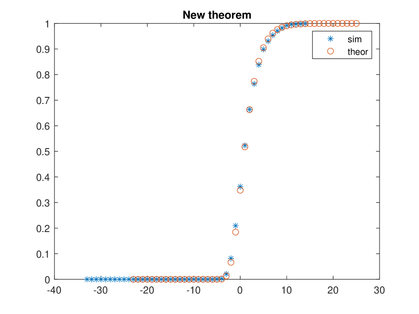
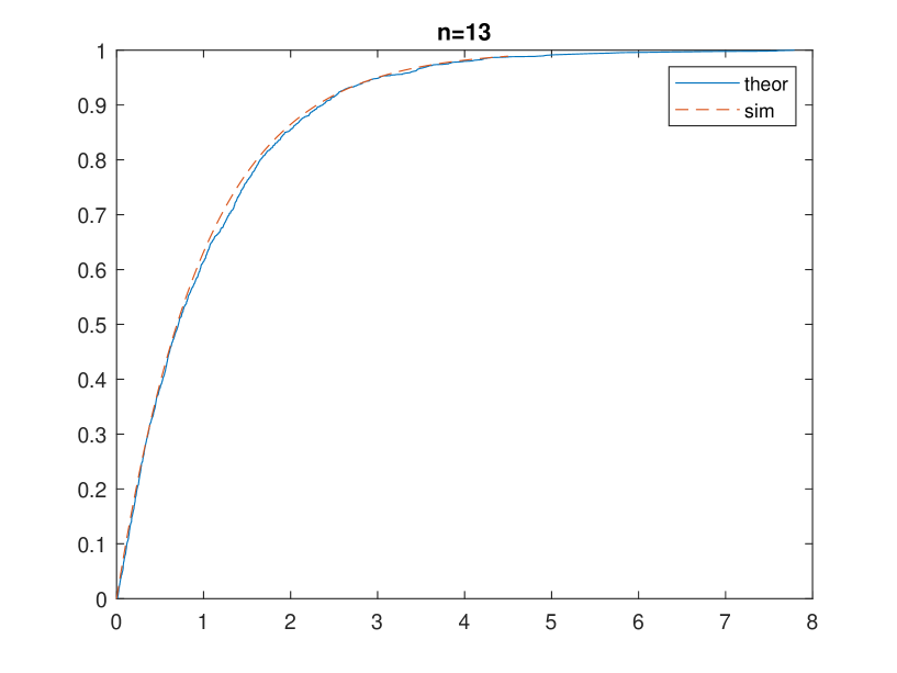
In this example p=0.5𝑝0.5p=0.5, T=1𝑇1T=1. The length of the coin tossing experiment is N=106𝑁superscript106N=10^{6}, the number of the repetitions of the experiment is s=2000𝑠2000s=2000. On parts (a) and (b) of Figure 1 sign oo{\rm{o}} shows the theoretical asymptotic probability and βˆ—βˆ—\ast shows the relative frequency of those experiments when μ​(N)πœ‡π‘\mu(N), that is the longest T𝑇T-contaminated run is shorter than the given value on the horizontal axis. Part (a) of Figure 1 shows the fit of the empirical distribution of μ​(N)πœ‡π‘\mu(N) to the asymptotic distribution given by our Theorem 2.2. The fit is good, the Kolmogorov distance is 0.02640.02640.0264. Part (b) of Figure 1 shows the fit of the empirical distribution of μ​(N)πœ‡π‘\mu(N) to the asymptotic distribution given by the old result quoted in Proposition 1.1. The fit is poor, the Kolmogorov distance is 0.07780.07780.0778. Part (c) of Figure 1 shows the first hitting time of the T𝑇T-contaminated run having length n=13𝑛13n=13. The solid line is the empirical distribution given by the simulation, the dashed line is the asymptotic theoretical distribution presented in Theorem 2.1. The fit is good.
Refer to caption
(a) Longest run (new)
Refer to caption
(b) Longest run (old)
Refer to caption
(c) First hitting time
Figure 1: T=1𝑇1T=1, p=0.5𝑝0.5p=0.5, N=106𝑁superscript106N=10^{6}, s=2000𝑠2000s=2000
Example 5.2.

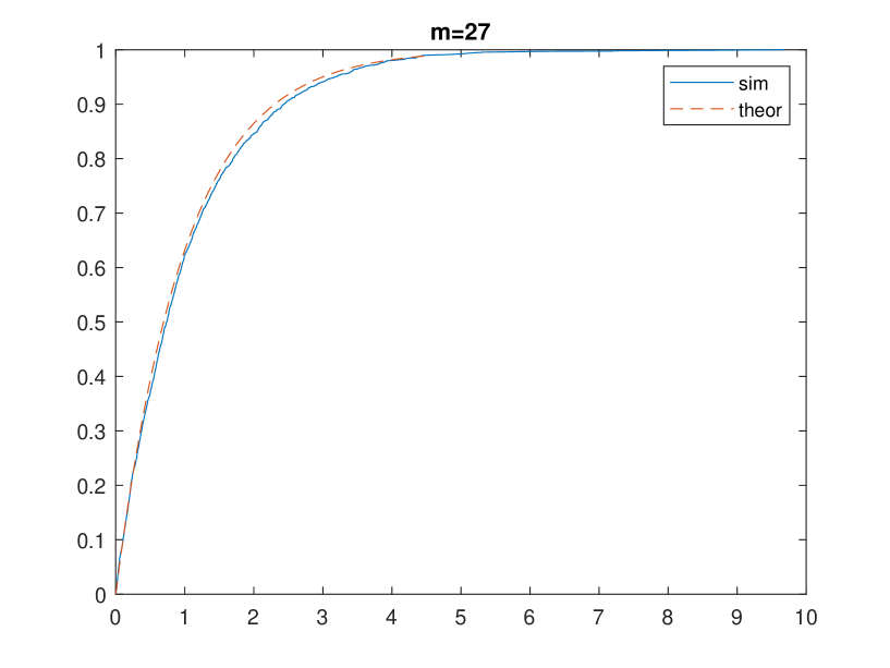
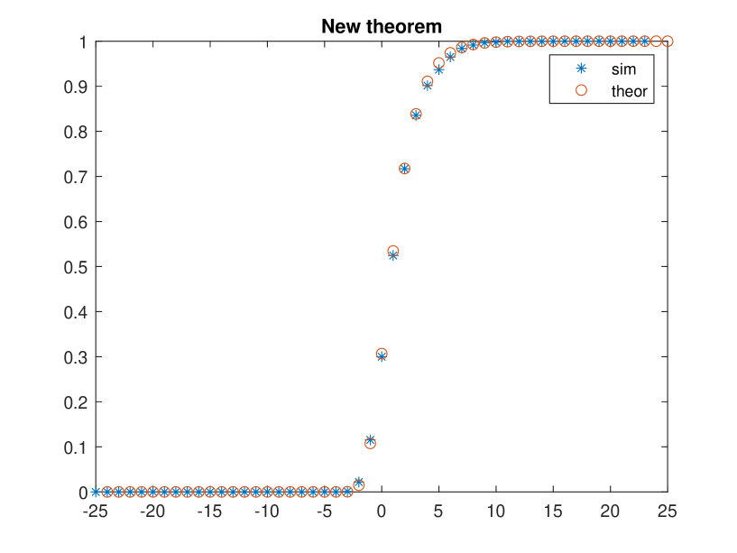
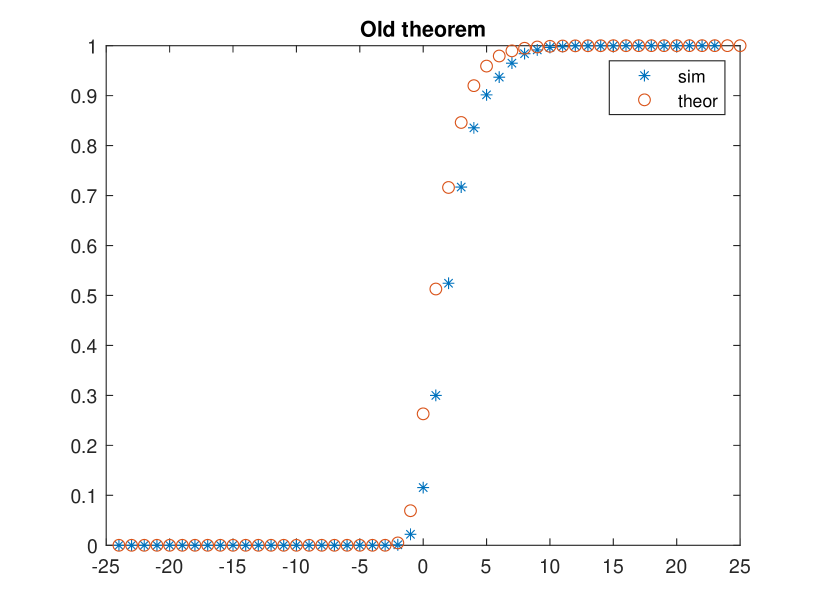
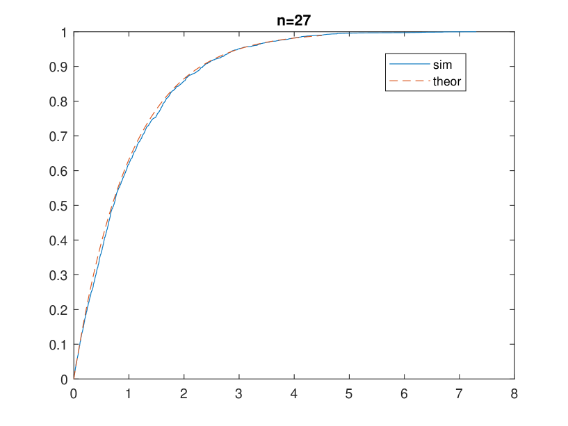
In this example p=0.5𝑝0.5p=0.5, T=2𝑇2T=2. The length of the coin tossing experiment is N=106𝑁superscript106N=10^{6}, the number of the repetitions of the experiment is s=2000𝑠2000s=2000. On parts (a) and (b) of Figure 2 sign oo{\rm{o}} shows the theoretical asymptotic probability and βˆ—βˆ—\ast shows the relative frequency of those experiments when μ​(N)πœ‡π‘\mu(N), that is the longest T𝑇T-contaminated run is shorter than the given value on the horizontal axis. Part (a) of Figure 2 shows the fit of the empirical distribution of μ​(N)πœ‡π‘\mu(N) to the asymptotic distribution given by our Theorem 2.2. The fit is good, the Kolmogorov distance is 0.01480.01480.0148. Part (b) of Figure 2 shows the fit of the empirical distribution of μ​(N)πœ‡π‘\mu(N) to the asymptotic distribution given by the old result quoted in Proposition 1.1. The fit is poor, the Kolmogorov distance is 0.21290.21290.2129. Part (c) of Figure 2 shows the first hitting time of the T𝑇T-contaminated run having length n=27𝑛27n=27. The solid line is the empirical distribution given by the simulation, the dashed line is the asymptotic theoretical distribution presented in Theorem 2.1. The fit is good.
Refer to caption
(a) Longest run (new)
Refer to caption
(b) Longest run (old)
Refer to caption
(c) First hitting time
Figure 2: T=2𝑇2T=2, p=0.5𝑝0.5p=0.5, N=106𝑁superscript106N=10^{6}, s=2000𝑠2000s=2000
Example 5.3.

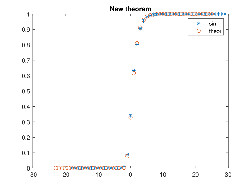
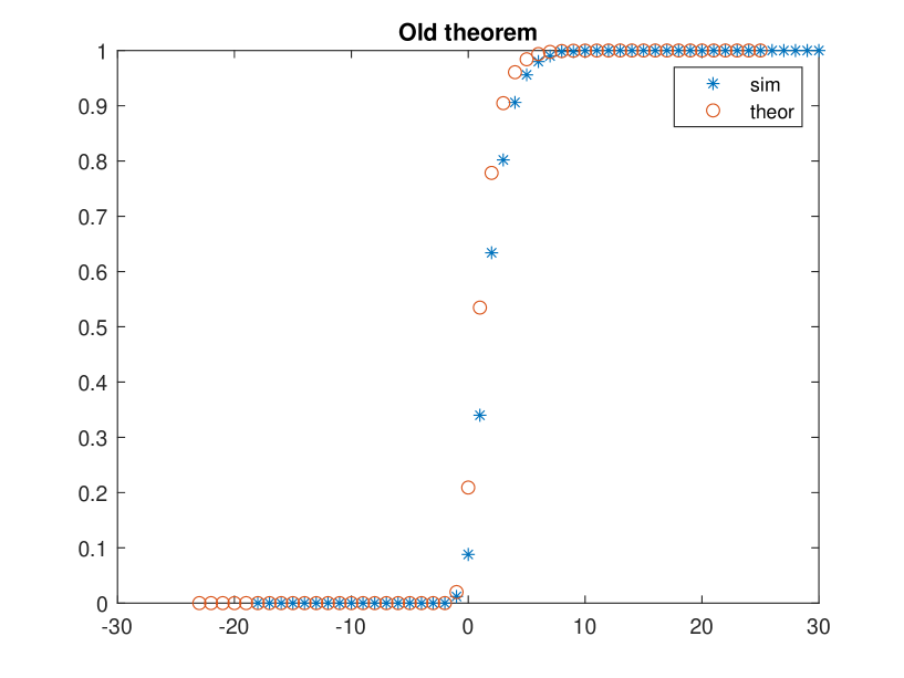
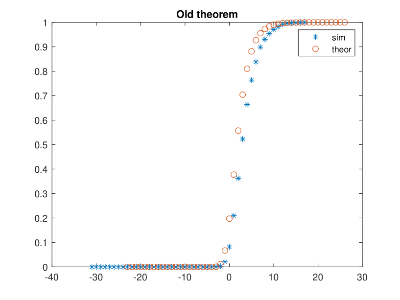
In this example p=0.6𝑝0.6p=0.6, T=2𝑇2T=2. The length of the coin tossing experiment is N=106𝑁superscript106N=10^{6}, the number of the repetitions of the experiment is s=2000𝑠2000s=2000. Part (a) of Figure 3 shows the fit of the empirical distribution of μ​(N)πœ‡π‘\mu(N) to the asymptotic distribution given by our Theorem 2.2. The fit is good, the Kolmogorov distance is 0.02500.02500.0250. Part (b) of Figure 3 shows the fit of the empirical distribution of μ​(N)πœ‡π‘\mu(N) to the asymptotic distribution given by the old result quoted in Proposition 1.1. The fit is poor, the Kolmogorov distance is 0.19530.19530.1953. Part (c) of Figure 4 shows the first hitting time of the T𝑇T-contaminated run having length n=27𝑛27n=27. The solid line is the empirical distribution given by the simulation, the dashed line is the asymptotic theoretical distribution presented in Theorem 2.1. The fit is good.
Refer to caption
(a) Longest run (new)
Refer to caption
(b) Longest run (old)
Refer to caption
(c) First hitting time
Figure 3: T=2𝑇2T=2, p=0.6𝑝0.6p=0.6, N=106𝑁superscript106N=10^{6}, s=2000𝑠2000s=2000
Example 5.4.

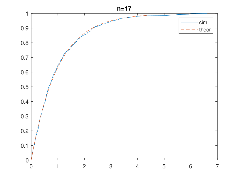
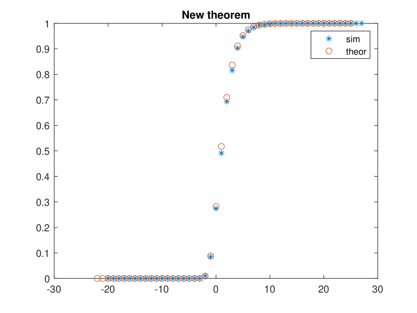
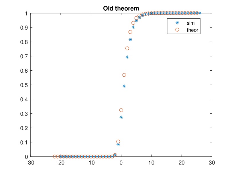
In this example p=0.4𝑝0.4p=0.4, T=2𝑇2T=2. The length of the coin tossing experiment is N=106𝑁superscript106N=10^{6}, the number of the repetitions of the experiment is s=500𝑠500s=500. Part (a) of Figure 4 shows the fit of the empirical distribution of μ​(N)πœ‡π‘\mu(N) to the asymptotic distribution given by our Theorem 2.2. The fit is good, the Kolmogorov distance is 0.01720.01720.0172. Part (b) of Figure 4 shows the fit of the empirical distribution of μ​(N)πœ‡π‘\mu(N) to the asymptotic distribution given by the old result quoted in Proposition 1.1. The fit is poor, the Kolmogorov distance is 0.19480.19480.1948. Part (c) of Figure 4 shows the first hitting time of the T𝑇T-contaminated run having length n=17𝑛17n=17. The solid line is the empirical distribution given by the simulation, the dashed line is the asymptotic theoretical distribution presented in Theorem 2.1. The fit is good.
Refer to caption
(a) Longest run (new)
Refer to caption
(b) Longest run (old)
Refer to caption
(c) First hitting time
Figure 4: T=2𝑇2T=2, p=0.4𝑝0.4p=0.4, N=106𝑁superscript106N=10^{6}, s=500𝑠500s=500

References

  • [1] CsΓ‘ki, E.; FΓΆldes, A.; KomlΓ³s, J. Limit theorems for ErdΕ‘s-RΓ©nyi type problems. Studia Sci. Math. Hungar. 22 (1987), 321–332.
  • [2] ErdΕ‘s, P.; RΓ©nyi, A. On a new law of large numbers, J. Analyse Math. 23 (1970), 103-111.
  • [3] ErdΕ‘s, P.; RΓ©vΓ©sz, P. On the length of the longest head-run. Topics in information theory (Second Colloq., Keszthely, 1975), pp. 219–228. Colloq. Math. Soc. JΓ‘nos Bolyai, Vol. 16, North-Holland, Amsterdam, 1977.
  • [4] Fazekas, I.; Ochieng Suja, M. Limit theorems for contaminated runs of heads. Annales Univ. Sci. Budapest., Sect. Comp. 52 (2021), 131–146.
  • [5] FΓΆldes, A. The limit distribution of the length of the longest head-run. Period. Math. Hungar. 10 (1979), no. 4, 301–310.
  • [6] Gordon, L.; Schilling, M. F.; Waterman, M. S. An extreme value theory for long head runs. Probab. Theory Relat. Fields 72 (1986), no. 2, 279–287.
  • [7] KomlΓ³s, J.; TusnΓ‘dy, G. On Sequences of ”Pure Heads”. Ann. Probab.3 (1975), no. 4, 608–617. DOI: 10.1214/aop/1176996304
  • [8] MΓ³ri, T. F. The a.s. limit distribution of the longest head run. Canad. J. Math. 45 (1993), no. 6, 1245–1262.
  • [9] Novak, S. Y. On the length of the longest head run. Statist. Probab. Lett. 130 (2017), 111–114.