Reinforcement Learning Aided Sequential Optimization for Unsignalized Intersection Management of Robot Traffic

Abstract

We consider the problem of optimal unsignalized intersection management for continual streams of randomly arriving robots. This problem involves repeatedly solving different instances of a mixed integer program, for which the computation time using a naive optimization algorithm scales exponentially with the number of robots and lanes. Hence, such an approach is not suitable for real-time implementation. In this paper, we propose a solution framework that combines learning and sequential optimization. In particular, we propose an algorithm for learning a shared policy that given the traffic state information, determines the crossing order of the robots. Then, we optimize the trajectories of the robots sequentially according to that crossing order. This approach inherently guarantees safety at all times. We validate the performance of this approach using extensive simulations. Our approach, on average, significantly outperforms the heuristics from the literature. We also show through simulations that the computation time for our approach scales linearly with the number of robots. We further implement the learnt policies on physical robots with a few modifications to the solution framework to address real-world challenges and establish its real-time implementability.

Note to Practitioners

The work is motivated towards combining reinforcement learning (RL) and optimization techniques for efficient real-time coordination in safety-critical multi-agent systems. Specifically, we choose to address the autonomous warehouse intersection management problem. Most of the works in this area, to have real-time algorithms, use some fixed heuristic to decide crossing order which is not directly involved in the process of trajectory optimization. This leads to inefficiencies. In our work, we let an RL agent learn a policy to decide efficient crossing order for arbitrary scenarios and optimization methods are used to obtain safe trajectories. Reward to the RL agent is directly related to the quality of the trajectories hence influencing the crossing order decisions. Results in the paper suggest that the proposed idea outperforms many heuristics. Future work involves extending the framework to multiple intersections and making the method robust to disturbances.

I Introduction

Unsignalized intersection management requires that a number of robots coordinate their trajectories for ensuring safe and efficient use of the intersection. This application is useful in contexts like automated warehouses with hundreds or thousands of mobile robots. The problem of optimal unsignalized intersection management inherently involves repeatedly solving mixed integer programs, for which the computational complexity of naive optimization methods scales very badly with the number of robots and lanes. As a result, they are not suitable for real-time implementation. In this work, we propose a learning based solution framework to get near-optimal solutions in real-time.

I-A Related work

Unsignalized intersection management for robots or connected and automated vehicles has been studied using different methods and tools over the years. Surveys in [1], [2] and [3] give a detailed description of the recent literature. Here we focus on the optimal unsignalized intersection management problem, which is a very common formulation in the area. While some formulate this problem as a mixed integer linear program [4, 5, 6, 7], others consider a model predictive control approach [8] and some formulate a non-linear problem and use genetic algorithms to solve it [9, 10]. While typically the optimization goal is to minimize the cumulative travel times or maximize the cumulative distance covered by all the robots, recent works like [11, 12, 13] also take energy consumption into account while computing the optimal trajectories. Works like [14, 15] discretize the space and use $A^{*}$ like algorithms to get collision free optimal trajectories for the participating agents.

As naive or generic optimization methods for these problems scale very badly with the number of robots and lanes, there is also interest in developing computationally simpler solution methods. With this motivation,  [16, 17, 18] propose solutions that cluster the vehicles/robots in order to reduce the computational or communication effort. To address computational complexity, works like [19] describe general ideas of prioritized motion planning for coordination among multiple agents, but, assuming the knowledge of some pre-assigned priorities to each agent. Similarly, in line with prioritized planning idea, some other works, such as [20, 5] use model based heuristics to decide the crossing order and solve centralized/decentralized optimization problems preserving that order to get the trajectories for involved robots in an intersection. Work [21] uses a similar approach for the ramp merging problem. While some works like [22, 23] consider finding optimal and safe trajectories to robots assuming a priority (e.g. first-in first-out) rule, some like [24, 25] propose an optimization problem to get such priority rule and solve another optimization problem (in receding horizon control framework) to get trajectories. Other approaches to the problem include auction based methods [26, 27] and first come first serve based reservation of regions against time [15]. Work in [27] proposes a game-theoretic social-welfare optimal auction strategy to decide the crossing order. Others [8, 28] construct/use a priority graph to get feasible solutions and conflict resolution. Work [13] uses similar approach to the intersection management problem and computes the priority/crossing order using a set of features associated with the robots. Then the robots solve an optimal control problem sequentially to obtain their trajectories.

The current literature on the use of learning methods for intersection management includes [29, 30, 31, 32, 33, 34, 35]. These papers consider only a first order kinematic model for the robots and the learnt policy gives the position trajectories of the robots. [36] proposes a learning based solution for optimizing robots’ trajectories under bounded deviations of other robots from some nominal trajectories. In other multi-robot applications, there are works like [37, 38] that learn path planning policies for navigation through narrow passages or hallways. Other works such as [39] present RL algorithms for general multi-robot trajectory coordination for purely first order kinematic robots. The core idea of our work has similarities to [40, 41, 42, 43], which use RL methods to improve the efficiency of solving a parametrized combinatorial or mixed-integer optimization problem, for which the parameters are revealed online.

One of the main applications of our work is collision free warehouse automation. Prioritized/sequential planning seems to be a popular approach since it is both scalable and gives near-optimal solutions. Some works like [19, 44, 45, 46, 47] assume the knowledge of some priorities over agents negotiating a path conflict (at an intersection), while [48] uses first come first serve policy for conflict resolution.

I-B Contributions

The following are the main contributions of this paper.

• We present a solution framework that combines learning and online optimization for unsignalized intersection management of a continual stream of robot traffic. The framework implicitly guarantees safety at all times, both during training and deployment.

• We propose an algorithm for learning a policy for determining the crossing order of the robots, given certain features of the traffic. The algorithm learns a policy that is shared among all the robots.

• Through extensive simulations, we establish that the proposed framework solves the intersection management problem in real-time and provides near-optimal solutions. In general, the performance of the trained policies is significantly superior compared to many heuristics from the literature.

• We propose some adaptations to the underlying solution framework to address real-world implementation challenges like tracking errors and delays associated with communication and computation. The framework with these adaptations is deployed on physical robots to establish the real-time implementability of the framework.

For computational scalability, several works decide the crossing/planning sequence (scheduling) among the robots and then get their trajectories by solving optimization problems in that order (prioritized/sequential planning). Scheduling is done using various techniques like auctions [26], job scheduling mechanisms [17] or some heuristics [5, 20, 21, 27]. The problem with this approach is that scheduling is dissociated from the trajectory generation and may lead to sub-optimal trajectories. Moreover, optimal policy for scheduling may be highly dependent on the type of intersection and other settings. Our past work [13] has a similar solution framework as in this paper. However, [13] contains no method or learning algorithm for obtaining a policy for determining crossing orders.

To the best of our knowledge, there are very few works like [49, 24, 25] which makes a systematic attempt at assigning priorities to the involved agents. Existing approaches to find a good set of priorities include iterative search algorithms [49] or solving an optimization problem [24, 25] which in itself are time consuming.

Although [29, 30, 31] use RL to directly generate trajectories of the robots, the approach inherently cannot guarantee safety in a deterministic way. Further, these works only consider first order kinematic models of the robots, whereas we consider a double integrator model for the robots. Our proposed approach is very similar in spirit to [40, 41, 42, 43], which use learning methods to solve combinatorial optimization problems. However, these papers are for very different applications. Additionally, all these works provide algorithms that learn policies for a single agent rather than multiple agents.

II Unsignalized Intersection Management and Problem setup

Figure 1: A schematic of an example intersection and the region of interest (RoI) with 8 lanes.

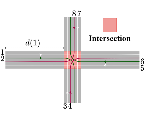
In this section, we first present the unsignalized intersection management problem and discuss some challenges in solving it in real-time. Then, we pose a problem of learning computationally efficient and near-optimal policies that can be utilized for safe intersection management in real-time. We first describe the intersection geometry, robots and notation.

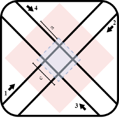
We consider an isolated region of interest (RoI) consisting of fixed lanes - leading to, going through and leaving an unsignalized intersection. Figure 1 shows one such example configuration. The lanes intersect only inside the intersection.

We assume that the robots travel only along the fixed lanes inside the RoI, i.e., they do not change lanes. We denote the set of robots under consideration by $V$. We denote the length of robot $i\in V$ with $L_{i}$. Further for a robot $i\in V$, we denote its time of arrival into the RoI, time of entry into and time of exit from the intersection by $t^{\mathcal{A}}_{i}$, $t^{\mathcal{E}}_{i}$ and $t^{\mathcal{X}}_{i}$, respectively. The time of arrival of a robot into the RoI is unknown before its arrival. We use $x_{i}(t)$, $v_{i}(t)$ and $u_{i}(t)$ to denote the longitudinal position (specifically, front end of the robot), longitudinal velocity and longitudinal acceleration of the robot, respectively, along its lane $q_{i}$ at time $t\geq 0$. For a lane $l$, we denote its length of approach to the intersection as $d(l)$. On each lane, we set up the coordinates such that for a robot $i\in V$ we have, $x_{i}(t^{\mathcal{A}}_{i})=-d(q_{i})$ and $x_{i}(t^{\mathcal{E}}_{i})=0$.

We assume that the robots follow the double integrator dynamics with longitudinal acceleration as their input, i.e.,

$$\dot{x}_{i}(t)=v_{i}(t)\ ,\ \dot{v}_{i}(t)=u_{i}(t),\ \forall i\in V,\ t\geq t^{\mathcal{A}}_{i}.$$ (1)

We assume that the robots’ velocities and accelerations are bounded, i.e.,

$$v_{i}(t)\in[0,\bar{v}_{i}]\ \mathrm{and}\ u_{i}(t)\in[\underline{u},\bar{u}],\ \forall i\in V,\ \forall t\geq t^{\mathcal{A}}_{i}.$$ (2)

We suppose that $\underline{u}<0$. To avoid collisions between robots $i,j\in V$ travelling on the same lane and $i$ following $j$, we impose the constraints

$$x_{j}(t)-x_{i}(t) \geq L_{j}+\max\left(0,\frac{v_{j}(t)^{2}-v_{i}(t)^{2}}{2\underline{u}}\right),\ \forall t\geq t^{\mathcal{A}}_{i},$$

$$\forall i,j\in V, \ \mathrm{s.t.}\ q_{i}=q_{j}\ \mathrm{and}\ x_{i}(t)<x_{j}(t).$$ (3)

To avoid collisions inside the intersection between robots on a pair of conflicting or incompatible lanes (pairs of lanes which intersect), we impose the constraint

$$t^{\mathcal{E}}_{i}\geq t^{\mathcal{X}}_{j}\ \mathrm{OR}\ t^{\mathcal{E}}_{j}\geq t^{\mathcal{X}}_{i},\ \forall i,j\in V,\text{ if }q_{i}\text{ and }q_{j}\text{ intersect}.$$ (4)

Note that the constraint (4) is combinatorial.

Remark 1.

(Rear end safety constraint). In situations like ware-houses, there is always a chance of robot or communication failure. Further, the environment is dynamic and there may be chances of some unplanned obstacles coming in the path (lanes) of the robots. Hence we propose a conservative rear end safety constraint (3), which ensures the existence, at all times, of a feasible input (acceleration) trajectory for a robot to come to a stop, avoiding collision, irrespective of the trajectory taken by the robot ahead [50]. $\bullet$

Control objective

We formulate the intersection management problem as the optimal control problem (5) and seek optimal trajectories for the robots in $V$, which enter the RoI at different time instants during a time interval of interest.

$$\begin{split}&\underset{u_{i}(.),\ \forall i\in V}{\max}\sum_{i\in V}r_{i}\int\displaylimits_{t^{\mathcal{A}}_{i}}^{t^{\mathcal{A}}_{i}+T_{h}}\ v_{i}(t)\mathrm{d}t\\ &\mathrm{s.t.}\ \eqref{eq:dynamics},\eqref{eq:vel_acc_bounds},\eqref{eq:c0_rear_end_safety},\forall t\in[t^{\mathcal{A}}_{i},t^{\mathcal{A}}_{i}+T_{h}],\ \eqref{eq:intersection_safety}.\end{split}$$ (5)

Here $T_{h}$ is a sufficiently long time horizon and $r_{i}>0$ is a weight indicating the priority for robot $i$. We assume that the arrival time, $t^{\mathcal{A}}_{i}$, of a robot $i\in V$ is random and is unknown before its arrival. Problem (5) is a proxy for minimizing the average travel times of the robots $V$ through the intersection. We use the formulation (5) as it has the advantage of a fixed time horizon $T_{h}$ for each robot.

Remark 2.

(Challenges in solving Problem (5) directly). There are several challenges in solving Problem (5). They mainly stem from the following factors.

1. At any given time instant, the exact information about the future arrival of robots is not available.

2. Constraint (4) is combinatorial, which makes Problem (5) a mixed integer program. A naive optimization approach scales exponentially with the number of robots and lanes. This is problematic because intersection management problem is both time and safety critical.

In order to counter these challenges, we use a data-driven approach similar to the one in [13], wherein data obtained through simulations was used to manually tune the policy. In the current work, we propose algorithms that learn near-optimal policies to Problem (5). $\bullet$

Informal problem statement

In this work, we seek to develop algorithms that learn near-optimal policies for Problem (5). While we allow the learning to be centralized, implementation of learnt policies should be distributed, i.e., the policy for each robot should depend on only the data that can be easily obtained using robot-to-robot and robot-to-infrastructure communication. The proposed solution should be applicable to a continual stream of robots arriving randomly into the RoI. Note that any feasible solution to Problem (5) implicitly guarantees safety.

III Solution framework to address random arrival times

In this section, we present an overall framework/algorithm for solving the intersection management problem. The broad solution framework is a modified version of the one in [13]. We recap the main aspects of this framework.

As the arrival times of robots are unknown beforehand and coordination between robots requires planning for groups of robots at a time, we split the trajectory of each robot into two phases - provisional phase and coordination phase. Provisional phase of a robot begins when it arrives at the RoI and ends when its coordination phase begins. A coordination phase algorithm runs every $T_{c}$ seconds and assigns safe and efficient trajectories for crossing the intersection to the robots in their provisional phase.

Before we discuss the specifics of this framework, we introduce some notation. For a robot $i\in V$, $t^{\mathcal{C}}_{i}\geq t^{\mathcal{A}}_{i}$ represents the time at which its coordinated phase starts, and hence $t^{\mathcal{C}}_{i}=kT_{c}$ for some $k\in\{1,2,...\}$. We let $V(k):=\{i\in V:t^{\mathcal{A}}_{i}<kT_{c}\}$ be the set of robots which entered the RoI before $kT_{c}$, $V_{s}(k):=\{i\in V(k):t^{\mathcal{C}}_{i}<kT_{c}\}$ be the robots that entered coordinated phase before $kT_{c}$, $V_{p}(k):=V(k)\setminus V_{s}(k)$, i.e., the set of robots that need coordinated phase trajectories at $kT_{c}$.

III-A Provisional phase

Consider a robot $i\in V_{p}(k)$ ($k\in\mathbb{N}$). To ensure that the robot does not enter the intersection before it enters the coordinated phase, we impose the constraint

$$v_{i}(t)\leq\sqrt{2\underline{u}_{i}x_{i}(t)}.$$ (6)

We let the robot’s acceleration input for the provisional phase trajectory in the time interval $[\max\{t^{\mathcal{A}}_{i},(k-1)T_{c}\},kT_{c}]$ be an optimal solution of the following problem.

$$\begin{split}&\underset{u_{i}(.)}{\max}\int\displaylimits_{\max\{t^{\mathcal{A}}_{i},(k-1)T_{c}\}}^{kT_{c}}\ v_{i}(t)\mathrm{d}t\\ &\mathrm{s.t.}\ \eqref{eq:dynamics},\eqref{eq:vel_acc_bounds},\eqref{eq:c0_rear_end_safety},\eqref{eq:prov_int_safety},\ \forall t\in[\max\{t^{\mathcal{A}}_{i},(k-1)T_{c}\},kT_{c}].\end{split}$$ (7)

III-B Coordinated phase

At the time $kT_{c}$, for each $k\in{\mathbb{N}}$, some or all the robots in $V_{p}(k)$ are assigned their coordinated phase trajectories, which they start executing immediately. Ideally, we would like the coordinated phase control input trajectories for the robots in $V_{p}(k)$ to be an optimal solution of Problem (8), which we call as the combined optimization problem.

$$\begin{split}&\underset{u_{i}(.)\forall i\in V_{p}(k)}{\max}\sum_{i\in V_{p}(k)}r_{i}\int\displaylimits_{kT_{c}}^{kT_{c}+T_{h}}v_{i}(t)\mathrm{d}t\\ &\mathrm{s.t.}\ \eqref{eq:dynamics},\eqref{eq:vel_acc_bounds},\eqref{eq:c0_rear_end_safety},\ \forall t\in[kT_{c},kT_{c}+T_{h}],\ \eqref{eq:intersection_safety}.\end{split}$$ (8)

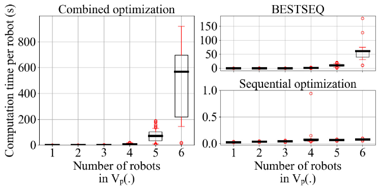
Note that the robots in $V_{s}(k)$ would also appear in the constraints of Problem (8). Intersection safety constraint in Problem (8) is still combinatorial. Solving Problem (8) involves picking a feasible solution with highest objective value among all the feasible crossing orders. As a result, this formulation scales exponentially with the number of robots and is not suitable for real-time implementation. We illustrate this exponential scaling of computation times through simulations in Figure 2.

Remark 3.

(Possibility of multiple provisional phases for a robot). In busy intersections, there might be cases where the solution to Problem (8) gives a trajectory for a robot $i\in V_{p}(k)$ such that the robot does not exit the intersection by $kT_{c}+T_{h}$. This can potentially cause infeasibility of Problem (8) in subsequent coordinated phases. In order to avoid such a situation, such affected robots (robot $i$ and its successors in the crossing order) go through the provisional phase again for the interval $[kT_{c},(k+1)T_{c})$. This is the reason for why the time horizon for robot $i\in V_{p}(k)$ is $[\max\{t^{\mathcal{A}}_{i},(k-1)T_{c}\},kT_{c}]$ in Problem (7). $\bullet$

Sequential optimization for coordinated phase

To address non-scalability of combined optimization for obtaining coordinated phase trajectories, we present a modified version of sequential optimization from [13] in Algorithm 1. The algorithm takes as input a set of quantities called precedence indices $(p_{i}\in\mathbb{R},\ \forall i\in V_{p}(k))$, which determine the crossing order. Each robot in $V_{p}(k)$ obtains its coordinated phase trajectory sequentially, as per the crossing order, by solving the optimization problem in (9).

3 $V_{Q}=V_{p}(k)$

4 while $|V_{Q}|>0$ do

5       $\mathcal{F}\leftarrow\{i\in V_{Q}:x_{i}\geq x_{j},\ \forall j\in V_{Q}\ \texttt{s.t.}\ q_{i}=q_{j}\}$

6      

7      $\displaystyle i^{*}\leftarrow\operatorname*{argmax}_{\{j\in\mathcal{F}\}}\ \{p_{j}\}$

8       $V_{s}^{i^{*}}\leftarrow V_{s}(k)\cup(V_{p}(k)\setminus V_{Q})$

9       $u_{i^{*}}(.)$ $\leftarrow$ Solve (9) for robot $i^{*}$

10      

11      if $i^{*}$ crosses the intersection by time $kT_{c}+T_{h}$ with $u_{i^{*}}(.)$,  then

12             $t^{\mathcal{C}}_{i^{*}}\leftarrow kT_{c}$

13             $i^{*}$ starts executing $u_{i}^{*}$ at $t^{\mathcal{C}}_{i^{*}}$

14             Remove $i^{*}$ from $V_{Q}$

15       end if

16      

17      else

18             Break out of while loop

19       end if

20      

21 end while

22

Inputs: $V_{p}(k)$, $V_{s}(k)$, $p_{i}\ \forall i\in V_{p}(k)$

Algorithm 1 sequential_optimization

Inputs: $V_{p}(k)$, $V_{s}(k)$, $p_{i}\ \forall i\in V_{p}(k)$

In Algorithm 1, at the beginning of each iteration of the while loop, $V_{Q}$ is the subset of robots in $V_{p}(k)$ that do not have a coordinated phase trajectory yet. In Step 3, $\mathcal{F}$ is the set of robots in $V_{Q}$ that are nearest to the intersection in their respective lanes. In Step 4, we obtain the robot $i^{*}$ in $\mathcal{F}$ with the largest precedence index $p_{i^{*}}$, after breaking ties arbitrarily. In Step 5, $V_{s}^{i^{*}}$ is the set of all robots that were assigned a coordinated phase trajectory before the robot $i^{*}$. If $u_{i}^{*}(.)$, computed in Step 6, enables the robot to cross the intersection before $kT_{c}+T_{h}$, then the robot $i^{*}$ starts executing $u_{i}^{*}(.)$ as its coordinated phase control trajectory, starting at $t^{\mathcal{C}}_{i^{*}}=kT_{c}$. Then, $i^{*}$ is removed from $V_{Q}$ and the loop continues. On the other hand, if $i^{*}$ cannot cross the intersection with the control trajectory $u_{i^{*}}(.)$ then we break out of the loop and $i^{*}$ and the rest of the robots in $V_{Q}$ go through another provisional phase, as described in Remark 3.

In Step 6 of Algorithm 1, $u_{i^{*}}(.)$ is obtained by solving the following optimization problem.

$$\begin{split}&J_{i^{*}}^{*}=\underset{u_{i^{*}}(.)}{\max}\int\displaylimits_{kT_{c}}^{kT_{c}+T_{h}}v_{i^{*}}(t)\mathrm{d}t\\ &\mathrm{s.t.}\ \eqref{eq:dynamics},\eqref{eq:vel_acc_bounds},\eqref{eq:c0_rear_end_safety},\ \forall t\in[kT_{c},kT_{c}+T_{h}],\ \mathrm{with}\ i=i^{*},\\ &\text{and }t^{\mathcal{E}}_{i^{*}}\geq\tau_{i^{*}},\end{split}$$ (9)

where $\tau_{i^{*}}$ is the minimum wait time of $i^{*}\in V_{p}(k)$, given by,

$$\tau_{i^{*}} =\max\{t^{\mathcal{X}}_{m}\ :\ m\in V_{s}^{i^{*}}\ \text{s.t. }q_{i^{*}}\text{ and }q_{m}\text{ intersect}\}.$$

Remark 4.

(Features of Algorithm 1). Algorithm 1 has several good features, which help in achieving the design goals of scalability and real-time implementation. In a variety of simulations, we have consistently observed that the computation for Algorithm 1 scales linearly with the number of robots. We illustrate this feature in Figure 2. Algorithm 1 is an efficient version of the DD-SWA algorithm proposed in [13], as the precedence indices need not be recomputed after the trajectory optimization for each robot. The solution framework, including Algorithm 1, can be implemented in a distributed manner. Reader may refer to relevant discussions in [13]. $\bullet$

For the solution framework to be complete, we still need to specify how the precedence indices $p_{i}$ are to be chosen. In the next section, we propose an algorithm for learning a policy that gives out “near-optimal” precedence indices, given some information about the traffic state.

IV Learning a policy that gives near-optimal crossing orders

Recall that at $kT_{c}$, the beginning of the $k^{\text{th}}$ coordinated phase, $V_{p}(k)$ is the set of robots that need coordinated phase trajectories and $V_{s}(k)$ is the set of robots that are already executing their coordinated phase trajectories. Notice that Algorithm 1 takes as input the precedence indices of the robots in $V_{p}(k)$, using which it sequentially optimizes the coordinated phase trajectories of the robots. In this section, we are interested in obtaining a policy that determines the precedence indices of the robots in $V_{p}(k)$, given the traffic state, so that Algorithm 1 provides optimal or at least near-optimal solutions to the combined optimization problem (8) and more generally to the original optimization problem (5).

In particular, we propose a centralized algorithm for learning a policy, which

1. can be implemented online in real-time.

2. is shared, i.e., the same policy is used by all the robots.

3. is distributed, i.e., a policy to which the inputs are information available to a robot locally or through communication with its neighboring robots.

4. can be implemented on an arbitrary number of robots.

We denote the shared policy by the function $g(.)$. For robot $i$, the input to the policy is the feature vector, $f_{i}$, that captures the state of the traffic relevant to robot $i$. Then, the precedence indices are

$$p_{i}=g(f_{i}),\quad\forall i\in V_{p}(k).$$ (10)

There may be different number of robots in $V_{p}(k)$ for different $k\in{\mathbb{N}}$. However, given the dimensions of the RoI and lengths of the robots we can determine $N_{r}$, an upper bound on the number of robots that could ever be in $V_{p}(k)$. Then, we pad the set of robots in $V_{p}(k)$ with $N_{r}-|V_{p}(k)|$ number of pseudo robots so that the state and action space dimensions remain constant for each $k\in{\mathbb{N}}$. Pseudo robots are virtual robots with features chosen such that they do not affect the feasibility and optimality of the crossing order and trajectories of the real robots. For e.g., the position of a pseudo robots can be picked far away from entry to RoI.

Let $\tilde{V}(k)$ be the union of $V_{p}(k)$ and the set of pseudo robots, so that $|\tilde{V}(k)|=N_{r}$. Then, consider the Markov decision process (MDP) with the state, action, reward and the next state at the $k^{\text{th}}$ iteration defined as follows.

1. The state, $s$, is the vector formed by concatenated feature vectors of all the robots in $\tilde{V}(k)$.

2. The action, $a$, is the vector of precedence indices of all the robots in $\tilde{V}(k)$.

3. The reward, $R$, is as given in (11).

4. The next state, $s^{\prime}$, is the concatenated feature vectors of the robots in $\tilde{V}(k+1)$.

Remark 5.

(Reward function). Consider the $k^{\text{th}}$ coordinated phase. Given the action $a$ (precedence indices), let

$$V_{c}(k):=\{i\in V_{p}(k):t^{\mathcal{C}}_{i}=kT_{c}\},\ V_{nc}(k):=V_{p}(k)\setminus V_{c}(k),$$

where $t^{\mathcal{C}}_{i}$ is the time at which robot $i$ begins its coordinated phase, according to Algorithm 1. Thus, $V_{c}(k)$ is the set of robots that begin their coordinated phase at $kT_{c}$, while the robots in $V_{nc}(k)$ undergo another provisional phase. Then the reward function is

$$\begin{split}R=&\sum_{i\in V_{c}(k)}r_{i}\frac{x_{i}(t^{\mathcal{A}}_{i}+T_{r})-x_{i}(t^{\mathcal{A}}_{i})}{|V_{p}(k)|}\\ &-\sum_{j\in V_{nc}(k)}\bar{r}\frac{(d(q_{j})-x_{j}(kT_{c}))^{2}}{|V_{p}(k)|},\end{split}$$ (11)

where $T_{r}$ is a suitable time horizon for the computation of the reward and $\displaystyle\bar{r}=\max_{i\in V}r_{i}$ is the maximum priority among all the the considered robots. The first term is the weighted sum of distances covered by the robots in $V_{c}(k)$ during a time interval of length $T_{r}$ since their arrival into RoI. As Algorithm 1 does not provide a coordinated phase trajectory for the robots in $V_{nc}(k)$, for each robot in $V_{nc}(k)$, we have a penalty term proportional to the square of the distance covered by the robot from its time of arrival up to $kT_{c}$. This penalty helps in learning a near-optimal precedence index policy (10). We observed that penalizing all the robots with the equal weight of $\bar{r}$ (in contrast to weighing penalty terms by individual priorities) leads to better policies. This may be due to the reason that a low priority robot crossing quickly makes way for a higher priority robot which will arrive in the future to travel quickly. $\bullet$

Multi-Agent Joint-Action DDPG (MAJA-DDPG)

We use a modified version of the centralized multi-agent Deep Deterministic Policy Gradient (MA-DDPG [51]) algorithm to learn the precedence index policy (10). In this framework, the shared policy $g(.)$ is encoded by an actor neural network. In addition, there are neural networks encoding a target actor, a critic network encoding the estimated action value function $Q(.)$ and a target critic network $\hat{Q}(.)$. Let $\theta$, $\hat{\theta}$, $\phi$ and $\hat{\phi}$ be the parameters of the actor, target actor, critic and target critic networks, respectively. We store the (joint-state, joint-action, reward and joint-next-state) tuples in the replay buffer and use samples from this replay buffer to update the central-critic and shared actor networks in each learning iteration.

Suppose that $(s_{m},a_{m},R_{m},s^{\prime}_{m})$ is the $m^{\text{th}}$ sampled tuple out of $N$ samples. The critic is updated to minimize the loss function $E$, given in (12). The actor is updated according to “gradient” ascent of the sampled gradient of estimated return $J$ with respect to actor parameters $\theta$, as in (13).

$$E=\frac{1}{N}\sum_{m}{(R_{m}+\gamma\hat{Q}(s^{\prime}_{m},\hat{G}(s^{\prime}_{m}))-Q(s_{m},a_{m}))^{2}}.$$ (12)

$$\nabla_{\theta}J=\frac{1}{N}\sum_{m}{\nabla_{a}Q(s,a)|_{s=s_{m},a=G(s_{m})}\nabla_{\theta}G(s)|_{s=s_{m}}}.$$ (13)

Here $G(s)$ and $\hat{G}(s)$ represent the joint action (concatenated precedence indices of all robots in $V_{p}(k)$) and joint target action of all the robots in $V_{p}(k)$, respectively. Rest of the updates for target networks are similar to what is followed in the DDPG algorithm in [52].

Online and offline learning approaches

Algorithm 2 is the online approach to the proposed learning algorithm. We generate streams of robots using a poisson process for determining the arrival times of robots and choosing their initial velocities randomly. All these robots go through provisional and coordinated phases as described in Section III, where Algorithm 1 is used for obtaining coordinated phase trajectories. Since in Algorithm 1, we only care about the relative order of the precedence indices, we have a softmax layer as the last layer in the RL actor network and use these values as the precedence indices of corresponding robots. We observed that having this layer leads to quicker learning. We add the corresponding state, action, reward and next state tuple to the replay buffer and update the critic, actor and the target networks as described above. Note that because of the softmax layer, the implementation of this algorithm cannot be done in a truly distributed manner. We use a modified Ornstein-Uhlenbeck process (with decaying variance in added Gaussian noise) as the exploration noise. Algorithm 2 can be run in an online loop continuously, gathering data and learning from it.

3 $\tilde{V}(k)\leftarrow V_{p}(k)\cup\texttt{pseudo robots}$

4 s $\leftarrow$ concatenated feature vectors of robots in $\tilde{V}(k)$

5 $P\leftarrow\big{(}g(f_{j})\big{)}_{j=1}^{j=|\tilde{V}|}$

6 $a$ $\leftarrow$ softmax($P$) + exploration_noise

7 sequential_optimization ($V_{p}(k)$, $V_{s}(k)$, $\{a_{j}:j\in V_{p}(k)\}$)

8 Compute reward $R$ according to (11)

9 $s^{\prime}$ $\leftarrow$ concatenated feature vectors of robots in $\tilde{V}(k+1)$

10 Add $(s,a,R,s^{\prime})$ tuple to replay-buffer Update $g$ and $Q$ as in  [52] using (12) and (13)

11 Update targets $\hat{g}$ and $\hat{Q}$ using a polyak factor as in [52]

Return replay-buffer, $g$

Inputs: $V_{p}(k)$, $V_{s}(k)$, shared-policy $g$, replay-buffer

Algorithm 2 online_learning

Inputs: $V_{p}(k)$, $V_{s}(k)$, shared-policy $g$, replay-buffer

Similar to DDPG and MADDPG, the proposed algorithm can also be used for offline learning. Given a data-rich replay buffer, the mini-batches can be sampled from this replay buffer and the RL agent’s actor and critic networks can be updated iteratively. We propose an offline learning approach which involves constructing multiple individual replay buffers, one for each average arrival rate of robots using the steps as indicated in the online-approach and then merging them to form a new merged replay buffer. This merged replay buffer is then used to train a common policy, which can then be deployed for a range of average arrival rates. We refer to this as the Collect-Merge-Learn (CML) approach.

Remark 6.

(Differences between DDPG [52], MADDPG [51] and MAJA-DDPG). While DDPG, MADDPG and MAJA-DDPG are all centralized learning algorithms, DDPG learns a policy for a single agent. Both MADDPG and MAJA-DDPG learn a shared policy for multiple agents. The main difference between MADDPG and our proposed MAJA-DDPG is in the computation of the sampled gradient of $J$ in (13). MAJA-DDPG uses the gradient of the critic action value function $Q$ with respect to the shared actor parameters $\theta$ through the joint action (concatenated actions of all the agents), whereas MADDPG estimates the gradient of $Q$ with respect to the shared actor parameters $\theta$ through the action of a randomly selected agent in the corresponding computation. $\bullet$

Remark 7.

(List of features of a robot). We consider the following quantities as features of a robot $i\in V_{p}(k)$: its distance from the entry to RoI ($x_{i}(kT_{c})-d(q_{i})$), its current velocity ($v_{i}(kT_{c})$), its priority ($r_{i}$), its lane identifier ($q_{i}$), upper-bound on its velocity ($\bar{v}_{i}$), upper-bound on acceleration ($\bar{u}$), time since its arrival into RoI ($kT_{c}-t^{\mathcal{A}}_{i}$), its estimated minimum wait time ($\bar{\tau}_{i}=\max\{t^{\mathcal{X}}_{j}:j\in V_{s}(k)\}$) the number of robots following on its lane, and the average distance between the robots following it on its lane. As can be seen, most of these features can be directly measured or computed by robot $i$, whereas the others can be obtained by communicating with neighbouring robots. $\bullet$

V Simulation results

In this section, we present simulations comparing the proposed learning based sequential optimization algorithm against combined optimization and some other policies from literature.

V-A Simulation setup

Simulation parameters

We consider a warehouse scenario with $8$ lanes meeting in the intersection from 4 directions. Each lane has an approach length of $7m$, i.e., $d(l)=7$m, $\forall l\in\{1,2,...,8\}$ in Figure 1. Each lane is $0.7m$ wide, making the intersection a square of side $2.8m$. For each robot $i$, its length $L_{i}$ is $0.75m$ and upper and lower bounds on its acceleration are $2m/s^{2}$ and $-2m/s^{2}$, respectively. The initial velocity of robot $i$ is sampled from a uniform distribution on $[0,\bar{v}_{i}]$. We carried out simulations for streams of randomly arriving robots with various average arrival rates. In particular, streams were generated by choosing tentative arrival times of robots into the lanes according to a poisson process, with a specified average arrival rate. The actual arrival time of each robot is delayed till the rear-end-safety condition (3) is satisfied. We set the coordinated phase computation interval to $6s$, i.e., $T_{c}=6s$.

We say that a simulation has homogeneous traffic if all the lanes have the same average arrival rate and heterogeneous traffic otherwise. If the (lane dependent) average arrival rate remains same throughout the duration of simulation, we say that the simulation has static traffic and time-varying otherwise. For the simulations having static heterogeneous traffic we choose the average arrival rates on different lanes to be $0.13,0.18,0.08,0.15,0.19,0.09,0.05$ and $0.16$ robots/lane/s on lanes $1,2,3,4,5,6,7$ and $8$ respectively. We further differentiate how the average arrival rates vary with time by saying that the simulation has random-time-varying traffic or burst-mode-time-varying traffic. In the case of random-time-varying traffic we choose to sample the average arrival rate on each lane uniformly from $\{0.05,0.06,0.07,0.08,0.09,0.1,0.11,0.12,0.13,0.14,0.15\}$ every $100$s. In case of burst-mode-time-varying traffic, every $30$s, we choose to set average arrival rate to be $0.15$ robots/lane/s for the first $10$s and $0.05$ robots/lane/s for the remaining $20$s.

A simulation is said to have homogeneous parameters if all the robots involved in the simulation share the same priority and upper bound on velocity i.e., $r_{i}=1$ and $\bar{v}_{i}=1.5$m/s $\forall i\in V$. On the other hand, the simulation is said to have heterogeneous parameters if the priorities and velocity upper bounds are different for different robots. Specifically, we choose to set the robot priorities randomly by sampling from the set $\{1,2,4,5\}$ with probability $0.5,0.3,0.15$ and $0.05$ respectively at the time of its entry into RoI. We choose to set lane dependent velocity upper bounds where robots on lanes $1,4,5$ and $8$ have velocity upper bound as $1.5$m/s and those on lanes $2,3,6$ and $7$ have velocity upper bound as $1$m/s.

Different simulation settings we use to study the performance of the proposed approach is presented in Table II. Each cell that shows homogeneous and static traffic, also shows the set of arrival rates in robots/lane/s for which the corresponding training or testing simulations were done.

CML training

For training the policies, we collect $10$ individual replay buffers (one for each average arrival rate for cases with training on homogeneous traffic setting and $10$ of the same average arrival rate setting for cases with training on heterogeneous traffic setting), each containing data of $5000$ coordinated phases collected from random streams (evolving according to Algorithm 2). These individual replay buffers are merged to form a single merged replay buffer. This merged replay buffer is then used to train, using the CML approach, a set of $10$ policies (with different network initializations).

V-B Sub-optimality and computation times of sequential optimization method

In this subsection, we first demonstrate that, in general, sequential optimization can give near-optimal solutions. For this, we compare the performance of combined optimization against sequential optimization for all possible crossing orders and choosing the one with the best crossing order by exhaustive search, which we call as BESTSEQ. We also illustrate that there is a tremendous computational advantage of sequential optimization, with a CML policy determining the precedence indices over combined optimization and BESTSEQ.

For these comparisons, we collected coordinated phase problem instances ($V_{p}(.)$ and $V_{s}(.)$) from $3$ streams of $500$s each, with an average arrival rate of $0.08$ robots/lane/s with BESTSEQ (homogeneous, static traffic and heterogeneous parameter setting with $T_{h}=30$s). For each coordinated phase instance, we also computed the optimum solution using combined optimization.

For a given coordinated phase problem instance, let $C_{CO}$ and $C_{BS}$ denote the objective values of Problem (8) obtained using combined optimization and BESTSEQ respectively. Since combined optimization is computationally expensive, we consider only those coordinated phases with $|V_{p}(.)|\leq 6$, making a total of $217$ coordinated phase instances. Table I presents the number of problem instances (No. of inst.), average (avg) and $90^{\text{th}}$ percentile ($90^{\text{th}}$p) of optimality gaps,

$$\text{opt\_gap}:=\frac{C_{CO}-C_{BS}}{C_{CO}}\%$$

We see that, on average, the sub-optimality of BESTSEQ is within an acceptable range ($\sim 2\%$).

$|V_{p}(.)|$		1	2	3	4	5	6
No. of inst.		21	42	34	49	55	16
opt_gap ($\%$)	avg	0	0.74	1.19	1.44	2.04	2.05
	$90^{\text{th}}$p	0	2.07	2.86	2.90	3.69	3.29

TABLE I: Sub-Optimality of BESTSEQ.

For the same set of problem instances, computation time per robot for combined optimization, BESTSEQ and sequential optimization, with a CML trained policy, are compared in Figure 2. In this figure, bold black lines represent the mean, boxes represent the range of values between the first and third quartile, the whiskers represent the $10^{\text{th}}$ and $90^{\text{th}}$ percentile and red circles are outliers. We see that, with some sub-optimality, BESTSEQ incurs far less computation times compared to combined optimization. The computation time per robot for sequential optimization, with a CML trained policy, is essentially constant with the number of robots and several orders of magnitude lower than that of BESTSEQ and combined optimization - specially for higher number of robots. Thus, our proposed framework is far more suitable for real-time implementation.

Figure 2: Computation time per-robot for combined optimization, BESTSEQ and CML trained sequential optimization.

V-C Comparison of CML trained policies against other policies

	Training				Testing
	Traffic	Parameters	$T_{h}$ (s)	$T_{r}$ (s)	Traffic	Parameters	$T_{h}$ (s)
Sim-1	Homogeneous, Static {0.01, 0.02, …, 0.1}	Heterogeneous	30	20	Homogeneous, Static {0.01, 0.02, …, 0.1}	Heterogeneous	30
Sim-2	Homogeneous, Static {0.11, 0.12, …, 0.2}		60	30	Homogeneous, Static {0.11, 0.12, …, 0.2}		60
Sim-3	Homogeneous, Static {0.01, 0.02, …, 0.1}	Homogeneous	30	20	Homogeneous, Static {0.01, 0.02, …, 0.1}	Homogeneous	30
Sim-4	Homogeneous, Static {0.11, 0.12, …, 0.2}		60	30	Homogeneous, Static - {0.11, 0.12, …, 0.2}		60
Sim-5	Heterogeneous, Static	Heterogeneous	60	30	Heterogeneous, Static	Heterogeneous	60
Sim-6	Homogeneous, Static {0.11, 0.12, …, 0.2}	Heterogeneous	60	30	Homogeneous, Static {0.01, 0.02, …, 0.1}	Heterogeneous	30
Sim-7					Homogeneous, Static {0.125, 0.175, 0.21, 0.22, …, 0.3}		60
Sim-8					Homogeneous, burst-mode-time-varying		30
Sim-9					Heterogeneous, random-time-varying

TABLE II: Traffic parameters and other parameters used in different simulations.

Next, we compare the performance of CML trained policies against some heuristics from literature. Since the computation time for combined optimization is prohibitive except for very low traffic arrival rates, we skip it from these comparisons. Though BESTSEQ is not as computationally intensive as combined optimization, it too is prohibitively costly and we report data from BESTSEQ only for low traffic conditions. Given its small optimality gap with respect to combined optimization, it also serves as a reasonable benchmark where its computation time is manageable.

In the overall solution framework described in Section III, we compare the performance of several policies for determining the crossing order in sequential optimization, Algorithm 1. We compare the policies generated by CML against the following policies for various situations.

1. BESTSEQ: Sequential optimization for the best crossing order, which is determined with an exhaustive search.

2. CMLCEN: Sequential optimization with a central (not-shared) RL policy deciding the precedence indices for each involved robot as a function of features of all the involved robots and pseudo-robots.

3. FCFS: First come first serve. Complete trajectory for a robot, say $i\in V$, to cross the intersection is obtained as and when it enters the RoI (at $t^{\mathcal{A}}_{i}$) considering $V_{p}(.)=\{i\}$ and $V_{s}(.)=\{j:j\in V\ \land\ t^{\mathcal{A}}_{j}<t^{\mathcal{A}}_{i}\}$.

4. TTR (Time to react) [20]: Sequential optimization with negative of the ratio of distance to intersection and current velocity of a robot as its precedence index.

5. PDT [27]: Sequential optimization with negative of product of distance to intersection and time-to-react of a robot as its precedence index.

6. CDT [21]: Sequential optimization with a convex combination of distance to intersection and time-to-react of a robot as its precedence index, with the convex combination parameter $0.5$.

We compare the performance of the proposed CML (shared policy) approach against the above mentioned policies for various traffic and parameter settings, for e.g., homogeneous traffic (Sim-1 through Sim-4) and heterogeneous traffic (Sim-5). We also compare the performance of policies trained on some set of average arrival rates against heuristics on a test set of different average arrival rates (Sim-6 and Sim-7) and time varying average arrival rates (Sim-8 and Sim-9) unseen during training. These serve as a test for learnt policy generalization. Table II presents a comprehensive list of training and testing traffic and other parameters used in different simulations.

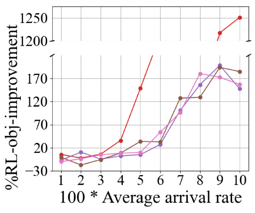
We compare the different policies in the following way. We run each of the heuristic policies on $100$ randomly generated streams each of $300s$ long, for each average arrival rate. For the learnt policies from CML approach, we run each of the $10$ trained policies on $10$ randomly generated streams (hence $100$ random streams), for each average arrival rate in the simulation (refer to Table II). We remove the data of first $90$s in each stream to neglect transient traffic behaviour and compute the average (over $100$ streams) of the control objective values (value of the objective function of Problem (5) with the first $T_{h}$ seconds of a robot’s trajectory data) from generated streams. We call this the average performance of policy $p$, denoted by $\bar{J}_{p}$, for a given arrival rate. We then compare the average performance of the learnt CML policy against some policy $p$ using the quantity

$$\text{\%RL-obj-improvment}_{p}:=\frac{\bar{J}_{CML}-\bar{J}_{p}}{\bar{J}_{p}}\%$$

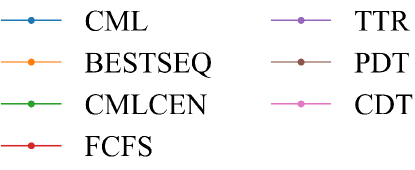
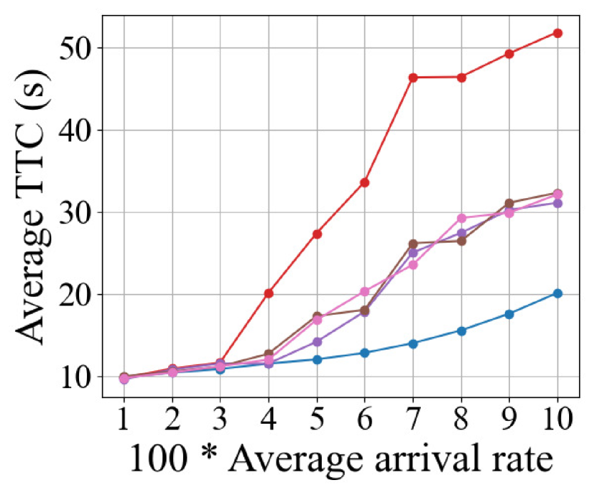
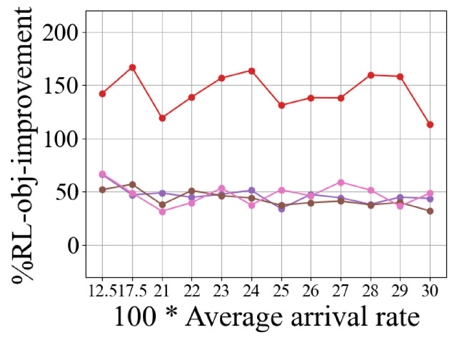
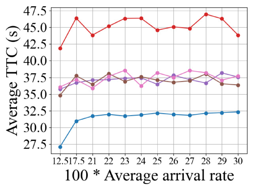
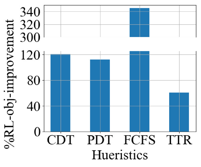
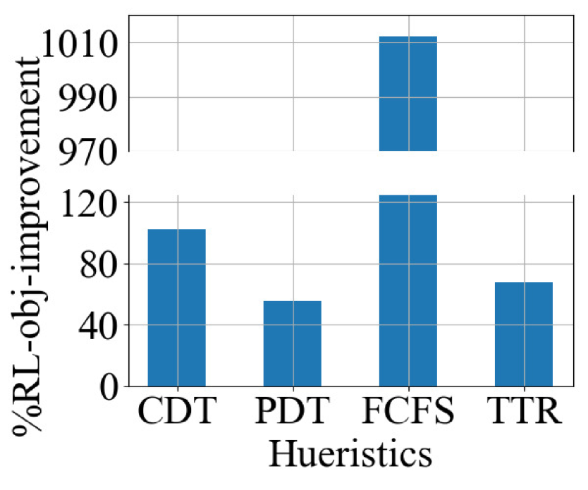
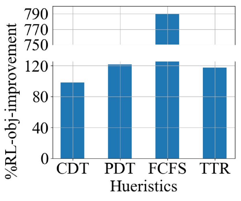
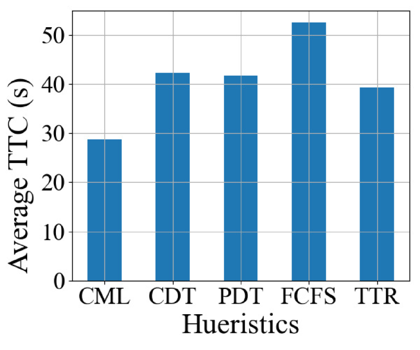
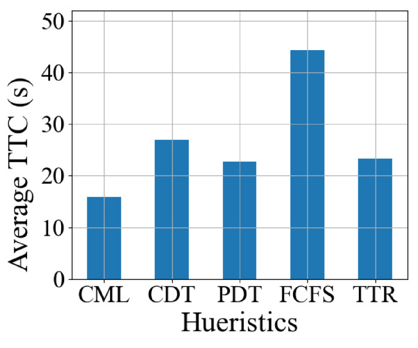
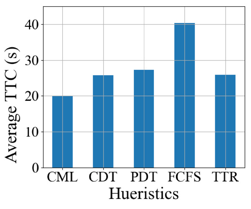
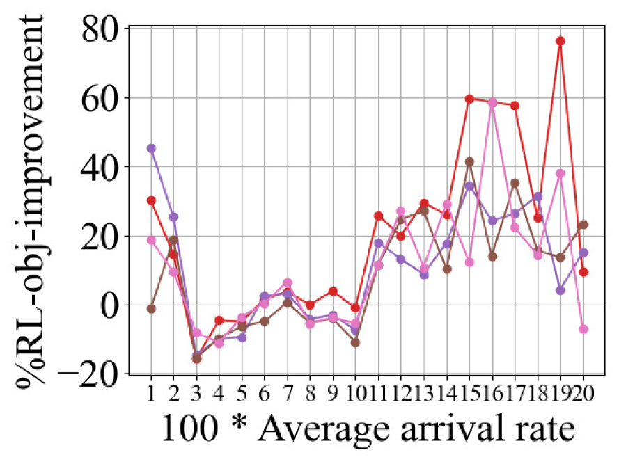
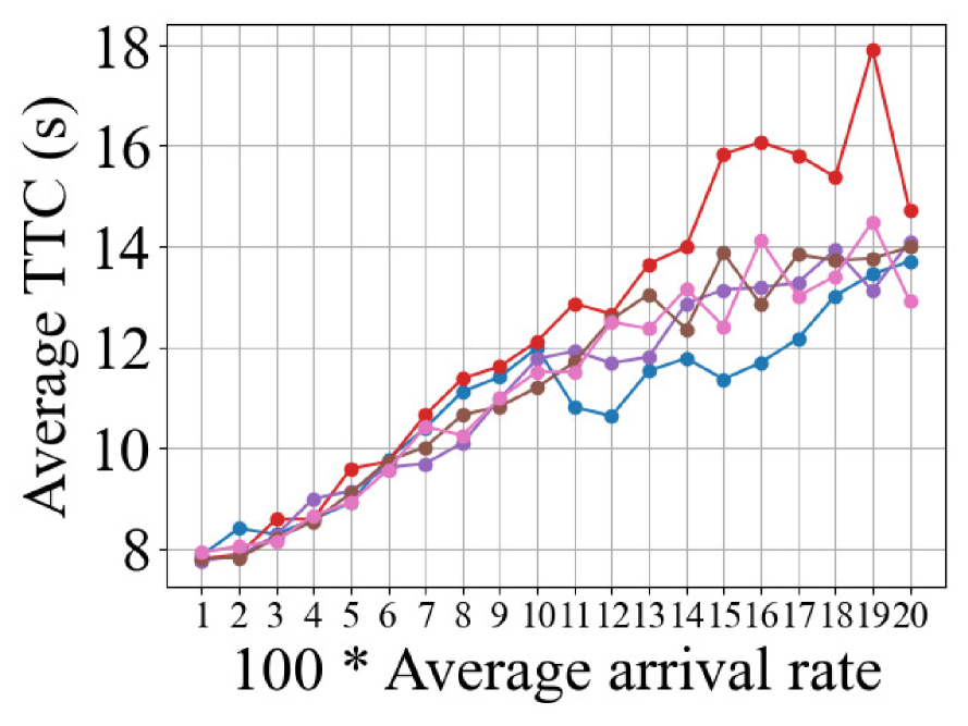
for each average arrival rate in the test cases. This quantity specifies how suboptimal the policy $p$ is compared to the learnt CML policy. We also compare the learnt policies against the heuristics using average (over all robots) time to cross (TTC) the intersection since their entry into RoI. Figures 4 through 8 compare the performance of different heuristics against the policies learnt using CML after $100000$ learning iterations under different traffic and parameter configurations. The common legend for Figures 4, 5 and  6 is in Figure 3.

Figure 3: Legend for Figures 4, 5 and  6.

Figures 4 and 5

(a)

(b)

(c)

(d)

Figure 4: Percentage improvement in average performance of CML trained policies over that of different policies (Figures (a), (b), (c) and (d) for Sim-1, Sim-2, Sim-3 and Sim-4 respectively). Dashed black line is $0\%$). See Figure 3 for legend.

(a)

(b)

(c)

(d)

Figure 5: Average time to cross (TTC) for different policies (Figures (a), (b), (c) and (d) for Sim-1, Sim-2, Sim-3 and Sim-4 respectively). See Figure 3 for legend.

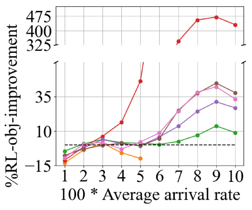
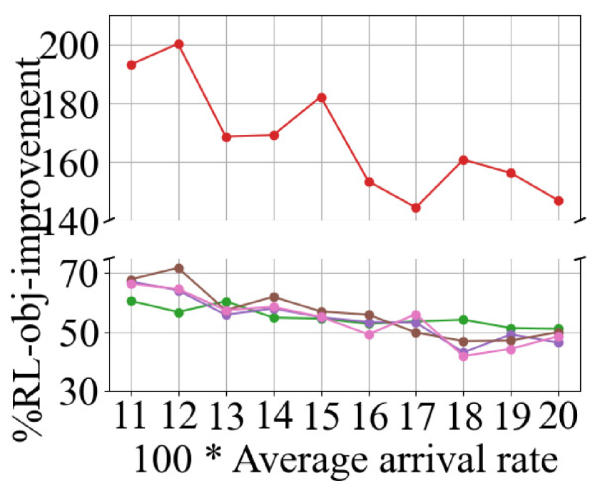
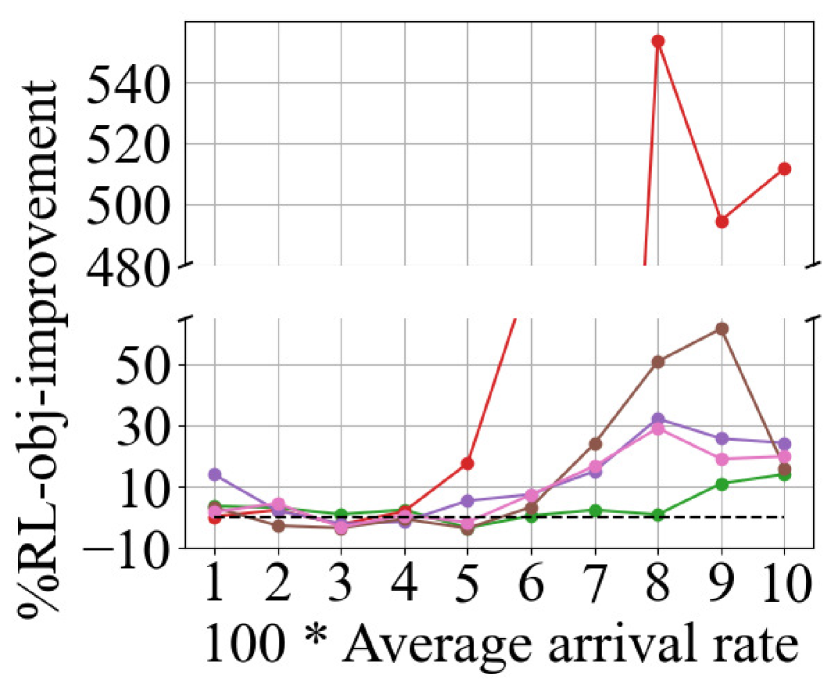
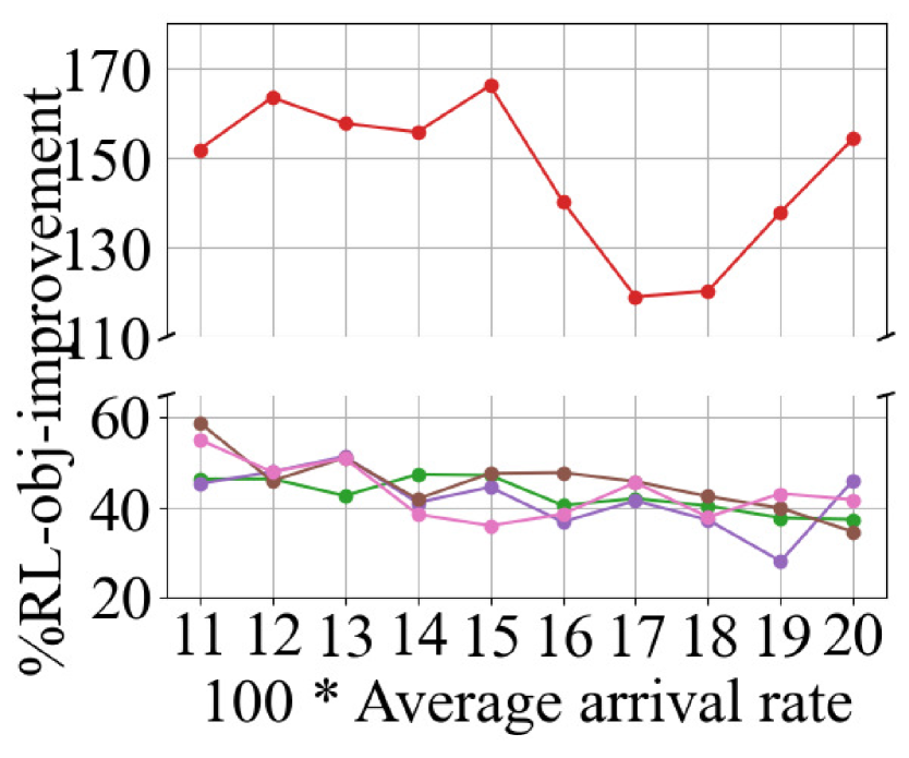
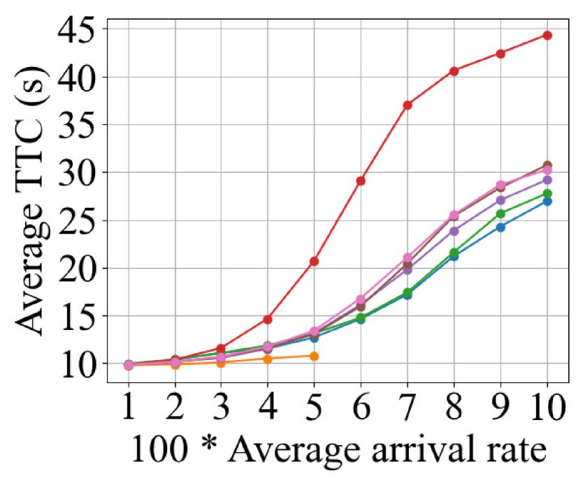
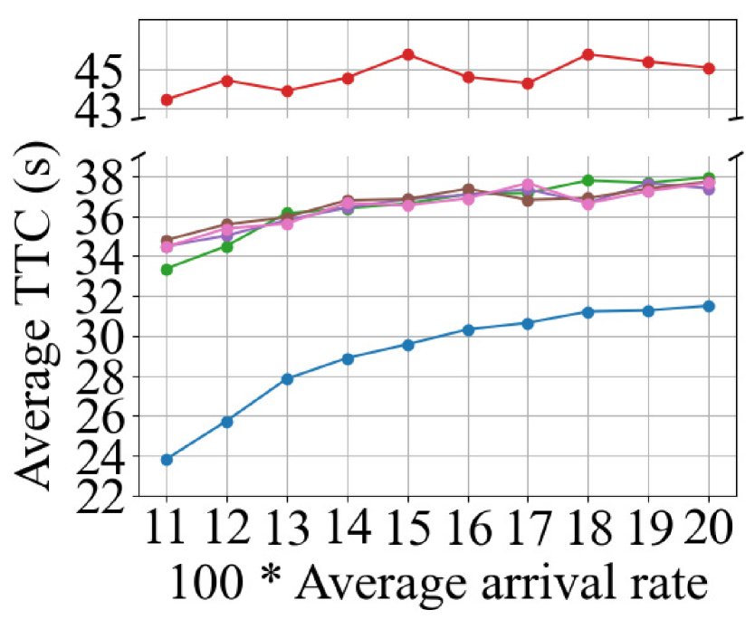
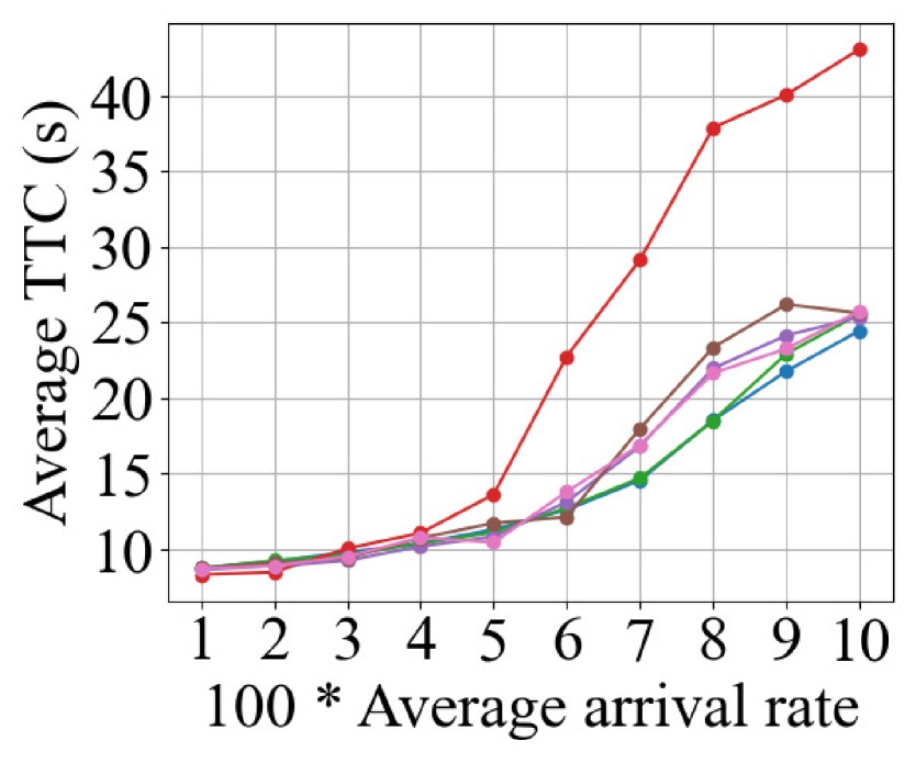
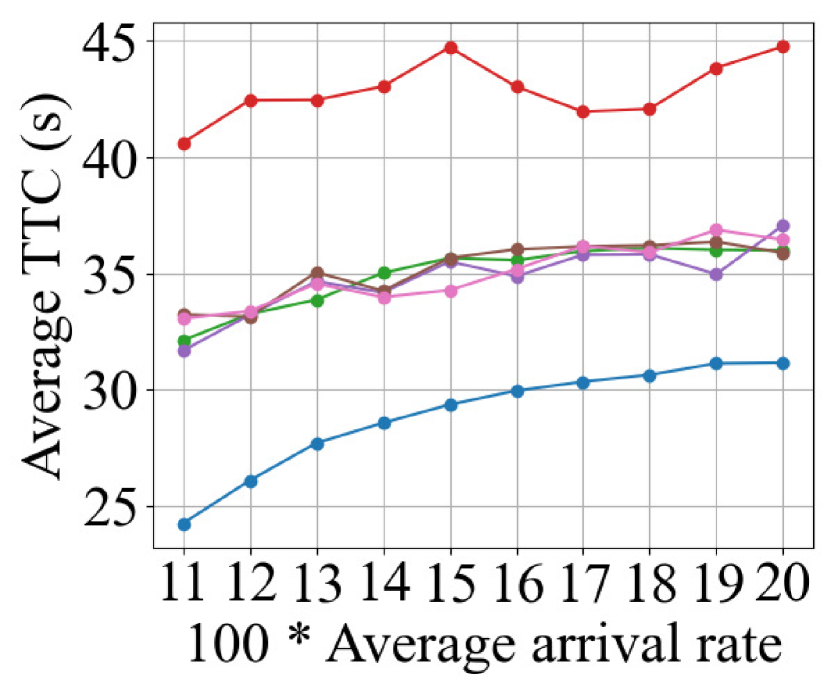
compare the performance of CML policies over other policies, in homogeneous traffic setting. We see that CML policy, in general, outperforms all the heuristics by a good margin both in terms of average performance and average TTC over a large range of average arrival rates. Note that average TTC is an inverse measure of average intersection throughput (low TTC implies high intersection throughput). We also note that the central CML (CMLCEN) policy performs poorly compared to the shared CML policy. This may be due to increase in the number of parameters to be learnt in a central policy and possibly more local minima which come along with it. Since BESTSEQ is computationally expensive, we present comparisons of CML and other heuristics against BESTSEQ only for the set-up in Sim-1 (Figures LABEL:fig:obj_gap_sim_1 and LABEL:fig:avg_ttc_sim_1), that too for arrival rates $0.01$ to $0.05$ robots/lane/s. Beyond this arrival rate, the computation time for BESTSEQ is prohibitively large. For very low arrival rates ($0.01$ to $0.04$ robots/lane/s), we notice that the heuristics do better than CML trained policies. This may be because a CML policy generalizes for better performance over a large range of average arrival rates.

In Figure 6 (results related to Sim-6 and Sim-7), we see that the policies trained on homogeneous traffic setting on a range of average arrival rates $\{0.11,0.12,...,0.2\}$ outperform other heuristics in test traffic generated using other average arrival rates too. Figures LABEL:fig:obj_gap_sim_5 and LABEL:fig:avg_ttc_sim_5 present comparisons between different policies in heterogeneous traffic setting (Sim-5). In Sim-5, the CML policy outperforms other heuristics by a large margin. We observe a larger gap in the average TTC compared to homogeneous traffic setting. This may be due to the bad performance of heuristics in such settings. We see similar results when the same trained policies are tested on time varying traffics – homogeneous burst-mode traffic (Sim-8) presented in Figures LABEL:fig:obj_gap_sim_8 and LABEL:fig:avg_ttc_sim_8 and heterogeneous random traffic (Sim-9) presented in Figures LABEL:fig:obj_gap_sim_9 and LABEL:fig:avg_ttc_sim_9. Figures 6, LABEL:fig:obj_gap_sim_8,  LABEL:fig:obj_gap_sim_9, LABEL:fig:avg_ttc_sim_8 and LABEL:fig:avg_ttc_sim_9 also demonstrate that the learnt CML policies generalize well to traffic situations unseen during training.

(a)

(b)

(c)

(d)

Figure 6: Percentage improvement in average performance of CML trained policies over that of different policies ((a) for Sim-6 and (c) for Sim-7). Average time to cross (TTC) for each policy ((b) for Sim-6 and (d) for Sim-7). See Figure 3 for legend.

(a)

(b)

(c)

Figure 7: Percentage improvement in average performance of CML trained policies over that of different policies (Figures (a), (b) and (c) for Sim-5, Sim-8 and Sim-9 respectively).

(a)

(b)

(c)

Figure 8: Average time to cross (TTC) for different policies (Figures (a), (b) and (c) for Sim-5, Sim-8 and Sim-9 respectively).

VI Implementation in a lab setting

We implemented the proposed algorithm on a collection of line following robots, specifically 3pi+ 32U4 Turtle edition robots manufactured by Pololu Robotics and Electronics [53]. Due to the lack of significant computational and communicational capabilities on these robots, we run the algorithm on a computer, store the computed trajectories and use XBee S6B WiFi modules to communicate the trajectories to the robots at each time-step. We use OptiTrack motion capture system [54] to track these robots. We use a 4-way intersection layout as in Figure 9 printed on a flex-sheet. The black lines represent the lanes for the robots. The robots follow the lines to cross the intersection and loop around on the perimeter square and re-enter the RoI on a randomly chosen lane. This process continues repeatedly so that we have a continual stream of robots.

Figure 9: A schematic of the layout used for implementation on robots. The black lines represent the paths for the robots to follow. The union of red and blue shaded regions is the RoI and the blue shaded region is the intersection. The robots flow in the direction of the arrows depicted along with lane numbers. $a=0.8$m and $c=0.53$m

VI-A Adaptations for implementation

For practical implementation of the algorithm, we need to address the issues arising from the simplifying assumptions on tracking errors, communication delays and computation times made during the formulation in Section II. In order to relax these assumptions, we let a low level PID based position controller on each robot track the given reference trajectory faithfully with bounded errors and by assuming that the per-robot communication delay and computation times are bounded. Suppose that the bound on position tracking errors is $b$ units, bound on communication delay is $\delta$ units, bounds on computation time per robot are $\Delta_{p}$ units and $\Delta_{c}$ units for provisional phase and coordinated phase respectively. These bounds were determined by tedious and repeated experimentation. The tracking errors are handled by considering $\hat{L}_{j}=L_{j}+2b$ as the length of robot $j\in V$ for all computations in the algorithm. Notice that this affects both rear-end and intersection safety constraints.

Computation time and communication delays are handled by pre-computing the trajectories. That is if a robot $i$ is about to enter the RoI at time $t_{i}^{\mathcal{A}}$, we estimate its velocity of entry and compute the provisional phase trajectories at time $t_{i}^{\mathcal{A}}-\Delta_{p}-\delta$. Similarly, we initiate the computations for $k^{th}$ coordinated phase at $kT_{c}-N_{p}\Delta_{c}-\delta$ for the robots in $V_{p}$ at that time, where $N_{p}$ is an appropriate upper bound on the number of robots in $V_{p}$.

If the communication delays are small enough, the errors due to such delays can be merged with tracking errors by adding the maximum possible distance a robot $i\in V$ can cover during the communication delay period which is $\bar{v}_{i}\delta$. In this case, trajectory pre-computation times may not involve the communication delay term $\delta$. Since the communication delays are small in our experiments, we follow this method.

Note that the policy is trained offline in an ideal scenario without these adaptations. These adaptations to the algorithm are made only during implementation.

VI-B Parameters for experiments

The approach length for each lane in the RoI, $d(l)=0.8$m (depicted as $a$ in Figure 9) $\forall l\in\{1,2,3,4\}$ and the width of the intersection in $0.53$m (depicted as $c$ in Figure 9). The length of each robot is $0.1$m. The bound on inherent tracking errors and tracking errors due to communication delay was measured to be, $b=0.075$m. To allow for better trajectory tracking performance, we set $\bar{v}_{i}=0.25$m/s $\forall i\in V$, even though the robots are capable of speeds up to $0.4$m/s. Given these bounds, we chose $\hat{L}_{j}=0.15$m for buffer to address communication delays and tracking errors. We set $T_{c}=3$s and $T_{h}=20$s. We measured $\Delta_{p}=0.1$s and $\Delta_{c}=0.2$s after repeated experiments.

VI-C Indicative results from experiments

We deployed a policy that was learnt offline in ideal simulations (without tracking errors, communication and computation delays and restricting parameters only to the RoI) using CML approach. We trained a set of $10$ policies each with different network parameter initialization on the set of average arrival rates $\{0.11,0.12,...,0.2\}$ robots/lane/s. We tested these $10$ learnt policies in ideal simulation environment and chose the policy with the highest sum of average objective function value over the average arrival rates in the set $\{0.01,0.02,...,0.2\}$ robots/lane/s, over $10$ test simulations for each average arrival rate and compare its performance against the heuristics. The plots indicating the results of these simulations is presented in Figures LABEL:fig:obj_gap_exp_sim and LABEL:fig:ttc_exp_sim. We observe that, for the parameters considered in the experiments, the CML policies start to outperform the other heuristics only after an average arrival rate of $0.1$ robots/lane/s.

(a)

(b)

(c)

Figure 10: Figure (a): Percentage improvement in average performance of CML trained policy over that of different policies and Figure (b): Average time to cross (TTC) for different policies. Both the plots are under ideal simulation environment for parameters used in experiments. See Figure 3 for legend. Figure (c): Box plot of TTC values for $3$ runs of $3$ different initial positions each for different policies. The box represent the range of values between $1^{\text{st}}$ and $3^{\text{rd}}$ quartile, whiskers represent range of values between $10^{\text{th}}$ and $90^{\text{th}}$ percentile and bold black line represents the mean of the TTC values for each policy.

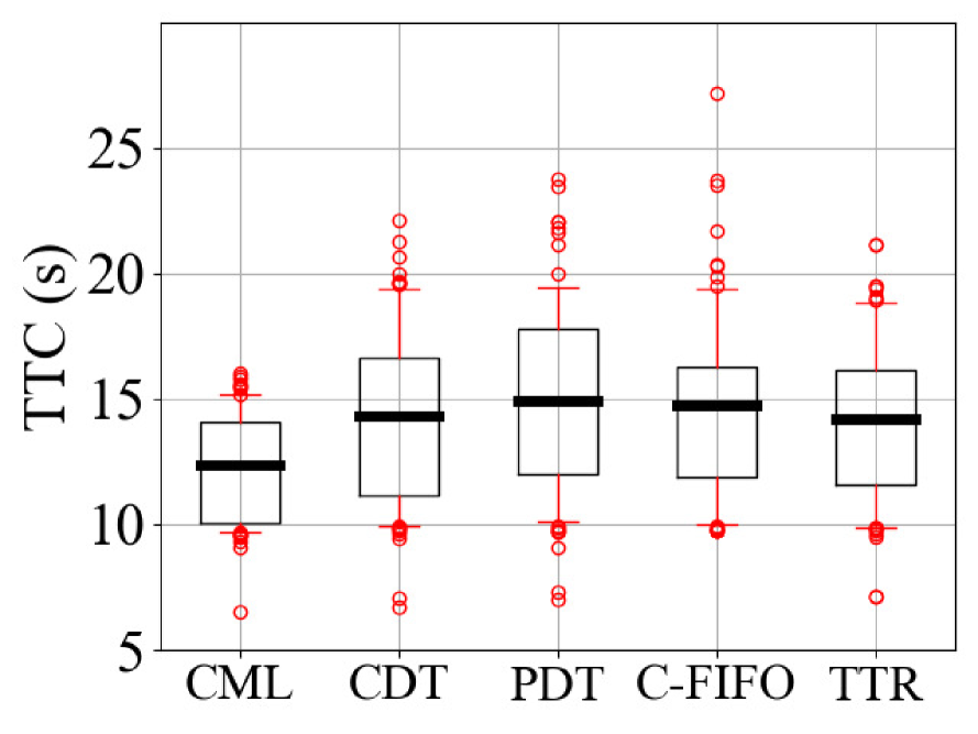
However, due to the limitations imposed in our lab setting (e.g., number of robots, approach length for each lane, velocity bounds on the robots etc.), it is hard to achieve such high average arrival rates consistently. For this reason, we choose to present some indicative experimental results for snapshots (sets $V_{p}$ and $V_{s}$).

In this regard, we consider the following $3$ different robot initializations on the outer ring (part of the path outside the RoI in Figure 9):

1. $2$ robots to enter each lane.

2. $3$ robots to enter two conflicting lanes and $1$ robot each to enter the other two lanes.

3. $2$ robots to enter two conflicting lanes, $3$ robots to enter one of the other and $1$ robot to enter the other.

The performance of the learnt policy is compared in the real-world set-up with the algorithmic adaptations proposed in the previous subsections against other heuristics by comparing the time to cross values such that each of the involved robots got through coordinated phase exactly once. The value of $T_{c}=5$s is chosen so that more robots participate in a coordinated phase. It is to be noted that the FCFS heuristic has an undue advantage in such a comparison since the trajectories are computed for a robot as and when it enters the RoI and does not have to wait till the next coordinated phase. Hence, to be fair for the heuristics, here we propose to compare with an alternate heuristic which we call C-FIFO, where the robots go through provisional phase and the crossing order (and hence the order in coordinated phase) follows the first-in first-out rule.

We conduct $3$ runs for each initialization for each policy (each run with same initial position of the robots) and present the average TTC obtained for different policies in Figure LABEL:fig:implmentation_results.

In Figure LABEL:fig:implmentation_results we observe that the CML policy produces low TTC values compared to other heuristics. We also observe that most of the TTC values for CML policy lie in a small region (e.g. range of values inside the box i.e., which fall within $1^{\text{st}}$ and $3^{\text{rd}}$ quartile) compared to other heuristics, thus promoting fairness in TTC among the involved robots in various scenarios. This is indicative of the performance of the CML policy deployed under real-time constraints.

VII Conclusions and future work

In this paper, we have combined learning with optimization methods to obtain a near-optimal solution for multi-robot unsignalized intersection management, which can be implemented in real-time. The proposed solution gives a policy that is shared by all the robots and can be deployed in a distributed manner. With extensive simulations, we have established that such a policy outperforms the major heuristics proposed in the literature, over a range of average traffic arrival rates. We also illustrate the vast improvement in computation time of the proposed solution compared to that of naive optimization methods for the intersection management problem. We have also proposed some adaptations to the solution framework to address real-world challenges like tracking errors, communication and computation delays and have implemented the learnt policies on robots in a lab setting with the proposed adaptations. Future works include implementation fine-tuning, extensions to allow lane changes, to handle disturbances, dynamic obstacles and for a network of intersections.

VIII Acknowledgements

We thank Ayush Das, Rithvik Mahajan and Soumyodipta Nath for their help in setting up and implementing the algorithm on robots in the lab setting. We also thank the Nokia Centre of Excellence in Networked Robotics at IISc for partially funding this project through the Nokia CSR grant.

Nishchal Hoysal G received his B.E. degree in Mechanical Engineering from BMS College of Engineering, Bengaluru, India in 2016. He is currently a Ph.D scholar in the Robert Bosch Center for Cyber Physical Systems at the Indian Institute of Science, Bengaluru, India. His research interests include learning methods for multi-agent planning and coordination.

Pavankumar Tallapragada (S’12-M’14) received the B.E. degree in Instrumentation Engineering from SGGS Institute of Engineering $\&$ Technology, Nanded, India in 2005, M.Sc. (Engg.) degree in Instrumentation from the Indian Institute of Science in 2007 and the Ph.D. degree in Mechanical Engineering from the University of Maryland, College Park in 2013. He was a Postdoctoral Scholar in the Department of Mechanical and Aerospace Engineering at the University of California, San Diego from 2014 to 2017. He is currently an Assistant Professor in the Department of Electrical Engineering and the Robert Bosch Centre for Cyber Physical Systems at the Indian Institute of Science. His research interests include networked control systems, distributed control, multi-agent systems and dynamics in social networks.

References

- [1] L. Chen and C. Englund, “Cooperative intersection management: A survey,” IEEE Transactions on Intelligent Transportation Systems, vol. 17, no. 2, pp. 570–586, 2015.
- [2] J. Rios-Torres and A. A. Malikopoulos, “A survey on the coordination of connected and automated vehicles at intersections and merging at highway on-ramps,” IEEE Transactions on Intelligent Transportation Systems, vol. 18, no. 5, pp. 1066–1077, 2016.
- [3] M. Khayatian, M. Mehrabian, E. Andert, R. Dedinsky, S. Choudhary, Y. Lou, and A. Shrivastava, “A survey on intersection management of connected autonomous vehicles,” ACM Transactions on Cyber-Physical Systems, vol. 4, no. 4, pp. 1–27, 2020.
- [4] S. A. Fayazi and A. Vahidi, “Mixed-integer linear programming for optimal scheduling of autonomous vehicle intersection crossing,” IEEE Transactions on Intelligent Vehicles, vol. 3, no. 3, pp. 287–299, 2018.
- [5] G. R. de Campos, P. Falcone, R. Hult, H. Wymeersch, and J. Sjöberg, “Traffic coordination at road intersections: Autonomous decision-making algorithms using model-based heuristics,” IEEE Intelligent Transportation Systems Magazine, vol. 9, no. 1, pp. 8–21, 2017.
- [6] S. A. Fayazi, A. Vahidi, and A. Luckow, “Optimal scheduling of autonomous vehicle arrivals at intelligent intersections via MILP,” in 2017 American Control Conference (ACC). IEEE, 2017, pp. 4920–4925.
- [7] R. Hult, M. Zanon, S. Gros, and P. Falcone, “Optimal coordination of automated vehicles at intersections: Theory and experiments,” IEEE Transactions on Control Systems Technology, vol. 27, no. 6, pp. 2510–2525, 2018.
- [8] X. Qian, J. Gregoire, A. De La Fortelle, and F. Moutarde, “Decentralized model predictive control for smooth coordination of automated vehicles at intersection,” in European Control Conference. IEEE, 2015, pp. 3452–3458.
- [9] J. Lee and B. Park, “Development and evaluation of a cooperative vehicle intersection control algorithm under the connected vehicles environment,” IEEE Transactions on Intelligent Transportation Systems, vol. 13, no. 1, pp. 81–90, 2012.
- [10] J. Lee, B. B. Park, K. Malakorn, and J. J. So, “Sustainability assessments of cooperative vehicle intersection control at an urban corridor,” Transportation Research Part C: Emerging Technologies, vol. 32, pp. 193–206, 2013.
- [11] A. A. Malikopoulos, C. G. Cassandras, and Y. J. Zhang, “A decentralized energy-optimal control framework for connected automated vehicles at signal-free intersections,” Automatica, vol. 93, pp. 244–256, 2018.
- [12] A. A. Malikopoulos, L. Beaver, and I. V. Chremos, “Optimal time trajectory and coordination for connected and automated vehicles,” Automatica, vol. 125, p. 109469, 2021.
- [13] D. Gadginmath and P. Tallapragada, “Data-guided distributed intersection management for connected and automated vehicles,” in 2022 American Control Conference (ACC), 2022, pp. 767–774.
- [14] K. Dresner and P. Stone, “A multiagent approach to autonomous intersection management,” Journal of Artificial Intelligence Research, vol. 31, pp. 591–656, March 2008.
- [15] M. Hausknecht, T. C. Au, and P. Stone, “Autonomous intersection management: Multi-intersection optimization,” in RSJ International Conference on Intelligent Robots and Systems, 2011, pp. 4581–4586.
- [16] P. Tallapragada and J. Cortés, “Hierarchical-distributed optimized coordination of intersection traffic,” IEEE Transactions on Intelligent Transportation Systems, vol. 21, no. 5, pp. 2100–2113, 2019.
- [17] S. D. Kumaravel, A. A. Malikopoulos, and R. Ayyagari, “Optimal coordination of platoons of connected and automated vehicles at signal-free intersections,” IEEE Transactions on Intelligent Vehicles, vol. 7, no. 2, pp. 186–197, 2022.
- [18] B. Chalaki and A. A. Malikopoulos, “A priority-aware replanning and resequencing framework for coordination of connected and automated vehicles,” IEEE Control Systems Letters, vol. 6, pp. 1772–1777, 2022.
- [19] M. Čáp, P. Novák, A. Kleiner, and M. Selecký, “Prioritized planning algorithms for trajectory coordination of multiple mobile robots,” IEEE Transactions on Automation Science and Engineering, vol. 12, no. 3, pp. 835–849, 2015.
- [20] G. R. de Campos, P. Falcone, and J. Sjöberg, “Autonomous cooperative driving: A velocity-based negotiation approach for intersection crossing,” in International IEEE Conference on Intelligent Transportation Systems. IEEE, 2013, pp. 1456–1461.
- [21] N. Suriyarachchi, F. M. Tariq, C. Mavridis, and J. S. Baras, “Real-time priority-based cooperative highway merging for heterogeneous autonomous traffic,” in IEEE International Intelligent Transportation Systems Conference (ITSC). IEEE, 2021, pp. 2019–2026.
- [22] H. Xu, W. Xiao, C. G. Cassandras, Y. Zhang, and L. Li, “A general framework for decentralized safe optimal control of connected and automated vehicles in multi-lane signal-free intersections,” IEEE Transactions on Intelligent Transportation Systems, vol. 23, no. 10, pp. 17 382–17 396, 2022.
- [23] S. Chamideh, W. Tärneberg, and M. Kihl, “A safe and robust autonomous intersection management system using a hierarchical control strategy and V2I communication,” IEEE Systems Journal, vol. 17, no. 1, pp. 50–61, 2023.
- [24] X. Pan, B. Chen, S. Timotheou, and S. A. Evangelou, “A convex optimal control framework for autonomous vehicle intersection crossing,” IEEE Transactions on Intelligent Transportation Systems, vol. 24, no. 1, pp. 163–177, 2023.
- [25] X. Pan, B. Chen, L. Dai, S. Timotheou, and S. A. Evangelou, “A hierarchical robust control strategy for decentralized signal-free intersection management,” IEEE Transactions on Control Systems Technology, pp. 1–16, 2023.
- [26] D. Carlino, S. D. Boyles, and P. Stone, “Auction-based autonomous intersection management,” in 16th International IEEE Conference on Intelligent Transportation Systems (ITSC). IEEE, 2013, pp. 529–534.
- [27] N. Suriyarachchi, R. Chandra, J. S. Baras, and D. Manocha, “GAMEOPT: Optimal real-time multi-agent planning and control for dynamic intersections,” in IEEE 25th International Conference on Intelligent Transportation Systems (ITSC), 2022, pp. 2599–2606.
- [28] C. Liu, C.-W. Lin, S. Shiraishi, and M. Tomizuka, “Distributed conflict resolution for connected autonomous vehicles,” IEEE Transactions on Intelligent Vehicles, vol. 3, no. 1, pp. 18–29, 2017.
- [29] C. Hubmann, M. Becker, D. Althoff, D. Lenz, and C. Stiller, “Decision making for autonomous driving considering interaction and uncertain prediction of surrounding vehicles,” in IEEE Intelligent Vehicles Symposium (IV). IEEE, 2017, pp. 1671–1678.
- [30] L. Zhao, S. Han, and Y. Lin, “Collision-aware multi-robot motion coordination deep-RL with dynamic priority strategy,” in IEEE 33rd International Conference on Tools with Artificial Intelligence (ICTAI). IEEE, 2021, pp. 65–72.
- [31] J. Cui, W. Macke, H. Yedidsion, A. Goyal, D. Urieli, and P. Stone, “Scalable multiagent driving policies for reducing traffic congestion,” in Proceedings of the 20th International Conference on Autonomous Agents and Multi Agent Systems, ser. AAMAS ’21, 2021, p. 386–394.
- [32] Y. Wu, H. Chen, and F. Zhu, “DCL-AIM: Decentralized coordination learning of autonomous intersection management for connected and automated vehicles,” Transportation Research Part C: Emerging Technologies, vol. 103, pp. 246–260, 2019.
- [33] T. Wu, M. Jiang, and L. Zhang, “Cooperative multiagent deep deterministic policy gradient (CoMADDPG) for intelligent connected transportation with unsignalized intersection,” Mathematical Problems in Engineering, vol. 2020, 2020.
- [34] U. Gunarathna, S. Karunasekera, R. Borovica-Gajic, and E. Tanin, “Real-time intelligent autonomous intersection management using reinforcement learning,” in 2022 IEEE Intelligent Vehicles Symposium (IV), 2022, pp. 135–144.
- [35] G.-P. Antonio and C. Maria-Dolores, “Multi-agent deep reinforcement learning to manage connected autonomous vehicles at tomorrow’s intersections,” IEEE Transactions on Vehicular Technology, vol. 71, no. 7, pp. 7033–7043, 2022.
- [36] B. Chalaki and A. A. Malikopoulos, “Robust learning-based trajectory planning for emerging mobility systems,” in American Control Conference (ACC), 2022, pp. 2154–2159.
- [37] M. Damani, Z. Luo, E. Wenzel, and G. Sartoretti, “PRIMAL2: Pathfinding via reinforcement and imitation multi-agent learning–lifelong,” IEEE Robotics and Automation Letters, vol. 6, no. 2, pp. 2666–2673, 2021.
- [38] J. S. Park, B. Tsang, H. Yedidsion, G. Warnell, D. Kyoung, and P. Stone, “Learning to improve multi-robot hallway navigation,” in Conference on Robot Learning. Proceedings of Machine Learning Research, 2021, pp. 1883–1895.
- [39] P. Long, T. Fan, X. Liao, W. Liu, H. Zhang, and J. Pan, “Towards optimally decentralized multi-robot collision avoidance via deep reinforcement learning,” in IEEE International Conference on Robotics and Automation (ICRA). IEEE, 2018, pp. 6252–6259.
- [40] Y. Yang and A. Whinston, “A survey on reinforcement learning for combinatorial optimization,” arXiv preprint arXiv:2008.12248, 2020.
- [41] I. Bello, H. Pham, Q. V. Le, M. Norouzi, and S. Bengio, “Neural combinatorial optimization with reinforcement learning,” arXiv preprint arXiv:1611.09940, 2016.
- [42] M. Nazari, A. Oroojlooy, L. Snyder, and M. Takác, “Reinforcement learning for solving the vehicle routing problem,” Advances in Neural Information Processing Systems, vol. 31, 2018.
- [43] D. Bertsimas and B. Stellato, “Online mixed-integer optimization in milliseconds,” INFORMS Journal on Computing, vol. 34, no. 4, pp. 2229–2248, 2022.
- [44] V. Digani, L. Sabattini, C. Secchi, and C. Fantuzzi, “Ensemble coordination approach in multi-AGV systems applied to industrial warehouses,” IEEE Transactions on Automation Science and Engineering, vol. 12, no. 3, pp. 922–934, 2015.
- [45] I. Draganjac, D. Miklić, Z. Kovačić, G. Vasiljević, and S. Bogdan, “Decentralized control of multi-AGV systems in autonomous warehousing applications,” IEEE Transactions on Automation Science and Engineering, vol. 13, no. 4, pp. 1433–1447, 2016.
- [46] X. Chen, Z. Xing, L. Feng, T. Zhang, W. Wu, and R. Hu, “An ETCEN-based motion coordination strategy avoiding active and passive deadlocks for multi-AGV system,” IEEE Transactions on Automation Science and Engineering, vol. 20, no. 2, pp. 1364–1377, 2023.
- [47] S. Dergachev and K. Yakovlev, “Distributed multi-agent navigation based on reciprocal collision avoidance and locally confined multi-agent path finding,” in 2021 IEEE 17th International Conference on Automation Science and Engineering (CASE), 2021, pp. 1489–1494.
- [48] F. Pratissoli, R. Brugioni, N. Battilani, and L. Sabattini, “Hierarchical traffic management of multi-AGV systems with deadlock prevention applied to industrial environments,” IEEE Transactions on Automation Science and Engineering, pp. 1–15, 2023.
- [49] J. van den Berg and M. Overmars, “Prioritized motion planning for multiple robots,” in 2005 IEEE/RSJ International Conference on Intelligent Robots and Systems, 2005, pp. 430–435.
- [50] P. Tallapragada and J. Cortés, “Distributed control of vehicle strings under finite-time and safety specifications,” IEEE Transactions on Control of Network Systems, vol. 5, no. 3, pp. 1399–1411, 2018.
- [51] X. Chu and H. Ye, “Parameter sharing deep deterministic policy gradient for cooperative multi-agent reinforcement learning,” arXiv preprint arXiv:1710.00336, 2017.
- [52] T. P. Lillicrap, J. J. Hunt, A. Pritzel, N. Heess, T. Erez, Y. Tassa, D. Silver, and D. Wierstra, “Continuous control with deep reinforcement learning,” arXiv preprint arXiv:1509.02971, 2015.
- [53] “3pi+ 32U4 Robot - Turtle Edition (75:1 LP Motors), Assembled,” https://www.pololu.com/product/3738, accessed: 2023-08-12.
- [54] “NaturalPoint, ”Motion Capture Systems-OptiTrack Webpage.”,” https://optitrack.com, accessed: 2023-08-12.
![[Uncaptioned image]](/html/2302.05082/assets/x26.png) |