11institutetext: B.V. Rathish Kumar* 22institutetext: Department of Mathematics and Statistics, Indian Institute of Technology, Kanpur, India
22email: drbvrk11@gmail.com*
33institutetext: Meena Pargaei 44institutetext: Department of Mathematics and Statistics, Indian Institute of Technology, Kanpur, India
Department of Mathematics, G.P.G.C. Champawat, Uttarakhand, India
44email: meenamenu15@gmail.com

An efficient Haar wavelet method for the coupled non-linear transient PDE-ODEs system with discontinuous coefficients

B.V. Rathish Kumar    Meena Pargaei
Abstract

In this work, Haar wavelet method for the coupled non-linear transient PDE-ODEs system with Neumann boundary condition has been proposed. The capability of the method in handling multiple jump discontinuities in the coefficients and parameters of the transient and coupled PDE-ODEs system is brought out through a series of 1D/2D/3D test problems. The method is easy to implement, computationally efficient and compare well with conventional methods like finite element method. Convergence analysis of the method has been carried out and apriori error is found to be exponential order i.e. uuHXo(2j)similar-tosubscriptnorm𝑢subscript𝑢𝐻𝑋𝑜superscript2𝑗\|u-u_{H}\|_{X}\sim o(2^{-j}). ILU-GMRES is found to better accelerate the numerical solution convergence than other Krylov solvers for the class of transient non-linear PDE-ODE system.

Keywords:
Non-linear coupled PDE-ODEs system Haar wavelet method Convergence analysis Jump discontinuity
journal: Journal of Scientific Computing

1 Introduction

Study of coupled PDE-ODEs systems has been an active research theme as such models arise in different fields of physical science, engineering, biology and economics. For instance such models are encountered while dealing with problems related to electro-magnetic coupling, coupling of chemical reaction and transport, mechanical coupling, propagation of electric waves in cardiac tissue etc. J. Doafouz et al. Daafouz et al. (2014) model for a boost converter connected to a load via a transmission line, coupled the partial differential equation describing telegraph with the ODE representing the action of the converter. In Göktepe and Kuhl (2010), E. Sabine presented the mathematical model of mitochondrial swelling phenomena via coupled PDE-ODE system. Such PDE-ODE coupled systems frequently arise in the field of cardiac electrophysiology Plonsey (1988); Keener and Sneyd (1998); Sepulveda et al. (1989). Such PDE-ODE coupled systems are not easily solvable especially when they are non-linear and in addition they have discontinuities or sharp variations either in field variables or coefficients or parameters appearing in the governing mathematical model. This is especially the case in mathematical models representing the cardiac electrical activity in ischemic cardiac tissue. Such discontinuities are also encountered in solid mechanics while dealing with fractures, cracks, inclusions and voids. In fluid mechanics such sharp variations in field variables arise when dealing with shock waves, boundary layers etc.

Several specialized numerical methods based on different operator discretization procedures such as finite differences, finite elements, spectral elements, finite volume etc. have been used to solve such coupled systems with discontinuities or sharp variations. M. Vynnycky and Sarah L. Mitchell Vynnycky and Mitchell (2013) proposed Keller box based finite difference method for parabolic PDE with discontinuous boundary conditions. Several finite element method based adaptive methods have been proposed to deal with jumps, kinks or sharp variations in PDE model. Andreas Bomto et al. in Bonito et al. (2013) proposed adaptive finite element method for elliptic problems with discontinuous coefficients for dealing with diffusion through porous media, or rough surfaces, electromagnetic field propagation on heterogeneous media using distortion theory. C. Bernardi and R. Verfurth in Bernardi and Verfürth (2000) derived apriori and aposteriori errors for adaptive finite element method for elliptic equations with non-smooth coefficients for modeling multilayer fluids with different viscosities. In Bonito and Devaud (2015), Andrea Bonito and Denis Devand introduced the adaptive finite element method for stokes problem with discontinuities viscosity. There are also meshfree approximation techniques which provide greater flexibility. C. Armando Duarte and J.T. Oden Duarte and Oden (1996) implemented h-p cloud method, fully exploiting the h, p and h-p adaptivity, devoid of conventional finite element grids on Poisson problems and 3-D elasticity problem. However these methods are not only limited by their adaptivity approach but may turn out to be very costly especially when dealing with the problems with evolving and moving features. In Fries and Belytschko (2010), generalized or extended finite element method has been discussed especially to effectively handle the jumps and singularities but this again gets quite sensitive to indicator function choice and are computationally costly.

Recently, wavelet methods are getting much attention, due to their inherent adaptability to the complexities such as discontinuities, sharp variations etc. in solving the mathematical models from science and engineering. Its properties such as orthogonality, compact support, arbitrary regularity and high order vanishing moments are very attractive. Wavelet based Galerkin and collocation methods have been used to solve integral equations, ODEs, PDEs, fractional differential equationsAziz et al. (2013a, 2010b); Šarler et al. (2011); Aziz et al. (2013b); Aziz and Fayyaz (2013); Aziz et al. (2010a, 2011, 2012); Comincioli et al. (2000); Wu (2009). In Paolucci et al. (2014) parallel wavelet adaptive method has been used in the domain decomposition framework to solve the compressible reacting flow with the shock wave in air. Oleg V. Vasilyev et al. Vasilyev et al. (2004) have developed discontinuous interpolating wavelets for handling multiphase problems with discontinuities across the phase boundaries. Kai Schneider and Oleg V. Vasiley Schneider and Vasilyev (2010) demonstrated the ability of adaptive wavelet basis in capturing coherent vortex structures in turbulent flows and thereby zoomed into their space-scale structure. They also present a hierarchy of wavelet-based turbulence models for carrying out complex industrial flow simulations. In Kestler et al. (2016) Sebastion Kestler et al. have introduced a space-time adaptive wavelet Galerkin method for time periodic PDEs. In all these studies authors have focused on using either Daubechies class of continuous wavelets or second generation wavelets. Simplest of all the wavelets and easy to implement in a finite domain is the Haar wavelet.

Haar wavelets are piecewise constant functions which are orthogonal and have compact support. They also have scaling property. The ease of using a Haar wavelet has made it very popular in signal processing and image processing. Because of the discontinuity of Haar wavelets, their derivatives does not exists and hence cannot be directly used in approximating solution of a differential equation. Chen and Hsiao Chen and Hsiao (1997) have proposed the idea that the highest order derivative of the differential equation can be expanded into the Haar series and not the field variable function. Then on integration one can obtain lower order derivatives and the function too.

Haar wavelet method has been used to solve the linear and non-linear differential equations and the eigenvalue problems Bujurke et al. (2008); Lepik (2007); Hariharan and Kannan (2010); Singh and Kumar (2017); Shi and Cao (2012). Largely these attempts are confined to 1D studies and this is specially the case with transient PDEs. Further no attempt has been made to test Haar wavelet capability in handling complexities like discontinuities, sharp variations etc. In this work, we propose the Haar wavelet method for the solution of coupled PDE-ODEs system with Neumann boundary condition and having discontinuities in either in source/coefficient function or in any parameter of the model. We will show the power of method in handling problem with multiple discontinuities like those which occur in cardiac electrophysiological models. We easily extend the method to higher dimensions and also to identify the desired linear solver and the influence of preconditioning in convergence acceleration. We also theoretically carry out the error analysis and show that the convergence is of exponential order i.e. o(2j)𝑜superscript2𝑗o(2^{-j}). We compare the results against those from finite element method both for quality and computational complexity. The paper is organized as follows:

In section 2, we introduce Haar wavelet function, its properties and haar integrating functions. In the next section, one and two dimensional Haar wavelet method for non-linear PDE-ODEs system will be developed. Convergence analysis of the proposed method is presented in section 4. Numerical results and discussion for the several problems with different types of discontinuities are provided in section 5. Three dimensional Haar wavelet method is discussed in the next section and its convergence analysis has been established. Further the proposed method has been successfully demonstrated for few practical problems, with discontinuity from cardiac electrophysiology in ischemic cardiac tissue.

2 Haar wavelets

Let us consider the interval x[A,B]𝑥𝐴𝐵x\in[A,B], A, B are finite real numbers. Define M=2J𝑀superscript2𝐽M=2^{J}, J𝐽J is the maximum level of resolution. This interval [A,B]𝐴𝐵[A,B] is equally divided into 2M2𝑀2M subintervals such that the length of each subinterval is Δx=(BA)/2MΔ𝑥𝐵𝐴2𝑀\Delta x=(B-A)/2M. Now, define the dilation and translation parameter j=0,1,,J𝑗01𝐽j=0,1,...,J and k=0,1,,m1𝑘01𝑚1k=0,1,...,m-1 respectively, where, m=2j𝑚superscript2𝑗m=2^{j}. The wavelet number is given by i=m+k+1𝑖𝑚𝑘1i=m+k+1. Family of haar wavelets is defined as follows:

For i=1𝑖1i=1

hi(x)={1when Ax<B0otherwise.subscript𝑖𝑥cases1when 𝐴𝑥𝐵0otherwise\displaystyle h_{i}(x)=\begin{cases}1&\text{when }A\leq\ x<B\\ 0&\text{otherwise}.\end{cases}

For i2𝑖2i\geq 2

hi(x)={1when β1(i)x<β2(i)1when β2(i)x<β3(i)0otherwise,subscript𝑖𝑥cases1when subscript𝛽1𝑖𝑥subscript𝛽2𝑖1when subscript𝛽2𝑖𝑥subscript𝛽3𝑖0otherwise\displaystyle h_{i}(x)=\begin{cases}1&\text{when }\beta_{1}(i)\leq\ x<\beta_{2}(i)\\ -1&\text{when }\beta_{2}(i)\leq\ x<\beta_{3}(i)\\ 0&\text{otherwise},\end{cases} (1)

where,

β1(i)=A+2kζΔx,β2(i)=A+(2k+1)ζΔx,formulae-sequencesubscript𝛽1𝑖𝐴2𝑘𝜁Δ𝑥subscript𝛽2𝑖𝐴2𝑘1𝜁Δ𝑥\displaystyle\beta_{1}(i)=A+2k\zeta\Delta x,\hskip 14.22636pt\beta_{2}(i)=A+(2k+1)\zeta\Delta x,
β3(i)=A+2(k+1)ζΔx,ζ=M/m.formulae-sequencesubscript𝛽3𝑖𝐴2𝑘1𝜁Δ𝑥𝜁𝑀𝑚\displaystyle\beta_{3}(i)=A+2(k+1)\zeta\Delta x,\hskip 14.22636pt\zeta=M/m.

Haar wavelets are orthogonal, since

ABhp(x)hq(x)𝑑x={2q(BA)when p=q0when pq.superscriptsubscript𝐴𝐵subscript𝑝𝑥subscript𝑞𝑥differential-d𝑥casessuperscript2𝑞𝐵𝐴when 𝑝𝑞0when 𝑝𝑞\displaystyle\int_{A}^{B}h_{p}(x)h_{q}(x)dx=\begin{cases}2^{-q}(B-A)&\text{when }p=q\\ 0&\text{when }p\neq q.\end{cases}

For the solution of differential equation, we have to compute the integral

pα,i(x)=∫⋯∫ABhi(t)𝑑tα=1(α1)!Ax(xt)(α1)hi(t)𝑑t,subscript𝑝𝛼𝑖𝑥superscriptsubscriptmultiple-integral𝐴𝐵subscript𝑖𝑡differential-dsuperscript𝑡𝛼1𝛼1superscriptsubscript𝐴𝑥superscript𝑥𝑡𝛼1subscript𝑖𝑡differential-d𝑡\displaystyle p_{\alpha,i}(x)=\idotsint_{A}^{B}h_{i}(t)dt^{\alpha}=\frac{1}{(\alpha-1)!}\int_{A}^{x}(x-t)^{(\alpha-1)}h_{i}(t)dt, (2)

where α=1,2,,n𝛼12𝑛\alpha=1,2,...,n and i=1,2,,2M𝑖122𝑀i=1,2,...,2M.

For the case, α=0,p0,i(x)=hi(x)formulae-sequence𝛼0subscript𝑝0𝑖𝑥subscript𝑖𝑥\alpha=0,p_{0,i}(x)=h_{i}(x).

This integral is calculated with the help of equation (1), defined as

pα,i(x)={0when x<β1(i)1α!(xβ1(i))αwhen β1(i)x<β2(i)1α![(xβ1(i))α2(xβ2(i))α]when β2(i)x<β2(i)1α![(xβ1(i))α2(xβ2(i))α+(xβ3(i))α)]when x>β3(i).\displaystyle p_{\alpha,i}(x)=\begin{cases}0&\text{when }x<\beta_{1}(i)\\ \frac{1}{\alpha!}(x-\beta_{1}(i))^{\alpha}&\text{when }\beta_{1}(i)\leq\ x<\beta_{2}(i)\\ \frac{1}{\alpha!}[(x-\beta_{1}(i))^{\alpha}-2(x-\beta_{2}(i))^{\alpha}]&\text{when }\beta_{2}(i)\leq\ x<\beta_{2}(i)\\ \frac{1}{\alpha!}[(x-\beta_{1}(i))^{\alpha}-2(x-\beta_{2}(i))^{\alpha}+(x-\beta_{3}(i))^{\alpha})]&\text{when }x>\beta_{3}(i).\end{cases} (3)

When α=1,2𝛼12\alpha=1,2,

p1,i(B)={(BA)when i=10otherwise.subscript𝑝1𝑖𝐵cases𝐵𝐴when 𝑖10otherwise\displaystyle p_{1,i}(B)=\begin{cases}(B-A)&\text{when }i=1\\ 0&\text{otherwise}.\end{cases} (4)
p2,i(B)={(BA)2/2when i=1(BA)2/4m2otherwise.subscript𝑝2𝑖𝐵casessuperscript𝐵𝐴22when 𝑖1superscript𝐵𝐴24superscript𝑚2otherwise\displaystyle p_{2,i}(B)=\begin{cases}(B-A)^{2}/2&\text{when }i=1\\ (B-A)^{2}/4m^{2}&\text{otherwise}.\end{cases}

For the grid points xk=A+kh,k=0,1,,2Mformulae-sequencesubscript𝑥𝑘𝐴𝑘𝑘012𝑀x_{k}=A+kh,k=0,1,...,2M, h=ΔxΔ𝑥h=\Delta x, collocation points are as follows:

yk=xk1+xk2,k=1,2,,2M.formulae-sequencesubscript𝑦𝑘subscript𝑥𝑘1subscript𝑥𝑘2𝑘122𝑀\displaystyle y_{k}=\frac{x_{k-1}+x_{k}}{2},k=1,2,...,2M. (5)

After this discretization, we define Haar matrix H𝐻H, and Haar Integral matrices P1,P2subscript𝑃1subscript𝑃2P_{1},P_{2} of size 2M×2M2𝑀2𝑀2M\times 2M as H(i,k)=hi(yk),P1(i,k)=p1,i(yk),P2(i,k)=p2,i(yk)formulae-sequence𝐻𝑖𝑘subscript𝑖subscript𝑦𝑘formulae-sequencesubscript𝑃1𝑖𝑘subscript𝑝1𝑖subscript𝑦𝑘subscript𝑃2𝑖𝑘subscript𝑝2𝑖subscript𝑦𝑘H(i,k)=h_{i}(y_{k}),P_{1}(i,k)=p_{1,i}(y_{k}),P_{2}(i,k)=p_{2,i}(y_{k}).

2.1 Function approximation

Any function f(x)L2[0,1)𝑓𝑥superscript𝐿201f(x)\in L^{2}[0,1) can be approximated in terms of the Haar wavelet series as

f(x)=i=1αihi(x),𝑓𝑥superscriptsubscript𝑖1subscript𝛼𝑖subscript𝑖𝑥\displaystyle f(x)=\sum_{i=1}^{\infty}\alpha_{i}h_{i}(x),

where the wavelet coefficients αisubscript𝛼𝑖\alpha_{i} are obtained by

αi=2j01f(x)hi(x)𝑑x.subscript𝛼𝑖superscript2𝑗superscriptsubscript01𝑓𝑥subscript𝑖𝑥differential-d𝑥\displaystyle\alpha_{i}=2^{j}\int_{0}^{1}f(x)h_{i}(x)dx.

Since only the finite number of terms are taken for the computational purpose therefore, the function approximation f𝑓f is given by

f(x)=i=12Mαihi(x).𝑓𝑥superscriptsubscript𝑖12𝑀subscript𝛼𝑖subscript𝑖𝑥\displaystyle f(x)=\sum_{i=1}^{2M}\alpha_{i}h_{i}(x).

where, M=2J𝑀superscript2𝐽M=2^{J}

2.2 Functions consisting the coefficient having jump discontinuities

Let us consider the domain [0,1]01[0,1] and a function f(x)𝑓𝑥f(x) defined on this domain given by

f(x)=k(x3+1.1x20.1x)𝑓𝑥𝑘superscript𝑥31.1superscript𝑥20.1𝑥\displaystyle f(x)=k(-x^{3}+1.1x^{2}-0.1x) (6)

where, k𝑘k is a parameter.

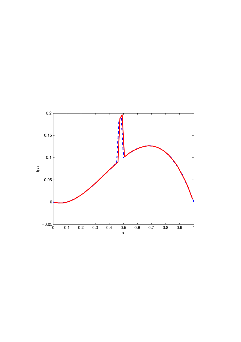
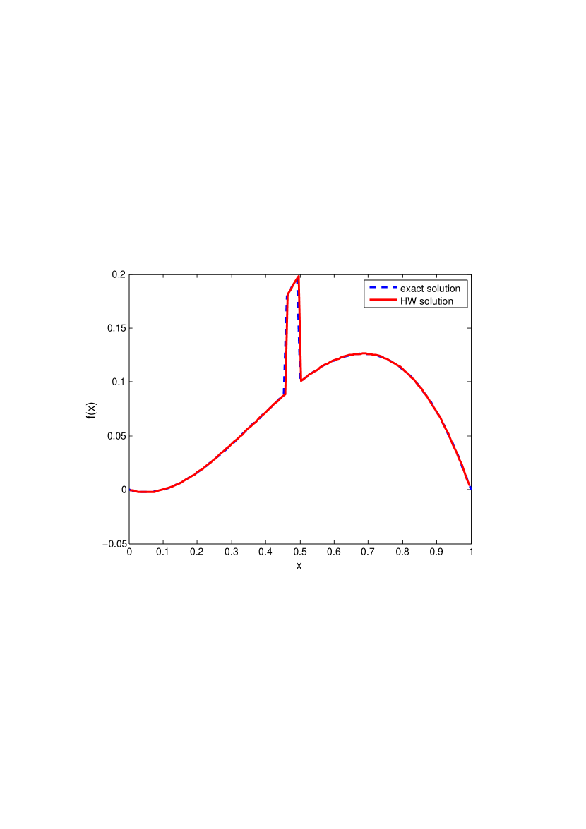
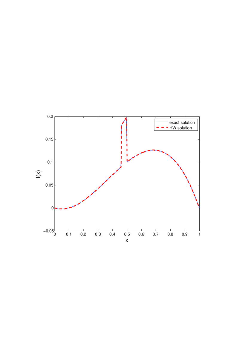
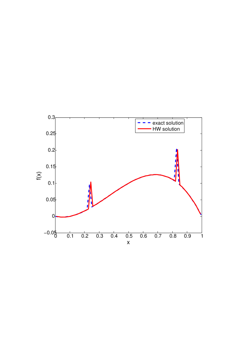
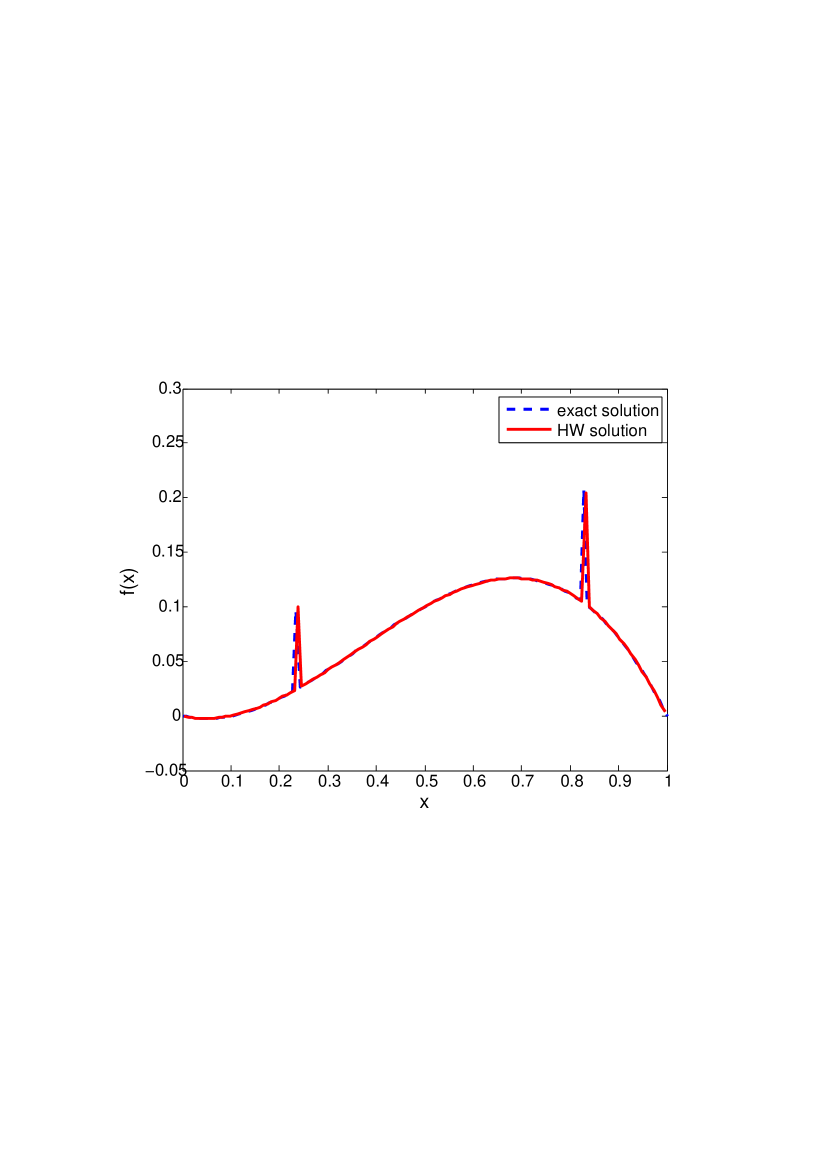
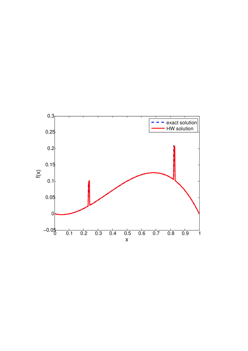
Now, if the parameter k𝑘k of the above function f(x)𝑓𝑥f(x) is discontinuities at one or multiple places of the domain, as given in Fig. 1(a) (k=1.5if0.46<x<0.5,k=1(k=1.5if0.46<x<0.5,k=1 otherwise) and Fig. 2(a) (k=4if0.2305<x<0.2383,k=2if0.8242<x<0.8302,k=1(k=4if0.2305<x<0.2383,k=2if0.8242<x<0.8302,k=1 otherwise), the corresponding function f(x)𝑓𝑥f(x) will also be discontinuous, drawn in Fig. 1(b) , 1(c), 1(d) 2(b), 2(c), and, 2(d) respectively.

Refer to caption
(a)
Refer to caption
(b)
Refer to caption
(c)
Refer to caption
(d)
Figure 1: (a) Value parameter k𝑘k, (b) Corresponding function f(x)𝑓𝑥f(x), J=5𝐽5J=5, (c) J=6𝐽6J=6, (d) J=7𝐽7J=7.
Refer to caption
(a)
Refer to caption
(b)
Refer to caption
(c)
Refer to caption
(d)
Figure 2: (a) Value parameter k𝑘k, (b) Corresponding function f(x)𝑓𝑥f(x) J=5𝐽5J=5 , (c) J=6𝐽6J=6, (d) J=7𝐽7J=7.

3 Mathematical Model

Let ΩRnΩsuperscript𝑅𝑛\Omega\subset R^{n} then a general non-linear parabolic reaction-diffusion equation coupled with the system of ODEs, is given as follows:

ϵvtdiv(D(x)v)+f(v,w)italic-ϵ𝑣𝑡𝑑𝑖𝑣𝐷𝑥𝑣𝑓𝑣𝑤\displaystyle\epsilon\frac{\partial v}{\partial t}-div(D(x)\nabla v)+f(v,w) =0absent0\displaystyle=0 xΩ,0tTformulae-sequence𝑥Ω0𝑡𝑇\displaystyle x\in\Omega,0\leq t\leq T
witgi(v,w)subscript𝑤𝑖𝑡subscript𝑔𝑖𝑣𝑤\displaystyle\frac{\partial w_{i}}{\partial t}-g_{i}(v,w) =0,absent0\displaystyle=0, xΩ,0tTformulae-sequence𝑥Ω0𝑡𝑇\displaystyle x\in\Omega,0\leq t\leq T
v(x,0)=v0(x,0),wi(x,0)𝑣𝑥0subscript𝑣0𝑥0subscript𝑤𝑖𝑥0\displaystyle v(x,0)=v_{0}(x,0),\hskip 14.22636ptw_{i}(x,0) =wi,0(x,0),absentsubscript𝑤𝑖0𝑥0\displaystyle=w_{i,0}(x,0), xΩ𝑥Ω\displaystyle x\in\Omega
nTD(x)vsuperscript𝑛𝑇𝐷𝑥𝑣\displaystyle n^{T}D(x)\nabla v =0,absent0\displaystyle=0, xΩ,0tT,formulae-sequence𝑥Ω0𝑡𝑇\displaystyle x\in\partial\Omega,0\leq t\leq T,

where, i=1,2,d𝑖12𝑑i=1,2,...d and D(x)𝐷𝑥D(x) is the diffusion tensor.

Remark: For existence-uniqueness and stability of such coupled system one may refer to Bourgault et al. (2006); Veneroni (2009).

3.1 Haar wavelet algorithm for the coupled non-linear PDE-ODEs system

Consider the three dimensional non-linear parabolic reaction-diffusion equation coupled with a system of ODEs given as follows:

ϵ(x,y,z)vtdiv(D(x,y,z)v)+f(v,w)=0,italic-ϵ𝑥𝑦𝑧𝑣𝑡𝑑𝑖𝑣𝐷𝑥𝑦𝑧𝑣𝑓𝑣𝑤0\displaystyle\epsilon(x,y,z)\frac{\partial v}{\partial t}-div(D(x,y,z)\nabla v)+f(v,w)=0, 0x,y,z1,0tTformulae-sequence0𝑥𝑦formulae-sequence𝑧10𝑡𝑇\displaystyle 0\leq x,y,z\leq 1,0\leq t\leq T (7)
wtg(v,w)=0,𝑤𝑡𝑔𝑣𝑤0\displaystyle\frac{\partial w}{\partial t}-g(v,w)=0, 0x,y,z1,0tTformulae-sequence0𝑥𝑦formulae-sequence𝑧10𝑡𝑇\displaystyle 0\leq x,y,z\leq 1,0\leq t\leq T (8)
v(x,y,z,0)=v0(x,y,z,0),w(x,y,z,0)=w0(x,y,z,0),formulae-sequence𝑣𝑥𝑦𝑧0subscript𝑣0𝑥𝑦𝑧0𝑤𝑥𝑦𝑧0subscript𝑤0𝑥𝑦𝑧0\displaystyle v(x,y,z,0)=v_{0}(x,y,z,0),\hskip 14.22636ptw(x,y,z,0)=w_{0}(x,y,z,0), 0x,y,z1formulae-sequence0𝑥𝑦𝑧1\displaystyle 0\leq x,y,z\leq 1 (9)

with Neumann boundary conditions in v𝑣v.

Let us write 7vtx2y2z2(x,y,z,t)superscript7𝑣𝑡superscript𝑥2superscript𝑦2superscript𝑧2𝑥𝑦𝑧𝑡\frac{\partial^{7}v}{\partial t\partial x^{2}\partial y^{2}\partial z^{2}}\big{(}x,y,z,t\big{)} in terms of the Haar wavelet as follows:

7vtx2y2z2(x,y,z,t)superscript7𝑣𝑡superscript𝑥2superscript𝑦2superscript𝑧2𝑥𝑦𝑧𝑡\displaystyle\frac{\partial^{7}v}{\partial t\partial x^{2}\partial y^{2}\partial z^{2}}(x,y,z,t) =i,j,k=12Mαi,jhi(x)hj(y)hk(z),t[ts,ts+1)formulae-sequenceabsentsuperscriptsubscript𝑖𝑗𝑘12𝑀subscript𝛼𝑖𝑗subscript𝑖𝑥subscript𝑗𝑦subscript𝑘𝑧𝑡subscript𝑡𝑠subscript𝑡𝑠1\displaystyle=\sum_{i,j,k=1}^{2M}\alpha_{i,j}h_{i}(x)h_{j}(y)h_{k}(z),\hskip 28.45274ptt\in[t_{s},t_{s+1}) (10)
wt(x,y,z,t)𝑤𝑡𝑥𝑦𝑧𝑡\displaystyle\frac{\partial w}{\partial t}(x,y,z,t) =l,m,n=12Mβl,m,nhl(x)hm(y)hn(z),t[ts,ts+1).formulae-sequenceabsentsuperscriptsubscript𝑙𝑚𝑛12𝑀subscript𝛽𝑙𝑚𝑛subscript𝑙𝑥subscript𝑚𝑦subscript𝑛𝑧𝑡subscript𝑡𝑠subscript𝑡𝑠1\displaystyle=\sum_{l,m,n=1}^{2*M}\beta_{l,m,n}h_{l}(x)h_{m}(y)h_{n}(z),\hskip 14.22636ptt\in[t_{s},t_{s+1}). (11)

Integrating equation (10) w.r.t t𝑡t from tssubscript𝑡𝑠t_{s} to t𝑡t, we will get

6vx2y2z2(x,y,z,t)superscript6𝑣superscript𝑥2superscript𝑦2superscript𝑧2𝑥𝑦𝑧𝑡\displaystyle\frac{\partial^{6}v}{\partial x^{2}\partial y^{2}\partial z^{2}}(x,y,z,t) =(tts)i,j,k=12Mαi,j,khi(x)hj(y)hk(z)+6vx2y2z2(x,y,z,ts),t[ts,ts+1).formulae-sequenceabsent𝑡subscript𝑡𝑠superscriptsubscript𝑖𝑗𝑘12𝑀subscript𝛼𝑖𝑗𝑘subscript𝑖𝑥subscript𝑗𝑦subscript𝑘𝑧superscript6𝑣superscript𝑥2superscript𝑦2superscript𝑧2𝑥𝑦𝑧subscript𝑡𝑠𝑡subscript𝑡𝑠subscript𝑡𝑠1\displaystyle=(t-t_{s})\sum_{i,j,k=1}^{2M}\alpha_{i,j,k}h_{i}(x)h_{j}(y)h_{k}(z)+\frac{\partial^{6}v}{\partial x^{2}\partial y^{2}\partial z^{2}}(x,y,z,t_{s}),\hskip 14.22636ptt\in[t_{s},t_{s+1}). (12)

Now, Integrate equation (12) twice w.r.t x𝑥x from 00 to x𝑥x also using the boundary conditions, we will obtain the following

4vy2z2(x,y,z,t)superscript4𝑣superscript𝑦2superscript𝑧2𝑥𝑦𝑧𝑡\displaystyle\frac{\partial^{4}v}{\partial y^{2}\partial z^{2}}(x,y,z,t) =(tts)i,j,k=12Mαi,j,kP2,i(x)hj(y)hk(z)+4vy2z2(x,y,z,ts)4vy2z2(0,y,z,ts)absent𝑡subscript𝑡𝑠superscriptsubscript𝑖𝑗𝑘12𝑀subscript𝛼𝑖𝑗𝑘subscript𝑃2𝑖𝑥subscript𝑗𝑦subscript𝑘𝑧superscript4𝑣superscript𝑦2superscript𝑧2𝑥𝑦𝑧subscript𝑡𝑠superscript4𝑣superscript𝑦2superscript𝑧20𝑦𝑧subscript𝑡𝑠\displaystyle=(t-t_{s})\sum_{i,j,k=1}^{2M}\alpha_{i,j,k}P_{2,i}(x)h_{j}(y)h_{k}(z)+\frac{\partial^{4}v}{\partial y^{2}\partial z^{2}}(x,y,z,t_{s})-\frac{\partial^{4}v}{\partial y^{2}\partial z^{2}}(0,y,z,t_{s})
+4vy2z2(0,y,z,t),t[ts,ts+1).superscript4𝑣superscript𝑦2superscript𝑧20𝑦𝑧𝑡𝑡subscript𝑡𝑠subscript𝑡𝑠1\displaystyle+\frac{\partial^{4}v}{\partial y^{2}\partial z^{2}}(0,y,z,t),\hskip 14.22636ptt\in[t_{s},t_{s+1}). (13)

Now, Integrate equation (3.1) twice w.r.t y𝑦y from 00 to y𝑦y also using the boundary conditions, we get

2vz2(x,y,z,t)superscript2𝑣superscript𝑧2𝑥𝑦𝑧𝑡\displaystyle\frac{\partial^{2}v}{\partial z^{2}}(x,y,z,t) =(tts)i,j,k=12Mαi,j,kP2,i(x)P2,j(y)hk(z)+2vz2(x,y,z,ts)2vz2(x,0,z,ts)2vz2(0,y,z,ts)absent𝑡subscript𝑡𝑠superscriptsubscript𝑖𝑗𝑘12𝑀subscript𝛼𝑖𝑗𝑘subscript𝑃2𝑖𝑥subscript𝑃2𝑗𝑦subscript𝑘𝑧superscript2𝑣superscript𝑧2𝑥𝑦𝑧subscript𝑡𝑠superscript2𝑣superscript𝑧2𝑥0𝑧subscript𝑡𝑠superscript2𝑣superscript𝑧20𝑦𝑧subscript𝑡𝑠\displaystyle=(t-t_{s})\sum_{i,j,k=1}^{2M}\alpha_{i,j,k}P_{2,i}(x)P_{2,j}(y)h_{k}(z)+\frac{\partial^{2}v}{\partial z^{2}}(x,y,z,t_{s})-\frac{\partial^{2}v}{\partial z^{2}}(x,0,z,t_{s})-\frac{\partial^{2}v}{\partial z^{2}}(0,y,z,t_{s})
+2vz2(0,0,z,ts)+2vz2(0,y,z,t)2vz2(0,0,z,t)+2vz2(x,0,z,t),t[ts,ts+1).superscript2𝑣superscript𝑧200𝑧subscript𝑡𝑠superscript2𝑣superscript𝑧20𝑦𝑧𝑡superscript2𝑣superscript𝑧200𝑧𝑡superscript2𝑣superscript𝑧2𝑥0𝑧𝑡𝑡subscript𝑡𝑠subscript𝑡𝑠1\displaystyle+\frac{\partial^{2}v}{\partial z^{2}}(0,0,z,t_{s})+\frac{\partial^{2}v}{\partial z^{2}}(0,y,z,t)-\frac{\partial^{2}v}{\partial z^{2}}(0,0,z,t)+\frac{\partial^{2}v}{\partial z^{2}}(x,0,z,t),\hskip 14.22636ptt\in[t_{s},t_{s+1}). (14)

Similarly, Integrate equation (3.1) twice w.r.t z𝑧z from 00 to z𝑧z also using the boundary conditions, we get

2vy2(x,y,z,t)superscript2𝑣superscript𝑦2𝑥𝑦𝑧𝑡\displaystyle\frac{\partial^{2}v}{\partial y^{2}}(x,y,z,t) =(tts)i,j,k=12Mαi,j,kP2,i(x)hj(y)P2,k(z)+2vy2(x,y,z,ts)2vy2(x,y,0,ts)2vy2(0,y,z,ts)absent𝑡subscript𝑡𝑠superscriptsubscript𝑖𝑗𝑘12𝑀subscript𝛼𝑖𝑗𝑘subscript𝑃2𝑖𝑥subscript𝑗𝑦subscript𝑃2𝑘𝑧superscript2𝑣superscript𝑦2𝑥𝑦𝑧subscript𝑡𝑠superscript2𝑣superscript𝑦2𝑥𝑦0subscript𝑡𝑠superscript2𝑣superscript𝑦20𝑦𝑧subscript𝑡𝑠\displaystyle=(t-t_{s})\sum_{i,j,k=1}^{2M}\alpha_{i,j,k}P_{2,i}(x)h_{j}(y)P_{2,k}(z)+\frac{\partial^{2}v}{\partial y^{2}}(x,y,z,t_{s})-\frac{\partial^{2}v}{\partial y^{2}}(x,y,0,t_{s})-\frac{\partial^{2}v}{\partial y^{2}}(0,y,z,t_{s})
+2vy2(0,y,0,ts)+2vy2(0,y,z,t)2vy2(0,y,0,t)+2vy2(x,y,0,t),t[ts,ts+1).superscript2𝑣superscript𝑦20𝑦0subscript𝑡𝑠superscript2𝑣superscript𝑦20𝑦𝑧𝑡superscript2𝑣superscript𝑦20𝑦0𝑡superscript2𝑣superscript𝑦2𝑥𝑦0𝑡𝑡subscript𝑡𝑠subscript𝑡𝑠1\displaystyle+\frac{\partial^{2}v}{\partial y^{2}}(0,y,0,t_{s})+\frac{\partial^{2}v}{\partial y^{2}}(0,y,z,t)-\frac{\partial^{2}v}{\partial y^{2}}(0,y,0,t)+\frac{\partial^{2}v}{\partial y^{2}}(x,y,0,t),\hskip 14.22636ptt\in[t_{s},t_{s+1}). (15)

Again, Integrating (12) twice w.r.t z𝑧z from 00 to z𝑧z and then twice w.r.t y𝑦y from 00 to y𝑦y also using the boundary conditions, we get

2vx2(x,y,z,t)superscript2𝑣superscript𝑥2𝑥𝑦𝑧𝑡\displaystyle\frac{\partial^{2}v}{\partial x^{2}}(x,y,z,t) =(tts)i,j,k=12Mαi,j,khi(x)P2,j(y)P2,k(z)+2vx2(x,y,z,ts)2vx2(x,0,z,ts)2vx2(x,y,0,ts)absent𝑡subscript𝑡𝑠superscriptsubscript𝑖𝑗𝑘12𝑀subscript𝛼𝑖𝑗𝑘subscript𝑖𝑥subscript𝑃2𝑗𝑦subscript𝑃2𝑘𝑧superscript2𝑣superscript𝑥2𝑥𝑦𝑧subscript𝑡𝑠superscript2𝑣superscript𝑥2𝑥0𝑧subscript𝑡𝑠superscript2𝑣superscript𝑥2𝑥𝑦0subscript𝑡𝑠\displaystyle=(t-t_{s})\sum_{i,j,k=1}^{2M}\alpha_{i,j,k}h_{i}(x)P_{2,j}(y)P_{2,k}(z)+\frac{\partial^{2}v}{\partial x^{2}}(x,y,z,t_{s})-\frac{\partial^{2}v}{\partial x^{2}}(x,0,z,t_{s})-\frac{\partial^{2}v}{\partial x^{2}}(x,y,0,t_{s})
+2vx2(x,0,0,ts)+2vx2(x,0,z,t)2vx2(x,0,0,t)+2vx2(x,y,0,t),t[ts,ts+1).superscript2𝑣superscript𝑥2𝑥00subscript𝑡𝑠superscript2𝑣superscript𝑥2𝑥0𝑧𝑡superscript2𝑣superscript𝑥2𝑥00𝑡superscript2𝑣superscript𝑥2𝑥𝑦0𝑡𝑡subscript𝑡𝑠subscript𝑡𝑠1\displaystyle+\frac{\partial^{2}v}{\partial x^{2}}(x,0,0,t_{s})+\frac{\partial^{2}v}{\partial x^{2}}(x,0,z,t)-\frac{\partial^{2}v}{\partial x^{2}}(x,0,0,t)+\frac{\partial^{2}v}{\partial x^{2}}(x,y,0,t),\hskip 14.22636ptt\in[t_{s},t_{s+1}). (16)

Now, Integrate equation (10) twice w.r.t. x , y and then z also using boundary conditions, we will obtain

vt(x,y,z,t)𝑣𝑡𝑥𝑦𝑧𝑡\displaystyle\frac{\partial v}{\partial t}(x,y,z,t) =i,j,k=12Mαi,j,kP2,i(x)P2,j(y)P2,k(z)+vt(0,y,z,t)vt(0,y,0,t)vt(0,0,z,t)+vt(0,0,0,t)absentsuperscriptsubscript𝑖𝑗𝑘12𝑀subscript𝛼𝑖𝑗𝑘subscript𝑃2𝑖𝑥subscript𝑃2𝑗𝑦subscript𝑃2𝑘𝑧𝑣𝑡0𝑦𝑧𝑡𝑣𝑡0𝑦0𝑡𝑣𝑡00𝑧𝑡𝑣𝑡000𝑡\displaystyle=\sum_{i,j,k=1}^{2M}\alpha_{i,j,k}P_{2,i}(x)P_{2,j}(y)P_{2,k}(z)+\frac{\partial v}{\partial t}(0,y,z,t)-\frac{\partial v}{\partial t}(0,y,0,t)-\frac{\partial v}{\partial t}(0,0,z,t)+\frac{\partial v}{\partial t}(0,0,0,t)
+vt(x,0,z,t)vt(x,0,0,t)+vt(x,y,0,t),t[ts,ts+1).𝑣𝑡𝑥0𝑧𝑡𝑣𝑡𝑥00𝑡𝑣𝑡𝑥𝑦0𝑡𝑡subscript𝑡𝑠subscript𝑡𝑠1\displaystyle+\frac{\partial v}{\partial t}(x,0,z,t)-\frac{\partial v}{\partial t}(x,0,0,t)+\frac{\partial v}{\partial t}(x,y,0,t),\hskip 14.22636ptt\in[t_{s},t_{s+1}). (17)

Now, Integrating the above equation (3.1) w.r.t. t𝑡t from tssubscript𝑡𝑠t_{s} to t𝑡t, we will get

v(x,y,z,t)𝑣𝑥𝑦𝑧𝑡\displaystyle v(x,y,z,t) =(tts)i,j,k=12Mαi,j,kP2,i(x)P2,j(y)P2,k(z)+v(x,y,z,ts)+v(0,y,z,t)v(0,y,z,ts)v(0,y,0,t)absent𝑡subscript𝑡𝑠superscriptsubscript𝑖𝑗𝑘12𝑀subscript𝛼𝑖𝑗𝑘subscript𝑃2𝑖𝑥subscript𝑃2𝑗𝑦subscript𝑃2𝑘𝑧𝑣𝑥𝑦𝑧subscript𝑡𝑠𝑣0𝑦𝑧𝑡𝑣0𝑦𝑧subscript𝑡𝑠𝑣0𝑦0𝑡\displaystyle=(t-t_{s})\sum_{i,j,k=1}^{2M}\alpha_{i,j,k}P_{2,i}(x)P_{2,j}(y)P_{2,k}(z)+v(x,y,z,t_{s})+v(0,y,z,t)-v(0,y,z,t_{s})-v(0,y,0,t)
+v(0,y,0,ts)v(0,0,z,t)+v(0,0,z,ts)+v(0,0,0,t)v(0,0,0,ts)+v(x,0,z,t)v(x,0,z,ts)𝑣0𝑦0subscript𝑡𝑠𝑣00𝑧𝑡𝑣00𝑧subscript𝑡𝑠𝑣000𝑡𝑣000subscript𝑡𝑠𝑣𝑥0𝑧𝑡𝑣𝑥0𝑧subscript𝑡𝑠\displaystyle+v(0,y,0,t_{s})-v(0,0,z,t)+v(0,0,z,t_{s})+v(0,0,0,t)-v(0,0,0,t_{s})+v(x,0,z,t)-v(x,0,z,t_{s})
v(x,0,0,t)+v(x,0,0,ts)+v(x,y,0,t)v(x,y,0,ts).𝑣𝑥00𝑡𝑣𝑥00subscript𝑡𝑠𝑣𝑥𝑦0𝑡𝑣𝑥𝑦0subscript𝑡𝑠\displaystyle-v(x,0,0,t)+v(x,0,0,t_{s})+v(x,y,0,t)-v(x,y,0,t_{s}). (18)

Again, Integrate (11) w.r.t t𝑡t from tssubscript𝑡𝑠t_{s} to t𝑡t, we acquire

w(x,y,z,t)=(tts)l,m,n=12Mβl,m,nhl(x)hm(y)hn(z)+w(x,y,z,ts)𝑤𝑥𝑦𝑧𝑡𝑡subscript𝑡𝑠superscriptsubscript𝑙𝑚𝑛12𝑀subscript𝛽𝑙𝑚𝑛subscript𝑙𝑥subscript𝑚𝑦subscript𝑛𝑧𝑤𝑥𝑦𝑧subscript𝑡𝑠\displaystyle w(x,y,z,t)=(t-t_{s})\sum_{l,m,n=1}^{2M}\beta_{l,m,n}h_{l}(x)h_{m}(y)h_{n}(z)+w(x,y,z,t_{s}) (19)

To find the solution at the collocation points, we have to discretized the equation (7) and (8) when tts+1𝑡subscript𝑡𝑠1t\rightarrow t_{s+1}.

The discrete form is as follows:

ϵ(xk1,yk2,zk3)vt(xk1,yk2,zk3,ts+1)[σl(xk1,yk2,zk3)2vx2(xk1,yk2,zk3,ts+1)+σl,x(xk1,yk2,zk3)vx(xk1,yk2,zk3,ts+1)\displaystyle\epsilon(x_{k_{1}},y_{k_{2}},z_{k_{3}})\frac{\partial v}{\partial t}(x_{k_{1}},y_{k_{2}},z_{k_{3}},t_{s+1})-\bigg{[}\sigma_{l}(x_{k_{1}},y_{k_{2}},z_{k_{3}})\frac{\partial^{2}v}{\partial x^{2}}(x_{k_{1}},y_{k_{2}},z_{k_{3}},t_{s+1})+\sigma_{l,x}(x_{k_{1}},y_{k_{2}},z_{k_{3}})\frac{\partial v}{\partial x}(x_{k_{1}},y_{k_{2}},z_{k_{3}},t_{s+1})
+(σt(xk1,yk2,zk3)2vy2(xk1,yk2,zk3,ts+1)+σt,y(xk1,yk2,zk3)vy(xk1,yk2,zk3,ts+1)+σt(xk1,yk2,zk3)\displaystyle+(\sigma_{t}(x_{k_{1}},y_{k_{2}},z_{k_{3}})\frac{\partial^{2}v}{\partial y^{2}}(x_{k_{1}},y_{k_{2}},z_{k_{3}},t_{s+1})+\sigma_{t,y}(x_{k_{1}},y_{k_{2}},z_{k_{3}})\frac{\partial v}{\partial y}(x_{k_{1}},y_{k_{2}},z_{k_{3}},t_{s+1})+\sigma_{t}(x_{k_{1}},y_{k_{2}},z_{k_{3}})
2vz2(xk1,yk2,zk3,ts+1)+σt,z(xk1,yk2,zk3)vz(xk1,yk2,zk3,ts+1)]+f(v(xk1,yk2,zk3,ts+1),w(xk1,yk2,zk3,\displaystyle\frac{\partial^{2}v}{\partial z^{2}}(x_{k_{1}},y_{k_{2}},z_{k_{3}},t_{s+1})+\sigma_{t,z}(x_{k_{1}},y_{k_{2}},z_{k_{3}})\frac{\partial v}{\partial z}(x_{k_{1}},y_{k_{2}},z_{k_{3}},t_{s+1})\bigg{]}+f(v(x_{k_{1}},y_{k_{2}},z_{k_{3}},t_{s+1}),w(x_{k_{1}},y_{k_{2}},z_{k_{3}},
ts+1))=0,\displaystyle t_{s+1}))=0, (20)
wt(xk1,yk2,zk3,ts+1)=g(v(xk1,yk2,zk3,ts+1),w(xk1,yk2,zk3,ts+1).\displaystyle\frac{\partial w}{\partial t}(x_{k_{1}},y_{k_{2}},z_{k_{3}},t_{s+1})=g(v(x_{k_{1}},y_{k_{2}},z_{k_{3}},t_{s+1}),w(x_{k_{1}},y_{k_{2}},z_{k_{3}},t_{s+1}). (21)

Using (11) at the grid points in (21) and linearize the non-linear terms by treating it explicitly, we obtain the following

l,m,n=12Mβl,m,nhl(xk1)hm(yk2)hn(zk3)=g(v(xk1,yk2,zk3,ts),w(xk1,yk2,zk3,ts)).superscriptsubscript𝑙𝑚𝑛12𝑀subscript𝛽𝑙𝑚𝑛subscript𝑙subscript𝑥subscript𝑘1subscript𝑚subscript𝑦subscript𝑘2subscript𝑛subscript𝑧subscript𝑘3𝑔𝑣subscript𝑥subscript𝑘1subscript𝑦subscript𝑘2subscript𝑧subscript𝑘3subscript𝑡𝑠𝑤subscript𝑥subscript𝑘1subscript𝑦subscript𝑘2subscript𝑧subscript𝑘3subscript𝑡𝑠\displaystyle\sum_{l,m,n=1}^{2M}\beta_{l,m,n}h_{l}(x_{k_{1}})h_{m}(y_{k_{2}})h_{n}(z_{k_{3}})=g(v(x_{k_{1}},y_{k_{2}},z_{k_{3}},t_{s}),w(x_{k_{1}},y_{k_{2}},z_{k_{3}},t_{s})).

Matrix system of the above equation is given by,

HlHmHnβ=c,subscript𝐻𝑙subscript𝐻𝑚subscript𝐻𝑛𝛽𝑐\displaystyle H_{l}H_{m}H_{n}\beta=c, (22)

where Hl,Hm,Hnsubscript𝐻𝑙subscript𝐻𝑚subscript𝐻𝑛H_{l},H_{m},H_{n} are the Haar matrices and ct=(ck1,k2,k3)superscript𝑐𝑡subscript𝑐subscript𝑘1subscript𝑘2subscript𝑘3c^{t}=(c_{k_{1},k_{2},k_{3}}), which is given by,

ck1,k2,k3=g(v(xk1,yk2,zk3,ts),w(xk1,yk2,zk3,ts)).subscript𝑐subscript𝑘1subscript𝑘2subscript𝑘3𝑔𝑣subscript𝑥subscript𝑘1subscript𝑦subscript𝑘2subscript𝑧subscript𝑘3subscript𝑡𝑠𝑤subscript𝑥subscript𝑘1subscript𝑦subscript𝑘2subscript𝑧subscript𝑘3subscript𝑡𝑠\displaystyle c_{{k_{1},k_{2},k_{3}}}=g(v(x_{k_{1}},y_{k_{2}},z_{k_{3}},t_{s}),w(x_{k_{1}},y_{k_{2}},z_{k_{3}},t_{s})). (23)

Now, at each time step we will calculate the wavelet coefficient β𝛽\beta and then from (19) at the collocation points we will calculate the solution w𝑤w. So, now we will use this w𝑤w to calculate the solution v𝑣v.

Again, Calculate equations (3.1), (3.1) and (3.1) at the collocation points and substitute in (3.1) and (21) and treat non-linear terms explicitly in v𝑣v, we get the following equation in matrix form at time ts+1subscript𝑡𝑠1t_{s+1}:

Kα=b,𝐾𝛼𝑏\displaystyle K\alpha=b, (24)

where K=(kij)𝐾subscript𝑘𝑖𝑗K=(k_{ij}) ia matrix of size 8M3×8M38superscript𝑀38superscript𝑀38M^{3}\times 8M^{3} and b𝑏b is a column vector of size 8M3×18superscript𝑀318M^{3}\times 1.

Now from the above equation we will calculate the wavelet coefficient α𝛼\alpha and the obtain the solution v𝑣v with the use of calculated w𝑤w, at the desired time step.

4 Convergence Analysis

Lemma 1

If v(x,y,z)𝑣𝑥𝑦𝑧v(x,y,z) and w(x,y,z)𝑤𝑥𝑦𝑧w(x,y,z) are Lipschitz continuous on domain [0,1]3superscript013[0,1]^{3}, then the wavelet coefficients ai1,i2,i3subscript𝑎subscript𝑖1subscript𝑖2subscript𝑖3a_{i_{1},i_{2},i_{3}}, bl1,l2,l3subscript𝑏subscript𝑙1subscript𝑙2subscript𝑙3b_{l_{1},l_{2},l_{3}} corresponding to v𝑣v and w𝑤w satisfy the inequality

|ai1,i2,i3|L8m4,subscript𝑎subscript𝑖1subscript𝑖2subscript𝑖3𝐿8superscript𝑚4\displaystyle|a_{i_{1},i_{2},i_{3}}|\leq\frac{L}{8m^{4}}, (25)
|bl1,l2,l3|L8m4,subscript𝑏subscript𝑙1subscript𝑙2subscript𝑙3𝐿8superscript𝑚4\displaystyle|b_{l_{1},l_{2},l_{3}}|\leq\frac{L}{8m^{4}}, (26)

where L>0𝐿0L>0 depends on the Lipschitz constant and the coefficients are defined as

ai1,i2,i3=0101v(x,y,z)hi1(x)hi2(y)hi3(z)𝑑x𝑑y𝑑z,subscript𝑎subscript𝑖1subscript𝑖2subscript𝑖3superscriptsubscript01superscriptsubscript01𝑣𝑥𝑦𝑧subscriptsubscript𝑖1𝑥subscriptsubscript𝑖2𝑦subscriptsubscript𝑖3𝑧differential-d𝑥differential-d𝑦differential-d𝑧\displaystyle a_{i_{1},i_{2},i_{3}}=\int_{0}^{1}\int_{0}^{1}v(x,y,z)h_{i_{1}}(x)h_{i_{2}}(y)h_{i_{3}}(z)dxdydz, (27)
bl1,l2,l3=0101w(x,y,z)hl1(x)hl2(y)hl3(z)𝑑x𝑑y𝑑z,subscript𝑏subscript𝑙1subscript𝑙2subscript𝑙3superscriptsubscript01superscriptsubscript01𝑤𝑥𝑦𝑧subscriptsubscript𝑙1𝑥subscriptsubscript𝑙2𝑦subscriptsubscript𝑙3𝑧differential-d𝑥differential-d𝑦differential-d𝑧\displaystyle b_{l_{1},l_{2},l_{3}}=\int_{0}^{1}\int_{0}^{1}w(x,y,z)h_{l_{1}}(x)h_{l_{2}}(y)h_{l_{3}}(z)dxdydz, (28)

Proof: We can redefine the definition of the coefficient ai1,i2,i3subscript𝑎subscript𝑖1subscript𝑖2subscript𝑖3a_{i_{1},i_{2},i_{3}} in terms of the inner product as follows

al1,l2,l3=0101v(x,y,z)hi1(x)hi2(y)hi3(z)dxdydz=<hi1(x),<hi2(y),<v(x,y,z),hi3(z)>>>,\displaystyle a_{l_{1},l_{2},l_{3}}=\int_{0}^{1}\int_{0}^{1}v(x,y,z)h_{i_{1}}(x)h_{i_{2}}(y)h_{i_{3}}(z)dxdydz=\big{<}h_{i_{1}}(x),\big{<}h_{i_{2}}(y),\big{<}v(x,y,z),h_{i_{3}}(z)\big{>}\big{>}\big{>},

where ¡ . ¿ is defined as the inner product.

<v(x,y,z),hi3(z)>\displaystyle\big{<}v(x,y,z),h_{i_{3}}(z)\big{>} =01v(x,y,z)hi3(z)𝑑z.absentsuperscriptsubscript01𝑣𝑥𝑦𝑧subscriptsubscript𝑖3𝑧differential-d𝑧\displaystyle=\int_{0}^{1}v(x,y,z)h_{i_{3}}(z)dz.

Using the definition of Haar wavelet, we get

<v(x,y,z),hi3(z)>\displaystyle\big{<}v(x,y,z),h_{i_{3}}(z)\big{>} =kmk+0.5mv(x,y,z)𝑑zk+0.5mk+1mv(x,y,z)𝑑z.absentsuperscriptsubscript𝑘𝑚𝑘0.5𝑚𝑣𝑥𝑦𝑧differential-d𝑧superscriptsubscript𝑘0.5𝑚𝑘1𝑚𝑣𝑥𝑦𝑧differential-d𝑧\displaystyle=\int_{\frac{k}{m}}^{\frac{k+0.5}{m}}v(x,y,z)dz-\int_{\frac{k+0.5}{m}}^{\frac{k+1}{m}}v(x,y,z)dz.

Now, applying the Mean Value theorem for both the integrals, we find an z1(km,k+0.5m)subscript𝑧1𝑘𝑚𝑘0.5𝑚z_{1}\in\bigg{(}\frac{k}{m},\frac{k+0.5}{m}\bigg{)} and an z2(k+0.5m,k+1m)subscript𝑧2𝑘0.5𝑚𝑘1𝑚z_{2}\in\bigg{(}\frac{k+0.5}{m},\frac{k+1}{m}\bigg{)} such that

<v(x,y,z),hi3(z)>\displaystyle\big{<}v(x,y,z),h_{i_{3}}(z)\big{>} =(k+0.5mkm)v(x,y,z1)(k+1mk+0.5m)v(x,y,z2)absent𝑘0.5𝑚𝑘𝑚𝑣𝑥𝑦subscript𝑧1𝑘1𝑚𝑘0.5𝑚𝑣𝑥𝑦subscript𝑧2\displaystyle=\bigg{(}\frac{k+0.5}{m}-\frac{k}{m}\bigg{)}v(x,y,z_{1})-\bigg{(}\frac{k+1}{m}-\frac{k+0.5}{m}\bigg{)}v(x,y,z_{2})
=12m[v(x,y,z1)v(x,y,z2)].absent12𝑚delimited-[]𝑣𝑥𝑦subscript𝑧1𝑣𝑥𝑦subscript𝑧2\displaystyle=\frac{1}{2m}[v(x,y,z_{1})-v(x,y,z_{2})].

Now,

<hi2(y),<v(x,y,z),hi3(z)>>=12m{01v(x,y,z1)hj(y)dy01v(x,y,z2)hj(y)dy}.\displaystyle\big{<}h_{i_{2}}(y),\big{<}v(x,y,z),h_{i_{3}}(z)\big{>}\big{>}=\frac{1}{2m}\bigg{\{}\int_{0}^{1}v(x,y,z_{1})h_{j}(y)dy-\int_{0}^{1}v(x,y,z_{2})h_{j}(y)dy\bigg{\}}.

Again, using the definition of Haar wavelet in both the integral, we obtain

<hi2(y),<v(x,y,z),hi3(z)>>=12m[{kmk+0.5mv(x,y,z1)dyk+0.5mk+1mv(x,y,z1)dy}\displaystyle\big{<}h_{i_{2}}(y),\big{<}v(x,y,z),h_{i_{3}}(z)\big{>}\big{>}=\frac{1}{2m}\bigg{[}\bigg{\{}\int_{\frac{k}{m}}^{\frac{k+0.5}{m}}v(x,y,z_{1})dy-\int_{\frac{k+0.5}{m}}^{\frac{k+1}{m}}v(x,y,z_{1})dy\bigg{\}}
{kmk+0.5mv(x,y,z2)dyk+0.5mk+1mv(x,y,z2)dy}].\displaystyle-\bigg{\{}\int_{\frac{k}{m}}^{\frac{k+0.5}{m}}v(x,y,z_{2})dy-\int_{\frac{k+0.5}{m}}^{\frac{k+1}{m}}v(x,y,z_{2})dy\bigg{\}}\bigg{]}.

Now, applying the Mean Value Theorem for all the four integrals, we find y1,y2(km,k+0.5m)subscript𝑦1subscript𝑦2𝑘𝑚𝑘0.5𝑚y_{1},y_{2}\in\bigg{(}\frac{k}{m},\frac{k+0.5}{m}\bigg{)} and y3,y4(k+0.5m,k+1m)subscript𝑦3subscript𝑦4𝑘0.5𝑚𝑘1𝑚y_{3},y_{4}\in\bigg{(}\frac{k+0.5}{m},\frac{k+1}{m}\bigg{)} such that

<hi2(y),<v(x,y,z),hi3(z)>>=14m2[v(x,y1,z1)v(x,y2,z1)v(x,y3,z2)+v(x,y4,z2)].\displaystyle\big{<}h_{i_{2}}(y),\big{<}v(x,y,z),h_{i_{3}}(z)\big{>}\big{>}=\frac{1}{4m^{2}}\bigg{[}v(x,y_{1},z_{1})-v(x,y_{2},z_{1})-v(x,y_{3},z_{2})+v(x,y_{4},z_{2})\bigg{]}.

Hence,

ai1,i2,i3subscript𝑎subscript𝑖1subscript𝑖2subscript𝑖3\displaystyle a_{i_{1},i_{2},i_{3}} =<hi1(x),<hi2(y),<v(x,y,z),hi3(z)>>>\displaystyle=\big{<}h_{i_{1}}(x),\big{<}h_{i_{2}}(y),\big{<}v(x,y,z),h_{i_{3}}(z)\big{>}\big{>}\big{>}
=14m2{01v(x,y1,z1)hi1(x)𝑑x01v(x,y2,z1)hi1(x)𝑑x01v(x,y3,z2)hi2(x)𝑑x+01v(x,y4,z2)hi2(x)𝑑x}absent14superscript𝑚2superscriptsubscript01𝑣𝑥subscript𝑦1subscript𝑧1subscriptsubscript𝑖1𝑥differential-d𝑥superscriptsubscript01𝑣𝑥subscript𝑦2subscript𝑧1subscriptsubscript𝑖1𝑥differential-d𝑥superscriptsubscript01𝑣𝑥subscript𝑦3subscript𝑧2subscriptsubscript𝑖2𝑥differential-d𝑥superscriptsubscript01𝑣𝑥subscript𝑦4subscript𝑧2subscriptsubscript𝑖2𝑥differential-d𝑥\displaystyle=\frac{1}{4m^{2}}\bigg{\{}\int_{0}^{1}v(x,y_{1},z_{1})h_{i_{1}}(x)dx-\int_{0}^{1}v(x,y_{2},z_{1})h_{i_{1}}(x)dx-\int_{0}^{1}v(x,y_{3},z_{2})h_{i_{2}}(x)dx+\int_{0}^{1}v(x,y_{4},z_{2})h_{i_{2}}(x)dx\bigg{\}}

Using the definition of Haar wavelet in all the integral and then the Mean Value Theorem, we have we find x1,x2,x3,x4(km,k+0.5m)subscript𝑥1subscript𝑥2subscript𝑥3subscript𝑥4𝑘𝑚𝑘0.5𝑚x_{1},x_{2},x_{3},x_{4}\in\bigg{(}\frac{k}{m},\frac{k+0.5}{m}\bigg{)} and x5,x6,x4,x8(k+0.5m,k+1m)subscript𝑥5subscript𝑥6subscript𝑥4subscript𝑥8𝑘0.5𝑚𝑘1𝑚x_{5},x_{6},x_{4},x_{8}\in\bigg{(}\frac{k+0.5}{m},\frac{k+1}{m}\bigg{)} such that

|ai1,i2,i3|18m3[|v(x1,y1,z1)v(x2,y1,z1)|+|v(x3,y2,z1)v(x4,y2,z1)|\displaystyle|a_{i_{1},i_{2},i_{3}}|\leq\frac{1}{8m^{3}}\bigg{[}|v(x_{1},y_{1},z_{1})-v(x_{2},y_{1},z_{1})|+|v(x_{3},y_{2},z_{1})-v(x_{4},y_{2},z_{1})|
+|v(x5,y3,z2)v(x6,y3,z2)|+|v(x7,y4,z2)v(x8,y4,z2)|].\displaystyle+|v(x_{5},y_{3},z_{2})-v(x_{6},y_{3},z_{2})|+|v(x_{7},y_{4},z_{2})-v(x_{8},y_{4},z_{2})|\bigg{]}.

Now, using the Lipschitz continuity of v𝑣v, we get

|ai1,i2,i3|18m3{L1|x1x2|+L2|x3x4|+L3|x5x6|+L4|x7x8|},subscript𝑎subscript𝑖1subscript𝑖2subscript𝑖318superscript𝑚3subscript𝐿1subscript𝑥1subscript𝑥2subscript𝐿2subscript𝑥3subscript𝑥4subscript𝐿3subscript𝑥5subscript𝑥6subscript𝐿4subscript𝑥7subscript𝑥8\displaystyle|a_{i_{1},i_{2},i_{3}}|\leq\frac{1}{8m^{3}}\{L_{1}|x_{1}-x_{2}|+L_{2}|x_{3}-x_{4}|+L_{3}|x_{5}-x_{6}|+L_{4}|x_{7}-x_{8}|\},

where, L1,L2,L3,L4subscript𝐿1subscript𝐿2subscript𝐿3subscript𝐿4L_{1},L_{2},L_{3},L_{4} are the Lipschitz constants.

Choose L=max(L1,L2,L3,L4)𝐿𝑚𝑎𝑥subscript𝐿1subscript𝐿2subscript𝐿3subscript𝐿4L=max(L_{1},L_{2},L_{3},L_{4}) and from the definition of Haar wavelet we can conclude that |xixj|12msubscript𝑥𝑖subscript𝑥𝑗12𝑚|x_{i}-x_{j}|\leq\frac{1}{2m}, we obtain

|ai1,i2,i3|subscript𝑎subscript𝑖1subscript𝑖2subscript𝑖3\displaystyle|a_{i_{1},i_{2},i_{3}}| 18m3(4L2m)absent18superscript𝑚34𝐿2𝑚\displaystyle\leq\frac{1}{8m^{3}}\bigg{(}\frac{4L}{2m}\bigg{)}
=L8m4.absent𝐿8superscript𝑚4\displaystyle=\frac{L}{8m^{4}}.

Similarly, the wavelet coefficient bl1,l2,l3subscript𝑏subscript𝑙1subscript𝑙2subscript𝑙3b_{l_{1},l_{2},l_{3}} can also be determined.

\bullet Now, introducing the norm as follows:

uX=v2+k=1dwk2,subscriptnorm𝑢𝑋subscriptnorm𝑣2superscriptsubscript𝑘1𝑑subscriptnormsuperscript𝑤𝑘2\displaystyle\parallel u\parallel_{X}=\parallel v\parallel_{2}+\sum_{k=1}^{d}\parallel w^{k}\parallel_{2}, (29)

where .2\parallel.\parallel_{2} is the L2([0,1]3)superscript𝐿2superscript013L^{2}([0,1]^{3})-norm.

Let u=[vw]𝑢matrix𝑣𝑤u=\begin{bmatrix}v&w\end{bmatrix} be the exact solution of the problem and uH=[vHwH]subscript𝑢𝐻matrixsubscript𝑣𝐻subscript𝑤𝐻u_{H}=\begin{bmatrix}v_{H}&w_{H}\end{bmatrix} be the solution approximated by the Haar wavelets. The error (E=uuH)𝐸𝑢subscript𝑢𝐻(E=u-u_{H}) is given as follows:

Theorem 4.1

Let u𝑢u be the exact solution of the problem and uHsubscript𝑢𝐻u_{H} be the solution approximated by the Haar wavelets, then

EX2=u(x,y,tn+1)uH(x,y,tn+1)X2Cdt2[K1K2K3m2+dm8],superscriptsubscriptnorm𝐸𝑋2superscriptsubscriptnorm𝑢𝑥𝑦subscript𝑡𝑛1subscript𝑢𝐻𝑥𝑦subscript𝑡𝑛1𝑋2𝐶𝑑superscript𝑡2delimited-[]subscript𝐾1subscript𝐾2subscript𝐾3superscript𝑚2𝑑superscript𝑚8\displaystyle\parallel E\parallel_{X}^{2}=\parallel u(x,y,t_{n+1})-u_{H}(x,y,t_{n+1})\parallel_{X}^{2}\leq Cdt^{2}\bigg{[}\frac{K_{1}K_{2}K_{3}}{m^{2}}+\frac{d}{m^{8}}\bigg{]}, (30)

which implies that EX20superscriptsubscriptnorm𝐸𝑋20\parallel E\parallel_{X}^{2}\to 0 as dt0𝑑𝑡0dt\to 0 and m𝑚m\to\infty.

Proof.Calculate the error using equations (3.1) and (19) for the Haar wavelet solution, we obtain the following

EX2superscriptsubscriptnorm𝐸𝑋2\displaystyle\parallel E\parallel_{X}^{2} =dti1,i2,i3=2M+1ai1,12,i3P2,i1(x)P2,i2(y)P2,i3(z)22+w=1ddtl1,l2,l3=2M+1bl1,l2,l3wHl1(x)Hl2(y)Hl3(z)22absentsuperscriptsubscriptnorm𝑑𝑡superscriptsubscriptsubscript𝑖1subscript𝑖2subscript𝑖32𝑀1subscript𝑎subscript𝑖1subscript12subscript𝑖3subscript𝑃2subscript𝑖1𝑥subscript𝑃2subscript𝑖2𝑦subscript𝑃2subscript𝑖3𝑧22superscriptsubscript𝑤1𝑑superscriptsubscriptnorm𝑑𝑡superscriptsubscriptsubscript𝑙1subscript𝑙2subscript𝑙32𝑀1superscriptsubscript𝑏subscript𝑙1subscript𝑙2subscript𝑙3𝑤subscript𝐻subscript𝑙1𝑥subscript𝐻subscript𝑙2𝑦subscript𝐻subscript𝑙3𝑧22\displaystyle=\parallel dt\sum_{i_{1},i_{2},i_{3}=2M+1}^{\infty}a_{i_{1},1_{2},i_{3}}P_{2,i_{1}}(x)P_{2,i_{2}}(y)P_{2,i_{3}}(z)\parallel_{2}^{2}+\sum_{w=1}^{d}\parallel dt\sum_{l_{1},l_{2},l_{3}=2M+1}^{\infty}b_{l_{1},l_{2},l_{3}}^{w}H_{l_{1}}(x)H_{l_{2}}(y)H_{l_{3}}(z)\parallel_{2}^{2}
=dt20101|i1,i2,i3=2M+1ai1,12,i3P2,i1(x)P2,i2(y)P2,i3(z)p,q,r=2M+1ap,q,rP2,p(x)P2,q(y)P2,r(z)|absent𝑑superscript𝑡2superscriptsubscript01superscriptsubscript01superscriptsubscriptsubscript𝑖1subscript𝑖2subscript𝑖32𝑀1subscript𝑎subscript𝑖1subscript12subscript𝑖3subscript𝑃2subscript𝑖1𝑥subscript𝑃2subscript𝑖2𝑦subscript𝑃2subscript𝑖3𝑧superscriptsubscript𝑝𝑞𝑟2𝑀1subscript𝑎𝑝𝑞𝑟subscript𝑃2𝑝𝑥subscript𝑃2𝑞𝑦subscript𝑃2𝑟𝑧\displaystyle=dt^{2}\int_{0}^{1}\int_{0}^{1}|\sum_{i_{1},i_{2},i_{3}=2M+1}^{\infty}a_{i_{1},1_{2},i_{3}}P_{2,i_{1}}(x)P_{2,i_{2}}(y)P_{2,i_{3}}(z)\sum_{p,q,r=2M+1}^{\infty}a_{p,q,r}P_{2,p}(x)P_{2,q}(y)P_{2,r}(z)|
+w=1ddt20101|l1,l2,l3=2M+1bl1,l2,l3wHl1(x)Hl2(y)Hl3(z)s,t,h=2M+1bs,t,hkHs(x)Ht(y)Hh(z)|,\displaystyle+\sum_{w=1}^{d}\parallel dt^{2}\int_{0}^{1}\int_{0}^{1}|\sum_{l_{1},l_{2},l_{3}=2M+1}^{\infty}b_{l_{1},l_{2},l_{3}}^{w}H_{l_{1}}(x)H_{l_{2}}(y)H_{l_{3}}(z)\sum_{s,t,h=2M+1}^{\infty}b_{s,t,h}^{k}H_{s}(x)H_{t}(y)H_{h}(z)|,
dt2i1,i2,i3=2M+1|ai1,i2,i3|p,q,r=2M+1|ap,q,r|(01|P2,i1(x)P2,p(x)|𝑑x)(01|P2,i2(y)P2,q(y)|𝑑y)absent𝑑superscript𝑡2superscriptsubscriptsubscript𝑖1subscript𝑖2subscript𝑖32𝑀1subscript𝑎subscript𝑖1subscript𝑖2subscript𝑖3superscriptsubscript𝑝𝑞𝑟2𝑀1subscript𝑎𝑝𝑞𝑟superscriptsubscript01subscript𝑃2subscript𝑖1𝑥subscript𝑃2𝑝𝑥differential-d𝑥superscriptsubscript01subscript𝑃2subscript𝑖2𝑦subscript𝑃2𝑞𝑦differential-d𝑦\displaystyle\leq dt^{2}\sum_{i_{1},i_{2},i_{3}=2M+1}^{\infty}|a_{i_{1},i_{2},i_{3}}|\sum_{p,q,r=2M+1}^{\infty}|a_{p,q,r}|\bigg{(}\int_{0}^{1}|P_{2,i_{1}}(x)P_{2,p}(x)|dx\bigg{)}\bigg{(}\int_{0}^{1}|P_{2,i_{2}}(y)P_{2,q}(y)|dy\bigg{)}
(01|P2,i3(z)P2,r(z)|dz)+dt2w=1d[l1,l2,l3=2M+1|bl1,l2,l3w|s,t,h=2M+1|bs,t,hw|(01|Hl1(x)Hs(x)|dx)\displaystyle\bigg{(}\int_{0}^{1}|P_{2,i_{3}}(z)P_{2,r}(z)|dz\bigg{)}+dt^{2}\sum_{w=1}^{d}\bigg{[}\sum_{l_{1},l_{2},l_{3}=2M+1}^{\infty}|b_{l_{1},l_{2},l_{3}}^{w}|\sum_{s,t,h=2M+1}^{\infty}|b_{s,t,h}^{w}|\bigg{(}\int_{0}^{1}|H_{l_{1}}(x)H_{s}(x)|dx\bigg{)}
(01|Hl2(y)Ht(y)|dy)(01|Hl3(z)Hh(z)|dz)]\displaystyle\bigg{(}\int_{0}^{1}|H_{l_{2}}(y)H_{t}(y)|dy\bigg{)}\bigg{(}\int_{0}^{1}|H_{l_{3}}(z)H_{h}(z)|dz\bigg{)}\bigg{]}
=dt2i1,i2,i3=2M+1|ai1,i2,i3|p,q,r=2M+1|ap,q,r|Ki1,pKi2,qKi3,r+dt2w=1d[l1,l2,l3=2M+1|bl1,l2,l3w|p,q,r=2M+1|bp,q,rk|Ll1,s\displaystyle=dt^{2}\sum_{i_{1},i_{2},i_{3}=2M+1}^{\infty}|a_{i_{1},i_{2},i_{3}}|\sum_{p,q,r=2M+1}^{\infty}|a_{p,q,r}|K_{i_{1},p}K_{i_{2},q}K_{i_{3},r}+dt^{2}\sum_{w=1}^{d}\bigg{[}\sum_{l_{1},l_{2},l_{3}=2M+1}^{\infty}|b_{l_{1},l_{2},l_{3}}^{w}|\sum_{p,q,r=2M+1}^{\infty}|b_{p,q,r}^{k}|L_{l_{1},s}
Ll2,tLl3,h],\displaystyle L_{l_{2},t}L_{l_{3},h}\bigg{]},
=I1+I2,absentsubscript𝐼1subscript𝐼2\displaystyle=I_{1}+I_{2},

where,

Ki1,p=01|P2,i1(x)P2,p(x)|𝑑x,subscript𝐾subscript𝑖1𝑝superscriptsubscript01subscript𝑃2subscript𝑖1𝑥subscript𝑃2𝑝𝑥differential-d𝑥\displaystyle K_{i_{1},p}=\int_{0}^{1}|P_{2,i_{1}}(x)P_{2,p}(x)|dx,
Ki2,q=01|P2,i2(y)P2,q(y)|𝑑y,subscript𝐾subscript𝑖2𝑞superscriptsubscript01subscript𝑃2subscript𝑖2𝑦subscript𝑃2𝑞𝑦differential-d𝑦\displaystyle K_{i_{2},q}=\int_{0}^{1}|P_{2,i_{2}}(y)P_{2,q}(y)|dy,
Ki3,r=01|P2,i3(z)P2,r(z)|𝑑z,subscript𝐾subscript𝑖3𝑟superscriptsubscript01subscript𝑃2subscript𝑖3𝑧subscript𝑃2𝑟𝑧differential-d𝑧\displaystyle K_{i_{3},r}=\int_{0}^{1}|P_{2,i_{3}}(z)P_{2,r}(z)|dz,

and

Ll1,s=01|Hl1(x)Hp(x)|𝑑x,subscript𝐿subscript𝑙1𝑠superscriptsubscript01subscript𝐻subscript𝑙1𝑥subscript𝐻𝑝𝑥differential-d𝑥\displaystyle L_{l_{1},s}=\int_{0}^{1}|H_{l_{1}}(x)H_{p}(x)|dx,
Ll2,t=01|Hl2(y)Hq(y)|𝑑y,subscript𝐿subscript𝑙2𝑡superscriptsubscript01subscript𝐻subscript𝑙2𝑦subscript𝐻𝑞𝑦differential-d𝑦\displaystyle L_{l_{2},t}=\int_{0}^{1}|H_{l_{2}}(y)H_{q}(y)|dy,
Ll3,h=01|Hl3(z)Hh(z)|𝑑z.subscript𝐿subscript𝑙3superscriptsubscript01subscript𝐻subscript𝑙3𝑧subscript𝐻𝑧differential-d𝑧\displaystyle L_{l_{3},h}=\int_{0}^{1}|H_{l_{3}}(z)H_{h}(z)|dz.

Let Ki1=suprKi1,psubscript𝐾subscript𝑖1subscriptsupremum𝑟subscript𝐾subscript𝑖1𝑝K_{i_{1}}=\sup_{r}K_{i_{1},p}, Ki2=supsKi2,qsubscript𝐾subscript𝑖2subscriptsupremum𝑠subscript𝐾subscript𝑖2𝑞K_{i_{2}}=\sup_{s}K_{i_{2},q}, and, Ki3=supsKi3,rsubscript𝐾subscript𝑖3subscriptsupremum𝑠subscript𝐾subscript𝑖3𝑟K_{i_{3}}=\sup_{s}K_{i_{3},r} first term (I1)subscript𝐼1(I_{1}) becomes as

I1subscript𝐼1\displaystyle I_{1} dt2i1,i2,i3=2M+1|ai1,i2,i3|Ki1Ki2Ki3p,q,r=2M+1|ap,q,r|absent𝑑superscript𝑡2superscriptsubscriptsubscript𝑖1subscript𝑖2subscript𝑖32𝑀1subscript𝑎subscript𝑖1subscript𝑖2subscript𝑖3subscript𝐾subscript𝑖1subscript𝐾subscript𝑖2subscript𝐾subscript𝑖3superscriptsubscript𝑝𝑞𝑟2𝑀1subscript𝑎𝑝𝑞𝑟\displaystyle\leq dt^{2}\sum_{i_{1},i_{2},i_{3}=2M+1}^{\infty}|a_{i_{1},i_{2},i_{3}}|K_{i_{1}}K_{i_{2}}K_{i_{3}}\sum_{p,q,r=2M+1}^{\infty}|a_{p,q,r}|
Ldt28i1,i2,i3=2M+1|ai1,i2,i3|Ki1Ki2Ki3j=J+1p,q,r2j11m4,using Lemma 3absent𝐿𝑑superscript𝑡28superscriptsubscriptsubscript𝑖1subscript𝑖2subscript𝑖32𝑀1subscript𝑎subscript𝑖1subscript𝑖2subscript𝑖3subscript𝐾subscript𝑖1subscript𝐾subscript𝑖2subscript𝐾subscript𝑖3superscriptsubscript𝑗𝐽1superscriptsubscript𝑝𝑞𝑟superscript2𝑗11superscript𝑚4using Lemma 3\displaystyle\leq\frac{Ldt^{2}}{8}\sum_{i_{1},i_{2},i_{3}=2M+1}^{\infty}|a_{i_{1},i_{2},i_{3}}|K_{i_{1}}K_{i_{2}}K_{i_{3}}\sum_{j=J+1}^{\infty}\sum_{p,q,r}^{2^{j}-1}\frac{1}{m^{4}},\hskip 5.69054pt\text{using Lemma 3}
Ldt28i1,i2,i3=2M+1|ai1,i2,i3|Ki1Ki2Ki31mabsent𝐿𝑑superscript𝑡28superscriptsubscriptsubscript𝑖1subscript𝑖2subscript𝑖32𝑀1subscript𝑎subscript𝑖1subscript𝑖2subscript𝑖3subscript𝐾subscript𝑖1subscript𝐾subscript𝑖2subscript𝐾subscript𝑖31𝑚\displaystyle\leq\frac{Ldt^{2}}{8}\sum_{i_{1},i_{2},i_{3}=2M+1}^{\infty}|a_{i_{1},i_{2},i_{3}}|K_{i_{1}}K_{i_{2}}K_{i_{3}}\frac{1}{m}

Now, let K1=supi1Ki1subscript𝐾1subscriptsupremumsubscript𝑖1subscript𝐾subscript𝑖1K_{1}=\sup_{i_{1}}K_{i_{1}}, K2=supi2Ki2subscript𝐾2subscriptsupremumsubscript𝑖2subscript𝐾subscript𝑖2K_{2}=\sup_{i_{2}}K_{i_{2}}, and, K3=supi3Ki3subscript𝐾3subscriptsupremumsubscript𝑖3subscript𝐾subscript𝑖3K_{3}=\sup_{i_{3}}K_{i_{3}} we obtain

I1subscript𝐼1\displaystyle I_{1} Ldt28K1K2K3i1,i2,i3=2M+1|ai1,i2,i3|1mabsent𝐿𝑑superscript𝑡28subscript𝐾1subscript𝐾2subscript𝐾3superscriptsubscriptsubscript𝑖1subscript𝑖2subscript𝑖32𝑀1subscript𝑎subscript𝑖1subscript𝑖2subscript𝑖31𝑚\displaystyle\leq\frac{Ldt^{2}}{8}K_{1}K_{2}K_{3}\sum_{i_{1},i_{2},i_{3}=2M+1}^{\infty}|a_{i_{1},i_{2},i_{3}}|\frac{1}{m}
L2dt264K1K2K3j=J+1i1,i2,i3=02j11m5,using Lemma 3absentsuperscript𝐿2𝑑superscript𝑡264subscript𝐾1subscript𝐾2subscript𝐾3superscriptsubscript𝑗𝐽1superscriptsubscriptsubscript𝑖1subscript𝑖2subscript𝑖30superscript2𝑗11superscript𝑚5using Lemma 3\displaystyle\leq\frac{L^{2}dt^{2}}{64}K_{1}K_{2}K_{3}\sum_{j=J+1}^{\infty}\sum_{i_{1},i_{2},i_{3}=0}^{2^{j}-1}\frac{1}{m^{5}},\hskip 5.69054pt\text{using Lemma 3}
L2dt2K1K2K364m2absentsuperscript𝐿2𝑑superscript𝑡2subscript𝐾1subscript𝐾2subscript𝐾364superscript𝑚2\displaystyle\leq\frac{L^{2}dt^{2}K_{1}K_{2}K_{3}}{64m^{2}}

Again, we know by the definition of Haar wavelet ,

01Hl1(x)Hp(x)𝑑x=2j=1msuperscriptsubscript01subscript𝐻subscript𝑙1𝑥subscript𝐻𝑝𝑥differential-d𝑥superscript2𝑗1𝑚\displaystyle\int_{0}^{1}H_{l_{1}}(x)H_{p}(x)dx=2^{-j}=\frac{1}{m}
I2subscript𝐼2\displaystyle I_{2} =(dt)2w=1d[l1,l2,l3=2M+1|bl1,l2,l3q1|21m3]absentsuperscript𝑑𝑡2superscriptsubscript𝑤1𝑑delimited-[]superscriptsubscriptsubscript𝑙1subscript𝑙2subscript𝑙32𝑀1superscriptsuperscriptsubscript𝑏subscript𝑙1subscript𝑙2subscript𝑙3𝑞121superscript𝑚3\displaystyle=(dt)^{2}\sum_{w=1}^{d}\bigg{[}\sum_{l_{1},l_{2},l_{3}=2M+1}^{\infty}|b_{l_{1},l_{2},l_{3}}^{q1}|^{2}\frac{1}{m^{3}}\bigg{]}
L2dt264w=1d(1m4)2,using Lemma 3absentsuperscript𝐿2𝑑superscript𝑡264superscriptsubscript𝑤1𝑑superscript1superscript𝑚42using Lemma 3\displaystyle\leq\frac{L^{2}dt^{2}}{64}\sum_{w=1}^{d}\bigg{(}\frac{1}{m^{4}}\bigg{)}^{2},\hskip 5.69054pt\text{using Lemma 3}
dL2dt216m8absent𝑑superscript𝐿2𝑑superscript𝑡216superscript𝑚8\displaystyle\leq\frac{dL^{2}dt^{2}}{16m^{8}}

Therefore,

EX2superscriptsubscriptnorm𝐸𝑋2\displaystyle\parallel E\parallel_{X}^{2} C2dt2K1K2K364m2+dC2dt264m8absentsuperscript𝐶2𝑑superscript𝑡2subscript𝐾1subscript𝐾2subscript𝐾364superscript𝑚2𝑑superscript𝐶2𝑑superscript𝑡264superscript𝑚8\displaystyle\leq\frac{C^{2}dt^{2}K_{1}K_{2}K_{3}}{64m^{2}}+\frac{dC^{2}dt^{2}}{64m^{8}}
Cdt2[K1K2K3m2+dm8]absent𝐶𝑑superscript𝑡2delimited-[]subscript𝐾1subscript𝐾2subscript𝐾3superscript𝑚2𝑑superscript𝑚8\displaystyle\leq Cdt^{2}\bigg{[}\frac{K_{1}K_{2}K_{3}}{m^{2}}+\frac{d}{m^{8}}\bigg{]}

Algorithm to calculate the Haar wavelet solution

  • Step1: Calculate the Haar matrix H and the Haar Integral matrix P1subscript𝑃1P_{1} and P2subscript𝑃2P_{2} by using the equations (1) and (3) respectively.

  • Step2: Compute c using the equation (23) and then solve the matrix equation Hα=c𝐻𝛼𝑐H\alpha=c to find the wavelet coefficient β𝛽\beta.

  • Step3: Use the wavelet coefficient β𝛽\beta in equation (19) and the given initial values of v𝑣v and w𝑤w at the to compute the gating variable w𝑤w.

  • Step4: Compute the matrix K𝐾K and the vector b𝑏b. Use the above calculated gating variables w𝑤w and solve the matrix equation Kα=b𝐾𝛼𝑏K\alpha=b to find the wavelet coefficient α𝛼\alpha and then use α𝛼\alpha in (3.1) to compute the solution v𝑣v.

Remark: (1) Theorem 1 implies the stability of the solution and theorem 2 implies that the truncation error goes to zero and hence in conjunction they implies the convergence of the solution.

(2) If there is discontinuity in the parameter of the function f(v,w)𝑓𝑣𝑤f(v,w), g(v,w)𝑔𝑣𝑤g(v,w) or the coefficient ϵitalic-ϵ\epsilon, D(x,y)𝐷𝑥𝑦D(x,y) , it can be handled using Haar wavelet interpolation.

5 Numerical Result and Discussions

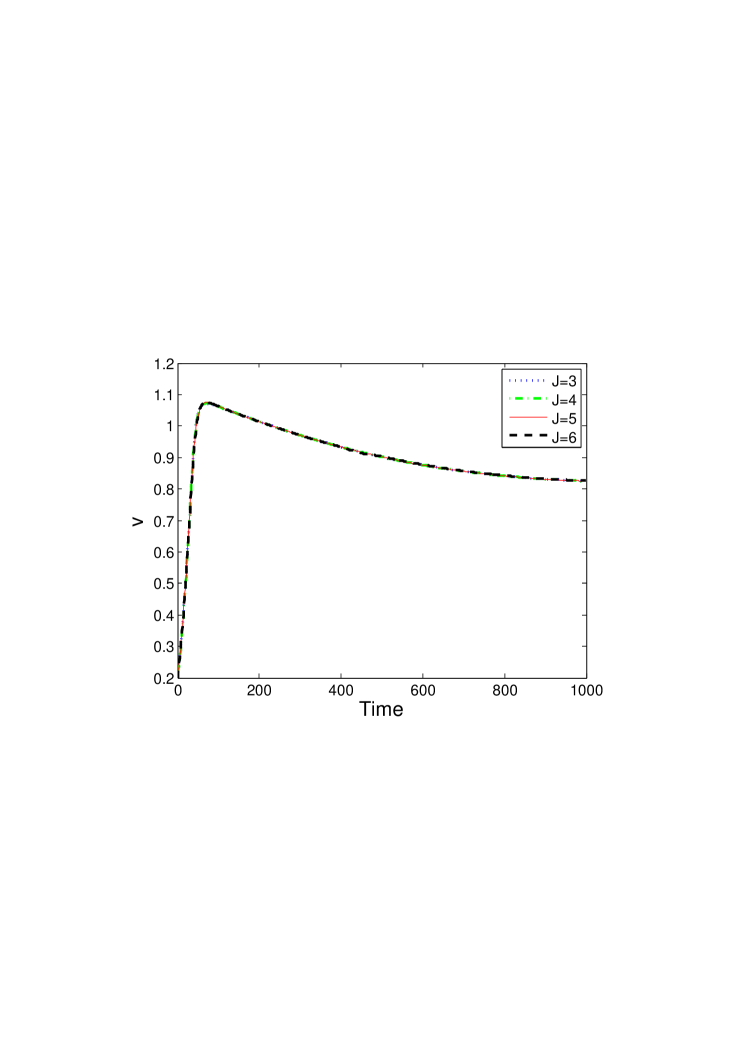
To demonstrate the power of Haar wavelet method we presented a few examples which are related to the pathological case studies in cardiac electrical activity. We solve all the examples using the above developed Haar wavelet method and calculate the absolute error also. Grid validation test or resolution level test has been done for all the problems and here we are presenting for some of the problems. From grid validation we observe that resolution level J=4𝐽4J=4 in two dimension is good enough to calculate the solution. We also compare the Haar wavelet solution with the solution obtained using the finite element method for almost all the problems. We also calculate the CPU time for Haar wavelet method and the finite element method. For all the examples, we use the GMRES solver to solve the linear system of equations obtained from the discrete problem as it is more appropriate in terms of the CPU time in comparison to the other solvers like, CGS, BICG and BICGSTAB in terms of the CPU time (see Table (5)).

Example 111. We consider the one dimensional reaction-diffusion system coupled with the ODE having homogeneous Neumann boundary. Such type of coupled systems are important because it models the problems related to the field of cardiac electrical activity of any species. We will also discuss the problem with jump discontinuity in the parameter or coefficients which is related to the problem of ischemia in cardiac tissue.

ϵvtdddx(dvdx)+kv(v0.1)(1v)kwitalic-ϵ𝑣𝑡𝑑𝑑𝑑𝑥𝑑𝑣𝑑𝑥𝑘𝑣𝑣0.11𝑣𝑘𝑤\displaystyle\epsilon\frac{\partial v}{\partial t}-d\frac{d}{dx}(\frac{dv}{dx})+kv(v-0.1)(1-v)-kw =Iapp,absentsubscript𝐼𝑎𝑝𝑝\displaystyle=I_{app}, 0x1,0tTformulae-sequence0𝑥10𝑡𝑇\displaystyle 0\leq x\leq 1,0\leq t\leq T
wt𝑤𝑡\displaystyle\frac{\partial w}{\partial t} =v2w,absent𝑣2𝑤\displaystyle=v-2w, 0x1,0tTformulae-sequence0𝑥10𝑡𝑇\displaystyle 0\leq x\leq 1,0\leq t\leq T
v(x,0)=0.2,w(x,0)𝑣𝑥00.2𝑤𝑥0\displaystyle v(x,0)=0.2,\hskip 14.22636ptw(x,0) =0.2,absent0.2\displaystyle=0.2, 0x10𝑥1\displaystyle 0\leq x\leq 1
dvdx(0,t)=0,dvdx(1,t)=0formulae-sequence𝑑𝑣𝑑𝑥0𝑡0𝑑𝑣𝑑𝑥1𝑡0\displaystyle\frac{dv}{dx}(0,t)=0,\hskip 14.22636pt\frac{dv}{dx}(1,t)=0 =0,absent0\displaystyle=0, 0tT0𝑡𝑇\displaystyle 0\leq t\leq T

where, d=0.005𝑑0.005d=0.005 and ϵ=0.01italic-ϵ0.01\epsilon=0.01.

Resolution level test for the proposed Haar wavelet method has been presented in Fig. 3.
Refer to caption
Figure 3: Resolution level test for Haar wavelet solution v𝑣v

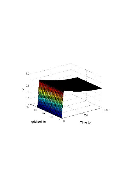
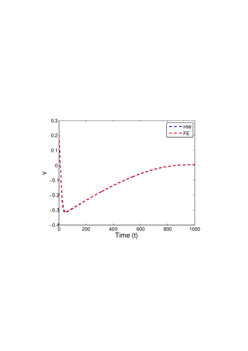
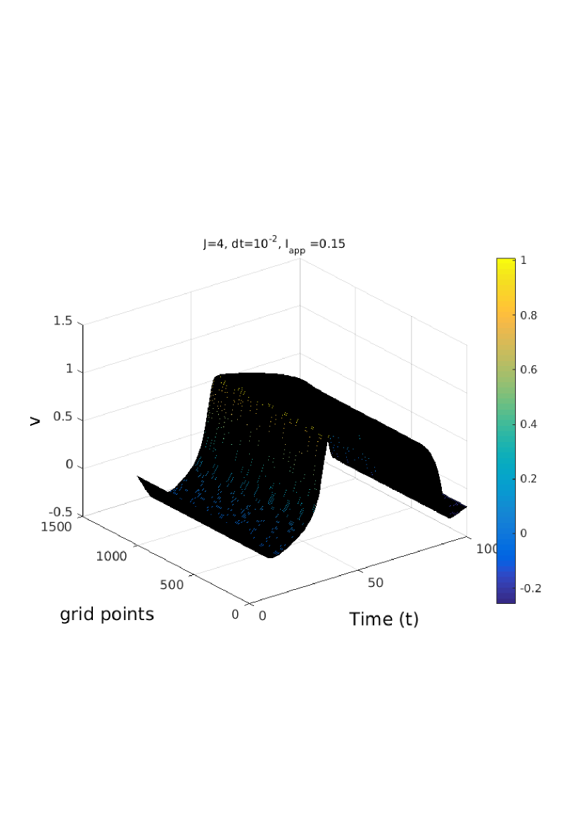
Pointwise absolute error for different time steps is shown in Table 1. Solution at dt=105,J=8formulae-sequence𝑑𝑡superscript105𝐽8dt=10^{-5},J=8 is taken as the reference solution. From the Table 1, it can be seen clearly that absolute error decreases significantly with the smaller time step size. The Haar wavelet solution for v𝑣v at the grid points is presented in Fig. 4. We also solved the same problem using the linear finite element in space and implicit-explicit (IE) Euler method in time. It is observed that the Haar wavelet solution matches with the finite element solution (Fig. 5).

x absolute error
dt=103𝑑𝑡superscript103dt=10^{-3} dt=104𝑑𝑡superscript104dt=10^{-4}
0.1406 6.4×1036.4superscript1036.4\times 10^{-3} 6.2×1046.2superscript1046.2\times 10^{-4}
0.2656 6.9×1036.9superscript1036.9\times 10^{-3} 6.085×1046.085superscript1046.085\times 10^{-4}
0.3594 8.1×1038.1superscript1038.1\times 10^{-3} 5.464×1045.464superscript1045.464\times 10^{-4}
0.4531 8.8×1038.8superscript1038.8\times 10^{-3} 5.4×1045.4superscript1045.4\times 10^{-4}
Table 1: (For example 1)Absolute Error for v𝑣v at different points of the domain when J=8𝐽8J=8 and T=1.
Refer to caption
Figure 4: (for example1) Haar wavelet solution for v𝑣v. Iapp=0.3subscript𝐼𝑎𝑝𝑝0.3I_{app}=0.3.
Refer to caption
Figure 5: FE and HW solution at x=0.5. Iapp=0subscript𝐼𝑎𝑝𝑝0I_{app}=0, J=5, dt=103𝑑𝑡superscript103dt=10^{-3} and T=1.

From Fig. 5 we can see that when Iapp=0subscript𝐼𝑎𝑝𝑝0I_{app}=0, variable v𝑣v goes to the resting state without shooting up. But as we provide Iapp=0.3subscript𝐼𝑎𝑝𝑝0.3I_{app}=0.3, the solution v𝑣v shoot up from the initial state and then it goes down slowly to the stabilizing state. This type of problems models pathological phenomena like FitzHugh Nagumo (FHN) model in cardiac electrical activity, which is the reduced ionic model of animal.

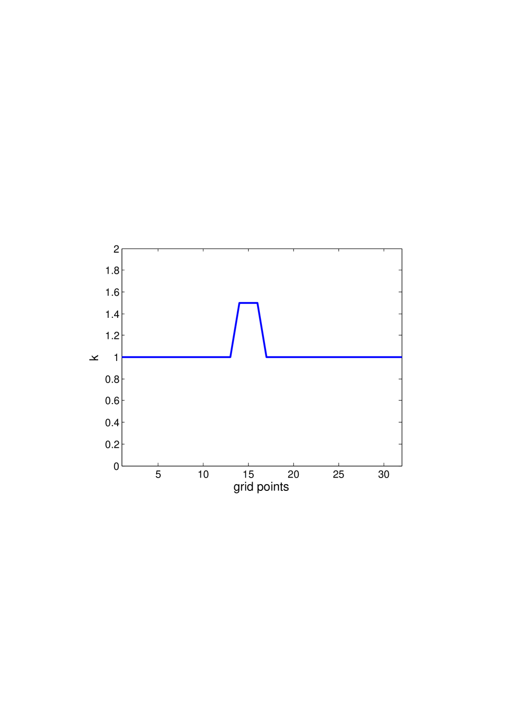
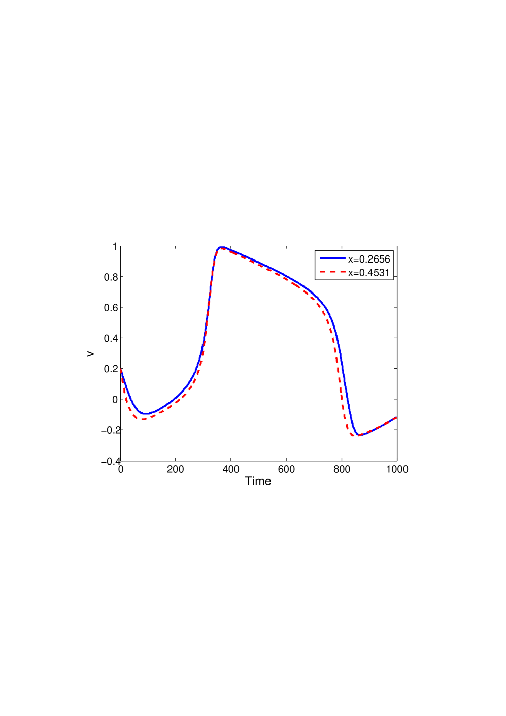
Next, we consider the same problem but with a jump discontinuity in the parameter k𝑘k, drawn in Fig. 6(a) which creates the local ischemia in a cardiac tissue. We calculate the solution v𝑣v at the points, as a sample, in Fig (6(b)) we present the solution corresponding to the points x=0.2656𝑥0.2656x=0.2656 and x=0.4531𝑥0.4531x=0.4531, which lie outside and inside the jump region respectively. The absence of any spurious oscillation in the solution presented in Fig. 6(b) indicated that Haar wavelets efficiently handle this jump discontinuity.
Refer to caption
(a)
Refer to caption
(b)
Figure 6: (a) parameter k𝑘k, (b) Corresponding Haar wavelet solution v𝑣v at the points falling inside and outside the jump region. Iapp=0.15subscript𝐼𝑎𝑝𝑝0.15I_{app}=0.15

Example 222

We will consider the two dimensional problems which are important in the field of cardiac electrophysiology. We will calculate the transmembrane potential in the heart which is important to know the functionality of the heart. We will solve the problem having jump discontinuity in any parameter or coefficients using the Haar wavelets.

ϵvtdiv(Dv)+kv(v0.1)(1v)kw=Iapp,italic-ϵ𝑣𝑡𝑑𝑖𝑣𝐷𝑣𝑘𝑣𝑣0.11𝑣𝑘𝑤subscript𝐼𝑎𝑝𝑝\displaystyle\epsilon\frac{\partial v}{\partial t}-div(D\nabla v)+kv(v-0.1)(1-v)-kw=I_{app}, 0x,y1,0tTformulae-sequence0𝑥formulae-sequence𝑦10𝑡𝑇\displaystyle 0\leq x,y\leq 1,0\leq t\leq T
wt=v2w,𝑤𝑡𝑣2𝑤\displaystyle\frac{\partial w}{\partial t}=v-2w, 0x,y1,0tTformulae-sequence0𝑥formulae-sequence𝑦10𝑡𝑇\displaystyle 0\leq x,y\leq 1,0\leq t\leq T
v(x,0)=0.2,w(x,0)=0.2,formulae-sequence𝑣𝑥00.2𝑤𝑥00.2\displaystyle v(x,0)=0.2,\hskip 14.22636ptw(x,0)=0.2, 0x,y1formulae-sequence0𝑥𝑦1\displaystyle 0\leq x,y\leq 1
dvdx(0,y,t)=0,𝑑𝑣𝑑𝑥0𝑦𝑡0\displaystyle\frac{dv}{dx}(0,y,t)=0, 0tT0𝑡𝑇\displaystyle 0\leq t\leq T
dvdx(1,y,t)=0,𝑑𝑣𝑑𝑥1𝑦𝑡0\displaystyle\frac{dv}{dx}(1,y,t)=0, 0tT0𝑡𝑇\displaystyle 0\leq t\leq T
dvdy(x,0,t)=0,𝑑𝑣𝑑𝑦𝑥0𝑡0\displaystyle\frac{dv}{dy}(x,0,t)=0, 0tT0𝑡𝑇\displaystyle 0\leq t\leq T
dvdy(x,1,t)=0,𝑑𝑣𝑑𝑦𝑥1𝑡0\displaystyle\frac{dv}{dy}(x,1,t)=0, 0tT0𝑡𝑇\displaystyle 0\leq t\leq T

where D=[1.2e3002.5562e4]𝐷matrix1.2𝑒3002.5562𝑒4D=\begin{bmatrix}1.2e{-3}&0\\ 0&2.5562e{-4}\end{bmatrix}, ϵ=0.01italic-ϵ0.01\epsilon=0.01 and Iapp=0.15subscript𝐼𝑎𝑝𝑝0.15I_{app}=0.15.

First of all the grid validation of the proposed algorithm for this problem is presented in Fig. 7 which clearly shows the accuracy of the solution at the different resolution level. So, resolution level J=4𝐽4J=4 is good enough to calculate the results.
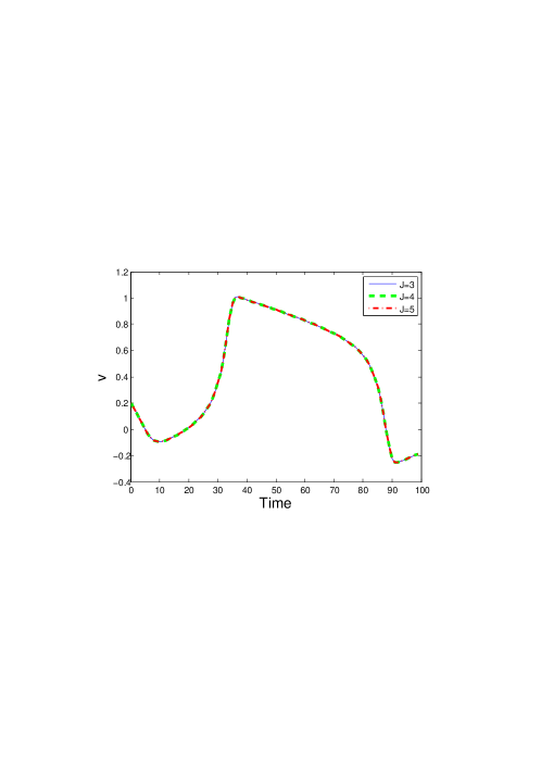
Refer to caption
Figure 7: Resolution level test for Haar wavelet solution v𝑣v

Absolute error for different time steps is shown in Table 2. Solution at dt=105,J=6formulae-sequence𝑑𝑡superscript105𝐽6dt=10^{-5},J=6 is taken as the reference solution. From the Table 2 it can be seen clearly that absolute error decreases seriously with the smaller time step size.

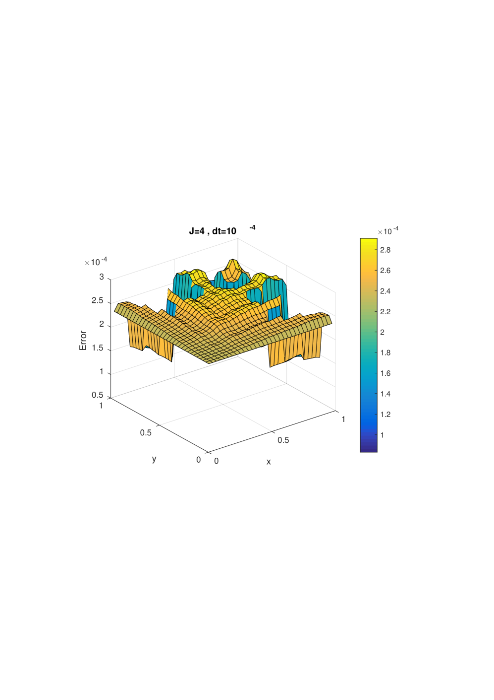
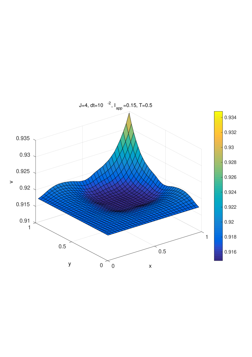
Pointwise absolute error of the Haar wavelet solution v𝑣v is presented in Fig.8(a). Haar wavelet solution in surface is shown in Fig. 9(a) and Fig. 9(b) respectively. We also solved the same problem using the linear finite element in space and implicit-explicit (IE) Euler method in time. Haar wavelet solution matches with the finite element solution as shown in Fig. 8(b).

Maximum absolute error
dt=102𝑑𝑡superscript102dt=10^{-2} dt=103𝑑𝑡superscript103dt=10^{-3} dt=104𝑑𝑡superscript104dt=10^{-4}
1.7×1021.7superscript1021.7\times 10^{-2} 1.9×1031.9superscript1031.9\times 10^{-3} 8.3×1058.3superscript1058.3\times 10^{-5}
Table 2: Maximum Absolute Error (for example 2) of v𝑣v when J=6𝐽6J=6 and T=0.5, k=1.
Refer to caption
(a)
Refer to caption
(b)
Figure 8: (a) Numerical error at J=6 and T=0.5 and dt=104𝑑𝑡superscript104dt=10^{-4}, (b) FE and HW solution comparison at J=5 and T=1 and dt=104𝑑𝑡superscript104dt=10^{-4}, k=1𝑘1k=1.
Refer to caption
(a)
Refer to caption
(b)
Figure 9: (a) Surface plot, Haar wavelet solution in 2D, (b)Haar wavelet solution in 2D

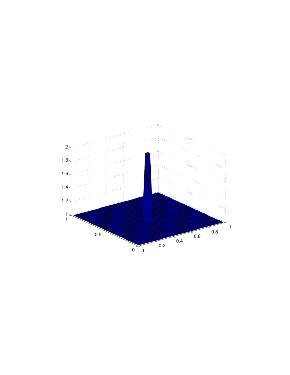
Now, if the parameter k𝑘k in the above equation have jump discontinuity at some places in the domain, as shown in Fig. 10(a). This jump parameter models the local ischemia in the heart tissue. It is important to calculate the transmembrane potential with this ischemia to know the change in electrical activity of the heart.

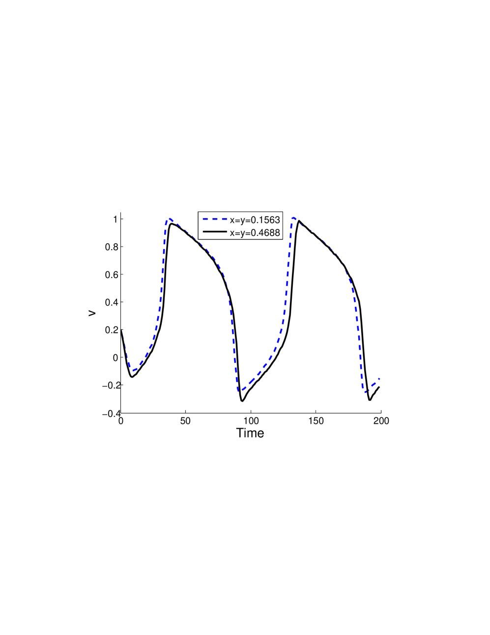
The solution v𝑣v corresponding to this value of the parameter k𝑘k at the points (0.1563,0.1563) (lies outside the jump region) and (0.4688,0.4688) (lies within the jump region of the domain) are drawn in Fig. 10(b). There is no oscillation in the solution with discontinuity is noticed also the behavior of the solution clearly depict that Haar wavelets handle the jump discontinuity in the parameter k𝑘k.

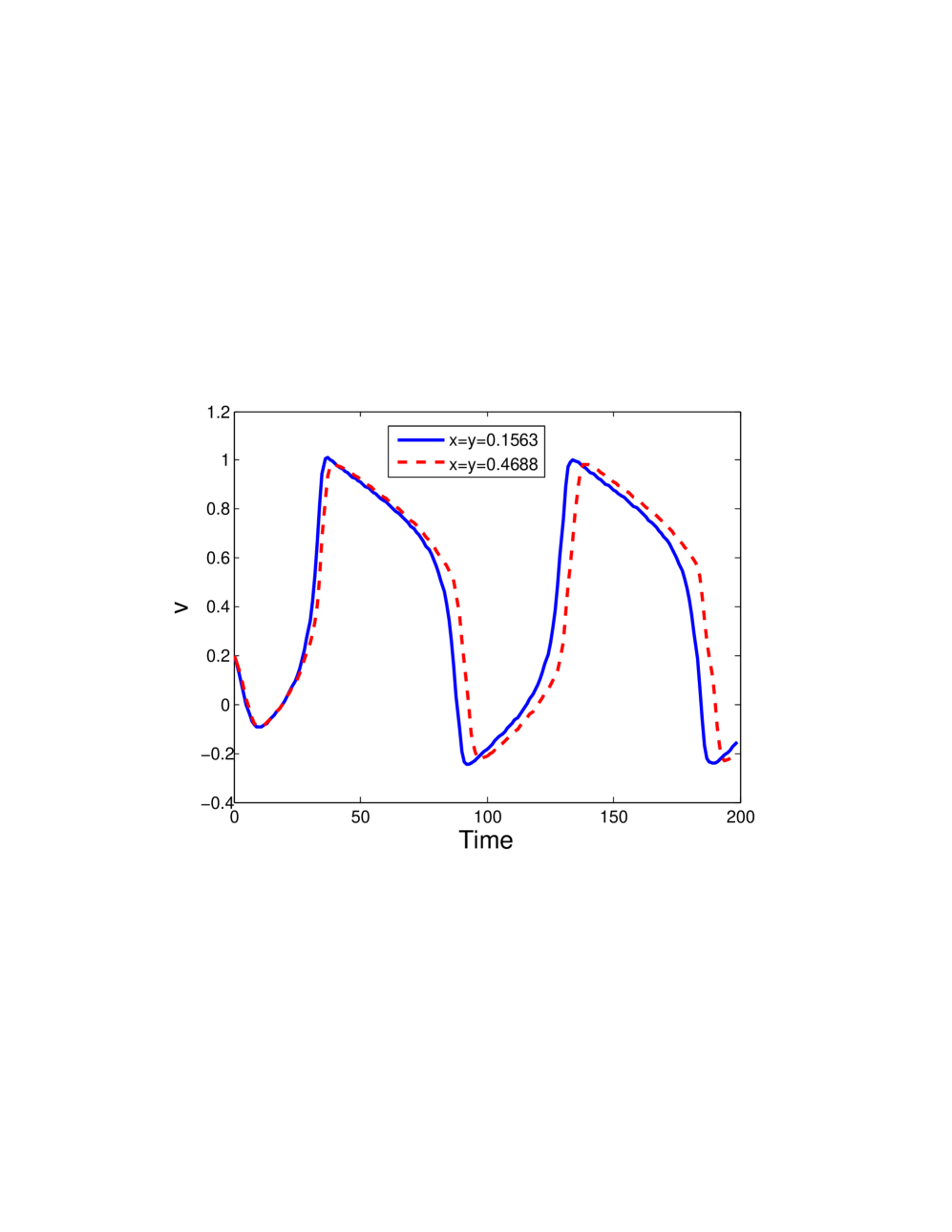
Again, if the discontinuity is in the parameter ϵitalic-ϵ\epsilon of the model equation, like drawn in Fig. 11(a). The solution v𝑣v corresponding to this value of the parameter ϵitalic-ϵ\epsilon at the points (0.1563,0.1563) and (0.4688,0.4688) lies outside and inside the jump region respectively in the domain are presented in Fig. 11(b). Behavior of the solution with discontinuity in this parameter conclude that the ϵitalic-ϵ\epsilon discontinuity is automatically handled by the Haar wavelets.
Refer to caption
(a)
Refer to caption
(b)
Figure 10: (a) k𝑘k parameter value, (b) Solution for v𝑣v with jump discontinuity in k𝑘k parameter.
Refer to caption
(a)
Refer to caption
(b)
Figure 11: (a) ϵitalic-ϵ\epsilon parameter value, (b) Corresponding solution v𝑣v.

Example 333

We will consider the example which is important in the field of cardiac electrophysiology. This model includes only inward and outward current. It contains four time constants, for the four phases of cardiac action potential: initial, plateau, decay and recovery. We will solve the problem having multiple jump discontinuity in any of these parameter using the Haar wavelets.

vtdiv(Dv)+f(v,w)=Iapp,𝑣𝑡𝑑𝑖𝑣𝐷𝑣𝑓𝑣𝑤subscript𝐼𝑎𝑝𝑝\displaystyle\frac{\partial v}{\partial t}-div(D\nabla v)+f(v,w)=I_{app}, 0x,y1,0tTformulae-sequence0𝑥formulae-sequence𝑦10𝑡𝑇\displaystyle 0\leq x,y\leq 1,0\leq t\leq T
wt=G(v,w),𝑤𝑡𝐺𝑣𝑤\displaystyle\frac{\partial w}{\partial t}=G(v,w), 0x,y1,0tTformulae-sequence0𝑥formulae-sequence𝑦10𝑡𝑇\displaystyle 0\leq x,y\leq 1,0\leq t\leq T
v(x,0)=0.2,w(x,0)=0.2,formulae-sequence𝑣𝑥00.2𝑤𝑥00.2\displaystyle v(x,0)=0.2,\hskip 14.22636ptw(x,0)=0.2, 0x,y1formulae-sequence0𝑥𝑦1\displaystyle 0\leq x,y\leq 1
dvdx(0,y,t)=0,𝑑𝑣𝑑𝑥0𝑦𝑡0\displaystyle\frac{dv}{dx}(0,y,t)=0, 0tT0𝑡𝑇\displaystyle 0\leq t\leq T
dvdx(1,y,t)=0,𝑑𝑣𝑑𝑥1𝑦𝑡0\displaystyle\frac{dv}{dx}(1,y,t)=0, 0tT0𝑡𝑇\displaystyle 0\leq t\leq T
dvdy(x,0,t)=0,𝑑𝑣𝑑𝑦𝑥0𝑡0\displaystyle\frac{dv}{dy}(x,0,t)=0, 0tT0𝑡𝑇\displaystyle 0\leq t\leq T
dvdy(x,1,t)=0,𝑑𝑣𝑑𝑦𝑥1𝑡0\displaystyle\frac{dv}{dy}(x,1,t)=0, 0tT0𝑡𝑇\displaystyle 0\leq t\leq T

where,

f(v,w)=wτinv2(v1)vτout,𝑓𝑣𝑤𝑤subscript𝜏𝑖𝑛superscript𝑣2𝑣1𝑣subscript𝜏𝑜𝑢𝑡\displaystyle f(v,w)=-\frac{w}{\tau_{in}}v^{2}(v-1)-\frac{v}{\tau_{out}},
G(u,w)={1wτopenvugate,wτclosev>ugate.𝐺𝑢𝑤cases1𝑤subscript𝜏𝑜𝑝𝑒𝑛𝑣subscript𝑢𝑔𝑎𝑡𝑒𝑤subscript𝜏𝑐𝑙𝑜𝑠𝑒𝑣subscript𝑢𝑔𝑎𝑡𝑒\displaystyle G(u,w)=\begin{cases}\frac{1-w}{\tau_{open}}&v\leq u_{gate},\\ \frac{-w}{\tau_{close}}&v>u_{gate}.\\ \end{cases}

D=[1.2e3002.5562e4]𝐷matrix1.2𝑒3002.5562𝑒4D=\begin{bmatrix}1.2e{-3}&0\\ 0&2.5562e{-4}\end{bmatrix}, and Iapp={20Nt100,0o.w.subscript𝐼𝑎𝑝𝑝cases20𝑁𝑡1000formulae-sequence𝑜𝑤I_{app}=\begin{cases}20&Nt\leq 100,\\ 0&o.w.\\ \end{cases}.

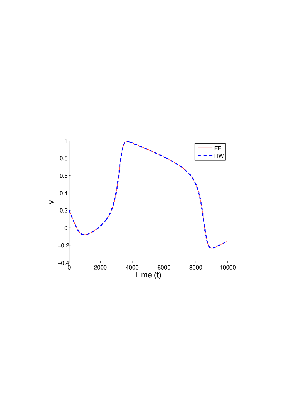
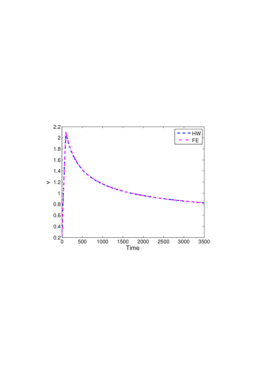
The solution of this model with the above proposed HW matches with the FE solution, shown in Fig. 12.
Refer to caption
Figure 12: FE and HW solution comparison at J=4 and T=3.5 and dt=103𝑑𝑡superscript103dt=10^{-3}.

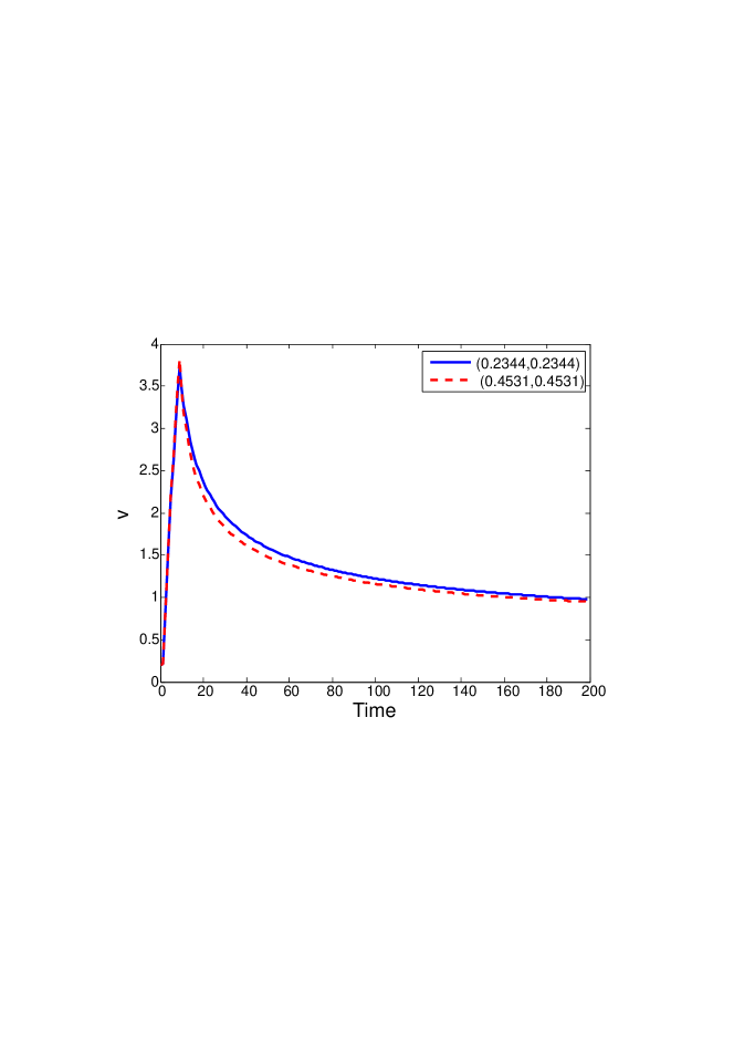
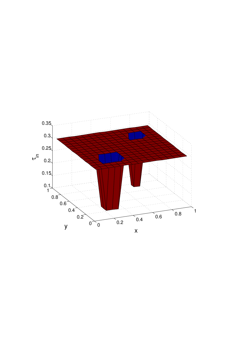
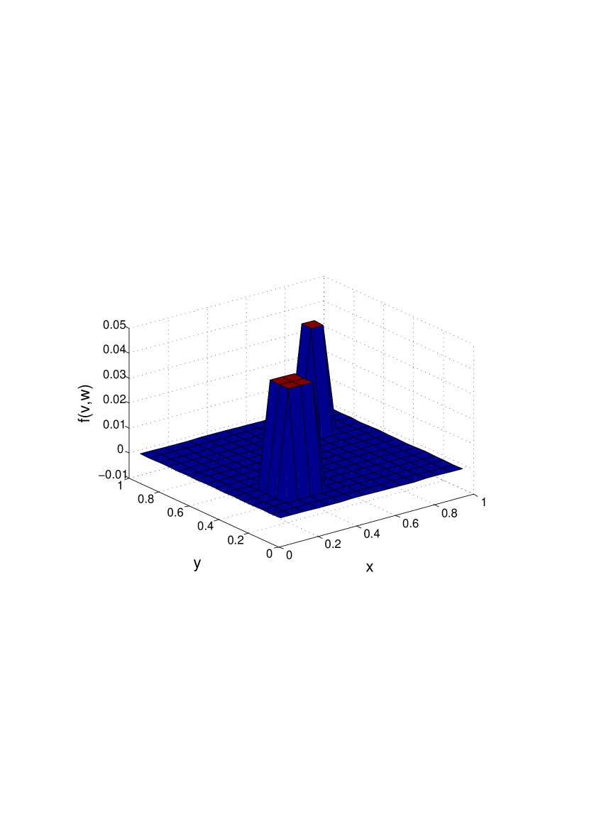
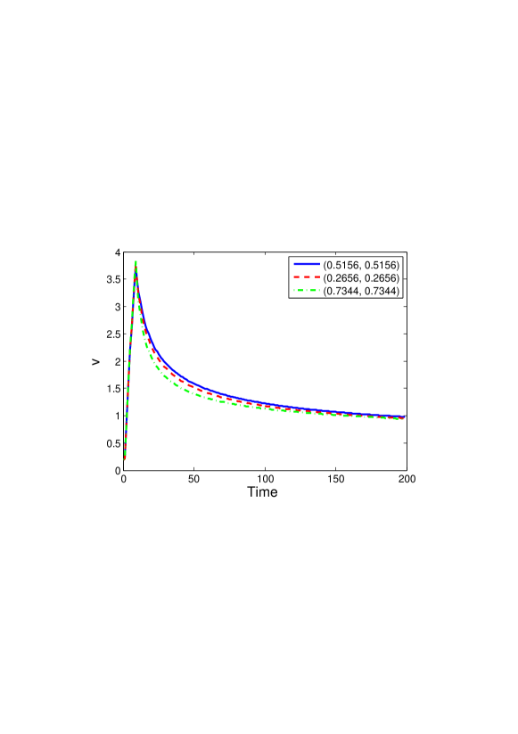
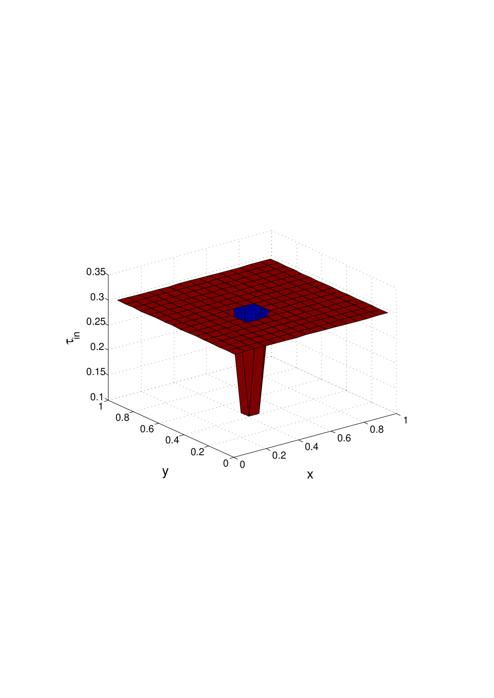
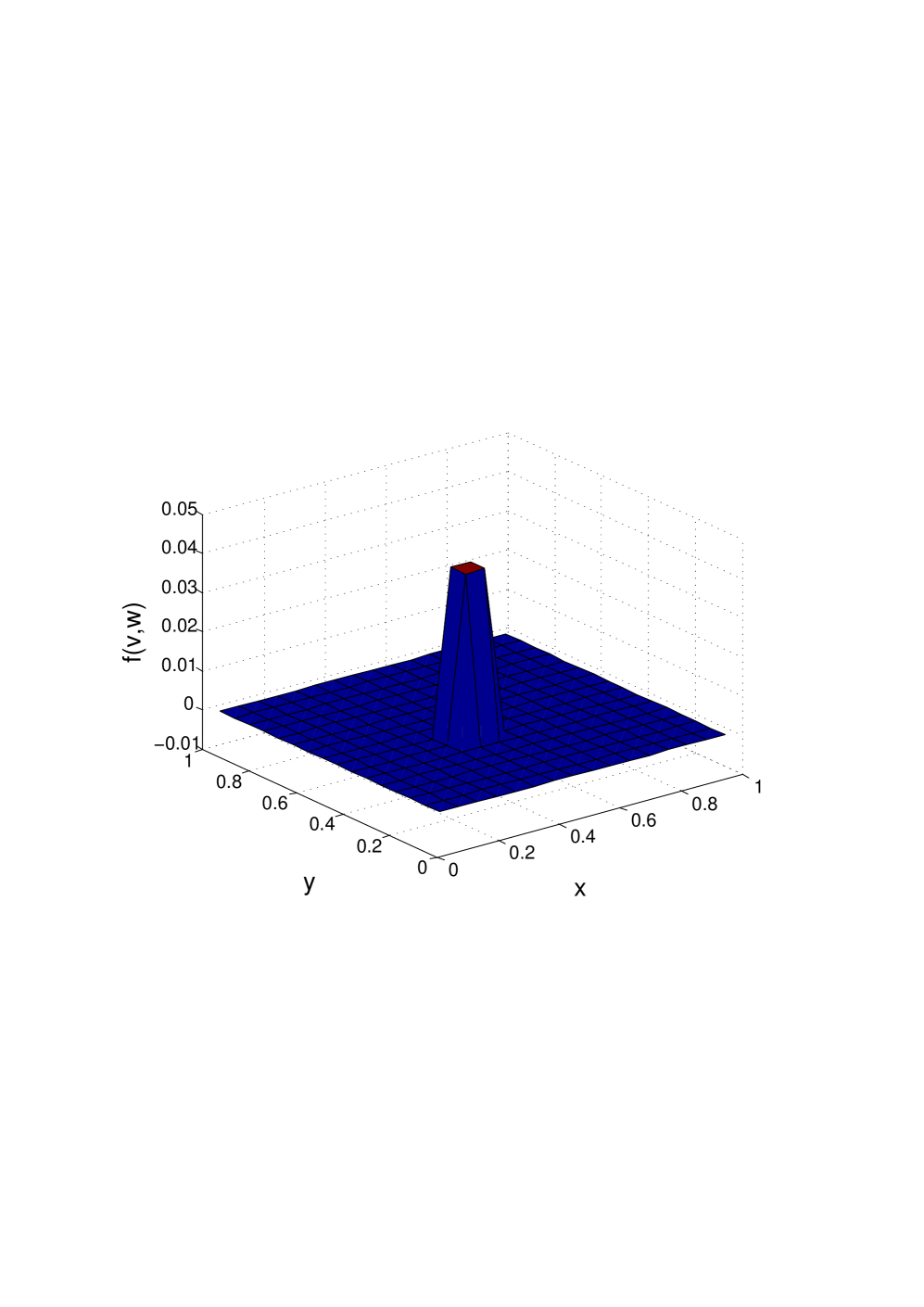
Now, if the parameter τinsubscript𝜏𝑖𝑛\tau_{in} in the above equation have jump discontinuity at some places in the domain, as shown in Fig. 13(a) and Fig. 15(a), the corresponding function Iion(v,w)subscript𝐼𝑖𝑜𝑛𝑣𝑤I_{ion}(v,w) will also be discontinuous, shown in Fig. 13(b) and 15(b). This discontinuity is automatically handled using Haar wavelets. The solution v𝑣v corresponding to τinsubscript𝜏𝑖𝑛\tau_{in} in Fig. 13(a) at the points (0.2344,0.2344) and (0.4531,0.4531), lie outside and inside the jump region of the domain are shown in Fig. 14. Now, the solution v𝑣v corresponding to τinsubscript𝜏𝑖𝑛\tau_{in} in Fig. 15(a) at the points (0.2656, 0.2656), (0.5156, 0.5156) and (0.7344, 0.7344) are presented in Fig. 16. From these Figures, we can clearly see that Haar wavelets automatically handle the multiple jumps in the parameter τinsubscript𝜏𝑖𝑛\tau_{in}. This clearly describes the power of using Haar wavelets.

This type of single or multiple jump discontinuity problems are useful to calculate the effect of ischemia in the cardiac electrical activity in a tissue with single or multiple ischemic subregions. In such type of problems local ischemia is handled by changing the value of the corresponding parameters into the model at these ischemic subregions only. Thus, Haar wavelet method is a computationally effective tool to solve such types of pathological problems.
Refer to caption
(a)
Refer to caption
(b)
Figure 13: (a)τinsubscript𝜏𝑖𝑛\tau_{in} parameter value, (b) Function f(v,w)𝑓𝑣𝑤f(v,w).
Refer to caption
Figure 14: Solution v𝑣v with jump discontinuity in τinsubscript𝜏𝑖𝑛\tau_{in} parameter.
Refer to caption
(a)
Refer to caption
(b)
Figure 15: (a) τinsubscript𝜏𝑖𝑛\tau_{in} parameter value with jump discontinuity at two regions, (b) Corresponding function f(v,w)𝑓𝑣𝑤f(v,w).
Refer to caption
Figure 16: Solution v𝑣v with jump discontinuity at two places in τinsubscript𝜏𝑖𝑛\tau_{in} parameter.

Comparison of the computation time of finite element solution and the Haar wavelet solution for 2D model in example 2 and example 3 is presented in Table 3. Clearly, from the table, the haar wavelet method reduces the computational cost in comparison of FEM.

J dt FEM CPU time (sec) HW CPU time (sec)
Example 2 3 (256 grid) 102superscript10210^{-2} 2.06464 1.690459
4 (1024 grid) 102superscript10210^{-2} 7.30766 6.40874
Example 3 3 (256 grid) 102superscript10210^{-2} 2.94036 1.527416
4 (1024 grid) 102superscript10210^{-2} 9.84829 5.342718
Table 3: CPU time 2D

Example 4

We will solve the following Monodomain cardiac tissue level model with the complex non-linear Hodgkin-Huxely ionic model Hodgkin and Huxley (1952) using the above developed Haar wavelet method.

vtdiv(D(x)v)+Iion(v,w)𝑣𝑡𝑑𝑖𝑣𝐷𝑥𝑣subscript𝐼𝑖𝑜𝑛𝑣𝑤\displaystyle\frac{\partial v}{\partial t}-div(D(x)\nabla v)+I_{ion}(v,w) =Iapp,absentsubscript𝐼𝑎𝑝𝑝\displaystyle=I_{app}, xΩ,0tTformulae-sequence𝑥Ω0𝑡𝑇\displaystyle x\in\Omega,0\leq t\leq T
wtg(v,w)𝑤𝑡𝑔𝑣𝑤\displaystyle\frac{\partial w}{\partial t}-g(v,w) =0,absent0\displaystyle=0, xΩ,0tTformulae-sequence𝑥Ω0𝑡𝑇\displaystyle x\in\Omega,0\leq t\leq T
v(x,0)=v0(x,0),w(x,0)𝑣𝑥0subscript𝑣0𝑥0𝑤𝑥0\displaystyle v(x,0)=v_{0}(x,0),\hskip 14.22636ptw(x,0) =wi,0(x,0),absentsubscript𝑤𝑖0𝑥0\displaystyle=w_{i,0}(x,0), xΩ𝑥Ω\displaystyle x\in\Omega
nTD(x)vsuperscript𝑛𝑇𝐷𝑥𝑣\displaystyle n^{T}D(x)\nabla v =0,absent0\displaystyle=0, xΩ,0tTformulae-sequence𝑥Ω0𝑡𝑇\displaystyle x\in\partial\Omega,0\leq t\leq T

where, Iappsubscript𝐼𝑎𝑝𝑝I_{app} is the applied stimulus and D(x)𝐷𝑥D(x) is the conductivity tensor defined as:

D(x)=σtI+(σlσt)bl(x)blt(x)withσs=l~σsi1+l~,s=l,t,n.formulae-sequence𝐷𝑥subscript𝜎𝑡𝐼subscript𝜎𝑙subscript𝜎𝑡subscript𝑏𝑙𝑥superscriptsubscript𝑏𝑙𝑡𝑥𝑤𝑖𝑡subscript𝜎𝑠~𝑙subscriptsuperscript𝜎𝑖𝑠1~𝑙𝑠𝑙𝑡𝑛\displaystyle D(x)={\sigma_{t}}I+({\sigma_{l}}-{\sigma_{t}})b_{l}(x){b_{l}}^{t}(x)\hskip 8.53581ptwith\hskip 8.53581pt\sigma_{s}=\frac{\widetilde{l}\sigma^{i}_{s}}{1+\widetilde{l}},s=l,t,n.

g(v,w)𝑔𝑣𝑤g(v,w) an Iion(v,w)subscript𝐼𝑖𝑜𝑛𝑣𝑤I_{ion}(v,w) are given by the models at the cell level, called ionic models. Here, we are choosing the Hodgkin Huxely ionic model.

Hodking and Huxely in 1952 modeled an ionic model to calculate the action potential in a squid giant axon. In this model, sodium and potassium ionic channels and hence corresponding two separate ionic currents are taken into account. All other small ionic currents are lumped into the leakage current. The model equation is given as follows

Iion=gNam3h(vENa)+gKn4(vEK)+gL(vEL),subscript𝐼𝑖𝑜𝑛subscript𝑔𝑁𝑎superscript𝑚3𝑣subscript𝐸𝑁𝑎subscript𝑔𝐾superscript𝑛4𝑣subscript𝐸𝐾subscript𝑔𝐿𝑣subscript𝐸𝐿\displaystyle I_{ion}=g_{Na}m^{3}h(v-E_{Na})+g_{K}n^{4}(v-E_{K})+g_{L}(v-E_{L}), (31)

where, gNasubscript𝑔𝑁𝑎g_{Na} and gKsubscript𝑔𝐾g_{K} are the maximal conductances corresponding to their membrane which depends on the voltage and time, ENa,EK,ELsubscript𝐸𝑁𝑎subscript𝐸𝐾subscript𝐸𝐿E_{Na},E_{K},E_{L} are the corresponding ion resting potentials. Iappsubscript𝐼𝑎𝑝𝑝I_{app} is the externally applied current. m𝑚m, hh and n𝑛n are the gating variables and the dynamics of each of the gating variables is described by the ordinary differential equation:

dwdt=αw(1w)βw,w=m,h,n,formulae-sequence𝑑𝑤𝑑𝑡subscript𝛼𝑤1𝑤subscript𝛽𝑤𝑤𝑚𝑛\displaystyle\frac{dw}{dt}=\alpha_{w}(1-w)-\beta_{w},\hskip 8.53581ptw=m,h,n, (32)

where, αwsubscript𝛼𝑤\alpha_{w} and βwsubscript𝛽𝑤\beta_{w} are the rates depends upon the membrane voltage.

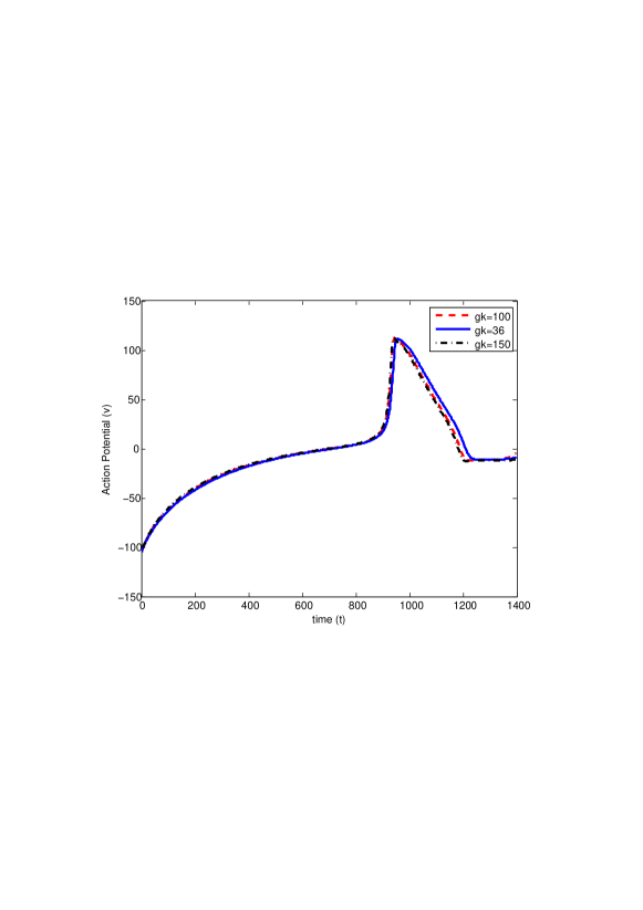
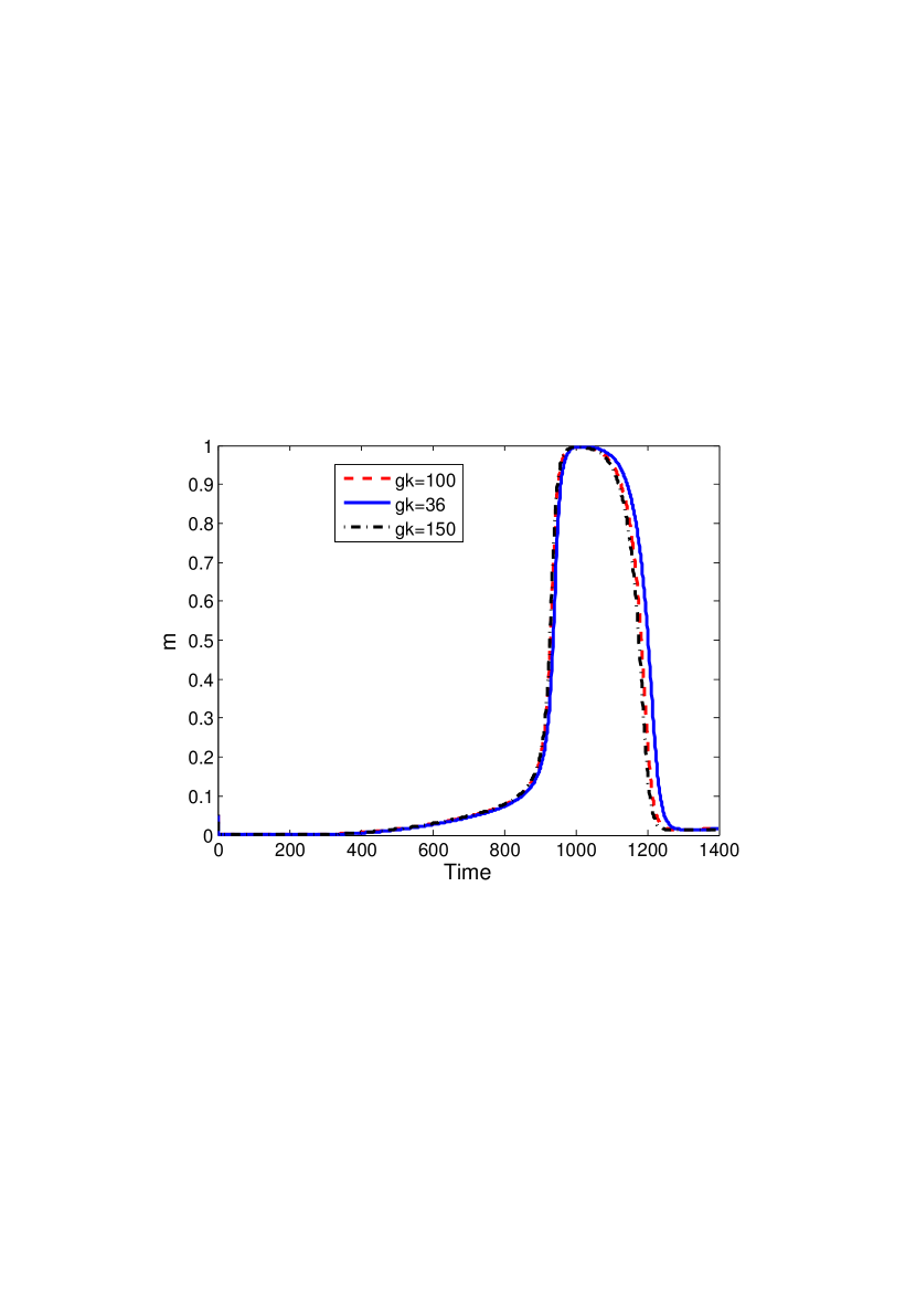
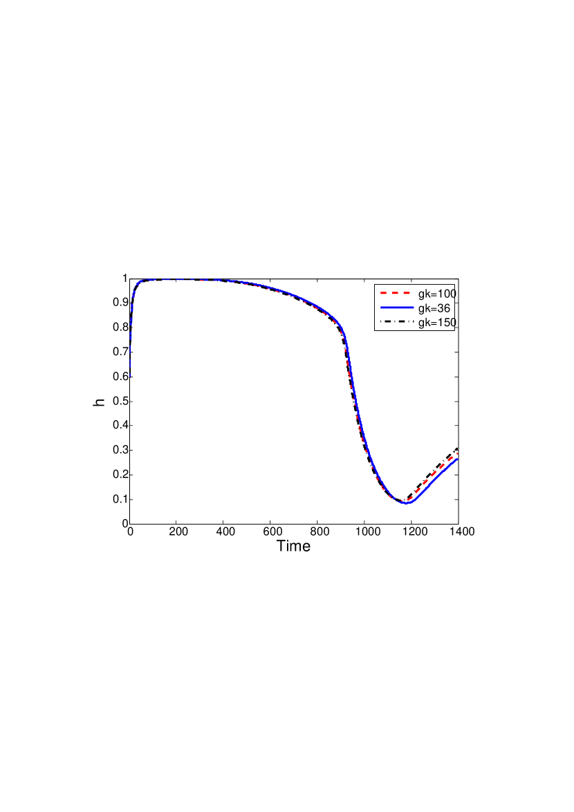
Here, the conductivity of potassium ion gKsubscript𝑔𝐾g_{K} depends on the voltage and time. If we change this parameter value membrane potential or the action potential will also change in the tissue. Action potential and the gating variables for the different value of the parameter is presented in Fig. 17, 18(a) and 18(b).

The jump discontinuity in the parameter gKsubscript𝑔𝐾g_{K} and hence in Iionsubscript𝐼𝑖𝑜𝑛I_{ion} is handled by the Haar wavelets.

Refer to caption
Figure 17: Action Potential for HH model
Refer to caption
(a)
Refer to caption
(b)
Figure 18: (a)m gate, (b) h gate.

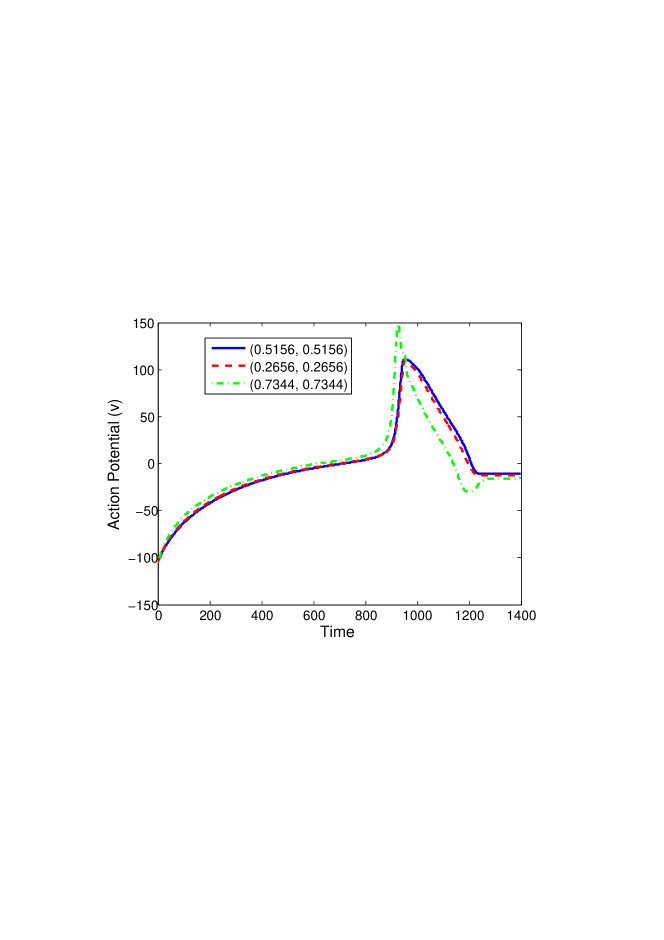
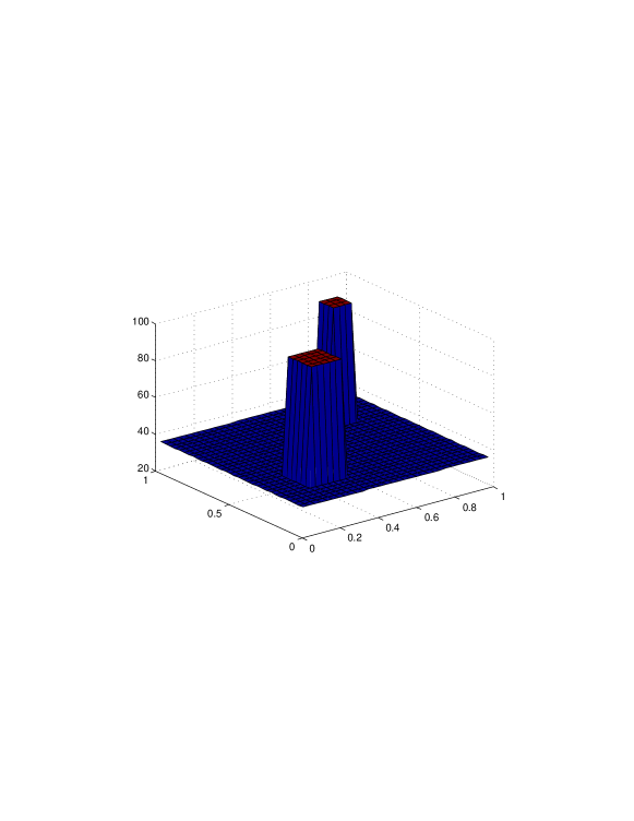
Now, we are choosing the parameter gksubscript𝑔𝑘g_{k} value having jump discontinuity at the two subdomains of the domain, as shown in Fig. 19. The corresponding function Iion(v,w)subscript𝐼𝑖𝑜𝑛𝑣𝑤I_{ion}(v,w) will also be discontinuous in the corresponding subdomains. The solution v𝑣v corresponding to this gksubscript𝑔𝑘g_{k} at the points (0.2156, 0.2156), (0.5156, 0.5156) and (0.7344, 0.7344) is presented in Fig. 20.
Refer to caption
Figure 19: gKsubscript𝑔𝐾g_{K} parameter value having jump discontinuity at two places,
Refer to caption
Figure 20: Action Potential for HH model gKsubscript𝑔𝐾g_{K} parameter value having jump discontinuity at two places.

Example 555

We will consider the three dimensional example which is important in the field of cardiac electrophysiology. This model includes only inward and outward current. It contains four time constants, for the four phases of cardiac action potential: initial, plateau, decay and recovery. We will solve the problem having jump discontinuity in any of these parameter using the Haar wavelets.

vt(d112vx2+d222vy2+d332vz2)+Iion𝑣𝑡subscript𝑑11superscript2𝑣superscript𝑥2subscript𝑑22superscript2𝑣superscript𝑦2subscript𝑑33superscript2𝑣superscript𝑧2subscript𝐼𝑖𝑜𝑛\displaystyle\frac{\partial v}{\partial t}-\bigg{(}d_{11}\frac{\partial^{2}v}{\partial x^{2}}+d_{22}\frac{\partial^{2}v}{\partial y^{2}}+d_{33}\frac{\partial^{2}v}{\partial z^{2}}\bigg{)}+I_{ion} =Iapp,absentsubscript𝐼𝑎𝑝𝑝\displaystyle=I_{app}, 0x,y,z1,0tTformulae-sequence0𝑥𝑦formulae-sequence𝑧10𝑡𝑇\displaystyle 0\leq x,y,z\leq 1,0\leq t\leq T
wt𝑤𝑡\displaystyle\frac{\partial w}{\partial t} =v2w,absent𝑣2𝑤\displaystyle=v-2w, 0x,y,z1,0tTformulae-sequence0𝑥𝑦formulae-sequence𝑧10𝑡𝑇\displaystyle 0\leq x,y,z\leq 1,0\leq t\leq T
v(x,y,z,0)=0.2,w(x,y,z,0)𝑣𝑥𝑦𝑧00.2𝑤𝑥𝑦𝑧0\displaystyle v(x,y,z,0)=0.2,\hskip 14.22636ptw(x,y,z,0) =0.2,absent0.2\displaystyle=0.2, 0x,y,z1formulae-sequence0𝑥𝑦𝑧1\displaystyle 0\leq x,y,z\leq 1

with Neumann boundary conditions in v𝑣v. where,

Iion=wτinu2(u1)uτoutsuperscript𝐼𝑖𝑜𝑛𝑤subscript𝜏𝑖𝑛superscript𝑢2𝑢1𝑢subscript𝜏𝑜𝑢𝑡\displaystyle I^{ion}=-\frac{w}{\tau_{in}}u^{2}(u-1)-\frac{u}{\tau_{out}}
G(u,w)={1wτopenuugate,wτcloseu>ugate.𝐺𝑢𝑤cases1𝑤subscript𝜏𝑜𝑝𝑒𝑛𝑢subscript𝑢𝑔𝑎𝑡𝑒𝑤subscript𝜏𝑐𝑙𝑜𝑠𝑒𝑢subscript𝑢𝑔𝑎𝑡𝑒\displaystyle G(u,w)=\begin{cases}\frac{1-w}{\tau_{open}}&u\leq u_{gate},\\ \frac{-w}{\tau_{close}}&u>u_{gate}.\\ \end{cases}

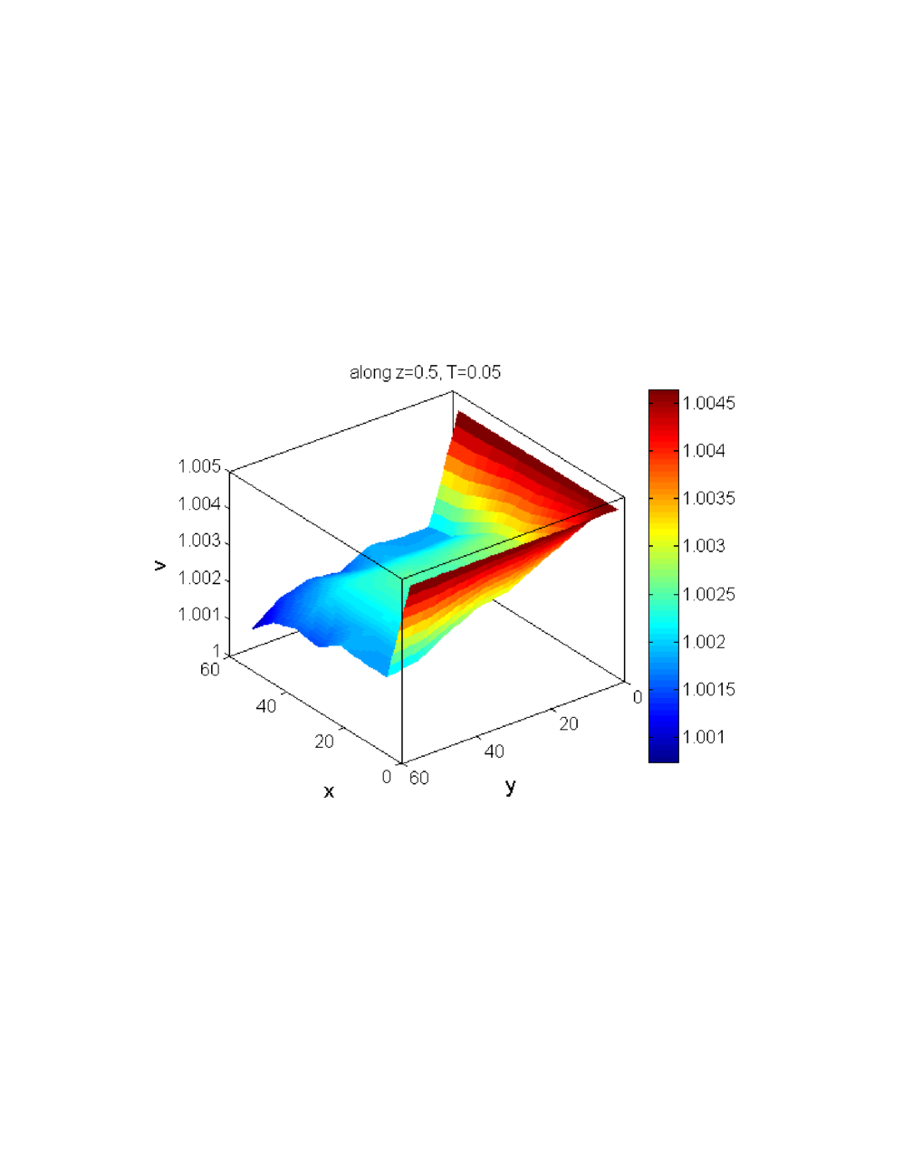
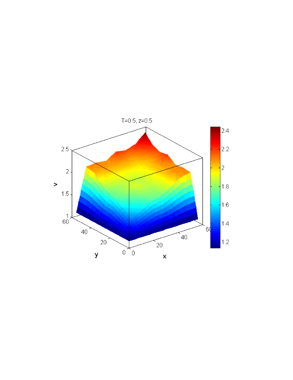
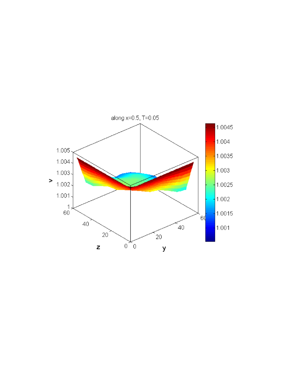
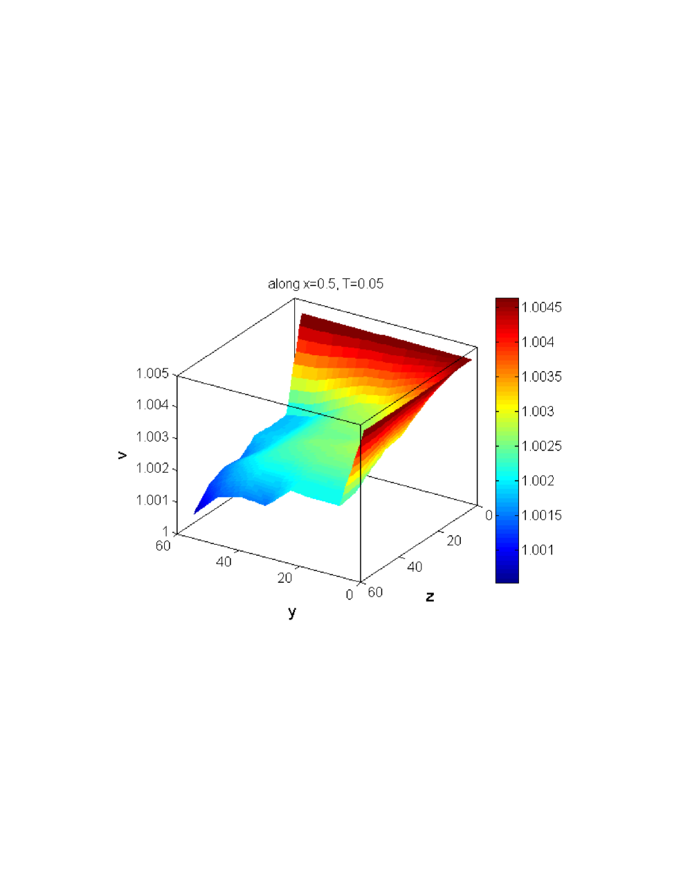
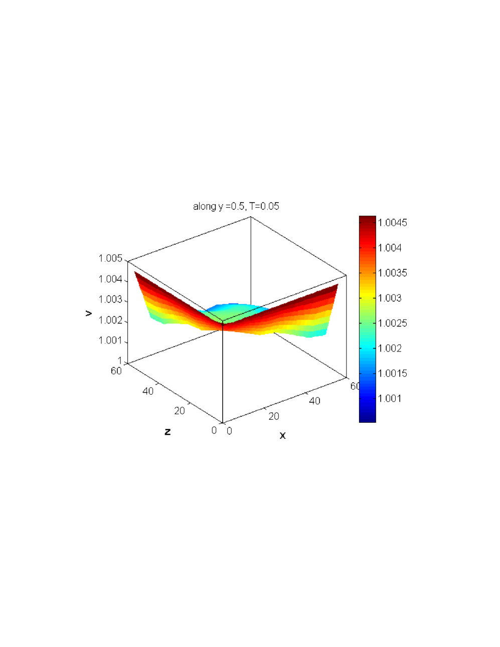
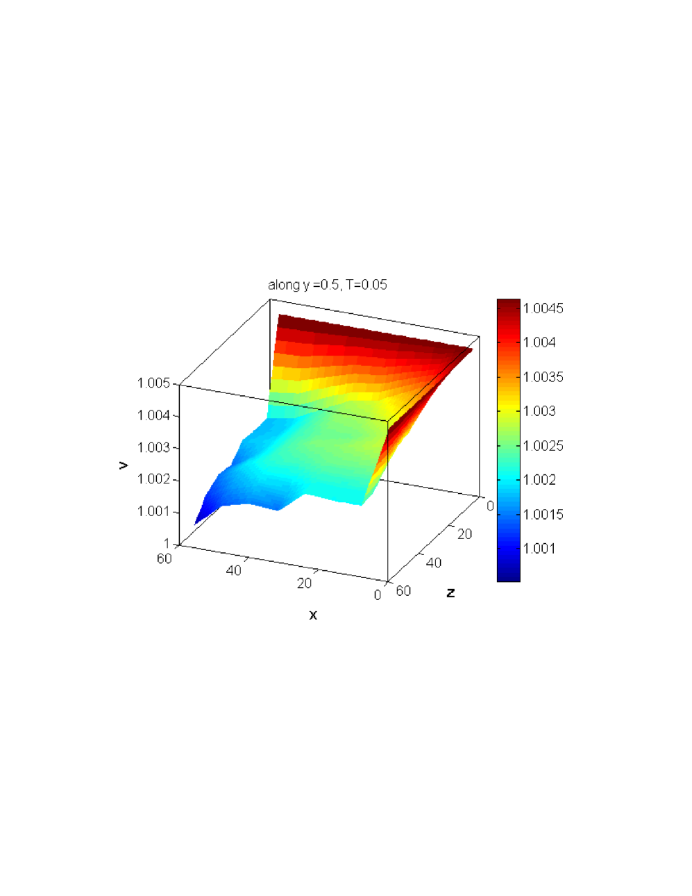
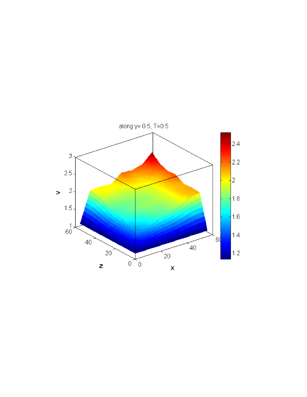
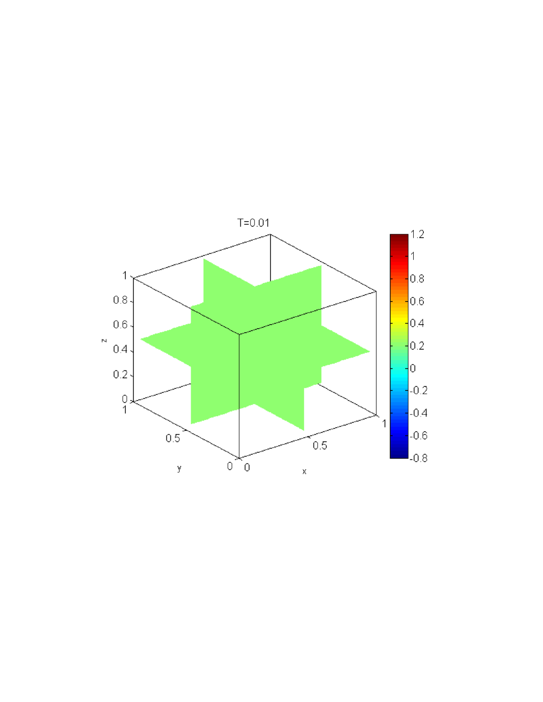
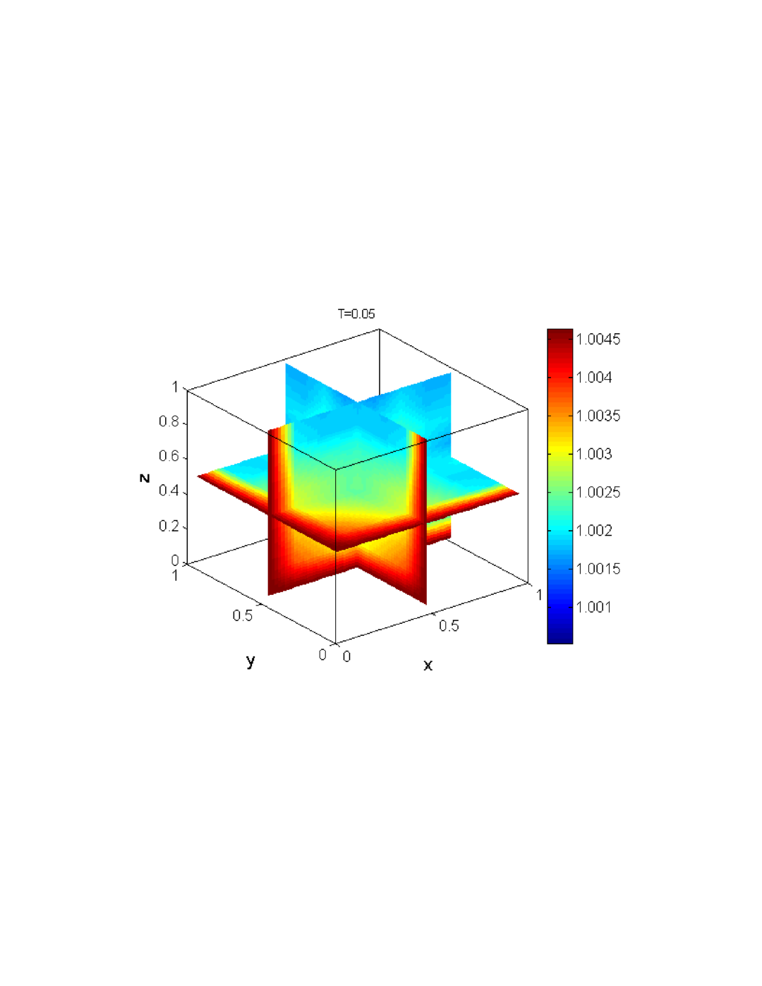
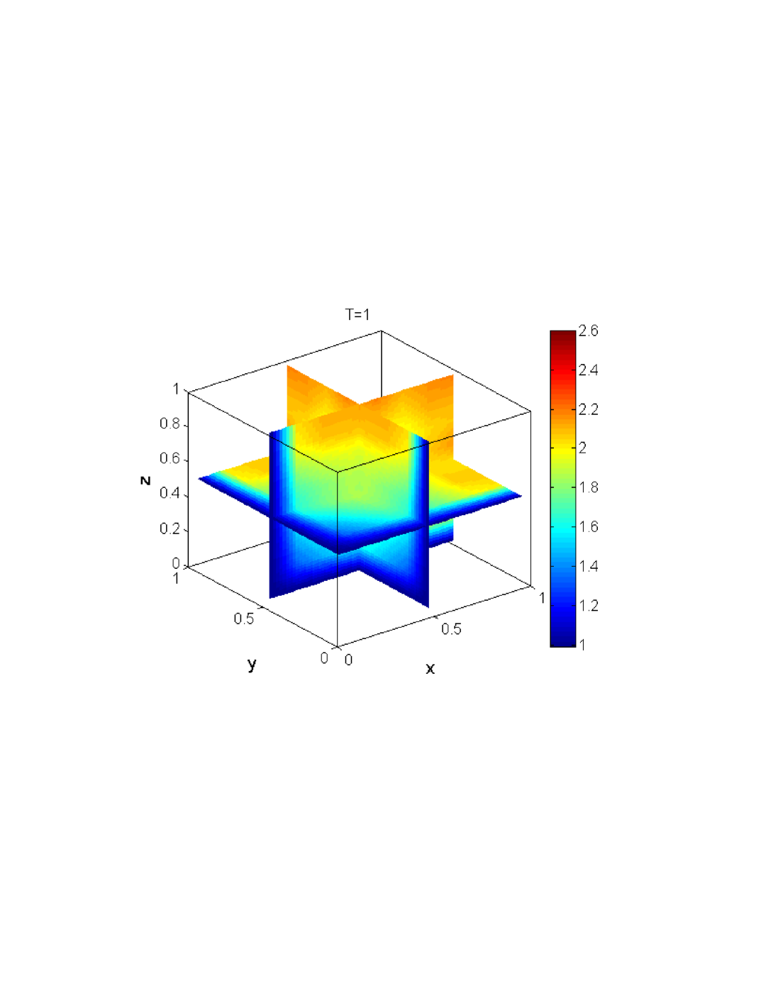
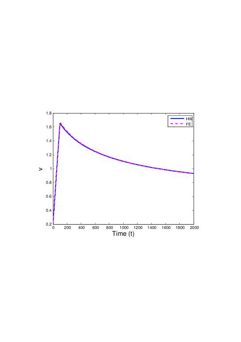
Comparison of the solution of this system using Haar wavelet method and FEM is presented in Fig. 21. We have drawn the solution along the three cross section in the 3-dimensional domain in figures (22), (23) and (24) respectively at time T=0.05 and T=0.5. We have also shown the solution v𝑣v in 3-dimensional slice at different time levels in Fig 25.
Refer to caption
Figure 21: Comparison FE and HW solution v𝑣v with J=4 and T=1 and dt=103𝑑𝑡superscript103dt=10^{-3}. at point (0.5312, 0.5312, 0.5312).
Refer to caption
(a)
Refer to caption
(b)
Refer to caption
(c)
Figure 22: HW solution along z=0.5 at time, (a) T=0.05, (b) T=0.05 (rotate view) (c)T=0.5.
Refer to caption
(a)
Refer to caption
(b)
Refer to caption
(c)
Figure 23: HW solution along x=0.5 at time, (a) T=0.05, (b) T=0.05 (rotate view) (c)T=0.5
Refer to caption
(a)
Refer to caption
(b)
Refer to caption
(c)
Figure 24: HW solution along y=0.5 at time, (a) T=0.05, (b) T=0.05 (rotate view) (c)T=0.5.
Refer to caption
(a)
Refer to caption
(b)
Refer to caption
(c)
Refer to caption
(d)
Figure 25: HW solution in the Three dimensional domain at J=4, dt=102𝑑𝑡superscript102dt=10^{-2} at time, (a) T=0.01, (b) T=0.05,(c) T=0.1, (d) T=1.

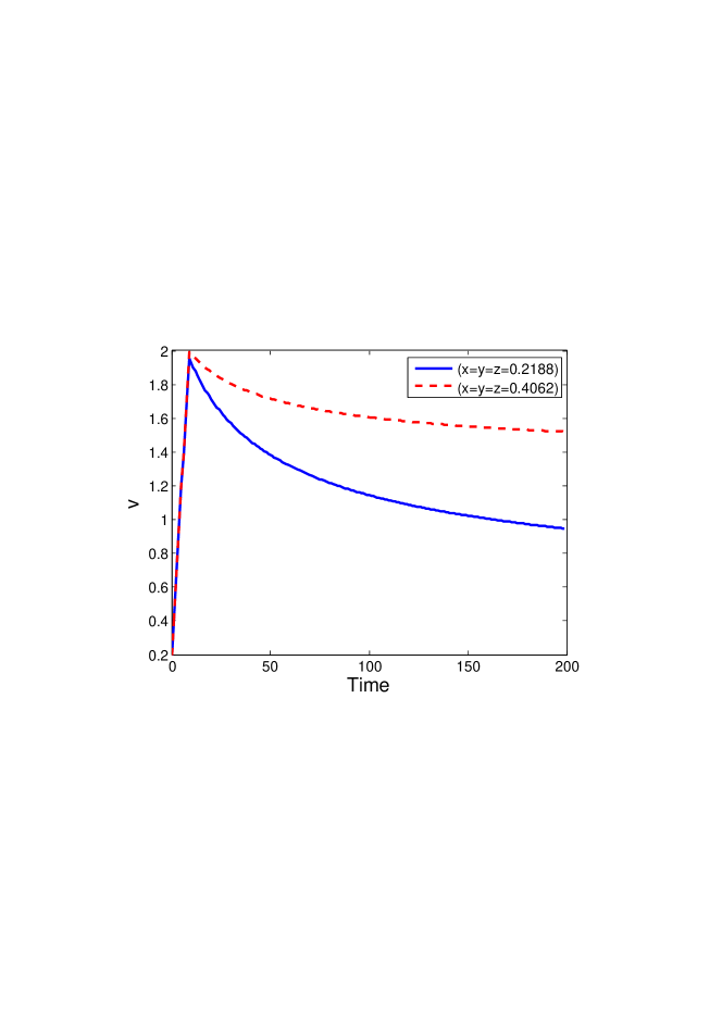
Next, we calculate the solution of the problem if the parameter τinsubscript𝜏𝑖𝑛\tau_{in} have jump discontinuity at some places in the domain, the corresponding function Iion(v,w)subscript𝐼𝑖𝑜𝑛𝑣𝑤I_{ion}(v,w) will also be discontinuous, as shown in two dimensional case. The solution v𝑣v corresponding to this τinsubscript𝜏𝑖𝑛\tau_{in} at the points (0.4062, 0.4062, 0.4062) and (0.2188, 0.2188, 0.2188), which are presented inside and outside the jump region respectively, of the domain is shown in Fig. 26. The smoothness of the solution with jump clearly shows that the Haar wavelets handle the jump discontinuity in the value of parameter τinsubscript𝜏𝑖𝑛\tau_{in}.

Refer to caption
Figure 26: Solution v𝑣v with τinsubscript𝜏𝑖𝑛\tau_{in} parameter value having jump discontinuity.

We also solved this problem using the linear finite element in space and implicit-explicit (IE) Euler method in time. Comparison of the computation time of finite element solution and the Haar wavelet solution for 3D level model in example 5 is given in Table 4. Clearly, from the table, the Haar wavelet method reduces the computational cost in comparison of FEM. Thus, it could be concluded that in higher dimension it is easy to use the Haar wavelet method to solve any problem even having the discontinuities.

J dt FEM CPU time (sec) HW CPU time (sec)
Example 5 2 (256 grid) 102superscript10210^{-2} 73.7888 40.9545
3 (1024 grid) 102superscript10210^{-2} 571.902 143.249
Table 4: CPU time in 3D
J cgs bicg bicgstab gmres
J=5,dt=103formulae-sequence𝐽5𝑑𝑡superscript103J=5,dt=10^{-3}(1D model) 7.629 6.70 8.345 5.2011
J=4,dt=103formulae-sequence𝐽4𝑑𝑡superscript103J=4,dt=10^{-3}(2D model) 6.9015 6.8364 7.07158 6.4849
J=3,dt=102formulae-sequence𝐽3𝑑𝑡superscript102J=3,dt=10^{-2}(3D model) 85.14 81.1456 83.8982 72.875
Table 5: CPU time with different solvers for 1D, 2D, and, 3D problems

6 Conclusion

A Haar Wavelet Method for a class of coupled non-linear PDE-ODEs system with jump discontinuities in model parameters or model coefficients has been proposed. The method is both simple and easy to implement in two and three dimensions. It is also computationally cost effective over linear finite element method. ILU- preconditioned GMRES Krylov solver accelerates the numerical solution convergence of the related linear system to required tolerances faster than other regular Krylov solvers. Convergence analysis has also been done to ensure the stability and accuracy. Numerical error reduces with the decrease in time step size or increase in resolution level. Model problems having single or multiple jump discontinuities in some parameters have been successfully solved. Behavior of the solutions clearly indicated that Haar wavelets automatically handle such type of discontinuities. Problems with clinical relevance have also been successfully dealt with.

Acknowledgements.
Authors would to acknowledge SERB. Govt of India for funding the project (SERB/F/10196/2017-2018) on WGM for PDEs. We would also like to thank the DST for support through Inspire Fellowship, ID no. is IF130906.

References

  • Aziz and Fayyaz (2013) Aziz I, Fayyaz M (2013) A new approach for numerical solution of integro-differential equations via haar wavelets. International Journal of Computer Mathematics 90(9):1971–1989
  • Aziz et al. (2010a) Aziz I, Haq F, et al. (2010a) A comparative study of numerical integration based on haar wavelets and hybrid functions. Computers & Mathematics with Applications 59(6):2026–2036
  • Aziz et al. (2010b) Aziz I, Šarler B, et al. (2010b) The numerical solution of second-order boundary-value problems by collocation method with the haar wavelets. Mathematical and Computer Modelling 52(9-10):1577–1590
  • Aziz et al. (2011) Aziz I, Khan W, et al. (2011) Quadrature rules for numerical integration based on haar wavelets and hybrid functions. Computers & Mathematics with Applications 61(9):2770–2781
  • Aziz et al. (2012) Aziz I, Khan W, et al. (2012) Numerical integration of multi-dimensional highly oscillatory, gentle oscillatory and non-oscillatory integrands based on wavelets and radial basis functions. Engineering Analysis with Boundary Elements 36(8):1284–1295
  • Aziz et al. (2013a) Aziz I, Šarler B, et al. (2013a) Wavelets collocation methods for the numerical solution of elliptic bv problems. Applied Mathematical Modelling 37(3):676–694
  • Aziz et al. (2013b) Aziz I, et al. (2013b) New algorithms for the numerical solution of nonlinear fredholm and volterra integral equations using haar wavelets. Journal of Computational and Applied Mathematics 239:333–345
  • Bernardi and Verfürth (2000) Bernardi C, Verfürth R (2000) Adaptive finite element methods for elliptic equations with non-smooth coefficients. Numerische Mathematik 85(4):579–608
  • Bonito and Devaud (2015) Bonito A, Devaud D (2015) Adaptive finite element methods for the stokes problem with discontinuous viscosity. Mathematics of Computation 84(295):2137–2162
  • Bonito et al. (2013) Bonito A, DeVore RA, Nochetto RH (2013) Adaptive finite element methods for elliptic problems with discontinuous coefficients. SIAM Journal on Numerical Analysis 51(6):3106–3134
  • Bourgault et al. (2006) Bourgault Y, Coudière Y, Pierre C (2006) Well-posedness of a parabolic problem based on a bidomain model for electrophysiological wave propagation. Preprint
  • Bujurke et al. (2008) Bujurke N, Salimath C, Shiralashetti S (2008) Numerical solution of stiff systems from nonlinear dynamics using single-term haar wavelet series. Nonlinear Dynamics 51(4):595–605
  • Chen and Hsiao (1997) Chen C, Hsiao C (1997) Haar wavelet method for solving lumped and distributed-parameter systems. IEE Proceedings-Control Theory and Applications 144(1):87–94
  • Comincioli et al. (2000) Comincioli V, Naldi G, Scapolla T (2000) A wavelet-based method for numerical solution of nonlinear evolution equations. Applied numerical mathematics 33(1-4):291–297
  • Daafouz et al. (2014) Daafouz J, Tucsnak M, Valein J (2014) Nonlinear control of a coupled pde/ode system modeling a switched power converter with a transmission line. Systems & Control Letters 70:92–99
  • Duarte and Oden (1996) Duarte CA, Oden JT (1996) An hp adaptive method using clouds. Computer methods in applied mechanics and engineering 139(1-4):237–262
  • Fries and Belytschko (2010) Fries TP, Belytschko T (2010) The extended/generalized finite element method: an overview of the method and its applications. International Journal for Numerical Methods in Engineering 84(3):253–304
  • Göktepe and Kuhl (2010) Göktepe S, Kuhl E (2010) Electromechanics of the heart: a unified approach to the strongly coupled excitation–contraction problem. Computational Mechanics 45(2-3):227–243
  • Hariharan and Kannan (2010) Hariharan G, Kannan K (2010) Haar wavelet method for solving some nonlinear parabolic equations. Journal of mathematical chemistry 48(4):1044–1061
  • Hodgkin and Huxley (1952) Hodgkin AL, Huxley AF (1952) A quantitative description of membrane current and its application to conduction and excitation in nerve. The Journal of physiology 117(4):500–544
  • Keener and Sneyd (1998) Keener J, Sneyd J (1998) Mathematical physiology, Interdisciplinary Applied Mathematics, vol 8. Springer-Verlag, New York
  • Kestler et al. (2016) Kestler S, Steih K, Urban K (2016) An efficient space-time adaptive wavelet galerkin method for time-periodic parabolic partial differential equations. Mathematics of Computation 85(299):1309–1333
  • Lepik (2007) Lepik Ü (2007) Numerical solution of evolution equations by the haar wavelet method. Applied Mathematics and Computation 185(1):695–704
  • Paolucci et al. (2014) Paolucci S, Zikoski ZJ, Grenga T (2014) Wamr: An adaptive wavelet method for the simulation of compressible reacting flow. part ii. the parallel algorithm. Journal of Computational Physics 272:842–864
  • Plonsey (1988) Plonsey R (1988) Bioelectric sources arising in excitable fibers (alza lecture). Annals of biomedical engineering 16(6):519–546
  • Šarler et al. (2011) Šarler B, Aziz I, et al. (2011) Haar wavelet collocation method for the numerical solution of boundary layer fluid flow problems. International Journal of Thermal Sciences 50(5):686–697
  • Schneider and Vasilyev (2010) Schneider K, Vasilyev OV (2010) Wavelet methods in computational fluid dynamics. Annual review of fluid mechanics 42:473–503
  • Sepulveda et al. (1989) Sepulveda NG, Roth BJ, Wikswo Jr JP (1989) Current injection into a two-dimensional anisotropic bidomain. Biophysical journal 55(5):987
  • Shi and Cao (2012) Shi Z, Cao Y (2012) Application of haar wavelet method to eigenvalue problems of high order differential equations. Applied Mathematical Modelling 36(9):4020–4026
  • Singh and Kumar (2017) Singh I, Kumar S (2017) Wavelet methods for solving three-dimensional partial differential equations. Math Sci (Springer) 11(2):145–154, DOI 10.1007/s40096-017-0220-6, URL https://doi.org/10.1007/s40096-017-0220-6
  • Vasilyev et al. (2004) Vasilyev OV, Gerya TV, Yuen DA (2004) The application of multidimensional wavelets to unveiling multi-phase diagrams and in situ physical properties of rocks. Earth and Planetary Science Letters 223(1-2):49–64
  • Veneroni (2009) Veneroni M (2009) Reaction-diffusion systems for the macroscopic bidomain model of the cardiac electric field. Nonlinear Anal Real World Appl 10(2):849–868, DOI 10.1016/j.nonrwa.2007.11.008, URL https://doi.org/10.1016/j.nonrwa.2007.11.008
  • Vynnycky and Mitchell (2013) Vynnycky M, Mitchell S (2013) On the accuracy of a finite-difference method for parabolic partial differential equations with discontinuous boundary conditions. Numerical Heat Transfer, Part B: Fundamentals 64(4):275–292
  • Wu (2009) Wu JL (2009) A wavelet operational method for solving fractional partial differential equations numerically. Applied Mathematics and Computation 214(1):31–40