Wiener densities for the Airy line ensemble
Abstract
The parabolic Airy line ensemble is a central limit object in the KPZ universality class and related areas. On any compact set , the law of the recentered ensemble has a density with respect to the law of independent Brownian motions. We show that
where S is an explicit, tractable, non-negative function of . We use this formula to show that is bounded above by a -dependent constant, give a sharp estimate on the size of the set where as , and prove a large deviation principle for . We also give density estimates that take into account the relative positions of the Airy lines, and prove sharp two-point tail bounds that are stronger than those for Brownian motion. These estimates are a key input in the classification of geodesic networks in the directed landscape [18]. The paper is essentially self-contained, requiring only tail bounds on the Airy point process and the Brownian Gibbs property as inputs.
1 Introduction
The Airy line ensemble is a stationary random sequence of functions satisfying . It was first introduced by Prähofer and Spohn [41] via a determinantal formula, see (9) below. Prähofer and Spohn showed that the top line –known as the Airy (or Airy2) process–describes the scaling limit at a fixed time for a certain one-dimensional random growth model in the KPZ (Kardar-Parisi-Zhang) universality class started from a point. The remaining lines describe the scaling limit of a richer multi-layer random growth model. Since this work, the Airy process and the Airy line ensemble have been shown to be universal limit objects in the KPZ universality class and other related branches of probability. Among other results, we now know:
-
(i)
The Airy process and the Airy line ensemble appear as one-parameter scaling limits of classical solvable random metric and random growth models in the KPZ universality class (e.g. zero temperature models including exponential/geometric/Poisson/Brownian last passage percolation and tasep, see [37, 41, 15, 19]; positive temperature models including the KPZ equation and the KPZ line ensemble, see [16, 43, 46, 47]). See [27, 42, 14, 44, 11] for background on the KPZ universality class and related areas.
-
(ii)
The richest scaling limit in the KPZ universality class–the directed landscape–can be described via a last passage problem across the Airy line ensemble, see [20]. Moreover, for last passage models, convergence to the Airy line ensemble is the only integrable input required for proving convergence to the directed landscape, see [23].
- (iii)
-
(iv)
The Airy line ensemble appears as the limit at the boundary between the frozen and liquid regions in general classes of random lozenge tilings, see [5], also [38, 25, 39, 40] for earlier convergence results and work on related models. The extended Airy kernel has also been found at the more delicate liquid-gas boundary in the two-periodic Aztec diamond [8, 9].
While the determinantal representation of the Airy line ensemble is useful for the definition, it can be difficult to work with in practice and does not give good intuition for the probabilistic structure of Airy line ensemble. It is more useful to view as a system of infinitely many non-intersecting Brownian motions (i.e. a limit of (iii) above).
This idea was made rigorous by Corwin and Hammond [15] by identifying a Brownian Gibbs property for the Airy line ensemble. To describe this property, we work with the parabolic Airy line ensemble , where . The Brownian Gibbs property states that inside any region , conditionally on all values for , the parabolic Airy line ensemble on is simply given by a sequence of independent Brownian bridges of variance from to conditioned so that the entire ensemble remains non-intersecting 111Here we say that a Brownian bridge has variance if its quadratic variation over any interval equals .
This property is extremely useful for understanding the Airy line ensemble. For example, the Brownian Gibbs property is necessary to rigorously show that the determinantal formula of Prähofer and Spohn defines a system of non-intersecting paths. The Brownian Gibbs property also implies that that recentered Airy lines are locally absolutely continuous with respect to Wiener measure of variance . This gives information about the sample paths of that is extremely difficult to access with the determinantal formula alone.
Given that recentered Airy lines are locally absolutely continuous with respect to Wiener measure, the next natural question is to ask exactly how this occurs. More precisely, we would like to explicitly describe the density (i.e. the Radon-Nikodym derivative) of Airy lines against Wiener measure. This is the goal of the present paper.
To state our main result, for and , let denote the space of -tuples of continuous functions with , equipped with the topology of uniform convergence. Let be the law on of
| (1) |
and let be the law on of a -tuple of independent Brownian motions of variance . In (1) and throughout the paper we write . Let be the density of against .
Theorem 1.1.
Fix . Then there exists a function such that for -a.e. we have
| (2) |
In Theorem 1.1 and throughout the paper, we write for a term that is bounded in absolute value by times a -dependent constant.
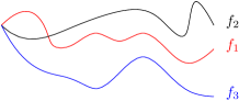
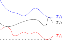
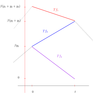
The function S is given as follows. Let denote the space of -tuples of continuous functions from with the topology of uniform convergence (without a condition on ). For , let be the minimal -tuple of functions such that
for all and such that . Here and throughout we write , etc. We think of as the “Tetris of ”: the result of consecutively dropping the graphs of the functions onto a flat line, and letting them stack up on top of each other as in the game of Tetris, see Figure 1. Then
Remark 1.2 (-dependence in Theorem 1.1).
We impose the restriction that throughout the paper in order to simplify our expression of the error term. Naturally, Theorem 1.1 immediately implies that similar bounds hold for by pushing forward the measures from to under the projection . Note that (2) also implies estimates on intervals of the form by the stationarity of .
The factor in the error is optimal as . Because of the stationarity of the Airy line ensemble the law concentrates around functions that are relatively close to the parabola . On the other hand, the probability that a Brownian motion follows this parabola up to time is easily checked to be .
1.1 More motivation and applications
The Brownian Gibbs property and the local Brownian structure of the Airy line ensemble have been repeatedly exploited to prove results about the Airy process, the Airy line ensemble, and more general limit objects in the KPZ universality class, e.g. see [15, 34] for some early examples and [30] for a survey with more recent applications. In particular, the construction of the directed landscape [20] relies heavily on Brownian Gibbs analysis from [22].
While it is quite useful to know that the Airy line ensemble is locally absolutely continuous with respect to Brownian motion, there are many situations when a more quantitative comparison is required. The search for a strong quantitative comparison was first undertaken by Hammond [35] and then continued by Calvert, Hegde, and Hammond [12]. The culmination of these two papers is the following estimate from [12]. For any , , and any Borel set we have
| (3) |
where is a -dependent constant and is Wiener measure of variance on .
While (3) looks like a fairly technical statement, it has proven to be extremely useful. Indeed, since the growth in the right-hand side of (3) is slower than any power of , it shows that events for Brownian motion that occur with probability occur only with probability for the th Airy line. This is a key estimate for ruling out pathological behaviour in the Airy line ensemble, and has been used repeatedly for understanding limiting random geometry in the KPZ universality class, e.g. see [7, 28, 32, 6, 34, 36, 33, 29, 10, 24, 21].
Theorem 1.1 strengthens the estimate (3). In fact, it implies something more surprising: namely, that the left-hand side of (3) is uniformly bounded over all !
Corollary 1.3.
For every , we have that for -a.e. . In other words, for any Borel set .
It is worth noting that our proof of Theorem 1.1 and Corollary 1.3 is shorter than the proof of (3) from [35, 12], and hence gives an easier route to this cornerstone result and its consequences.
Corollary 1.3 bounds how large can be compared to . We can also use Theorem 1.1 to get a sharp estimate on how small can be compared to .
Corollary 1.4.
Define the function by
and let be the maximum of on the sphere . Then
| (4) |
Note that the decay on the right-hand side of (4) is slower than any power of . Because of this, we expect that Corollary 1.4 could be useful for showing that rare behaviour for Brownian motion also occurs in the Airy line ensemble and the directed landscape, just as (3) has been used previously for ruling out certain behaviour in these objects.
For general , the minimum value of does not have a nice closed form. However, when , then the minimum value is (i.e. when ). The proof of Corollary 1.4 also gives a sense of what types of sets will come close to achieving the infimum in (4).
Remark 1.5.
As another application, we can quickly deduce a large deviation principle for by using Corollaries 1.3 and 1.4 and Schilder’s theorem. Note that this does not require the full strength of the above results, only that for all .
Corollary 1.6.
For every , let denote the pushforward on of under the map . Also, for , define the rate function
if is absolutely continuous, and otherwise. Then for every open set we have
and for every closed set we have
1.2 A tool for Airy analysis
While the Brownian Gibbs property is a powerful tool for analyzing the Airy line ensemble, it can nonetheless be difficult to analyze a collection of non-intersecting Brownian bridges on conditioned to stay above a possibly arbitrary and unknown boundary. Indeed, at this point there is a fairly substantial bag of tricks designed precisely to handle these issues (e.g. monotonicity ideas [15], the bridge representation [22], the Wiener candidate and jump ensemble methods [35, 12], tangent methods [31]).
One of the main contributions of this paper is to construct a line ensemble that is equal to the Airy line ensemble under a certain non-intersection conditioning, but is given by independent Brownian bridges on the region . The existence of the line ensemble implies Wiener density bounds that are similar to (3) and (1.3), but crucially take into account the locations of the Airy endpoints.
As our main theorem about the line ensemble has a somewhat technical statement, we first give an example of its use that only concerns a single Airy line.
Example 1.7.
Fix . Then the law of process has a bounded density against the law of a process , where:
-
•
is a Brownian bridge of variance with .
-
•
is an affine function, independent of , and there are -dependent constants such that for all we have
(5) (6)
The one-point bounds on in Example 1.7 give the same stretched exponential tail behaviour as for the Tracy-Widom random variable . Moreover, the two-point bound on is actually stronger than the same bound for a variance Brownian motion! We now state the main theorem about the line ensemble .
Theorem 1.8.
Fix . Then there exists a random sequence of continuous functions such that the following points hold:
-
1.
Almost surely, satisfies for all pairs .
-
2.
The ensemble has the following Gibbs property. For any set , conditional on the values of for , the distribution of is given by independent Brownian bridges from to for , conditioned on the event whenever .
In particular, the law of on is simply given by independent Brownian bridges connecting to .
-
3.
We have
and conditional on the event , the ensemble is equal in law to the parabolic Airy line ensemble .
The process in Example 1.7 is given by . The strong one- and two-point tail bounds in that example follow from more general tail bounds on proven in Sections 4 and 5. These tail bounds make the line ensemble useful for analysis in practice.
Remark 1.9.
Remark 1.10.
Theorem 1.8 allows us to relax the Brownian Gibbs property for by removing the non-intersection condition on the patch . We can also give a more general version of Theorem 1.8 that removes the non-intersection condition on disjoint patches for a vector . If we call the new line ensemble , then ; crucially, this bound does not depend on . Moreover, the patches become asymptotically independent as . The line ensembles are useful for studying the Airy process and the Airy line ensemble on large spatial scales. See Theorem 3.8 for details.
1.3 A heuristic for (2): Brownian motion avoiding a parabola
Before giving a brief overview of the proof in Section 1.4, we a heuristic for formula (2). For simplicity, we will only consider the case when . A good starting point for trying to understand the behaviour of the top curve is the well-known pair of tail estimates
| (7) |
Similar estimates hold for all Airy lines, see Lemmas 2.1, 2.2. The intuition from these estimates suggests first that typically adheres to the parabola , and secondly that it is much easier for to move up away from this parabola than it is for to push down below the parabola. Because of this, a toy model for can be given as follows. Consider a sequence of Brownian bridges from to conditioned to stay above the parabola , and take to to get a distributional limit . The process has been studied in [26] and can actually be described as a diffusion with an explicit drift involving Airy functions. However, for this discussion we will stick to softer intuition regarding .
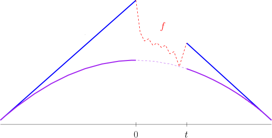
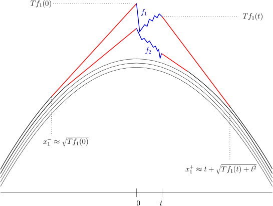
One way to check the reasonability of this toy model is to check the probability that . The best way for to equal should be if only deviates from the parabola by following straight lines from to and back to for some . Computing the Dirichlet energy of this path against the Dirichlet energy of the parabola, and optimizing over yields that our best guess for should be , which agrees with the Tracy-Widom upper tail on . The optimal value is ; with this choice the straight lines from and to are tangent to the parabola.
Next, for to equal a function , we must have for all . From the definition of the tetris map T, we can observe that
Since it is costlier to raise up further away from the parabola, this implies that the optimal way to have equal to is to let sit in the interval and similarly let sit in the interval . The cost of this, relative to the cost of simply having a Brownian motion equal to can again be computed by comparing the Dirichlet energy of straight lines against a parabola. Assuming is very small relative to the size of , this amounts to computing the Dirichlet energy of the straight line from to plus the Dirichlet energy of the straight line from to minus the Dirichlet energy of the parabola from to . This is
which is . See Figure 2 for an illustration. The intuition behind the expression (2) for more than one line is similar, except now we need to stack the functions on top of each other, and on top of the parabola in order to achieve the ordering .
Understanding probabilistic objects built from non-crossing paths via a tangent picture is not a new idea. Indeed, tangent methods were proposed by Colomo and Sportiello [13] for studying limit shapes of the six-vertex model, and made rigorous by Aggarwal [4]. In the context of the KPZ and Airy line ensembles, tangent methods were used by Ganguly and Hegde [31] to pinpoint the upper tail one-point asymptotics in (7) and related upper tail two-point asymptotics using only minimal assumptions.
1.4 Outline of the proof and the paper
A priori, it is not clear why the hydrodynamic tangent heuristic should give fine control over the Wiener density. As a result, our proof of the upper bound in Theorem 1.1 does not proceed by directly trying to prove this heuristic. Rather, we first prove Theorem 1.8, which implies that the only contribution to the Wiener density comes from the joint distribution of the endpoints (here is as in Theorem 1.8). To prove Theorem 1.8, by the Brownian Gibbs property we can abstractly define a -finite measure on the space of sequences of continuous functions such that if were finite, then after scaling it to a probability measure, it would give the law of a line ensemble satisfying Theorem 1.8. The key difficulty is in showing that : here we use a refinement of some ideas from [22] and [35], along with new insights about how the Brownian Gibbs property on different domains controls . The proof of Theorem 1.8 is contained in Section 3.
In Section 4, we analyze the joint distribution of by again appealing to one-point bounds, using monotonicity arguments, and applying an induction argument to pass from control of for any fixed to joint control of . It is only because the upper tail one-point bound in (7) sharply matches the bound coming from the tangent heuristic that the tangent picture emerges. In Section 5, we combine these tail bounds with Theorem 1.8 to establish that LHSRHS in (2).
The lower bound LHSRHS is easier, since we only need to work on a part of the probability space where the st line does not deviate too far from the parabola. It closely resembles a rigorous version of the heuristic discussed in Section 1.3, and is shown in Section 6. A final section (Section 7) proves the corollaries.
We have striven to keep the paper self-contained, relying only on standard tail bounds on the Airy points , the Brownian Gibbs property, and basic monotonicity properties for non-intersecting Brownian bridges as inputs.
Conventions throughout the paper
In all sections of the paper after Section 2, and are fixed. We will often suppress dependence of objects on and for notational convenience (e.g. we write instead of ). We write for large constants and for small constants. Our constants may change from line to line within proofs and we use a subscript (i.e. ) if they depend on . Constants will not depend on any other parameters. All Brownian objects in the paper (e.g. Brownian bridge, Wiener measure) will have variance , as is the convention for the Airy line ensemble. For a set , we write (respectively ) for all with (respectively ). For a sequence of functions and , we write for the first coordinates of . Finally, we use the shorthand for conditional expectation with respect to a -algebra .
2 Preliminaries
In this section, we introduce a few basic preliminaries about the Airy line ensemble and other non-intersecting collections of Brownian motions.
Let be a closed interval in , let , and define denote the space of -tuples of continuous functions from to with the compact topology
We also let be the space of all sequences of continuous functions from to , again equipped the with compact topology (we replace with in the definition above), and we write .
We can also think of as a function with the topology of uniform convergence on compact subsets of , and with this in mind, we will often write for the restriction of to a subset of . For with we write for the first coordinates of .
The parabolic Airy line ensemble is a random element of (a.k.a. a line ensemble) satisfying
almost surely. The process is the usual Airy line ensemble and is stationary under shifts and flips. For any we have
| (8) |
where the equality in distribution is as random element of . Throughout the paper we will typically use the parabolic version , which has a more natural Gibbs resampling property. The Airy line ensemble is uniquely characterized by a determinantal formula. Indeed, for every finite set of times , the set of locations set is a determinantal point process on with with kernel
| (9) |
where is the Airy function.
2.1 Tail bounds
The Airy points satisfy well-known tail bounds. A fairly sharp upper tail bound is a quick consequence of the determinantal formula.
Lemma 2.1.
For all there exists such that for we have
Proof.
This is a simple calculation involving the Airy kernel at a single time. Let Then for and we have
As long as is small enough, the right hand side above equals
where is the Airy kernel. Taking , we see that has a Lebesgue density that at is bounded above by
Using the formula (9) and the standard bound for a universal constant (see formula 10.4.59 in [2]), we have that
and so
Integrating this over the set of all with for all yields the result. ∎
Lemma 2.2.
For every there exists such that for all we have
| (10) |
Proof.
Later on in the paper, we will need a quick way to move between two-point tail bounds and a maximum bound on a stochastic process. This is accomplished through the following lemma.
Lemma 2.3.
Let , and suppose that there exist constants such that for all and all , we have the estimate
Then for we have
Proof of Lemma 2.3.
The proof is a standard chaining argument. We may assume , and focus on bounding . For every , let be the function with for for some , and such that is linear on each of the intervals . For , let , where . We can write . Also,
and hence we have the union bound
Therefore letting
we have Next,
which yields the result after converting the tail bound on . ∎
2.2 Gibbs resampling
As discussed in the introduction, the Airy line ensemble satisfies a resampling property called the Brownian Gibbs property. Here we make introduce notation that will help us work with the Brownian Gibbs property, and state a few useful lemmas.
First, for an interval , an interval and an -valued function whose domain contains , let
Note that the value of and the interval is not explicit in the notation . These will always be clear from context (i.e. by specifying the initial space ). We will use the shorthand . Next, we say that a -tuple of independent Brownian bridges goes from to for if each of the is a Brownian bridge with . Note that our bridges will always have variance . We write
for the probability that a -tuple of independent Brownian bridges from to is in the non-intersection set . Again, we omit from all notation if . We say that the -tuple of Brownian bridges is non-intersecting if it is conditioned on the event .
The Brownian Gibbs property for can now be more formally stated as follows:
-
For a set , let denote the -algebra generated by . Then the conditional distribution of given is equal to the law of independent Brownian bridges from to conditioned on the event .
In the statement above, recall that and note that when applying the Gibbs property, the bridges are always drawn independently of the endpoint vectors and of the lower boundary .
We record two key lemmas that will allow us to work with the Brownian Gibbs property. The first is a crucial monotonicity property.
Lemma 2.4.
Let be closed intervals in with , let where is the coordinate-wise partial order, and let be bounded Borel measurable functions from . For be be a -tuple of Brownian bridges from to , conditioned on the event . Then there exists a coupling such that for all .
Lemma 2.4 is proven as Lemmas 2.6 and 2.7 in [15] in the case when . The proof goes through verbatim in the slight extension when is a strict subset of .
The next lemma is a lower bound on the probability of Brownian bridges being non-intersecting. This bound will allow us to compare regular Brownian bridge probabilities with non-intersecting bridge probabilities.
Lemma 2.5.
Let be vectors with
for some . Let . Then setting we have
This lemma is fairly standard and follows from the Karlin-McGregor formula. For example, it is very similar to Proposition 3.1.1 in [35], and we follow the same steps used in the proof of that proposition.
Proof.
First, where . Therefore letting , by the Karlin-McGregor formula, after simplification we can write
See the middle of p. 48 in [35] for this version of the Karlin-McGregor formula. The determinant is a Vandermonde, and satisfies
Finally
yielding the result. ∎
3 Constructing
In this section, we construct the line ensemble and prove Theorem 1.8. Throughout the section, we fix .
Let be the parabolic Airy line ensemble. We will define a -finite measure on according to the following procedure.
-
1.
First, define a line ensemble by letting for , and let be given by independent Brownian bridges from to . These bridges are independent of each other and of . Let denote the law of .
-
2.
Let be the measure which is absolutely continuous with respect to with density given by
(11) for . This density exists for -a.e. since , , and almost surely, and .
We would like to say that is a finite measure, and hence can be normalized to a probability measure. This normalized measure will be the law of the line ensemble . Once we know this, Theorem 1.8 will follow easily. However, it is highly non-trivial to show that is finite. The bulk of this section is devoted to proving this. Indeed, by (11) we can observe that
| (12) |
and so concretely we just need to show that the inverse acceptance probability
has finite expectation. In order to do this, we will study alternate constructions of the measure . Fix , and define a measure by the following procedure:
-
1.
Define a line ensemble by letting for , and let have the conditional law given outside of of independent Brownian bridges from to conditioned on the event
Let denote the law of .
-
2.
Let be the measure which is absolutely continuous with respect to with density given by
(13) for .
Lemma 3.1.
For every , we have , and letting be the -algebra generated by the Airy line ensemble outside of the set , we have
| (14) |
Equation (14) exchanges the expectation of an inverse for the inverse of an expectation, which is much easier to bound.
The idea that the inverse acceptance probability can be controlled by an inverse of a conditional expectation by ‘stepping back’ onto the interval and applying the Brownian Gibbs property on is inspired by the Wiener candidate method of Brownian Gibbs resampling introduced by Hammond [35], see also [12].
Proof.
We first compute the density of against (more precisely, the density of against ). First, letting we have that outside of . Therefore the density of against is the same as the density of against .
Conditional on , all of and have densities with respect to the law of independent Brownian bridges from to . The density of is is given by
| (15) |
for . The density of is
| (16) |
for . We obtain from by replacing with independent Brownian bridges on from to . The density of on with respect to independent Brownian bridges between these points is given (again by the Brownian Gibbs property) by
| (17) |
for . Therefore the density of with respect to the law of independent Brownian bridges from to is simply the product of (16) with the inverse of (17) at the function . This is
| (18) |
The ratio of (18) and (15) gives the density of against , conditional on :
| (19) |
for . Using this, and the definitions (11), (13) of from gives that . For the equality (14), using that the first factor in (19) is -measurable, we have that
which equals . ∎
The goal of the next few lemmas is to estimate the right-hand side of (14). The first lemma gives a bound on the right-hand side of (14) in terms of a few simple -measurable random variables.
Lemma 3.2.
Fix and define -measurable random variables
Then with as in the previous lemma, we have
We separate out one of the main calculations for Lemma 3.2, as it will also be required later in the paper.
Lemma 3.3.
Let , and . Let be such that .
Let be a -tuple on independent Brownian bridges from to , conditioned on the event
Define , and for define by letting
and so that is linear on each of the pieces .
Then for we have that
| (20) |
The more formal way to interpret (20) is as a bound on the density of the law of against the law of , on the set where is absolutely continuous with respect to .
Proof.
Let be the law of independent Brownian bridges from to . Observe that are absolutely continuous with respect to with densities
| (21) |
where is a normalizing factor. Now, if is in the set , then so is . Hence the right-hand side of (20) is bounded below by the exponential factor (21). We can bound (21) below by using that , and that , which yields the desired bound. ∎
Proof of Lemma 3.2.
All statements in the proof are conditional on . Define the -measurable vector
and the -measurable set
| (22) |
By the definition of , for we have
| (23) |
where is a Brownian bridge from to . By a standard bound, the right hand side above is bounded below by . Therefore letting denote the conditional law of given , to complete the proof it suffices to find a set such that is large. Fix and let be the -measurable subset of where
for all . Then by Lemma 3.3 with , we have
| (24) |
It remains to find where is large. Define vectors where
By Lemma 2.4, on the interval , the -tuple is stochastically dominated by independent Brownian bridges from to conditioned on the event
Now, let be the function whose th coordinate is the linear function satisfying . Observe that by the construction of , we have for any sequence of bridges from to with . The probability that this condition holds for a sequence of independent Brownian bridges is bounded below by (similarly to the bound on (23)). Therefore
Observing that
for all , we can conclude that
Combining this with the bound on (23) and (24) and simplifying yields the result. ∎
It remains to prove tails bounds on . The key is a two-point estimate for the Airy line ensemble. In Section 4.2 will prove a highly refined two-point estimate directly for , whose proof goes through verbatim for . However, the full power of such an estimate is not necessary and we make do with the following lemma, whose proof is much less involved.
Lemma 3.4.
For every there exists such that for all we have
| (25) |
The proof for Lemma 3.4 is similar to the proof of Lemma 6.1 in [22], except here we keep closer track of the error terms. Somewhat remarkably, this already gives a stronger tail bound than for Brownian motion when is large enough. We will need the more nuanced method in Section 4.2 to give a stronger tail bound than Brownian motion for all .
Proof.
By stationarity, it suffices to prove the lemma when . Moreover, since , it suffices to prove the bound with the absolute value removed. For , define
Let be a parameter that we will optimize over. Let be the -algebra generated by outside of the set . Let , and let be a -tuple of non-intersecting Brownian bridges from to . By Lemma 2.4, given , the Airy lines stochastically dominate , so
Now let be a collection of -tuple of independent Brownian bridges from to without a non-intersection condition. By Lemma 2.5 with ,
| (26) |
Given , the increment is normal with variance and mean .
Therefore we have
| (27) |
In the final inequality, we have used that . Now, by Lemmas 2.1 and 2.2, there exists such that for all ,
Therefore is stochastically dominated by a random variable with Lebesgue density bounded above by and so
For any , if and is the argmax of , then
Using this inequality and simplifying the result gives that and so the expectation of (27) is bounded above by
| (28) |
A quick inspection reveals that the minimum value of (28) is taken when . Plugging in (which is bounded below by since ) and simplifying gives that (28) is bounded above by
Combining this with (26) yields the result. ∎
We can deduce tail bounds on and immediately from Lemma 3.4.
Lemma 3.5.
For every , there exists such that the following bounds hold for all . Letting and we have
Proof.
We can finally give a concrete bound on , which in turn shows that the measure is finite.
Corollary 3.6.
There exists such that for all we have
| (29) |
with probability at most . In particular, .
Proof.
Let . Without loss of generality, we may assume for some large constant , since otherwise the bound holds trivially. Next, let Let and write . Then by Lemma 3.5, for and we have Moreover, by Lemma 3.2, we have
Therefore the probability of the event (29) is at most
where we have used the lower bound on and the tail bound on to achieve the bound. ∎
By Corollary 3.6, is a finite measure, and so the normalized measure is a probability measure. Let denote a line ensemble whose law is equal to . It is easy to check that satisfies Theorem 1.8.
Proof of Theorem 1.8.
Part is immediate from the definition of . Next, by the definition (11), restricting to the set
gives a probability measure. By the Brownian Gibbs property, this measure is the law of . Therefore conditioning to lie in gives a parabolic Airy line ensemble. The bound follows from the bound on in Corollary 3.6. This gives Theorem 1.8.3.
For part , first observe that if satisfies the desired Gibbs property on all sets where and , then it satisfies the Gibbs property everywhere. Fix such a set . Recalling the definition of from the construction of , and let be coupled to as in that construction. We first compute the conditional density of against the law of independent Brownian bridges from to . Let and . First, so by the Brownian Gibbs property for we have
| (30) |
where in the indicator above we say that , and is the -measurable normalization factor . Next, given , the distribution of is that of independent Brownian bridges from to . As the same is true of the unconditioned bridges , the density
is the same as the right-hand side of (30). Therefore by (11), if consists of independent Brownian bridges from to then
where is a new - measurable normalization factor. This is the desired Gibbs property. ∎
Remark 3.7.
It is interesting to note that Theorem 1.8 already implies that on the set , if is the function whose coordinates are linear functions given by the conditions , then has a uniformly bounded density against the law of independent Brownian bridges.
3.1 The line ensembles
Next, we construct the more general line ensembles introduced in Remark 1.10.
Theorem 3.8.
Fix and such that for all . Define .
Then there exists a random sequence of continuous functions such that the following points hold:
-
1.
Almost surely, satisfies for all pairs .
-
2.
The ensemble has the following Gibbs property. Let and and set . Then conditional on the values of for , the distribution of is given by independent Brownian bridges from to for , conditioned on the event whenever .
-
3.
We have
(31) and conditional on the event , the ensemble is equal in law to the parabolic Airy line ensemble .
Proof.
First, by shift invariance of we may assume . In this case, we can construct by taking the line ensemble from Theorem 1.8 and conditioning on the avoidance event
This line ensemble satisfies properties above by virtue of the same properties for . It remains to obtain the lower bound required for property .
Define a line ensemble by letting for , and for every , let be given by independent Brownian bridges from to . These bridges are independent of each other and of . Let denote the law of , and let denote the law of .
The relationship between the measures introduced here is almost the same as the relationship between the measures introduced prior to Lemma 3.1, except that here we have already normalized to a probability measure. Indeed, is absolutely continuous with respect to with density given by
where
is the expected value of a product of inverse acceptance probabilities. The probability on the left-hand side of (31) equals , so to complete the proof it suffices to show that . Indeed, we have the chain of inequalities
In the above chain the first inequality is Hölder’s inequality, the equality uses the stationarity of the Airy line ensemble, and the final inequality uses Corollary 3.6 with . ∎
4 Tail bounds for
In this section, we prove one- and two-time tail bounds on (including the bounds in Example 1.7). For readability, we have not aimed to prove tail bounds on the more general ensembles alongside the tail bounds for , though these can be obtained with similar methods.
As in the previous section, we fix and throughout the section. These bounds will be used in Section 5 to move from Theorem 1.8 to the upper bound in Theorem 1.1.
4.1 The one-time bound
The single-time bound is easier, so we start there. The idea is to first prove tail bounds on the line ensembles introduced for Lemma 3.1, and then deduce tail bounds on through the definition (13) and the bounds in Corollary 3.6.
Lemma 4.1.
Let and define the set
Then for we have
Proof.
First, the bound is immediate from Lemma 2.1 when since when . The case when is more involved. Let
Define a line ensemble by letting for , and let have the conditional law given of independent Brownian bridges from to conditioned on the event
In words, is defined similarly to , except with the extra condition that on the interval . Then by Lemma 2.4, is stochastically dominated by , so by Lemma 2.1, we have
| (32) |
for all , . Our goal is to effectively compare to conditionally on the -algebra in order to apply this bound. By Lemma 3.3 (and with notation as in that lemma), for any we have
On the other hand, the conditional laws of and given are mutually absolutely continuous with density
In particular, if for all for some , then by Lemma 2.5, this is bounded below by Putting this together with the previous bound implies that for , setting
and , we have
| (33) |
Therefore for every and we have
Upon taking expectations of both sides, we get that
It remains to bound and then optimize over . Define vectors where
By Lemma 2.4, on the interval is stochastically dominated by independent Brownian bridges from to conditioned on the event
Now, by the construction of , the probability that independent Brownian bridges from to satisfy is bounded below by . Therefore
where is an independent Brownian bridge from to . We can bound the first of these terms with Lemma 2.1, Lemma 2.2, and Lemma 3.5. The second of these terms can be bounded with a standard Brownian bridge bound. Altogether, we get that both of terms are of size as long as . Therefore setting and applying the bound (32), we get
which gives the desired result. ∎
We can translate Lemma 4.1 into a one-time bound on .
Lemma 4.2.
For any and we have
Proof.
First, we may assume since otherwise the bound is trivial. We use the notation introduced prior to Lemma 3.1. For every , we have that
Now, the density can be thought of as an -valued random variable whose domain is the Borel space with probability measure . When thought of this way, it is equal in distribution to
By the tail bounds in Corollary 3.6 on this random variable, for we then have
Therefore by Lemma 4.1, we have that
We can now minimize over . This occurs roughly when (which is greater than by our assumption), which gives the desired bound after simplification. ∎
4.2 The two-time bound
The proof of a sharp two-time bound is a much more refined version of the argument used Lemma 3.4 that takes into account the parabola. The argument is also applied to the ensemble rather than directly to . The first step is to achieve a lower bound on the probability that is small. This is achieved via the following lemma.
Lemma 4.3.
Let . Then the law of is absolutely continuous with respect to the law of and for any Borel set with have
Proof.
First, we may assume for a large constant , since otherwise the bound is trivial. Letting for some we have . Moreover, as in the proof of Lemma 4.2 we have
and minimizing at (which is greater than by our lower bound on ), gives the result. ∎
Corollary 4.4.
Fix an interval for . Then for we have
Proof.
One of the main technical ingredients we need to achieve a two-point bound is a probability estimate for a Brownian bridge avoiding a parabola.
Lemma 4.5.
Fix , and for with , define
Next let , and let . Then we have the following bounds.
-
1.
For , any with , and any , we have
-
2.
Let with , and let . If is a Brownian bridge from to , then
-
3.
Let with and for all , and suppose that . Then
The proof of Lemma 4.5 is essentially a standard Dirichlet energy computation. We sketch the idea here, and leave the details to the appendix.
First, we can set , as Brownian bridge law commutes with affine shifts. This simplifies the computations. Next, the cost for a Brownian bridge from to to roughly follow a path with is the exponentiated Dirichlet energy
This follows, for example, from the Cameron-Martin theorem. The factor of here (as opposed to the usual ) is due to the fact that we are working with variance bridges, and the added factor of comes from conditioning a Brownian motion to end at the point to give rise to a Brownian bridge. Hence we should look for a path of minimal Dirichlet energy that stays above the function . This is the minimal concave function from to that dominates . Since is just a parabola, the function is easily computed, and is determined by the following constraints:
-
•
, and there are values such that is linear on the intervals and .
-
•
for all .
-
•
is differentiable at and . This follows from forcing to be both concave and to dominate .
We can compute that , and that . This gives rise to the bound in Lemma 4.5.1, and the bound in part ; the cost of having the bridges stay ordered is a lower order term. The bound in part follows similarly to part , by computing the path of minimal Dirichlet energy from to that dips below at time .
We can now state the first version of the two-time bound for .
Proposition 4.6.
Let , let and let . Define to be the unique vector with for all . Next, define
Then
| (34) |
where
The proof of Proposition 4.6 is the most technical proof in the paper, and it is based on a backwards induction on . The next lemma gives the key inductive step.
Lemma 4.7.
In the setup of Proposition 4.6, for define the sets
and for define
Note that with these definitions, and are the whole space. Then for all and we have
| (35) |
Proof.
The proof is based on a downwards induction on . In the base case when , since is the whole space, the bound is equivalent to the claim that
for . This follows from Lemma 4.2. Now assume , and that the lemma holds for for any choice of . Without loss of generality, we assume that ; the case when follows from the distributional equality
as functions in . This equality follows from the same result for . There are two cases here, depending on whether or . We start with the simpler case when .
Step 1: Setting up a Gibbs resampling. Let be a large -dependent constant and set
How large we need to take will be made clear in the proof. Let denote the -algebra generated by outside of the set . The basic idea of the induction is a Gibbs resampling on the set . To see how the structure will work, observe that
The set is -measurable, so for any set we have
| (36) |
Now, for every , let
and let so that . We can write
Taking expectations in (36) and applying the inductive hypothesis we get
Concretely then, to complete the proof it is enough to find a set such that is bounded above by the right-hand side of (35) and
| (37) |
Step 2: Defining and comparing to a simpler ensemble. Let be the set where:
-
•
For all , we have
-
•
We have the inequalities
and set (in the final step of the proof we will also use the set ). By Lemma 4.2, Corollary 4.4 and a union bound, as long as the constant is large enough we have that
| (38) |
which is bounded above by the right-hand side of (35) for large enough.
Now let , and let be a -tuple of independent Brownian bridges from to . Let be given by , and let denote conditioned on the non-intersection event .
By Lemma 2.4 and the Gibbs property for on the set , on the event the bottom line stochastically dominates . Therefore on :
Now,
| (39) |
and we can bound the numerator above and denominator below on the event using Lemma 4.5.
Step 3: Bounding (39). Starting with the denominator in (39), we have that
where . Moreover, on we have that
as long as was chosen large enough. Similarly,
Therefore we are in the setting of Lemma 4.5.3, and so
Turning to the numerator, we have that
The product of terms above can be bounded above by Lemma 4.5.1. Note that by the definition of as long as is large enough. The remaining -term can be bounded using Lemma 4.5.2. Together we get that the right-hand side above is bounded above by
Putting together the two bounds in this section, and using that and that gives that (39) is bounded above by
| (40) |
Now, on the set , we know that and as long as was chosen large enough we have . Applying this, and simplifying the error, we get that (40) is bounded above by
which implies the desired bound in (37).
Step 4: Completing the proof when . First, with as defined in Step 2 above, by noting that satisfies the same bound as in (38), it is enough to bound
Our strategy here is to bootstrap from the previous case, by using that the Gibbs property implies that it is unlikely for the lines in to be large at time without being large at time . Let be the -algebra generated by outside of the set . Noting that the sets are -measurable for any , for any which equals on coordinates we can write
as long as almost surely on . Now, on and conditional on , by Lemma 2.4 the vector stochastically dominates an -tuple of Brownian bridges from at time to at time , conditioned not to intersect each other. The probability of non-intersection is bounded below by by Lemma 2.5, so for any for which This holds with . Therefore
which satisfies the same upper bound as , up to a term that gets folded into the error. ∎
Proposition 4.6 implies the following simpler two-point bound, of which inequality (6) is a special case.
Corollary 4.8.
Let with and let . Let be the unique vector with for all . Next, let be the unique -tuple of linear functions satisfying , and recall the definition of the map S introduced for Theorem 1.1. Then
| (41) |
Proof.
Without loss of generality, assume . Then using the notation T for the tetris map introduced after Theorem 1.1 we have that
since the vectors are ordered. Therefore for any , with notation as in Proposition 4.6 we have
Setting , by Corollary 4.4, we have that is bounded above by the right-hand side of (41) for large enough . This uses that and that . For this choice of , the left-hand side is similarly bounded via Proposition 4.6. We have simplified the error by using that and that . ∎
5 The upper bound in Theorem 1.1
In this section we prove the upper bound in Theorem 1.1. Throughout the section we fix . For this, it is enough to prove that the upper bound holds for , since in law and only differ by a linear shift which can be wrapped into the error. Moreover, we can work with rather than , since the conditional probability that is non-intersecting––can again be wrapped into the error term in Theorem 1.1. The key step is to convert Proposition 4.6 into a density estimate.
For this lemma, we define a -finite measure on as follows. First let denote the product measure on given by Lebesgue measure on and the law of independent Brownian bridges from to on . Let denote the pushforward of under the map
where is the function which is linear in each coordinate and satisfies . Then the law of is absolutely continuous with respect to . The next lemma bounds its density.
Lemma 5.1.
Let denote the density on of against the measure . Then we have the following three bounds:
-
1.
For all we have
-
2.
For all we have
Proof.
Throughout, we work with conditional on the event , which is equal in law to . Note that this event has probability .
Bound 1: First, since given is simply given by independent Brownian bridges, the Lebesgue density of is bounded above by a constant . Moreover, has the law of independent Brownian bridges from to given . Therefore the density of against is uniformly bounded by a constant , and so is a.s. by .
Note that this density bound also holds a.s. if we condition on any information about outside of . In particular, if we let be the conditional density of against on the event and the conditional density on we have
If , then by the ordering of the lines in . Moreover, by Corollary 4.4 for , which yields the desired bound when .
Bound 2: Let be the Lebesgue density of . It is enough to prove the second bound with replaced by , since the cost of conditioning to be non-intersecting folds into the error, and has the law of independent Brownian bridges from to given .
For , let be the conditional Lebesgue density of at on the event
Since is simply a -tuple of Brownian bridges from to , we have that is bounded above by
The final error term comes from the fact that , and . Next, from Proposition 4.6, we have the bound
and by Corollary 4.4 we have for . Therefore for , we have
| (42) |
where
and
We set so that
| (43) |
Now,
| (44) |
whenever . All but terms in the sum in (42) satisfy this bound. Therefore by (42), (43), and (44) we have
since the log factor is lower order compared with the -term in . It just remains to bound below. Indeed, the bound in the lemma will follow if we can show that for every we have
| (45) |
whenever . First, for we have
| (46) |
which is bounded below by the right-hand side of (45) for any . Next, for we always have the bound
which is bounded below by the right-hand side of (45) when . Finally, for and , we can differentiate to get
As long as was chosen large enough relative to , has all its roots in the region where , and hence the minimum value of over is taken in this interval. Finally, for and we have the estimate
which completes the proof of (45) when . ∎
We are now ready to prove the upper bound in Theorem 1.1.
Corollary 5.2.
With notation as in Theorem 1.1, for -a.e. we have that
| (47) |
Proof.
With notation as in Lemma 5.1 we can write
| (48) |
Observe that unless . Equivalently, we require
| (49) |
where . here the functional T is the Tetris map from Theorem 1.1. Next, by Lemma 5.1.2 we can see that the integrand in (48) is bounded above by
| (50) |
Also, by Lemma 5.1.1, for , the integrand is bounded above by
Together with (50), this bounds implies that the contribution to the integral from the region where either or is at most which is bounded above by the right-hand side of (47).
The size of the remaining region is , which folds in to the error, so it enough to simply maximize (50) subject to the constraint (49) on the set where or . Observe that on this set, the error term in (50) is at most so it suffices to understand the main term. As the main term is decreasing in each , the minimal value occurs at . Plugging in this value for yields
as desired. ∎
6 The lower bound in Theorem 1.1
In this section we complete the proof of Theorem 1.1. For this section and are fixed throughout and we use the notation from Theorem 1.1. The proof of the lower bound for Theorem 1.1 involves a Brownian Gibbs resampling on a staircase-shaped region of the form
where , and as in Figure 3 we roughly take and . For technical reasons, we need to space the values out slightly. Define
| (51) |
With these definitions, we have the separation
and , for all .
One major simplification when applying a Gibbs resampling argument for the lower bound is that we can work only with a part of space where behaves nicely on the outer boundary of . The next lemma sets up this nice boundary behaviour for . For this lemma and throughout this section, let
The errors in the section will be expressed in terms of .
Lemma 6.1.
Let be the event where
Also, for each , let be the set where
In words, is the set where the probability that an independent Brownian bridge from to stays above is at least . Similarly let be the set where
Then there exists a -dependent constant such that for we have
Note the implicit dependence on in the events in the lemma; the claim is that we can take independent of .
Proof.
By a union bound, it is enough to show that
By Lemmas 2.1 and 2.2 and a union bound, we have
for all integers and all with probability tending to with , uniformly in and . Next, for all and , by Lemma 3.4 each of the processes satisfies the conditions of the modulus of continuity Lemma 2.3 with common and . Therefore by another union bound, as uniformly in and .
Next, since is stationary, the probabilities do not depend on the exact values of , and hence they do not depend on . Moreover, the strict ordering of the Airy line ensemble implies that for every , we have as , as desired. ∎
One of the main difficulties in applying a Gibbs resampling to make rigorous the picture in Figure xxx is that dealing with non-intersection costs that come from an region near the boundary of . We can handle this on the event with the following lemma.
Setting some notation, let and define for . Consider a -tuple of functions such that the domain of contains for all . Let
and let be the probability that independent Brownian bridges from to lie in the set . Finally we set
Lemma 6.2.
Define by
and let . Then there exists a -dependent constant such that for , on we have the following almost sure lower bounds on non-intersection probabilities:
| (52) |
and
| (53) |
Proof.
Step 1: Defining events for the proof of (52). Define
Observe that for all we have
| (54) |
Moreover, for we have
| (55) |
The event implies that for all we have . Therefore if is a -tuple independent Brownian bridges from to , then as long as the following three events hold for all and is sufficiently large.
-
1.
: We have .
-
2.
: For all we have .
-
3.
: For all we have . Here the upper inequality is dropped if .
Therefore conditional on , we have that
Here the final inequality uses independence properties of the Brownian bridges .
Step 2: Bounding , and on . We have
where
Now, on we have , so using that and we can check that
for a -dependent constant . The same bound holds with in place of . Therefore
| (56) |
Next, is bounded below by the probability that a Brownian bridge from to has maximum absolute value at most . Therefore
| (57) |
for an absolute constant . We turn our attention to . We will condition on the value of given ; the bounds on are implied by the event . Let be the linear function with and . Since , by (54) and (55) we have . Therefore for all large enough , we have
for all . Moreover, by (54) on the event . Therefore on ,
where the final inequality follows since implies the event . Combining these two bounds by a union bound gives that
| (58) |
Step 3: The proof of (53). Define
and note that is another parabolic Airy line ensemble. Now, since Brownian bridge law commutes with affine shifts,
where . Via this transformation, the proof of (53) follows in the same way as the proof of (52) with in place of , and in place of . Indeed, the only inputs we required from also hold for on . These are parabolic shape bounds implied by the event , and the bound ; the analogue
is implied by the event . ∎
We can now prove the upper bound in Theorem 1.1. In fact, we get a slightly stronger estimate on the error than what is claimed in the introduction.
Proposition 6.3.
We have
Proof.
Step 1: A conditional density formula. Let be the -algebra generated by on the set . We first use the Brownian Gibbs property to give a formula for the conditional expectation
| (59) |
Let be the law of independent Brownian bridges , where goes from to , and let be the pushforward of onto under the map
| (60) |
Then
| (61) |
Now, for a function , define the conditional measure on by
and let be the pushforward of under the map (60). Then
| (62) |
Now, the conditional expectation (59) equals
| (63) |
Let be large enough so that Lemmas 6.1 and 6.2 hold, and let be the -measurable event where . We will use (62) and (61) to bound (63) below on the event .
Step 2: Bounding (62) on . Let be as in Lemma 6.2, and let be the set of all satisfying
| (64) |
On the set (which implies ) if we have
| (65) |
Next, for any , the avoidance probabilities and are monotone increasing if we add to the coordinate . Therefore if we let , and set , then
| (66) |
where the second inequality holds on by Lemma 6.2.
Moreover, for on . Therefore for any , letting we have
We bound each of the terms in this product when . First suppose that . Then we can apply Lemma 4.5.1 to get that the th term in the product is bounded above by
Since , simple algebra shows that this is bounded above by
where is a -dependent constant. On the other hand, if , then the same bound holds trivially as long as is large enough, since and .
Putting this computation together with (62), (65), and (66) implies that for we have
| (67) |
Step 3: Bounding (61) below on . We turn our attention to bounding (61) below on for and .
First, noting that and , the factor prior to the exponential in (61) is bounded below by
for an absolute constant . Next, on we have that and for we have for all , so . Moreover, using that and that for we have
Similarly,
Combining all three of these bounds, on for and , (61) is bounded below by
Putting this together with (67) and using that the Lebesgue measure of is gives that on , (59) is bounded below by
The proposition follows since by Lemma 6.1. ∎
7 Proofs of Corollaries and Remark 1.5
Proof of Corollary 1.6.
We need to work harder to prove Corollary 1.4. We will need the following elementary lemma about Brownian motion.
Lemma 7.1.
Let be a Brownian motion, and let
Then has a Lebesgue density on the set given by , where
Proof.
This follows from a reflection principle argument. Fix and let
and let . Let be the unique continuous process satisfying
Then by the strong Markov property, is another Brownian motion, and for we have
Therefore
Differentiating in both and gives the joint density. ∎
We also require a straightforward optimization lemma.
Lemma 7.2.
Proof.
First, observe that
so it suffices to prove that the maximum of is obtained at a point of the form . For , observe that the map from sending
and fixing all other coordinates of is an involution on that fixes . Therefore the maximum of on is attained at a point where all . Next, when , we have
Therefore letting be the th coordinate vector, the maximum of on is attained at a point where all and
for all . Since and for , the first of these constraints implies that . The second constraint then implies that , as desired. ∎
Proof of Corollary 1.4.
See Figure 4 for a sketch of the types of functions that maximize relative to the probability that Brownian motion is close to (which is controlled by the Dirichlet energy of ). Throughout we will use the notation from the statement of Lemma 7.2. Let be a -dimensional Brownian motion in , and define with as in Lemma 7.1. By Lemma 7.1, has a joint density on which is bounded above by
Now, shells in of the form with have volume bounded above by , so
In particular, if is any set with , then on a set with , we have
To lower bound , using the notation of Lemma 7.2 we have
Therefore by Theorem 1.1, we have
where is as in Lemma 7.2 and
First, since for all , we have
Therefore on ,
Now, we maximized over in Lemma 7.2. This gives that
which gives the desired lower bound in the corollary after simplification.
For the upper bound, let be any argmax of on the unit sphere. For , define let be the set of functions where
We can find such that . To bound the value of observe that for we have
Hence . Now, for we have
Hence for , by Theorem 1.1 we have
and so using that we get
which gives the desired upper bound after simplifying the expression and grouping errors. ∎
Finally, we prove Remark 1.5.
Proposition 7.3.
Let , the recentered Airy line ensemble. Then we can find a sequence of sets with such that
for all .
It is not difficult to use Theorem 1.1 to find the optimal value of and show that the -decay in the exponent is sharp, but we do not pursue this as it is a rather peripheral point.
Proof.
Let and let be a Brownian motion. Fix and consider the class of functions such that
Equation (2) implies that is bounded below by an absolute constant on , and implies . Combining this observation with standard estimates on Brownian motion, we get that
where are absolute constants. Since , taking gives the result. ∎
8 Appendix: Proof of Lemma 4.5
As discussed after the statement of Lemma 4.5, we may assume that , since Brownian bridges commute with linear shifts.
Proof of Lemma 4.5.1.
First, the bound is trivial for small if is large enough. Therefore throughout the proof we may assume .
Step 1: A Brownian bridge estimate. Let be a Brownian bridge from to . Now, let and define the mesh
Since we have
| (68) |
Now, letting be the smallest element of we have that
for an absolute constant . To see this, observe that if is the linear function satisfying and for some then for an absolute constant , and the probability that for is easily bounded below by . Therefore (68) is bounded above by
| (69) |
Step 2: Converting to a Dirichlet energy bound. Consider the vector given by and let be the minimal value of among all possible choices of with for all . The vector , where is a standard normal vector on conditioned on the event , and so (69) is bounded above by Next, by rotational invariance of the standard normal distribution, has the same distribution as if we conditioned to lie in the hyperplane . Therefore
where is a -squared random variable with degrees of freedom. Therefore letting , we have
Making the substitution , the right hand side equals
If , then this is bounded above by
If , then trivially. Putting everything together and using that we get that
| (70) |
Step 2: Estimating the Dirichlet energy . At this point, the problem is purely deterministic. Let be the function given by linearly interpolating between the values of on the mesh . We can then equivalently write as the minimum value of the Dirichlet energy
among all functions such that and . The Dirichlet energy minimizer is the smallest concave function with these properties. Since itself is concave by the concavity of , has the following form:
-
•
There are values such that is linear on and .
-
•
for all .
The fact that dominates forces . Also, the fact that is concave forces
which implies that . Hence , the largest element of that is less than or equal to . Similarly , the smallest element of that is greater than or equal to . The function can be thought of as a discretized version of the function introduced after the statement of Lemma 4.5 whose energy equals . Moreover, a computation shows that . Finally, since , we have that , so (70) is bounded above by
as desired. ∎
Proof of Lemma 4.5.2.
First, the bound holds trivially for small , so we may assume . Also, to simplify notation we write in the proof. We have
| (71) |
Now, since Brownian bridge law commutes with affine shifts,
Bounding this with Lemma 4.5.1, we get that (71) is bounded above by
Now,
where we have bounded the error term by using that and . We also have that
which combined with the previous computations gives the desired result. ∎
Proof of Lemma 4.5.2.
For with , let be the function defined immediately after Lemma 4.5, and for every , define by
Then . Moreover, since for any and and
we have that and for all . Therefore letting denote a -tuple of independent Brownian bridges from to , we have that
| (72) |
It just remains to bound below for each . We use the Cameron-Martin theorem for Brownian bridges. Indeed, letting denote the law of and denote the law of , the Cameron-Martin theorem yields that
Note that the first term in the exponent above equals . Now, standard estimates on the maximum absolute value of a Brownian bridge imply that
On the other hand, for a Brownian sample path with , by integration by parts and stochastic integration by parts we have that
This is bounded above by when since . Therefore is bounded below by
We can complete the proof by appealing to (72) and recognizing that
References
- [1]
- Abramowitz and Stegun [1972] Abramowitz, M. and Stegun, I. A. [1972]. Handbook of mathematical functions: with formulas, graphs, and mathematical tables, Vol. 55, Dover publications New York.
- Adler and Van Moerbeke [2005] Adler, M. and Van Moerbeke, P. [2005]. PDEs for the joint distributions of the Dyson, Airy and sine processes, Ann. Probab. 33(4): 1326–1361.
- Aggarwal [2020] Aggarwal, A. [2020]. Arctic boundaries of the ice model on three-bundle domains, Invent. Math. 220(2): 611–671.
- Aggarwal and Huang [2021] Aggarwal, A. and Huang, J. [2021]. Edge statistics for lozenge tilings of polygons, II: Airy line ensemble, arXiv preprint arXiv:2108.12874 .
- Basu et al. [2021] Basu, R., Ganguly, S. and Zhang, L. [2021]. Temporal correlation in last passage percolation with flat initial condition via Brownian comparison, Comm. Math. Phys. 383: 1805–1888.
- Bates et al. [2022] Bates, E., Ganguly, S. and Hammond, A. [2022]. Hausdorff dimensions for shared endpoints of disjoint geodesics in the directed landscape, Electron. J. Probab. 27: 1–44.
- Beffara et al. [2018] Beffara, V., Chhita, S. and Johansson, K. [2018]. Airy point process at the liquid-gas boundary, Ann. Probab. 46(5): 2973–3013.
- Beffara et al. [2022] Beffara, V., Chhita, S. and Johansson, K. [2022]. Local geometry of the rough-smooth interface in the two-periodic Aztec diamond, Ann. Appl. Probab. 32(2): 974–1017.
- Bhatia [2022] Bhatia, M. [2022]. Atypical stars on a directed landscape geodesic, arXiv preprint arXiv:2211.05734 .
- Borodin and Gorin [2016] Borodin, A. and Gorin, V. [2016]. Lectures on integrable probability, Probability and statistical physics in St. Petersburg 91(155-214).
- Calvert et al. [2019] Calvert, J., Hammond, A. and Hegde, M. [2019]. Brownian structure in the KPZ fixed point, arXiv preprint arXiv:1912.00992 .
- Colomo and Sportiello [2016] Colomo, F. and Sportiello, A. [2016]. Arctic curves of the six-vertex model on generic domains: the tangent method, J. Stat. Phys. 164(6): 1488–1523.
- Corwin [2012] Corwin, I. [2012]. The Kardar–Parisi–Zhang equation and universality class, Random matrices: Theory and applications 1(01): 1130001.
- Corwin and Hammond [2014] Corwin, I. and Hammond, A. [2014]. Brownian Gibbs property for Airy line ensembles, Invent. Math. 195(2): 441–508.
- Corwin and Hammond [2016] Corwin, I. and Hammond, A. [2016]. KPZ line ensemble, Probab. Theory Related Fields 166(1-2): 67–185.
- Corwin and Sun [2014] Corwin, I. and Sun, X. [2014]. Ergodicity of the Airy line ensemble, Electron. Commun. Probab. 19.
- Dauvergne [2023] Dauvergne, D. [2023]. The 27 geodesic networks in the directed landscape, arXiv preprint arXiv:2302.07802 .
- Dauvergne et al. [2019] Dauvergne, D., Nica, M. and Virág, B. [2019]. Uniform convergence to the Airy line ensemble, arXiv preprint arXiv:1907.10160 .
- Dauvergne et al. [2023] Dauvergne, D., Ortmann, J. and Virág, B. [2023]. The directed landscape, Acta Math. 299(2): 201–285.
- Dauvergne et al. [2022] Dauvergne, D., Sarkar, S. and Virág, B. [2022]. Three-halves variation of geodesics in the directed landscape, Ann. Probab. 50(5): 1947–1985.
- Dauvergne and Virág [2021a] Dauvergne, D. and Virág, B. [2021a]. Bulk properties of the Airy line ensemble, Ann. Probab. 49(4): 1738–1777.
- Dauvergne and Virág [2021b] Dauvergne, D. and Virág, B. [2021b]. The scaling limit of the longest increasing subsequence, arXiv preprint arXiv:2104.08210 .
- Dauvergne and Zhang [2021] Dauvergne, D. and Zhang, L. [2021]. Disjoint optimizers and the directed landscape, arXiv preprint arXiv:2102.00954 .
- Ferrari and Spohn [2003] Ferrari, P. L. and Spohn, H. [2003]. Step fluctuations for a faceted crystal, J. Stat. Phys. 113(1): 1–46.
- Ferrari and Spohn [2005] Ferrari, P. L. and Spohn, H. [2005]. Constrained Brownian motion: fluctuations away from circular and parabolic barriers, Ann. Probab. 33(4): 1302–1325.
- Ferrari and Spohn [2010] Ferrari, P. L. and Spohn, H. [2010]. Random growth models, arXiv preprint arXiv:1003.0881 .
- Ganguly and Hammond [2020] Ganguly, S. and Hammond, A. [2020]. Stability and chaos in dynamical last passage percolation, arXiv preprint arXiv:2010.05837 .
- Ganguly and Hammond [2023] Ganguly, S. and Hammond, A. [2023]. The geometry of near ground states in gaussian polymer models, Electron. J. Probab. 28: 1–80.
- Ganguly and Hegde [2022a] Ganguly, S. and Hegde, M. [2022a]. Fractal structure in the directed landscape. eprint: http://math. columbia. edu/~ milind.
- Ganguly and Hegde [2022b] Ganguly, S. and Hegde, M. [2022b]. Sharp upper tail estimates and limit shapes for the KPZ equation via the tangent method, arXiv preprint arXiv:2208.08922 .
- Ganguly and Zhang [2022] Ganguly, S. and Zhang, L. [2022]. Fractal geometry of the space-time difference profile in the directed landscape via construction of geodesic local times, arXiv preprint arXiv:2204.01674 .
- Hammond [2019] Hammond, A. [2019]. A patchwork quilt sewn from Brownian fabric: regularity of polymer weight profiles in Brownian last passage percolation, Forum Math. Pi 7.
- Hammond [2020] Hammond, A. [2020]. Exponents governing the rarity of disjoint polymers in Brownian last passage percolation, Proc. Lond. Math. Soc. (3) 120(3): 370–433.
- Hammond [2022] Hammond, A. [2022]. Brownian regularity for the Airy line ensemble, and multi-polymer watermelons in Brownian last passage percolation, Mem. Amer. Math. Soc. 277: 1363.
- Hammond and Sarkar [2020] Hammond, A. and Sarkar, S. [2020]. Modulus of continuity for polymer fluctuations and weight profiles in poissonian last passage percolation, Electron. J. Probab 25(29): 1–38.
- Johansson [2003] Johansson, K. [2003]. Discrete polynuclear growth and determinantal processes, Comm. Math. Phys. 242(1-2): 277–329.
- Johansson [2005] Johansson, K. [2005]. The arctic circle boundary and the Airy process, Ann. Probab. 33(1): 1–30.
- Okounkov and Reshetikhin [2007] Okounkov, A. and Reshetikhin, N. [2007]. Random skew plane partitions and the Pearcey process, Comm. Math. Phys. 269(3): 571–609.
- Petrov [2014] Petrov, L. [2014]. Asymptotics of random lozenge tilings via Gelfand–Tsetlin schemes, Probab. Theory Related Fields 160(3): 429–487.
- Prähofer and Spohn [2002] Prähofer, M. and Spohn, H. [2002]. Scale invariance of the PNG droplet and the Airy process, J. Stat. Phys. 108(5-6): 1071–1106.
- Quastel [2011] Quastel, J. [2011]. Introduction to KPZ, Current Developments in Mathematics 2011(1).
- Quastel and Sarkar [2023] Quastel, J. and Sarkar, S. [2023]. Convergence of exclusion processes and the KPZ equation to the KPZ fixed point, J. Amer. Math. Soc. 36(1): 251–289.
- Romik [2015] Romik, D. [2015]. The surprising mathematics of longest increasing subsequences, Vol. 4, Cambridge University Press.
- Tracy and Widom [1994] Tracy, C. A. and Widom, H. [1994]. Level-spacing distributions and the Airy kernel, Comm. Math. Phys. 159(1): 151–174.
- Virág [2020] Virág, B. [2020]. The heat and the landscape I, arXiv preprint arXiv:2008.07241 .
- Wu [2022] Wu, X. [2022]. Convergence of the KPZ line ensemble, Int. Math. Res. Not. IMRN https://doi.org/10.1093/imrn/rnac272.