Learning Dynamical Systems from Data: A Simple Cross-Validation Perspective, Part V: Sparse Kernel Flows for 132 Chaotic Dynamical Systems

Abstract  Regressing the vector field of a dynamical system from a finite number of observed states is a natural way to learn surrogate models for such systems. As shown in [26, 14, 36, 15, 39, 28, 48], a simple and interpretable way to learn a dynamical system from data is to interpolate its vector-field with a data-adapted kernel which can be learned by using Kernel Flows [42].

The method of Kernel Flows is a trainable machine learning method that learns the optimal parameters of a kernel based on the premise that a kernel is good if there is no significant loss in accuracy if half of the data is used. The objective function could be a short-term prediction or some other objective (cf. [26] and [37] for other variants of Kernel Flows). However, this method is limited by the choice of the base kernel.

In this paper, we introduce the method of Sparse Kernel Flows in order to learn the “best” kernel by starting from a large dictionary of kernels. It is based on sparsifying a kernel that is a linear combination of elemental kernels. We apply this approach to a library of 132 chaotic systems.

Keywords: System approximation; Chaotic dynamical systems; Learning Kernels; Sparse Kernel Flows

1 Introduction

The ubiquity of time series in many domains of science has led to the development of diverse statistical and machine learning forecasting methods [31, 10, 29, 45, 21, 20, 11, 9, 44, 38, 1].

Amongst various learning-based approaches, kernel-based methods hold the potential for considerable advantages in terms of theoretical analysis, numerical implementation, regularization, guaranteed convergence, automatization, and interpretability [12, 40]. Indeed, reproducing kernel Hilbert spaces (RKHS) [13] has provided strong mathematical foundations for analyzing dynamical systems [29, 22, 16, 18, 32, 23, 33, 34, 3, 35, 6, 7, 8, 24] and surrogate modelling (cf. [46] for a survey). Yet, the accuracy of these emulators depends on the kernel, but limited attention has been paid to the problem of selecting a good kernel.

Recently, experiments by Hamzi and Owhadi [42] have shown that kernel flows (KFs, an RKHS technique) can successfully reconstruct the dynamics of prototypical chaotic dynamical systems under both regular and irregular [36] sampling in time. Given a parameterized kernel function, KFs utilizes the regression relative error between two interpolants represented by the kernel (one is obtained by all data points and another is obtained by halved data points) as the quantity to minimize. In this sense, it can also be viewed as a variant of the cross-validation method. Later on, several research has extended the regular Kfs. The nonparametric version of kernel flows, based on kernel warping, is used to approximate chaotic dynamical systems in [14]. A KFs version for SDEs is at [15]. A version for systems with missing dynamics is at [28] and for Hamiltonian dynamics is at [48]. Another version based on the Haudorff distance to learn attractors is at [37]. From the application perspective, it was used in a machine learning context for classification [49] and more recently in geophysical forecasting [25].

It is worth noting that although the aforementioned kernel learning algorithms can obtain optimal parameters of the kernel from data, it requires a base kernel, making it sub-optimal for practitioners to select an appropriate kernel function for a given practical problem. In this work, we introduce the method of Sparse Kernel Flows to discover the ’best’ kernel from time series. It is based on starting with a base kernel that contains a large number of terms and then sparsifying it by setting some of the initial terms to zero. The principal contributions are summarized as follows:

1. Given a base kernel that consists of the sum of a relatively large number of elemental kernels, we develop the algorithm of Sparse Kernel Flows. The sparsity is obtained via $\ell_{1}$-regularization. Starting from the initial base kernel, the goal of the method is to seek the “best” kernel with as few terms as possible with the “best” emulation characteristic.

2. In order to evaluate the generalization performance and accuracy of our proposed Sparse Kernel Flows algorithm, we apply the proposal to a chaotic dynamical system benchmark including 132 systems.

The remaining parts are organized as follows. Section 2 states the problem and proposes the Sparse Kernel Flows algorithm. Section 3 consists of numerical experiments where we apply the method of Sparse Kernel Flows to the 132 chaotic dynamical systems library in [19] to evaluate the generalization and accuracy. Section 4 concludes the work.

2 Statement of the problem and its proposed method

Given a time series $\bm{x}_{1},\cdots,\bm{x}_{n}$ from a deterministic dynamical system in $\mathbb{R}^{d}$, our goal is to forecast the evolution of the dynamics from historical observations.

A natural solution to forecasting the time series is to assume that the data are sampled from a discrete dynamical system

$$\bm{x}_{k+1}=f^{\dagger}(\bm{x}_{k},\cdots,\bm{x}_{k-\tau^{\dagger}+1})$$ (1)

where $\bm{x}_{k}\in\mathbb{R}^{d}$ is the state of the system at time $t_{k}$, $f^{\dagger}$ represents the unknown vector field and $\tau^{\dagger}\in\mathbb{N}^{*}$ represents the delay embedding or delay.

In order to approximate $f^{\dagger}$, given $\tau\in\mathbb{N}^{*}$ (selection strategies of $\tau$ are detailed in [27]), the problem of the dynamical system approximation can be recast as a kernel interpolation problem (employed by [43])

$$\bm{Y}_{k}=f^{\dagger}(\bm{X}_{k}),~{}k=1,\cdots,N$$ (2)

with $\bm{X}_{k}:=\left(\bm{x}_{k+\tau-1},\cdots,\bm{x}_{k}\right)$, $\bm{Y}_{k}:=\bm{x}_{k+\tau}$ and $N=n-\tau$ for $\tau\in\mathbb{N}^{*}$ .

Given a reproducing kernel Hilbert space of candidates $\mathcal{H}$ for $f^{\dagger}$, and using the relative error in the RKHS norm $\|\cdot\|_{\mathcal{H}}$ as a loss, the regression of the data $(\bm{X}_{k},\bm{Y}_{k})$ with the kernel $k:\mathbb{R}^{n}\times\mathbb{R}^{n}\rightarrow\mathbb{R}$ associated with $\mathcal{H}$ provides a minimax optimal approximation [41] of $f^{\dagger}$ in $\mathcal{H}$. This regressor (in the presence of measurement noise of variance $\lambda>0$) is

$$f(\bm{x})=K(\bm{x},\bm{X})\left(K(\bm{X},\bm{X})+\lambda\bm{I}\right)^{-1}\bm{Y}$$ (3)

where $\bm{X}=\left(\bm{X}_{1},\cdots,\bm{X}_{N}\right),~{}\bm{Y}=\left(\bm{Y}_{1},\cdots,\bm{Y}_{N}\right)$, $K(\bm{x},\bm{X})$ is the $N\times N$ matrix with entries $k(\bm{x},\bm{X}_{i})$, $K(\bm{X},\bm{X})$ is the $N\times N$ matrix with entries $k(\bm{X}_{i},\bm{X}_{j})$, $\bm{I}$ is the identity matrix and $\lambda_{1}\geq 0$ is a hyper-parameter that ensures the matrix $K(\bm{X},\bm{X})+\lambda\bm{I}$ invertible. This regressor has also a natural interpretation in the setting of Gaussian process (GP) regression: (3) is the conditional mean of the centred GP $\xi\sim\mathcal{N}(0,K)$ with covariance function K conditioned on $\xi(\bm{X}_{k})=\bm{Y}_{k}+\sqrt{\lambda}\bm{Z}_{k}$ where the $\bm{Z}_{k}$ are centred i.i.d. normal random variables.

2.1 A reminder on the Kernel Flows (KF) algorithm

The accuracy of any kernel-based method depends on the kernel $k$. Here we follow the parametrised KFs algorithm [26] to learn a "good" kernel in the sense that if the number of regression points can be halved without significant loss in accuracy (measured by $\|\cdot\|_{\mathcal{H}}$ associated with the kernel).

To describe this algorithm, let $k_{\theta}(\bm{x},\bm{x}^{\prime})$ be a family of kernels parameterized by $\bm{\theta}$, and let $K_{\theta}(\bm{x},\bm{x}^{\prime})$ be the corresponding gram matrix. The kernel learning iteration procedures of KFs can be described as follows

1. Consider a parametrized kernel function $k_{\theta}$ and initialize the parameters $\bm{\theta}^{0}$;

2. Prepare the data vector $\bm{X}^{b}=\left(\bm{X}_{1},\cdots,\bm{X}_{N}\right)$ and $\bm{Y}^{b}=\left(\bm{Y}_{1},\cdots,\bm{Y}_{N}\right)$ according to the time delay $\tau$;

Repeat the following until convergence:

1. Select $|\bm{X}^{c}|=\lfloor\frac{|\bm{X}^{b}|}{2}\rfloor$ and $|\bm{Y}^{c}|=\lfloor\frac{|\bm{Y}^{b}|}{2}\rfloor$ observations at random among the $N$ observations;

2. Design the loss function

   $${\rho}(\bm{\theta}) =\frac{\|f^{b}-f^{c}\|^{2}_{\mathcal{H}}}{\|f^{b}\|^{2}_{\mathcal{H}}}=1-\frac{{\bm{Y}^{c}}^{\top}\left(K_{\theta}(\bm{X}^{c},\bm{X}^{c})+\lambda\bm{I}\right)^{-1}\bm{Y}^{c}}{{\bm{Y}^{b}}^{\top}\left(K_{\theta}(\bm{X}^{b},\bm{X}^{b})+\lambda\bm{I}\right)^{-1}\bm{Y}^{b}}$$ (4)

   which is the squared relative error (in the RKHS norm $\|\cdot\|_{k_{\theta}}$ defined by $k_{\theta}$) between the interpolants $f^{b}$ and $f^{c}$ obtained from the two nested subsets of the time series;

3. Compute the gradient $\nabla_{\theta}\rho$ with respect of the parameters $\bm{\theta}^{k}$;

4. Evolve the parameter in the gradient descent direction of $\rho$: $\bm{\theta}^{k+1}\leftarrow\bm{\theta}^{k}-\delta\nabla_{\theta}\rho$.

From the training procedures, a key observation is that designing an appropriate kernel function is essential for a specific system approximation problem. While this kernel learning method allows learning the parameters of a kernel, it also allows some nonzero terms to have very small magnitudes, which may lead to a loss of accuracy since they could be zero in reality.

2.2 Proposed Sparse Kernel Flows algorithm

In this section we present the Sparse Kernel Flows algorithm that uses the Least absolute shrinkage and selection operator (Lasso) [47] to sparsify the base kernel. Without loss of generality, let us assume that the base kernel can be written as a linear combination of $m$ kernels:

$$k_{{\alpha},{\theta}}=\sum_{i=1}^{m}\bm{\alpha}^{2}_{i}k_{i}(\bm{x},\bm{x}^{\prime};\bm{\theta})$$ (5)

where $k_{i}$ is a candidate kernel term, $\bm{\theta}=\left(\theta_{1},\cdots,\theta_{m}\right)$ is the intrinsic parameter of candidate kernels, and $\bm{\alpha}=\left(\alpha_{1},\cdots,\alpha_{m}\right)$ is the set of weight coefficients that determine the degree of which kernels are active.

Then, the sparsity of coefficients $\bm{\alpha}$ is achieved by incorporating $\ell_{1}$ regularization into the loss function:

$$\rho(\bm{\alpha},\bm{\theta})=1-\frac{\bm{Y}^{c,\top}\left(K_{\alpha,\theta}(\bm{X}^{c},\bm{X}^{c})+\lambda_{1}\bm{I}\right)^{-1}\bm{Y}^{c}}{\bm{Y}^{b,\top}\left(K_{\alpha,\theta}(\bm{X}^{b},\bm{X}^{b})+\lambda_{1}\bm{I}\right)^{-1}\bm{Y}^{b}}+{\lambda}_{2}\|\bm{\alpha}\|_{1}$$ (6)

The proposed approach is distinct from that of the Sparse Spectral Kernel Ridge Regression [2] which incorporates sparsity into the feature-map representation/construction of the Kernel Flows algorithm. In this paper, we train the objective function by the SGD optimizer [5] implemented in Pytorch. This results in a trade-off between the accurate approximation of the systems and reducing the magnitude of the kernel coefficients, where the trade-off is determined by the regularization penalty $\lambda_{2}$.

To simultaneously obtain the sparse coefficient of base kernels and intrinsic parameter from data, we solve equation (6) by iterating the following two steps: (a) fix $\bm{\alpha}$, optimize $\bm{\theta}$; then (b), fix $\bm{\theta}$, optimize $\bm{\alpha}$. The procedure is summarized in Algorithm 1.

1

2

Input: time series $(\bm{x_{1}},\cdots,\bm{x_{n}})$, embedding delay $\tau$, case kernel $k_{\alpha,\theta}$, hyper-paramter $\lambda_{1}$, $\lambda_{2}$

Output: active kernel function

3

Split data into $\left(\bm{X}_{1},\cdots,\bm{X}_{N}\right)$ and $\left(\bm{Y}_{1},\cdots,\bm{Y}_{N}\right)$, where $N=n-\tau$

  // prepare data matrix

4

Random initialize parameters $\bm{\alpha},\bm{\theta}$

  // initial guess of the base kernel

5

/* update estimates by using KF algorithm presented in Section 2.1 */

6 for $\mathrm{epoch}=1:m$ do

7       Fix $\bm{\alpha}$, update $\bm{\theta}\leftarrow\arg\min\limits_{\theta}\rho(\bm{\theta}|\text{Data})$

8      Fix $\bm{\theta}$, update $\bm{\alpha}\leftarrow\arg\min\limits_{\alpha}\rho(\bm{\alpha}|\text{Data})$

9 end for

Algorithm 1 Sparse Kernel Flows

The implementation of the training procedures described above requires three tuning hyper-parameters, namely, the embedding delay $\tau$, the shrinkage parameter $\lambda_{1}$, and the sparsity penalty $\lambda_{2}$. The choice of these parameters impacts the accuracy of the training procedure. Here we outline some methods for the hyper-parameter selection.

The shrinkage parameter $\lambda_{1}$ avoids overfitting in the presence of noisy measurements. The hyper-parameter $\lambda_{2}$ determines the strength of the regularization of the model coefficients $\bm{\alpha}$ and thus affects the sparsity of the resulting kernel function. If $\lambda_{2}$ is too large, the kernel function will be too simple and achieve poor forecasting; if it is too small, the function will be non-sparse and prone to overfitting. Both $\lambda_{1}$ and $\lambda_{2}$ should be chosen using k-fold cross-validation [17], which is a natural criterion for out-of-sample forecasting, cf. below for more details. We’ll fix $\tau=5$ in our simulations but two methods were proposed in [26] to choose $\tau$.

3 Simulations

In order to probe the generalization ability and the finite sample performance of the Sparse KFs algorithm, we apply our proposal to the dynamical system benchmarks comprising 132 chaotic dynamical systems in [19]. Furthermore, the proposed algorithm is compared to the baseline methods.

Benchmarks are computed on the High Performance Computing Platform of Nanjing University of Aeronautics and Astronautics, using Intel Xeon 8358 CPU and 256 GB RAM per node.

3.1 Data collection and performance criterion

The time series observations are collected by the precomputed time series on GitHub at https://github.com/williamgilpin/dysts. We use the default fine granularity setting by [19] and 7200 samples are generated for all systems to test the methods.

Given test samples $\left\{\bm{x}_{k}\right\}^{N}_{n+1}$ and the predictions $\left\{\hat{\bm{x}}_{k}\right\}^{N}_{n+1}$, the forecasting error is measured by two standard time series similarity metrics, symmetric mean absolute percentage error criterion (SMAPE) and Hausdorff Distance (HD) between the true attractor and the reconstructed attractor from data, respectively expressed as

$$\text{SMAPE}_{\text{test}}[\bm{x}]=\frac{1}{n}\sum_{i=1}^{d}\sum_{k=n+1}^{N}\frac{|\hat{x}^{(i)}_{k}-x^{(i)}_{k}|}{\left(|\hat{x}^{(i)}_{k}|+|x^{(i)}_{k}|\right)/2}\times 100\%$$ (7)

and

$$d_{H}\left(\hat{\bm{x}},\bm{x}\right)=\max\left\{\sup\limits_{\hat{x}\in\hat{\bm{x}}}d(\hat{x},\bm{x}),\sup\limits_{x\in\bm{x}}d(\hat{\bm{x}},x)\right\}$$ (8)

where $d(\hat{x},\bm{x})=\inf\limits_{x\in\bm{x}}d(\hat{x},x)$ quantifies the distance from a point $\hat{x}\in\hat{\bm{x}}$ to the subset $x\in\bm{x}$.

3.2 Experimental setting

Considering the computational efficiency and centre of this work, in all 132 dynamical systems, the embedding delay $\tau$ is set to 5, the shrinking parameter $\lambda_{1}$ is set to 0.05, and the sparsity parameter $\lambda_{2}$ is determined by the 3-fold cross-validation [30]. In detail, splitting $N$ samples into three part, for given values $\lambda_{2}\in\{0,0.0001,0.001,0.01,0.1,1,10\}$, we learn the kernel on the observations of size $\frac{2}{3}N$ that remains when a contiguous block of $\frac{1}{3}N$ samples is removed. The left out samples then are "forecasted" by the learned kernel and compared to the true values. We repeat this procedure 3 times, and then compute the mean of the three SMAPEs of the results to get an average SMAPE for the 3-fold validation. Performing this cross-validation for each candidate value of the parameter set, we select the best one that leads to the smallest SMAPE over the forecasts. Note that $\lambda_{2}=0$ represents the Regular KFs scenario.

In addition to the hyper-parameters used in the objective function training, this algorithm requires an initial choice of base kernel functions. Here, in all 132 dynamical systems, we used a base kernel function that is a linear combination of 21 kernels:

$$k_{\alpha,\theta}= \alpha^{2}_{1}\left(\bm{x}^{\top}\bm{y}+\theta_{1}^{2}\right)+\alpha^{2}_{2}\left(\theta_{2}^{2}\bm{x}^{\top}\bm{y}+\theta_{3}^{2}\right)^{|\theta_{4}|}+\alpha^{2}_{3}\exp\left({\frac{-\|x-y\|^{2}_{2}}{2\theta^{2}_{5}}}\right)+\alpha^{2}_{4}\exp\left({\frac{-\|x-y\|_{2}}{2\theta^{2}_{6}}}\right)$$ (9)

$$+\alpha^{2}_{5}\exp\left(\frac{-\sin^{2}\left(\pi\|x-y\|^{2}_{2}/\theta_{7}\right)}{\theta^{2}_{8}}\right)\exp\left(-\frac{\|x-y\|^{2}_{2}}{\theta^{2}_{9}}\right)+\alpha^{2}_{6}\exp\left(\frac{-\sin^{2}\left(\pi\|x-y\|^{2}_{2}/\theta_{10}\right)}{\theta^{2}_{11}}\right)$$

$$+\alpha^{2}_{7}\exp\left(\frac{-\sin^{2}\left(\pi\|x-y\|_{2}/\theta_{12}\right)}{\theta^{2}_{13}}\right)\exp\left(-\frac{\|x-y\|_{2}}{\theta^{2}_{14}}\right)+\alpha^{2}_{8}\exp\left(\frac{-\sin^{2}\left(\pi\|x-y\|_{2}/\theta_{15}\right)}{\theta^{2}_{16}}\right)$$

$$+\alpha^{2}_{9}\left(\|x-y\|^{2}_{2}+\theta^{2}_{17}\right)^{\frac{1}{2}}+\alpha^{2}_{10}\left(\theta^{2}_{18}+\theta^{2}_{19}\|x-y\|^{2}_{2}\right)^{-\frac{1}{2}}+\alpha^{2}_{11}\left(\theta^{2}_{20}+\theta^{2}_{21}\|x-y\|_{2}\right)^{-\frac{1}{2}}$$

$$+\alpha^{2}_{12}\left(\theta^{2}_{22}+\|x-y\|_{2}\right)^{\theta_{23}}+\alpha^{2}_{13}\left(\theta^{2}_{24}+\|x-y\|_{2}^{2}\right)^{\theta_{25}}+\alpha^{2}_{14}\left(1+\left(\frac{\|x-y\|_{2}}{\theta_{26}}\right)^{2}\right)^{-1}$$

$$+\alpha^{2}_{15}\left(1+\frac{\|x-y\|_{2}}{\theta^{2}_{27}}\right)^{-1}+\alpha^{2}_{16}\left(1-\frac{\|x-y\|^{2}_{2}}{\|x-y\|^{2}_{2}+\theta^{2}_{28}}\right)$$

$$+\alpha^{2}_{17}\max\left({0,1-\frac{\|x-y\|^{2}_{2}}{\theta^{2}_{29}}}\right)+\alpha^{2}_{18}\max\left({0,1-\frac{\|x-y\|_{2}}{\theta^{2}_{30}}}\right)$$

$$+\alpha^{2}_{19}\left(\log(\|x-y\|^{\theta_{31}}_{2}+1)\right)+\alpha^{2}_{20}\tanh\left(\theta_{32}\bm{x}^{\top}\bm{y}+\theta_{33}\right)$$

$$+\alpha^{2}_{21}\left[\arccos\left(-\frac{\|x-y\|_{2}}{\theta^{2}_{34}}\right)-\frac{\|x-y\|_{2}}{\theta^{2}_{34}}\sqrt{1-\left(\frac{\|x-y\|_{2}}{\theta^{2}_{34}}\right)^{2}}\right]\cdot\bm{1}_{\left\{x,y:||x-y||_{2}^{2}<\theta^{2}_{34}\right\}}$$

3.3 Examples

In order to demonstrate the learning results intuitively, we present three examples here, including BeerRNN, Duffing, and Lorenz systems. The identification results obtained from Regular and Sparse KFs are summarized in Figures 1-3, and Tables 1-2.

Figures 1-3 present the learned phase plot, trajectories, and loss iterations of three dynamics. It is clear that in all cases, the approximated phases and trajectories by Sparse Kfs almost coincide with the true ones although the test systems are chaotic. This phenomenon partially indicates the superiority of this kind of learning method for the reconstruction of discrete maps. However, there exist some outliers of learned trajectories obtained by Regular KFs. Besides, the value loss of Sparse KFs shows a more pronounced downward trend than that of Regular KFs as the training step increases, indicating the superiority of Sparse KFs in terms of convergence.

Table 1 shows the forecasting error. For all systems, Sparse KFs has smaller SMAPEs and HDs, indicating better forecasting performance. In addition, Table 2 shows that the weight coefficient obtained by the Regular Kfs are non-zeros, whereas the Sparse version gets sparsity weight coefficients, indicating the $L_{1}$ regularization penalty on $\bm{\alpha}$ promotes sparsity in the resulting learned kernel function.

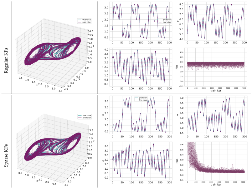
Figure 1: A comparison of learned phase, trajectories, and loss for the BeerRNN system.

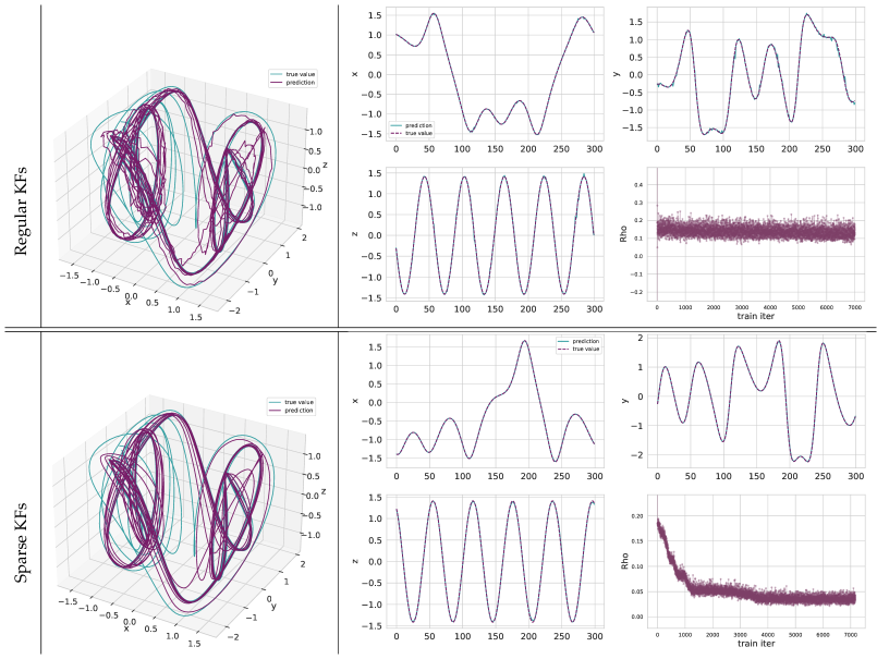
Figure 2: A comparison of learned phase, trajectories, and loss for the Duffing system.

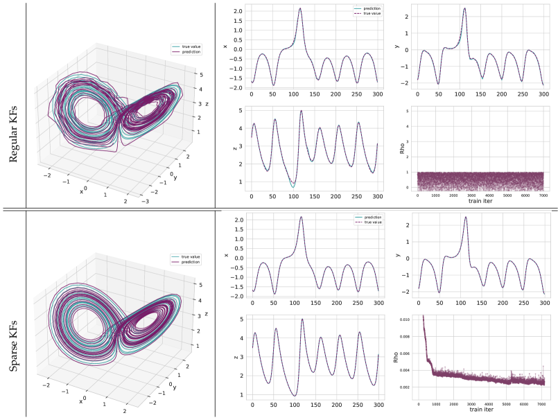
Figure 3: A comparison of learned phase, trajectories, and loss for the Lorenz system.

Table 1: Forecasting errors obtained by the Regular KFs and Sparse KFs

name	Regular KFs		Sparse KFs
	SMAPE	HD	SMAPE	HD
BeerRNN	0.0284	0.1164	0.0048	0.0333
Duffing	0.0560	0.0425	0.0075	0.0043
Lorenz	0.0372	0.0130	0.0097	0.0056

Table 2: Weight coefficients of kernel obtained by the Regular KFs and Sparse KFs

Coefficient	BeerRNN		Duffing		Lorenz
	Regular	Sparse	Regular	Sparse	Regular	Sparse
$\alpha_{1}$	0.5746	0	0.7285	0	0.7341	0
$\alpha_{2}$	0.4692	0.9985	0.7310	0.0242	0.7284	0.9918
$\alpha_{3}$	0.7234	0	0.7170	0.6807	0.7341	0
$\alpha_{4}$	0.7316	0	0.7238	0	0.7355	0
$\alpha_{5}$	0.7474	0	0.7008	0	0.7298	0
$\alpha_{6}$	0.7180	0	0.8214	0	0.6484	0
$\alpha_{7}$	0.7448	0	0.7234	0	0.7442	0.2498
$\alpha_{8}$	0.8351	0	0.7272	0	0.7206	0
$\alpha_{9}$	0.8604	0.9998	0.7658	0	0.7450	0
$\alpha_{10}$	0.7660	0	0.7239	0	0.7362	0
$\alpha_{11}$	0.7343	0	0.7265	0	0.7376	0
$\alpha_{12}$	0.7527	0	0.7310	0	0.7346	0.2785
$\alpha_{13}$	0.7337	0	0.7063	0	0.7391	0
$\alpha_{14}$	0.7322	0	0.7116	0	0.7351	0
$\alpha_{15}$	0.7398	0	0.7027	0	0.7433	0
$\alpha_{16}$	0.7363	0	0.7031	0	0.7333	0
$\alpha_{17}$	0.7052	0	0.7131	0	0.7506	0
$\alpha_{18}$	0.6815	0	0.6978	0	0.7497	0
$\alpha_{19}$	0.6959	0.8630	0.7676	0	0.7343	0
$\alpha_{20}$	0.7305	1	0.7789	0	0.6839	0
$\alpha_{21}$	0.7321	0	0.7303	0	0.7310	0

3.4 Comparison with baseline methods

In order to further demonstrate the performance of the method, we make a comparison with several baseline methods, including kernel regression with Gaussian kernel ($\sigma=0.5$) and trained Gaussian kernel by regular KFs. For the convenience of presentation, the two methods are abbreviated to “RBF”, and “Trained RBF”, respectively. The comparison results are summarized at Figure 4 and Table 2.

On the basis of the results, we may roughly conclude the following: Figure 4 presents the forecasting performance of four methods, and every box depicts the distribution of forecasting errors for all 132 dynamical systems. From the statistical perspective, the performance of the four methods can be summarized as

$$\text{RBF}\prec\text{Trained RBF}\prec\text{Regular KFs}\prec\text{RBF}$$

Specifically, Table 2 shows the detailed forecasting errors. In terms of the SMAPE criterion, in 120 dynamical systems, Sparse KFs has the smallest SMPEs, indicating adaptive kernel provides more precious forecasts. The Trained RBF performs best in 9 systems, partially indicating the kernel learning methods could improve the forecasting performance of kernel regression. In addition, there are 3 systems which Regular Kfs performs best with smallest SMAPEs.

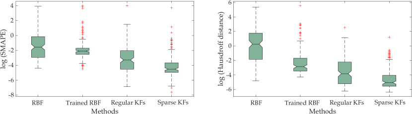
Figure 4: Distribution of forecasting errors for different methods for all 132 dynamical systems.

Table 2: one-head forecasting errors for 132 chaotic dynamical systems
Name	RBF Kernel		Trained RBF Kernel		Regular KFs		Sparse KFs		Best
	SMAPE	HD	SMAPE	HD	SMAPE	HD	SMAPE	HD
Aizawa	0.2186	1.2855	0.2049	0.0244	0.0683	0.0081	0.0322	0.0027	Sparse KFs
AnishchenkoAstakhov	0.1554	2.2373	0.0927	0.0507	0.0312	0.0190	0.0082	0.0030	Sparse KFs
Arneodo	0.0795	0.0472	0.1028	0.0239	0.0106	0.0086	0.0103	0.0027	Sparse KFs
ArnoldBeltramiChildress	0.0456	0.0478	0.1443	0.0297	0.0832	0.0179	0.0764	0.0173	Trained RBF
ArnoldWeb	24.2023	171.4064	48.4955	262.1925	0.0391	0.1522	0.0160	0.2081	Sparse KFs
AtmosphericRegime	0.4452	0.6260	0.6062	0.4058	0.5512	0.7474	0.5168	0.3314	Sparse KFs
BeerRNN	0.3792	10.1832	0.1477	0.2636	0.0284	0.1164	0.0048	0.0333	Sparse KFs
BelousovZhabotinsky	0.1022	215.8174	0.1203	6.1369	0.1610	0.1173	0.0096	0.0304	Sparse KFs
BickleyJet	0.0159	0.0770	0.0833	0.0620	0.0384	0.0311	0.0043	0.0065	Sparse KFs
Blasius	0.0627	1.0313	0.0242	0.0468	0.0092	0.0089	0.0083	0.0061	Sparse KFs
BlinkingRotlet	0.7304	0.9160	0.7737	0.4399	0.7327	0.8686	0.2059	0.4307	Trained RBF
BlinkingVortex	1.4024	0.8494	1.6182	0.5333	0.7504	0.5914	0.5423	0.5566	Trained RBF
Bouali	0.2115	4.5773	0.0794	0.0584	0.1644	0.1649	0.0057	0.0075	Sparse KFs
Bouali2	0.1604	3.6113	0.0468	0.0411	0.0010	0.0355	0.0034	0.0086	Sparse KFs
BurkeShaw	1.0260	5.2350	0.0879	0.0648	0.0123	0.0052	0.0099	0.0034	Sparse KFs
CaTwoPlus	0.0188	0.3077	0.0148	0.0908	0.0025	0.0220	0.0011	0.0119	Sparse KFs
CaTwoPlusQuasiperiodic	0.0263	0.1421	0.0240	0.1012	0.0022	0.0175	0.0005	0.0049	Sparse KFs
CellCycle	1.3828	15.5649	0.0236	0.1439	0.0144	0.1163	0.0049	0.0228	Sparse KFs
CellularNeuralNetwork	0.0499	0.0132	0.1462	0.0307	0.8356	0.2267	0.0326	0.0088	RBF
Chen	0.7046	12.0451	0.0736	0.0776	0.0100	0.0073	0.0125	0.0066	Sparse KFs
ChenLee	0.0813	0.1641	0.1314	0.0568	0.3262	0.0269	0.0075	0.0036	Sparse KFs
Chua	0.0388	0.0122	0.1237	0.0287	0.0188	0.0068	0.0031	0.0064	RBF
CircadianRhythm	0.2496	2.5516	0.2166	0.0587	0.0725	0.0735	0.1488	0.0418	Sparse KFs
CoevolvingPredatorPrey	0.2718	4.5867	0.3627	0.0489	0.1599	0.1538	0.0190	0.0460	Trained RBF
Colpitts	0.0394	0.9218	0.0608	0.1672	0.0544	0.1106	0.0019	0.0339	Sparse KFs
Coullet	0.0666	0.2871	0.0943	0.0313	0.0155	0.0095	0.0031	0.0027	Regular KFs
Dadras	1.9320	9.5681	0.3464	2.7592	0.1888	0.0612	0.0292	0.0218	Sparse KFs
DequanLi	0.2080	1.0061	0.1323	0.0296	0.0102	0.0040	0.0076	0.0034	Sparse KFs
DoubleGyre	0.1868	0.4850	0.0945	0.0364	0.1599	0.1428	0.0054	0.0077	Sparse KFs
DoublePendulum	7.5702	8.2609	0.7037	0.4982	1.0474	0.5119	0.7049	0.4731	Sparse KFs
Duffing	0.3260	0.8533	0.1883	0.0375	0.0560	0.0425	0.0075	0.0043	Sparse KFs
ExcitableCell	0.3806	83.0296	0.0582	22.1067	0.0115	0.1725	0.0011	0.0125	Sparse KFs
Finance	0.0980	1.9899	0.0523	0.0912	0.0823	0.0557	0.0095	0.0062	Sparse KFs
FluidTrampoline	0.1125	0.0568	0.2337	0.0454	0.0140	0.0189	0.0076	0.0114	Sparse KFs
ForcedBrusselator	0.0774	1.3912	0.0417	0.0644	0.0293	0.0528	0.0036	0.0109	Sparse KFs
ForcedFitzHughNagumo	0.0765	0.1537	0.1406	0.0251	0.0980	0.1159	0.0595	0.0363	Trained RBF
ForcedVanDerPol	0.1977	0.9019	0.1815	0.4087	0.7877	0.4033	0.1758	0.0333	Sparse KFs
GenesioTesi	0.0303	0.0250	0.0790	0.0229	0.0038	0.0034	0.0099	0.0035	Sparse KFs
GuckenheimerHolmes	0.3252	1.8615	0.1818	0.0189	0.0163	0.0045	0.0113	0.0021	Sparse KFs
Hadley	0.1454	1.2400	0.0958	0.0261	0.1057	0.0303	0.0070	0.0027	Sparse KFs
Halvorsen	0.0476	0.0394	0.0850	0.0278	0.8315	0.2636	0.0163	0.0036	Sparse KFs
HastingsPowell	0.0156	0.1860	0.0183	0.0814	0.0070	0.0234	0.0039	0.0093	Sparse KFs
HenonHeiles	0.0740	0.0255	0.1751	0.0339	0.0130	0.0020	0.0262	0.0020	Sparse KFs
HindmarshRose	0.1705	2.2443	0.1567	0.0941	0.1879	0.0676	0.0501	0.0121	Sparse KFs
Hopfield	0.2690	0.5214	0.2258	0.0654	0.0704	0.0859	0.0683	0.0816	Trained RBF
HyperBao	0.8635	8.3261	0.1094	0.0695	0.0971	0.0169	0.0020	0.0062	Sparse KFs
HyperCai	0.2774	3.7645	0.1040	0.0698	0.1104	0.0939	0.0073	0.0072	Sparse KFs
HyperJha	0.5032	5.8067	0.1576	0.0658	0.0825	0.0365	0.0091	0.0055	Sparse KFs
HyperLorenz	1.9790	12.2844	0.1806	0.0792	0.0166	0.0064	0.0216	0.0060	Sparse KFs
HyperLu	1.2429	10.7042	0.1245	0.0689	0.1049	0.0732	0.0074	0.0061	Sparse KFs
HyperPang	0.7841	7.2542	0.1633	0.0824	0.0473	0.0208	0.0182	0.0070	Sparse KFs
HyperQi	4.5864	19.6760	2.7646	17.6765	0.0092	0.0052	0.0096	0.0042	Sparse KFs
HyperRossler	0.8076	12.6803	0.1299	0.3022	0.2940	0.0146	0.0321	0.0066	Sparse KFs
HyperWang	1.7118	14.8686	0.1473	0.0338	0.0027	0.0026	0.0069	0.0047	Sparse KFs
HyperXu	2.2143	19.1536	0.1773	0.2483	0.0090	0.0120	0.0197	0.0077	Sparse KFs
HyperYan	1.0246	12.2693	0.2782	5.2669	0.0563	0.0265	0.0104	0.0037	Sparse KFs
HyperYangChen	1.5399	16.1034	0.1534	0.1838	0.0113	0.0068	0.0247	0.0066	Sparse KFs
IkedaDelay	4.6646	5.4753	6.3582	6.6615	1.1826	0.1482	0.2961	0.0856	Sparse KFs
IsothermalChemical	0.0235	1.3498	0.0192	0.1858	0.0044	0.0315	0.0018	0.0127	Sparse KFs
ItikBanksTumor	3.1791	1.5271	5.4786	0.0394	1.9552	0.0032	1.4649	0.0033	Sparse KFs
JerkCircuit	0.2332	1.4263	0.3403	1.0682	0.1393	0.4640	0.0815	0.2651	Sparse KFs
KawczynskiStrizhak	0.0176	0.0126	0.0405	0.0150	0.0330	0.0459	0.0029	0.0062	RBF
Laser	0.0920	0.1182	0.1116	0.0297	0.0056	0.0033	0.0046	0.0039	Sparse KFs
LiuChen	50.8445	13.2288	54.7053	11.5904	55.5113	3.1109	41.2576	0.5160	Sparse KFs
Lorenz	0.0441	0.4909	0.0684	0.0484	0.0372	0.0130	0.0097	0.0056	Sparse KFs
Lorenz84	0.2626	0.2467	0.1896	0.0322	0.1597	0.0992	0.0198	0.0047	Sparse KFs
Lorenz96	1.5382	1.7985	0.3046	0.0576	0.3691	0.1072	0.0682	0.0069	Sparse KFs
LorenzBounded	0.0685	0.4453	0.0597	0.0467	0.0217	0.0875	0.0108	0.0042	Sparse KFs
LorenzCoupled	2.0416	12.6271	0.1269	0.1778	0.0017	0.0054	0.0106	0.0077	Sparse KFs
LorenzStenflo	0.4044	7.6345	0.1226	0.0887	0.0166	0.0214	0.0236	0.0075	Sparse KFs
LuChen	0.0531	1.3090	0.0527	0.0665	0.0717	0.0318	0.0112	0.0068	Sparse KFs
LuChenCheng	0.0295	0.0643	0.0991	0.0342	0.0126	0.0161	0.0048	0.0036	Sparse KFs
MacArthur	4.2470	39.7701	0.1105	0.7623	0.0471	0.5928	0.0120	0.2382	Sparse KFs
MackeyGlass	3.4885	16.1632	0.0543	0.2721	0.0083	0.0722	0.0211	0.0713	Sparse KFs
MooreSpiegel	0.0734	0.1170	0.1194	0.0340	0.0418	0.0195	0.0120	0.0044	Sparse KFs
MultiChua	0.0255	0.0235	0.0662	0.0341	0.0050	0.0068	0.0074	0.0079	Sparse KFs
NewtonLiepnik	0.2729	1.5179	0.0777	0.0482	0.0279	0.0127	0.0080	0.0064	Sparse KFs
NoseHoover	0.2481	1.2736	0.1457	0.0472	0.0055	0.0023	0.0168	0.0031	Sparse KFs
NuclearQuadrupole	0.8340	1.3394	0.1462	0.0281	0.0307	0.0132	0.0087	0.0035	Sparse KFs
OscillatingFlow	0.7238	1.3119	0.2332	0.0722	0.1812	0.0769	0.1080	0.0362	Sparse KFs
PanXuZhou	0.0851	0.2774	0.1313	0.0493	0.0379	0.0048	0.0104	0.0046	Sparse KFs
PehlivanWei	0.2546	1.1650	0.1160	0.0385	0.0183	0.0043	0.0122	0.0027	Sparse KFs
PiecewiseCircuit	11.9312	9.5461	1.1743	1.2830	0.4631	0.3629	0.4094	0.3498	Sparse KFs
Qi	2.3154	49.6780	0.1436	1.5068	1.0231	0.3504	0.0414	0.0185	Sparse KFs
QiChen	0.1621	6.9077	0.0384	0.0619	0.1220	0.0412	0.0137	0.0099	Sparse KFs
RabinovichFabrikant	0.0308	0.0514	0.0403	0.0420	0.0058	0.0045	0.0061	0.0046	Sparse KFs
RayleighBenard	0.1740	4.0007	0.0796	0.0566	0.0086	0.0065	0.0087	0.0067	Sparse KFs
RikitakeDynamo	0.4957	5.5948	0.0868	0.0770	0.0686	0.0367	0.0101	0.0042	Sparse KFs
Rossler	0.3387	4.7017	0.1132	0.1881	0.0318	0.0034	0.0295	0.0045	Sparse KFs
Rucklidge	0.2231	2.8533	0.0956	0.0824	0.0125	0.0055	0.0142	0.0053	Sparse KFs
Sakarya	1.1720	7.4699	0.1405	0.4412	0.0126	0.0046	0.0154	0.0050	Sparse KFs
SaltonSea	0.0149	0.0643	0.0180	0.0514	0.0038	0.0086	0.0009	0.0039	Sparse KFs
SanUmSrisuchinwong	0.3718	2.4040	0.2000	0.0462	0.0393	0.0172	0.0172	0.0086	Sparse KFs
ScrollDelay	1.6963	2.1868	0.3892	0.0714	1.4291	0.1713	0.3249	0.1553	Trained RBF
ShimizuMorioka	0.0384	0.0904	0.0977	0.0408	0.0077	0.0051	0.0128	0.0048	Sparse KFs
SprottA	0.1883	0.7459	0.1464	0.0227	0.0107	0.0048	0.0150	0.0033	Sparse KFs
SprottB	1.5516	7.6672	0.1158	0.3188	0.1499	0.0434	0.0108	0.0039	Sparse KFs
SprottC	0.0647	0.4746	0.0962	0.0276	0.0080	0.0038	0.0074	0.0032	Sparse KFs
SprottD	0.2941	3.3511	0.0625	0.0472	0.0110	0.0049	0.0071	0.0048	Sparse KFs
SprottDelay	0.0332	0.2678	0.0115	0.0158	0.0565	0.3096	0.0018	0.0050	Sparse KFs
SprottE	0.0749	0.7674	0.0916	0.0312	0.0023	0.0024	0.0124	0.0042	Sparse KFs
SprottF	0.0882	0.6506	0.1148	0.0237	0.0079	0.0047	0.0083	0.0046	Regular KFs
SprottG	0.0427	0.0242	0.1096	0.0287	0.0242	0.0054	0.0155	0.0034	Sparse KFs
SprottH	0.2228	0.9717	0.1818	0.0444	0.0139	0.0055	0.0178	0.0051	Sparse KFs
SprottI	0.0302	0.0316	0.0672	0.0241	0.0517	0.0490	0.0055	0.0038	Sparse KFs
SprottJ	0.0175	0.0141	0.0685	0.0189	0.1167	0.0140	0.0090	0.0031	Sparse KFs
SprottJerk	0.0535	0.3400	0.1402	0.0167	0.0449	0.0042	0.0149	0.0042	Sparse KFs
SprottK	0.0884	0.2206	0.1267	0.0244	0.0168	0.0034	0.0095	0.0030	Sparse KFs
SprottL	0.0314	0.0744	0.0441	0.0474	0.0041	0.0138	0.0059	0.0083	Sparse KFs
SprottM	0.0468	0.0187	0.0714	0.0266	0.0101	0.0036	0.0094	0.0034	Sparse KFs
SprottMore	1.3180	1.7383	2.0323	0.5184	0.6949	0.3744	0.3135	0.3061	Sparse KFs
SprottN	0.0266	0.0081	0.1237	0.0138	0.0870	0.0216	0.0201	0.0035	Sparse KFs
SprottO	0.0373	0.0191	0.1060	0.0274	0.0169	0.0049	0.0120	0.0024	Sparse KFs
SprottP	0.0471	0.1090	0.1495	0.0227	0.0096	0.0055	0.0065	0.0018	Sparse KFs
SprottQ	0.0541	0.0408	0.0962	0.0234	0.0142	0.0034	0.0037	0.0017	Sparse KFs
SprottR	0.1182	1.2301	0.1157	0.0314	0.0390	0.0303	0.0122	0.0046	Sparse KFs
SprottS	0.0436	0.0215	0.1422	0.0283	0.0121	0.0049	0.0072	0.0033	Sparse KFs
SprottTorus	1.8440	13.5801	2.0916	11.7551	0.0062	0.0174	0.0068	0.0262	Regular KFs
StickSlipOscillator	0.0149	0.0223	0.1144	0.0647	0.0060	0.0048	0.0025	0.0032	Sparse KFs
SwingingAtwood	1.3206	5.9341	0.2365	0.4268	0.1911	0.9231	0.0878	0.3789	Sparse KFs
Thomas	0.0964	0.0221	0.1858	0.0187	0.6922	0.1694	0.0188	0.0074	Trained RBF
ThomasLabyrinth	1.1063	2.0744	1.4589	0.1824	2.3277	0.3354	0.5611	0.2008	Trained RBF
Torus	0.0125	0.0823	0.0282	0.1320	0.0497	0.3391	0.0037	0.0104	Sparse KFs
Tsucs2	0.8522	4.5254	0.1237	0.1248	0.0064	0.0021	0.0276	0.0051	Sparse KFs
TurchinHanski	0.2858	1.9826	0.1663	0.0357	0.0299	0.0195	0.0247	0.0178	Sparse KFs
VallisElNino	0.0407	0.0839	0.0703	0.0197	0.0408	0.0258	0.0118	0.0037	Sparse KFs
VossDelay	37.9067	19.0553	38.4574	18.7339	4.5635	12.6397	3.1540	3.3905	Sparse KFs
WangSun	1.9833	10.1195	0.5392	4.1739	1.9652	1.4283	0.0394	0.0252	Sparse KFs
WindmiReduced	0.0584	0.8784	0.1360	1.9927	0.0158	0.6915	0.0096	0.2036	Sparse KFs
YuWang	0.3932	5.6805	0.1470	0.2048	0.0371	0.1076	0.1190	0.0828	Sparse KFs
YuWang2	0.0360	0.1737	0.0490	0.0474	0.0078	0.0256	0.0051	0.0128	Sparse KFs
ZhouChen	4.5703	25.6922	3.2739	18.4165	0.2694	0.0129	0.2194	0.0134	Sparse KFs

4 Conclusion

In this work, we present a Sparse Kernel Flows algorithm for learning the ’best’ kernel from data. The proposal provides an effective modification of the method of Regular Kernel Flows that allows sparsifying the initial base kernel and improves the accuracy. Our numerical experiments on a benchmark of 132 chaotic systems demonstrate that the learned kernel using Sparse Kernel Flows is able to accurately represent the underlying dynamical system responsible for generating the time series data.

Appendix A Appendix

A.1 Reproducing Kernel Hilbert Spaces (RKHS)

We give a brief overview of reproducing kernel Hilbert spaces as used in statistical learning theory  [13]. Early work developing the theory of RKHS was undertaken by N. Aronszajn [4].

Definition 1.

Let ${\mathcal{H}}$ be a Hilbert space of functions on a set ${\mathcal{X}}$. Denote by $\langle f,g\rangle$ the inner product on ${\mathcal{H}}$ and let $\|f\|=\langle f,f\rangle^{1/2}$ be the norm in ${\mathcal{H}}$, for $f$ and $g\in{\mathcal{H}}$. We say that ${\mathcal{H}}$ is a reproducing kernel Hilbert space (RKHS) if there exists a function $k:{\mathcal{X}}\times{\mathcal{X}}\rightarrow\mathbb{R}$ such that

• $k_{x}:=k(x,\cdot)\in{\mathcal{H}}$ for all $x\in{\mathcal{H}}$.

• $k$ spans ${\mathcal{H}}$: ${\mathcal{H}}=\overline{\mbox{span}\{k_{x}~{}|~{}x\in{\mathcal{X}}\}}$.

• $k$ has the reproducing property: $\forall f\in{\mathcal{H}}$, $f(x)=\langle f,k_{x}\rangle$.

$k$ will be called a reproducing kernel of ${\mathcal{H}}$. ${\mathcal{H}}_{k}$ will denote the RKHS ${\mathcal{H}}$ with reproducing kernel $k$ where it is convenient to explicitly note this dependence.

The important properties of reproducing kernels are summarized in the following proposition.

Proposition 1.

If $k$ is a reproducing kernel of a Hilbert space ${\mathcal{H}}$, then

• $k(x,y)$ is unique.

• $\forall x,y\in{\mathcal{X}}$, $k(x,y)=k(y,x)$ (symmetry).

• $\sum_{i,j=1}^{q}\alpha_{i}\alpha_{j}k(x_{i},x_{j})\geq 0$ for $\alpha_{i}\in\mathbb{R}$, $x_{i}\in{\mathcal{X}}$ and $q\in\mathbb{N}_{+}$ (positive definiteness).

• $\langle k(x,\cdot),k(y,\cdot)\rangle=K(x,y)$.

Common examples of reproducing kernels defined on a compact domain $\mathcal{X}\subset\mathrm{R}^{n}$ are the (1) constant kernel: $K(x,y)=m>0$ (2) linear kernel: $k(x,y)=x\cdot y$ (3) polynomial kernel: $k(x,y)=(1+x\cdot y)^{d}$ for $d\in\mathbb{N}_{+}$ (4) Laplace kernel: $k(x,y)=e^{-||x-y||_{2}/\sigma^{2}}$, with $\sigma>0$ (5) Gaussian kernel: $k(x,y)=e^{-||x-y||^{2}_{2}/\sigma^{2}}$, with $\sigma>0$ (6) triangular kernel: $k(x,y)=\max\{0,1-\frac{||x-y||_{2}^{2}}{\sigma}\}$, with $\sigma>0$. (7) locally periodic kernel: $k(x,y)=\sigma^{2}e^{-2\frac{\sin^{2}(\pi||x-y||_{2}/p)}{\ell^{2}}}e^{-\frac{||x-y||_{2}^{2}}{2\ell^{2}}}$, with $\sigma,\ell,p>0$.

Theorem 1.

Let $k:{\mathcal{X}}\times{\mathcal{X}}\rightarrow\mathbb{R}$ be a symmetric and positive definite function. Then there exists a Hilbert space of functions ${\mathcal{H}}$ defined on ${\mathcal{X}}$ admitting $k$ as a reproducing Kernel. Conversely, let ${\mathcal{H}}$ be a Hilbert space of functions $f:{\mathcal{X}}\rightarrow\mathbb{R}$ satisfying $\forall x\in{\mathcal{X}},\exists\kappa_{x}>0,$ such that $|f(x)|\leq\kappa_{x}\|f\|_{\mathcal{H}},\quad\forall f\in{\mathcal{H}}.$ Then ${\mathcal{H}}$ has a reproducing kernel $k$.

Theorem 2.

Let $k(x,y)$ be a positive definite kernel on a compact domain or a manifold $X$. Then there exists a Hilbert space $\mathcal{F}$ and a function $\Phi:X\rightarrow\mathcal{F}$ such that

$$k(x,y)=\langle\Phi(x),\Phi(y)\rangle_{\mathcal{F}}\quad\mbox{for}\quad x,y\in X.$$

$\Phi$ is called a feature map, and $\mathcal{F}$ a feature space.

Data accessibility

Data and codes are available at https://github.com/Yanglu0319/Sparse_Kernel_Flows.

References

- Abarbanel [2012] Abarbanel, H., 2012. Analysis of Observed Chaotic Data. Institute for Nonlinear Science, Springer New York.
- Akian et al. [2022] Akian, J.L., Bonnet, L., Owhadi, H., Savin, É., 2022. Learning “best” kernels from data in Gaussian process regression. With application to aerodynamics. Journal of Computational Physics 470, 111595. doi:10.1016/j.jcp.2022.111595.
- Alexander and Giannakis [2020] Alexander, R., Giannakis, D., 2020. Operator-theoretic framework for forecasting nonlinear time series with kernel analog techniques. Physica D: Nonlinear Phenomena 409, 132520. URL: http://www.sciencedirect.com/science/article/pii/S016727891930377X, doi:https://doi.org/10.1016/j.physd.2020.132520.
- Aronszajn [1950] Aronszajn, N., 1950. Theory of reproducing kernels. Transactions of the American Mathematical Society 68, 337–404. URL: http://dx.doi.org/10.2307/1990404.
- Bottou [2012] Bottou, L., 2012. Stochastic Gradient Descent Tricks, in: Montavon, G., Orr, G.B., Müller, K.R. (Eds.), Neural Networks: Tricks of the Trade: Second Edition. Springer, Berlin, Heidelberg. Lecture Notes in Computer Science, pp. 421–436. doi:10.1007/978-3-642-35289-8_25.
- Bouvrie and Hamzi [2012] Bouvrie, J., Hamzi, B., 2012. Empirical estimators for stochastically forced nonlinear systems: Observability, controllability and the invariant measure. Proc. of the 2012 American Control Conference , 294–301https://arxiv.org/abs/1204.0563v1.
- Bouvrie and Hamzi [2017a] Bouvrie, J., Hamzi, B., 2017a. Kernel methods for the approximation of nonlinear systems. SIAM J. Control and Optimization https://arxiv.org/abs/1108.2903.
- Bouvrie and Hamzi [2017b] Bouvrie, J., Hamzi, B., 2017b. Kernel methods for the approximation of some key quantities of nonlinear systems. Journal of Computational Dynamics 1. http://arxiv.org/abs/1204.0563.
- Brunton et al. [2016] Brunton, S.L., Proctor, J.L., Kutz, J.N., 2016. Discovering governing equations from data by sparse identification of nonlinear dynamical systems. Proceedings of the National Academy of Sciences 113, 3932–3937. URL: https://www.pnas.org/content/113/15/3932, doi:10.1073/pnas.1517384113, arXiv:https://www.pnas.org/content/113/15/3932.full.pdf.
- Casdagli [1989] Casdagli, M., 1989. Nonlinear prediction of chaotic time series. Physica D: Nonlinear Phenomena 35, 335 -- 356. URL: http://www.sciencedirect.com/science/article/pii/0167278989900742, doi:https://doi.org/10.1016/0167-2789(89)90074-2.
- Chattopadhyay et al. [2019] Chattopadhyay, A., Hassanzadeh, P., Palem, K.V., Subramanian, D., 2019. Data-driven prediction of a multi-scale lorenz 96 chaotic system using a hierarchy of deep learning methods: Reservoir computing, ann, and RNN-LSTM. CoRR abs/1906.08829. URL: http://arxiv.org/abs/1906.08829, arXiv:1906.08829.
- Chen et al. [2021] Chen, Y., Hosseini, B., Owhadi, H., Stuart, A.M., 2021. Solving and learning nonlinear PDEs with Gaussian processes. Journal of Computational Physics 447, 110668. doi:10.1016/j.jcp.2021.110668.
- Cucker and Smale [2002] Cucker, F., Smale, S., 2002. On the mathematical foundations of learning. Bulletin of the American Mathematical Society 39, 1--49.
- Darcy et al. [2023] Darcy, M., Hamzi, B., Susiluoto, J., Braverman, A., Owhadi, H., 2023. Learning dynamical systems from data: a simple cross-validation perspective, part II: nonparametric kernel flows. Physica D 444, 133583. URL: https://www.researchgate.net/publication/356818178_Learning_dynamical_systems_from_data_a_simple_cross-validation_perspective_part_II_nonparametric_kernel_flows.
- Darcy et al. [2021] Darcy, M., Tavallali, P., Livieri, G., Hamzi, B., Owhadi, H., 2021. One-shot learning of stochastic differential equations with computational graph completion. preprint URL: https://www.researchgate.net/profile/Boumediene-Hamzi/publication/358263232_One-Shot_Learning_of_Stochastic_Differential_Equations_with_Computational_Graph_Completion/links/61f8fd2b11a1090a79c707ca/One-Shot-Learning-of-Stochastic-Differential-Equations-with-Computational-Graph-Completion.pdf.
- D.Wittwar [2021] D.Wittwar, B.B..G.., 2021. Kernel methods for center manifold approximation and a weak data-based version of the center manifold theorems. Physica D .
- Exterkate et al. [2016] Exterkate, P., Groenen, P.J.F., Heij, C., van Dijk, D., 2016. Nonlinear forecasting with many predictors using kernel ridge regression. International Journal of Forecasting 32, 736--753. doi:10.1016/j.ijforecast.2015.11.017.
- Giesl et al. [2019] Giesl, P., Hamzi, B., Rasmussen, M., Webster, K., 2019. Approximation of Lyapunov functions from noisy data. Journal of Computational Dynamics doi:10.3934/jcd.2020003. https://arxiv.org/abs/1601.01568.
- Gilpin [2021] Gilpin, W., 2021. Chaos as an interpretable benchmark for forecasting and data-driven modelling. arXiv:2110.05266.
- González-García et al. [1998] González-García, R., Rico-Martínez, R., Kevrekidis, I., 1998. Identification of distributed parameter systems: A neural net based approach. Computers & Chemical Engineering 22, S965--S968. URL: https://www.sciencedirect.com/science/article/pii/S0098135498001914, doi:https://doi.org/10.1016/S0098-1354(98)00191-4. european Symposium on Computer Aided Process Engineering-8.
- Grandstrand [1995] Grandstrand, O., 1995. Nonlinear system identification using neural networks: dynamics and instanbilities, in: Bulsari, A.B. (Ed.), Neural Networks for Chemical Engineers. Elsevier, Elsevier. chapter 16, pp. 409--442.
- Haasdonk et al. [2018] Haasdonk, B., Hamzi, B., Santin, G., Wittwar, D., 2018. Greedy kernel methods for center manifold approximation. Proc. of ICOSAHOM 2018, International Conference on Spectral and High Order Methods https://arxiv.org/abs/1810.11329.
- Hamzi and Colonius [2019] Hamzi, B., Colonius, F., 2019. Kernel methods for the approximation of discrete-time linear autonomous and control systems. SN Applied Sciences 1, 674. doi:10.1007/s42452-019-0701-3.
- Hamzi et al. [2019] Hamzi, B., Kuehn, C., Mohamed, S., 2019. A note on kernel methods for multiscale systems with critical transitions. Mathematical Methods in the Applied Sciences 42, 907--917. URL: https://onlinelibrary.wiley.com/doi/abs/10.1002/mma.5394, doi:https://doi.org/10.1002/mma.5394, arXiv:https://onlinelibrary.wiley.com/doi/pdf/10.1002/mma.5394.
- Hamzi et al. [2022] Hamzi, B., Maulik, R., Owhadi, H., 2022. Simple, low-cost and accurate data-driven geophysical forecasting with learned kernels. Proceedings of the Royal Society A: Mathematical, Physical and Engineering Sciences , 18.
- Hamzi and Owhadi [2021a] Hamzi, B., Owhadi, H., 2021a. Learning dynamical systems from data: A simple cross-validation perspective, part i: Parametric kernel flows. Physica D: Nonlinear Phenomena 421, 132817. URL: https://www.sciencedirect.com/science/article/pii/S0167278920308186, doi:https://doi.org/10.1016/j.physd.2020.132817.
- Hamzi and Owhadi [2021b] Hamzi, B., Owhadi, H., 2021b. Learning dynamical systems from data: A simple cross-validation perspective, part I: Parametric kernel flows. Physica D: Nonlinear Phenomena 421, 132817. doi:10.1016/j.physd.2020.132817.
- Hamzi et al. [2023] Hamzi, B., Owhadi, H., Kevrekidis, Y., 2023. Learning dynamical systems from data: A simple cross-validation perspective, part iv: case with partial observations .
- Hudson et al. [1990] Hudson, J., Kube, M., Adomaitis, R., Kevrekidis, I., Lapedes, A., Farber, R., 1990. Nonlinear signal processing and system identification: applications to time series from electrochemical reactions. Chemical Engineering Science 45, 2075--2081. URL: https://www.sciencedirect.com/science/article/pii/000925099080079T, doi:https://doi.org/10.1016/0009-2509(90)80079-T.
- Jung [2018] Jung, Y., 2018. Multiple predicting K-fold cross-validation for model selection. Journal of Nonparametric Statistics 30, 197--215. doi:10.1080/10485252.2017.1404598.
- Kantz and Schreiber [1997] Kantz, H., Schreiber, T., 1997. Nonlinear Time Series Analysis. Cambridge University Press, USA.
- Klus et al. [2020a] Klus, S., Nüske, F., Hamzi, B., 2020a. Kernel-based approximation of the koopman generator and schrödinger operator. Entropy 22, 722.
- Klus et al. [2020b] Klus, S., Nuske, F., Hamzi, B., 2020b. Kernel-based approximation of the koopman generator and schrödinger operator. Entropy 22. https://www.mdpi.com/1099-4300/22/7/722.
- Klus et al. [2020c] Klus, S., Nüske, F., Peitz, S., Niemann, J.H., Clementi, C., Schütte, C., 2020c. Data-driven approximation of the koopman generator: Model reduction, system identification, and control. Physica D: Nonlinear Phenomena 406, 132416.
- Koltai, and Schutte [2019] Koltai,, A.B.S.K.B.H.P., Schutte, C., 2019. Dimensionality reduction of complex metastable systems via kernel embeddings of transition manifold. Https://arxiv.org/abs/1904.08622.
- Lee et al. [2021] Lee, J., De Brouwer, E., Hamzi, B., Owhadi, H., 2021. Learning dynamical systems from data: A simple cross-validation perspective, part III: Irregularly-Sampled Time Series. arXiv:2111.13037.
- Lu et al. [2023] Lu, Y., Hamzi, B., Owhadi, H., Kevrekidis, Y., Xiuwen, S., Naiming, X., 2023. Learning dynamical systems from data: A simple cross-validation perspective, part vii: Hausdroff distance .
- Nielsen [2019] Nielsen, A., 2019. Practical Time Series Analysis: Prediction with Statistics and Machine Learning. O’Reilly Media.
- Owhadi [2021a] Owhadi, B.H..R.M.H., 2021a. Simple, low-cost and accurate data-driven geophysical forecasting with learned kernels. Proceedings of the Royal Society A: Mathematical, Physical and Engineering Sciences 477(2252). doi:10.1098/rspa.2021.0326.
- Owhadi [2021b] Owhadi, H., 2021b. Computational graph completion URL: https://arxiv.org/abs/2110.10323, doi:10.48550/ARXIV.2110.10323.
- Owhadi and Scovel [2019] Owhadi, H., Scovel, C., 2019. Operator-Adapted Wavelets, Fast Solvers, and Numerical Homogenization: from a game theoretic approach to numerical approximation and algorithm design. Cambridge Monographs on Applied and Computational Mathematics, Cambridge University Press.
- Owhadi and Yoo [2019a] Owhadi, H., Yoo, G.R., 2019a. Kernel flows: From learning kernels from data into the abyss. Journal of Computational Physics 389, 22--47. doi:10.1016/j.jcp.2019.03.040.
- Owhadi and Yoo [2019b] Owhadi, H., Yoo, G.R., 2019b. Kernel Flows: From learning kernels from data into the abyss. Journal of Computational Physics 389, 22--47. doi:10.1016/j.jcp.2019.03.040.
- Pathak et al. [2017] Pathak, J., Lu, Z., Hunt, B.R., Girvan, M., Ott, E., 2017. Using machine learning to replicate chaotic attractors and calculate lyapunov exponents from data. Chaos: An Interdisciplinary Journal of Nonlinear Science 27, 121102. URL: https://doi.org/10.1063/1.5010300, doi:10.1063/1.5010300.
- Rico-Martinez et al. [1992] Rico-Martinez, R., Krischer, K., Kevrekidis, I., Kube, M., Hudson, J., 1992. Discrete-vs. continuous-time nonlinear signal processing of cu electrodissolution data. Chemical Engineering Communications 118, 25--48.
- Santin and Haasdonk [2019] Santin, G., Haasdonk, B., 2019. Kernel methods for surrogate modeling https://arxiv.org/abs/1907.105566.
- Tibshirani [1996] Tibshirani, R., 1996. Regression Shrinkage and Selection Via the Lasso. Journal of the Royal Statistical Society: Series B (Methodological) 58, 267--288. doi:10.1111/j.2517-6161.1996.tb02080.x.
- Yasamin et al. [2023] Yasamin, J., Hamzi, B., Owhadi, H., Peyman, T., Moustafa, S., 2023. Learning dynamical systems from data: A simple cross-validation perspective, part vi: Hamiltonian systems .
- Yoo and Owhadi [2021] Yoo, G.R., Owhadi, H., 2021. Deep regularization and direct training of the inner layers of Neural Networks with Kernel Flows. Physica D: Nonlinear Phenomena 426, 132952. doi:10/gnrnn5.