On a Finite Population Variation of the Fisher-KPP Equation

Abstract

In this paper, we formulate a finite population variation of the Fisher-KPP equation using the fact that the reaction term can be generated from the replicator dynamic using a two-player two-strategy skew-symmetric game. We use prior results from Ablowitz and Zeppetella to show that the resulting system of partial differential equations admits a travelling wave solution, and that there are closed form solutions for this travelling wave. Interestingly, the closed form solution is constructed from a sign-reversal of the known closed form solution of the classic Fisher equation. We also construct a closed form solution approximation for the corresponding equilibrium problem on a finite interval with Dirichlet and Neumann boundary conditions. Two conjectures on these corresponding equilibrium problems are presented and analysed numerically.

I Introduction

Fisher [1] proposed the following equation

$$\frac{\partial u}{\partial t}=ru(1-u)+\frac{\partial^{2}u}{\partial x^{2}}$$ (1)

as a model of the propagation of a mutant genes. At (approximately) the same time, Kolmogorov, Petrovsky and Piskunov analysed a more general version of Eq. 1 [2] with $ru(1-u)$ replaced by a generic function $F(u)$ having prerequisite smoothness and end point properties. Throughout this paper, we refer to Eq. 1 as the Fisher-KPP equation. This equation is known to appear in simple models of susceptible-infected (SI) spatial epidemics with drift [3, 4, 5]. It also emerges naturally (often as a simplification) in branching processes [6], for modelling the spread of invasive species [7] and in flame propagation and combustion [8] among other areas.

Solutions (especially travelling wave solutions) to the Fisher-KPP equation have been studied by several authors. Fisher himself studied the existence of wave solutions [1] as did Kolmogorov, Petrovsky and Piskunov [2]. Kametka [9] and Uchiyama [10] studied the asymptotic formation of travelling wave solutions. Later, Newman [11] studied exact solutions. Relevant and related to the brief analysis presented here, Weinberger analysed a discrete form of the Fisher-KPP equation [12]. However, the most relevant result for this work is from Ablowitz and Zeppetella [13] who provide an explicit solution for the Fisher-KPP equation.

The objective of this paper is to construct a system of partial differential equations modelling both the propagation of a dominant species (allele, infective, competitor etc.) in the presence of a (finite) population experiencing its own spatial evolution. We do so by using a recent formulation by Griffin, Mummah and DeForest for a finite population spatial replicator equation [14]. This work extends earlier work by (among others) Vickers [15] who the studied the spatial replicator with an (assumed) infinite population and work by Durrett and Levin [16] who compared discrete and spatial population dynamics to continuous population dynamics. We show that this system of partial differential equations admits all the travelling wave solutions of the Fisher-KPP equation, except with directions reversed. We use this fact and the results from [13] to derive an explicit example and interpret it in a physical context. We then study the corresponding equilibrium problem for this equation system on a finite interval. We derive a closed form approximation for the Dirichlet problem and use it to construct a conjecture on solution behaviours as the spatial gradient of the population becomes large. A simpler problem with Neumann boundary conditions is also briefly considered.

The remainder of this paper is organized as follows: We derive the model to be studied in Section II. In Section III we show that travelling wave solutions exist and construct an explicit example. We study the equilibrium problem for the equation system in Section IV, constructing a closed form approximation for the problem with Dirichlet boundary conditions as well as two conjectures (to be proven in future work). Conclusions and future directions are presented in Section V.

II Model Derivation

The classic Fisher-KPP equation, Eq. 1, can be derived as an example of the one-dimensional infinite population spatial replicator equation

$$\frac{\partial u_{i}}{\partial t}=u_{i}\left(\mathbf{e}_{i}-\mathbf{u}\right)^{T}\mathbf{A}\mathbf{u}+k\frac{\partial^{2}u_{i}}{\partial x^{2}},$$ (2)

with skew-symmetric payoff matrix,

$$\mathbf{A}=\begin{bmatrix}0&-r\\ r&0\end{bmatrix}.$$ (3)

Here $\mathbf{u}=\langle{u_{1},u_{2}}\rangle$ and $k$ is a diffusion constant. With this payoff matrix $\mathbf{u}^{T}\mathbf{A}\mathbf{u}=0$. Focusing on the equation for $u_{2}$, we can write:

$$\frac{\partial u_{2}}{\partial t}=ru_{2}u_{1}+k\frac{\partial^{2}u_{2}}{\partial x^{2}}.$$ (4)

From [14] we know that for all $(x,t)$ we have $u_{1}+u_{2}=1$. Therefore, when $i=2$, we recover the Fisher-KPP equation

$$\frac{\partial u_{2}}{\partial t}=ru_{2}(1-u_{2})+k\frac{\partial^{2}u_{2}}{\partial x^{2}},$$ (5)

which can simply be written as Eq. 1 with no subscripts and assuming $k=1$.

In [14] is it shown that for finite populations, the spatial replicator is given by the system of equations

$$\forall r\left\{\begin{aligned} \frac{\partial u_{r}}{\partial t}=u_{r}\cdot\left(\mathbf{e}_{r}^{T}\mathbf{A}\mathbf{u}-\mathbf{u}^{T}\mathbf{A}\mathbf{u}\right)+k\left(\frac{2}{M}\nabla M\cdot\nabla u_{r}+\Delta u_{r}\right)\end{aligned}\right.$$

$$\frac{\partial M}{\partial t}=M\mathbf{u}^{T}\mathbf{A}\mathbf{u}+k\Delta M.$$

Here $M(x,t)>0$ is the total population of all species at $(x,t)$. If $M\to\infty$ and $\partial_{x}M$ is bounded or $\partial_{x}M=0$, and we restrict to one dimension, then this equation is identical to Eq. 2. Using the payoff matrix defined in Eq. 3 and restricting to one dimension, we obtain the one dimensional finite population Fisher-KPP system

$$\left\{\begin{aligned} \frac{\partial u}{\partial t}&=ru(1-u)+\frac{2k}{M}\frac{\partial M}{\partial x}\frac{\partial u}{\partial x}+k\frac{\partial^{2}u}{\partial x^{2}}\\ \frac{\partial M}{\partial t}&=k\frac{\partial^{2}M}{\partial x^{2}}.\end{aligned}\right.$$ (6)

The population equation is simply a diffusion equation and so (without boundary or initial conditions) we are free to choose any suitable solution. We can use this to find a travelling wave solution to the system of equations, and consequently a closed form solution.

III Travelling Wave Solution

The population (diffusion) equation has a travelling wave solution given by

$$M(x,t)=\pm\frac{A}{c}\exp\left[\pm c(x\pm kct)\right]+B,$$ (7)

where $A$ and $B$ are arbitrary constants. Assume $B=0$. Then

$$\frac{1}{M}\frac{\partial M}{\partial x}=\pm c.$$ (8)

Let $k=1$ and let $z=x\pm ct$. A travelling wave solution for $u$ can be found by solving

$$\pm cu^{\prime}=ru(1-u)\pm 2cu^{\prime}+u^{\prime\prime},$$ (9)

assuming $\lim_{x\to\infty}u(x)=0$ and $\lim_{x\to-\infty}u(x)=1$, following [13]. Simplifying yields

$$ru(1-u)\pm cu^{\prime}+u^{\prime\prime}=0.$$ (10)

The travelling wave differential equation for Eq. 1 (the Fisher-KPP equation) is

$$ru(1-u)\mp cu^{\prime}+u^{\prime\prime}=0.$$ (11)

This is identical to Eq. 10 except for the sign of the $cu^{\prime}$ term, which is reversed. Therefore, the finite and infinite population equations must share travelling wave solutions but with their directions of travel reversed, assuming the total population is given by Eq. 7.

If we rescale so that $r=1$, then the (astounding) results of Ablowitz and Zeppetella [13] imply, for the special wave speed of:

$$c=\pm\frac{5}{\sqrt{6}},$$ (12)

we have the fully closed form solution:

$$u(z)=\left[1+C\exp\left(\pm\frac{z}{\sqrt{6}}\right)\right]^{-2},$$ (13)

where $C$ is another arbitrary constant. We note the solution differs from that in [13] exactly in the sign of $z$, as a result of the introduction of the finite population term. As we require $M(x,t)>0$, it follows that there is only one acceptable solution when $c>0$. This is illustrated in Fig. 1.

Figure 1: (Top) The travelling wave solution $u(x,t)$ given by Eq. 13 assuming $c>0$ given by Eq. 12 and $k=1$. (Bottom) The travelling wave solution for the population $M(x,t)$ with $k=1$ and $c>0$ given by Eq. 12. For scaling, we set $A=10^{-5}$.

In both figures, slices are at $t=\in\{0,1,2,3\}$.

The result is biologically interesting because Ablowitz and Zeppetella’s construction assumes that $u(-\infty)=1$ and $u(\infty)=0$. We can think of the payoff matrix given in Eq. 3 as describing a prisoner’s dilemma game, with strategy two being the dominant one (defect) and strategy one (cooperate) being dominated. (This is equivalent to an SI model in which strategy two is the infected state.) Fig. 1 illustrates a solution describing an infinite wave of cooperators who overwhelm the defector population as they move from right to left. This is somewhat contrary to our intuition, which suggests the defectors should invade the travelling population wave.

IV Asymptotic Behaviour in Finite Regions

IV.1 Dirichlet Boundary Conditions

Infinite domain problems are not always relevant to biological or physical problems. Consider the problem

$$\left\{\begin{aligned} \frac{\partial u}{\partial t}&=ru(1-u)+\frac{2k}{M}\frac{\partial M}{\partial x}\frac{\partial u}{\partial x}+k\frac{\partial^{2}u}{\partial x^{2}}\\ \frac{\partial M}{\partial t}&=k\frac{\partial^{2}M}{\partial x^{2}}\\ u(0)&=1\quad u(1)=0.\\ M(0)&=b\quad M(1)=a+b\\ u(x,0)&=u_{0}(x)\quad M(x,0)=M_{0}(x).\end{aligned}\right.$$ (14)

We assume $b,a+b>0$. The population behaves according to a non-homogeneous heat equation, which has known solution. If we assume the population is at equilibrium so that $M(x)=ax+b$ and consider the equilibrium problem for $u(x,t)$, then the finite population Fisher-KPP equation with Dirichlet boundary conditions becomes,

$$\left\{\begin{aligned} &\frac{\partial u}{\partial t}=ru(1-u)+\frac{2ak}{ax+b}\frac{\partial u}{\partial x}+k\frac{\partial^{2}u}{\partial x^{2}}\\ &u(0)=1\quad u(1)=0.\\ &u(x,0)=u_{0}(x),\end{aligned}\right.$$ (15)

which is the finite analogue of the infinite domain problem. Assume we define

$$u_{0}(x)=\begin{cases}1&\text{if $x=0$}\\ 0&\text{otherwise,}\end{cases}$$

corresponding to an invasion of a stable spatially inhomogeneous population with $u(x)=0$. The resulting dynamics for $a=1$ and $a=10$ and $k=r=b=1$ are shown in Fig. 2.

Figure 2: (Top Row) Numerical solution for $u(x,t)$ assuming an invasion from the left population described by $M(x)=1+x$. (Bottom Row) Numerical solution for $u(x,t)$ assuming an invasion from the left population described by $M(x)=1+10x$. Both solutions have $k=r=1$.

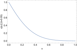
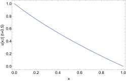
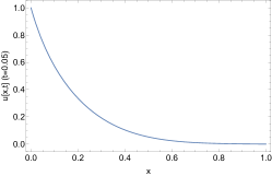
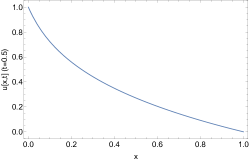
The figure illustrates distinct asymptotic behaviour for the two values of $a$ used. Assuming $k=r=1$, the two-point boundary value problem describing the long-run behaviour is then

$$u^{\prime\prime}+\frac{2a}{ax+b}u^{\prime}+u(1-u)=0$$ (16)

$$u(0)=1\quad u(1)=0.$$

This problem is not solvable by classical means, however the equations arising from linearization at the endpoints are both solvable in closed form. Suppose $u\approx 1$ and we replace the left-hand boundary condition with boundary conditions $u(0)=1$ and $u^{\prime}(0)=r_{0}<0$. The resulting linearized problem

$$u^{\prime\prime}+\frac{2a}{ax+b}u^{\prime}+(1-u)=0$$

$$u(0)=1\quad u^{\prime}(0)=r_{L}.$$

has closed form solution

$$u_{L}(x;r_{L})=\frac{br_{L}\sinh(x)}{ax+b}+1.$$

The corresponding right-hand-side problem is given by

$$u^{\prime\prime}+\frac{2a}{ax+b}u^{\prime}+u=0$$

$$u(1)=0\quad u^{\prime}(1)=r_{R},$$

with solution

$$u_{R}(x;r_{R})=-\frac{r_{R}(a+b)\sin(1-x)}{ax+b}.$$

As before, we know that $r_{R}\leq 0$. Surprisingly, these solutions can be combined to construct an approximation for the solution of Eq. 16, allowing us to explore the dynamics of the solutions. Let

$$\hat{u}(x;q,r_{L},r_{R})=\begin{cases}u_{L}(x;r_{L})&\text{if $x\in[0,q)$}\\ u_{R}(x;r_{R})&\text{if $x\in[q,1]$}.\end{cases}$$

The point $q$ and values for $r_{L}$ and $r_{R}$ are not known and must be approximated for each input $(a,b)$. We illustrate this in Fig. 3.

Figure 3: A comparison of $\hat{u}$ and $u$ showing goodness of fit of the approximate solution. The computed parameters are $q=0.413$, $r_{L}=-1.878$ and $r_{R}=-0.556$.

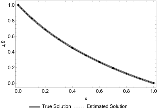
Assume we are given (a numerical solution for) $u(x)$. From this we can compute $u^{\prime}(0)=r_{L}$ and $u^{\prime}(1)=r_{R}$. It is easy to compute $q$ by solving the following optimization problem,

$$\arg\min_{q\in[0,1]}\;\;\int_{0}^{1}\left[u(x)-\hat{u}(x;q,r_{L},r_{R})\right]^{2}\,dx,$$ (17)

which can be accomplished using a simple dichotomous or golden section search [17]. Unfortunately, this still requires a numerical solution for $u(x)$ to determine $r_{L}$ and $r_{R}$. We can construct functions $r_{L}(a,b)$, $r_{R}(a,b)$ and $q(a,b)$ using a standard ordinary least squares approach. Without loss of generality, we fix $b=1$ and show the resulting analysis by varying $a$ only. We use the following procedure:

1. Choose $a$ from a sample space $\mathcal{A}$ with $a\geq 0$.

2. Compute $u(x)$ using a numerical solver.

3. Compute $r_{L}=u^{\prime}(0)$ and $r_{R}=u^{\prime}(1)$ using the output of the numerical solver.

4. Compute $q$ using Eq. 17.

5. Store $(a,q,r_{L},r_{R})$ for fitting.

Following this procedure leads to the data shown in Fig. 4.

Figure 4: (Top) Data and corresponding fit for $q(a)$. (Center) Data and corresponding fit for $r_{L}(a)$. Despite the appearance of linearity, there is a slight curvature. (Bottom) Data and corresponding fit for fit of $r_{R}(a)$.

The data can be fit with the following functions,

$$\hat{q}(a) \sim\frac{1}{(a+\alpha)^{\beta}},$$ (18)

$$\hat{r}_{L}(a) \sim\alpha\cdot a^{\beta},\text{ and}$$ (19)

$$\quad r_{R}(a) \sim\frac{1}{\alpha\cdot a^{\beta}}.$$ (20)

Tables of fit values are given in the insets of Fig. 4. The adjusted $r^{2}$ value for all three fits is $\sim 0.9999$, suggesting a high degree of accuracy in the underlying model. Consequently, when $b=1$ an approximate solution to Eq. 16 is given in closed form by

$$\hat{u}(x;a)\approx\begin{cases}\frac{\sinh(x)\left(-1.03a^{0.996}\right)}{ax+1}+1&0\leq x<\frac{1}{(a+3.29)^{0.621}}\\ -\frac{(a+1)\sin(1-x)\left(-0.883a^{0.993}\right)}{ax+1}&\frac{1}{(a+3.29)^{0.621}}\leq x<1\end{cases}$$

Fig. 5 shows anecdotal evidence for the goodness of fit of this approximation for larger values of $a$.

Figure 5: (Left) The approximation $\hat{u}$ and $u$ for $a=10$ shows a reasonable fit with a minor discontinuity. (Right) The approximation $\hat{u}$ and $u$ for $a=100$ showing very good fit.

We compute the maximum error

$$E_{\text{max}}=\max_{x}\left\lvert u(x;a)-\hat{u}(x;a)\right\rvert$$

for $a\in[0,1000]$. This is shown in Fig. 6.

Figure 6: The maximum error $E_{\text{max}}$ shows a rapid drop-off as $a$ increases. At $a=40$, the error is well below $0.005$, where it remains.

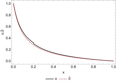
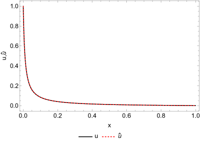
The figure shows that for $a>40$, the maximum approximation error is well below $0.005$, where it remains as $a$ increases. When combined with the ansatz from Section IV.1, we can formulate the following conjecture (to be proved as future work).

Conjecture 1.

Consider Eq. 16. As $a\to\infty$, the solution $u$ approaches the weak solution

$$u(x)=\begin{cases}1&\text{if x = 0}\\ 0&\text{if $0<x\leq 1$}.\end{cases}$$

Interestingly, this behaviour is consistent with the behaviour observed in the travelling wave solution. As $a\to\infty$, the population at $x=1$ becomes infinite. This is where $u(x)=0$ . As the system comes to equilibrium, the infinite population overwhelms the finite population of invaders at $x=0$, leading to the proposed weak solution. If we reversed the direction of population increase so that (e.g.) $M(x)=(a+1)-ax$ and let $a\to\infty$, we would see a limiting population with $u(x)=1$ for $0\leq x<1$ and $u(1)=0$.

IV.2 Neumann Boundary Conditions

It is worth briefly discussing Eq. 16 when the Dirichlet boundary conditions are replaced with Neumann boundary conditions.

$$\left\{\begin{aligned} &\frac{\partial u}{\partial t}=ru(1-u)+\frac{2ak}{ax+b}\frac{\partial u}{\partial x}+k\frac{\partial^{2}u}{\partial x^{2}}\\ &u_{x}(0)=0\quad u_{x}(1)=0.\\ &u(x,0)=u_{0}(x),\end{aligned}\right.$$ (21)

The long-run behaviour of this system is relatively easy to predict.

Conjecture 2.

Let $u(x,t)$ be a solution to Eq. 21 with $u_{0}(x)>0$ for some $x$. Then

$$\lim_{t\to\infty}u(x,t)=1.$$

This conjecture is supported by numerical analysis. Fix $\epsilon>0$ and let

$$u_{0}(x)=\begin{cases}1&\text{if $x<\epsilon$}\\ 0&\text{otherwise}.\end{cases}$$

This initial condition is consistent with the Neumann boundary conditions. Fig. 7 shows an early transient where $u(x,t)$ drops close to $0$ before the invasive species slowly takes over the entire population.

Figure 7: The time evolution of $u(x,t)$ for $t=0.005$ (left), $t=0.495$ (middle) and $t=7.495$ (right). This supports the conjecture that $\lim_{t\to\infty}u(x,t)=1$.

These dynamics are more consistent with the physical intuition associated with an invasive dominant species.

V Conclusion

In this paper, we studied the finite population Fisher-KPP equation, which arises naturally from the finite population spatial replicator using a skew-symmetric $2\times 2$ matrix. We showed using the results of Ablowitz and Zeppetella that this system of equations admits travelling wave solutions and showed a closed form solution that is identical to that in [13] except that the sign of the wave speed is reversed. We then studied the equilibrium problem for the finite population Fisher-KPP on a finite interval. We constructed a closed form approximate solution to this problem and used it to present a simple conjecture on the behaviour of populations with large spatial gradients.

There are several future directions that could be explored using the proposed finite population Fisher-KPP equation as a basis. For the purpose of this paper, we chose the travelling wave solution to the diffusion equation as the population equation. However, several closed form solutions to the diffusion equation exist and could be used, resulting in a new quasilinear reaction diffusion equation with a convection-like term. Also, in [14] it is noted there are no sensible stable amplitude travelling wave solutions when the logistic term $u(1-u)$ is replaced by a rock-paper-scissors dynamic, which arises from a $3\times 3$ skew-symmetric payoff matrices. This paper shows that $2\times 2$ skew-symmetric payoff matrices do give rise to travelling wave solutions in the finite population model. Therefore, it would be interesting to know whether any travelling wave solutions exist for $n\times n$ skew-symmetric payoff matrices with $n>3$ or if this is purely a property of $2\times 2$ payoff matrices. Proving the conjectures provided in this note are clearly a future direction of work with respect to the finite population Fisher-KPP equation in finite regions. However, an even more interesting direction might be to consider the problem on two-dimensional bounded regions (e.g., disks), where well known solutions to the Laplace equation are available. Studying more exotic boundary conditions (especially in two-dimensions) might also yield interesting results.

References

- Fisher [1937] R. A. Fisher, The wave of advance of advantageous genes, Annals of eugenics 7, 355 (1937).
- Kolmogorov et al. [1937] A. Kolmogorov, I. Petrovskii, and N. Piskunov, A study of the diffusion equation with increase in the amount of substance, and its application to a biological problem in selected works of an kolmogorov, vol. 1, 242-270, Bull. Moscow Univ., Math. Mech. 1, 1 (1937).
- Kenkre [2004] V. Kenkre, Results from variants of the fisher equation in the study of epidemics and bacteria, Physica A: Statistical Mechanics and its Applications 342, 242 (2004).
- Sardar et al. [2015] T. Sardar, S. Rana, and J. Chattopadhyay, A mathematical model of dengue transmission with memory, Communications in Nonlinear Science and Numerical Simulation 22, 511 (2015).
- Beneduci et al. [2021] R. Beneduci, E. Bilotta, and P. Pantano, A unifying nonlinear probabilistic epidemic model in space and time, Scientific Reports 11, 1 (2021).
- Mehmet [2012] M. Mehmet, Solutions of time-fractional reaction-diffusion equation with modified riemann-liouville derivative, International Journal of Physical Sciences 7, 2317 (2012).
- Neubert and Parker [2004] M. G. Neubert and I. M. Parker, Projecting rates of spread for invasive species, Risk Analysis: An International Journal 24, 817 (2004).
- Zel’Dovich and Raizer [2002] Y. B. Zel’Dovich and Y. P. Raizer, Physics of shock waves and high-temperature hydrodynamic phenomena (Courier Corporation, 2002).
- Kametaka [1976] Y. Kametaka, On the nonlinear diffusion equation of kolmogorov-petrovskii-piskunov type, Osaka Journal of Mathematics 13, 11 (1976).
- Uchiyama [1977] K. Uchiyama, The behavior of solutions of the equation of kolmogorov-petrovsky-piskunov, Proceedings of the Japan Academy, Series A, Mathematical Sciences 53, 225 (1977).
- Newman [1980] W. I. Newman, Some exact solutions to a non-linear diffusion problem in population genetics and combustion, Journal of Theoretical Biology 85, 325 (1980).
- Weinberger [1982] H. F. Weinberger, Long-time behavior of a class of biological models, SIAM journal on Mathematical Analysis 13, 353 (1982).
- Ablowitz and Zeppetella [1979] M. J. Ablowitz and A. Zeppetella, Explicit solutions of fisher’s equation for a special wave speed, Bulletin of Mathematical Biology 41, 835 (1979).
- Griffin et al. [2021] C. Griffin, R. Mummah, and R. DeForest, A finite population destroys a traveling wave in spatial replicator dynamics, Chaos, Solitons & Fractals 146, 110847 (2021).
- Vickers [1991] G. Vickers, Spatial patterns and travelling waves in population genetics, Journal of Theoretical Biology 150, 329 (1991).
- Durrett and Levin [1994] R. Durrett and S. Levin, The Importance of Being Discrete (and Spatial), Theoretical Population Biology 46, 363 (1994).
- Bazaraa et al. [2013] M. S. Bazaraa, H. D. Sherali, and C. M. Shetty, Nonlinear programming: theory and algorithms (John Wiley & Sons, 2013).