Constraining flavoured leptoquarks with LHC and LFV

Abstract

We consider the framework of flavoured leptoquarks, in models with scalar or vector leptoquarks, and look for constraints to the parameter space of these models. Using primarily direct searches at the Large Hadron Collider (LHC) and precision processes that probe Lepton Flavour Violation (LFV), we present lower bounds for the masses of the leptoquarks in different flavoured scenarios. We classify the models according to the specific leptoquark, distinguished with respect to their couplings to charged leptons (lepton isolation, two-columned patterns), and in scenarios with specific hierarchies in the couplings (hierarchical, democratic and flipped).

I Introduction

The Standard Model (SM) of Particle Physics continues to successfully describe most observations. We know there must be Physics Beyond the Standard Model (BSM) due to e.g. neutrino masses, dark matter and the baryon asymmetry of the universe.

With the current experimental situation, it is not at all clear what type of BSM extension stands to be the correct description of nature. In recent years, to a great extent due to hints that Lepton Flavour Universality (LFU) might be violated - something which does not occur in the SM - there has been great theoretical interest in extensions including flavoured leptoquarks (LQs), a scenario that has been explored extensively in the literature e.g. [1, 2, 3, 4, 5, 6, 7, 8, 9, 10, 11, 12, 13].

In December 2022, LHCb which supersede the previous results [14], and the recent results for $R_{K}$ and $R_{K^{*}}$ are in agreement with the SM prediction.

We summarise the experimental results in Table 1.

Observable	Experiment
$R_{K_{[0.1,1.1]}}$	$0.994\;^{+0.090}_{-0.082}\;({\rm stat})\;^{+0.029}_{-0.027}\;({\rm syst})$ [2022] [15, 14]
$R_{{K^{*}}_{[0.1,1.1]}}$	$0.927\;^{+0.093}_{-0.087}\;({\rm stat})\;^{+0.036}_{-0.035}\;({\rm syst})$ [2022] [15, 14]
$R_{K_{[1.1,6]}}$	$0.949\;^{+0.042}_{-0.041}\;({\rm stat})\;^{+0.022}_{-0.022}\;({\rm syst})$ [2022] [15, 14]
$R_{{K^{*}}_{[1.1,6]}}$	$1.027\;^{+0.072}_{-0.068}\;({\rm stat})\;^{+0.027}_{-0.026}\;({\rm syst})$ [2022] [15, 14]
$R_{K^{*}}^{[0.045,1.1]}$	$0.66^{+0.11}_{-0.07}\pm 0.03$ [2021] [16]
$R_{K^{*}}^{[1.1,6.0]}$	$0.69^{+0.11}_{-0.07}\pm 0.05$ [2021] [16]
$R_{K^{\phantom{*}}}^{[1.1,6.0]}$	$0.846^{+0.042+0.013}_{-0.039-0.012}$ [2021] [17]

Table 1: A summary of experimental results for $R_{K}$ and $R_{K^{*}}$. Compare with the SM predictions $R_{K}=1.00\pm 0.01$, $R_{K^{*}}^{[0.045,1.1]}=0.906\pm 0.028$ [18], $R_{K^{*}}^{[1.1,6.0]}=1.00\pm 0.01$.

This affects the motivation for this type of extension. Nevertheless, models with Flavoured LQs remain interesting and provide a better global fit to flavour data than the SM, see [19] with fits using data before and after December 2022. [20] considers in detail the impact of the hadronic uncertainties. Another consideration is that CP violation can supress new physics in the branching rations, as pointed out previously in [21] and more recently in [22] - such that LFU may be violated even with $R_{K}$ and $R_{K^{*}}$ in agreement with their SM values.

Regardless of theoretical bias for flavoured LQs, given current experimental results, it is possible to constrain the parameter space of these models. Some bounds were obtained in [10] and, in a recent work [23], mass bounds were obtained for LQs coupling either just to electrons or just to muons, and democratically to quarks. This is done by analysing the dielectron and dimuon decay channels. In this work, we consider several flavoured leptoquark (LQ) scenarios with scalar or vector LQs, with 3 benchmarks of couplings to quarks. We use Lepton Flavor Violation (LFV) results to provide bounds on the mass of the LQs whenever they apply. We constrain the masses also with results from the Large Hadron Collider (LHC), analysing decay channels with charged leptons and also with neutrinos.

The layout of this paper is as follows. In Section II we review briefly the leptoquark models we will consider. In Section VI.1 we present the flavoured patterns. These are then constrained through experimental results in Section III. We conclude in Section VI.

II Leptoquark Models

We consider three classes of leptoquark models, which we label according to the existing convention as models with the $S_{3}$, $R_{2}$ (scalar) and $U_{1}$ (vector) LQs.

II.1 Scalar Leptoquarks

II.1.1 $S_{3}\sim(\bar{3},3,1/3)$

We start by considering the $S_{3}$ LQ, with SM assignments $(\bar{3},3,1/3)$. This corresponds to an $SU(2)$ triplet that has hypercharge $Y=1/3$. These SM assignments are appealing as it has tree-level couplings that can justify both $R_{K^{*}}^{exp}<R_{K^{*}}^{SM}$ and $R_{K^{*}}^{exp}<R_{K^{*}}^{SM}$. In models with $S_{3}$, the couplings are

$$\mathcal{L}_{S_{3}}=\lambda^{ij}_{L}\bar{Q}^{C}_{i}i\tau_{2}(\tau_{k}S^{k}_{3})L_{j}+h.c.\,.$$ (II.1)

In this, we have denoted the 3 Pauli matrices as $\tau_{k}$, and the different $SU(2)$ components of $S_{3}$ are likewise denoted with a superscript. The (Yukawa) couplings of $S_{3}$ to the fermions are stored in the matrix $\lambda_{L}$. If $S_{3}$ couples to quark-quark it can mediate too fast proton decay, so we implicitly assume they vanish or are sufficiently suppressed by some unspecified mechanism (such as the residual symmetries invoked in [24, 25]. It is conventional to rewrite the couplings to $SU(2)$ components of $S_{3}$ with superscripts that identify the respective charge, as follows:

$$\mathcal{L}_{S_{3}} =-\lambda^{ij}_{L}\bar{d^{C}_{L_{i}}}\nu_{L_{j}}S_{3}^{(1/3)}-\sqrt{2}\lambda_{L}^{ij}\bar{d^{C}_{L_{i}}}l_{L_{j}}S_{3}^{(4/3)}$$

$$+\sqrt{2}(V^{*}\lambda_{L})_{ij}\bar{u^{C}_{L_{i}}}\nu_{L_{j}}S_{3}^{(-2/3)}-(V^{*}\lambda_{L})_{ij}\bar{u^{C}_{L_{i}}}l_{L_{j}}S_{3}^{(1/3)}+h.c.\,.$$ (II.2)

II.1.2 $R_{2}\sim(3,2,7/6)$

We consider another scalar LQ, $R_{2}$. In this class of models, the leptoquark has SM assignments $(3,2,7/6)$. This corresponds to an $SU(2)$ doublet that has hypercharge $Y=7/6$. Comparing this class of models to those with $S_{3}$ at tree-level, $R_{2}$ leads to $R_{K^{*}}^{exp}>R_{K^{*}}^{SM}$. In models with $R_{2}$, the couplings are

$$\mathcal{L}_{R_{2}}=\lambda^{ij}_{R}\bar{Q}_{i}l_{R_{j}}R_{2}-\lambda^{ij}_{L}\bar{u}_{R_{i}}R_{2}i\tau_{2}L_{j}+h.c.,$$ (II.3)

In this case we have (Yukawa) couplings to fermions stored in matrices $\lambda_{L}$ and $\lambda_{R}$. Rewriting with superscripts that identify the respective charge, the terms are as follows

$$\mathcal{L}_{R_{2}} =(V\lambda_{R})_{ij}\bar{u}_{L_{i}}l_{R_{j}}R_{2}^{(5/3)}+(\lambda_{R})_{ij}\bar{d}_{L_{i}}l_{R_{j}}R_{2}^{(2/3)}$$ (II.4)

$$+(\lambda_{L})_{ij}\bar{u}_{R_{i}}\nu_{L_{j}}R_{2}^{(2/3)}-(\lambda_{L})_{ij}\bar{u}_{R_{i}}l_{L_{j}}R_{2}^{(5/3)}+h.c.\,.$$ (II.5)

For our analysis, we have considered the phenomenology of both $\lambda_{L}$ and $\lambda_{R}$. The decays involving both couplings have been listed in III.2.

II.2 Vector Leptoquarks

II.2.1 $U_{1}\sim(3,1,2/3)$

We consider also a class of models with vector LQ $U_{1}$. The SM assignments are $(3,1,2/3)$. This corresponds to an $SU(2)$ singlet. In models with $U_{1}$, the couplings are

$$\begin{aligned} \mathcal{L}_{U}=&-\frac{1}{2}\,U_{1\,\mu\nu}^{\dagger}\,U_{1}^{\mu\nu}+M_{U}^{2}\,U_{1\,\mu}^{\dagger}\,U_{1}^{\mu}-ig_{c}(1-\kappa_{c})\,U_{1\,\mu}^{\dagger}\,T^{a}\,U_{1\,\nu}\,G^{a\,\mu\nu}\\ &-i\frac{2}{3}g_{Y}(1-\kappa_{Y})\,U_{1\,\mu}^{\dagger}\,\,U_{1\,\nu}\,B^{\mu\nu}+(U_{1}^{\mu}J_{\mu}+\mathrm{h.c.})\,.\end{aligned}$$ (II.6)

Following existing conventions in the literature, the covariant derivatives $D_{\mu}=\partial_{\mu}-ig_{c}\,G_{\mu}^{a}T^{a}-i\frac{2}{3}g_{Y}B_{\mu}$ and $U_{1\,\mu\nu}=D_{\mu}U_{1\,\nu}-D_{\nu}U_{1\,\mu}$. $T^{a}$ are $SU(3)_{c}$ generators, appearing with the ($SU(3)_{c}$ gluons) $G_{\mu}^{a}$ ($a=1,\dots,8$). The ($U(1)_{Y}$) $B_{\mu}$ is the SM gauge boson associated with the hypercharge. They are matched with the respective gauge couplings $g_{c}$ and $g_{Y}$.

In this class of models, there are parameters which distinguish the origin of the vector leptoquark. $\kappa_{c}=\kappa_{Y}=0$ corresponds to the LQ arising from a gauge origin. This should not be the case if $U_{1}$ arises from strongly-coupled origins. We can write

$$J_{\mu}=\frac{g_{U}}{\sqrt{2}}\left[\lambda_{L}^{i\alpha}\,(\bar{q}_{L}^{\,i}\gamma_{\mu}\ell_{L}^{\alpha})+\lambda_{R}^{i\alpha}\,(\bar{d}_{R}^{\,i}\gamma_{\mu}e_{R}^{\alpha})\right]\,.$$ (II.7)

The $\lambda_{L}$ and $\lambda_{R}$ are couplings of the vector LQs to the fermions. We are working on the basis where down-type quarks and charged-leptons have diagonal mass matrices such that we write

$$q_{L}^{i}=\begin{pmatrix}V_{ji}^{*}\,u^{j}_{L}\\ d_{L}^{i}\end{pmatrix}\,,\qquad\qquad\ell_{L}^{i}=\begin{pmatrix}\nu^{i}_{L}\\ e_{L}^{i}\end{pmatrix}\,.$$ (II.8)

For the $U_{1}$ model, we have considered the phenomenology of only left-handed coupling $\lambda_{L}$. The decays involving $\lambda_{L}$ have been listed in III.3.

II.3 Three benchmarks scenarios

In order to obtain indicative mass bounds, we consider the relative strengths of the LQ to the various fermions. In this section, we show the general couplings for all three scenarios. The notation of $\lambda_{0}$ is generic and should be adapted depending on the specific LQ considered, e.g. in the $R_{2}$ model, we have both $\lambda_{L}$ and $\lambda_{R}$ couplings which are taken into account separately when we use them for the phenomenological analysis. Here, we have considered three benchmark scenarios, [12]

Hierarchical scenario

The first scenario we consider is the same as in [5] based on flavor models discussed in [2], where we have made the assumption that the hierarchy found in the masses and mixtures in the SM also exists in LQ couplings. This would naturally arise in classes of flavour models, including very simple models using the Froggatt-Nielsen mechanism [26] to explain the hierarchies of fermion masses. In the Frogatt-Nielsen mechanism, an additional (Abelian) symmetry distinguishes the generations of the fermions, forbidding renormalisable Yukawa couplings for the lighter generations. They are allowed at tree level but at a non-renormalizable level through the coupling to an additional scalar field that breaks this additional symmetry. Given that the lighter generations are charged under this symmetry in this scenario, the leptoquark couplings to these fermions are suppressed similarly to the Yukawa couplings. Therefore we consider:

$$\lambda_{d\ell}\ :\ \lambda_{s\ell}\ :\ \lambda_{b\ell}\quad\sim\quad\epsilon^{3}\dots\epsilon^{4}\ :\ \epsilon^{2}\ :\ 1$$ (II.9)

between the different quark generations, where $\epsilon\sim 0.2$ is of the order of the Wolfenstein parameter, i.e. the sine of the Cabibbo angle. Specifically, we implement

$$\lambda_{ql}\sim\lambda_{0}\begin{pmatrix}0&0&0\\ \epsilon^{2}&\epsilon^{2}&\epsilon^{2}\\ 1&1&1\end{pmatrix}\,.$$ (II.10)

Where, $\lambda_{ql}$ and $\lambda_{0}$ are generic nomenclature for the LQ couplings to quark and leptons. From the eq. (II.10) we can see the coupling is larger for the third generation quarks, therefore with this benchmark the leptoquark decays to $b$ quark and $t$ quark for the down-type and up-type cases respectively. We have placed vanishing entries for the first row, experimentally they need to be small enough to respect constraints on rare kaon decays. In cases where the LQ couples to both $\mu$ and $e$ with the same quark, $\mu\to e$ processes come into effect and strongly constrain the couplings, as will be discussed subsequently.

Democratic scenario

Lastly, we consider a scenario where the couplings to the second and third quark generations are of equal size:

$$\lambda_{ql}\sim\lambda_{0}\begin{pmatrix}0&0&0\\ 1&1&1\\ 1&1&1\end{pmatrix}\,.$$ (II.11)

We refer to this as the democratic scenario. In this case, because the coupling is equal for second and third-generation quarks, the LQ decays in equal fractions to second and third-generation quarks for both down and up-type cases.

Flipped scenario

The second scenario is the inverted hierarchical case, i.e.:

$$\lambda_{ql}\sim\lambda_{0}\begin{pmatrix}0&0&0\\ 1&1&1\\ \epsilon^{2}&\epsilon^{2}&\epsilon^{2}\end{pmatrix}\,.$$ (II.12)

We refer to this as the flipped scenario. This scenario is opposite to the hierarchical case and with this pattern the LQ dominantly decays to the $s$ quark for the down-type case and $c$ quark for the up-type case due to the larger coupling constant associated with it.

In all benchmarks we consider, the scalar or vector, the number of parameters is small. We use three for scalar LQs: the mass, the dominant couplings $\lambda_{b\,l}$ and $\lambda_{s\,l}$. For vector LQs we have these three and also the parameter $\kappa$. These parameters can be constrained from the measurements of the single- or pair-production cross-section, the corresponding branching fractions and the resonance width, together with the reconstruction of the mass peak.

III Testing Flavoured Leptoquarks

In order to place experimental bounds on these flavoured LQs we have to consider different processes and experimental searches. A clear example arises when comparing lepton flavour isolation patterns with the two flavour patterns, where the two flavour patterns can be strongly constrained by Lepton Flavour Violating processes such as $\mu\to e\gamma$ (for $e\mu$), and for LFV meson decays such as $B\to K\mu^{\pm}e^{\mp}$ (and other lepton generations).

To get mass bounds on the LQs we have studied LQ single and pair production in $pp$-collisions and LQss decaying to up and down type quarks and different leptons using available search results from the ATLAS and CMS experiments in recent years.

Single and Pair Leptoquark Production and its Decay

In this paper, we have considered two dominant mechanisms of leptoquark production at pp colliders. Firstly, the single production of LQs is associated with a lepton and the pair production of LQs.

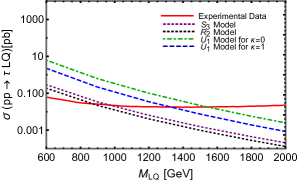
For the single production of LQ, we have considered the process $p\,p\to\tau lq$ corresponding to the coupling $\lambda_{L}$ for all three models because this is the best set of experimental data available [27] with our benchmarks for a single LQ production channel. Since for this type of process, the cross-section is directly proportional to the square of the magnitude of the coupling constant (at the parton level), our chosen three benchmarks very largely affect the production cross-sections which have been shown in the section IV.0.1.

Pair production of the LQs is primarily dominated by the strong interaction processes and it doesn’t depend on the flavour structure. The flavour structure is mainly responsible for determining the branching fractions into the final products. Based on our three flavour benchmarks (II.10), (II.12), (II.11) we can experimentally differentiate different patterns of the final products of the LQs in the two-body decays. We hereby list the dominant decays modes for $S_{3}$, $R_{2}$ and $U_{1}$ LQs [3][12],
For the $S_{3}$ model the decay modes are

$$S_{3}^{+2/3} \to t\ \nu_{l}\ ,\ c\ \nu_{l}$$

$$S_{3}^{-1/3} \to b\ \nu_{l}\ ,\ s\ \nu_{l}\ ,\ t\ l^{-}\ ,\ c\ l^{-}$$ (III.1)

$$S_{3}^{-4/3} \to b\ l^{-},\ s\ l^{-}$$

For the $R_{2}$ model the decay modes are

$$R_{2}^{+2/3} \to t\ \nu_{l}\ ,\ c\ \nu_{l}\ ,\ b\ l^{+}\ ,\ s\ l^{+}$$

$$R_{2}^{+5/3} \to \ t\ l^{+}\ ,\ c\ l^{+}$$ (III.2)

We note that $\lambda_{L}$ is responsible for the decay process $R_{2}^{+2/3}\to t\ \nu_{l}\ ,\ c\ \nu_{l}$ and $\lambda_{R}$ is responsible for the decay process $R_{2}^{+2/3}\to b\ l^{+}\ ,\ s\ l^{+}.$ For the process $R_{2}^{+5/3}\to\ t\ l^{+}\,\ c\ l^{+}$ both $\lambda_{L}$ and $\lambda_{R}$ are responsible but for our analysis, we have only considered the phenomenology due to the coupling $\lambda_{R}$ so that we can include the CKM induced effect to the up type quarks. This effect is important because the ATLAS experimental data, which we have used here, distinguish between light and heavy jets. Therefore, the phenomenology corresponding to the coupling $\lambda_{R}$ for this process is the only relevant one for the current sets of experimental data.

For the singlet $U_{1}$ leptoquark corresponding the coupling $\lambda_{L}$, the decay modes are

$$U_{1}^{+2/3}\to b\,l^{+}\,,\ t\,\bar{\nu}_{l}\,,\ s\,\ l^{+}\,,\ c\,\bar{\nu}_{l}$$ (III.3)

where $l$ represents the leptons of all generations.

IV Leptoquark Mass Bounds from LHC Searches

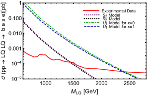
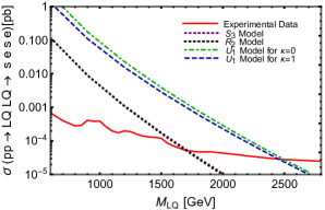
To evaluate the cross-sections of the different production and decay processes we use Madgraph5_amc@NLO to generate events [28]. The UFO model files we use here were implemented using Feynrules [29]. For the $S_{3}$ and $R_{2}$ models it has been described in [30] and for the $U_{1}$ model, it is described in [31][32][33]. The Lagrangian for each model, which has been described in II.1, II.3 and II.6 is implemented in Feynrules. As our main objective is to obtain the mass limits using various cuts provided in the literature, we haven’t included any uncertainties or detector simulations here. In the following sections, we present the plots of cross-sections (Y-axis) versus LQ mass (X-axis). For each process, we find an intersection point with the experimental line and thus obtain the respective mass bound for our benchmarks. In some cases where data was insufficient, we extrapolated the experimental data. For convenience, the mass bounds obtained are shown also in Tables. As we run the processes directly by putting the relevant decay states from the LQs based on our benchmarks in the Madgraph5_amc@NLO, we didn’t have to multiply the branching fractions with the cross-sections.

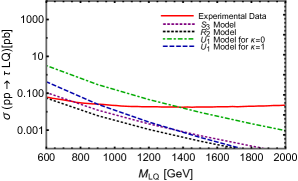
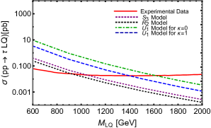
We have done three types of analysis, firstly single production of LQs where we run the process $pp\to\tau LQ$ and we got values of cross-sections for different masses of the LQs. We then used the data from $137fb^{-1}$, 13 TeV pp collisions[27] to find the intersection point for our theory runs. In section IV.0.1 we have put the plots and table for this run. Here, we discussed the process for scalar LQ models $S_{3}$ and $R_{2}$ and vector LQ models $U_{1}$ with $\kappa=$ 0 and $\kappa=$ 1 corresponding to the $\lambda_{L}$ coupling only, for all three benchmarks we mentioned before.

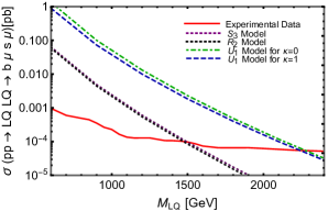
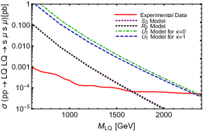
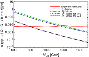
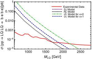
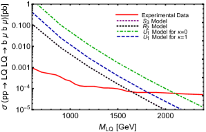
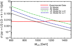
Secondly, we discuss the pair-produced LQs from pp collisions decaying into down (up) type quarks and leptons of all generations. For the down type quarks and leptons channel we have included $S_{3}$ and $R_{2}$ models and $U_{1}$ model with $\kappa=0$ and $\kappa=1$ corresponding to $S_{3}^{-4/3}$, $R_{2}^{+2/3}$ and $U_{1}^{+2/3}$ LQs respectively. In the down sector for the electrons and muons case we have used experimental data from 13 TeV ATLAS pp collisions data at 139 $fb^{-1}$[34] and for the tau lepton case we have used 13 TeV ATLAS 36.1 $fb^{-1}$ data [35]. For the tau lepton case, experimental data is available only for the $pp\to LQLQ\to b\tau b\tau$ channel, therefore we implemented our benchmarks to this channel only and we found out the bounds for the flipped ratio case was too weak. So, we have excluded the results for flipped ratio case here.

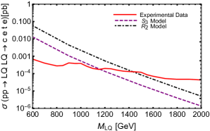
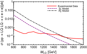
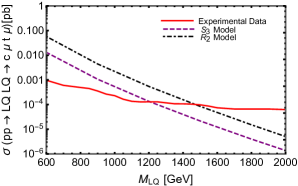
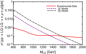
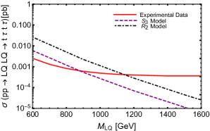
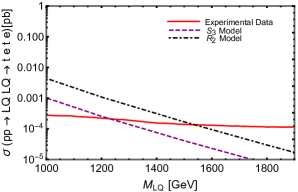
For the decays to up quarks and leptons, we have only analysed the $S_{3}$ and $R_{2}$ models corresponding to the $\lambda_{L}$ and $\lambda_{R}$ couplings ($S_{3}^{-1/3}$ and $R_{2}^{+5/3}$) respectively. In the $U_{1}$ model, we don’t get any decay final states to up quarks and leptons. In this section, we have included the CKM-induced effect on the up-type quarks to distinguish them from the light down-type quarks. This effect is also considered by the ATLAS experimental data to distinguish between light and heavy jets. For the values of the CKM matrix elements we have used the UTFIT Collaboration data from [36]. We have used experimental data from 13 TeV ATLAS pp collisions data at 139 $fb^{-1},$ [34] for charm quarks (for the democratic and flipped ratio) and the first two generations of leptons. For the top quark case (hierarchical) we have used recently published results from ATLAS data [37]. For the tau lepton case we had data available only for the $t\tau t\tau$ channel from the paper [38], therefore we used this data to obtain our mass bounds for our three benchmarks, although as it turned out the mass bound from the flipped case was very weak we didn’t include it here.

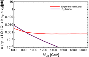
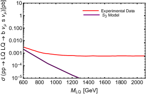
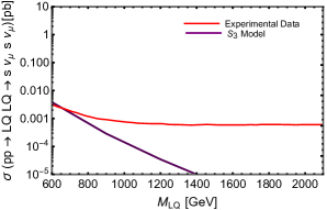
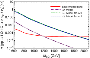
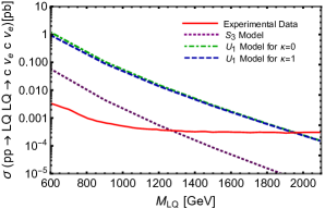
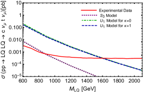
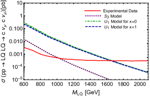
Lastly, we also looked into pair-produced LQs from pp collisions decaying into down (up) type quarks and neutrinos of the first two generations. We didn’t include the third generation of neutrinos because there was not enough experimental data available for this channel. As we can see from III only $S_{3}^{-1/3}$ can decay to down-type quarks and neutrinos, the rest all decay to up-type quarks and neutrinos. Therefore, we have first put the plots and tables of the process $pp\to S_{3}^{-1/3}S_{3}^{-1/3}\to qq\nu_{l}\nu_{l}$, ($l$ represents $e$ or $\mu$ and $q$ represents down-type quarks $b$ and $s$ quark here) in sections IV.0.8 and IV.0.9 for our benchmarks and then at sections IV.0.10 and IV.0.11 we have put the decays of $S_{3}^{2/3}$ and $U_{1}^{2/3}$ LQs ($U_{1}$ LQs for $\kappa=0$ and $\kappa=1$) which are decaying to up-type quarks and the neutrinos. For the $R_{2}$ model, we can see that this decay process is possible from the $\lambda_{L}$ coupling for the $R_{2}^{2/3}$ LQ, and ran the process in Madgraph, finding the mass-limits to be very low, and for this reason have not considered it further in this section. We first checked the mass bounds using [39] data from the $36.1fb^{-1}$ 2018 CMS paper but the bounds were stronger by considering the bounds with 13 TeV $139fb^{-1}$ ATLAS data[40], which was released very recently. As we obtained stronger bounds, We have used the ATLAS data for our analysis.

IV.0.1 Mass bounds from single production of LQs and tau leptons

Figure 1: Plot for the Cross-section (Y-axis) and LQ Mass(X-axis) for the process $pp\to\tau\,lq$ corresponding to the coupling $\lambda_{L}$ for all the models.  a) Upper Left Plot- Hierarchical Scenario   b) Upper Right Plot- Democratic Scenario   c) Lower Centre Plot- Flipped Scenario  The solid red line presents the experimental data from 13 TeV, 137 $fb^{-1}$ pp collisions [27]. The dotted purple and black line represent our theory results for $S_{3}$ and $R_{2}$ models respectively and the dashed blue and dot-dashed green line represent $U_{1}$ model results for $\kappa=1$ and $\kappa=0$ respectively.

Benchmark Case	$S_{3}$ model LQ Mass Limit(GeV)	$R_{2}$ model LQ Mass Limit(GeV)	$U_{1}$ model LQ Mass Limit(GeV) for $\kappa=0$	$U_{1}$ model LQ Mass Limit(GeV) for $\kappa=1$
Hierarchical	752	577	1375	1170
Democratic	1048	917	1612	1400
Flipped	972	872	1543	1327

Table 2: Bounds on the LQ mass from single production of LQs and tau leptons

IV.0.2 Mass Bounds of pair produced LQs decaying into down type quarks and electrons

Figure 2: Plot for the Cross-section (Y-axis) and LQ Mass(X-axis) for the process $pp\to lq\,lq\to qe^{+}qe^{-},$ where $q$ represents $b$ and $s$ quarks only. Here, the process is due to $\lambda_{L}$ coupling for the $S_{3}$ and $U_{1}$ models and $\lambda_{R}$ coupling for the $R_{2}$ model.  a) Upper Left Plot- Hierarchical Scenario   b) Upper Right Plot- Democratic Scenario   c) Lower Centre Plot- Flipped Scenario. The solid red line presents the experimental data from 13 TeV, 139 $fb^{-1}$ pp collisions [34]. We have used the $q\,e\,q\,e$ plot from the paper because we got better mass bounds. The dotted purple and black line represent our theory results for $S_{3}$ and $R_{2}$ models respectively and the dashed blue and dot-dashed green line represent $U_{1}$ model results for $\kappa=1$ and $\kappa=0$ respectively. We can see that the theory results for $S_{3}$ and $R_{2}$ models are very close and we can barely differentiate them. The decay states for each case are different based on the benchmark we have chosen. As we run the process directly in Madgraph, we don’t need to multiply the branching fractions with cross-sections. We can also see that the constant $\kappa$ for the $U_{1}$ model also affects the mass bounds of the LQs based on our benchmarks.

Benchmark Case	$S_{3}$ model LQ Mass Limit(GeV)	$R_{2}$ model LQ Mass Limit(GeV)	$U_{1}$ model LQ Mass Limit(GeV) for $\kappa=0$	$U_{1}$ model LQ Mass Limit(GeV) for $\kappa=1$
Hierarchical	1699	1695	2196	1877
Democratic	1455	1432	2420	2379
Flipped	1718	1700	2500	2453

Table 3: Bounds on the LQ mass for pair produced LQs decaying into down-type quarks and electrons.

IV.0.3 Mass Bounds of pair produced LQs decaying into down type quarks and muons

Figure 3: Plot for the Cross-section (Y-axis) and LQ Mass(X-axis) for the process $pp\to lq\,lq\to q\mu^{+}q\mu^{-},$ where $q$ represents $b$ and $s$ quarks only. Here, the process is due to $\lambda_{L}$ coupling for the $S_{3}$ and $U_{1}$ models and $\lambda_{R}$ coupling for the $R_{2}$ model.  a) Upper Left Plot- Hierarchical Scenario   b) Upper Right Plot- Democratic Scenario   c) Lower Centre Plot- Flipped Scenario. The solid red line presents the experimental data from 13 TeV, 139 $fb^{-1}$ pp collisions [34]. We have used the $q\,\mu\,q\,\mu$ plot here from the paper because we got better mass bounds. The dotted purple and black line represent our theory results for $S_{3}$ and $R_{2}$ models respectively and the dashed blue and dot-dashed green line represent $U_{1}$ model results for $\kappa=1$ and $\kappa=0$ respectively. We can see that the theory results for $S_{3}$ and $R_{2}$ models are very close and we can barely differentiate them. The decay states for each case are different based on the benchmark we have chosen. We can again see that the constant $\kappa$ for the $U_{1}$ model also affects the mass bounds of the LQs based on our benchmarks.

Benchmark Case	$S_{3}$ model LQ Mass Limit(GeV)	$R_{2}$ model LQ Mass Limit(GeV)	$U_{1}$ model LQ Mass Limit(GeV) for $\kappa=0$	$U_{1}$ model LQ Mass Limit(GeV) for $\kappa=1$
Hierarchical	1649	1646	2098	1816
Democratic	1497	1471	2279	2241
Flipped	1667	1649	2359	2315

Table 4: Bounds on the LQ mass for pair produced LQs decaying into down type quarks and muons.

IV.0.4 Mass Bounds of pair produced LQs decaying into down type quarks and tau leptons

Figure 4: Plot for the Cross-section (Y-axis) and LQ Mass(X-axis) for the process $pp\to lq\,lq\to b\tau^{+}b\tau^{-}$. Here again, the process is due to $\lambda_{L}$ coupling for the $S_{3}$ and $U_{1}$ models and $\lambda_{R}$ coupling for the $R_{2}$ model.  a) Upper Left Plot- Hierarchical Scenario   b) Upper Right Plot- Democratic Scenario.   The solid red line presents the experimental data from 13 TeV, 36.1 $fb^{-1}$ pp collisions [35]. We have used the $b\,\tau\,b\,\tau$ plot from the paper. The dotted purple and black line represent our theory results for $S_{3}$ and $R_{2}$ models respectively and the dashed blue and dot-dashed green line represent $U_{1}$ model results for $\kappa=1$ and $\kappa=0$ respectively. We can see here that the constant $\kappa$ for the $U_{1}$ model also affects the mass bounds of the LQs based on our benchmarks. Here, we haven’t plotted the results from flipped ratio scenario because the mass bounds were very weak due to small coupling to the bottom quark.

Benchmark Case	$S_{3}$ model LQ Mass Limit(GeV)	$R_{2}$ model LQ Mass Limit(GeV)	$U_{1}$ model LQ Mass Limit(GeV) for $\kappa=0$	$U_{1}$ model LQ Mass Limit(GeV) for $\kappa=1$
Hierarchical	981	982	1299	1106
Democratic	810	800	1186	1159

Table 5: Bounds on the LQ mass for pair produced LQs decaying into bottom quarks and tau leptons. The Flipped ratio benchmark hasn’t been placed here due to very weak limits.

IV.0.5 Mass Bounds of pair produced LQs decaying into up type quarks and electrons

Figure 5: Plot for the Cross-section (Y-axis) and LQ Mass(X-axis) for the process $pp\to lq\,lq\to qe^{+}qe^{-},$ where $q$ represents $c$ and $t$ quarks only. Here, the process is due to $\lambda_{L}$ coupling for the $S_{3}$ model and $\lambda_{R}$ coupling for the $R_{2}$ model.  a) Upper Left Plot- Hierarchical Scenario   b) Upper Right Plot- Democratic Scenario   c) Lower Centre Plot- Flipped Scenario. The solid red line presents the experimental data from 13 TeV, 139 $fb^{-1}$ pp collisions [34] and [37]. We have used the $q\,e\,q\,e$ plot from the paper [34] for the Democratic and Flipped case and $t\,e\,t\,e$ plot from [37] paper for the Hierarchical case due to better limits. The dashed purple and dot-dashed black lines represent our theory results for $S_{3}$ and $R_{2}$ models respectively. The decay states for each case are different based on the benchmark we have chosen. As we run the process directly in Madgraph, we don’t need to multiply the branching fractions with cross-sections.

Benchmark Case	$S_{3}$ model LQ Mass Limit(GeV)	$R_{2}$ model LQ Mass Limit(GeV)
Hierarchical	1231	1537
Democratic	1158	1432
Flipped	1238	1639

Table 6: Bounds on the LQ mass for pair produced LQs decaying into up-type quarks and electrons.

IV.0.6 Mass Bounds of pair produced LQs decaying into up type quarks and muons

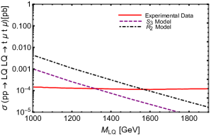
Figure 6: Plot for the Cross-section (Y-axis) and LQ Mass(X-axis) for the process $pp\to lq\,lq\to q\mu^{+}q\mu^{-},$ where $q$ represents $c$ and $t$ quarks only. Here, the process is due to $\lambda_{L}$ coupling for the $S_{3}$ model and $\lambda_{R}$ coupling for the $R_{2}$ model.  a) Upper Left Plot- Hierarchical Scenario   b) Upper Right Plot- Democratic Scenario   c) Lower Centre Plot- Flipped Scenario. The solid red line presents the experimental data from 13 TeV, 139 $fb^{-1}$ pp collisions [34] and [37]. We have used the $q\,\mu\,q\,\mu$ plot from the paper [34] for the Democratic and Flipped case and $t\,\mu\,t\,\mu$ plot from [37] for the Hierarchical case because of better limits. The dashed purple and dot-dashed black lines represent our theory results for $S_{3}$ and $R_{2}$ models respectively. The decay states for each case are different based on the benchmark we have chosen. As we run the process directly in Madgraph, we don’t need to multiply the branching fractions with cross-sections.

Benchmark Case	$S_{3}$ model LQ Mass Limit(GeV)	$R_{2}$ model LQ Mass Limit(GeV)
Hierarchical	1318	1568
Democratic	1207	1471
Flipped	1331	1587

Table 7: Bounds on the LQ mass for pair produced LQs decaying into up type quarks and muons.

IV.0.7 Mass Bounds of pair produced LQs decaying into up type quarks and tau leptons

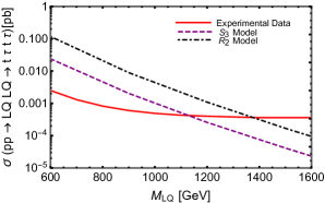
Figure 7: Plot for the Cross-section (Y-axis) and LQ Mass(X-axis) for the process $pp\to lq\,lq\to t\tau^{+}t\tau^{-}$.  Here, the process is due to $\lambda_{L}$ coupling for the $S_{3}$ model and $\lambda_{R}$ coupling for the $R_{2}$ model.  a) Upper Left Plot- Hierarchical Scenario   b) Upper Right Plot- Democratic Scenario.  The solid red line presents the experimental data from 13 TeV, 139 $fb^{-1}$ pp collisions [38]. We have used the $t\,\tau\,t\,\tau$ plot from the paper. The dashed purple and dot-dashed black lines represent our theory results for $S_{3}$ and $R_{2}$ models respectively. Here, we haven’t plotted the results from flipped ratio scenario because the mass bounds were very weak due to small coupling to the top quark.

Benchmark Case	$S_{3}$ model LQ Mass Limit(GeV)	$R_{2}$ model LQ Mass Limit(GeV)
Hierarchical	1128	1376
Democratic	877	1144

Table 8: Bounds on the LQ mass for pair produced LQs decaying into top quarks and tau leptons.

IV.0.8 Mass Bounds of pair produced LQs decaying into down type quarks and electron neutrinos

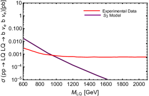
Figure 8: Plot for the Cross-section (Y-axis) and LQ Mass(X-axis) for the process $pp\to lq\,lq\to q\,\nu_{e}\,q\,\nu_{e},$ where $q$ represents $b$ and $s$ quarks only. Here, the process is due to $\lambda_{L}$ coupling for the $S_{3}$ model.  a) Upper Left Plot- Hierarchical Scenario   b) Upper Right Plot- Democratic Scenario   c) Lower Centre Plot- Flipped Scenario.  The solid red line presents the experimental data from 13 TeV, 139 $fb^{-1}$ pp collisions [40]. We have used the $q\,\nu_{e}\,q\,\nu_{e}$ plot from the paper for this analysis. The purple line represents our theory results for the $S_{3}$ model. The decay states for each case are different based on the benchmarks we have chosen. As we run the process directly in Madgraph, we don’t need to multiply the branching fractions with cross-sections.

Benchmark Case	$S_{3}$ model LQ Mass Limit(GeV)
Hierarchical	$952$
Democratic	$828$
Flipped	$939$

Table 9: Bounds on the LQ mass for pair produced LQs decaying into down-type quarks and electron neutrinos.

IV.0.9 Mass Bounds of pair produced LQs decaying into down type quarks and muon neutrinos

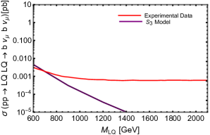
Figure 9: Plot for the Cross-section (Y-axis) and LQ Mass(X-axis) for the process $pp\to lq\,lq\to q\,\nu_{\mu}\,q\,\nu_{\mu},$ where $q$ represents $b$ and $s$ quarks only.   a) Upper Left Plot- Hierarchical Scenario   b) Upper Right Plot- Democratic Scenario   c) Lower Centre Plot- Flipped Scenario. The solid red line presents the experimental data from 13 TeV, 139 $fb^{-1}$ pp collisions [40]. We have used the $q\,\nu_{\mu}\,q\,\nu_{\mu}$ plot from the paper for this analysis. The purple line represents our theory results for the $S_{3}$ model. The decay states for each case are different based on the benchmarks we have chosen. As we run the process directly in Madgraph, we don’t need to multiply the branching fractions with cross-sections.

Benchmark Case	$S_{3}$ model LQ Mass Limit(GeV)
Hierarchical	$695$
Democratic	$580$
Flipped	$656$

Table 10: Bounds on the LQ mass for pair produced LQs decaying into down-type quarks and muon neutrinos.

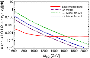
IV.0.10 Mass Bounds of pair produced LQs decaying into up type quarks and electron neutrinos

Figure 10: Plot for the Cross-section (Y-axis) and LQ Mass(X-axis) for the process $pp\to lq\,lq\to q\,\nu_{e}\,q\,\nu_{e},$ where $q$ represents $c$ and $t$ quarks only. For the $R_{2}$ model, we can see that this decay process is possible corresponding to $\lambda_{L}$ coupling, we, therefore, run the process in the Madgraph but we found that the mass-limits are well below $500$ GeV, therefore we haven’t plotted it here. a) Upper Left Plot- Hierarchical Scenario   b) Upper Right Plot- Democratic Scenario   c) Lower Centre Plot- Flipped Scenario.   The solid red line presents the experimental data from 13 TeV, 139 $fb^{-1}$ pp collisions [40]. We have used the $q\,\nu_{e}\,q\,\nu_{e}$ plot from the paper for this analysis. The dotted purple line represents our theory results for the $S_{3}$ model, and the dashed blue and dot-dashed green line represent our theory results for the $\kappa=1$ and $\kappa=0$ respectively. The decay states for each case are different based on the benchmarks we have chosen. As we run the process directly in Madgraph, we don’t need to multiply the branching fractions with cross-sections. We can again see that the constant $\kappa$ for the $U_{1}$ model also affects the mass bounds of the LQs based on our benchmarks.

Benchmark Case	$S_{3}$ model LQ Mass Limit(GeV)	$U_{1}$ model LQ Mass Limit(GeV) for $\kappa=0$	$U_{1}$ model LQ Mass Limit(GeV) for $\kappa=1$
Hierarchical	$1263$	$1665$	$1416$
Democratic	$1165$	$1920$	$1910$
Flipped	$1271$	$1957$	$1950$

Table 11: Bounds on the LQ mass for pair produced LQs decaying into up type quarks and electron neutrinos.

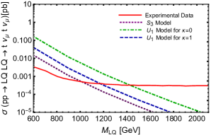
IV.0.11 Mass Bounds of pair produced LQs decaying into up type quarks and muon neutrinos

Figure 11: Plot for the Cross-section (Y-axis) and LQ Mass(X-axis) for the process $pp\to lq\,lq\to q\,\nu_{\mu}\,q\,\nu_{\mu},$ where $q$ represents $c$ and $t$ quarks only. Here, the process is due to $\lambda_{L}$ coupling for the $S_{3}$ and $U_{1}$ models.  For the $R_{2}$ model we can see that this decay process is possible corresponding to $\lambda_{L}$ coupling, we run the process in the Madgraph but we found that the mass-limits are well below $500$ GeV, therefore we haven’t plotted it here. a) Upper Left Plot- Hierarchical Scenario   b) Upper Right Plot- Democratic Scenario   c) Lower Centre Plot- Flipped Scenario   The solid red line presents the experimental data from 13 TeV, 139 $fb^{-1}$ pp collisions [40]. We have used the $q\,\nu_{\mu}\,q\,\nu_{\mu}$ plot from the paper for this analysis. The dotted purple line represents our theory results for the $S_{3}$ model, and the dashed blue and dot-dashed green line represent our theory results for the $\kappa=1$ and $\kappa=0$ respectively. The decay states for each case are different based on the benchmarks we have chosen. As we run the process directly in Madgraph, we don’t need to multiply the branching fractions with cross-sections. We can again see that the constant $\kappa$ for the $U_{1}$ model also affects the mass bounds of the LQs based on our benchmarks.

Benchmark Case	$S_{3}$ model LQ Mass Limit(GeV)	$U_{1}$ model LQ Mass Limit(GeV) for $\kappa=0$	$U_{1}$ model LQ Mass Limit(GeV) for $\kappa=1$
Hierarchical	$1013$	$1426$	$1172$
Democratic	$876$	$1608$	$1600$
Flipped	$1020$	$1663$	$1650$

Table 12: Bounds on the LQ mass for pair produced LQs decaying into up-type quarks and muon neutrinos.

V Mass bounds coming from Lepton Flavour Violating processes

In this section, we use the bounds from LFV processes presented in [1] to place bounds on LQs coupling to more than one lepton flavour. The expressions show the dependence on the specific couplings for each observable, and we use these to calculate the mass bounds for the Hierarchical, Flipped and Democratic scenarios. Note that strictly, these bounds strictly apply to the case of scalar LQs, as the computation of the processes differs for vector mediators.

Observable	Constraint	Hierarchical Scenario LQ Mass Limit (GeV)	Flipped Scenario LQ Mass Limit (GeV)	Democratic Scenario LQ Mass Limit (GeV)
${\cal{B}}(\mu\to e\gamma)$	$|\lambda_{qe}\lambda_{q\mu}^{*}|\lesssim\frac{M^{2}}{(34{\rm TeV})^{2}}$	$6800$	$6800$	$34000$
${\cal{B}}(\tau\to e\gamma)$	$|\lambda_{qe}\lambda_{q\tau}^{*}|\lesssim\frac{M^{2}}{(0.6{\rm TeV})^{2}}$	$120$	$120$	$600$
${\cal{B}}(\tau\to\mu\gamma)$	$|\lambda_{q\mu}\lambda_{q\tau}^{*}|\lesssim\frac{M^{2}}{(0.7\,{\rm TeV})^{2}}$	$140$	$140$	$700$
${\cal{B}}(B\to K\mu^{\pm}e^{\mp})$	$\sqrt{|\lambda_{s\mu}\lambda_{be}^{*}|^{2}+|\lambda_{b\mu}\lambda_{se}^{*}|^{2}}\lesssim\frac{M^{2}}{(19.4\,{\rm TeV})^{2}}$	$4614$	$4614$	$23070$
${\cal{B}}(B\to K\tau^{\pm}e^{\mp})$	$\sqrt{|\lambda_{s\tau}\lambda_{be}^{*}|^{2}+|\lambda_{b\tau}\lambda_{se}^{*}|^{2}}\lesssim\frac{M^{2}}{(3.3\,{\rm TeV})^{2}}$	$785$	$785$	$3925$
${\cal{B}}(B\to K\mu^{\pm}\tau^{\mp})$	$\sqrt{|\lambda_{s\mu}\lambda_{b\tau}^{*}|^{2}+|\lambda_{b\mu}\lambda_{s\tau}^{*}|^{2}}\lesssim\frac{M^{2}}{(2.9\,{\rm TeV})^{2}}$	$690$	$690$	$3450$

Table 13: Bounds on the LQ couplings from LFV processes ($q=d,s,b$). As in [1], we ignored tuning between leading order diagrams in the amplitudes of $\ell\to\ell^{\prime}\gamma$.

Figure 12: Top Left- Plot for the LQ Mass (Y-axis) and LQ Coupling(X-axis) for the process $\mu\to e\,\gamma$,   Top Right - Plot for the LQ Mass (Y-axis) and LQ Coupling(X-axis) for the process of $B\to K\,\mu\,e$   Bottom Left- Plot for the LQ Mass (Y-axis) and LQ Coupling(X-axis) for the process of $B\to K\,\tau\,e$   Bottom Right- Plot for the LQ Mass (Y-axis) and LQ Coupling(X-axis) for the process of $B\to K\,\mu\,\tau$. In this plot we want to show how the mass limits change based on the coupling constants for the LFV constraint for different decay processes. We haven’t plotted the other two channels from the table because the bounds are too low.

V.1 Summary of the results

We now summarise the results from the previous subsections. We first note that, for scalar LQs coupling to more than one lepton flavour, we have strict bounds from Lepton Flavor Violating processes. It is clear from the constraints that these are more stringent in the Democratic Scenario, in which case the mass of the LQ needs to be larger than 34 TeV if it couples to both of the lighter generations of charged leptons ($e\mu$). For Democratic Scenarios coupling to $\tau$ and one of the lighter-charged leptons, the mass bound is still above 3 TeV. The Hierarchical and Flipped Scenarios have considerably weaker bounds by about one order of magnitude, as seen in Table 13.

With respect to constraints coming from the LHC, Democratic Scenarios are bounded roughly at the order of 1 to 1.5 TeV (depending on whether $S_{3}$, $R_{2}$, $U_{1}$ ($\kappa=0$, $\kappa=1$). A few stronger bounds are obtained with e.g. vector LQs coupling to muons, with mass excluded below 2 TeV, and vector LQs coupling to electrons, with mass excluded below 2.5 TeV in some cases.

We note that the mass bounds obtained from decay channels involving neutrinos are always weaker than the corresponding bounds using other decay channels.

VI Conclusions

We have considered a Beyond the SM framework where we add either scalar or vector LQs. We classify the flavour couplings of the LQ to the SM fermions according to the leptons that do or do not couple to the LQ. These scenarios are motivated by underlying flavour symmetries that can force couplings to vanish.

For each class of LQs, we investigate the processes that lead to the strongest bounds on the LQ mass.

Apart from the expectation associated with lepton flavour violation bounds coming from $\mu$ to $e$ processes that have very high precision, the mass bounds obtained are of the order of a few TeV. The detailed bounds depend on the type of LQ, the leptons it couples to, and the specific scenario (if the couplings are democratic or hierarchical). We have systematically presented bounds for each of these options, providing a comprehensive approach that highlights the present constraints on flavoured LQ models.

Appendix

VI.1 Leptoquark flavoured patterns

We briefly review here the type of LQ couplings we are considering. We have shown the most generalised couplings for all three models and the notation should differ for different models when it is implemented in the theory and for phenomenological analysis. We note that these specific patterns can be obtained by the same type of flavour symmetries that are used to address the flavour problem of the SM [1].

We take 3 lepton isolation patterns, where the LQ couples only to electron or to muon or to tau, and 3 two-columned patterns where the LQ does not couple to electron or to muon or to tau:

$$\lambda^{[e]}_{dl}=\left(\begin{array}[]{ccc}\lambda_{de}&0&0\\ \lambda_{se}&0&0\\ \lambda_{be}&0&0\end{array}\right),\,\,\,\,\,\lambda^{[\mu]}_{dl}=\left(\begin{array}[]{ccc}0&\lambda_{d\mu}&0\\ 0&\lambda_{s\mu}&0\\ 0&\lambda_{b\mu}&0\end{array}\right),\,\,\,\,\,\lambda^{[\tau]}_{dl}=\left(\begin{array}[]{ccc}0&0&\lambda_{d\tau}\\ 0&0&\lambda_{s\tau}\\ 0&0&\lambda_{b\tau}\end{array}\right)\,,$$ (VI.1)

We obtain the couplings to e.g. up-type quarks by proceeding as described in [24]. The coupling to up type quarks corresponding to $\lambda^{[e]}_{dl}$ (with $\lambda_{de}=0$):

$$\lambda^{[e]}_{ul}=\frac{1}{\sqrt{2}}\left(\begin{array}[]{ccc}V_{ub}\lambda_{be}+V_{us}\lambda_{se}&0&0\\ V_{cb}\lambda_{be}+V_{cs}\lambda_{se}&0&0\\ V_{tb}\lambda_{be}+V_{ts}\lambda_{se}&0&0\end{array}\right)\,.$$ (VI.2)

The other isolation cases have corresponding

$$\lambda^{[\mu]}_{ul}=\frac{1}{\sqrt{2}}\left(\begin{array}[]{ccc}0&V_{ub}\lambda_{b\mu}+V_{us}\lambda_{s\mu}&0\\ 0&V_{cb}\lambda_{b\mu}+V_{cs}\lambda_{s\mu}&0\\ 0&V_{tb}\lambda_{b\mu}+V_{ts}\lambda_{s\mu}&0\end{array}\right),\,\,\,\,\,\,\,\,\,\,\lambda^{[\tau]}_{ul}=\frac{1}{\sqrt{2}}\left(\begin{array}[]{ccc}0&0&V_{ub}\lambda_{b\tau}+V_{us}\lambda_{s\tau}\\ 0&0&V_{cb}\lambda_{b\tau}+V_{cs}\lambda_{s\tau}\\ 0&0&V_{tb}\lambda_{b\tau}+V_{ts}\lambda_{s\tau}\end{array}\right)\,.$$ (VI.3)

For the up-type quark and charged-lepton couplings $\lambda_{ul}$, rigorously the coupling matrices respective to each of the down-type couplings should be used. We use simplified structures by putting the first row to zero and checked that the difference in terms of the LQ mass bounds with respect to the rigorous structure was negligible (1 part in 10000).
For a lepton isolation case for neutrinos such as electron isolation (with $\lambda_{de}=0$), the corresponding $\lambda_{d\nu}$ is:

$$\lambda_{d\nu}^{[e]}=\frac{1}{\sqrt{2}}\left(\begin{array}[]{ccc}0&0&0\\ U_{11}\lambda_{se}&U_{12}\lambda_{se}&U_{13}\lambda_{se}\\ U_{11}\lambda_{be}&U_{12}\lambda_{be}&U_{13}\lambda_{be}\end{array}\right)$$ (VI.4)

Where $U$ is the PMNS matrix. The other isolation cases have corresponding

$$\lambda_{d\nu}^{[\mu]}=\frac{1}{\sqrt{2}}\left(\begin{array}[]{ccc}0&0&0\\ U_{21}\lambda_{s\mu}&U_{22}\lambda_{s\mu}&U_{23}\lambda_{s\mu}\\ U_{21}\lambda_{b\mu}&U_{22}\lambda_{b\mu}&U_{23}\lambda_{b\mu}\end{array}\right),\,\,\,\,\,\,\,\,\,\,\lambda_{d\nu}^{[\tau]}=\frac{1}{\sqrt{2}}\left(\begin{array}[]{ccc}0&0&0\\ U_{31}\lambda_{s\tau}&U_{32}\lambda_{s\tau}&U_{33}\lambda_{s\tau}\\ U_{31}\lambda_{b\tau}&U_{32}\lambda_{b\tau}&U_{33}\lambda_{b\tau}\end{array}\right)\,.$$ (VI.5)

For the couplings to up-type quarks case one obtains for $\lambda_{dl}^{[e]}$ (with $\lambda_{de}=0$),

$$\lambda_{u\nu}^{[e]}=\left(\begin{array}[]{ccc}U_{11}\left(V^{\star}_{ub}\lambda_{be}+V^{\star}_{us}\lambda_{se}\right)&U_{12}\left(V^{\star}_{ub}\lambda_{be}+V^{\star}_{us}\lambda_{se}\right)&U_{13}\left(V^{\star}_{ub}\lambda_{be}+V^{\star}_{us}\lambda_{se}\right)\\ U_{11}\left(V^{\star}_{cb}\lambda_{be}+V^{\star}_{cs}\lambda_{se}\right)&U_{12}\left(V^{\star}_{cb}\lambda_{be}+V^{\star}_{cs}\lambda_{se}\right)&U_{13}\left(V^{\star}_{cb}\lambda_{be}+V^{\star}_{cs}\lambda_{se}\right)\\ U_{11}\left(V^{\star}_{tb}\lambda_{be}+V^{\star}_{ts}\lambda_{se}\right)&U_{12}\left(V^{\star}_{tb}\lambda_{be}+V^{\star}_{ts}\lambda_{se}\right)&U_{13}\left(V^{\star}_{tb}\lambda_{be}+V^{\star}_{ts}\lambda_{se}\right)\end{array}\right)\,.$$ (VI.6)

For $\lambda_{dl}^{[\mu]}$,

$$\lambda_{u\nu}^{[\mu]}=\left(\begin{array}[]{ccc}U_{21}\left(V^{\star}_{ub}\lambda_{b\mu}+V^{\star}_{us}\lambda_{s\mu}\right)&U_{22}\left(V^{\star}_{ub}\lambda_{b\mu}+V^{\star}_{us}\lambda_{s\mu}\right)&U_{23}\left(V^{\star}_{ub}\lambda_{b\mu}+V^{\star}_{us}\lambda_{s\mu}\right)\\ U_{21}\left(V^{\star}_{cb}\lambda_{b\mu}+V^{\star}_{cs}\lambda_{s\mu}\right)&U_{22}\left(V^{\star}_{cb}\lambda_{b\mu}+V^{\star}_{cs}\lambda_{s\mu}\right)&U_{23}\left(V^{\star}_{cb}\lambda_{b\mu}+V^{\star}_{cs}\lambda_{s\mu}\right)\\ U_{21}\left(V^{\star}_{tb}\lambda_{b\mu}+V^{\star}_{ts}\lambda_{s\mu}\right)&U_{22}\left(V^{\star}_{tb}\lambda_{b\mu}+V^{\star}_{ts}\lambda_{s\mu}\right)&U_{23}\left(V^{\star}_{tb}\lambda_{b\mu}+V^{\star}_{ts}\lambda_{s\mu}\right)\end{array}\right)\,.$$ (VI.7)

For $\lambda_{dl}^{[\tau]}$,

$$\lambda_{u\nu}^{[\tau]}=\left(\begin{array}[]{ccc}U_{31}\left(V^{\star}_{ub}\lambda_{b\tau}+V^{\star}_{us}\lambda_{s\tau}\right)&U_{32}\left(V^{\star}_{ub}\lambda_{b\tau}+V^{\star}_{us}\lambda_{s\tau}\right)&U_{33}\left(V^{\star}_{ub}\lambda_{b\tau}+V^{\star}_{us}\lambda_{s\tau}\right)\\ U_{31}\left(V^{\star}_{cb}\lambda_{b\tau}+V^{\star}_{cs}\lambda_{s\tau}\right)&U_{32}\left(V^{\star}_{cb}\lambda_{b\tau}+V^{\star}_{cs}\lambda_{s\tau}\right)&U_{33}\left(V^{\star}_{cb}\lambda_{b\tau}+V^{\star}_{cs}\lambda_{s\tau}\right)\\ U_{31}\left(V^{\star}_{tb}\lambda_{b\tau}+V^{\star}_{ts}\lambda_{s\tau}\right)&U_{32}\left(V^{\star}_{tb}\lambda_{b\tau}+V^{\star}_{ts}\lambda_{s\tau}\right)&U_{33}\left(V^{\star}_{tb}\lambda_{b\tau}+V^{\star}_{ts}\lambda_{s\tau}\right)\end{array}\right)\,.$$ (VI.8)

References

• [1] I. de Medeiros Varzielas and G. Hiller, Clues for flavor from rare lepton and quark decays, JHEP 06 (2015) 072 [1503.01084].
• [2] G. Hiller, D. Loose and K. Schönwald, Leptoquark Flavor Patterns & B Decay Anomalies, JHEP 12 (2016) 027 [1609.08895].
• [3] G. Hiller and I. Nisandzic, RKsubscript𝑅𝐾R_{K} and RKsubscript𝑅superscript𝐾R_{K^{\ast}} beyond the standard model, Phys. Rev. D 96 (2017) 035003 [1704.05444].
• [4] L. Calibbi, A. Crivellin and T. Li, Model of vector leptoquarks in view of the B𝐵B-physics anomalies, Phys. Rev. D 98 (2018) 115002 [1709.00692].
• [5] G. Hiller, D. Loose and I. Nišandžić, Flavorful leptoquarks at hadron colliders, Phys. Rev. D 97 (2018) 075004 [1801.09399].
• [6] I. de Medeiros Varzielas and S.F. King, RK()subscript𝑅superscript𝐾{R}_{K^{\left(*\right)}} with leptoquarks and the origin of Yukawa couplings, JHEP 11 (2018) 100 [1807.06023].
• [7] I. De Medeiros Varzielas and S.F. King, Origin of Yukawa couplings for Higgs bosons and leptoquarks, Phys. Rev. D 99 (2019) 095029 [1902.09266].
• [8] C. Cornella, J. Fuentes-Martin and G. Isidori, Revisiting the vector leptoquark explanation of the B-physics anomalies, JHEP 07 (2019) 168 [1903.11517].
• [9] J. Bernigaud, I. de Medeiros Varzielas and J. Talbert, Finite Family Groups for Fermionic and Leptoquark Mixing Patterns, JHEP 01 (2020) 194 [1906.11270].
• [10] K.S. Babu, P.S.B. Dev, S. Jana and A. Thapa, Unified framework for B𝐵B-anomalies, muon g2𝑔2g-2 and neutrino masses, JHEP 03 (2021) 179 [2009.01771].
• [11] A. Crivellin, C. Greub, D. Müller and F. Saturnino, Scalar Leptoquarks in Leptonic Processes, JHEP 02 (2021) 182 [2010.06593].
• [12] G. Hiller, D. Loose and I. Nišandžić, Flavorful leptoquarks at the LHC and beyond: spin 1, JHEP 06 (2021) 080 [2103.12724].
• [13] J. Bernigaud, M. Blanke, I. de Medeiros Varzielas, J. Talbert and J. Zurita, LHC signatures of τ𝜏\tau-flavoured vector leptoquarks, JHEP 08 (2022) 127 [2112.12129].
• [14] LHCb collaboration, Measurement of lepton universality parameters in B+K++superscript𝐵superscript𝐾superscriptsuperscriptB^{+}\to K^{+}\ell^{+}\ell^{-} and B0K0+superscript𝐵0superscript𝐾absent0superscriptsuperscriptB^{0}\to K^{*0}\ell^{+}\ell^{-} decays, 2212.09153.
• [15] LHCb collaboration, Test of lepton universality in bs+𝑏𝑠superscriptsuperscriptb\rightarrow s\ell^{+}\ell^{-} decays, 2212.09152.
• [16] LHCb collaboration, Test of lepton universality with B0K0+superscript𝐵0superscript𝐾absent0superscriptsuperscriptB^{0}\rightarrow K^{*0}\ell^{+}\ell^{-} decays, JHEP 08 (2017) 055 [1705.05802].
• [17] LHCb collaboration, Test of lepton universality in beauty-quark decays, Nature Phys. 18 (2022) 277 [2103.11769].
• [18] M. Bordone, G. Isidori and A. Pattori, On the Standard Model predictions for RKsubscript𝑅𝐾R_{K} and RKsubscript𝑅superscript𝐾R_{K^{*}}, Eur. Phys. J. C 76 (2016) 440 [1605.07633].
• [19] B. Allanach and J. Davighi, The Rumble in the Meson: a leptoquark versus a Zsuperscript𝑍Z^{\prime} to fit bsμ+μ𝑏𝑠superscript𝜇superscript𝜇b\rightarrow s\mu^{+}\mu^{-} anomalies including 2022 LHCb RK()subscript𝑅superscript𝐾R_{K^{(\ast)}} measurements, 2211.11766.
• [20] M. Ciuchini, M. Fedele, E. Franco, A. Paul, L. Silvestrini and M. Valli, Constraints on lepton universality violation from rare B decays, Phys. Rev. D 107 (2023) 055036 [2212.10516].
• [21] G. Hiller and M. Schmaltz, Diagnosing lepton-nonuniversality in bs𝑏𝑠b\to s\ell\ell, JHEP 02 (2015) 055 [1411.4773].
• [22] R. Fleischer, E. Malami, A. Rehult and K.K. Vos, New Perspectives for Testing Electron-Muon Universality, 2303.08764.
• [23] N. Desai and A. Sengupta, Status of leptoquark models after LHC Run-2 and discovery prospects at future colliders, 2301.01754.
• [24] I. de Medeiros Varzielas and J. Talbert, Simplified Models of Flavourful Leptoquarks, Eur. Phys. J. C 79 (2019) 536 [1901.10484].
• [25] J. Bernigaud, I. de Medeiros Varzielas and J. Talbert, Reconstructing Effective Lagrangians Embedding Residual Family Symmetries, Eur. Phys. J. C 81 (2021) 65 [2005.12293].
• [26] C.D. Froggatt and H.B. Nielsen, Hierarchy of Quark Masses, Cabibbo Angles and CP Violation, Nucl. Phys. B 147 (1979) 277.
• [27] CMS collaboration, Search for singly and pair-produced leptoquarks coupling to third-generation fermions in proton-proton collisions at s=13 TeV, Phys. Lett. B 819 (2021) 136446 [2012.04178].
• [28] J. Alwall, M. Herquet, F. Maltoni, O. Mattelaer and T. Stelzer, MadGraph 5 : Going Beyond, JHEP 06 (2011) 128 [1106.0522].
• [29] A. Alloul, N.D. Christensen, C. Degrande, C. Duhr and B. Fuks, FeynRules 2.0 - A complete toolbox for tree-level phenomenology, Comput. Phys. Commun. 185 (2014) 2250 [1310.1921].
• [30] I. Doršner and A. Greljo, Leptoquark toolbox for precision collider studies, JHEP 05 (2018) 126 [1801.07641].
• [31] M.J. Baker, J. Fuentes-Martín, G. Isidori and M. König, High- pTsubscript𝑝𝑇p_{T} signatures in vector–leptoquark models, Eur. Phys. J. C 79 (2019) 334 [1901.10480].
• [32] L. Di Luzio, J. Fuentes-Martin, A. Greljo, M. Nardecchia and S. Renner, Maximal Flavour Violation: a Cabibbo mechanism for leptoquarks, JHEP 11 (2018) 081 [1808.00942].
• [33] C. Cornella, D.A. Faroughy, J. Fuentes-Martin, G. Isidori and M. Neubert, Reading the footprints of the B-meson flavor anomalies, JHEP 08 (2021) 050 [2103.16558].
• [34] ATLAS collaboration, Search for pairs of scalar leptoquarks decaying into quarks and electrons or muons in s𝑠\sqrt{s} = 13 TeV pp𝑝𝑝pp collisions with the ATLAS detector, JHEP 10 (2020) 112 [2006.05872].
• [35] ATLAS collaboration, Searches for third-generation scalar leptoquarks in s𝑠\sqrt{s} = 13 TeV pp collisions with the ATLAS detector, JHEP 06 (2019) 144 [1902.08103].
• [36] UTfit collaboration, The Unitarity Triangle Fit in the Standard Model and Hadronic Parameters from Lattice QCD: A Reappraisal after the Measurements of Delta m(s) and BR(B —>> tau nu(tau)), JHEP 10 (2006) 081 [hep-ph/0606167].
• [37] ATLAS collaboration, Search for leptoquark pair production decaying to tlt¯l+𝑡superscript𝑙¯𝑡superscript𝑙tl^{-}\bar{t}l^{+} in multilepton final states in pp collisions at 13 TeV with the ATLAS detector, .
• [38] ATLAS collaboration, Search for pair production of third-generation scalar leptoquarks decaying into a top quark and a τ𝜏\tau-lepton in pp𝑝𝑝pp collisions at s𝑠\sqrt{s} = 13 TeV with the ATLAS detector, JHEP 06 (2021) 179 [2101.11582].
• [39] CMS collaboration, Constraints on models of scalar and vector leptoquarks decaying to a quark and a neutrino at s=𝑠absent\sqrt{s}= 13 TeV, Phys. Rev. D 98 (2018) 032005 [1805.10228].
• [40] ATLAS collaboration, Search for pair-produced scalar and vector leptoquarks decaying into third-generation quarks and first- or second-generation leptons in pp collisions with the ATLAS detector, 2210.04517.