L[1]Q[l,#1] C[1]Q[c,#1] R[1]Q[r,#1] mytabular[1]

Mastering Diverse Domains through World Models

Abstract

General intelligence requires solving tasks across many domains. Current reinforcement learning algorithms carry this potential but are held back by the resources and knowledge required to tune them for new tasks. We present DreamerV3, a general and scalable algorithm based on world models that outperforms previous approaches across a wide range of domains with fixed hyperparameters. These domains include continuous and discrete actions, visual and low-dimensional inputs, 2D and 3D worlds, different data budgets, reward frequencies, and reward scales. We observe favorable scaling properties of DreamerV3, with larger models directly translating to higher data-efficiency and final performance. Applied out of the box, DreamerV3 is the first algorithm to collect diamonds in Minecraft from scratch without human data or curricula, a long-standing challenge in artificial intelligence. Our general algorithm makes reinforcement learning broadly applicable and allows scaling to hard decision making problems.

Figure 1: Using the same hyperparameters across all domains, DreamerV3 outperforms specialized model-free and model-based algorithms in a wide range of benchmarks and data-efficiency regimes. Applied out of the box, DreamerV3 also learns to obtain diamonds in the popular video game Minecraft from scratch given sparse rewards, a long-standing challenge in artificial intelligence for which previous approaches required human data or domain-specific heuristics.

(a) Control Suite

(b) Atari

(c) DMLab

(d) Minecraft

Figure 2: Four visual domains considered in this work. DreamerV3 succeeds across these diverse domains, ranging from robot locomotion and manipulation tasks over Atari games with 2D graphics to complex 3D domains such as DMLab and Minecraft that require spatial and temporal reasoning.

Introduction

Reinforcement learning has enabled computers to solve individual tasks through interaction, such as surpassing humans in the games of Go and Dota ¹, ². However, applying algorithms to new application domains, for example from board games to video games or robotics tasks, requires expert knowledge and computational resources for tuning the algorithms ³. This brittleness also hinders scaling to large models that are expensive to tune. Different domains pose unique learning challenges that have prompted specialized algorithms, such as for continuous control ⁴, ⁵, sparse rewards ⁶, ⁷, image inputs ⁸, ⁹, and spatial environments ¹⁰, ¹¹. Creating a general algorithm that learns to master new domains out of the box—without tuning—would overcome the barrier of expert knowledge and open up reinforcement learning to a wide range of practical applications.

We present DreamerV3, a general and scalable algorithm that masters a wide range of domains with fixed hyperparameters, outperforming specialized algorithms. DreamerV3 learns a world model ¹², ¹³, ¹⁴ from experience for rich perception and imagination training. The algorithm consists of 3 neural networks: the world model predicts future outcomes of potential actions, the critic judges the value of each situation, and the actor learns to reach valuable situations. We enable learning across domains with fixed hyperparameters by transforming signal magnitudes and through robust normalization techniques. To provide practical guidelines for solving new challenges, we investigating the scaling behavior of DreamerV3. Notably, we demonstrate that increasing the model size of DreamerV3 monotonically improves both its final performance and data-efficiency.

The popular video game Minecraft has become a focal point of reinforcement learning research in recent years, with international competitions held for learning to collect diamonds in Minecraft ¹⁵. Solving this challenge without human data has been widely recognized as a milestone for artificial intelligence because of the sparse rewards, exploration difficulty, and long time horizons in this procedurally generated open-world environment. Due to these obstacles, previous approaches resorted to human expert data and manually-crafted curricula ¹⁶, ¹⁷. DreamerV3 is the first algorithm to collect diamonds in Minecraft from scratch, solving this challenge.

We summarize the four key contributions of this paper as follows:

• We present DreamerV3, a general algorithm that learns to master diverse domains while using fixed hyperparameters, making reinforcement learning readily applicable.

• We demonstrate the favorable scaling properties of DreamerV3, where increased model size leads to monotonic improvements in final performance and data-efficiency.

• We perform an extensive evaluation, showing that DreamerV3 outperforms more specialized algorithms across domains, and release the training curves of all methods to facilitate comparison.

• We find that DreamerV3 is the first algorithm to collect diamonds in Minecraft from scratch without human data or curricula, solving a long-standing challenge in artificial intelligence.

(a) World Model Learning

(b) Actor Critic Learning

Figure 3: Training process of DreamerV3. The world model encodes sensory inputs into a discrete representation $z_{t}$ that is predicted by a sequence model with recurrent state $h_{t}$ given actions $a_{t}$. The inputs are reconstructed as learning signal to shape the representations. The actor and critic learn from trajectories of abstract representations predicted by the world model.

DreamerV3

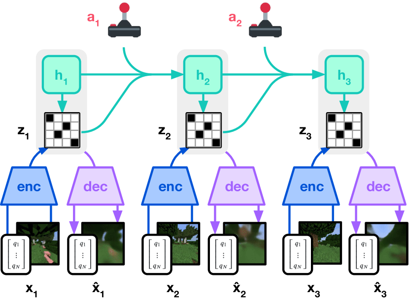
The DreamerV3 algorithm consists of 3 neural networks—the world model, the critic, and the actor—that are trained concurrently from replayed experience without sharing gradients, as shown in Figure 3. To succeed across domains, these components need to accommodate different signal magnitudes and robustly balance terms in their objectives. This is challenging as we are not only targeting similar tasks within the same domain but aim to learn across different domains with fixed hyperparameters. This section first explains a simple transformation for predicting quantities of unknown orders of magnitude. We then introduce the world model, critic, and actor and their robust learning objectives. Specifically, we find that combining KL balancing and free bits enables the world model to learn without tuning, and scaling down large returns without amplifying small returns allows a fixed policy entropy regularizer. The differences to DreamerV2 are detailed in Appendix C.

Symlog Predictions

Reconstructing inputs and predicting rewards and values can be challenging because their scale can vary across domains. Predicting large targets using a squared loss can lead to divergence whereas absolute and Huber losses ¹⁸ stagnate learning. On the other hand, normalizing targets based on running statistics ¹⁹ introduces non-stationarity into the optimization. We suggest symlog predictions as a simple solution to this dilemma. For this, a neural network $f(x,\theta)$ with inputs $x$ and parameters $\theta$ learns to predict a transformed version of its targets $y$. To read out predictions $\hat{y}$ of the network, we apply the inverse transformation:

$$\begin{aligned} \mathcal{L(\theta)}\doteq\textstyle\frac{1}{2}\big{(}f(x,\theta)-\operatorname{symlog}(y)\big{)}^{2}\qquad\hat{y}\doteq\operatorname{symexp}\!\big{(}f(x,\theta)\big{)}\end{aligned}$$ (1)

As shown in Figure 4, using the logarithm as transformation would not allow us to predict targets that take on negative values. Therefore, we choose a function from the bi-symmetric logarithmic family ²⁰ that we name symlog as the transformation with the symexp function as its inverse:

$$\begin{aligned} \operatorname{symlog}(x)\doteq\operatorname{sign}(x)\ln\!\big{(}|x|+1\big{)}\qquad\operatorname{symexp}(x)\doteq\operatorname{sign}(x)\big{(}\!\exp(|x|)-1\big{)}\end{aligned}$$ (2)

Figure 4: The symlog function compared to logarithm and identity.

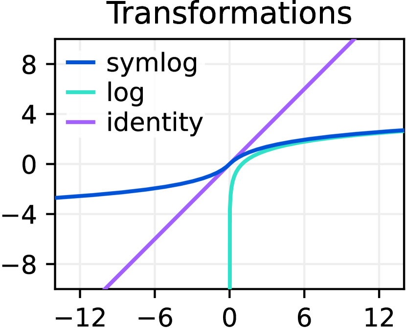
The symlog function compresses the magnitudes of both large positive and negative values. Unlike the logarithm, it is symmetric around the origin while preserving the input sign. This allows the optimization process to quickly move the network predictions to large values when needed. Symlog approximates the identity around the origin so that it does not affect learning of targets that are already small enough. For critic learning, a more involved transformation has previously been proposed ²¹, which we found less effective on average across domains.

DreamerV3 uses symlog predictions in the decoder, the reward predictor, and the critic. It also squashes inputs to the encoder using the symlog function. Despite its simplicity, this approach robustly and quickly learns across a diverse range of environments. With symlog predictions, there is no need for truncating large rewards ¹⁸, introducing non-stationary through reward normalization ¹⁹, or adjusting network weights when new extreme values are detected ²².

World Model Learning

The world model learns compact representations of sensory inputs through autoencoding ²³, ²⁴ and enables planning by predicting future representations and rewards for potential actions. We implement the world model as a Recurrent State-Space Model (RSSM) ¹⁴, as shown in Figure 3. First, an encoder maps sensory inputs $x_{t}$ to stochastic representations $z_{t}$. Then, a sequence model with recurrent state $h_{t}$ predicts the sequence of these representations given past actions $a_{t-1}$. The concatenation of $h_{t}$ and $z_{t}$ forms the model state from which we predict rewards $r_{t}$ and episode continuation flags $c_{t}\in\{0,1\}$ and reconstruct the inputs to ensure informative representations:

$$\begin{aligned} \begin{aligned} \raisebox{8.39578pt}{\hbox to0.0pt{\hss\vbox to0.0pt{\hbox{$\text{RSSM}\hskip 4.30554pt\begin{cases}\hphantom{A}\\ \hphantom{A}\\ \hphantom{A}\end{cases}$}\vss}}}&\text{Sequence model:}\hskip 35.00005pt&&h_{t}&\ =&\ f_{\phi}(h_{t-1},z_{t-1},a_{t-1})\\ &\text{Encoder:}\hskip 35.00005pt&&z_{t}&\ \sim&\ q_{\phi}(z_{t}\;|\;h_{t},x_{t})\\ &\text{Dynamics predictor:}\hskip 35.00005pt&&\hat{z}_{t}&\ \sim&\ p_{\phi}(\hat{z}_{t}\;|\;h_{t})\\ &\text{Reward predictor:}\hskip 35.00005pt&&\hat{r}_{t}&\ \sim&\ p_{\phi}(\hat{r}_{t}\;|\;h_{t},z_{t})\\ &\text{Continue predictor:}\hskip 35.00005pt&&\hat{c}_{t}&\ \sim&\ p_{\phi}(\hat{c}_{t}\;|\;h_{t},z_{t})\\ &\text{Decoder:}\hskip 35.00005pt&&\hat{x}_{t}&\ \sim&\ p_{\phi}(\hat{x}_{t}\;|\;h_{t},z_{t})\end{aligned}\end{aligned}$$ (3)

Figure 5 visualizes long-term video predictions of the world world. The encoder and decoder use convolutional neural networks (CNN) ²⁵ for visual inputs and multi-layer perceptrons (MLPs) for low-dimensional inputs. The dynamics, reward, and continue predictors are also MLPs. The representations are sampled from a vector of softmax distributions and we take straight-through gradients through the sampling step ²⁶, ²⁷. Given a sequence batch of inputs $x_{1:T}$, actions $a_{1:T}$, rewards $r_{1:T}$, and continuation flags $c_{1:T}$, the world model parameters $\phi$ are optimized end-to-end to minimize the prediction loss $\mathcal{L}_{\mathrm{pred}}$, the dynamics loss $\mathcal{L}_{\mathrm{dyn}}$, and the representation loss $\mathcal{L}_{\mathrm{rep}}$ with corresponding loss weights $\beta_{\mathrm{pred}}=1$, $\beta_{\mathrm{dyn}}=0.5$, $\beta_{\mathrm{rep}}=0.1$:

$$\begin{aligned} \mathcal{L}(\phi)\doteq\operatorname{E}_{q_{\phi}}\Big{[}\textstyle\sum_{t=1}^{T}(\beta_{\mathrm{pred}}\mathcal{L}_{\mathrm{pred}}(\phi)+\beta_{\mathrm{dyn}}\mathcal{L}_{\mathrm{dyn}}(\phi)+\beta_{\mathrm{rep}}\mathcal{L}_{\mathrm{rep}}(\phi))\Big{]}.\end{aligned}$$ (4)

Figure 5: Multi-step video predictions in DMLab (top) and Control Suite (bottom). From 5 frames of context input, the model predicts 45 steps into the future given the action sequence and without access to intermediate images. The world model learns an understanding of the underlying 3D structure of the two environments. Refer to Appendix H for additional video predictions.

The prediction loss trains the decoder and reward predictor via the symlog loss and the continue predictor via binary classification loss. The dynamics loss trains the sequence model to predict the next representation by minimizing the KL divergence between the predictor $p_{\phi}(z_{t}\;|\;h_{t})$ and the next stochastic representation $q_{\phi}(z_{t}\;|\;h_{t},x_{t})$. The representation loss trains the representations to become more predictable if the dynamics cannot predict their distribution, allowing us to use a factorized dynamics predictor for fast sampling when training the actor critic. The two losses differ in the stop-gradient operator $\operatorname{sg}(\cdot)$ and their loss scale. To avoid a degenerate solution where the dynamics are trivial to predict but contain not enough information about the inputs, we employ free bits²⁸ by clipping the dynamics and representation losses below the value of 1 nat $\approx$ 1.44 bits. This disables them while they are already minimized well to focus the world model on its prediction loss:

$$\begin{aligned} \mathcal{L_{\mathrm{pred}}}(\phi)&\doteq-\ln p_{\phi}(x_{t}\;|\;z_{t},h_{t})-\ln p_{\phi}(r_{t}\;|\;z_{t},h_{t})-\ln p_{\phi}(c_{t}\;|\;z_{t},h_{t})\\ \mathcal{L_{\mathrm{dyn}}}(\phi)&\doteq\max\bigl{(}1,\operatorname{KL}\!\big{[}\operatorname{sg}(q_{\phi}(z_{t}\;|\;h_{t},x_{t}))\;\big{\|}\;\hskip 13.77771ptp_{\phi}(z_{t}\;|\;h_{t})\hphantom{)}\big{]}\bigr{)}\\ \mathcal{L_{\mathrm{rep}}}(\phi)&\doteq\max\bigl{(}1,\operatorname{KL}\!\big{[}\hskip 13.77771ptq_{\phi}(z_{t}\;|\;h_{t},x_{t})\hphantom{)}\;\big{\|}\;\operatorname{sg}(p_{\phi}(z_{t}\;|\;h_{t}))\big{]}\bigr{)}\end{aligned}$$ (5)

Previous world models require scaling the representation loss differently based on the visual complexity of the environment. Complex 3D environments contain details unnecessary for control and thus prompt a stronger regularizer to simplify the representations and make them more predictable. In 2D games, the background is often static and individual pixels may matter for the task, requiring a weak regularizer to perceive fine details. We find that combining free bits with a small scale for the representation loss resolve this dilemma, allowing for fixed hyperparameters across domains. Moreover, symlog predictions for the decoder unify the gradient scale of the prediction loss across environments, further stabilizing the trade-off with the representation loss.

We occasionally observed spikes the in KL losses in earlier experiments, consistent with reports for deep variational autoencoders ²⁹, ³⁰. To prevent this, we parameterize the categorical distributions of the encoder and dynamics predictor as mixtures of 1% uniform and 99% neural network output, making it impossible for them to become near deterministic and thus ensuring well-scaled KL losses. Further model details and hyperparameters are summarized in Appendix W.

Actor Critic Learning

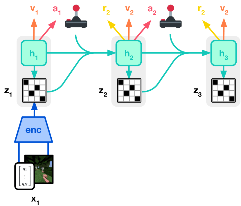
The actor and critic neural networks learn behaviors purely from abstract sequences predicted by the world model ¹², ¹³. During environment interaction, we select actions by sampling from the actor network without lookahead planning. The actor and critic operate on model states $s_{t}\doteq\{h_{t},z_{t}\}$ and thus benefit from the Markovian representations learned by the world model. The actor aims to maximize the expected return $R_{t}\doteq\textstyle\sum_{\tau=0}^{\infty}\gamma^{\tau}r_{t+\tau}$ with a discount factor $\gamma=0.997$ for each model state. To consider rewards beyond the prediction horizon $T=16$, the critic learns to predict the return of each state under the current actor behavior:

$$\begin{aligned} &\text{Actor:}\quad&&a_{t}\sim\pi_{\theta}(a_{t}\;|\;s_{t})\\ &\text{Critic:}\quad&&v_{\psi}(s_{t})\approx\operatorname{E}_{p_{\phi},\pi_{\theta}}\big{[}R_{t}\big{]}\end{aligned}$$ (6)

Starting from representations of replayed inputs, the dynamics predictor and actor produce a sequence of imagined model states $s_{1:T}$, actions $a_{1:T}$, rewards $r_{1:T}$, and continuation flags $c_{1:T}$. To estimate returns that consider rewards beyond the prediction horizon, we compute bootstrapped $\lambda$-returns that integrate the predicted rewards and values ³¹, ³²:

$$\begin{aligned} R^{\lambda}_{t}\doteq r_{t}+\gamma c_{t}\Big{(}(1-\lambda)v_{\psi}(s_{t+1})+\lambda R^{\lambda}_{t+1}\Big{)}\qquad R^{\lambda}_{T}\doteq v_{\psi}(s_{T})\end{aligned}$$ (7)

Critic Learning

A simple choice for the critic loss function would be to regress the $\lambda$-returns via squared error or symlog predictions. However, the critic predicts the expected value of a potentially widespread return distribution, which can slow down learning. We choose a discrete regression approach for learning the critic based on twohot encoded targets ³³, ³⁴, ³⁵, ³⁶ that let the critic maintain and refine a distribution over potential returns. For this, we transform returns using the symlog function and discretize the resulting range into a sequence $B$ of $K=255$ equally spaced buckets $b_{i}$. The critic network outputs a softmax distribution $p_{\psi}(b_{i}\;|\;s_{t})$ over the buckets and its output is formed as the expected bucket value under this distribution. Importantly, the critic can predict any continuous value in the interval because its expected bucket value can fall between the buckets:

$$\begin{aligned} v_{\psi}(s_{t})\doteq\operatorname{symexp}(\operatorname{E}_{p_{\psi}(b_{i}\;|\;s_{t})}\big{[}b_{i}\big{]})=\operatorname{symexp}(p_{\psi}(\cdot\;|\;s_{t})^{T}B)\qquad B\doteq\begin{bmatrix}-20&...&+20\end{bmatrix}\end{aligned}$$ (8)

To train the critic, we symlog transform the targets $R^{\lambda}_{t}$ and then twohot encode them into a soft label for the softmax distribution produced by the critic. Twohot encoding is a generalization of onehot encoding to continuous values. It produces a vector of length $|B|$ where all elements are $0$ except for the two entries closest to the encoded continuous number, at positions $k$ and $k+1$. These two entries sum up to $1$, with more weight given to the entry that is closer to the encoded number:

$$\begin{aligned} \operatorname{twohot}(x)_{i}\doteq\begin{cases}|b_{k+1}-x|\,/\,|b_{k+1}-b_{k}|&\text{ if }i=k\\ |b_{k\hphantom{+1}}-x|\,/\,|b_{k+1}-b_{k}|&\text{ if }i=k+1\\ 0&\text{ else}\\ \end{cases}\qquad k\doteq\sum_{j=1}^{B}\operatorname{\delta}(b_{j}<x)\end{aligned}$$ (9)

Given twohot encoded targets $y_{t}=\operatorname{sg}(\operatorname{twohot}(\operatorname{symlog}(R^{\lambda}_{t})))$, where $\operatorname{sg}(\cdot)$ stops the gradient, the critic minimizes the categorical cross entropy loss for classification with soft targets:

$$\begin{aligned} \mathcal{L}_{\mathrm{critic}}(\psi)\doteq\sum_{t=1}^{T}\operatorname{E}_{b_{i}\sim y_{t}}\big{[}-\lnp_{\psi}(b_{i}\;\big{|}\;s_{t})\big{]}=-\sum_{t=1}^{T}y_{t}^{T}\ln p_{\psi}(\cdot\;|\;s_{t})\end{aligned}$$ (10)

We found discrete regression for the critic to accelerate learning especially in environments with sparse rewards, likely because of their bimodal reward and return distributions. We use the same discrete regression approach for the reward predictor of the world model.

Because the critic regresses targets that depend on its own predictions, we stabilize learning by regularizing the critic towards predicting the outputs of an exponentially moving average of its own parameters. This is similar to target networks used previously in reinforcement learning ¹⁸ but allows us to compute returns using the current critic network. We further noticed that the randomly initialized reward predictor and critic networks at the start of training can result in large predicted rewards that can delay the onset of learning. We initialize the output weights of the reward predictor and critic to zeros, which effectively alleviates the problem and accelerates early learning.

Actor Learning

The actor network learns to choose actions that maximize returns while ensuring sufficient exploration through an entropy regularizer ³⁷. However, the scale of this regularizer heavily depends on the scale and frequency of rewards in the environment, which has been a challenge for previous algorithms ³⁸. Ideally, we would like the policy to explore quickly in the absence of nearby returns without sacrificing final performance under dense returns.

To stabilize the scale of returns, we normalize them using moving statistics. For tasks with dense rewards, one can simply divide returns by their standard deviation, similar to previous work ¹⁹. However, when rewards are sparse, the return standard deviation is generally small and this approach would amplify the noise contained in near-zero returns, resulting in an overly deterministic policy that fails to explore. Therefore, we propose propose to scale down large returns without scaling up small returns. We implement this idea by dividing returns by their scale $S$, for which we discuss multiple choices below, but only if they exceed a minimum threshold of $1$. This simple change is the key to allowing a single entropy scale $\eta=3\cdot 10^{-4}$ across dense and sparse rewards:

$$\begin{aligned} \mathcal{L}(\theta)\doteq\textstyle\sum_{t=1}^{T}\operatorname{E}_{\pi_{\theta},p_{\phi}}\big{[}\operatorname{sg}(R^{\lambda}_{t})/\max(1,S)\big{]}-\,\eta\operatorname{H}\big{[}\pi_{\theta}(a_{t}\;\big{|}\;s_{t})\big{]}\end{aligned}$$ (11)

We follow DreamerV2 ²⁷ in estimating the gradient of the first term by stochastic backpropagation for continuous actions and by reinforce ³⁹ for discrete actions. The gradient of the second term is computed in closed form.

In deterministic environments, we find that normalizing returns by their exponentially decaying standard deviation suffices. However, for heavily randomized environments, the return distribution can be highly non-Gaussian and contain outliers of large returns caused by a small number of particularly easy episodes, leading to an overly deterministic policy that struggles to sufficiently explore. To normalize returns while being robust to such outliers, we scale returns by an exponentially decaying average of the range from their 5^th to their 95^th batch percentile:

$$\begin{aligned} S=\operatorname{Per}(R^{\lambda}_{t},95)-\operatorname{Per}(R^{\lambda}_{t},5)\end{aligned}$$ (12)

Because a constant return offset does not affect the objective, this is equivalent to an affine transformation that maps these percentiles to $0$ and $1$, respectively. Compared to advantage normalization ¹⁹, scaling returns down accelerates exploration under sparse rewards without sacrificing final performance under dense rewards, while using a fixed entropy scale.

(a) Training Ratio

(b) Model Size

Figure 6: Scaling properties of DreamerV3. The graphs show task performance over environment steps for different training ratios and model sizes reaching from 8M to 200M parameters. The training ratio is the ratio of replayed steps to environment steps. The model sizes are detailed in Appendix B. Higher training ratios result in substantially improved data-efficiency. Notably, larger models achieve not only higher final performance but also higher data-efficiency.

Results

We perform an extensive empirical study to evaluate the generality and scalability of DreamerV3 across diverse domains—with over 150 tasks—under fixed hyperparameters. We designed the experiments to compare DreamerV3 to the best methods in the literature, which are often specifically designed to the benchmark at hand. Moreover, we apply DreamerV3 to the challenging video game Minecraft. Appendix A gives an overview of the domains. For DreamerV3, we directly report the performance of the stochastic training policy and avoid separate evaluation runs using the deterministic policy, simplifying the setup. All DreamerV3 agents are trained on one Nvidia V100 GPU each, making the algorithm widely usable across research labs. The source code and numerical results are available on the project website: https://danijar.com/dreamerv3

Benchmarks

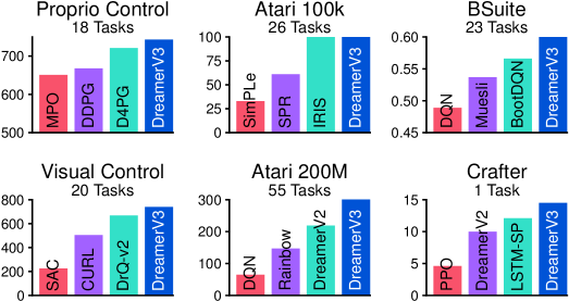
To evaluate the generality of DreamerV3, we perform an extensive empirical evaluation across 7 domains that include continuous and discrete actions, visual and low-dimensional inputs, dense and sparse rewards, different reward scales, 2D and 3D worlds, and procedural generation. Figure 1 summarizes the results, with training curves and score tables included in the appendix. DreamerV3 achieves strong performance on all domains and outperforms all previous algorithms on 4 of them, while also using fixed hyperparameters across all benchmarks.

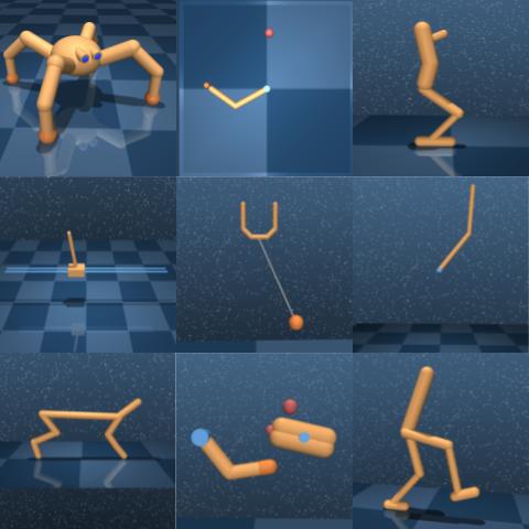
• Proprio Control Suite  This benchmark contains 18 continuous control tasks with low-dimensional inputs and a budget of 500K environment steps ⁴⁰. The tasks range from classical control over locomotion to robot manipulation tasks. DreamerV3 sets a new state-of-the-art on this benchmark, outperforming D4PG ⁴¹, DMPO ⁴², and MPO ⁴³.

• Visual Control Suite  This benchmark consists of 20 continuous control tasks where the agent receives only high-dimensional images as inputs and a budget of 1M environment steps ⁴⁰, ²⁷. DreamerV3 establishes a new state-of-the-art on this benchmark, outperforming DrQ-v2 ⁴⁴ and CURL ⁴⁵ which additionally require data augmentations.

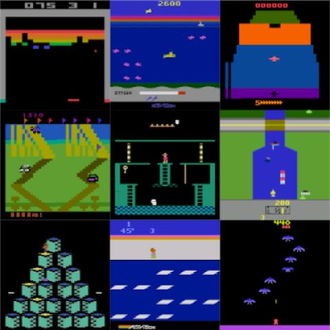
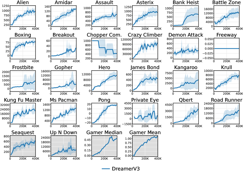
• Atari 100k  This benchmark includes 26 Atari games and a budget of only 400K environment steps, amounting to 100K steps after action repeat or 2 hours of real time ⁴⁶. EfficientZero ⁴⁷ holds the state-of-the-art on this benchmark by combining online tree search, prioritized replay, hyperparameter scheduling, and allowing early resets of the games; see Appendix T for an overview. Without this complexity, DreamerV3 outperforms the remaining previous methods such as the transformer-based IRIS ⁴⁸, the model-free SPR ⁴⁹, and SimPLe ⁴⁶.

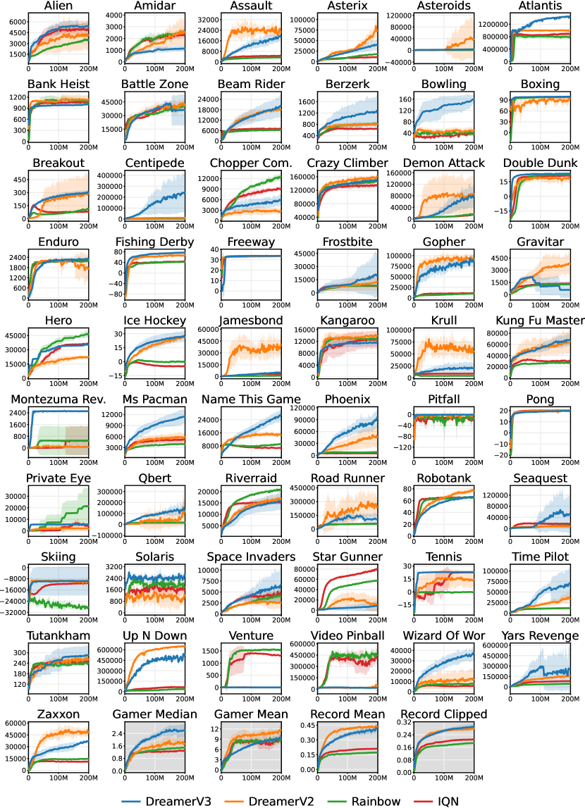
• Atari 200M  This popular benchmark includes 55 Atari video games with simple graphics and a budget of 200M environment steps ⁵⁰. We use the sticky action setting ⁵¹. DreamerV3 outperforms DreamerV2 with a median score of 302% compared to 219%, as well as the top model-free algorithms Rainbow ⁵² and IQN ⁵³ that were specifically designed for the Atari benchmark.

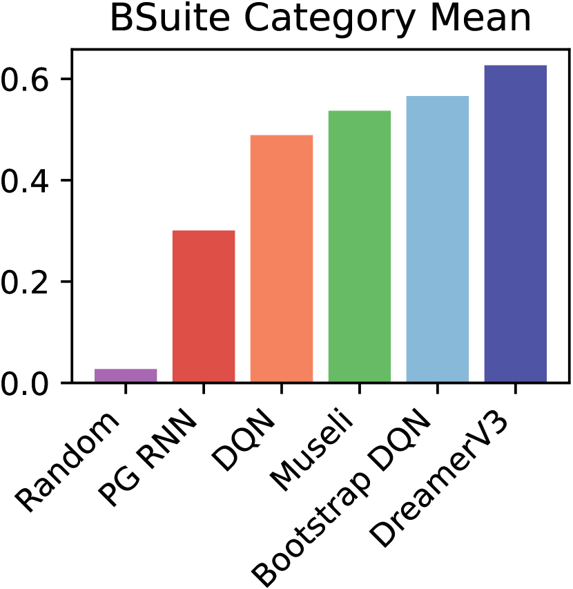
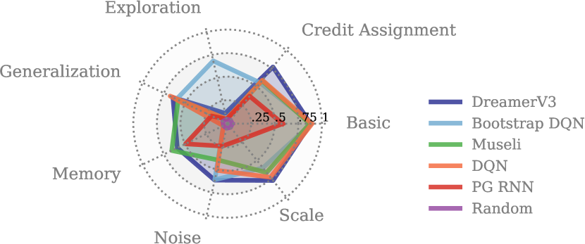
• BSuite  This benchmark includes 23 environments with a total of 468 configurations that are designed to test credit assignment, robustness to reward scale and stochasticity, memory, generalization, and exploration ⁵⁴. DreamerV3 establishes a new state-of-the-art on this benchmark, outperforming Bootstrap DQN ⁵⁵ as well as Muesli ⁵⁶ with comparable amount of training. DreamerV3 improves over previous algorithms the most in the credit assignment category.

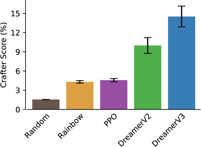
• Crafter  This procedurally generated survival environment with top-down graphics and discrete actions is designed to evaluate a broad range of agent abilities, including wide and deep exploration, long-term reasoning and credit assignment, and generalization ⁵⁷. DreamerV3 sets a new state-of-the-art on this benchmark, outperforming PPO with the LSTM-SPCNN architecture ⁵⁸, the object-centric OC-SA ⁵⁸, DreamerV2 ²⁷, and Rainbow ⁵².

• 

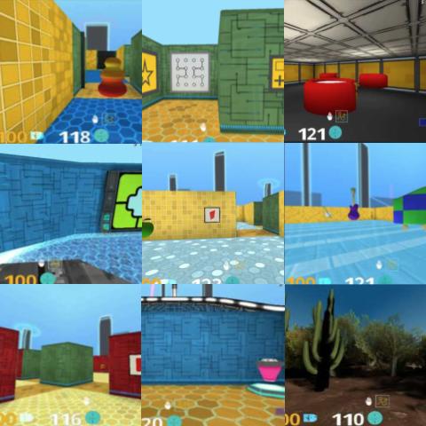
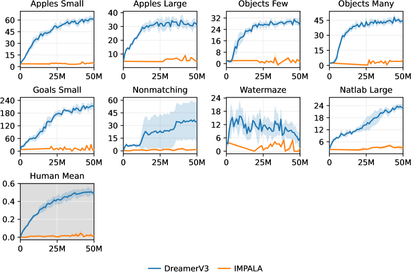
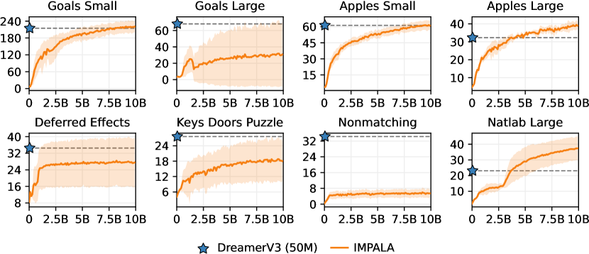
  DMLab This domain contains 3D environments that require spatial and temporal reasoning ⁵⁹. On 8 challenging tasks, DreamerV3 matches and exceeds the final performance on the scalable IMPALA agent ⁶⁰ in only 50M compared to 10B environment steps, amounting to a data-efficiency gain of over 13000%. We note that IMPALA was not designed for data-efficiency but serves as a valuable baseline for the performance achievable by scalable RL algorithms without data constraints.

Scaling properties

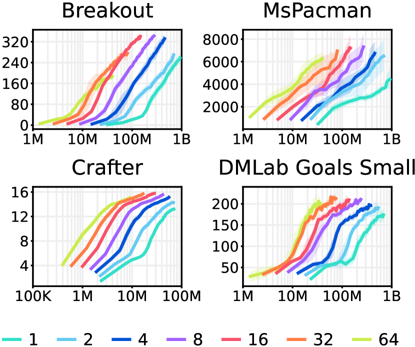
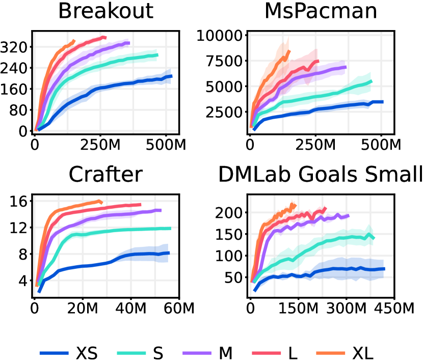
Solving challenging tasks out of the box not only requires an algorithm that succeeds without adjusting hyperparameters, but also the ability to leverage large models to solve hard tasks. To investigate the scaling properties of DreamerV3, we train 5 model sizes ranging from 8M to 200M parameters. As shown in Figure 6, we discover favorable scaling properties where increasing the model size directly translates to both higher final performance and data-efficiency. Increasing the number of gradient steps further reduces the number of interactions needed to learn successful behaviors. These insights serve as practical guidance for applying DreamerV3 to new tasks and demonstrate the robustness and scalability of the algorithm.

Minecraft

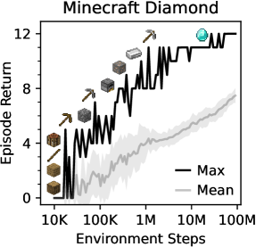
Collecting diamonds in the open-world game Minecraft has been a long-standing challenge in artificial intelligence. Every episode in this game is set in a different procedurally generated 3D world, where the player needs to discover a sequence of 12 milestones with sparse rewards by foraging for resources and using them to craft tools. The environment is detailed in Appendix F. We following prior work ¹⁷ and increase the speed at which blocks break because a stochastic policy is unlikely to sample the same action often enough in a row to break blocks without regressing its progress by sampling a different action.

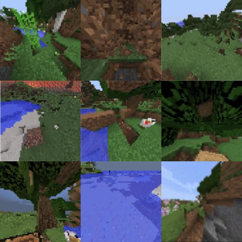
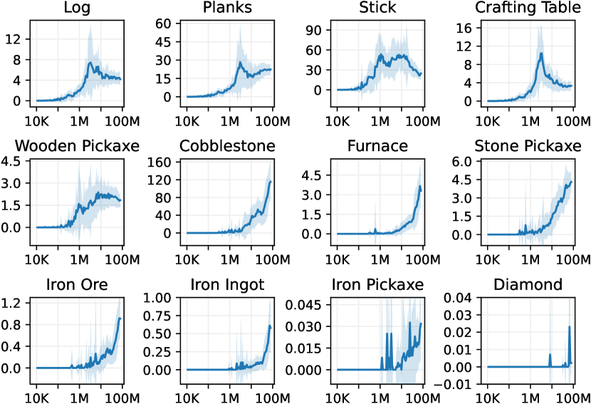
Because of the training time in this complex domain, tuning algorithms specifically for Minecraft would be difficult. Instead, we apply DreamerV3 out of the box with its default hyperparameters. As shown in Figure 1, DreamerV3 is the first algorithm to collect diamonds in Minecraft from scratch without using human data that was required by VPT ¹⁶. Across 40 seeds trained for 100M environment steps, DreamerV3 collects diamonds in 50 episode. It collects the first diamond after 29M steps and the frequency increases as training progresses. A total of 24 of the 40 seeds collect at least one diamond and the most successful agent collects diamonds in 6 episodes. The success rates for all 12 milestones are shown in Figure G.1.

Previous Work

Developing general-purpose algorithms has long been a goal of reinforcement learning research. PPO ¹⁹ is one of the most widely used algorithms and requires relatively little tuning but uses large amounts of experience due to its on-policy nature. SAC ³⁸ is a popular choice for continuous control and leverages experience replay for higher data-efficiency, but in practice requires tuning, especially for its entropy scale, and struggles with high-dimensional inputs ⁶¹. MuZero ³⁴ plans using a value prediction model and has achieved high performance at the cost of complex algorithmic components, such as MCTS with UCB exploration and prioritized replay. Gato ⁶² fits one large model to expert demonstrations of multiple tasks, but is only applicable to tasks where expert data is available. In comparison, we show that DreamerV3 masters a diverse range of environments trained with fixed hyperparameters and from scratch.

Minecraft has been a focus of recent reinforcement learning research. With MALMO ⁶³, Microsoft released a free version of the popular game for research purposes. MineRL ¹⁵ offers several competition environments, which we rely on as the basis for our experiments. MineDojo ⁶⁴ provides a large catalog of tasks with sparse rewards and language descriptions. The yearly MineRL competition supports agents in exploring and learning meaningful skills through a diverse human dataset ¹⁵. VPT ¹⁶ trained an agent to play Minecraft through behavioral cloning of expert data collected by contractors and finetuning using reinforcement learning, resulting in a 2.5% success rate of diamonds using 720 V100 GPUs for 9 days. In comparison, DreamerV3 learns to collect diamonds in 17 GPU days from sparse rewards and without human data.

Conclusion

This paper presents DreamerV3, a general and scalable reinforcement learning algorithm that masters a wide range of domains with fixed hyperparameters. To achieve this, we systematically address varying signal magnitudes and instabilities in all of its components. DreamerV3 succeeds across 7 benchmarks and establishes a new state-of-the-art on continuous control from states and images, on BSuite, and on Crafter. Moreover, DreamerV3 learns successfully in 3D environments that require spatial and temporal reasoning, outperforming IMPALA in DMLab tasks using 130 times fewer interactions and being the first algorithm to obtain diamonds in Minecraft end-to-end from sparse rewards. Finally, we demonstrate that the final performance and data-efficiency of DreamerV3 improve monotonically as a function of model size.

Limitations of our work include that DreamerV3 only learns to sometimes collect diamonds in Minecraft within 100M environment steps, rather than during every episode. Despite some procedurally generated worlds being more difficult than others, human experts can typically collect diamonds in all scenarios. Moreover, we increase the speed at which blocks break to allow learning Minecraft with a stochastic policy, which could be addressed through inductive biases in prior work. To show how far the scaling properties of DreamerV3 extrapolate, future implementations at larger scale are necessary. In this work, we trained separate agents for all tasks. World models carry the potential for substantial transfer between tasks. Therefore, we see training larger models to solve multiple tasks across overlapping domains as a promising direction for future investigations.

Acknowledgements

We thank Oleh Rybkin, Mohammad Norouzi, Abbas Abdolmaleki, John Schulman, and Adam Kosiorek for insightful discussions. We thank Bobak Shahriari for training curves of baselines for proprioceptive control, Denis Yarats for training curves for visual control, Surya Bhupatiraju for Muesli results on BSuite, and Hubert Soyer for providing training curves of the original IMPALA experiments. We thank Daniel Furrer, Andrew Chen, and Dakshesh Garambha for help with using Google Cloud infrastructure for running the Minecraft experiments.

Appendices

psection[2.3em]2.3em [sections] [sections]p1

Appendix A Benchmark Overview

colspec = | L6em | C3.5em C3.5em C3.5em C3.5em C3.5em C3.5em C3.5em |, row1 = font=,

Benchmark
Tasks Env Steps Action Repeat Env Instances Train Ratio GPU Days Model Size
DMC Proprio 18 500K 2 4 512 0<1 S
DMC Vision 20 1M 2 4 512 0<1 S
Crafter 1 1M 1 1 512 02 XL
BSuite 23 — 1 1 1024 0<1 XL
Atari 100K 26 400K 4 1 1024 0<1 S
Atari 200M 55 200M 4 8 64 16 XL
DMLab 8 50M 4 8 64 04 XL
Minecraft 1 100M 1 16 16 17 XL

Table A.1: Benchmark overview. The train ratio is the number of replayed steps per policy steps rather than environment steps, and thus unaware of the action repeat. BSuite sets the number of episodes rather than env steps, both of which vary across tasks. BSuite requires multiple configurations per environment and one seed per configuration, resulting in 468 runs. For DMC, the proprioceptive benchmark excludes the quadruped tasks that are present in the visual benchmark because of baseline availability in prior work. All agents were trained on 1 Nvidia V100 GPU each.

Appendix B Model Sizes

colspec = | L10em | C4.5em C4.5em C4.5em C4.5em C4.5em |, row1 = font=,

Dimension XS S M L XL
GRU recurrent units 256 512 1024 2048 4096
CNN multiplier 24 32 48 64 96
Dense hidden units 256 512 640 768 1024
MLP layers 1 2 3 4 5
Parameters 8M 18M 37M 77M 200M

Table B.1: Model sizes. The encoder consists of stride 2 convolutions of doubling depth until resolution $4\times 4$ followed by flattening. The decoder starts with a dense layer, followed by reshaping to $4\times 4\times C$ and then inverts the encoder architecture. The dynamics are implemented as RSSM with vectors of categorical representations, consisting of a GRU and dense layers.

Appendix C Summary of Differences

DreamerV3 builds upon the DreamerV2 algorithm ²⁷. This section describes the main changes that we applied in order to master a wide range of domains with fixed hyperparameters and enable robust learning on unseen domains.

• Symlog predictions  We symlog encode inputs to the world model and use symlog predictions with squared error for reconstructing inputs. The reward predictor and critic use twohot symlog predictions, a simple form of distributional reinforcement learning ³³.

• World model regularizer  We experimented with different approaches for removing the need to tune the KL regularizer, including targeting a fixed KL value. A simple yet effective solution turned out to combine KL balancing that was introduced in DreamerV2 ²⁷ with free bits ²⁸ that were used in the original Dreamer algorithm ⁶⁵. GECO ⁶⁶ was not useful in our case because what constitutes “good” reconstruction error varies widely across domains.

• Policy regularizer  Using a fixed entropy regularizer for the actor was challenging when targeting both dense and sparse rewards. Scaling large return ranges down to the $[0,1]$ interval, without amplifying near-zero returns, overcame this challenge. Using percentiles to ignore outliers in the return range further helped, especially for stochastic environments. We did not experience improvements from regularizing the policy towards its own EMA ⁶⁷ or the CMPO regularizer ⁵⁶.

• Unimix categoricals  We parameterize the categorical distributions for the world model representations and dynamics, as well as for the actor network, as mixtures of 1% uniform and 99% neural network output ⁶⁸, ⁶⁹ to ensure a minimal amount of probability mass on every class and thus keep log probabilities and KL divergences well behaved.

• Architecture  We use a similar network architecture but employ layer normalization ⁷⁰ and SiLU ⁷¹ as the activation function. For better framework support, we use same-padded convolutions with stride 2 and kernel size 3 instead of valid-padded convolutions with larger kernels. The robustness of DreamerV3 allowed us to use large networks that contributed to its performance.

• Critic EMA regularizer  We compute $\lambda$-returns using the fast critic network and regularize the critic outputs towards those of its own weight EMA instead of computing returns using the slow critic. However, both approaches perform similarly in practice.

• Replay buffer  DreamerV2 used a replay buffer that only replays time steps from completed episodes. To shorten the feedback loop, DreamerV3 uniformly samples from all inserted subsequences of size batch length regardless of episode boundaries.

• Hyperparameters  The hyperparameters of DreamerV3 were tuned to perform well across both the visual control suite and Atari 200M at the same time. We verified their generality by training on new domains without further adjustment, including Crafter, BSuite, and Minecraft.

Target Regularizers

We also experimented with constrained optimization for the world model and policy objectives, where we set a target value that the regularizer should take on, on average across states. We found combining this approach with limits on the allowed regularizer scales to perform well for the world model, at the cost of additional complexity. For the actor, choosing a target randomness of $40\%$—where $0\%$ corresponds to the most deterministic and $100\%$ to the most random policy—learns robustly across domains but prevents the policy from converging to top scores in tasks that require speed or precision and slows down exploration under sparse rewards. The solutions in DreamerV3 do not have these issues intrinsic to constrained optimization formulations.

Appendix D Ablation Curves

Figure D.1: World Model ablations. KL balancing ²⁷ subsantially accelerates learning. Free bits ²⁸, ⁶⁵ avoids overfitting in simple environments. Symlog encoding and predictions for proprioceptive observations speeds up learning. Adjusting the KL scale over the course of training within a reasonable range to target a fixed KL value is a performant but more complicated alternative to free bits.

Figure D.2: Critic ablations. The symlog predictions for rewards and values in DreamerV3 outperform non-stationary reward normalization. Discrete regression also contributes significantly ³⁴. Symlog transformation slightly outperforms the more complex asymmetric square root transformation of R2D2 ²¹. Using the slow critic for computing targets offers no benefit over using the fast critic and regularizing it towards its own EMA.

Figure D.3: Actor ablations. The strength of the actor entropy regularizer is important especially under sparse rewards, where the right amount of stochasticity is needed for exploration. The denominator maximum that prevents small returns (often noise) from being amplified is critical. The percentile return normalization of DreamerV3 outperforms normalization based on return stddev or advantage stddev on the sparse reward tasks ⁷².

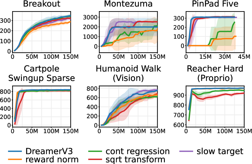
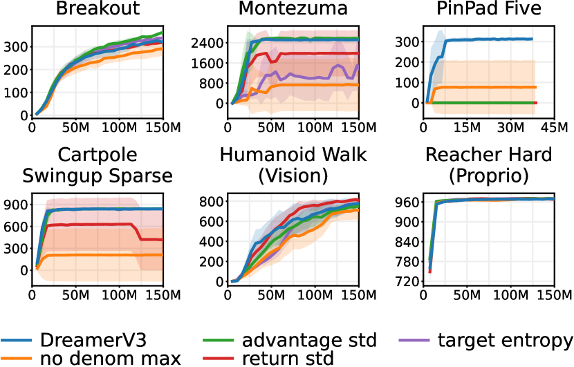
Appendix E Ablation Explanation

World Model Ablations

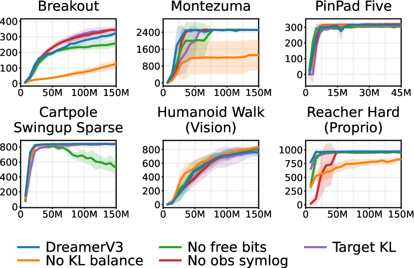
NoFreeBits

Use KL balancing but no free bits, equivalent to setting the constants in Equation 4 from 1 to 0. This objective was used in DreamerV2 ²⁷.

NoKLBalance

Use free bits but no KL balancing by setting $\beta_{\mathrm{dyn}}=\beta_{\mathrm{dyn}}=0.5$, which recovers the $\beta$-VAE objective ⁷³. We found this value to perform well compared to nearby values. This objective was used in the first Dreamer agent ⁶⁵.

NoObsSymlog

This ablation removes the symlog encoding of inputs to the world model and also changes the symlog MSE loss in the decoder to a simple MSE loss. Because symlog encoding is only used for vector observations, this ablation is equivalent to DreamerV3 on purely image-based environments.

TargetKL

Target a KL value of 3.5 nats on average over the replay buffer by increasing or decreasing the KL scale (both $\beta_{\mathrm{pred}}$ and $\beta_{\mathrm{rep}}$) by 10% when the batch average of the KL value exceeds or falls below the tolerance of 10% around the target value, similar to the KL-penalty variant of PPO ¹⁹. The KL scale is limited to the range $[10^{-3},1.0]$ for numerical stability.

Critic Ablations

RewardNorm

Instead of normalizing rewards, normalize rewards by dividing them by a running standard deviation and clipping them beyond a magnitude of 10.

ContRegression

Using MSE symlog predictions for the reward and value heads.

SqrtTransform

Using two-hot discrete regression with the asymmetric square root transformation introduced by R2D2 ²¹ and used in MuZero ³⁴.

SlowTarget

Instead of using the fast critic for computing returns and training it towards the slow critic, use the slow critic for computing returns ¹⁸.

Actor Ablations

NoDenomMax

Normalize returns directly based on the range between percentiles 5 to 95 with a small epsilon in the denominator, instead of by the maximum of 1 and the percentile range. This way, not only large returns are scaled down but also small returns are scaled up.

AdvantageStd

Advantage normalization as commonly used, for example in PPO ¹⁹ and Muesli ⁵⁶. However, scaling advantages without also scaling the entropy regularizer changes the trade-off between return and entropy in a way that depends on the scale of advantages, which in turn depends on how well the critic currently predicts the returns.

ReturnStd

Instead of normalizing returns by the range between percentiles 5 to 95, normalize them by their standard deviation. When rewards are large but sparse, the standard deviation is small, scaling up the few large returns even further.

TargetEntropy

Target a policy randomness of 40% on average across imagined states by increasing or decreasing the entropy scale $\eta$ by 10% when the batch average of the randomness falls below or exceeds the tolerance of 10% around the target value. The entropy scale is limited to the range $[10^{-3},3\cdot 10^{-2}]$. Policy randomness is the policy entropy mapped to range from 0% (most deterministic allowed by action distribution parameterization) to 100% (most uniform). Multiplicatively, instead of additively, adjusting the regularizer strength allows the scale to quickly move across orders of magnitude, outperforming the target entropy approach of SAC ³⁸ in practice. Moreover, targeting a randomness value rather than an entropy value allows sharing the hyperparameter across domains with discrete and continuous actions.

Appendix F Minecraft Environment

Minecraft

With 100M monthly active users, Minecraft is one of the most popular video games worldwide. Minecraft features a procedurally generated 3D world of different biomes, including plains, forests, jungles, mountains, deserts, taiga, snowy tundra, ice spikes, swamps, savannahs, badlands, beaches, stone shores, rivers, and oceans. The world consists of 1 meter sized blocks that the player and break and place. There are about 30 different creatures that the player can interact and fight with. From gathered resources, the player can use 379 recipes to craft new items and progress through the technology tree, all while ensuring safety and food supply to survive. There are many conceivable tasks in Minecraft and as a first step, the research community has focused on the salient task of obtaining a diamonds, a rare item found deep underground and requires progressing through the technology tree.

Environment

We built the Minecraft Diamond environment on top of MineRL to define a flat categorical action space and fix issues we discovered with the original environments via human play testing. For example, when breaking diamond ore, the item sometimes jumps into the inventory and sometimes needs to be collected from the ground. The original environment terminates episodes when breaking diamond ore so that many successful episodes end before collecting the item and thus without the reward. We remove this early termination condition and end episodes when the player dies or after 36000 steps, corresponding to 30 minutes at the control frequency of 20Hz. Another issue is that the jump action has to be held for longer than one control step to trigger a jump, which we solve by keeping the key pressed in the background for 200ms. We built the environment on top of MineRL v0.4.4 ¹⁵, which offers abstract crafting actions. The Minecraft version is 1.11.2.

Rewards

We follow the same sparse reward structure of the MineRL competition environment that rewards 12 milestones leading up to the diamond, namely collecting the items log, plank, stick, crafting table, wooden pickaxe, cobblestone, stone pickaxe, iron ore, furnace, iron ingot, iron pickaxe, and diamond. The reward for each item is only given once per episode, and the agent has to learn autonomously that it needs to collect some of the items multiple times to achieve the next milestone. To make the return curves easy to interpret, we give a reward of $+1$ for each milestone instead of scaling rewards based on how valuable each item is. Additionally, we give a small reward of $-0.01$ for each lost heart and $+0.01$ for each restored heart, but we did not investigate whether this was helpful.

Inputs

The sensory inputs include the $64\times 64\times 3$ RGB first-person camera image, the inventory counts as a vector with one entry for each of the game’s over 400 items, the vector of maximum inventory counts since episode begin to tell the agent which milestones it has already achieved, a one-hot vector indicating the equipped item, and scalar inputs for the health, hunger, and breath levels.

Actions

The MineRL environment provides a dictionary action space and delegates choosing a simple action space to the user. We use a flat categorical action space with 25 actions for walking in four directions, turning the camera in four directions, attacking, jumping, placing items, crafting items near a placed crafting table, smelting items near a placed furnace, and equipping crafted tools. Looking up and down is restricted to the range $-60$ to $+60$ degrees. The action space is specific to the diamond task and does not allow the agent to craft all of the 379 recipes. For multi-task learning, a larger factorized action space as available in MineDojo ⁶⁴ would likely be beneficial.

Break Speed Multiplier

We follow Kanitscheider et al. ¹⁷ in allowing the agent to break blocks in fewer time steps. Breaking blocks in Minecraft requires holding the same key pressed for sometimes hundreds of time steps. Briefly switching to a different key will reset this progress. Without an inductive bias, stochastic policies will almost never sample the same action this often during exploration under this parameterization. To circumvent this issue, we set the break speed multiplier option of MineRL to 100. In the future, inductive biases such as learning action repeat as part of the agent ⁷⁴ could overcome this caveat.

Appendix G Minecraft Item Rates

Across 40 seeds trained for 100M steps, DreamerV3 obtained the maximum episode score—that includes collecting at least one diamond—50 times. It achieves this score the first time at 29.3M steps and as expected the frequency increases over time. Diamonds can also rarely be found by breaking village chests, but those episodes do not achieve the maximum score and thus are not included in this statistic. A total of 24 out of 40 seeds achieve the maximum episode score at least once, and the most successful seed achieved the maximum score 6 times. Across all seeds, the median number of environment steps until collecting the first diamond is 74M, corresponding to 42 days of play time at 20 Hz.

Figure G.1: Minecraft episode counts of rewarded items. Despite receiving only one sparse reward per item within the same episode, the agent learns that some items are requires multiple times to unlock later milestones. Later during training, the agent becomes more efficient and creates fewer additional items. Across all 40 seeds, DreamerV3 discovers a total of 116 unique items in Minecraft.

Appendix H Minecraft Video Predictions

Figure H.1: Multi-step predictions on Minecraft. The model receives the first 5 frames as context input and the predicts 45 steps into the future given the action sequence and without access to intermediate images.

Appendix I DMLab Curves

Figure I.1: DMLab scores with a budget of 50M frames. Separate agents were trained for each task, corresponding to the IMPALA Experts method in Espeholt et al. ⁶⁰. Data efficiency is not the goal of IMPALA and it might be possible to tune it for improved data efficiency. Longer training curves and asymptotic performance of IMPALA are included in Appendix K.

Appendix J DMLab Scores

colspec = | L9em | C4em C4em | C5em C5em | C5em |, row1 = font=,

Task Random Human IMPALA DreamerV3 IMPALA
Environment Steps — — 50M 50M 10B
Goals Small 7.7 267.5 05.7 214.7 209.4
Goals Large 3.1 194.5 03.7 068.1 083.1
Apples Small 3.6 074.5 03.7 061.3 057.8
Apples Large 4.7 065.7 05.0 032.3 037.0
Deferred Effects 8.5 085.7 11.4 034.5 015.6
Keys Doors Puzzle 4.1 053.8 05.1 027.6 028.0
Nonmatching 0.3 065.9 01.8 034.3 007.3
Natlab Large 2.2 036.9 02.4 023.1 034.7
Normalized Mean 0.0% 100.0% 1.1% 54.2% 51.3%

Table J.1: DMLab scores. DreamerV3 achieves a human-normalized mean score of $54.2\%$ that exceeds IMPALA at $51.3\%$ while using 200 times fewer environment steps.

Appendix K DMLab Data Efficiency

Figure K.1: IMPALA training curves on DMLab for 10 billion frames compared to DreamerV3 score. DreamerV3 uses 100$\times$ fewer frames, which is almost at the left edge of the plot, as shown by the markers. Note that data efficiency was not the goal of IMPALA. Instead, it serves as a valuable baseline for the performance achievable by top RL algorithms without data constraints.

colspec = | L8em | C8em C8em C8em |, row1 = font=,

Task DreamerV3 IMPALA Steps Ratio
Goals Small 214.7 8.0B 80$\times$
Goals Large 68.1 — $>$200$\times$
Apples Small 61.3 9.7B 97$\times$
Apples Large 32.3 4.1B 41$\times$
Deferred Effects 34.5 — $>$200$\times$
Keys Doors Puzzle 27.6 — $>$200$\times$
Nonmatching 34.3 — $>$200$\times$
Natlab Large 23.1 3.7B 37$\times$

Table K.1: Data-efficiency comparison of DreamerV3 and IMPALA. The columns shows the score of DreamerV3 after 50M frames, how many steps IMPALA takes to reach the same score, and the resulting data-efficiency gain of DreamerV3 over IMPALA. The nonmatching task is excluded because DreamerV3 outperforms the final score of IMPALA here. The average efficiency gain across tasks is over 131.87$\times$

Appendix L BSuite Scores

Figure L.1: BSuite scores averaged over categories and per category. The benchmark aggregates a total of 468 task configurations. The comparably high score of BootDQN is due to its ability to solve the exploration tasks in BSuite.

colspec = | L11em L12.5em | C5.5em | C5.5em |, row1 = font=,

Task Categories Muesli DreamerV3
bandit basic 0.908 0.859
bandit_noise noise 0.721 0.602
bandit_scale scale 0.674 0.680
cartpole basic, credit., generalization 0.906 0.853
cartpole_noise noise, generalization 0.841 0.664
cartpole_scale scale, generalization 0.701 0.779
cartpole_swingup exploration, generalization 0.000 0.000
catch basic, credit assignment 0.955 0.970
catch_noise noise, credit assignment 0.464 0.571
catch_scale scale, credit assignment 0.929 0.977
deep_sea exploration 0.000 0.000
deep_sea_stochastic exploration, noise 0.000 0.341
discounting_chain credit assignment 0.453 0.290
memory_len memory 0.609 0.478
memory_size memory 0.706 0.706
mnist basic, generalization 0.790 0.762
mnist_noise noise, generalization 0.334 0.416
mnist_scale scale, generalization 0.615 0.477
mountain_car basic, generalization 0.797 0.949
mountain_car_noise noise, generalization 0.441 0.590
mountain_car_scale scale, generalization 0.400 0.948
umbrella_distract credit assignment, noise 0.217 0.957
umbrella_length credit assignment, noise 0.173 0.783
Category mean 0.537 0.627

Table L.1: BSuite scores per environment averaged over environment configurations.

Appendix M Crafter Scores

(a) Crafter Scores

(b) Reward Curves

(c) Spectrum of Agent Abilities

Figure M.1: Training curves, success rates, and aggregate scores on Crafter.

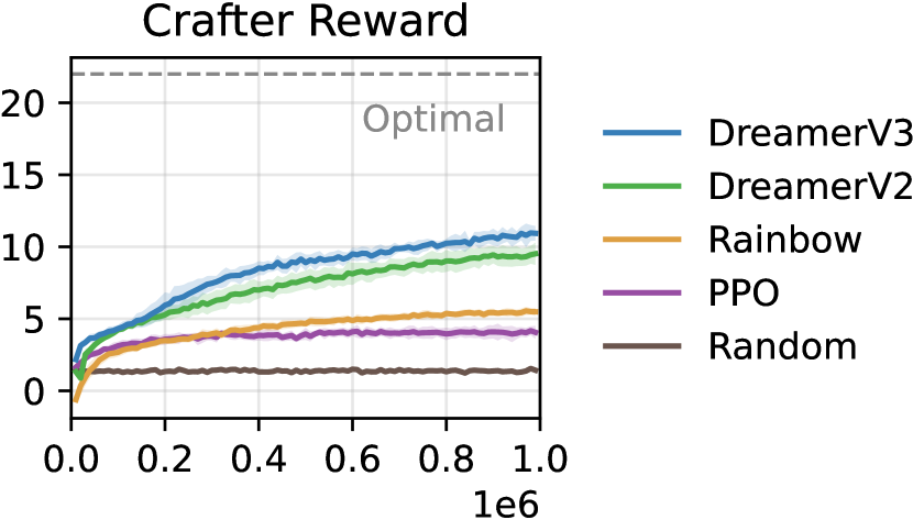
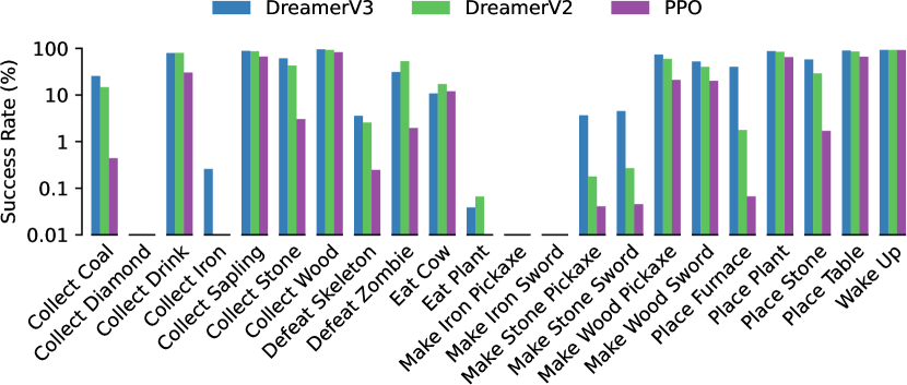
colspec = | L12em | C8em C8em |, row1 = font=,

Method Score Reward
Human Experts $50.5\pm 6.8\%$ $14.3\pm 2.3$
DreamerV3 $\mathbf{14.5\pm 1.6\%}$ $\mathbf{11.7\pm 1.9}$
LSTM-SPCNN $12.1\pm 0.8\%$ —
OC-SA $11.1\pm 0.7\%$ —
DreamerV2 $10.0\pm 1.2\%$ $\hphantom{0}9.0\pm 1.7$
PPO $\hphantom{0}4.6\pm 0.3\%$ $\hphantom{0}4.2\pm 1.2$
Rainbow $\hphantom{0}4.3\pm 0.2\%$ $\hphantom{0}6.0\pm 1.3$
Plan2Explore (Unsup) $\hphantom{0}2.1\pm 0.1\%$ $\hphantom{0}2.1\pm 1.5$
RND (Unsup) $\hphantom{0}2.0\pm 0.1\%$ $\hphantom{0}0.7\pm 1.3$
Random $\hphantom{0}1.6\pm 0.0\%$ $\hphantom{0}2.1\pm 1.3$

Table M.1: Crafter scores compared to previous algorithms and human performance.

Appendix N Proprioceptive Control Curves

Figure N.1: DMC scores for proprioceptive inputs with a budget of 500K frames.

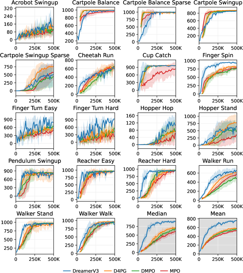
Appendix O Proprioceptive Control Scores

colspec = | L12em | C4em C4em C4em C4em C5em |, row1 = font=,

Task DDPG MPO DMPO D4PG DreamerV3
Environment Steps 500K 500K 500K 500K 500K
Acrobot Swingup 092.7 080.6 098.5 125.5 154.5
Cartpole Balance 996.2 958.4 998.5 998.8 990.5
Cartpole Balance Sparse 985.3 998.0 994.0 979.6 996.8
Cartpole Swingup 863.9 857.7 857.8 874.6 850.0
Cartpole Swingup Sparse 627.5 519.9 404.0 739.6 468.1
Cheetah Run 576.9 612.3 581.6 623.5 575.9
Cup Catch 905.5 800.6 965.8 968.3 958.2
Finger Spin 753.6 766.9 744.3 818.4 937.2
Finger Turn Easy 462.2 430.4 593.8 524.5 745.4
Finger Turn Hard 286.3 250.8 384.5 379.2 841.0
Hopper Hop 024.6 037.5 071.5 067.5 111.0
Hopper Stand 388.1 279.3 519.5 755.4 573.2
Pendulum Swingup 748.3 829.8 829.5 756.0 766.0
Reacher Easy 921.8 954.4 965.1 941.5 947.1
Reacher Hard 944.2 914.1 956.8 932.0 936.2
Walker Run 530.0 539.5 462.9 593.1 632.7
Walker Stand 967.4 960.4 971.6 935.2 956.9
Walker Walk 948.7 924.9 933.1 965.1 935.7
Median 751.0 783.7 786.9 787.2 845.5
Mean 667.9 650.9 685.2 721.0 743.1

Table O.1: DMC scores for proprioceptive inputs at 500K frames.

Appendix P Visual Control Curves

Figure P.1: DMC scores for image inputs with a budget of 1M frames.

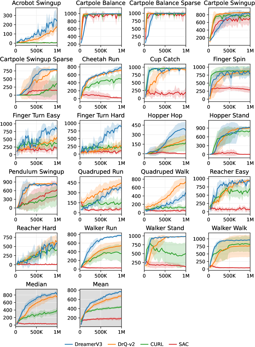
Appendix Q Visual Control Scores

colspec = | L12em | C5em C5em C5em C5em |, row1 = font=,

Task SAC CURL DrQ-v2 DreamerV3
Environment Steps 1M 1M 1M 1M
Acrobot Swingup 005.1 005.1 128.4 0210.0
Cartpole Balance 963.1 979.0 991.5 0996.4
Cartpole Balance Sparse 950.8 981.0 996.2 1000.0
Cartpole Swingup 692.1 762.7 858.9 0819.1
Cartpole Swingup Sparse 154.6 236.2 706.9 0792.9
Cheetah Run 027.2 474.3 691.0 0728.7
Cup Catch 163.9 965.5 931.8 0957.1
Finger Spin 312.2 877.1 846.7 0818.5
Finger Turn Easy 176.7 338.0 448.4 0787.7
Finger Turn Hard 070.5 215.6 220.0 0810.8
Hopper Hop 003.1 152.5 189.9 0369.6
Hopper Stand 005.2 786.8 893.0 0900.6
Pendulum Swingup 560.1 376.4 839.7 0806.3
Quadruped Run 050.5 141.5 407.0 0352.3
Quadruped Walk 049.7 123.7 660.3 0352.6
Reacher Easy 086.5 609.3 910.2 0898.9
Reacher Hard 009.1 400.2 572.9 0499.2
Walker Run 026.9 376.2 517.1 0757.8
Walker Stand 159.3 463.5 974.1 0976.7
Walker Walk 038.9 828.8 762.9 0955.8
Median 78.5 431.8 734.9 0808.5
Mean 225.3 504.7 677.4 0739.6

Table Q.1: DMC scores for visual inputs at 1M frames.

Appendix R Atari 100K Curves

Figure R.1: Atari training curves with a budget of 400K frames, amounting to 100K policy steps.

Appendix S Atari 100K Scores

colspec = | L6.5em | C3.5em C3.5em | C4.5em C4.5em C4.5em C4.5em C4.5em |, row1 = font=, stretch = 0.8,

Task Random Human SimPLe CURL SPR IRIS DreamerV3
Env Steps — — — 400K 400K 400K 400K
Alien 00228 07128 00617 0711 00842 00420 00959
Amidar 00006 01720 00074 0114 00180 00143 00139
Assault 00222 00742 00527 0501 00566 01524 00706
Asterix 00210 08503 01128 0567 00962 00854 00932
Bank Heist 00014 00753 00034 0065 00345 00053 00649
Battle Zone 02360 37188 04031 8998 14834 13074 12250
Boxing 00000 00012 00008 0001 00036 00070 00078
Breakout 00002 00030 00016 0003 00020 00084 00031
Chopper Com. 00811 07388 00979 0784 00946 01565 00420
Crazy Climber 10780 35829 62584 9154 36700 59324 97190
Demon Attack 00152 01971 00208 0646 00518 02034 00303
Freeway 00000 00030 00017 0028 00019 00031 00000
Frostbite 00065 04335 00237 1226 01171 00259 00909
Gopher 00258 02412 00597 0401 00661 02236 03730
Hero 01027 30826 02657 4988 05859 07037 11161
James Bond 00029 00303 00100 0331 00366 00463 00445
Kangaroo 00052 03035 00051 0740 03617 00838 04098
Krull 01598 02666 02205 3049 03682 06616 07782
Kung Fu Master 00258 22736 14862 8156 14783 21760 21420
Ms Pacman 00307 06952 01480 1064 01318 00999 01327
Pong 00–21 00015 00013 0–18 000–5 00015 00018
Private Eye 00025 69571 00035 0082 00086 00100 00882
Qbert 00164 13455 01289 0727 00866 00746 03405
Road Runner 00012 07845 05641 5006 12213 09615 15565
Seaquest 00068 42055 00683 0315 00558 00661 00618
Human Median 0% 100% 13% 09% 40% 029% 049%
Human Mean 0% 100% 33% 26% 62% 105% 112%

Table S.1: Atari scores at 400K environment frames, corresponding to 100k agent frames.

Appendix T Atari 100K Settings

colspec = | L10em | C4.5em C4.5em C4.5em C4.5em C4.5em C4.5em |, row1 = font=,

Setting SimPLe EfficientZero SPR IRIS TWM DreamerV3
Mean score 33 190 70 104 95 112
Median score 13 109 41 29 50 49
GPU days 10 1.2 0.2 7 0.8 0.5
Online planning — X — — — —
Data augmentation — — X — — —
Non-uniform replay — X X — X —
Separate hparams — — — X — —
Increased resolution — X X — — —
Uses life information — X X X X —
Uses early resets — X — X — —
Separate eval episodes X X X X X —

Table T.1: Algorithmic components, algorithmic components, and environment settings for the Atari 100k benchmark. GPU days are converted to V100 days by assuming P100 is twice as slow and A100 is twice as fast. EfficientZero achieves the highest scores but at the cost of complexity and changing the environment configuration. IRIS uses a separate exploration strength for Freeway.

Appendix U Atari 200M Curves

Figure U.1: Atari training curves with a budget of 200M frames.

Appendix V Atari 200M Scores

colspec = | L8.5em | C4em C4em C4em | C4.8em C4.8em C4.8em C4.8em |, row1 = font=, stretch = 0.8,

Task Random Gamer Record IQN Rainbow DreamerV2 DreamerV3
Environment Steps — — — 200M 200M 200M 200M
Alien 00229 07128 00251916 004926 003488 004083 0005404
Amidar 00006 01720 00104159 002315 002530 002531 0001141
Assault 00222 00742 00008647 004639 003302 023504 0018876
Asterix 00210 08503 01000000 010293 017534 075598 0039643
Asteroids 00719 47389 10506650 001578 001468 040120 0003829
Atlantis 12850 29028 10604840 890427 790051 996300 1439392
Bank Heist 00014 00753 00082058 001056 001079 001127 0001000
Battle Zone 02360 37188 00801000 040784 040194 042210 0035912
Beam Rider 00364 16926 00999999 007042 006232 018157 0020051
Berzerk 00124 02630 01057940 000644 000822 000807 0001245
Bowling 00023 00161 00000300 000039 000039 000049 0000158
Boxing 00000 00012 00000100 000098 000098 000091 0000099
Breakout 00002 00030 00000864 000080 000109 000293 0000300
Centipede 02091 12017 01301709 003735 006538 011816 0240525
Chopper Com. 00811 07388 00999999 009106 012388 002647 0005853
Crazy Climber 10780 35829 00219900 134761 145889 158278 0149986
Demon Attack 00152 01971 01556345 014558 016049 084408 0077084
Double Dunk 00–19 00–16 00000022 000021 000022 000018 0000023
Enduro 00000 00860 00009500 002207 002181 001775 0002289
Fishing Derby 00–92 00–39 00000071 000044 000042 000066 0000077
Freeway 00000 00030 00000038 000034 000034 000033 0000034
Frostbite 00065 04335 00454830 007866 008351 012091 0019991
Gopher 00258 02412 00355040 011469 010272 091249 0086759
Gravitar 00173 03351 00162850 001332 001263 003769 0000560
Hero 01027 30826 01000000 036216 046417 022003 0035359
Ice Hockey 00–11 00001 00000036 0000–5 0000–0 000026 0000027
Jamesbond 00007 00303 00045550 003294 001035 038514 0005123
Kangaroo 00052 03035 01424600 012562 012812 013899 0011597
Krull 01598 02666 00104100 008771 004238 055217 0020123
Kung Fu Master 00258 22736 01000000 030431 026489 063614 0068166
Montezuma Rev. 00000 04753 01219200 000495 000487 000079 0002512
Ms Pacman 00307 06952 00290090 005153 003913 005693 0011397
Name This Game 02292 08049 00025220 006718 009073 014879 0026439
Phoenix 00761 07243 04014440 005098 008355 047024 0090037
Pitfall 0–229 06464 00114000 000–17 000–12 0000–2 00000–0
Pong 00–21 00015 00000021 000020 000020 000020 0000020
Private Eye 00025 69571 00101800 004286 021341 002073 0005538
Qbert 00164 13455 02400000 016464 017625 114114 0137224
Riverraid 01338 17118 01000000 015250 020766 016791 0015758
Road Runner 00012 07845 02038100 058813 054704 249230 0078005
Robotank 00002 00012 00000076 000066 000065 000077 0000066
Seaquest 00068 42055 00999999 016819 009966 007341 0049547
Skiing –17098 –4337 000–3272 –11156 –28322 0–9813 00–9623
Solaris 01236 12327 00111420 001659 001829 001016 0002453
Space Invaders 00148 01669 00621535 004562 004112 002615 0006269
Star Gunner 00664 10250 00077400 079330 057289 010908 0008423
Tennis 00–24 000–8 00000021 000023 0000–0 000014 0000023
Time Pilot 03568 05229 00065300 011619 012041 036059 0068980
Tutankham 00011 00168 00005384 000248 000240 000265 0000285
Up N Down 00533 11693 00082840 063430 035440 651439 0502213
Venture 00000 01188 00038900 001314 001539 000000 0000000
Video Pinball 16257 17668 89218328 420509 450968 046282 0017416
Wizard Of Wor 00564 04756 00395300 005595 007869 012396 0036537
Yars Revenge 03093 54577 15000105 083990 045059 157285 0235402
Zaxxon 00032 09173 00083700 011047 014606 048620 0036626
Gamer Median 0% 100% 003716% 126% 147% 0219% 302%
Gamer Mean 0% 100% 126759% 890% 888% 1149% 920%
Record Mean 0% 012% 000100% 021% 017% 0044% 041%
Clip Record Mean 0% 012% 000100% 021% 017% 0028% 029%

Table V.1: Atari scores at 200M frames.

Appendix W Hyperparameters

colspec = | L15em | C6em | C10em |, row1 = font=,

Name Symbol Value
General
Replay capacity (FIFO) — $10^{6}\!\!$
Batch size $B$ 16
Batch length $T$ 64
Activation — $\operatorname{LayerNorm}+\operatorname{SiLU}$
World Model
Number of latents — 32
Classes per latent — 32
Reconstruction loss scale $\beta_{\mathrm{pred}}$ 1.0
Dynamics loss scale $\beta_{\mathrm{dyn}}$ 0.5
Representation loss scale $\beta_{\mathrm{rep}}$ 0.1
Learning rate — $10^{-4}$
Adam epsilon $\epsilon$ $10^{-8}$
Gradient clipping — 1000
Actor Critic
Imagination horizon $H$ 15
Discount horizon $1/(1-\gamma)$ 333
Return lambda $\lambda$ 0.95
Critic EMA decay — 0.98
Critic EMA regularizer — 1
Return normalization scale $S$ $\operatorname{Per}(R,95)-\operatorname{Per}(R,5)$
Return normalization limit $L$ 1
Return normalization decay — 0.99
Actor entropy scale $\eta$ $3\cdot 10^{-4}$
Learning rate — $3\cdot 10^{-5}$
Adam epsilon $\epsilon$ $10^{-5}$
Gradient clipping — 100

Table W.1: DreamerV3 hyper parameters. The same values are used across all benchmark suites, including proprioceptive and visual inputs, continuous and discrete actions, and 2D and 3D domains. We do not use any hyperparameter annealing, weight decay, or dropout.

References

- Silver et al. 2016 David Silver, Aja Huang, Chris J Maddison, Arthur Guez, Laurent Sifre, George Van Den Driessche, Julian Schrittwieser, Ioannis Antonoglou, Veda Panneershelvam, Marc Lanctot, et al. Mastering the game of go with deep neural networks and tree search. nature, 529(7587):484, 2016.
- OpenAI 2018 OpenAI. OpenAI Five. https://blog.openai.com/openai-five/, 2018.
- Andrychowicz et al. 2020 Marcin Andrychowicz, Anton Raichuk, Piotr Stańczyk, Manu Orsini, Sertan Girgin, Raphael Marinier, Léonard Hussenot, Matthieu Geist, Olivier Pietquin, Marcin Michalski, et al. What matters in on-policy reinforcement learning? a large-scale empirical study. arXiv preprint arXiv:2006.05990, 2020.
- Lillicrap et al. 2015 Timothy P Lillicrap, Jonathan J Hunt, Alexander Pritzel, Nicolas Heess, Tom Erez, Yuval Tassa, David Silver, and Daan Wierstra. Continuous control with deep reinforcement learning. arXiv preprint arXiv:1509.02971, 2015.
- Gu et al. 2016 Shixiang Gu, Timothy Lillicrap, Ilya Sutskever, and Sergey Levine. Continuous deep q-learning with model-based acceleration. In International conference on machine learning, pages 2829–2838. PMLR, 2016.
- Jaderberg et al. 2016 Max Jaderberg, Volodymyr Mnih, Wojciech Marian Czarnecki, Tom Schaul, Joel Z Leibo, David Silver, and Koray Kavukcuoglu. Reinforcement learning with unsupervised auxiliary tasks. arXiv preprint arXiv:1611.05397, 2016.
- Riedmiller et al. 2018 Martin Riedmiller, Roland Hafner, Thomas Lampe, Michael Neunert, Jonas Degrave, Tom Wiele, Vlad Mnih, Nicolas Heess, and Jost Tobias Springenberg. Learning by playing solving sparse reward tasks from scratch. In International conference on machine learning, pages 4344–4353. PMLR, 2018.
- Anand et al. 2019 Ankesh Anand, Evan Racah, Sherjil Ozair, Yoshua Bengio, Marc-Alexandre Côté, and R Devon Hjelm. Unsupervised state representation learning in atari. Advances in neural information processing systems, 32, 2019.
- Laskin et al. 2020 Misha Laskin, Kimin Lee, Adam Stooke, Lerrel Pinto, Pieter Abbeel, and Aravind Srinivas. Reinforcement learning with augmented data. Advances in Neural Information Processing Systems, 33:19884–19895, 2020.
- Mirchev et al. 2020 Atanas Mirchev, Baris Kayalibay, Patrick van der Smagt, and Justin Bayer. Variational state-space models for localisation and dense 3d mapping in 6 dof. arXiv preprint arXiv:2006.10178, 2020.
- Driess et al. 2022 Danny Driess, Ingmar Schubert, Pete Florence, Yunzhu Li, and Marc Toussaint. Reinforcement learning with neural radiance fields. arXiv preprint arXiv:2206.01634, 2022.
- Sutton 1991 Richard S Sutton. Dyna, an integrated architecture for learning, planning, and reacting. ACM SIGART Bulletin, 2(4):160–163, 1991.
- Ha and Schmidhuber 2018 David Ha and Jürgen Schmidhuber. World models. arXiv preprint arXiv:1803.10122, 2018.
- Hafner et al. 2018 Danijar Hafner, Timothy Lillicrap, Ian Fischer, Ruben Villegas, David Ha, Honglak Lee, and James Davidson. Learning latent dynamics for planning from pixels. arXiv preprint arXiv:1811.04551, 2018.
- Guss et al. 2019 William H Guss, Cayden Codel, Katja Hofmann, Brandon Houghton, Noboru Kuno, Stephanie Milani, Sharada Mohanty, Diego Perez Liebana, Ruslan Salakhutdinov, Nicholay Topin, et al. The minerl competition on sample efficient reinforcement learning using human priors. arXiv e-prints, pages arXiv–1904, 2019.
- Baker et al. 2022 Bowen Baker, Ilge Akkaya, Peter Zhokhov, Joost Huizinga, Jie Tang, Adrien Ecoffet, Brandon Houghton, Raul Sampedro, and Jeff Clune. Video pretraining (vpt): Learning to act by watching unlabeled online videos. arXiv preprint arXiv:2206.11795, 2022.
- Kanitscheider et al. 2021 Ingmar Kanitscheider, Joost Huizinga, David Farhi, William Hebgen Guss, Brandon Houghton, Raul Sampedro, Peter Zhokhov, Bowen Baker, Adrien Ecoffet, Jie Tang, et al. Multi-task curriculum learning in a complex, visual, hard-exploration domain: Minecraft. arXiv preprint arXiv:2106.14876, 2021.
- Mnih et al. 2015 Volodymyr Mnih, Koray Kavukcuoglu, David Silver, Andrei A Rusu, Joel Veness, Marc G Bellemare, Alex Graves, Martin Riedmiller, Andreas K Fidjeland, Georg Ostrovski, et al. Human-level control through deep reinforcement learning. Nature, 518(7540):529, 2015.
- Schulman et al. 2017 John Schulman, Filip Wolski, Prafulla Dhariwal, Alec Radford, and Oleg Klimov. Proximal policy optimization algorithms. arXiv preprint arXiv:1707.06347, 2017.
- Webber 2012 J Beau W Webber. A bi-symmetric log transformation for wide-range data. Measurement Science and Technology, 24(2):027001, 2012.
- Kapturowski et al. 2018 Steven Kapturowski, Georg Ostrovski, John Quan, Remi Munos, and Will Dabney. Recurrent experience replay in distributed reinforcement learning. In International conference on learning representations, 2018.
- Hessel et al. 2019 Matteo Hessel, Hubert Soyer, Lasse Espeholt, Wojciech Czarnecki, Simon Schmitt, and Hado van Hasselt. Multi-task deep reinforcement learning with popart. In Proceedings of the AAAI Conference on Artificial Intelligence, volume 33, pages 3796–3803, 2019.
- Hinton and Salakhutdinov 2006 Geoffrey E Hinton and Ruslan R Salakhutdinov. Reducing the dimensionality of data with neural networks. science, 313(5786):504–507, 2006.
- Kingma and Welling 2013 Diederik P Kingma and Max Welling. Auto-encoding variational bayes. arXiv preprint arXiv:1312.6114, 2013.
- LeCun et al. 1989 Yann LeCun, Bernhard Boser, John S Denker, Donnie Henderson, Richard E Howard, Wayne Hubbard, and Lawrence D Jackel. Backpropagation applied to handwritten zip code recognition. Neural computation, 1(4):541–551, 1989.
- Bengio et al. 2013 Yoshua Bengio, Nicholas Léonard, and Aaron Courville. Estimating or propagating gradients through stochastic neurons for conditional computation. arXiv preprint arXiv:1308.3432, 2013.
- Hafner et al. 2020 Danijar Hafner, Timothy Lillicrap, Mohammad Norouzi, and Jimmy Ba. Mastering atari with discrete world models. arXiv preprint arXiv:2010.02193, 2020.
- Kingma et al. 2016 Durk P Kingma, Tim Salimans, Rafal Jozefowicz, Xi Chen, Ilya Sutskever, and Max Welling. Improved variational inference with inverse autoregressive flow. Advances in neural information processing systems, 29, 2016.
- Vahdat and Kautz 2020 Arash Vahdat and Jan Kautz. Nvae: A deep hierarchical variational autoencoder. Advances in Neural Information Processing Systems, 33:19667–19679, 2020.
- Child 2020 Rewon Child. Very deep vaes generalize autoregressive models and can outperform them on images. arXiv preprint arXiv:2011.10650, 2020.
- Sutton and Barto 2018 Richard S Sutton and Andrew G Barto. Reinforcement learning: An introduction. MIT press, 2018.
- Schulman et al. 2015 John Schulman, Philipp Moritz, Sergey Levine, Michael Jordan, and Pieter Abbeel. High-dimensional continuous control using generalized advantage estimation. arXiv preprint arXiv:1506.02438, 2015.
- Bellemare et al. 2017 Marc G Bellemare, Will Dabney, and Rémi Munos. A distributional perspective on reinforcement learning. In International Conference on Machine Learning, pages 449–458. PMLR, 2017.
- Schrittwieser et al. 2019 Julian Schrittwieser, Ioannis Antonoglou, Thomas Hubert, Karen Simonyan, Laurent Sifre, Simon Schmitt, Arthur Guez, Edward Lockhart, Demis Hassabis, Thore Graepel, et al. Mastering atari, go, chess and shogi by planning with a learned model. arXiv preprint arXiv:1911.08265, 2019.
- Imani and White 2018 Ehsan Imani and Martha White. Improving regression performance with distributional losses. In International Conference on Machine Learning, pages 2157–2166. PMLR, 2018.
- van Hasselt et al. 2019 Hado van Hasselt, John Quan, Matteo Hessel, Zhongwen Xu, Diana Borsa, and André Barreto. General non-linear bellman equations. arXiv preprint arXiv:1907.03687, 2019.
- Williams and Peng 1991 Ronald J Williams and Jing Peng. Function optimization using connectionist reinforcement learning algorithms. Connection Science, 3(3):241–268, 1991.
- Haarnoja et al. 2018 Tuomas Haarnoja, Aurick Zhou, Pieter Abbeel, and Sergey Levine. Soft actor-critic: Off-policy maximum entropy deep reinforcement learning with a stochastic actor. arXiv preprint arXiv:1801.01290, 2018.
- Williams 1992 Ronald J Williams. Simple statistical gradient-following algorithms for connectionist reinforcement learning. Machine learning, 8(3-4):229–256, 1992.
- Tassa et al. 2018 Yuval Tassa, Yotam Doron, Alistair Muldal, Tom Erez, Yazhe Li, Diego de Las Casas, David Budden, Abbas Abdolmaleki, Josh Merel, Andrew Lefrancq, et al. Deepmind control suite. arXiv preprint arXiv:1801.00690, 2018.
- Barth-Maron et al. 2018 Gabriel Barth-Maron, Matthew W Hoffman, David Budden, Will Dabney, Dan Horgan, Alistair Muldal, Nicolas Heess, and Timothy Lillicrap. Distributed distributional deterministic policy gradients. arXiv preprint arXiv:1804.08617, 2018.
- Abdolmaleki et al. 2020 Abbas Abdolmaleki, Sandy Huang, Leonard Hasenclever, Michael Neunert, Francis Song, Martina Zambelli, Murilo Martins, Nicolas Heess, Raia Hadsell, and Martin Riedmiller. A distributional view on multi-objective policy optimization. In International Conference on Machine Learning, pages 11–22. PMLR, 2020.
- Abdolmaleki et al. 2018 Abbas Abdolmaleki, Jost Tobias Springenberg, Yuval Tassa, Remi Munos, Nicolas Heess, and Martin Riedmiller. Maximum a posteriori policy optimisation. arXiv preprint arXiv:1806.06920, 2018.
- Yarats et al. 2021 Denis Yarats, Rob Fergus, Alessandro Lazaric, and Lerrel Pinto. Mastering visual continuous control: Improved data-augmented reinforcement learning. arXiv preprint arXiv:2107.09645, 2021.
- Srinivas et al. 2020 Aravind Srinivas, Michael Laskin, and Pieter Abbeel. Curl: Contrastive unsupervised representations for reinforcement learning. arXiv preprint arXiv:2004.04136, 2020.
- Kaiser et al. 2019 Lukasz Kaiser, Mohammad Babaeizadeh, Piotr Milos, Blazej Osinski, Roy H Campbell, Konrad Czechowski, Dumitru Erhan, Chelsea Finn, Piotr Kozakowski, Sergey Levine, et al. Model-based reinforcement learning for atari. arXiv preprint arXiv:1903.00374, 2019.
- Ye et al. 2021 Weirui Ye, Shaohuai Liu, Thanard Kurutach, Pieter Abbeel, and Yang Gao. Mastering atari games with limited data. Advances in Neural Information Processing Systems, 34:25476–25488, 2021.
- Micheli et al. 2022 Vincent Micheli, Eloi Alonso, and François Fleuret. Transformers are sample efficient world models. arXiv preprint arXiv:2209.00588, 2022.
- Schwarzer et al. 2020 Max Schwarzer, Ankesh Anand, Rishab Goel, R Devon Hjelm, Aaron Courville, and Philip Bachman. Data-efficient reinforcement learning with self-predictive representations. arXiv preprint arXiv:2007.05929, 2020.
- Bellemare et al. 2013 Marc G Bellemare, Yavar Naddaf, Joel Veness, and Michael Bowling. The arcade learning environment: An evaluation platform for general agents. Journal of Artificial Intelligence Research, 47:253–279, 2013.
- Machado et al. 2018 Marlos C Machado, Marc G Bellemare, Erik Talvitie, Joel Veness, Matthew Hausknecht, and Michael Bowling. Revisiting the arcade learning environment: Evaluation protocols and open problems for general agents. Journal of Artificial Intelligence Research, 61:523–562, 2018.
- Hessel et al. 2018 Matteo Hessel, Joseph Modayil, Hado Van Hasselt, Tom Schaul, Georg Ostrovski, Will Dabney, Dan Horgan, Bilal Piot, Mohammad Azar, and David Silver. Rainbow: Combining improvements in deep reinforcement learning. In Thirty-Second AAAI Conference on Artificial Intelligence, 2018.
- Dabney et al. 2018 Will Dabney, Georg Ostrovski, David Silver, and Rémi Munos. Implicit quantile networks for distributional reinforcement learning. In International conference on machine learning, pages 1096–1105. PMLR, 2018.
- Osband et al. 2019 Ian Osband, Yotam Doron, Matteo Hessel, John Aslanides, Eren Sezener, Andre Saraiva, Katrina McKinney, Tor Lattimore, Csaba Szepesvari, Satinder Singh, et al. Behaviour suite for reinforcement learning. arXiv preprint arXiv:1908.03568, 2019.
- Osband et al. 2016 Ian Osband, Charles Blundell, Alexander Pritzel, and Benjamin Van Roy. Deep exploration via bootstrapped DQN. In Advances in neural information processing systems, pages 4026–4034, 2016.
- Hessel et al. 2021 Matteo Hessel, Ivo Danihelka, Fabio Viola, Arthur Guez, Simon Schmitt, Laurent Sifre, Theophane Weber, David Silver, and Hado Van Hasselt. Muesli: Combining improvements in policy optimization. In International Conference on Machine Learning, pages 4214–4226. PMLR, 2021.
- Hafner 2021 Danijar Hafner. Benchmarking the spectrum of agent capabilities. arXiv preprint arXiv:2109.06780, 2021.
- Stanić et al. 2022 Aleksandar Stanić, Yujin Tang, David Ha, and Jürgen Schmidhuber. Learning to generalize with object-centric agents in the open world survival game crafter. arXiv preprint arXiv:2208.03374, 2022.
- Beattie et al. 2016 Charles Beattie, Joel Z Leibo, Denis Teplyashin, Tom Ward, Marcus Wainwright, Heinrich Küttler, Andrew Lefrancq, Simon Green, Víctor Valdés, Amir Sadik, et al. Deepmind lab. arXiv preprint arXiv:1612.03801, 2016.
- Espeholt et al. 2018 Lasse Espeholt, Hubert Soyer, Remi Munos, Karen Simonyan, Volodymir Mnih, Tom Ward, Yotam Doron, Vlad Firoiu, Tim Harley, Iain Dunning, et al. Impala: Scalable distributed deep-rl with importance weighted actor-learner architectures. arXiv preprint arXiv:1802.01561, 2018.
- Yarats et al. 2019 Denis Yarats, Amy Zhang, Ilya Kostrikov, Brandon Amos, Joelle Pineau, and Rob Fergus. Improving sample efficiency in model-free reinforcement learning from images. arXiv preprint arXiv:1910.01741, 2019.
- Reed et al. 2022 Scott Reed, Konrad Zolna, Emilio Parisotto, Sergio Gomez Colmenarejo, Alexander Novikov, Gabriel Barth-Maron, Mai Gimenez, Yury Sulsky, Jackie Kay, Jost Tobias Springenberg, et al. A generalist agent. arXiv preprint arXiv:2205.06175, 2022.
- Johnson et al. 2016 Matthew Johnson, Katja Hofmann, Tim Hutton, and David Bignell. The malmo platform for artificial intelligence experimentation. In IJCAI, pages 4246–4247. Citeseer, 2016.
- Fan et al. 2022 Linxi Fan, Guanzhi Wang, Yunfan Jiang, Ajay Mandlekar, Yuncong Yang, Haoyi Zhu, Andrew Tang, De-An Huang, Yuke Zhu, and Anima Anandkumar. Minedojo: Building open-ended embodied agents with internet-scale knowledge. arXiv preprint arXiv:2206.08853, 2022.
- Hafner et al. 2019 Danijar Hafner, Timothy Lillicrap, Jimmy Ba, and Mohammad Norouzi. Dream to control: Learning behaviors by latent imagination. arXiv preprint arXiv:1912.01603, 2019.
- Rezende and Viola 2018 Danilo Jimenez Rezende and Fabio Viola. Taming vaes. arXiv preprint arXiv:1810.00597, 2018.
- Hilton et al. 2021 Jacob Hilton, Karl Cobbe, and John Schulman. Batch size-invariance for policy optimization. arXiv preprint arXiv:2110.00641, 2021.
- Wiering 1999 Marco A Wiering. Explorations in efficient reinforcement learning. PhD thesis, University of Amsterdam, 1999.
- Gruslys et al. 2017 Audrunas Gruslys, Will Dabney, Mohammad Gheshlaghi Azar, Bilal Piot, Marc Bellemare, and Remi Munos. The reactor: A fast and sample-efficient actor-critic agent for reinforcement learning. arXiv preprint arXiv:1704.04651, 2017.
- Ba et al. 2016 Jimmy Lei Ba, Jamie Ryan Kiros, and Geoffrey E Hinton. Layer normalization. arXiv preprint arXiv:1607.06450, 2016.
- Hendrycks and Gimpel 2016 Dan Hendrycks and Kevin Gimpel. Gaussian error linear units (gelus). arXiv preprint arXiv:1606.08415, 2016.
- Hafner et al. 2022 Danijar Hafner, Kuang-Huei Lee, Ian Fischer, and Pieter Abbeel. Deep hierarchical planning from pixels. arXiv preprint arXiv:2206.04114, 2022.
- Higgins et al. 2016 Irina Higgins, Loic Matthey, Arka Pal, Christopher Burgess, Xavier Glorot, Matthew Botvinick, Shakir Mohamed, and Alexander Lerchner. beta-vae: Learning basic visual concepts with a constrained variational framework. In International Conference on Learning Representations, 2016.
- Park et al. 2021 Seohong Park, Jaekyeom Kim, and Gunhee Kim. Time discretization-invariant safe action repetition for policy gradient methods. Advances in Neural Information Processing Systems, 34:267–279, 2021.
Appendices
psection[2.3em]\contentslabel2.3em\contentspage \startcontents[sections] \printcontents[sections]p1