A CAD System for Colorectal Cancer from WSI: A Clinically Validated Interpretable ML-based Prototype

Abstract

The integration of Artificial Intelligence (AI) and Digital Pathology has been increasing over the past years. Nowadays, applications of deep learning (DL) methods to diagnose cancer from whole-slide images (WSI) are, more than ever, a reality within different research groups. Nonetheless, the development of these systems was limited by a myriad of constraints regarding the lack of training samples, the scaling difficulties, the opaqueness of DL methods, and, more importantly, the lack of clinical validation. As such, we propose a system designed specifically for the diagnosis of colorectal samples. The construction of such a system consisted of four stages: (1) a careful data collection and annotation process, which resulted in one of the largest WSI colorectal samples datasets; (2) the design of an interpretable mixed-supervision scheme to leverage the domain knowledge introduced by pathologists through spatial annotations; (3) the development of an effective sampling approach based on the expected severeness of each tile, which decreased the computation cost by a factor of almost 6x; (4) the creation of a prototype that integrates the full set of features of the model to be evaluated in clinical practice. During these stages, the proposed method was evaluated in four separate test sets, two of them are external and completely independent. On the largest of those sets, the proposed approach achieved an accuracy of 93.44%. DL for colorectal samples is a few steps closer to stop being research exclusive and to become fully integrated in clinical practice.

[inesc]organization=Institute for Systems and Computer Engineering, Technology and Science (INESC TEC), addressline=R. Dr. Roberto Frias, city=Porto, postcode=4200-465, state=Porto, country=Portugal

[feup]organization=Faculty of Engineering, University of Porto (FEUP), addressline=R. Dr. Roberto Frias, city=Porto, postcode=4200-465, state=Porto, country=Portugal [imp]organization=IMP Diagnostics, addressline=Praca do Bom Sucesso, 61, sala 809, city=Porto, postcode=4150-146, state=Porto, country=Portugal

[ipo1]organization=Cancer Biology and Epigenetics Group, IPO-Porto, addressline=R. Dr. António Bernardino de Almeida 865, city=Porto, postcode=4200-072, state=Porto, country=Portugal [ipo2]organization=Department of Pathology, IPO-Porto, addressline=R. Dr. António Bernardino de Almeida 865, city=Porto, postcode=4200-072, state=Porto, country=Portugal [icbas]organization=School of Medicine and Biomedical Sciences, University of Porto (ICBAS), addressline=R. Jorge de Viterbo Ferreira 228, city=Porto, postcode=4050-313, state=Porto, country=Portugal

[bern]organization=Institute of Pathology, University of Bern, addressline=Uni Bern, Murtenstrasse 31, city=Bern, postcode=3008, state=Bern, country=Switzerland

1 Introduction

Colorectal cancer (CRC) incidence and mortality are increasing, and it is estimated that they will keep growing at least until 2040 [1], according to estimations of the International Agency for Research on Cancer. Nowadays, it is the third most incident (10.7% of all cancer diagnoses) and the second most deadly type of cancer [1]. Due to the effect of lifestyle, genetics, environmental factors and an increase in life expectancy, the current increase in world wealth and the adoption of western lifestyles further advocates for an increase in the capabilities to perform more CRC evaluations for potential diagnosis [2, 3]. Despite the pessimist predictions for an increase in the incidence, CRC is preventable and curable when detected in its earlier stages. Thus, effective screening through medical examination, imaging techniques and colonoscopy are of utmost importance [4, 5].

Despite the CRC detection capabilities shown by imaging techniques, the diagnosis of cancer is always based on the pathologist’s evaluation of biopsies/surgical specimen samples. The stratification of neoplasia development stages consists of non-neoplastic (NNeo), low-grade dysplasia (LGD), high-grade dysplasia (HGD, including intramucosal carcinomas), and invasive carcinomas, from the initial to the latest stage of cancer progression, respectively. In spite of the inherent subjectivity of the dysplasia grading system [6], recent guidelines from the European Society of Gastrointestinal Endoscopy (ESGE), as well as those from the US multi-society task force on CRC, consistently recommend shorter surveillance intervals for patients with polyps with high-grade dysplasia, regardless of their dimension [5, 7]. Hence, grading dysplasia is still routinely performed by pathologists worldwide when assessing colorectal tissue samples.

Private datasets of digitised slides are becoming widely available, in the form of whole-slide images (WSI), with an increase in the adoption of digital workflows [8, 9, 10]. Despite the burden of the additional scanning step, WSI eases the revision of old cases, data sharing and quick peer-review [11, 12]. It has also created several research opportunities within the computer vision domain, especially due to the complexity of the problem and the high dimensions of WSI [13, 14, 15, 16]. As such, robust and high-performance systems can be valuable assets to the digital workflow of a laboratory, especially if they are transparent and interpretable [11, 12]. However, some limitations still affect the applicability of such solutions in practice [17].

The majority of the works on CRC diagnosis direct their focus towards the classification of cropped regions of interest, or small tiles, instead of tackling the challenging task of diagnosing the entire WSI [18, 19, 17, 20]. Notwithstanding, some authors already presented methods to assess the grading of the complete slide of colorectal samples. In 2020, Iizuka et al. [21] used a recurrent neural network (RNN) to aggregate the predictions of individual tiles processed by an Inception-v3 network into non-neoplastic, adenoma (AD) and adenocarcinoma (ADC). Due to the large dimensions of WSI related to their pyramidal format (with several magnification levels) [22], usually over 50,000 $\times$ 50,000 pixels, it is usual to use a scheme consisting of a grid of tiles. This scheme permits the acceleration of the processing steps since the tiles are small enough to fit in the memory of the graphics processing units (GPU), popular units for the training of deep learning (DL). Wei et al. [23] studied the usage of an ensemble of five distinct ResNet networks, in order to distinguish the types of CRC adenomas H&E stained slides. Song et al. [24] experimented with a modified DeepLab-v2 network for tile classification, and proposed pixel probability thresholding to detect CRC adenomas. Both Xu et al. [25] and Wang et al. [26, 27] looked into the performance of the Inception-v3 architecture to detect CRC, with the latter also retrieving a cluster-based slide classification and a map of predictions. The MuSTMIL [28] method, classifieds five colon-tissue findings: normal glands, hyperplastic polyps, low-grade dysplasias, high-grade dysplasias and carcinomas. This classification originates from a multitask architecture that leverages several levels of magnification of a slide. Ho et al. [29] extended the experiments with multitask learning, but instead of leveraging the magnification, its model aims to jointly segment glands, detect tumour areas and sort the slides into low-risk (benign, inflammation or reactive changes) and high-risk (adenocarcinoma or dysplasia) categories. The architecture of this model is considerably more complex, with regard to the number of parameters, and is known as Faster-RCNN with a ResNet-101 backbone network for the segmentation task. Further to this task, a gradient-boosted decision tree completes the pipeline that results in the final grade.

As stated in the previous paragraph, recent state-of-the-art computer-aided diagnosis systems are based on deep learning approaches. These systems rely on large volumes of data to learn how to perform a particular task. Increasing the complexity of the task often demands an increase in the data available. Collecting this data is expensive and tedious due to the annotation complexity and the need for expert knowledge. Despite recent publications that present approaches using large volumes of data to train CAD systems, the majority do not publicly release the data used. To reverse this trend, the novel and completely anonymised dataset introduced in this document will have the majority of the available slides publicly released. This dataset contains, approximately, 10500 high-quality slides. The available slides originate one of the largest colorectal samples (CRS) datasets to be made publicly available. This high volume of data, in addition to the massive resolution of the images, creates a significant bottleneck of deep learning approaches that extract patches from the whole slide. Hence, we introduce an efficient sampling approach that is performed once without sacrificing prediction performance. The proposed sampling leverages knowledge learnt from the data to create a proxy that reduces the rate of important information discarded, when compared to random sampling. Due to the cost of annotating the entire dataset, it is only annotated for a portion at the pixel level, while the remaining portion is labelled for a portion at the slide level. To leverage these two levels of supervision, we propose a mixed supervision training scheme.

One other increasingly relevant issue with current research is the lack of external validation. It is not uncommon to observe models that perform extremely well on a test set collected from the same data distribution used to train, but fail on samples from other laboratories or scanners. Hence, we validate our proposed model in two different external datasets that vary in quality, country of origin and laboratory. While the results on a similar dataset show the performance of the model if implemented in the institution that collects that data, the test on external samples indicates its capabilities to be deployed in other scenarios.

In order to bring this CAD system into production, and to infer its capabilities within clinical practice, we developed a prototype that has been used by pathologists in clinical practice. We further collected information on the misdiagnoses and the pathologists’ feedback. Since it is expected that the model indicates some rationale behind its predictions, we developed a visual approach to explain the decision and guide pathologists’ focus toward more aggressive areas. This mechanism increased the acceptance of the algorithm in clinical practice, and its usefulness. When collected from routine the slides can be digitised with duplicated tissue areas, known as fragments, which might be of lower quality. Hence, the workflow for the automatic diagnostic also included an automatic fragment detection and counting system [30]. Moreover, it was possible to utilize this prototype to do the second round of labelling based on the test set prediction given by the model. This second round led to the correction of certain labels (that the model predicted correctly and were mislabeled by the expert pathologist) and insights regarding the areas where the model has to be improved.

To summarise, in this paper we propose a novel dataset with more than thirteen million tiles, a sampling approach to reduce the difficulty of using large datasets, a deep learning model that is trained with mixed supervision, evaluated on two external datasets, and incorporated in a prototype that provides a simple integration in clinical practice and visual explanations of the model’s predictions. This way, we come a step closer to making CAD tools a reality for colorectal diagnosis.

2 Methods

In this section, after defining the problem at hand, we introduce the proposed dataset used to train, validate and test the model, the external datasets to evaluate the generalisation capabilities of the model and the pre-processing pipeline. Afterwards, we describe in detail the methodology followed to create the deep learning model and to design the experiments. Finally, we also detail the clinical assessment and evaluation of the model.

2.1 Problem definition

Digitised colorectal cancer histological samples have large dimensions, which are far larger than the dimensions of traditional images used in medical or general computer vision problems. Labelling such images is expensive and highly dependent on the availability of expert knowledge. It limits the availability of whole slide images, and, in scenarios where these are available, meaningful annotations are usually lacking. On the other hand, it is easier to label the dataset at the slide level. The inclusion of detailed spatial annotations on approximately 10% of the dataset has been shown to positively impact the performance of deep learning algorithms [17, 31].

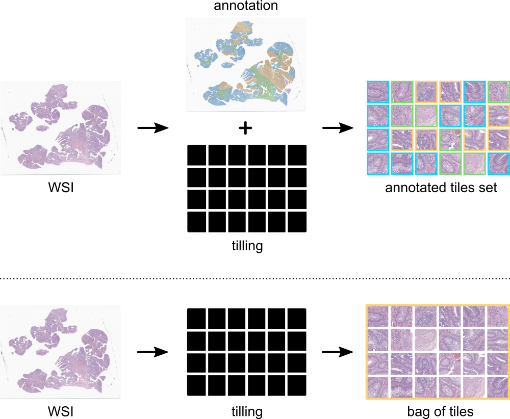
Figure 1: Problem definition as a fully supervised task (on top), and as a weakly-supervised task (bottom).

To fully leverage the potential of spatial and slide labels, we propose a deep learning pipeline, based on previous approaches [17, 31], using mixed supervision. Each slide, ${\mathcal{S}}$ is composed of a set of tiles $\mathcal{T}_{s,n}$, where $s$ represents the index of the slide and $n\in\{1,\cdots,n_{s}\}$ the tile number. Furthermore, there is an inherent order in the grading used to classify the input into one of the $C^{(k)}$ classes, which represents a variation in severity. For fully supervised learning, only strongly annotated slides are useful, and for those, the label of each tile $C_{s,n}$ is known. The remaining slides are deprived of these detailed labels, hence, they can only be leveraged by training algorithms with weakly supervision. To be used by these algorithms, the weakly annotated slides have only a single label for the entire bag (set) of tiles, as seen in Figure 1. Following the order of the labels and the clinical knowledge, we assume that the predicted slide label $C_{s}$ is the most severe case of the tile labels:

$C_{s}=\max_{n}\{C_{s,n}\}.$

In other words, if there is at least one tile classified as containing high-grade dysplasia, then the entire slide that contains the tile is classified accordingly. On the other end of the spectrum, if the worst tile is classified as non-neoplastic, then it is assumed that there is no dysplasia in the entire set of tiles. This is a generalisation of multiple-instance learning (MIL) to an ordinal classification problem, as proposed by Oliveira et al. [17].

2.2 Datasets

The spectrum of large-scale CRC/CRS datasets is slowly increasing due to the contributions of several researchers. Two datasets that have been recently introduced in the literature are the CRS1K [17] and CRS4K [31] datasets. Since the latter is an extension of the former with roughly four times more slides, it will be the baseline dataset for the remaining of this document. Moreover, we further extend these with the CRS10K dataset, which contains 9.26x and 2.36x more slides than CRS1K and CRS4K, respectively. Similarly, the number of tiles is multiplied by a factor of 12.2 and 2.58 (Table 1). This volume of slides is translated into an increase in the flexibility to design experiments and infer the robustness of the model. Thus, the inclusion of a test set separated from the validation set is now facilitated.

The set is composed of colorectal biopsies and polypectomies (excluding surgical specimens). Following the same annotation process as the previous datasets, CRS10K slides are labelled according to three main categories: non-neoplastic (NNeo), low-grade lesions (LG), and high-grade lesions (HG). The first, contains normal colorectal mucosa, hyperplasia and non-specific inflammation. LG lesions categorise conventional adenomas with low-grade dysplasia. Finally, HG lesions are composed of adenomas with high-grade dysplasia (including intra-mucosal carcinomas) and invasive adenocarcinomas. In order to avoid diversions from the main goal, slides with suspicion of known history of inflammatory bowel disease/infection, serrated lesions or other polyp types were not included in the dataset.

The slides, retrieved from an archive of previous cases, were digitised with Leica GT450 WSI scanners, at 40$\times$ magnification. The cases were initially seen and classified (labelled) by one of three pathologists. The pathologist revised and classified the slides, and then compared them with the initial report diagnosis (which served as a second-grader). If there was a match between both, no further steps were taken. In discordant cases, a third pathologist served as a tie-breaker. Roughly 9% of the dataset (967 slides and over a million tiles) were manually annotated by a pathologist and rechecked by the other, in turn, using the Sedeen Viewer software [32]. For complex cases, or when the agreement for a joint decision could not be reached, a third pathologist reevaluated the annotation.

The CRS10K dataset was divided into train, validation and test sets. The first includes all the strongly annotated slides and other slides randomly selected. Whereas the second is composed of only non-annotated slides. Finally, the test set was selected from the new data added to extend the previous datasets. Thus, it is completely separated from the training and validation sets of previous works. The test set, will be publicly available, so that future research can directly compare their results and use that set as a benchmark.

Table 1: Dataset summary, with the number of slides (annotated samples are detailed in parentheses) and tiles distributed by class for all the datasets used in this study.

		NNeo	LG	HG	Total
	# slides	300 (6)	552 (35)	281 (59)	1133 (100)
CRS1K dataset [17]	# annotated tiles	49,640	77,946	83,649	211,235
	# non-annotated tiles	-	-	-	1,111,361
	# slides	663 (12)	2394 (207)	1376 (181)	4433 (400)
CRS4K dataset [31]	# annotated tiles	145,898	196,116	163,603	505,617
	# non-annotated tiles	-	-	-	5,265,362
	# slides	1740 (12)	5387 (534)	3369 (421)	10,496 (967)
CRS10K dataset	# annotated tiles	338,979	371,587	341,268	1,051,834
	# non-annotated tiles	-	-	-	13,571,871
CRS Prototype	# slides	28	44	28	100
	# non-annotated tiles	-	-	-	244,160
PAIP [33]	# slides	-	-	100	100
	# non-annotated tiles	-	-	-	97,392
TCGA [34]	# slides	1	1	230	232
	# non-annotated tiles	-	-	-	1,568,584

Furthermore, as detailed in the following sections, this work comprises the development of a fully-functional prototype to be used in clinical practice. Leveraging this prototype, it was possible to further collect a new set with 100 slides. It differs from the CRS10K dataset, in the sense that they were not carefully selected from the archives. Instead, these cases were actively collected from the current year’s routine exams. We argue that this might better reflect the real-world data distribution. Hence, we introduce this set as a distinct dataset to evaluate the robustness of the presented methodology. Differently from the datasets discussed below, the CRS Prototype dataset has a more balanced distribution of the slide labels. Although it is useful in practice, the usage of the fragment counting and selection algorithm for the evaluation could potentiate the propagation of errors from one system to another. Thus, in this evaluation, we did not use the fragment selection algorithm, and as shown in Table 1, the number of tiles per slide doubles when compared to CRS10K, which had its fragments carefully selected.

To evaluate the domain generalisation of the proposed approach, two external datasets were used. We evaluate the proposed approaches on two external datasets publicly available. The first dataset is composed of samples of the TCGA-COAD [35] and TCGA-READ [36] collections from The Cancer Imaging Archive [34], which are composed in general by resection samples (in contrast to our dataset, composed only of biopsies and polypectomies). Samples containing pen markers, large air bubbles over tissue, tissue folds, and other artefacts affecting large areas of the slide were excluded. The final selection includes 232 whole-slide images reviewed and validated by the same pathologists that reviewed the in-house datasets. 230 of those samples were diagnosed as high-grade lesions, whereas the remaining two have been diagnosed as low-grade and non-neoplastic. For this dataset, the specific model of the scanner used to digitise the images is unknown, but the file type (”.svs”) matches the file type of the training data. The second external dataset used to evaluate the model contains 100H&E slides from the Pathology AI Platform [33] colorectal cohort, which contains all the cases with a more superficial sampling of the lesion, for a better comparison with our datasets. All the whole slide images in this dataset were digitised with an Aperio AT2 at 20X magnification. Finally, the pathologists’ team followed the same guidelines to review and validate all the WSI, which were all classified as high-grade lesions. It is interesting to note that while the PAIP contains significantly fewer tiles per slide, around 973, than the CRS10K dataset, around 1293, the TCGA dataset shows the largest amount of tissue per slide with an average of 6761 tiles as seen in Table 1.

2.3 Data pre-processing

H&E slides are composed of two distinct elements, white background and colourful tissue. Since the former is not meaningful for the diagnostic, the pre-processing of these slides incorporates an automatic tissue segmentation with Otsu’s thresholding [37] on the saturation (S) channel of the HSV colour space, resulting in a separation between the tissue regions and the background. The result of this step, which receives as input a $32\times$ downsampled slide, is the mask used for the following steps. Leveraging this previous output, tiles with a dimension of $512\times 512$ pixels (Figure 2) were extracted from the original slide (without any downsampling) at its maximum magnification (40$\times$), if they did not include any portion of background (i.e. a 100% tissue threshold was used). Following previous experiments in the literature, our empirical assessment, and the confirmation that smaller tiles would significantly increase the number of tiles and the complexity of the task, $512\times 512$ was chosen as the tile size. Moreover, it is believed that $512\times 512$ is the smallest tile size that still incorporates enough information to make a good diagnostic with the possibility of visually explaining the decision [17]. The selected threshold of 100% further reduces the number of tiles by not including the tissue at the edges and decreases the complexity of the task, since the model does not see the background at any moment. Due to tissue variations in different images, there is also a different number of tiles extracted per image.

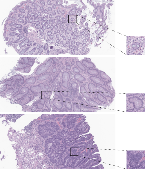
Figure 2: Examples of regions with and a sample tile with $512\times 512$ pixels (40$\times$ magnification), representing each class: non-neoplastic (on top), low-grade dysplasia (on the middle) and high-grade dysplasia (on the bottom).

2.4 Methodology

The massive size of images, which translates to thousands of tiles per image, allied to a large number of samples in the CRS10K dataset, bottlenecks the training of weakly-supervised models based on multiple instance learning (MIL). Hence, in this document, we propose a mix-supervision approach with self-contained tile sampling to diagnose colorectal cancer samples from whole-slide images. This subsection comprises the methodology, which includes supervised training, sampling and weakly-supervised learning.

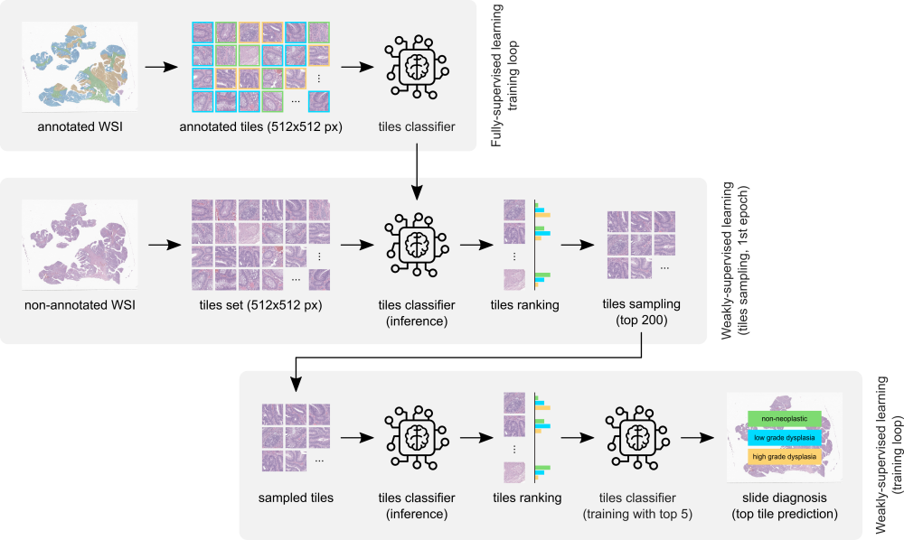
Figure 3: Overall scheme of the proposed methodology containing the mix-supervision framework that is responsible for diagnosing colorectal samples from WSI.

2.4.1 Supervised Training

As mentioned in previous sections, spatial annotations are rare in large quantities. However, these include domain information, given by the expert annotator, concerning the most meaningful areas and what are the most and less severe tiles. Thus, they can facilitate the initial optimisation of a deep neural network. As shown in the literature, there has been some research on the impact of starting the training with a few iterations of fully-supervised training [17, 38]. We further explore this in three different ways. First, we have 967 annotated slides resulting in more than one million annotated tiles for supervised training. Secondly, attending to the size of our dataset and the need for a stronger initial supervised training, the models are trained for 50 epochs, and their performance was monitored over specific checkpoint epochs. Finally, we explore this pre-trained model as the main tool to sample useful tiles for the weakly-supervised task.

2.4.2 Tile Sampling

Our scenario presents a particularly difficult condition for scaling the training data. First, let’s consider the structure of the data, which consists of, on average, more than one thousand tiles per slide. Within this set of tiles, some tiles provide meaningful value for the prediction, and others do not add extra information. In other words, for the CRS10K dataset, the extensive, lengthy, time and energy-consuming process of going through 13 million tiles every epoch can be avoided, and as result, these models can be trained for more epochs. Nowadays, there is an increasing concern regarding energy and electricity consumption. Thus, these concerns, together with the sustainability goals, further support the importance of more efficient training processes.

Let $\mathcal{T}$ be the original set of tiles, and $\mathcal{T}_{s}$ be the original set of tiles from the slide $s$, the former is composed by a union of the latter of all the slides (Eq. 1). We propose to map $\mathcal{T}$ to a smaller set of tiles $\mathcal{M}$ without affecting the overall performance and behaviour of the trained algorithm.

$$\mathcal{T}=\bigcup\limits_{s=1}^{S}\mathcal{T}_{s}$$ (1)

The model trained in a fully supervised task, previously described, provides a good estimation of the utility of each tile. Hence, we utilise the function ($\Phi$) learned by the model to compute the predicted severity of each tile. As will be shown below, the weakly-supervised method utilises only the five most severe tiles per slide to train in each epoch. As such, we select M tiles per slide (M=200 in our experimental setup) utilising a Top-k function (with k set to 200) to be retained for the weakly-supervised training. As indicated by the results presented in the following sections, the value of M was selected in accordance with a trade-off between information lost and training time. This is formalised in Eq. 2.

$$\mathcal{M}_{s}=\textrm{Top-k}(\Phi(\mathcal{T}_{s}))$$ (2)

For instance, in the CRS10K dataset, the total number of tiles after sampling would be at most 2,099,200, which represents a reduction of 6.46$\times$ when compared to the total number of slides. Despite this upper bound on the number of tiles, there are WSI samples that contain less than M tiles, and as such, they remain unsampled and the actual total number of tiles after sampling is potentially lower. During the evaluation and test time, there is no sampling.

We conducted extensive studies on the performance of our methodology, without sampling, with sampling on the training data, and with sampling on training and validation. The results on the CRS4K dataset validate our proposal. The number of selected tiles considers a trade-off between computational cost and information potentially lost, and for that reason, it is the success of empirical optimization.

2.4.3 Weakly-Supervised Learning

The weakly-supervised learning approach designed for our methodology follows the same principles of recent work [31]. It is divided into two distinct stages, tile severity analysis and training. The former utilises the pre-trained model to evaluate the severity of every tile in a set of tiles. In the first epoch, $\mathcal{T}$, the set of all the tiles in the complete dataset is used. This is possible since the model used to assess the severity in this epoch is the same one used for sampling. Hence, both tasks are integrated with the initial epoch. The following epochs utilise the sampled tile set $\mathcal{M}$ instead of the original set. This overall structure is represented in Figure 3.

The link between both stages is guided by a slide-wise tile ranking approach based on the expected severity. For tile $\mathcal{T}_{s,n}$, the expected severity is defined as

$$\mathbb{E}(\hat{C}_{s,n})=\sum_{i=1}^{K}i\times p\left(\hat{C}_{s,n}=C^{(i)}\right)$$ (3)

where $\hat{C}_{s,n}$ is a random variable on the set of possible class labels $\{C^{(1)},\cdots,C^{(K)}\}$ and $p\left(\hat{C}_{s,n}=C^{(i)}\right)$ are the $K$ output values of the neural network. After this analysis, the five most severe tiles are selected for training. The number of selected tiles was chosen in accordance with previous studies [31]. These five tiles per slide are used to train the proposed model for one more epoch. Each epoch is composed of both stages, which means that the tiles used for training vary across epochs. The slide label is used as the ground truth of all five tiles of that same slide used for network optimisation. For validation and evaluation, only the most severe tile is used for diagnostics. Although it might lead to an increase in false positives, it shall significantly reduce false negatives. Furthermore, we argue that increasing the variability and quantity of data available leads to a better balance between the reduction of these two types of errors.

2.5 Confidence Interval

In order to quantify the uncertainty of a result, it is common to compute the 95 percent confidence interval. In this way, two different models can be easily understood and compared based on the overlap of their confidence intervals. The standard approach to calculating these intervals requires several runs of a single experiment. As we increase the number of runs, our interval becomes narrower. However, this procedure is impractical for the computationally intensive experiments presented in this document. Hence, we use an independent test set to approximate the confidence interval as a Gaussian function [39]. To do so, we compute the standard error ($SE$) of an evaluation metric $m$, which is dependent on the number of samples ($n$), as seen in Equation 4.

$$SE=\sqrt{\frac{1}{n}\times m\times(1-m)}$$ (4)

For the SE computation to be mathematically correct, the metric $m$ must originate from a set of Bernoulli trials. In other words, if each prediction is considered a Bernoulli trial, then the metric should classify them as correct or incorrect. The number of correct samples is then given by a Binomial distribution $X\sim(n,p)$, where $p$ is the probability of correctly predicting a label, and $n$ is the number of samples. For instance, the accuracy is a metric that fits all these constraints.

Following the definition and the properties of a Normal distribution, we compute the number of standard deviations ($z$), known as a standard score, that can be translated to the desired confidence ($c$) set to 95% of the area under a normal distribution. This is a well-studied value, which is approximately $z\approx 1.96$. This value $z$ is then used to calculate the confidence interval, calculated as the product of $z$ and $SE$ as seen in Equation 5.

$$M\pm z*\sqrt{\frac{1}{n}\times m\times(1-m)}$$ (5)

2.6 Experimental setup

For our experimental setup, we divide our data into training and validation sets. Besides, we further evaluate the performance of the former in our test set composed of slides never seen by any of the methods presented or in the literature. Following the split of these three sets, we have 8587, 1009 and 900 stratified non-overlapping samples in the training, validation and test set, respectively.

In an attempt to also contribute to reproducible research, the training of all the versions of the proposed algorithm uses the deterministic constraints available on Pytorch. The usage of deterministic constraints implies a trade-off between performance, either in terms of algorithmic efficiency or on its predictive power, and the complement with reproducible research guidelines. As such, due to the current progress in the field, we have chosen to comply with the reproducible research guidelines.

All the trained backbone networks were ResNet-34 [40]. Pytorch was used to train these networks with the Adaptive Moment Estimation (Adam) [41] optimiser, a learning rate of $6\times 10^{-6}$ and a weight decay of $3\times 10^{-4}$. The training batch size was set to 32 for both fully and weakly supervised training, while the test and inference batch size was 256. The performance of the model was evaluated on the validation set used for model selection in terms of the best accuracies and quadratic weighted kappa (QWK). The training was accelerated by an Nvidia Tesla V100 (32GB) GPU for 50 epochs of both weakly and fully supervised learning. In addition to the proposed methodology, we extended our experiments to include the aggregation approach proposed by Neto et al. [31] on top of our best-performing method.

2.7 Label correction

The complex process of labelling thousands of whole-slide images with colorectal cancer diagnostic grades is a task of increased difficulty. It should also be noted and taken into account that grading colorectal dysplasia is hurdled by considerable subjectivity, so it is to be expected that some borderline cases will be classified by some pathologists as low-grade and others as high-grade. Moreover, as the number of cases increases, it becomes increasingly difficult to maintain perfect criteria and avoid mislabelling. For this reason, we have extended the analysis of the model’s performance to understand its errors and its capability to detect mislabelled slides.

After training the proposed model, it was evaluated on the test data. Following this evaluation, we identified the misclassified slides and conducted a second round of labelling. These cases were all blindly reviewed by two pathologists, and discordant cases from the initial ground truth were discussed and classified by both pathologists (and in case of doubt/complexity, a third pathologist was also consulted). We tried to maintain similar criteria between the graders and always followed the same guidelines. These new labels were used to rectify the performance of all the algorithms evaluated in the test set. We argue that the information regarding the strength/confidence of predictions of a model used as a second opinion is of utter importance. A correct integration of this feature can be shown as extremely insightful for the pathologists using the developed tool.

2.8 Prototype and Interpretability Assessment

The proposed algorithm was integrated into a fully functional prototype to enable its use and validation in a real clinical workflow. This system was developed as a server-side web application that can be accessed by any pathologist in the lab. The system supports the evaluation of either a single slide or a batch of slides simultaneously and in real time. It also caches the most recent results, allowing re-evaluation without the need to re-upload slides. In addition to displaying the slide diagnosis, and confidence level for each class, a visual explanation map is also retrieved, to draw the pathologist’s attention to key tissue areas within each slide (all seen in Figure 4). The opaqueness of the map can be set to different thresholds, allowing the pathologist to control its overlay over the tissue. An example of the zoomed version of a slide with lower overlay of the map is shown in Figure 5.

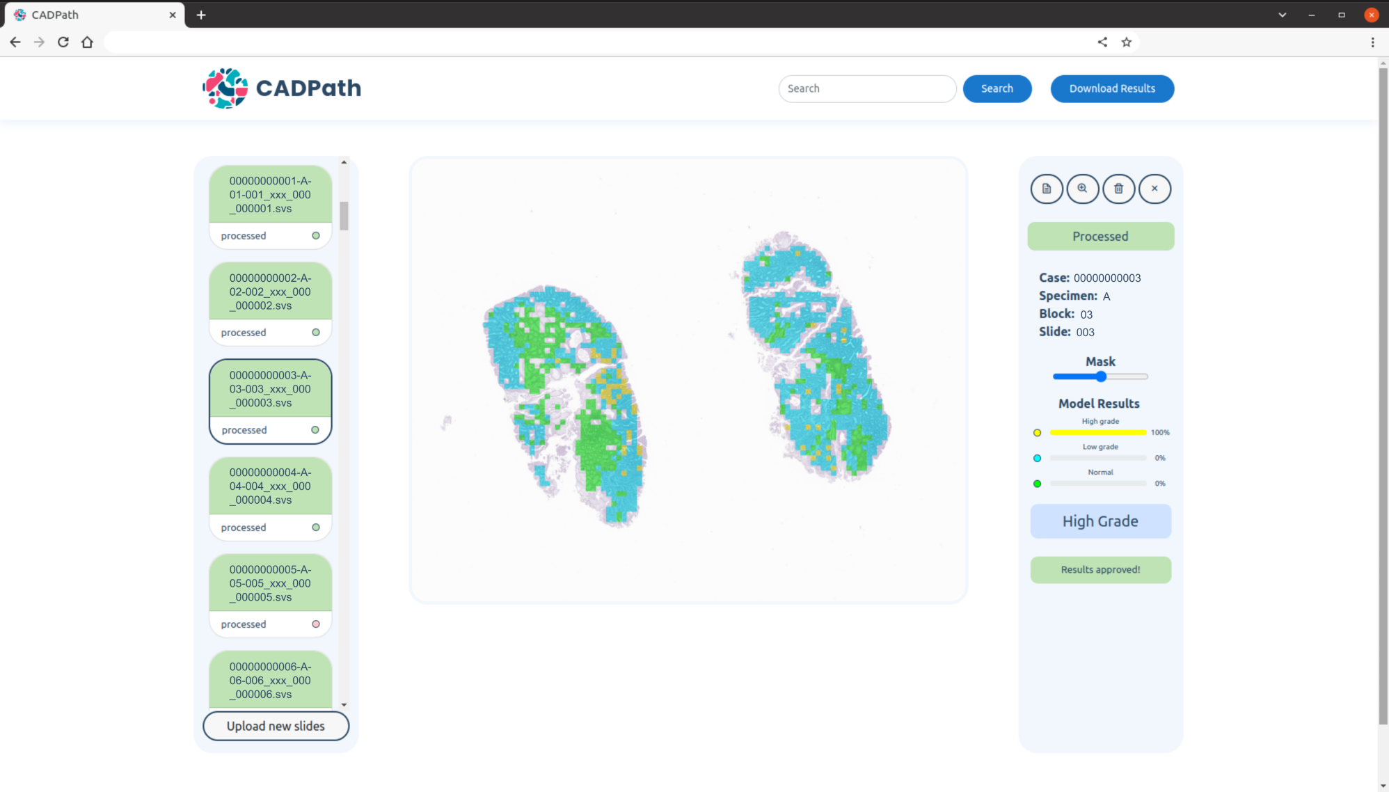
Figure 4: Main view of the CAD system prototype for CRS: Slide identification, confidence per class, diagnostic, mask overlay controller, results download as csv and slide search are some of the features visible. Slide identification is anonymised.

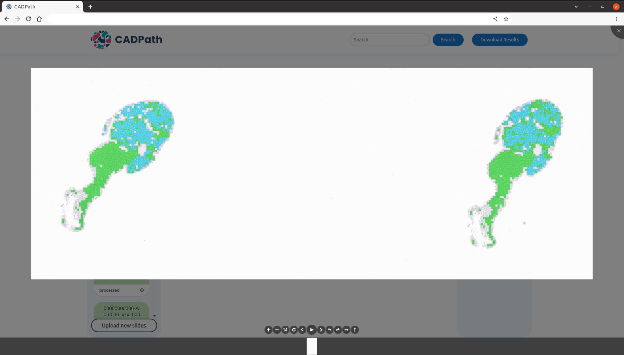
Figure 5: Zoomed view of a slide from the CAD system prototype, with the predictions map with a small overlay threshold. Slide identification is anonymised.

Furthermore, the prototype also allows user feedback where the user can accept/reject a result and provide a justification (Figure 6), an important feature for software updates, research development and possible active learning frameworks that can be developed in the future. These results can be downloaded with the corrected labels to allow for further retraining of the model.

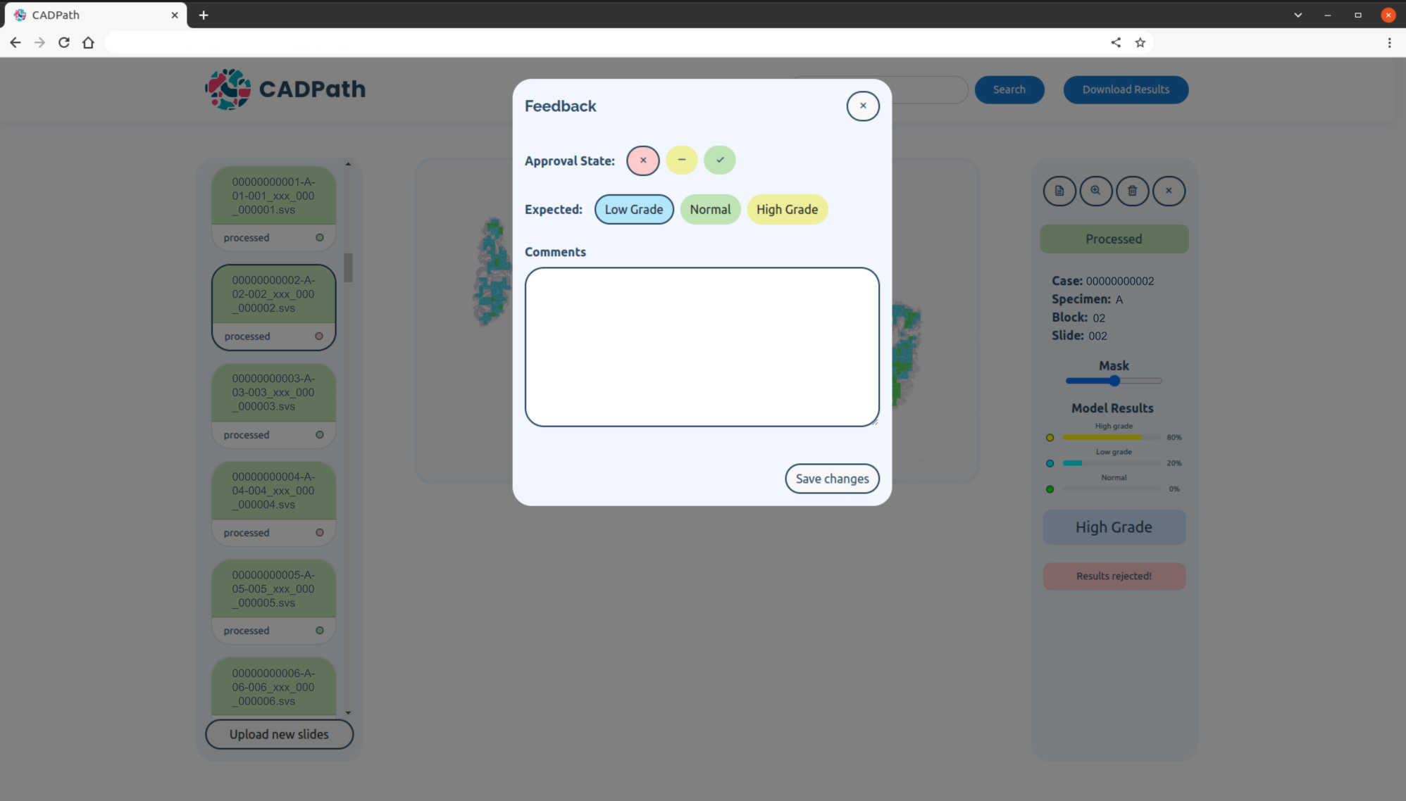
Figure 6: CAD system prototype report tool: the user can report if the result is either correct, wrong or inconclusive and leave a comment for each case individually. Slide identification is anonymised.

There are several advantages to developing such a system as a server-side web application. First, it does not require any specific installation or dedicated local storage in the user’s device. Secondly, it can be accessed at the same time by several pathologists from different locations, allowing for a quick review of a case by multiple pathologists without data transference. Moreover, the lack of local storage of clinical data increases the privacy of patient data, which can only be accessed through a highly encrypted virtual private network (VPN). Finally, all the processing can be moved to an efficient graphics processing unit (GPU), thus reducing the processing time by several orders of magnitude. Similar behaviour on a local machine would require the installation of dedicated GPUs in the pathologists’ personal devices. This platform is the first Pathology prototype for colorectal diagnosis developed in Portugal, and, as far as we know, one of the pioneers in the world. Its design was also carefully thought to be aligned with the needs of the pathologists.

3 Results

In this section, we present the results of the proposed method. The results are organised to first demonstrate the effectiveness of sampling, followed by an evaluation of the model in the two internal datasets (CRS10K and the prototype dataset), and finalise with the results on external datasets. We also discuss the advantages and disadvantages of the proposed approach, perform an analysis of the results from a clinical perspective, provide pathologists’ feedback on the use of the prototype, and finally discuss future directions.

3.1 On the effectiveness of sampling

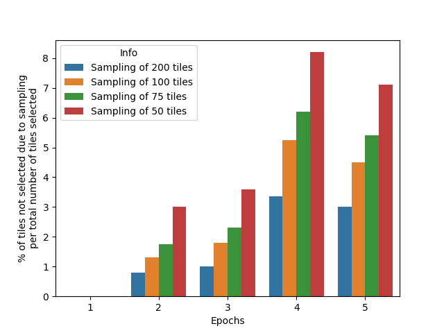
Figure 7: Tile sampling impact on information loss: percentage of tiles not selected due to sampling with different thresholds, over the first four inference epochs.

To find the most suitable threshold for sampling the tiles used in the weakly supervised training, we evaluated the percentage of relevant tiles that would be left out of the selection, if the original set was reduced to 75, 100, 150 or 200 tiles, over the first five inference epochs. A tile is considered relevant if it shares the same label as the slide, or if it would take part in the learning process in the weakly-supervised stage. As it is possible to see in Figure 7, if we set the maximum number of tiles to 200 after the second loop of inference, we would discard only 3.5% of the potentially informative tiles, in the worst-case scenario. On the other side of the spectrum, a more radical sampling of only 50 tiles would lead to a cut of up to 8%.

Moreover, to assess the impact of this sampling on the model’s performance, we also evaluated the accuracy and the QWK with and without sampling the top 200 tiles after the first inference iteration (Table 2). This evaluation considered sampling applied only to the training tile set, and to both the training and validation tile sets. As can be noticed, the performance is not degraded and the model is trained in a much faster way. In fact, using the setup previously mentioned, the first epoch of inference, with the full set of tiles takes 28h to be completed, while from the second loop the training time decreases to only 5h per epoch. Without sampling, training the model for 50 epochs would take around 50 days, whereas with sampling it takes around 10.

Table 2: Model performance comparison with and without tile sampling of the top 200 tiles from the first inference iteration. Compared the best epoch of the initial five epochs and of the initial ten epochs. Validation is represented as Val.

	Best Accuracy at		Best QWK at
Sampling	5th epoch	10th epoch	5th epoch	10th epoch
No	$84.94\%\pm 2.20$	$86.42\%\pm 2.11$	$0.809\pm 0.024$	$\textbf{0.829}\pm\textbf{0.023}$
Train	$85.43\%\pm 2.18$	$86.82\%\pm 2.08$	$0.817\pm 0.024$	$0.828\pm 0.023$
Train and Val.	$\textbf{86.12\%}\pm\textbf{2.13}$	$\textbf{86.92\%}\pm\textbf{2.08}$	$\textbf{0.824}\pm\textbf{0.023}$	$\textbf{0.829}\pm\textbf{0.023}$

3.2 CRS10K and Prototype

CRS10K test set and the prototype dataset were collected through different procedures. The first followed the same data collection process as the complete dataset, whereas the second originated from routine samples. Thus, the evaluation of both these sets is done separately.

Table 3: Model performance evaluation on the CRS10K test set. The binary accuracy is calculated as NNeo vs all. Accuracy is represented as (ACC). In bold are the best results per column.

Method	ACC	Binary ACC	Sensitivity
iMIL4Path	$91.33\%\pm 1.84$	$97.00\%\pm 1.11$	$\textbf{0.997}\pm\textbf{0.004}$
Ours (CRS4K)	$89.44\%\pm 2.01$	$96.11\%\pm 1.26$	$\textbf{0.997}\pm\textbf{0.004}$
Ours (CRS10K) wo/ Agg	$\textbf{93.44\%}\pm\textbf{1.62}$	$\textbf{97.78\%}\pm\textbf{0.96}$	$0.996\pm 0.005$
Ours (CRS10K) w/ Agg	$90.67\%\pm 1.90$	$97.55\%\pm 1.01$	$0.985\pm 0.009$

The first experiment was conducted on the CRS10K test set. As expected, the steep increase in the number of training samples led to a significantly better algorithm in this test set. Initially, the model trained on the CRS10K correctly predicted the class of 819 out of 900 samples. For the wrong 81 cases, the pathologists performed a blind review of these cases and found that the algorithm was indeed correct in 22 of them. This led to a correction in the labels of the test set, and the appropriate adjustment of the metrics. In Table 3, the performance of the different algorithms is presented. CRS10K outperforms the other approaches by a reasonable margin. We further applied the aggregation proposed by Neto et al. [31] to the best performing method, but without gains in performance. Despite being trained on the same dataset iMIL4Path and the proposed methodology trained on CRS4K, utilise different splits for training and validation, as well as different optimisation techniques due to the deterministic approach.

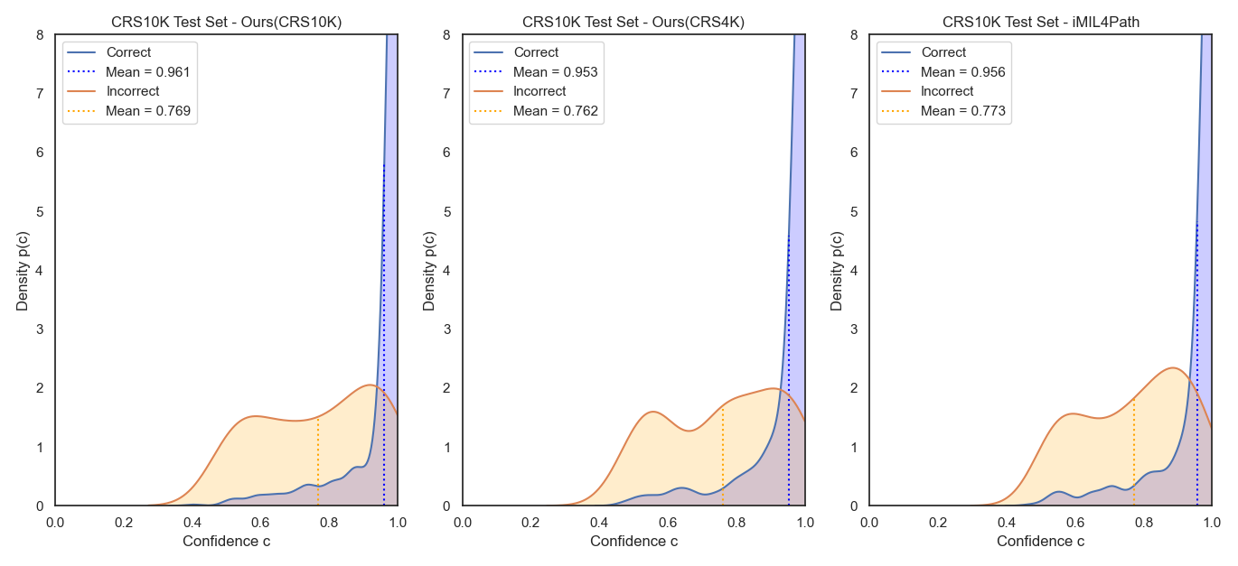
Figure 8: Kernel density estimation of the confidences of correct and incorrect predictions performed on the three-class classification problem by three distinct models on the CRS10K test set. The plots represent, from left to right, the proposed method trained on CRS10K, the proposed method trained on CRS4K and iMIL4Path.

In addition to examining quantitative metrics, such as the accuracy of the model, we extended our study to include an analysis of the confidence in the model when it correctly predicts a class and when it makes an incorrect prediction. To this end, we recorded the confidence of the model for the predicted class and divided it into the set of correct and incorrect predictions. These were then used to fit a kernel density estimator (KDE). Figure 8 shows the density estimation of the confidence values for the three different models. It is worth noting that, when correct, the model trained on the CRS10K, returns higher confidence levels as shown by the shift of its mean towards values close to one. On the other hand, the confidence values of its incorrect predictions decrease significantly, and although it does not present the lowest values, it shows the largest gap between correct and incorrect means.

Table 4: Model performance evaluation on the prototype test set. Accuracy is represented as (ACC). The binary accuracy is calculated as NNeo vs all. In bold are the best results per column.

Method	ACC	Binary ACC	Sensitivity
iMIL4Path	$\textbf{89.00}\%\pm\textbf{6.13}$	$96.00\%\pm 3.84$	$\textbf{1.000}\pm\textbf{0.000}$
Ours (CRS4K)	$85.00\%\pm 6.99$	$93.00\%\pm 5.00$	$\textbf{1.000}\pm\textbf{0.000}$
Ours (CRS10K) wo/ Agg	$\textbf{89.00}\%\pm\textbf{6.13}$	$\textbf{98.00}\%\pm\textbf{2.74}$	$0.986\pm 0.026$
Ours (CRS10K) w/ Agg	$85.00\%\pm 6.99$	$\textbf{98.00}\%\pm\textbf{2.74}$	$0.986\pm 0.026$

When tested on the prototype data (n=100), the importance of a higher volume of data remains visible (Table 4). Nonetheless, the performance of iMIL4Path [31] approach is comparable to the proposed approach trained on CRS10K. It is worth noting that the latter achieves better performance on the binary accuracy at the cost of a decrease in sensibility. In other words, the capability to detect negatives increases significantly. Due to the smaller set of slides, the confidence interval is much wider, as such, the performance on the CRS10K test set is a good indication of how these values would shift if more data was added. Similar performance drops were linked with the introduction of aggregation.

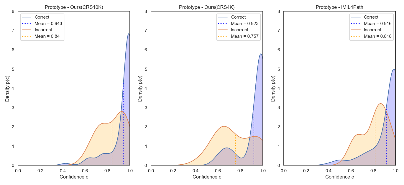
Figure 9: Kernel density estimation of the confidences of correct and incorrect predictions performed on the three-class classification problem by three distinct models on the prototype set. The plots represent, from left to right, the proposed method trained on CRS10K, the proposed method trained on CRS4K and iMIL4Path.

Despite similar results, the confidence of the model in its predictions is distinct in all three approaches, as seen in Figure 9. The proposed approach when trained on the CRS10K dataset has a larger density on values close to one when the predictions are correct, and the mean confidence of those predictions is, once more, higher than the other approaches. However, especially when compared to the proposed approach trained on the CRS4K, the confidence of wrong predictions is also higher. It can be a result of a larger set of wrong predictions available on the latter approach. Nonetheless, the steep increase in the density of values closer to one further indicates that there is room to explore other effects of extending the number of training samples, besides benefits in quantitative metrics.

3.3 Domain Generalisation Evaluation

To ensure the generalisation of the proposed approach across external datasets, we have evaluated their performance on TCGA and PAIP. Moreover, we conducted a similar analysis of both of these datasets, as the one done for the internal datasets.

Table 5: Model performance evaluation on the PAIP test set. The binary accuracy is calculated as NNeo vs all. Accuracy is represented as (ACC). In bold are the best results per column.

Method	ACC	Binary ACC	Sensitivity
iMIL4Path	$99.00\%\pm 1.95$	$\textbf{100.00\%}\pm\textbf{0.00}$	$\textbf{1.000}\pm\textbf{0.000}$
Ours (CRS4K)	$69.00\%\pm 9.06$	$\textbf{100.00\%}\pm\textbf{0.00}$	$\textbf{1.000}\pm\textbf{0.000}$
Ours (CRS10K) wo/ Agg	$\textbf{100.00\%}\pm\textbf{0.00}$	$\textbf{100.00\%}\pm\textbf{0.00}$	$\textbf{1.000}\pm\textbf{0.000}$
Ours (CRS10K) w/ Agg	$52.00\pm 9.79$	$\textbf{100.00\%}\pm\textbf{0.00}$	$\textbf{1.000}\pm\textbf{0.000}$

From the two datasets, PAIP is arguably the closest to CRS10K. It contains similar tissue, despite its colour differences. The performances of the proposed approaches were expected to match the performance of iMIL4Path in this dataset. However, it did not happen for the version trained on the CRS4K dataset, as seen in Table 5. A viable explanation concerns potential overfitting to the training data potentiated by an increase in the number of epochs of fully and weakly supervised training, a slight decrease in the tile variability in the latter approach, and a smaller number of samples when compared to the version trained on CRS10K. This version, trained on the larger set, mitigates the problems of the other method due to a significant increase in the training samples. Moreover, it is worth noting that in all three approaches, the errors corresponded only to a divergence between low and high-grade cases, with no non-neoplastic cases being classified as high-grade or vice-versa. As in previous sets, the version trained on the CRS10K dataset outperforms the remaining approaches. Using aggregation in this dataset leads to a discriminative power to distinguish between high- and low-grade lesions that is close to random.

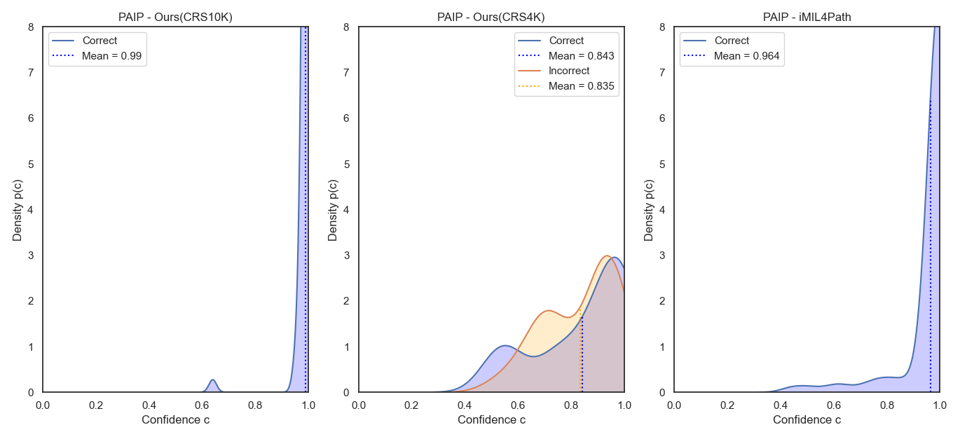
Figure 10: Kernel density estimation of the confidences of correct and incorrect predictions performed on the three-class classification problem by three distinct models on the PAIP dataset. The plots represent, from left to right, the proposed method trained on CRS10K, the proposed method trained on CRS4K and iMIL4Path.

In two of the three approaches, the number of incorrect samples is one or zero, as such, there is no density estimation for wrong samples in their confidence plot as seen in Figure 10. Yet, it is visible the shift towards higher values of confidence in the proposed approach trained on the CRS10K when compared to the method of iMIL4Path. The version trained on CRS4K shows very little separability between the confidence of correct and incorrect predictions.

Table 6: Model performance evaluation on the TCGA test set. The binary accuracy is calculated as NNeo vs all. Accuracy is represented as (ACC). In bold are the best results per column.

Method	ACC	Binary ACC	Sensitivity
iMIL4Path	$71.55\%\pm 5.80$	$80.60\%\pm 5.05$	$0.805\pm 0.051$
Ours (CRS4K) wo/ Agg	$70.69\%\pm 5.86$	$98.71\%\pm 1.45$	$0.991\pm 0.012$
Ours (CRS10K) wo/ Agg	$\textbf{84.91}\%\pm\textbf{4.61}$	$\textbf{99.13\%}\pm\textbf{1.19}$	$\textbf{0.996}\pm\textbf{0.008}$
Ours (CRS10K) w/ Agg	$69.83\%\pm 5.91$	$97.41\%\pm 2.04$	$0.983\pm 0.017$

The TCGA dataset has established itself as the most challenging for the proposed approaches. Besides the expected differences in colour and other elements, this dataset is mostly composed of resection samples, which are not present in the training dataset. As such, this presents itself as an excellent dataset to assess the capability of the model to handle these different types of samples. Both iMIL4Path and the proposed method trained on CRS4K have shown substantial problems in correctly classifying TCGA slides, as shown in Table 6. Despite having a lower performance on the general accuracy, the binary accuracy shows that our proposed method trained on CRS4K has much lower misclassification errors regarding the classification of high-grade samples as normal, demonstrating higher robustness of the new training approach against errors with a gap of two classes. As with other datasets, the proposed approach trained on CRS10K shows better results, this time by a significant margin with no overlapping between the confidence intervals.

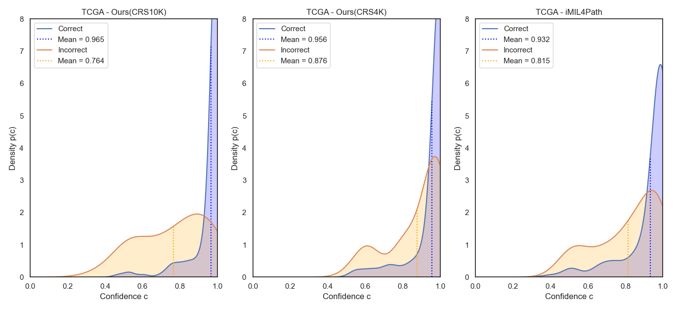
Figure 11: Kernel density estimation of the confidences of correct and incorrect predictions performed on the three-class classification problem by three distinct models on the TCGA dataset. The plots represent, from left to right, the proposed method trained on CRS10K, the proposed method trained on CRS4K and iMIL4Path.

Inspecting the predictions’ confidence for the three models indicates a behaviour in line with the accuracy-based performance (Figure 11). Moreover, a confidence shift of wrong predictions’ confidence towards smaller values is clearly visible in the plot corresponding to the model trained on CRS10K. The shown gap of 0.2 between the confidence of correct and wrong predictions, indicates that it is possible to quantify the uncertainty of the model and avoid the majority of the wrong predictions. In other words, when the uncertainty is above a learnt threshold, then the model refuses to make any prediction. It is extremely useful in models designed as a second opinion system.

3.4 Prototype usability in clinical practice

As it is currently designed, the algorithm works preferentially as a “second opinion”, allowing the assessment of difficult and troublesome cases, without the immediate need for the intervention of a second pathologist. Due to its “user-friendly” nature and very practical interface, the cases can be easily introduced into the system and results are rapidly shown and easily accessed. Also, by not only providing results but presenting visualisation maps (corresponding to each diagnostic class), the pathologist is able to compare his own remarks to those of the algorithm itself, towards a future “AI-assisted diagnosis”. Another relevant aspect is the fact that the prototype allows for user feedback (agreeing or not with the model’s proposed result), which can be further integrated into further updates of the software. Also interesting, is the possibility of using the prototype as a triage system on a pathologist’s daily workflow (by running front, before the pathologist checks the cases). Signalling the cases that would need to be more urgently observed (namely high-risk lesions) would allow the pathologists to prioritise their workflow. Further, by providing a previous assessment of the cases, it would also contribute to enhancing the pathologists’ efficiency. Although it is possible to use the model as it is upfront, it would classify some samples incorrectly (since it was not trained on the full spectrum of colorectal pathology). As such, the uncertainty quantification based on the provided confidence given in the user interface could also be extremely useful. Presently, there is no recommendation for dual independent diagnosis of colorectal biopsies (contrary to gastric biopsies, where, in cases in which surgical treatment is considered, it is recommended to obtain a pre-treatment diagnostic second opinion  [42]), but, in case that in the future this also becomes a requirement, a tool such as CADPath.AI prototype could assist in this task. This has increased importance due to the worldwide shortage of pathologists and so, such CAD tools can really make a difference in patient care (in similarity, for example, with Google Health’s research, using deep learning to screen diabetic retinopathy in low/middle-income countries, in which the system showed real-time retinopathy detection capability similar to retina specialists, alleviating the significant manpower constrictions in this setting  [43]). Lastly, we also anticipate that this prototype, and similar tools, can be used in a teaching environment since its easy use and explainable capability (through the visualisation maps) allows for easy understanding of the given classifications and having a web-based interface allows for easy sharing.

3.5 Future work

The proposed algorithm still has potential for improvement. We aim to include the recognition of serrated lesions, to distinguish normal mucosa from significant inflammatory alterations/diseases, to stratify high-risk lesions into high-grade dysplasia and invasive carcinomas and to identify other neoplasia subtypes. Further, we would like to leverage the model to be able to evaluate also surgical specimens. Another relevant step will be the merge of our dataset and external ones for training, besides only testing it on external samples. This will enhance its generalisation capabilities and provide a more robust system. Lastly, we intend to measure the “user experience” and feedback from the pathologists, by its gradual implementation in general laboratory routine work.

The following goals comprise a more extensive evaluation of the model across more scanner brands and labs. We also want to promote certain behaviours that would allow for more direct and integrated uncertainty estimation. We have also been looking towards aggregation methods, but, since in the majority of them there is an increased risk of false negatives, we have work to do in that research direction.

4 Discussion

In this document, we have redesigned the previous methodology on MIL for colorectal cancer diagnosis. First, we extended and leveraged the mixed supervision approach to design a sampling strategy, which utilises the knowledge from the full supervision training as a proxy to tile utility. Secondly, we studied the confidence that the model shows in its predictions when they are correct and when they are incorrect. Additionally, this confidence is shown to be a potential resource to quantify uncertainty and avoid wrong predictions on low-certainty scenarios. This is entirely integrated within a web-based prototype to aid pathologists in their routine work.

The proposed methodology was evaluated on several datasets, including two external sets. Through this evaluation, it was possible to infer that the performance of the proposed methodology benefits from a larger dataset and surpasses the performance of previous state-of-the-art models. As such, and given the excelling results that originated from the increase in the dataset, we are also publicly releasing the majority of the CRS10K dataset, one of the largest publicly available colorectal datasets composed of H&E images in the literature, including the test set for the benchmark of distinct approaches across the literature.

Finally, we have clearly defined a set of potential future directions to be explored, either for better model design, the development of useful prototypes or even the integration of uncertainty in the predictions.

References

- [1] International Agency for Research on Cancer (IARC), Global cancer observatory, https://gco.iarc.fr/ (2022).
- [2] H. Brody, Colorectal cancer, Nature 521 (2015) S1. doi:10.1038/521S1a.
- [3] D. Holmes, A disease of growth, Nature 521 (2015) S2–S3. doi:10.1038/521S2a.
- [4] Digestive Cancers Europe (DiCE), Colorectal screening in europe, https://bit.ly/3rFxSEL.
- [5] C. Hassan, G. Antonelli, J.-M. Dumonceau, J. Regula, M. Bretthauer, S. Chaussade, E. Dekker, M. Ferlitsch, A. Gimeno-Garcia, R. Jover, M. Kalager, M. Pellisé, C. Pox, L. Ricciardiello, M. Rutter, L. M. Helsingen, A. Bleijenberg, C. Senore, J. E. van Hooft, M. Dinis-Ribeiro, E. Quintero, Post-polypectomy colonoscopy surveillance: European society of gastrointestinal endoscopy guideline - update 2020, Endoscopy 52 (8) (2020) 687–700. doi:10.1055/a-1185-3109.
- [6] D. Mahajan, E. Downs-Kelly, X. Liu, R. Pai, D. Patil, L. Rybicki, A. Bennett, T. Plesec, O. Cummings, D. Rex, J. Goldblum, Reproducibility of the villous component and high-grade dysplasia in colorectal adenomas 1 cm: Implications for endoscopic surveillance, American Journal of Surgical Pathology 37 (3) (2013) 427–433. doi:10.1097/PAS.0b013e31826cf50f.
- [7] S. Gupta, D. Lieberman, J. C. Anderson, C. A. Burke, J. A. Dominitz, T. Kaltenbach, D. J. Robertson, A. Shaukat, S. Syngal, D. K. Rex, Recommendations for follow-up after colonoscopy and polypectomy: A consensus update by the us multi-society task force on colorectal cancer, Gastrointestinal Endoscopy (2020). doi:10.1016/j.gie.2020.01.014.
-
[8]
C. Eloy, J. Vale, M. Curado, A. Polónia, S. Campelos, A. Caramelo, R. Sousa,
M. Sobrinho-Simões, Digital
pathology workflow implementation at ipatimup, Diagnostics 11 (11) (2021).
doi:10.3390/diagnostics11112111.
URL https://www.mdpi.com/2075-4418/11/11/2111 -
[9]
F. Fraggetta, A. Caputo, R. Guglielmino, M. G. Pellegrino, G. Runza,
V. L’Imperio, A survival
guide for the rapid transition to a fully digital workflow: The
“caltagirone example”, Diagnostics 11 (10) (2021).
doi:10.3390/diagnostics11101916.
URL https://www.mdpi.com/2075-4418/11/10/1916 - [10] D. Montezuma, A. Monteiro, J. Fraga, L. Ribeiro, S. Gonçalves, A. Tavares, J. Monteiro, I. Macedo-Pinto, Digital pathology implementation in private practice: Specific challenges and opportunities, Diagnostics 12 (2) (2022) 529.
- [11] A. Madabhushi, G. Lee, Image analysis and machine learning in digital pathology: challenges and opportunities, Medical Image Analysis 33 (2016) 170–175. doi:10.1016/j.media.2016.06.037.
- [12] E. A. Rakha, M. Toss, S. Shiino, P. Gamble, R. Jaroensri, C. H. Mermel, P.-H. C. Chen, Current and future applications of artificial intelligence in pathology: a clinical perspective, Journal of Clinical Pathology (2020). doi:10.1136/jclinpath-2020-206908.
- [13] M. Veta, P. J. van Diest, S. M. Willems, H. Wang, A. Madabhushi, A. Cruz-Roa, F. Gonzalez, A. B. Larsen, J. S. Vestergaard, A. B. Dahl, D. C. Cireşan, J. Schmidhuber, A. Giusti, L. M. Gambardella, F. B. Tek, T. Walter, C.-W. Wang, S. Kondo, B. J. Matuszewski, F. Precioso, V. Snell, J. Kittler, T. E. de Campos, A. M. Khan, N. M. Rajpoot, E. Arkoumani, M. M. Lacle, M. A. Viergever, J. P. Pluim, Assessment of algorithms for mitosis detection in breast cancer histopathology images, Medical Image Analysis 20 (1) (2015) 237–248. doi:10.1016/j.media.2014.11.010.
- [14] G. Campanella, M. G. Hanna, L. Geneslaw, A. Miraflor, V. Werneck Krauss Silva, K. J. Busam, E. Brogi, V. E. Reuter, D. S. Klimstra, T. J. Fuchs, Clinical-grade computational pathology using weakly supervised deep learning on whole slide images, Nat. Med. 25 (8) (2019) 1301–1309. doi:10.1038/s41591-019-0508-1.
- [15] S. P. Oliveira, J. Ribeiro Pinto, T. Gonçalves, R. Canas-Marques, M.-J. Cardoso, H. P. Oliveira, J. S. Cardoso, Weakly-supervised classification of HER2 expression in breast cancer haematoxylin and eosin stained slides, Applied Sciences 10 (14) (2020) 4728. doi:10.3390/app10144728.
- [16] T. Albuquerque, A. Moreira, J. S. Cardoso, Deep ordinal focus assessment for whole slide images, in: Proceedings of the IEEE/CVF International Conference on Computer Vision, 2021, pp. 657–663.
- [17] S. P. Oliveira, P. C. Neto, J. Fraga, D. Montezuma, A. Monteiro, J. Monteiro, L. Ribeiro, S. Gonçalves, I. M. Pinto, J. S. Cardoso, CAD systems for colorectal cancer from WSI are still not ready for clinical acceptance, Scientific Reports 11 (1) (2021) 14358. doi:10.1038/s41598-021-93746-z.
- [18] N. Thakur, H. Yoon, Y. Chong, Current trends of artificial intelligence for colorectal cancer pathology image analysis: a systematic review, Cancers 12 (7) (2020). doi:10.3390/cancers12071884.
- [19] Y. Wang, X. He, H. Nie, J. Zhou, P. Cao, C. Ou, Application of artificial intelligence to the diagnosis and therapy of colorectal cancer, Am. J. Cancer Res. 10 (11) (2020) 3575–3598.
- [20] A. Davri, E. Birbas, T. Kanavos, G. Ntritsos, N. Giannakeas, A. T. Tzallas, A. Batistatou, Deep learning on histopathological images for colorectal cancer diagnosis: A systematic review, Diagnostics 12 (4) (2022) 837.
- [21] O. Iizuka, F. Kanavati, K. Kato, M. Rambeau, K. Arihiro, M. Tsuneki, Deep learning models for histopathological classification of gastric and colonic epithelial tumours, Scientific Rep. 10 (2020). doi:10.1038/s41598-020-58467-9.
- [22] H. Tizhoosh, L. Pantanowitz, Artificial intelligence and digital pathology: challenges and opportunities, J. Pathol. Inform 9 (1) (2018). doi:10.4103/jpi.jpi\_53\_18.
- [23] J. W. Wei, A. A. Suriawinata, L. J. Vaickus, B. Ren, X. Liu, M. Lisovsky, N. Tomita, B. Abdollahi, A. S. Kim, D. C. Snover, J. A. Baron, E. L. Barry, S. Hassanpour, Evaluation of a deep neural network for automated classification of colorectal polyps on histopathologic slides, JAMA Network Open 3 (4) (2020). doi:10.1001/jamanetworkopen.2020.3398.
- [24] Z. Song, C. Yu, S. Zou, W. Wang, Y. Huang, X. Ding, J. Liu, L. Shao, J. Yuan, X. Gou, W. Jin, Z. Wang, X. Chen, H. Chen, C. Liu, G. Xu, Z. Sun, C. Ku, Y. Zhang, X. Dong, S. Wang, W. Xu, N. Lv, H. Shi, Automatic deep learning-based colorectal adenoma detection system and its similarities with pathologists, BMJ Open 10 (9) (2020). doi:10.1136/bmjopen-2019-036423.
- [25] L. Xu, B. Walker, P.-I. Liang, Y. Tong, C. Xu, Y. Su, A. Karsan, Colorectal cancer detection based on deep learning, J. Pathol. Inf. 11 (1) (2020). doi:10.4103/jpi.jpi\_68\_19.
- [26] K.-S. Wang, G. Yu, C. Xu, X.-H. Meng, J. Zhou, C. Zheng, Z. Deng, L. Shang, R. Liu, S. Su, et al., Accurate diagnosis of colorectal cancer based on histopathology images using artificial intelligence, BMC medicine 19 (1) (2021) 1–12. doi:10.1186/s12916-021-01942-5.
- [27] G. Yu, K. Sun, C. Xu, X.-H. Shi, C. Wu, T. Xie, R.-Q. Meng, X.-H. Meng, K.-S. Wang, H.-M. Xiao, et al., Accurate recognition of colorectal cancer with semi-supervised deep learning on pathological images, Nature communications 12 (1) (2021) 1–13.
- [28] N. Marini, S. Otálora, F. Ciompi, G. Silvello, S. Marchesin, S. Vatrano, G. Buttafuoco, M. Atzori, H. Müller, Multi-scale task multiple instance learning for the classification of digital pathology images with global annotations, in: M. Atzori, N. Burlutskiy, F. Ciompi, Z. Li, F. Minhas, H. Müller, T. Peng, N. Rajpoot, B. Torben-Nielsen, J. van der Laak, M. Veta, Y. Yuan, I. Zlobec (Eds.), Proceedings of the MICCAI Workshop on Computational Pathology, Vol. 156 of Proceedings of Machine Learning Research, PMLR, 2021, pp. 170–181.
- [29] C. Ho, Z. Zhao, X. F. Chen, J. Sauer, S. A. Saraf, R. Jialdasani, K. Taghipour, A. Sathe, L.-Y. Khor, K.-H. Lim, et al., A promising deep learning-assistive algorithm for histopathological screening of colorectal cancer, Scientific Reports 12 (1) (2022) 1–9.
- [30] T. Albuquerque, A. Moreira, B. Barros, D. Montezuma, S. P. Oliveira, P. C. Neto, J. Monteiro, L. Ribeiro, S. Gonçalves, A. Monteiro, I. M. Pinto, J. S. Cardoso, Quality control in digital pathology: Automatic fragment detection and counting, in: 2022 44th Annual International Conference of the IEEE Engineering in Medicine & Biology Society (EMBC), 2022, pp. 588–593. doi:10.1109/EMBC48229.2022.9871208.
- [31] P. C. Neto, S. P. Oliveira, D. Montezuma, J. Fraga, A. Monteiro, L. Ribeiro, S. Gonçalves, I. M. Pinto, J. S. Cardoso, imil4path: A semi-supervised interpretable approach for colorectal whole-slide images, Cancers 14 (10) (2022) 2489.
- [32] Pathcore, Sedeen viewer, https://pathcore.com/sedeen (2020).
- [33] P. A. Platform, Paip, http://www.wisepaip.org, last accessed on 20/01/22 (2020).
- [34] K. Clark, B. Vendt, K. Smith, J. Freymann, J. Kirby, P. Koppel, S. Moore, S. Phillips, D. Maffitt, M. Pringle, L. Tarbox, F. Prior, The cancer imaging archive (TCIA): Maintaining and operating a public information repository, Journal of Digital Imaging 26 (2013) 1045–1057. doi:10.1007/s10278-013-9622-7.
- [35] S. Kirk, Y. Lee, C. A. Sadow, S. Levine, C. Roche, E. Bonaccio, J. Filiippini, Radiology data from the cancer genome atlas colon adenocarcinoma [TCGA-COAD] collection. (2016). doi:10.7937/K9/TCIA.2016.HJJHBOXZ.
- [36] S. Kirk, Y. Lee, C. A. Sadow, S. Levine, Radiology data from the cancer genome atlas rectum adenocarcinoma [TCGA-READ] collection. (2016). doi:10.7937/K9/TCIA.2016.F7PPNPNU.
- [37] N. Otsu, A threshold selection method from gray-level histograms, IEEE Transactions on Systems, Man, and Cybernetics 9 (1) (1979) 62–66. doi:10.1109/TSMC.1979.4310076.
- [38] J. Božič, D. Tabernik, D. Skočaj, Mixed supervision for surface-defect detection: From weakly to fully supervised learning, Computers in Industry 129 (2021) 103459.
- [39] S. Raschka, Model evaluation, model selection, and algorithm selection in machine learning, arXiv preprint arXiv:1811.12808 (2018).
- [40] K. He, X. Zhang, S. Ren, J. Sun, Deep residual learning for image recognition, in: Proceedings of the IEEE conference on computer vision and pattern recognition, 2016, pp. 770–778. doi:10.1109/CVPR.2016.90.
- [41] D. P. Kingma, J. Ba, Adam: A method for stochastic optimization, in: ICLR (Poster), 2015.
- [42] W. C. of Tumours Editorial Board, WHO classification of tumours of the digestive system, no. Ed. 5, World Health Organization, 2019.
- [43] P. Ruamviboonsuk, R. Tiwari, R. Sayres, V. Nganthavee, K. Hemarat, A. Kongprayoon, R. Raman, B. Levinstein, Y. Liu, M. Schaekermann, et al., Real-time diabetic retinopathy screening by deep learning in a multisite national screening programme: a prospective interventional cohort study, The Lancet Digital Health 4 (4) (2022) e235–e244.