A Comprehensive Review on Autonomous Navigation

Abstract.

The field of autonomous mobile robots has undergone dramatic advancements over the past decades. Despite achieving important milestones, several challenges are yet to be addressed. Aggregating the achievements of the robotic community as survey papers is vital to keep the track of current state-of-the-art and the challenges that must be tackled in the future. This paper tries to provide a comprehensive review of autonomous mobile robots covering topics such as sensor types, mobile robot platforms, simulation tools, path planning and following, sensor fusion methods, obstacle avoidance, and SLAM. The urge to present a survey paper is twofold. First, autonomous navigation field evolves fast so writing survey papers regularly is crucial to keep the research community well-aware of the current status of this field. Second, deep learning methods have revolutionized many fields including autonomous navigation. Therefore, it is necessary to give an appropriate treatment of the role of deep learning in autonomous navigation as well which is covered in this paper. Future works and research gaps will also be discussed.

1. Introduction

Robotics have impacted our lives in many ways. Backed up by technological advancements, robots have found their way in several application domains such as medical (Di Lallo et al., 2021; Barducci et al., 2019; Li et al., 2018; Sitti, 2018), military (Patil et al., 2020; Ha et al., 2019; Yamauchi, 2004), industrial (Huynh et al., 2020; Bader and Rahimifard, 2020; kuk, [n. d.]b; Levine et al., 2015; Yu et al., 2021), space (Nesnas et al., 2021; Maurette, 2003; Volpe et al., 1996; Maimone et al., 2006; Bajracharya et al., 2008), agricultural (Libin et al., 2008; Monta et al., 1995; Foglia and Reina, 2006; Edan, 1995; Zhang et al., 2020; Malavazi et al., 2018), etc. Adding autonomous navigation ability to robot platforms boosts their performance significantly since they can reach wherever they are needed on their own. This motivation has driven researchers to push the autonomous navigation technology to its limits. Given the rich and fast-evolving literature on the topic of autonomous navigation, it is necessary to prepare literature surveys on regular basis. This way, experienced researchers, as well as newcomers, can get an insight into the current state-of-the-art in autonomous navigation which is the inspiration for this survey.

The journey toward autonomous mobile robots has been started with development of first-ever general-purpose mobile robot named Shakey (Nilsson et al., 1984). Developed by Artificial Intelligence Center of Stanford Research Institute, Shakey had the ability to reason about its own actions. Another notable mobile robot is CART (Adams, 1961; Earnest, 2012) which was capable of line following using a camera and a radio control link. The required processing was done on a mainframe computer which was connected to CART via the aforementioned radio link. There have also been attempts at the development of mobile robots for space missions. For example, Lunokhod (Kassel, 1971; Lun, [n. d.]) was developed by Soviet Union for moon exploration or the United States developed Viking Mars landers (VL-1, and VL-2) for measurement of atmospheric temperature, wind speed and direction, and pressure (Hess et al., 1977) as well as Mars rover Sojourner (Mishkin et al., 1998).

Autonomous navigation has made constant progress over the years. Autonomous mobile robots were developed to drive (Dic, [n. d.]; Keirsey et al., 1987; Dickmanns, 2007; Oagana, 2013; Pomerleau, 1994), operate as medical assistance in hospitals (Nocks, 2007), explore active volcanoes (Dante I and II) (Krotkov et al., 1994; Bares and Wettergreen, 1999), etc. The progress has even been boosted by holding international competitions focused on autonomous mobile robots. The DARPA grand challenge held in 2004 (dar, [n. d.]a) was a turning point in the field of autonomous mobile robots. In this competition, autonomous cars were tasked to navigate a 240km off-road path without human intervention. Although none of the contenders managed to reach the finish line, valuable lessons were learned from the experienced failures. The challenge was repeated a year later and this time, five of the autonomous vehicles reached the finish line; among them, Stanley (Thrun et al., 2006) from Stanford University claimed first place. In 2006, yet another grand challenge was held but this time in urban environments (dar, [n. d.]b). The objective was to navigate through an urban area while complying with traffic regulations and avoiding collisions with obstacles. The winner of this contest was vehicle Boss of team Tartan (Urmson et al., 2007) developed in a collaborative effort by Carnegie Mellon University and General Motors.

Researchers have also worked on multi-robot setups. Swarm-bots project (Groß et al., 2006) was focused on self-organizing swarm of simple robots to achieve complex tasks. Swarm of autonomous underwater vehicles for performing stealthy underwater missions has also been investigated yielding a method called Suave (Swarm Underwater Autonomous Vehicle localization) (Liu et al., 2014). This method reduces the frequency of going to water surface for obtaining position information from external sources such as satellites. This way, the probability of being compromised for the stealthy underwater mission is reduced. In 2010, there has also been an international contest called MAGIC (Multi Autonomous Ground-Robotic International Challenge) (Aplin et al., 2010) devoted to group of autonomous robots working together.

Obviously, multiple survey papers have already been published on the subject of autonomous mobile robots. To highlight the differences between our survey and existing ones, table 1 has been prepared in which existing surveys have been sorted according to their publication year. As can be seen in table 1, some of the topics are missing in previous surveys but are covered in this paper. For example, Niloy et al. (Niloy et al., 2021) have only focused on indoor autonomous navigation. The survey by Pol and Murugan (Pol and Murugan, 2015) is also limited to indoor navigation except that human presence in the environment has been considered.

Mohanty and Parhi (Mohanty and Parhi, 2013) have primarily focused on requirements of global and local path planning and navigation. In Guzel’s survey (Güzel, 2013), the primary topic is mapless, vision-based navigation but some map-based methods have been reviewed as well. However, SLAM and several other important topics are absent. Injarapu and Gawre (Injarapu and Gawre, 2017) have only considered path planning and legacy methods for obstacle avoidance. Pandey et al. (Pandey et al., 2017) have divided mobile robot navigation algorithms into three groups deterministic, non-deterministic, and evolutionary algorithms. Similar to some other surveys, Pandey et al. divide navigation into global and local (Ni et al., 2016). Again, some topics such as SLAM and modern obstacle avoidance methods are missing from (Pandey et al., 2017). Victerpaul et al. (Victerpaul et al., 2017) have special emphasis on path planning approaches and have also covered related topics such as navigation and legacy obstacle avoidance. Tzafestas (Tzafestas, 2018) has covered most of the topics but lacks the review of modern obstacle avoidance methods, simulation tools, etc. Alatise and Hancke (Alatise and Hancke, 2020) have covered multiple topics such as sensor types, autonomous mobile robots challenges, classical obstacle avoidance methods, sensor fusion, etc.; however, other important topics such as SLAM and newer obstacle avoidance methods based on reinforcement learning (RL) or deep learning (DL) have not been covered.

Ibanez et al. (Sánchez-Ibáñez et al., 2021) have reviewed path planning methods with special focus on path planners for ground vehicles which can be extended to other platforms such as autonomous boats. However, SLAM, modern obstacle avoidance, sensor fusion, etc. are missing from (Sánchez-Ibáñez et al., 2021). Panigrahi and Bisoy (Panigrahi and Bisoy, 2021) have not investigated path following/planning, simulation tools, etc. Zghair and Al-Araji (Zghair and Al-Araji, 2021) have investigated the evolution of control systems of mobile robots for the past decade. Again, modern obstacle avoidance methods and simulation tools are missing from their survey.

Table 1. Comparison between our survey and previous ones.

Year

2013

2013

2015

2017

2017

2017

2018

2020

2021

2021

2021

2021

-

Reference

(Mohanty and Parhi, 2013)

(Güzel, 2013)

(Pol and Murugan, 2015)

(Injarapu and Gawre, 2017)

(Pandey et al., 2017)

(Victerpaul et al., 2017)

(Tzafestas, 2018)

(Alatise and Hancke, 2020)

(Sánchez-Ibáñez et al., 2021)

(Panigrahi and Bisoy, 2021)

(Niloy et al., 2021)

(Zghair and Al-Araji, 2021)

ours

Covered topics

Sensor types

✓

✓

✓

✓

Mobile robot platform types

✓

✓

✓

✓

Simulation tools

✓

Path planning

✓

✓

✓

✓

✓

✓

✓

✓

✓

✓

✓

Path following

✓

✓

✓

✓

✓

Sensor fusion

✓

✓

✓

✓

✓

✓

Obstacle avoidance

Legacy

✓

✓

✓

✓

✓

✓

✓

✓

✓

✓

✓

✓

RL/DL

✓

✓

✓

Navigation

Map-based

✓

✓

✓

✓

✓

✓

✓

✓

✓

✓

✓

✓

Mapless

✓

✓

✓

✓

✓

✓

✓

✓

✓

✓

✓

✓

SLAM

✓

✓

✓

✓

✓

Based on the shortcomings of the previous surveys mentioned above, this survey has been prepared to cover all the topics listed in table 1. We have striven to:

• give a comprehensive treatment on legacy as well as modern obstacle avoidance methods (based on RL and DL)

• review the most notable SLAM methods

• introduce well-known robotic simulators and whether they can be linked to robotic operating system (ROS) or not (ros, [n. d.])

• types of mobile robot platforms and their characteristics based on their operational environment

• Simple and concise review of famous sensor fusion approaches such as Kalman filter (Kalman, 1960) and its extensions as well as particle filter (Gordon et al., 1993)

• review open source SLAM datasets

The rest of this survey is structured as follows. Section 2 is devoted to different types of sensors used for autonomous navigation. Section 3 reviews different types of mobile robot platforms and their characteristics. Common software for robotic simulations is reviewed in section 4. Path planning and path following approaches are reviewed in sections 5 and 6, respectively. Sensor fusion methods are reviewed in section 7. Obstacle avoidance is investigated in section 8. Navigation and SLAM methods are reviewed in sections 9 and 10, respectively. The survey is closed with future works and conclusion in sections 11 and 12, respectively.

2. Sensors

Acting autonomously is not possible without the ability to sense the surrounding environment (Russell and Norvig, 2009). Any autonomous robot must be equipped with a perception module which is combination of hardware (sensors) and software components. This section is devoted to various types of sensors that are commonly used in autonomous mobile robots.

2.1. Absolution positioning sensors

Mobile robots need to move in their operational environment in order to carry out their objectives at different positions in the environment. For example, a rescue robot needs to navigate toward the wounded victim in order to perform the rescue operation. An important prerequisite to autonomous navigation is the self-localization ability of the robot. Usually, localization is performed with respect to some reference frame in the environment.

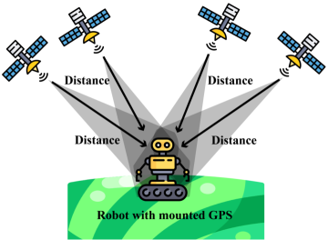
Global positioning system (GPS) receiver is one of the common sensors that provides absolute positioning in terms of longitude and latitude as well as time data anywhere on or near the Earth based on information received from low Earth orbiting satellites. The receiver uses the difference between the reception time of satellite signal and its broadcast time to compute its distance from the satellite. As shown in figure 1a, having access to information from at least four satellites, the receiver can provide positioning information accurate to a few meters for outdoor navigation. The drawback of GPS is that localization data becomes unreliable if unobstructed line of sight to at least four satellites is unavailable. In urban areas, signal outages may be caused by tall buildings or mountains (gps, [n. d.]). Additionally GPS signals are not available inside indoor environments.

(a)

(b)

Figure 1. Illustration of (a) robot localization using GPS receiver and (b) DGPS localization and error correction using reference station.

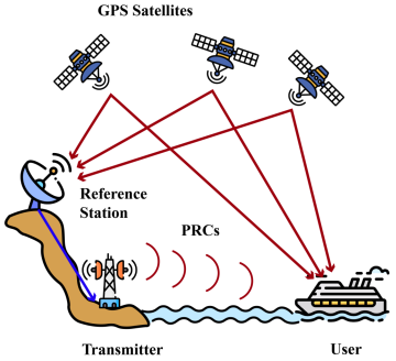
The localization error of GPS can be reduced by using differential GPS (DGPS). Basically, DGPS relies on multiple fixed beacons with known locations on the Earth. These beacons compare their known positions with the ones computed based on received satellite signals and broadcast correction information as shown in figure 1b. GPS receivers can reduce their positioning error using corrective signals broadcast by these beacons. The drawback of DGPS is that the quality of correction degrades as we move away from base/reference station (Barr et al., 2013).

2.2. Obstacle detection sensors

In this section, different types of sensors that are commonly used for obstacle detection and avoidance are introduced.

(a)

(b)

(c)

Figure 2. Different types of cameras: (a) mono, (b) stereo/RGBD, and (c) Stabilized vision system

2.2.1. Visual sensors

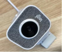
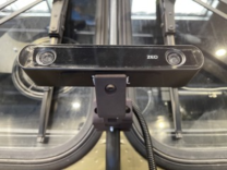
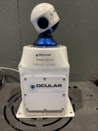
Claiming that a robotic system has autonomous navigation capability is almost impossible without equipping the robot with means of obstacle detection and avoidance. One can think of variety of sensor types when it comes to obstacle detection. Monocular (figure 2a) and stereo/RGBD cameras (figure 2b) provide feature-rich visual data at a reasonable price. The emergence of powerful vision algorithms based on DL and relatively affordable edge devices with reasonable processing power such as Jetson boards (jet, [n. d.]) has made visual sensors an ideal choice for performing various vision tasks including obstacle detection. During the robot movement, the onboard cameras may be subject to vibration making captured images blurry. This issue is addressed by stabilized vision systems (Rob, [n. d.]) an example of which is shown in figure 2c. Stabilized vision systems also improve the tracking capability.

2.2.2. Range sensors

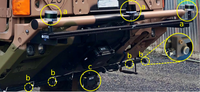
One of the most convenient solutions for obstacle detection is using range sensors which measure time-of-flight. Radar (Radio Detection And Ranging) relies on radio waves to detect distance and angle to objects and/or their velocity. A typical Radar has been depicted in figure 3. LiDAR (light detection and ranging) does similar thing to Radar but instead of using radio waves, it uses pulsed laser light. LiDAR sensors are capable of measuring range data with higher accuracy compared to Radar. The downside of these sensors is their high price. Moreover, laser scanners cannot sense glass obstacles and they cannot be used underwater due to laser disruption by water (Riisgaard and Blas, 2003). Typical LiDARs have been shown in figure 3.

Ultrasonic sensors also provide range data but with much less precision compared to LiDAR and RADAR. The total range of ultrasonic sensor is lower (about seven meters) than LiDAR and RADAR. The lower precision of ultrasonic sensor is due to the fact that its radiation pattern is bat-like. Therefore, after receiving the reflection of an emitted signal that hits an obstacle, the position of the sensed obstacle can only be estimated vaguely within the region covered by the emitted wave. This is in contrast to LiDAR and RADAR that provide much more accurate data about the obstacle position. A typical ultrasonic sensor has been shown in figure 3.

Figure 3. Different types of range sensors: (a) LiDAR, (b) Ultrasonic, (c) RADAR.

2.3. Relative positioning sensors

In section 2.1, absolute positioning sensors were reviewed. However, there are scenarios that absolution positioning is not possible which is the motivation for using relative positioning sensors such as inertial measurement unit (IMU) and encoder. IMU is composed of three accelerometers and three gyroscopes along $\{x,y,z\}$ axes. When IMU is mounted on the robot, the accelerometers and gyroscopes measure the robot acceleration and rotation rate along the three axes, respectively. Using the well-established mathematics of an inertial navigation system (INS) (Titterton et al., 2004), it is possible to turn IMU readings into useful 3D position and 3D orientation for the robot. Due to successive integration of IMU data, the estimated robot pose is subject to accumulated error which can be reduced by fusing INS data with other sensors such as GPS and camera(s) (see section 7.4).

Another sensor that can be used for relative positioning in ground robots is rotary encoder. Mounting encoder on a robot wheel, it is possible to count the number of rounds the wheel has completed. Knowing the perimeter of the wheel, the amount of robot displacement can be estimated. The drawback of using encoders is that wheel slippage leads to erroneous displacement estimates.

3. Mobile robot platforms

Over the years, different types of mobile robot platforms have been designed and developed. Mobile robots may be ground (Bagnell et al., 2010; Urmson et al., 2008; Schäfer and Berns, 2006; Braid et al., 2006), aerial (par, [n. d.]; Meier et al., 2012; Heng et al., 2014) or underwater (Codd-Downey et al., 2017) vehicles.

3.1. Ground vehicles

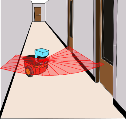
Ground vehicles come in variety of sizes and shapes depending on the objectives they have been designed for. Apart from structural differences, suite of sensors mounted on these robots depends on their operational environment. In indoor environments, GPS is not accessible but the environment is usually feature-rich due to surrounding walls, doors, furniture, etc. Thus, range sensors can be used to carry out scan matching (Kohlbrecher et al., 2013) in order to achieve accurate localization. Using stereo cameras is also an affordable solution to achieve depth data. Ring of ultrasonic sensors around the robot chassis is also a viable solution for obstacle detection (Kim and Kim, 2012) or localization (Moreno et al., 2002, 1999) in indoor environments. An illustration of indoor environment has been shown in figure 4. Regardless of being indoor or outdoor, INS can be used for localization which relies on IMU data. Indoor environments usually have smooth floors so wheel slippage is not likely and rotary encoders are quite suitable for estimating the robot displacement.

Figure 4. Indoor environment illustration.

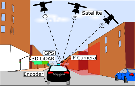
For outdoor environments, GPS can aid the absolute positioning provided that clear line-of-sight between the GPS receiver and at least four satellites is available. Such conditions may be violated in urban environments (figure 5a) due to signal blockage by tall buildings. However, urban environments are well-structured in nature. This property can be exploited to improve localization accuracy by performing scan matching on LiDAR data (Yang et al., 2018). Even if GPS signal is available, scan matching can still lead to better localization accuracy (Levinson et al., 2007). An alternate approach is visual place recognition (VPR) (Tomita et al., 2021; Chen et al., 2022a; Majdik et al., 2015) which plays a vital role in reducing localization error by recognizing the places that have been visited previously.

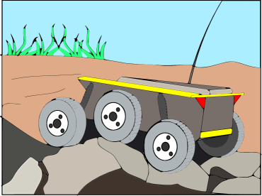
In some outdoor applications (e.g. military), the mobile robot encounters offroad environments which are harsh, unstructured, and sometimes impossible to traverse. Offroad environments push the mechanical (Ackerman, 2017) and autonomous capabilities (Jones et al., 2006) of mobile robots to their limits. As can be seen in figure 5b, the offroad robots must be equipped with large wheels, long travel suspension, and preferably all-wheel drive ability to be able to traverse different types of lands such as muddy, rocky, snowy, etc. Apart from robot mechanical requirements for offroad environments, several challenges must be addressed by autonomous software modules of the robot to achieve successful navigation:

1. Given that offroad environments do not follow any specific structure (Thakker et al., 2020), autonomous navigation cannot make any assumptions about them beforehand.

2. Some offroad environments like deserts are featureless which hinders localization of the robot due to lack of recognizable landmarks. For example in deserts, even the terrain shape may vary due to movement of sands by blowing winds.

3. The offroad environments are hazardous due to deep valleys, rough rivers, volcanoes, etc. Therefore, it is crucial to take into account impassable areas during path planning to enforce the robot safety.

4. In offroad environments, some of the obstacles may be passable like bushes while others are impassable like mountains. The ability to detect passable obstacles is vital to shorten the length of the planned path by moving through the passable obstacles.

5. Autonomous navigation relies on the robot sensor readings to make decisions. However, the field of view of sensors may be limited due to dense vegetation which hinders efficient localization.

6. Depending on the offroad environment, the robot motion controller parameters must be tuned differently (Bradley and Bagnell, 2010). For example, the amount of force applied to the robot wheels in snowy environments is different from dirt lands.

(a)

(b)

Figure 5. Ground robots for outdoor scenarios: (a) structured urban environment, (b) unstructured offroad environment.

3.2. Unmanned aerial vehicles

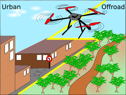
While controlling ground vehicles are simpler than unmanned aerial vehicles (UAVs), their movement is limited to traversable ground. Aerial vehicles are not bound to such constraints and they can reach the desired location in less time compared to ground vehicles. However, aerial vehicles have some limitations as well. For example, the flight duration may be short, especially for low-grade UAVs. Additionally, failure in control module may lead to a disastrous crash damaging the UAV. Another drawback is limited payload. UAVs can carry limited load which means the set of hardware (e.g. sensors and processing units) mountable on them must be chosen wisely. Given that IMUs are usually small and lightweight, using them to implement INS for efficient localization of UAVs is quite popular. As shown in figure 6a, UAVs may be deployed to variety of outdoor environments e.g. urban or unstructured and offroad. To keep the INS error bounded, GPS sensor can be mounted on UAVs (Nemra and Aouf, 2010; Abdelkrim et al., 2008; da Silva and da Cruz, 2016; Zhang and Hsu, 2018). Using UAVs in indoor environments is also possible. The only difference to outdoor scenarios is unavailability of GPS signals. Instead of GPS, INS data can be fused with LiDAR (Li et al., 2014), mix of laser data and vision sensors (Kara Mohamed et al., 2011), Ultra Wideband (UWB) (Song and Hsu, 2021), mix of UWB and 3D LiDAR (Li et al., 2016). Even seamless switch between indoor/outdoor navigation modes for UAVs has been attempted (Cebrian et al., 2019). Moreover, Hall effect sensor data has been used to aid the velocity update of INS (Zahran et al., 2019). Hall effect sensor detects magnetic filed presence and magnitude by exploiting Hall effect. According to this effect, a magnetic field perpendicular to current in an electrical conductor produces voltage difference across the electrical conductor such that it is transverse to the electric current and the magnetic field.

3.3. Underwater vehicles

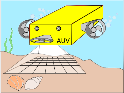
AUVs can be used in various applications such as retrieving black boxes of airplanes (Jian et al., 2015; Ridao et al., 2015) crashed in oceans/seas, enforcing security of ports and harbors by detection and disposal of explosives and mines (Abreu and Matos, 2014; Reed et al., 2010), and infrastructure maintenance for oil and gas industries (Xiang et al., 2010; Zhang et al., 2021; Calvo et al., 2009; Jacobi and Karimanzira, 2013). However, underwater autonomous navigation (figure 6b) is challenging due to unavailability of GPS (González-García et al., 2020) and limited visibility. Failing to register the current position of the robot using visual features leads to inaccurate localization which in turn hinders autonomous navigation (Qin et al., 2022). Using DR and INS to localize AUVs has a long history (Leonard et al., 1998). However, these methods suffer from accumulated error due to noisy sensor data, ocean currents, and Earth’s gravity in underwater environments (González-García et al., 2020). To deal with the accumulated error, Geophysical Navigation (GN) (Rice et al., 2004) can be used in which AUV sensor readings are matched with geophysical map of the underwater environment. Unfortunately, GN suffers from some drawbacks such as requiring geophysical map of the environment before the navigation starts and computational complexity of matching sensor data with the map. As an alternative approach to GN, acoustic ranging systems (Fallon et al., 2011) may be used but they rely on complex infrastructure and their cost of deployment is high. Researchers have explored new alternatives for AUV localization such as optical technologies (Bosch et al., 2016). Yet again, development of these technologies has been slowed down due to tough conditions of underwater environments. In the presence of proper lighting conditions, visual processing systems can improve localization accuracy significantly (González-García et al., 2020). For example, Mehdi et al. (Mehdi et al., 2021) have fused IMU and depth data extracted from stereo camera system to plot the map of the underwater environment using SLAM implemented in ROS. The map is used for path planning and autonomous navigation.

3.3.1. AUV suitable sensors

The first sensor to perform localization using INS underwater is IMU. To deal with INS accumulated error, fusing IMU data with other sensors is crucial. Doppler velocity loggers (DVL)(dop, [n. d.]) is a sonar system for measuring motion underwater that can determine the speed and the direction of AUV movement. Regarding absolute positioning, GPS cannot be used underwater since its electromagnetic signals decay quickly. Acoustic signaling is an alternative solution since acoustic signals decay very slowly underwater (He et al., 2011). The downside of this method is its reliance on baseline stations deployed in the navigation environment. The baseline batteries need frequent charging in order to stay functional and respond to interrogator device mounted on AUV. In addition, baseline deployment and recovery is time-consuming and costly which makes acoustic navigation impractical in large-scale environments (Kinsey et al., 2006). To address this problem, MIT researchers have developed underwater backscatter localization (UBL) (Ghaffarivardavagh et al., 2020) which is a battery-free pinpointing system. Instead of emitting acoustic signals which require battery consumption, UBL reflects the modulated signals from its surrounding environment. This way, position information is provided without needing any battery-operated device. UBL takes the role of underwater GPS.

Family of sonar sensors such as forward looking sonars and side scan sonar (Key, 2000) is widely used for obstacle detection and localization underwater. Off-the-shelf underwater camera systems (Massot-Campos and Oliver-Codina, 2015) are also very common for extracting depth data based on stereo vision.

(a)

(b)

Figure 6. Outdoor (a) aerial and (b) under-water environments and their respective robots.

4. Simulation tools

To conduct research in the field of robotics, a suitable robotic platform is needed which is a combination of software and hardware components. During research process, various experiments are needed to be carried out. It is quite likely for these experiments to fail due to software and/or hardware module malfunction. Sometimes, these failures may damage the robot. On the other hand, performing experiments on real robots is tedious and time consuming. An alternative approach is to implement and test the robot software in simulation. This way, researchers will not have to worry about accidentally damaging robots and no hardware is needed to test an initial idea. Resetting the simulation scenario is also much easier than resetting the robot status in real world. In table 2, the characteristics of some of main robotic simulators have been provided (rob, [n. d.]).

While testing new ideas in simulation is beneficial, it is not the ultimate goal of robotic projects. Sooner or later, the simulated project must be evaluated on real robots. The drawback of using simulators is that for modeling the physical laws of the real world, some compromises may have been made. Therefore, the project tested in simulation may need some refinements and manual tuning to be ready for deployment on a real robot. Nevertheless, putting the time and effort into developing robotic projects in simulation before deployment on real robots is definitely worth it since it reduces development time and cost significantly. Among the existing simulators, some like Gazebo rely on high quality physics engines such as open dynamic engine (ODE) (ode, [n. d.]) to reduce the gap between simulated and real robots drastically. That is why many well known robotic companies provide their customers with simulation tools of their commercial robots in the form of software packages relying on ROS and Gazebo. ROS is a set of tools and software libraries specifically designed to facilitate robot application development. Using ROS, development time of robotic projects is drastically reduced due to the possibility to use high quality of-the-shelf software packages that implement famous algorithms and interface with various sensors (hardware abstraction). Some examples of well-known robots with descent simulation in ROS and Gazebo include but are not limited to Fetch robotics (fet, [n. d.]), PR2 robot (pr2, [n. d.]), KUKA iiwa (kuk, [n. d.]a), and humanoid Nao robot (nao, [n. d.]).

Table 2. Characteristics comparison of main robotic simulators

Simulator	Supported OS	Physics engine	ROS support	Supported
				Robots	Actuators	Tools	Sensors
Gazebo(gaz, [n. d.])	Linux	ODE, Bullet, Simbody, DART	ROS1, ROS2	Mobile, humanoid, industrial	Revolute, prismatic, screw and spherical joints	Grippers	Camera, distance & proximity sensors, laser, force sensors
RoboDK	Linux, Mac OS, Windows, Android	None	-	Industrial robots	Possibility to create rotated and linear axis	Grippers, weld tools, spindle, grinding, polishing, tool changer, …	Lasers, cameras, laser tracker
Webots(web, [n. d.])	Linux, Mac OS, Windows	Proprietary, ODE-based	ROS1, ROS2	Mobile, humanoid, industrial	Brake, connector, display, emitter, linear/rotational motor, muscle, pen, propeller, speaker, track (conveyor belt or tank robots)	Grippers	Accelerometer, camera, compass, distance sensor, GPS, gyroscope, lidar, position sensor, receiver, touch sensor
CoppeliaSim (cop, [n. d.])	Linux, Mac OS, Windows	ODE, Bullet, Vortex, Newton	ROS1, ROS2	Mobile, humanoid, industrial	Revolute, prismatic & spherical motors	Pens, paint gun, welding torch, grippers	Vision, force sensors, proximity sensor, accelerometer, gyroscope, lasers, LiDARs
OpenRave	Linux, Windows	ODE, Bullet	ROS1	Mobile, humanoid, industrial	Revolute & linear joints	Grippers	Cameras, ray-casting laser
Unity	Linux, Mac OS, Windows	NVidia PhysX, Box2D, other open-source physics engines	ROS1, ROS2	Mobile, humanoid, industrial	Revolute & prismatic joints	Grippers	Cameras

5. Path planning

After percepting the environment using robot onboard sensors, it is necessary to plan a feasible path in order to reach the desired target starting from the current position. The choice of the path planning algorithm depends on whether the environment map is available or not. In case the map is known, the choice of the path planner depends on the map representation. For occupancy grid maps, D* (Stentz, 1997) and its extensions such as focused D* (Stentz et al., 1995) and D* Lite (Koenig and Likhachev, 2005) are suitable choices. D* and its extensions are all considered as incremental search algorithms. D* assumes that unseen parts of the environment are free of obstacles. Based on this assumption, D* uses the map to compute the shortest path from the start to the goal. In the event of observing new obstacles, the map is updated with their information and a new shortest path is computed if necessary. This trend repeats until the goal is reached or it is concluded that the goal is indeed unreachable. Considering that observing new obstacles during navigation is quite likely, recomputing the shortest path must be fast which is what D* and its extensions are famous for. It is worth noting that focused D* is a combination of A* (Hart et al., 1968) and the ideas from the original D* algorithm; and D* Lite has been built based on life long planning A* (LPA*)(Koenig et al., 2004) and another incremental search method made of combining A* ideas and dynamic SWSF-FP (Ramalingam and Reps, 1996).

5.1. DMP-based path planning

One of the popular approaches for trajectory planning and control signals generation in manipulator robots is dynamic movement primitive (DMP) (Schaal, 2006; Ijspeert et al., 2013). DMP is a highly adaptable mathematical model capable of representing complex trajectories without the need for manual tuning of its parameters. Roughly speaking, a DMP is a second order nonlinear dynamical system capable of imitating complex trajectories provided that its parameters are set appropriately. DMPs are either discrete or rhythmic which are suitable for generation of aperiodic and periodic trajectories, respectively. Discrete DMPs are suitable for path following since planned paths are not periodic trajectories. The crux of a discrete DMP is a point-attractor system:

(1) $$\ddot{y}=\alpha_{y}\left[\beta_{y}(g-y)-\dot{y}\right],$$

where $y$, $\dot{y}$, and $\ddot{y}$ are the system position, velocity, and acceleration, respectively. Moreover, $g$ is the goal point and $\alpha_{y}>0$ and $\beta_{y}>0$ are gain coefficients. Careful inspection of equation 1 reveals that it is just a PD controller whose objective is to reach $g$ given the current state $y$. To specify the shape of the trajectory between $y$ and $g$, equation 1 is augmented with a special function $f(x)$ known as the forcing function(Schaal, 2006):

(2) $$f(x)=\frac{\sum_{i=1}^{N}\psi_{i}w_{i}}{\sum_{j=1}^{N}\psi_{j}}(g-y_{0})x,$$

where $\psi_{i}$ is the ith Gaussian basis function, $w_{i}$ is the ith weight parameter, $y_{0}$ is the initial position of the system and $x$ is state variable of another dynamical system known as the canonical system. By setting the parameter set $\{w_{i},i=1,...,N\}$ of the forcing function, any arbitrary trajectory can be produced using DMP. The canonical system

(3) $$\zeta\dot{x}=-\alpha_{x}x,$$

controls the life time of the DMP. In equation 3, $\alpha_{x}$ is a constant which is set to $-\log(0.01)$ for ensuring 99% convergence of the DMP after its life time $\zeta$ is passed.

Despite the fact that DMP is primarily designed for motion planning of robotic manipulators, it has also been used for path planning in mobile robots. For example, Jiang et al. (Jiang et al., 2016) have carried out mobile robot path planning using DMPs. A desired path is first planned and trajectories are extracted from it to be used as training samples for adjustment of DMP parameters. Thanks to the DMP high adaptability, Jiang et al. were able to achieve smooth trajectories for the mobile robot even when start and goal positions were altered.

6. Path following

To execute planned paths, mobile robots must be equipped with the necessary means to follow them. Over the years, various path following methods have been developed. Some of these methods are as simple as pure pursuit while others take a more involved approach by relying on dynamical systems or deep learning. Some of these path following methods are reviewed in this section.

6.1. Pure pursuit algorithm

Pure pursuit (Coulter, 1992) is a path tracking algorithm with respectable history as it has been used in various projects such as the Terragator (Champeny-Bares et al., 1991), NavLab(Thorpe et al., 1989), and NavLabs2(Coulter and Mueller, 1994). In a nutshell, pure pursuit algorithm computes the robot angular velocity while assuming constant linear velocity. The robot is moved from its current position to some look-ahead point in front of it. After reaching the specified look-ahead point, it is moved further on the path which is to be followed.

The algorithm computes an arc joining the robot current position to the goal position. The goal point is one look-ahead distance from the current position of the robot. In figure 7, the robot’s local coordinate frame as well as the goal point $(x_{g},y_{g})$ have been shown. The objective is to compute the curvature $\gamma$ of the arc joining the robot current position to the goal position assuming chord length (look-ahead distance) of $1$. The goal point is enforced to be on the robot path.

Figure 7. Geometry of the pure pursuit algorithm: $1$ is the chord length (look-ahead distance), $r$ is the radius of the arc joining robot position to the goal point, $(x_{g},y_{g})$ is the goal point

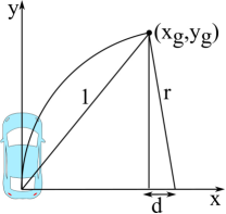
Computation of the curvature value is fairly straightforward. Looking at figure 7, one can write the following equations:

(4) $$x^{2}+y^{2}=1^{2}$$

(5) $$x+d=r$$

where equation 4 follows from Pythagorean theorem in the left bigger triangle and equation 5 is due to the fact that sum of x and d is equal to the radius of curvature $r$. Using equations 4 and 5, the curvature $\gamma$ can be computed as:

$$d=r-x$$

(6) $$(r-x)^{2}+y^{2}=r^{2}\implies r^{2}-2rx+x^{2}+y^{2}=r^{2}\implies 2rx=l^{2}\implies r=\frac{l^{2}}{2x}\implies\gamma=\frac{2x}{l^{2}}$$

6.2. DMP-based path following

As mentioned in section 5, DMP is a popular tool that generates smooth trajectories for manipulator robots. However, it has also been used for path following of mobile robots. Sharma el al.(Sharma et al., 2019) have implemented a DMP-based path tracking approach for nonholonomic robots which is capable of avoiding an obstacle on the path. Two DMPs (to represent movement along x and y axes) were used and forcing function of each of the DMPs was parameterized using radial basis functions (RBFNs). Thanks to the adaptive nature of DMP, the proposed approach can preserve the shape of the planned trajectory and reach the goal even if the start or goal position is altered. Moreover, the proposed approach is able to suggest both trajectories passing both sides of the obstacle. This is particularly useful when one of the two paths is not traversable for some reason.

6.3. DL and RL-based path following

Inspired by interesting learning results achieved by RL, it has been extended to handle problems with continuous state and action spaces. This trend has been reinforced by borrowing ideas from DL giving birth to robust deep RL (DRL) methods capable of controlling robots with continuous and high dimensional states and action spaces. For example, Cheng et al. (Cheng et al., 2022) applied DRL for path following and obstacle avoidance. The path following is realized by designing appropriate state and reward functions which are central to successful training of any RL agent. To realize obstacle avoidance, the aforementioned reward and state functions are modified to take into account distance and angle to detect obstacles. The RL algorithm used in this work was DDPG (Lillicrap et al., 2015). The proposed approach has been evaluated in simulation.

7. Sensor fusion methods

Effective localization of mobile robots is a challenging task. There are multiple sources of uncertainty that the localization module has to deal with in order to estimate robot location with reasonable accuracy at each instance in time. The simplest form of localization is dead reckoning (DR) (Choset et al., 2005). In this method, equations of motion of the mobile robot are devised based on robot structural properties such as wheel circumference, onboard sensors e.g. IMU, magnetometer, and rotary encoders. Knowing number of wheel rotations (using rotary encoder) and direction of movement, it is possible to estimate the robot position and heading at each instance in time. However, sensor readings are always noisy so estimated positions are prone to errors. The situation gets worse by stochastic phenomena of the surrounding environment. For example, in case of wheel slippage, the rotary encoder reports wheel movement, however, due to slippage the robot may not have move at all leading to incorrect position estimation. To deal with localization error, it is common practice to fuse readings from multiple sensors to get a better position estimation. In the remainder of this section, some of the most famous filtering algorithms that are used in mobile robot localization are reviewed.

7.1. Kalman filter

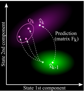
Kalman filter (KF) is an algorithm for estimation of unknown variables based on a sequence of possibly noisy observations (measurements) collected over time. The estimated values will be more precise compared to the values estimated based on a single observation. KFs do not keep history of past observations. Only the previous state is kept so memory requirements are light. KFs computations are fast enough to be used in real-time applications such as robot localization. KF models the unknown current state vector $x_{k-1}$ with a Gaussian distribution $\mathcal{N}(\hat{x}_{k-1},P_{k-1})$ in which $k-1$ is the current time step, $\hat{x}_{k-1}$ and $P_{k-1}$ are the mean and covariance matrix of the distribution. The hat accent of $\hat{x}_{k-1}$ emphasizes that mean is not necessarily equal to the true current state $x_{k-1}$. The motivation for this representation is that the true state $x_{k-1}$ is not known but some states are more likely than others and the elements of the state vector may be correlated. These two properties are captured by the Gaussian distribution covariance matrix. KF cycles through prediction and correction phases. In the prediction phase, the linear equations governing the robot motion are represented as matrix $F_{k}$ which can be multiplied with the current state estimate $\hat{x}_{k-1}$ to predict the next state $\hat{x}_{k}$. However, the effect of external control commands (or forces) such as turning the wheel or stopping must be taken into account as well. In KF terminology, the control vector is denoted as $u_{k}$. How $u_{k}$ affects the next state is represented by matrix $B_{k}$. The final equation for predicting next state using KF reads as:

(7) $${\color[rgb]{1,0,1}\definecolor[named]{pgfstrokecolor}{rgb}{1,0,1}\pgfsys@color@cmyk@stroke{0}{1}{0}{0}\pgfsys@color@cmyk@fill{0}{1}{0}{0}\hat{x}_{k}}=F_{k}{\color[rgb]{0,0,0}\definecolor[named]{pgfstrokecolor}{rgb}{0,0,0}\hat{x}_{k-1}}+B_{k}u_{k}.$$

It is also necessary to update the covariance matrix $P_{k}$. This is done using matrix $F_{k}$. However, the uncertainty due to external events such as robot wheel slippage or wind force (for aerial robots) must be considered as well. KF models external uncertainty by mapping each point from the current Gaussian $\mathcal{N}(\hat{x}_{k-1},P_{k-1})$ to multiple new points which will be part of the next Gaussian distribution $\mathcal{N}(\hat{x}_{k},P_{k})$. The external uncertainty is captured by adding covariance matrix $Q_{k}$ to the update equation of $P_{k}$ yielding:

(8) $${\color[rgb]{1,0,1}\definecolor[named]{pgfstrokecolor}{rgb}{1,0,1}\pgfsys@color@cmyk@stroke{0}{1}{0}{0}\pgfsys@color@cmyk@fill{0}{1}{0}{0}P_{k}}=F_{k}{\color[rgb]{0,0,0}\definecolor[named]{pgfstrokecolor}{rgb}{0,0,0}P_{k-1}}F_{k}^{T}+Q_{k},$$

which means the new estimate of $P_{k}$ is computed from the current estimate $P_{k-1}$ and additional environment uncertainty represented by $Q_{k}$. The prediction process is graphically illustrated in figure 8a.

(a)

(b)

(c)

Figure 8. Kalman filter phases for 2D state vector: (a) prediction phase, (b) expected observation computation based on predicted state $\hat{x}_{k}$, (c) correction phase.

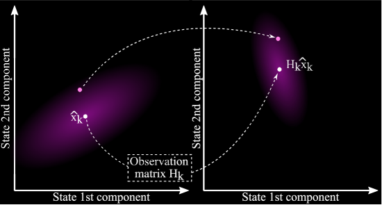
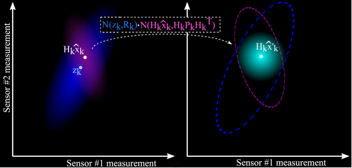
In the correction phase, the expected observations (i.e. expected sensor readings) are computed by multiplying matrix $H_{k}$ with the new estimates $\{\hat{x}_{k},P_{k}\}$ (figure 8b). Actual observations are also obtained from the onboard sensors.

Therefore, the overlap of Gaussian distributions $\mathcal{N}(H_{k}\hat{x}_{k},H_{k}P_{k}H_{k}^{T})$ and $\mathcal{N}(z_{k},R_{k})$ can be computed to obtain the corrected observation distribution with mean $H_{k}\hat{x}_{k}^{\prime}$ as shown in figure 8c. After some manipulation, the $H_{k}$ in front of $H_{k}\hat{x}_{k}^{\prime}$ can be dropped to get the final equations for correcting the prediction ($\{\hat{x}_{k},P_{k}\}$):

$${\color[rgb]{0,0,0}\definecolor[named]{pgfstrokecolor}{rgb}{0,0,0}\hat{x}_{k}^{\prime}}={\color[rgb]{1,0,1}\definecolor[named]{pgfstrokecolor}{rgb}{1,0,1}\pgfsys@color@cmyk@stroke{0}{1}{0}{0}\pgfsys@color@cmyk@fill{0}{1}{0}{0}\hat{x}_{k}}+{\color[rgb]{0,0,0}\definecolor[named]{pgfstrokecolor}{rgb}{0,0,0}K_{k}}\left({\color[rgb]{0,0,1}\definecolor[named]{pgfstrokecolor}{rgb}{0,0,1}z_{k}}-H_{k}{\color[rgb]{1,0,1}\definecolor[named]{pgfstrokecolor}{rgb}{1,0,1}\pgfsys@color@cmyk@stroke{0}{1}{0}{0}\pgfsys@color@cmyk@fill{0}{1}{0}{0}\hat{x}_{k}}\right),$$

$${\color[rgb]{0,0,0}\definecolor[named]{pgfstrokecolor}{rgb}{0,0,0}P^{\prime}_{k}}={\color[rgb]{1,0,1}\definecolor[named]{pgfstrokecolor}{rgb}{1,0,1}\pgfsys@color@cmyk@stroke{0}{1}{0}{0}\pgfsys@color@cmyk@fill{0}{1}{0}{0}P_{k}}-{\color[rgb]{0,0,0}\definecolor[named]{pgfstrokecolor}{rgb}{0,0,0}K_{k}}H_{k}{\color[rgb]{1,0,1}\definecolor[named]{pgfstrokecolor}{rgb}{1,0,1}\pgfsys@color@cmyk@stroke{0}{1}{0}{0}\pgfsys@color@cmyk@fill{0}{1}{0}{0}P_{k}},$$

$${\color[rgb]{0,0,0}\definecolor[named]{pgfstrokecolor}{rgb}{0,0,0}K_{k}}={\color[rgb]{1,0,1}\definecolor[named]{pgfstrokecolor}{rgb}{1,0,1}\pgfsys@color@cmyk@stroke{0}{1}{0}{0}\pgfsys@color@cmyk@fill{0}{1}{0}{0}P_{k}}H_{k}^{T}\left(H_{k}{\color[rgb]{1,0,1}\definecolor[named]{pgfstrokecolor}{rgb}{1,0,1}\pgfsys@color@cmyk@stroke{0}{1}{0}{0}\pgfsys@color@cmyk@fill{0}{1}{0}{0}P_{k}}H_{k}^{T}+{\color[rgb]{0,0,1}\definecolor[named]{pgfstrokecolor}{rgb}{0,0,1}R_{k}}\right)^{-1},$$

where $R_{k}$ is the covariance matrix describing sensors uncertainty and $K_{k}$ is known as the Kalman gain.

7.2. Extended Kalman filter

KF is a powerful state estimator even in the presence of noisy sensor readings. However, to be able to use KF, the state propagation equations must be linear. This requirement rarely holds in real-world applications. Even in the case of a simple differential drive robot (compiled from Dudek and Jenkin, [n. d.]), the kinematics equations are nonlinear. That is where the extended Kalman filter (EKF) (Welch et al., 1995) comes in. The main idea behind EKF is to linearize nonlinear state propagation equations using Jacobian (matrix of partial derivatives) so that the propagation equations can be expressed as equation 7. To this end, partial derivatives of the next state $\hat{x}_{k}$ are computed with respect to the current state $\hat{x}_{k-1}$ yielding matrix $F_{k}$ and partial derivatives of the next state $\hat{x}_{k}$ with respect to the control vector $u_{k}$ are computed yielding matrix $B_{k}$:

$$F_{k}=\begin{bmatrix}\frac{\partial\hat{x}_{k,1}}{\partial\hat{x}_{k-1,1}}&\ldots&\frac{\partial\hat{x}_{k,1}}{\partial\hat{x}_{k-1,n}}\\ \vdots&\ddots&\vdots\\ \frac{\partial\hat{x}_{k,n}}{\partial\hat{x}_{k-1,1}}&\ldots&\frac{\partial\hat{x}_{k,n}}{\partial\hat{x}_{k-1,n}}&\end{bmatrix},\quad B_{k}=\begin{bmatrix}\frac{\partial\hat{x}_{k,1}}{\partial u_{k,1}}&\ldots&\frac{\partial\hat{x}_{k,1}}{\partial u_{k,m}}\\ \vdots&\ddots&\vdots\\ \frac{\partial\hat{x}_{k,n}}{\partial u_{k,1}}&\ldots&\frac{\partial\hat{x}_{k,n}}{\partial u_{k,m}}&\end{bmatrix},$$

where state vectors are assumed to be n-dimensional. Following a similar pattern, nonlinear equations for mapping predicted next state $\hat{x}_{k}$ to predicted observations $\hat{z}$ are linearized using partial derivatives of observations (sensor readings) with respect to $\hat{x}_{k}$:

(9) $$H_{k}=\begin{bmatrix}\frac{\partial\hat{z}_{k,1}}{\partial\hat{x}_{k,1}}&\ldots&\frac{\partial\hat{z}_{k,1}}{\partial\hat{x}_{k,n}}\\ \vdots&\ddots&\vdots\\ \frac{\partial\hat{z}_{k,h}}{\partial\hat{x}_{k,1}}&\ldots&\frac{\partial\hat{z}_{k,h}}{\partial\hat{x}_{k,n}}&\end{bmatrix},$$

where observation vector is assumed to be h-dimensional.

7.3. Unscented Kalman Filter

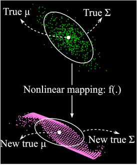
As mentioned in section 7.2, EKF tackles the nonlinear system equations using their first order approximations. In practice, this linearization method may lead to a posterior distribution with corrupted mean and covariance. This issue has been addressed by Unsented Kalman Filter (UKF) (Wan et al., 2001) via taking a derivative-free approach based on deterministic sampling. Instead of employing a Gaussian, UKF represents the state distribution by carefully choosing a set of sample points around the distribution mean. These points are known as the sigma points $\{\sigma^{(k-1)}_{i},i=1,...,2n+1\}$ where $n$ is the dimension of the state vector and $k-1$ refers to the current time step. As pointed out in (Wan et al., 2001), the sigma points are selected as:

$$\sigma^{(k-1)}_{0}=\hat{x}_{k-1},$$

$$\sigma^{(k-1)}_{i}=\hat{x}_{k-1}{\color[rgb]{0,0,1}\definecolor[named]{pgfstrokecolor}{rgb}{0,0,1}+}\left(\sqrt{(n+\lambda)P_{k-1}}\right)_{{\color[rgb]{0,0,1}\definecolor[named]{pgfstrokecolor}{rgb}{0,0,1}i}},\quad i=1,...,n,$$

$$\sigma^{(k-1)}_{i}=\hat{x}_{k-1}{\color[rgb]{0,0,1}\definecolor[named]{pgfstrokecolor}{rgb}{0,0,1}-}\left(\sqrt{(n+\lambda)P_{k-1}}\right)_{{\color[rgb]{0,0,1}\definecolor[named]{pgfstrokecolor}{rgb}{0,0,1}i-n}},\quad i=n+1,...,2n$$

where $\lambda$ is a scaling parameter and $\left(\sqrt{(n+\lambda)P_{k-1}}\right)_{i}$ refers to the i-th column of matrix square root of $(n+\lambda)P_{k-1}$. The square root may be computed e.g. by lower triangular Cholesky factorization.

Similar to KF, UKF workflow includes prediction and correction phases followed by a new phase for sigma points selection. Assuming that the next state $\hat{x}_{k}$ is calculated as nonlinear mapping $f(.)$ of the current state $\hat{x}_{k-1}$, in the prediction phase, the sigma points undergo unscented transform (Julier and Uhlmann, 1997) by being fed to the nonlinear function $f(.)$:

$$\sigma^{(k)}_{i}=f(\sigma^{(k-1)}_{i}),\quad i=1,...,2n+1.$$

The weighted average of the new sigma points are then used to estimate the mean and covariance of the predicted state:

$$\hat{x}_{k}\simeq\sum_{i=1}^{2n+1}w_{i}^{(m)}\sigma^{(k)}_{i},$$

$$P_{k}\simeq\sum_{i=1}^{2n+1}w_{i}^{(c)}\left(\sigma^{(k)}_{i}-\hat{x}_{k}\right)\left(\sigma^{(k)}_{i}-\hat{x}_{k}\right)^{T}.$$

The transformed sigma points are then used to calculate the mean and covariance of the new state Gaussian distribution. The estimated mean and covariance are accurate up to the second order of Taylor series expansion (Wan et al., 2001).

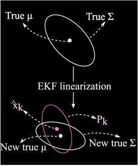
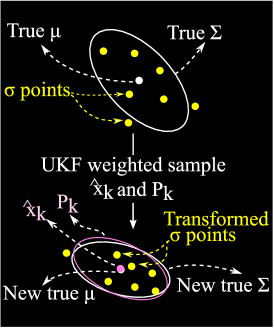
The difference between EKF and UKF state propagation mechanism has been depicted in figure 9. Given the current distribution with mean $\mu$ and covariance $\Sigma$, in the absence of noise, applying nonlinear mapping $f(.)$ yields the new mean and covariance (figure 9a). The drawback of EKF linearization is apparent in figure 9b. The error introduced by the first order linearization has led to mismatch between true ($\mathcal{N}(\mu_{New},\Sigma_{New})$) and predicted ($\mathcal{N}(\hat{x}_{k},P_{k})$) distributions. The distribution mismatch has been addressed by UKF in figure 9c. To this end, multiple sigma points sampled from the current distribution have been transformed based on $f(.)$. The transformed points are then used to calculate the new mean and covariance. Such an approach is more flexible and reliable compared to EKF first order linearization.

(a) True mapping

(b) EKF prediction

(c) UKF prediction

Figure 9. Illustrating the state propagation mechanisms of EKF and UKF compared to the true mapping.

7.4. Multi-State Constraint Kalman Filter

Inertial navigation system (INS) is the backbone of autonomous navigation that can be applied on aerial (Sayre-McCord et al., 2018; Geneva et al., 2020; Morales and Kassas, 2021), ground (Lobo et al., 1995; Cai et al., 2019; Chae et al., 2020), and underwater vehicles (Hegrenas et al., 2008; Hegrenaes and Berglund, 2009; Bao et al., 2020). Relying primarily on IMU, INS provides very cost-efficient navigation solution. However, INS localization accuracy degrades over time due to accumulative error. INS employs numerical integration over gyroscope and accelerometer readings to estimate the position and orientation of the platform it is mounted on. Applying numerical integration in successive time steps causes the aforementioned accumulated error. That is why INS is usually paired with auxiliary sensor(s) e.g. GPS, magnetometer, camera, etc. for error correction. The choice of the auxiliary sensors depends on the characteristics of the environment (e.g. indoor/outdoor, in the air/on the ground/underwater).

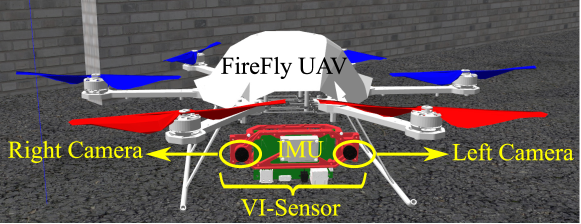
Visual sensors such as cameras can be used in variety of environments and they are available at reasonable prices. That is the motivation behind Multi-State Constraint Kalman Filter (MSCKF) which is an EKF-based method designed to implement visually-aided inertial navigation in real-time (Mourikis et al., 2007). The main difference between MSCKF and ordinary EKF is the fact that MSCKF uses a novel measurement model capable of capturing geometric constraints that arise when a static feature appears in multiple cameras with different poses. Thanks to this new measurement model, MSCKF is able to perform localization which is accurate up to linearization error of EKF only using visual sensor(s). Moreover, MSCKF computational complexity scales linearly with the number of features which is remarkable. One of the notable applications of MSCKF is visual-inertial navigation system OpenVINS implemented by Geneva et al. (Geneva et al., 2020) which utilizes a VI-sensor (visual-inertial sensor) similar to the one shown in figure 10. The VI-sensor consists of two cameras and one 3-axis IMU which are hardware-synchronized.

The goal of MSCKF is 3D pose estimation of reference frame $\{I\}$ of an IMU strapped to a mobile (robot) platform with respect to some global reference frame $\{G\}$. To this end, the IMU state is written as (Mourikis et al., 2007):

(10) $$X_{IMU}=\left[{}^{I}_{G}\bar{q}^{T},b_{g}^{T},{}^{G}v^{T}_{I},b_{a}^{T},{}^{G}p^{T}_{I}\right]^{T},$$

where the rotation from global frame $\{G\}$ to IMU frame $\{I\}$ is expressed as a unit quaternion ${}^{I}_{G}\bar{q}^{T}$. Moreover, ${}^{G}v^{T}_{I}$ and ${}^{G}p^{T}_{I}$ represent the IMU position and velocity with respect to $\{G\}$, and the $3\times 1$ vectors $b_{g}$ and $b_{a}$ express the gyroscope and accelerometer bias affecting their measurements. Based on equation 10, the error state of the IMU reads as (Mourikis et al., 2007):

(11) $$\tilde{X}_{IMU}=\left[\delta\theta_{I}^{T},\tilde{b}_{g}^{T},{}^{G}\tilde{v}^{T}_{I},\tilde{b}_{a}^{T},{}^{G}\tilde{p}^{T}_{I}\right]^{T},$$

where the additive error definition (i.e. difference between true value and estimated value) is used to compute error for position, velocity, and biases but the orientation error is described by the error quaternion $\delta\bar{q}$ such that the relation $\bar{q}=\delta\bar{q}\otimes\hat{\bar{q}}$ holds in which $\otimes$ stands for quaternion multiplication.

As the objective of MSCKF is an accurate estimation of IMU pose and orientation, the IMU state (equation 10) is used as part of the EKF state vector (Mourikis et al., 2007):

(12) $$\hat{X}_{k}=\left[\hat{X}_{IMU_{k}}^{T},{}^{C_{1}}_{G}\hat{\bar{q}}^{T},{}^{G}\hat{p}^{T}_{C_{1}},...,{}^{C_{N}}_{G}\hat{\bar{q}}^{T},{}^{G}\hat{p}^{T}_{C_{N}}\right]^{T},$$

where subscript $k$ in $\hat{X}_{k}$ denotes the EKF state at time step $k$. In addition to the IMU state, equation 12 contains $N$ pairs of $\{{}^{C_{i}}_{G}\hat{\bar{q}}^{T},{}^{G}\hat{p}^{T}_{C_{i}}\}$ items where ${}^{C_{i}}_{G}\hat{\bar{q}}^{T}$ is the quaternion expressing the rotation from the i-th camera frame $\{C_{i}\}$ to the global frame and ${}^{G}\hat{p}^{T}_{C_{i}}$ denotes the origin of frame $\{C_{i}\}$ expressed in the global frame. The aforementioned pairs corresponding to $N$ cameras are considered in the EKF state to establish geometric constraints induced by observation of static features from multiple cameras poses. Looking at equation 12, the EKF error-state vector reads as (Mourikis et al., 2007):

(13) $$\tilde{X}_{k}=\left[\tilde{X}_{IMU_{k}}^{T},\delta\theta_{C_{1}}^{T},{}^{G}\tilde{p}^{T}_{C_{1}},...,\delta\theta_{C_{N}}^{T},{}^{G}\tilde{p}^{T}_{C_{N}}\right]^{T},$$

where $\{\delta\theta_{C_{i}}^{T},{}^{G}\tilde{p}^{T}_{C_{i}}\}$ expresses the i-th camera attitude and position error.

Recall that EKF consists of prediction and correction phases. In the prediction phase, the IMU state (i.e. position and attitude of frame $\{I\}$) is propagated according to the set of equations that will be described below.

The first equation expresses how quaternion ${}^{I}_{G}\hat{\bar{q}}$ evolves over time (Mourikis et al., 2007):

(14) $${}^{I}_{G}\dot{\hat{\bar{q}}}=\frac{1}{2}\Omega(\hat{\omega}){}^{I}_{G}\hat{\bar{q}},$$

where ${}^{I}_{G}\dot{\hat{\bar{q}}}$ is the derivative of quaternion $\bar{q}$ at time step $t$ and matrix $\Omega(\hat{\omega})$ is computed as (Mourikis et al., 2007):

(15) $$\Omega(\hat{\omega})=\begin{bmatrix}-\lfloor\hat{\omega}\times\rfloor&\hat{\omega}\\ -\hat{\omega}^{T}&0\end{bmatrix}.$$

In equation 15, $\hat{\omega}=\omega_{m}-\hat{b}_{g}-C({}^{I}_{G}\hat{\bar{q}})\omega_{G}$ where $\omega_{m}$ is the gyroscope sensor reading from which $\hat{b}_{g}$ and $C({}^{I}_{G}\hat{\bar{q}})\omega_{G}$ are subtracted to cancel the effect of gyroscope bias and angular rate $\omega_{G}$ caused by planet’s rotation, respectively. Note that the term $C({}^{I}_{G}\hat{\bar{q}})$ represents the rotational matrix corresponding to quaternion ${}^{I}_{G}\hat{\bar{q}}$. The other component of matrix $\Omega(\hat{\omega})$ (equation 15) is $-\lfloor\hat{\omega}\times\rfloor$ which is known as the skew symmetric matrix of angular velocity vector $\hat{\omega}=[\hat{\omega}_{x},\hat{\omega}_{y},\hat{\omega}_{z}]^{T}$ (Titterton et al., 2004). The second and third equations of IMU state propagation express the evolution of gyroscope and accelerometer biases ($\dot{\hat{b}}_{g},\dot{\hat{b}}_{a}$) over time (Mourikis et al., 2007):

(16) $$\dot{\hat{b}}_{g}=\mathbb{E}\left[n_{g}\right]=[0,0,0]^{T},\>\dot{\hat{b}}_{a}=\mathbb{E}\left[n_{a}\right]=[0,0,0]^{T},$$

where $n_{g}$ and $n_{a}$ are the gyroscope and accelerometer biases, respectively and they are modeled as zero-mean white Gaussian noise processes. That is why expectation of $n_{g}$ and $n_{a}$ are zero vectors as shown in equation 16. The fourth equation related to IMU state propagation reads as (Mourikis et al., 2007):

(17) $${}^{G}\dot{\hat{v}}_{I}=C({}^{I}_{G}\hat{\bar{q}})^{T}\hat{a}-2\lfloor\omega_{G}\times\rfloor{}^{G}\hat{v}_{I}-\lfloor\omega_{G}\times\rfloor^{2}\>{}^{G}\hat{p}_{I}+G_{g},$$

where ${}^{G}\dot{\hat{v}}_{I}$ is the derivative of IMU frame velocity which expresses the IMU frame acceleration with respect to frame $\{G\}$. Moreover, $\hat{a}=a_{m}-\hat{b}_{a}$ where $a_{m}$ is the accelerometer sensor reading from which the accelerometer bias $\hat{b}_{a}$ is subtracted. The term $\lfloor\omega_{G}\times\rfloor$ in equation 17 is the skew symmetric matrix corresponding to planet’s rotation $\omega_{G}$ and as mentioned before, ${}^{G}\hat{v}_{I}$ and ${}^{G}\hat{p}_{I}$ represent the IMU frame velocity and position with respect to frame $\{G\}$ and $G_{g}$ stands for gravitational acceleration expressed in frame $\{I\}$. The last equation for IMU state propagation establishes the relation between the IMU velocity and position (Mourikis et al., 2007):

(18) $${}^{G}\dot{\hat{p}}_{I}={}^{G}\hat{v}_{I}.$$

To sum up, the set of equations 14-17 form the basis of the prediction phase of MSCKF. Considering that MSCKF is based on EKF, it is necessary to linearize equations 14-17:

(19) $$\dot{\tilde{X}}_{IMU}=F\tilde{X}_{IMU}+G_{n_{IMU}},$$

where matrices $F$ and $G_{n_{IMU}}$ are the results of linearizing equations 14-17 (see (Mourikis et al., 2007) for further details) and $n_{IMU}=\left[n_{g}^{T},n_{wg}^{T},n_{a}^{T},n_{wa}^{T}\right]^{T}$ is the system noise consisting of gyroscope and accelerometer noise densities ($n_{g},n_{a}$) and random walks ($n_{wg},n_{wa}$). The covariance matrix $Q_{IMU}$ corresponding to the system noise $n_{IMU}$ is computed during the calibration process offline. Kalibr (eth, [n. d.]c; Rehder et al., 2016; Furgale et al., 2013, 2012; Maye et al., 2013; Oth et al., 2013) is one of the famous calibration tools implemented in ROS which can be used to determine IMU noise density and random walk parameters as well as camera intrinsic and extrinsic parameters. Moreover, Kalibr offers spatial (coordinate transform) and temporal (time synchronization) calibration of an IMU with respect to a mono/stereo camera system.

As mentioned before, MSCKF exploits the presence of 3D features in multiple camera poses. To this end, the EKF state vector is augmented with the camera poses from which the 3D features are observed. The camera poses are determined based on the current estimate of the IMU pose. The EKF covariance matrix is updated as well.

To implement the correction phase of the EKF, a new measurement model is used. Consider a single feature $f_{j}$ which has been observed in $M_{j}$ camera poses. Then according to the measurement model, each of these $M_{j}$ observations is expressed as (Mourikis et al., 2007):

(20) $$z_{i}^{(j)}=\frac{1}{{}^{C_{i}}Z_{j}}\begin{bmatrix}{}^{C_{i}}X_{j}\\ {}^{C_{i}}Y_{j}\end{bmatrix}+n_{i}^{(j)},\quad i\in S_{j},$$

where $n_{i}^{(j)}$ is a $2\times 1$ vector expressing image noise and ${}^{C_{i}}p_{f_{j}}=\left[{}^{C_{i}}X_{j},{}^{C_{i}}Y_{j},{}^{C_{i}}Z_{j}\right]$ is the 3D position of the feature $f_{j}$ in i-th camera pose frame $\{C_{i}\}$. To determine ${}^{C_{i}}p_{f_{j}}$, the 3D position of the feature $f_{j}$ in global frame (${}^{G}p_{f_{j}}$) is needed which is unknown. To estimate ${}^{G}p_{f_{j}}$, lease-squares minimization is employed. The estimated vector ${}^{G}\hat{p}_{f_{j}}$ is used to compute estimated 3D position of the feature $f_{j}$ in frame $\{C_{i}\}$ (i.e. ${}^{C_{i}}p_{f_{j}}$) using the transformation from frame $\{G\}$ to frame $\{C_{i}\}$. Using ${}^{C_{i}}p_{f_{j}}$ and equation 20, the measurement model output (i.e. $\hat{z}_{i}^{(j)}$) can be computed. The difference between $\hat{z}_{i}^{(j)}$ and the measurement obtained from the environment ($z_{i}^{(j)}$) forms the measurement residual $r_{i}^{(j)}$ which is linearized to comply with EKF requirements. Gathering all residuals $\{r_{i}^{(j)},i=1,...,M_{j}\}$ corresponding to feature $f_{j}$ forms an equation enforcing constraint between all the camera poses from which feature $f_{j}$ has been observed. The constraint equation can then be used in the update (correction) phase of the EKF.

Figure 10. Simulated Astec Firefly UAV equipped with VI-sensor: the image is captured while running Rotors_Simulator (eth, [n. d.]d; Furrer et al., 2016) in Gazebo.

7.5. Particle filter

Particle filter (PF) is one of the popular sample-based approaches for optimal state estimation in nonlinear and non-Gaussian scenarios. Contrary to the EKF, PF does not use local linearization which leads to more flexibility and representation power. However, more flexibility of PF comes at the expense of higher computational complexity. The goal of PF is estimation of state vector $x_{k}$ at each time step $k$. PF requires process and measurement models. The process model $f(\hat{x}_{k-1},u_{k},v_{k-1})$ can be nonlinear and represents the mapping from current state $\hat{x}_{k-1}$ to the next state $\hat{x}_{k}$. Apart from the state vector $\hat{x}_{k-1}$, the function $f(.)$ receives deterministic control input $u_{k}$ and process noise $v_{k-1}$ which is independently and identically distributed across different time steps and captures the process model uncertainties. The measurement model $z_{k}=h_{k}(\hat{x}_{k},u_{k},\zeta_{k})$ establishes the relation between measurements $z_{k}$ and state $\hat{x}_{k}$. The measurement noise is represented by $\zeta_{k}$ which is independently and identically distributed. In case of having multiple sensors, each sensor will have its own measurement model.

As pointed out in (Gustafsson et al., 2002), PF expresses the measurement update of the next state as a probability density function (PDF) conditioned on the past observations $z_{1:k-1}$:

(21) $$p(\hat{x}_{k}|z_{1:k-1})=\int p(\hat{x}_{k}|\hat{x}_{k-1}){\color[rgb]{0,0,1}\definecolor[named]{pgfstrokecolor}{rgb}{0,0,1}p(\hat{x}_{k-1}|z_{1:k-1})}d\hat{x}_{k-1},$$

in which the probability of being at state $\hat{x}_{k}$ depends on sequence of applied control signals $u_{1:k}=\{u_{i},i=1,...,k\}$ (not included in equation (21) for brevity) and sequence of obtained measurements $z_{1:k-1}=\{z_{i},i=1,...,k-1\}$ in the past $k-1$ time steps. The probability ${\color[rgb]{0,0,1}\definecolor[named]{pgfstrokecolor}{rgb}{0,0,1}p(\hat{x}_{k-1}|z_{1:k-1})}$ of equation (21) can be represented as:

(22) $${\color[rgb]{0,0,1}\definecolor[named]{pgfstrokecolor}{rgb}{0,0,1}p(\hat{x}_{k-1}|z_{1:k-1})}=\frac{p(z_{k-1}|\hat{x}_{k-1})p(\hat{x}_{k-1}|z_{-1:k-2})}{p(z_{k-1}|z_{-1:k-2})},$$

where $z_{-1:k-2}$ refers to the set of last $k-1$ observations starting from time step $k-2$. Analytical solution of the integral in equation (21) is only possible under heavy restrictive assumptions that rarely hold in practice (Elfring et al., 2021). Therefore, instead of computing this integral, mean and covariance of the next state posterior (after measurement update) are approximated using equation (22) and weighted sums over $N$ sampled points $\{x_{k}^{i},i=1,...,N\}$:

(23) $$\hat{x}_{k}=\sum_{i=1}^{N}w_{k}^{i}x_{k}^{i}.$$

In equation (23), the set of points $\{x_{k}^{i},i=1,...,N\}$ are known as particles. During the initialization step, the particles are sampled randomly from the initial distribution on the system state. At each time step, in the prediction phase, the particles are propagated according to the process model $f(\hat{x}_{k-1},u_{k},v_{k-1})$ and in the correction phase (i.e. measurement update), they are weighted according to the measurement model and the obtained measurements (Gustafsson et al., 2002):

(24) $$w_{k}^{(i)}=w_{k-1}^{(i)}p(z_{k}|x_{k}^{(i)})=w_{k-1}^{(i)}p_{\zeta_{k}}\left(z_{k}-h(x_{k}^{(i)})\right),$$

where in equation (24), $p_{\zeta_{k}}(.)$ is the PDF of measurement noise.

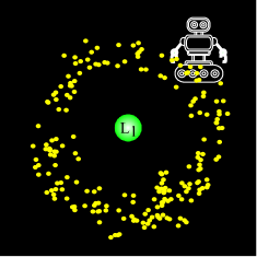
Like any other method, PF has its own advantages and disadvantages. Following a sample-based approach, PF is capable of representing any state distribution with arbitrary shape. To make this point clear, consider the localization scenarios of a mobile robot as shown in figure 11. In figure 11a, the robot can only sense its distance to landmark $L_{1}$. Without having access to the landmark angle with respect to the robot, after PF update step, the particles will be spread around the landmark forming a circular shape. Adding a second landmark $L_{2}$ to the scenario restricts the possible region for robot position leading to a bimodal distribution of the particles (figure 11b).

Using PF, process and measurement models are no longer required to be linear which has made PF very popular in the robotics community. The disadvantage of using samples-based representation is that the target distribution will not be captured with reasonable accuracy if the number of particles is not sufficient. On the other hand, as the number of particles is increased, so will the computational complexity. PF performance may degrade due to loss of diversity of particle samples. Methods like resample-move algorithm (Gilks and Berzuini, 2001), regularization (Musso et al., 2001), Rao-Blackwellisation (Liu and Chen, 1998), and multiple Monte-Carlo (Liu and Chen, 1998) can be utilized to deal with particles loss of diversity issue. PF has seen multiple variants such as sampling importance resampling (SIR) (Arulampalam et al., 2002), auxiliary sampling importance resampling (ASIR) (Pitt and Shephard, 1999), and regularized particle filter (RPF) (Doucet et al., 2001).

(a)

(b)

Figure 11. Illustration of particles distribution with (a) one landmark $L_{1}$, (b) two landmarks $\{L_{1},L_{2}\}$.

8. Obstacle avoidance

As mobile robots navigate through their operational environment, they have to deal with variety of obstacles in order to reach their destination. Therefore, the ability to avoid obstacles during navigation is a crucial module in autonomous systems. The location of obstacles may be known as part of the environment map but oftentimes the map is not known beforehand. Thus, it is highly desirable for autonomous mobile robots to be able to detect and avoid obstacles in real-time during navigation. Several obstacle avoidance methods exist in the literature which are reviewed in this section.

8.1. Legacy methods

The history of obstacle avoidance methods is almost as old as the emergence of mobile robots which is not surprising because without obstacle avoidance, mobility is not of much use. In this subsection, the classic methods of obstacle avoidance are reviewed.

8.1.1. Family of Bug algorithms

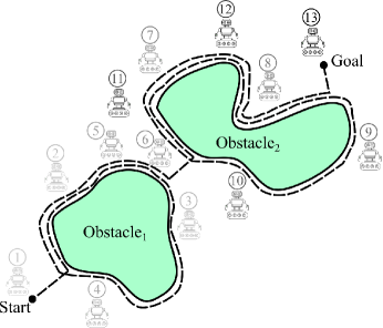
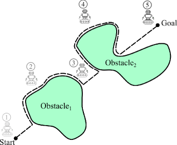
One of the simplest sets of obstacle avoidance methods is the family of Bug algorithms. As the name implies, these algorithms mimic the behavior of bugs upon encountering an obstacle on their way. The family of Bug algorithms began with the proposal of Bug1 and Bug2 (Lumelsky and Stepanov, 1986). The obstacle avoidance mechanisms of Bug1 and Bug2 have been depicted in figure 12a and 12b. According to figure 12a, whenever Bug1 bumps into an obstacle, it completes a cycle around it and in the second cycle, departs from the obstacle and continues its path toward the goal until the goal is reached or a new obstacle is detected. As shown in figure 12b, Bug2 assumes a hypothetical line from the start point to the goal point and circumvents any obstacle that intersects this line. Clearly, Bug2 is more efficient in terms of traveled distance compared to Bug1. Bug2+ (Antich et al., 2009b) is an improved version of Bug2. In Bug2+ the condition for switching from obstacle-boundary-following to motion-to-goal has been revised in order to reduce the length of the path traveled from the start to the goal.

Another algorithm from the Bug family is called CBUG (Gabriely and Rimon, 2008) which considers an ellipse with area equal to $A_{0}$ such that the start and the goal points form the ellipse’s focus points. Within this ellipse, Bug1 is executed in an attempt to reach the goal. If the goal is not reachable in the current ellipse, its area is increasd to $2^{i}A_{0}$ where $i$ is the iteration count. Within the new ellipse Bug1 is executed again. This trend is repeated until the goal is reached or it is concluded that the goal is not reachable. As shown in (Gabriely and Rimon, 2008), CBUG is an optimal online planner with constant memory requirement.

Bug2+ was originally designed to work with unknown environments but it has been combined with A* to exploit the map of the environment in order to reduce the length of the path to be traveled. The resulting method is an anytime planner called ABUG (Antich et al., 2009a). The advantage of anytime planners is that they plan a sub-optimal path quickly and revise the path during the navigation. The term anytime planner means that the planning process can be interrupted at any time and a valid path is available. The more time is given to the planner the better the planned path will be. In the case of ABUG, whenever an obstacle is encountered, Bug2+ can circumvent it either from the its left or right side. Given the map of the environment, all of the obstacles on the path is known beforehand. That is where A* comes in. For each obstacle, a binary node is created corresponding to going around the left or right side of the obstacle. Set of the obstacle form a binary search tree. Running A* on the tree gives us the optimal path from the start to the goal.

Perhaps one of the most important Bug algorithms is TangetBug (Kamon et al., 1998) based on which other methods such as WedgeBug (Laubach and Burdick, 1999) and CautiousBug (Magid and Rivlin, 2004) have been proposed. WedgeBug uses stereo vision for obstacle detection and its energy consumption, computational complexity, and memory usage has been minimized to meet the limited resources of mars rovers. The name WedgeBug is due to the fact that this algorithm is capable of navigation using the limited ($30^{\circ}$ to $45^{\circ}$) wedge-shaped field-of-view of stereo vision. This algorithm inspects a portion of the environment and if necessary, rotates its stereo vision system to inspect regions in the vicinity of the already observed region. This way, the limited field-of-view is dealt with. WedgeBug has been further modified to give birth to RoverBug (Laubach and Burdick, 2000) used in Rock7 mars rover (Laubach and Burdick, 1999).

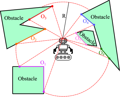
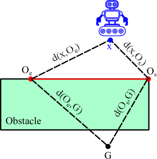
TangentBug utilizes range sensors such as laser scanners to detect obstacles before actually bumping into them. This way, the traveled path toward the goal is reduced significantly. Each detected obstacle is presented by its two endpoints. For example, in figure 12c, the robot is surrounded by four obstacles that have been represented by the set of six endpoints $\{O_{i},i=1,...,6\}$. TangentBug has two primary behavior modes namely motion-to-goal (M2G) and wall-following (WF). Initially, the behavior is set to M2G. In this mode, the robot takes the direct route toward goal $G$. In case an obstacle interferes with the direct route, the robot computes the heuristic distance for the two endpoints of the obstacle as depicted in figure 12d. The heuristic distance $H(.,.)$ is computed as

(25) $$H(x,G)=d(x,O_{*})+d(O_{*},G)$$

where $x$ is the robot current position, $O_{*}$ is one of the endpoints of the detected obstacle and $d(x,O_{*})$ is the Euclidean distance between robot position $x$ and endpoint $O_{*}$. After computing $H(x,G)$ for $O_{s}$ and $O_{e}$, the endpoint with minimum distance is chosen for bypassing the obstacle. M2G behavior is continued until the goal is reached or $d(x,G)$ starts to increase in which case the behavior is switched to WF. During WF, the robot follows the obstacle boundary until one of the conditions below is satisfied:

• The goal is reached $\rightarrow$ the algorithm halts with success.

• The robot completes a full cycle around the obstacle $\rightarrow$ the algorithm halts with failure since the goal is not reachable.

• The equation

  (26) $$d_{Reach}<d_{Followed}$$

  holds $\rightarrow$ the algorithm switches back to M2G behavior. $d_{Followed}$ is the distance between the goal $G$ and the point on the blocking obstacle boundary which is closest to $G$. Additionally, $d_{Reach}=d(v_{leave},G)$ where $v_{leave}$ is a node on the local tangent graph such that equation 26 holds.

(a)

(b)

(c)

(d)

Figure 12. Illustration of Bug algorithms: (a) Bug1 behavior, (b) Bug2 behavior, (c) local tangent graph used by TangentBug, (d) heuristic distance computation by TangentBug.

Another method that has been proposed with practical limitations in mind is I-Bug (Taylor and LaValle, 2009). This method has been designed to deal with inaccurate localization and noisy sensor readings. It is assumed that the goal point emits a signal which is detectable by a special sensor onboard the robot. As the robot gets closer to the goal, the signal strength increases and as it moves away from the goal, the signal strength drops. The signal strength measurement sensor is the only accurate sensor onboard the robot. In addition to this sensor, the robot is also equipped with a sensor that determines whether the robot is facing the goal or not. I-Bug is able to reach the goal although the robot does not know its position and obstacle positions in the environment. The family of Bug algorithm has even been extended for handling moving obstacles. The resulting algorith is called distance histogram Bug (DH-Bug) (Zhu et al., 2012).

8.1.2. Curvature velocity method

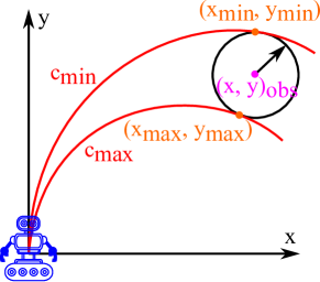
Bug algorithms are simple and easy to implement but they do not take into account the kinematics and/or dynamic constraints of the robot. On the contrary, curvature velocity method (CVM) (Simmons, 1996) considers the robot kinematics constraints and even dynamic constraints to some extent.

To perform obstacle avoidance, CVM transforms the physical constraints imposed by environment blocking obstacles as well as acceleration and speed limitations of the robot to the velocity space. Assuming that the robot only moves along circle arcs with curvature $c=\omega/v$, the velocity space consists of rotational ($\omega$) and translational velocity ($v$). CVM maps blocking obstacles from Cartesian grid to velocity space. The mapping is done based on the distance between the robot and the obstacles. After mapping, the range of $v$ and $\omega$ that must be filtered out due to the blocking obstacles can be determined.

Naturally, obstacle avoidance methods must be real-time. To satisfy this requirement, CVM models the obstacles with a circular shape (figure 13). Such modeling may lead to poor representation for the shape of some of the obstacles. This is the main drawback of CVM.

Figure 13. CVM computing valid curvatures for bypassing the blocking of the obstacle.

8.1.3. Potential field

Potential field (Khatib, 1986) was originally designed for control and obstacle avoidance of manipulator arms. However, due to its simplicity and effectiveness, potential field has been adopted by mobile robots community as well. Potential field models the robot as a point that is moved in the environment under influence of various attractive and repulsive potential fields. The goal is the source of attraction while the obstacles act as repulsive forces. In this setup, the total force $F(q)$ applied to the robot is the sum of repulsive ($F_{rep}$) and attractive ($F_{att}$) forces (Khatib, 1986):

(27) $$F(q)=F_{att}(q)+F_{rep}(q).$$

The attractive and repulsive forces are computed by taking the gradient from the attractive and repulsive potential functions. Therefore, it is necessary to define these functions such that they are differentiable:

(28) $$U_{att}(q) =\frac{1}{2}k_{att}\rho_{goal}^{2}(q),$$

(29) $$U_{rep}(q) =\begin{cases}\frac{1}{2}k_{rep}\left(\frac{1}{\rho(q)}-\frac{1}{\rho_{0}}\right)^{2},\>if\>\rho(q)<\rho_{0}\\ 0,\>if\rho(q)\geq\rho_{0}\\ \end{cases}$$

In equation 28, the attractive potential field is defined where $k_{att}$ is the scaling factor and $\rho_{goal}(q)$ is the Euclidean distance between point $q$ and goal $q_{goal}$. Looking at equation 28, it is clear that as the robot gets closer to the goal, the strength of the attractive field is reduced. This way when the robot reaches the goal, it is stopped.

In equation 29, the repulsive potential field is defined where $k_{rep}$ is the scaling factor and $\rho(q)$ is the minimum distance between the robot and the obstacle the repulsive field of which is to be computed for the robot. Additionally, in equation 29, $\rho_{0}$ is a threshold value. If the robot distance to the obstacle is less than $\rho_{0}$, it is affected by the repulsive field of the obstacle and otherwise, the robot is not affected by the field. As $\rho(q)$ is in the denominator of equation 29, the more the robot gets close to an obstacle, the stronger the repulsive field of the obstacle gets.

8.1.4. Dynamic window approach

Similar to CVM, dynamic window approach (DWA) (Fox et al., 1997) takes into account robot kinematics. To this end, DWA searches in velocity space which consists of all possible pairs of values of linear and angular velocities $(v,\omega)$. Another similarity between DWA and CVM is the assumption that the robot movement is only limited to circular arcs expressed as $(v,\omega)$. DWA forms a dynamic window in the velocity space such that the current linear and angular velocities of the robot will be at the center of that window. The dimensions of the window are determined based on the acceleration capabilities of the robot and the control cycle time. The infeasible velocity tuples $(v,\omega)$ within the dynamic window are pruned. The selection criterion of the tuples is that by using them, the robot will be able to stop before colliding with obstacles. The remaining tuples after the pruning are called admissible tuples. An objective function is applied on admissible tuples to determine the final movement direction for avoiding the obstacles and reaching the goal. The objective function reads as (Fox et al., 1997):

(30) $$O=a.heading(v,\omega)+b.velocity(v,\omega)+c.dist(v,\omega)$$

where heading measures the progress made toward the goal, velocity encourages fast forward motion, and dist is the distance between the robot and the closes obstacle during navigation.

8.1.5. Vector field histogram

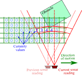
Virtual force field (VFF) (Borenstein and Koren, 1989) has been proposed to meet the obstacle avoidance requirements of relatively fast moving robots. VFF is capable of working with unknown environments having different configurations of obstacles using a ring of cheap sonar sensors around the robot chassis. VFF models the sensed obstacles as a 2D Cartesian histogram called certainty grid. The value in each cell of the grid represents the certainty (likelihood) that the cell is occupied with an obstacle. The grid is initialized with all zeros indicating that there are no cells occupied with obstacles.Each time a sonar reading is available, the certainty value of the appropriate histogram cell is incremented. The appropriate cell is determined based on the orientation of the sensor acoustic axis and measured range. During navigation, robot sonar readings are accumulated in the appropriate grid cells which leads to a reasonable estimation of the obstacle locations in the environment even though the sonar readings are not accurate. The process of accumulating sonar readings in the grid has been illustrated in figure 14a. As can be seen, the certainty values of the cells close to the obstacle have been increased due to successive sonar readings.

After populating the certainty grid with reasonable values, a rectangular sub-region of the grid (called active region) is considered with the robot at its center. The obstacles within the active region are considered for obstacle avoidance using the potential field (section 8.1.3) method.

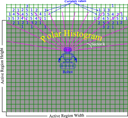
The main drawback of VFF is the inability to bypass certain obstacles configuration. For example, while moving down a hallway, the repulsive force exerted on the robot due to the left and right walls paralyzes VFF obstacle avoidance. The reason is the sudden reduction of the certainty grid to direction and magnitude of the repulsive force vector $F_{r}$ in a single step (Borenstein et al., 1991). This issue has been addressed by vector field histogram (VFH)(Borenstein et al., 1991) method using a two-step reduction procedure. After populating the certainty grid, it is reduced to a 1D polar histogram. To this end, the active region (the gray region in figure 14b) is partitioned into multiple sectors with angle $\alpha$. To compute the obstacle density for each sector $k$, for each certainty grid cell $\left(i,j\right)$, an obstacle vector with magnitude $m_{i,j}$ and direction $\beta_{i,j}$ is computed (Borenstein et al., 1991):

(31) $$\beta_{i,j}=\tan^{-1}\left(\frac{y_{i}-y_{r}}{x_{i}-x_{r}}\right),$$

(32) $$m_{i,j}=\left(c_{i,j}^{*}\right)^{2}\left(a-bd_{i,j}\right),$$

where $\left(x_{i},y_{i}\right)$ is the coordinates of cell $\left(i,j\right)$ and $c_{i,j}$ is its certainty value, $\left(x_{r},y_{r}\right)$ is the robot current position, $a$ and $b$ are positive constants, and $d_{i,j}$ is the distance between cell $\left(i,j\right)$ and the robot position. Based on the direction component $\beta_{i,j}$, the sector $k$ within which cell $\left(i,j\right)$ resides is decided (Borenstein et al., 1991):

$$k=\lfloor\frac{\beta_{i,j}}{\alpha}\rfloor.$$

After determining the appropriate sector for all of the certainty cells, the obstacle density for each sector $k$ is computed (Borenstein et al., 1991):

(33) $$h_{k}=\sum_{i,j}m_{i,j}.$$

Using equation 33, the polar histogram is formed with horizontal axis showing $[0,2\pi]$ degrees and vertical axis showing the obstacle density values for sectors at different angles. To determine the safe portions of the active region for robot movement, a threshold is applied on the polar histogram vertical axis. Sectors with obstacle density below the threshold are considered safe. VFH has been further extended to VFH+(Ulrich and Borenstein, 1998) to improve robot safety during navigation.

(a)

(b)

Figure 14. (a) VFF certainty grid update process using successive sonar readings, (b) illustration of how certainty grid is mapped to polar histogram by VFH method.

8.2. Obstacle avoidance using RL and DL

Over the years, computers have evolved dramatically reducing the computational burden for mobile robot platforms. This has paved the road toward using more powerful methods like DL and reinforcement learning which have higher processing power requirements. In this subsection, the state-of-the-art obstacle avoidance methods are reviewed.

To be able to avoid environmental obstacles, the distance between the robot and the obstacle is required. LiDAR sensors provide high precision range data but they are costly. Much cheaper alternatives are stereo cameras that provide depth data via disparity map computed between the two cameras. However, acquiring correct range data depends on appropriate calibration of stereo cameras and the estimated range is limited to a few meters (which is much less than LiDAR). To avoid the calibration process, one can use monocular cameras at the cost of losing depth data. However, recent advancements in DL have made it possible to estimate depth using only a single camera. To this end, Wenzel et al. (Wenzel et al., 2021) utilized generative adversarial networks (GAN) (Goodfellow et al., 2014) to convert RGB images to their corresponding depth images. This approach not only makes depth estimation from a single camera possible but also bridges the gap between simulation and real-world applications. The depth estimation is made possible thanks to the powerful feature extraction of DL methods. Bridging the gap between simulation and real-world is realized due to the fact that GAN does not care about the source of RGB images and it can estimate the depth maps for simulated as well as real images. The authors trained deep reinforcement learning agents such as deep Q networks (DQN) (Mnih et al., 2015) and proximal policy optimization (PPO) (Schulman et al., 2017) to generate appropriate control commands for input depth images. History of utilizing RL for obstacle avoidance precedes the birth of the infamous DQN approach. As an example, instead of relying on a lookup table, Huang et al. (Huang et al., 2005) used a NN to estimate the Q function of a Q-learning agent.

In addition to RL, DL-based obstacle avoidance modules can be trained in supervised manner as well. Liu et al. (Liu et al., 2017) implemented indoor obstacle avoidance by feeding raw images to a DL model based on AlexNet(Krizhevsky et al., 2017) and using the model output as steering commands. Based on the input image, the robot is steered left, right and commanded to go straight. The training of the DL model has been done using data collected during robot motion controlled by a human operator. To facilitate the implementation, ROS has been used.

9. Navigation methods

Autonomous navigation methods are either map-based or mapless. In map-based approaches, the environment map is known before the navigation starts but it is not the case for mapless methods. Obviously having the environment map facilitates efficient path planning. However, in many scenarios, the environment map is not known beforehand which has led to the development of mapless navigation and simultaneous localization and mapping (SLAM) reviewed in section 10.

9.1. Map-based navigation

The quality of map-based navigation is directly affected by how the environment map is represented and how accurate it is. Map representations are either metric or topological. In metric maps, the location of detected obstacles, landmarks, robot, etc. are expressed with respect to a certain reference frame (Meyer and Filliat, 2003). A typical metric map corresponding to environment in figure 15a has been illustrated in figure 15b in the form of a 2D grid. As can be seen, in the grid map, the detected obstacles, robot position, etc. are represented with respect to some specific $XY$ reference frame. Each cell of this grid represents the probability of being occupied with an obstacle. Grid cells with darker black are more likely to be occupied by obstacles. Probabilistic occupancy grids can be implemented using multiple approaches. Bayesian occupancy grid (BOG) (Moravec and Elfes, 1985) relies on Baye’s rule to estimate the probability of being occupied for each cell of the grid map. BOG has been used in some of the mapping approaches (Elfes, 1989; Hornung et al., 2013). Other methods to implement occupancy grid are based on reflection map (Thrun, 2002) and expectation maximization (Thrun, 2001).

(a)

(b)

(c)

Figure 15. Types of map representation: (a) actual environment, (b) metric map, (c) topological map.

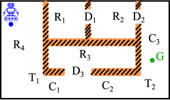
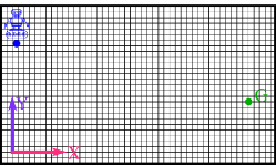
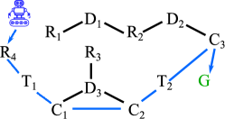
Naturally, when range sensors are available, expressing the environment map as a 2D or 3D grid is useful (Triebel et al., 2006; Hahnel et al., 2003; Grisetti et al., 2007). However, the memory requirement for storing map of large scale environments may be prohibitive(Fisher et al., 2021) since the memory size needed to store the map increases as range data are obtained and processed (Fisher et al., 2021). Several attempts have been made to keep the memory requirement of grid maps manageable (Hornung et al., 2013; Khan et al., 2014; Einhorn et al., 2010).

Apart from range sensors, camera sensors provide rich visual features as well. These features can be used to implement landmark maps (Smith et al., 1990; Montemerlo et al., 2002) which are effective for scenarios that locally distinguishable features are present in the environment. As an example, consider the environment in figure 15a again and assume that there are distinguishable features in different regions of this environment. Using these features, it is possible to generate a topological map similar to the one in figure 15c. Each node of the topological map represents a particular region in the environment based on the aforementioned distinguishable visual features. The regions that are accessible from one another are connected by edges in the topological map. For example $R_{4}$ (room 4) is accessible via $T_{1}$ (turn 1) which is shown in the topological map (15c) with an edge connecting $R_{4}$ to $T_{1}$. Treating the topological map as an undirected graph, off-the-shelf graph path planning algorithms can be used to find the shortest path between robot position and the goal position (denoted by $G$ in figure 15c). In real-world applications, it is likely that the environment map is only partially known. To carry out autonomous navigation under such circumstances, Sgorbissa and Renato proposed a hybrid navigation approach to exploit a possibly incomplete map of the environemnt and local perceptions during robot motion in order to achieve safe and collision-free navigation (Sgorbissa and Zaccaria, 2012).

9.2. Mapless

Autonomous mapless navigation is the act of controlling a mobile robot toward the desired destination without having access to the environment map. The problem of mapless navigation has been tackled several times. As pointed out in (Güzel, 2013), mapless vision-based techniques for indoor robot navigation can be categorized as:

• methods based on optical flow: in a nutshell, the motion of visual features in an image sequence is defined as optical flow. One of the mapless navigation methods based on optical flow is robee (Bernardino and Santos-Victor, 1998). In this method, vision system of a bee is mimicked using stereo cameras to navigate through the environment without colliding with obstacles. Optical flow has also been used to implement corridor following behavior (Duchon et al., 1998) as well as a feature-based navigation system (Temizer, 2001).

• appearance-based matching: in this approach, certain templates and images of the environment are memorized. The memorized data are then associated with controlling commands to guide the robot toward desired destination (DeSouza and Kak, 2002). The main challenge of appearance-based methods is finding appropriate methods to express environment in terms of prominent features as well as defining matching criteria for recognizing certain regions of the environment (Bonin-Font et al., 2008). Visual memory (Gaussier et al., 1997) is one of the appearance-based methods in which a sequence of images are captured during robot motion. The captured images are associated with appropriate motions required for reaching a specific destination. The images, their associated motions and a template matching algorithm can be used to construct the robot route. Another appearance-based approach is multidimensional histograms that are extracted based on statistical analysis (related to color, texture, and edge density) of captured images (Schiele and Crowley, 1996; Zhou et al., 2003). The recognition of places is done via matching histograms of stored places and histograms computed for the current position of the robot.

• object recognition: appearance-based approaches are primarily focused on memorizing their surrounding environment. However, symbolic navigation can be used instead (Kim and Nevatia, 1998, 1999). In this approach, the detected obstacle are stored in a 2D grid map called the S-map. Using this map, path planning is done and robot is given symbolic commands such as ”go to the main exit” or ”go to the corner in front of you” (Güzel, 2013)

• feature-based navigation methods: in these methods, the motion of the robot is determined by extracting features from image sequence and tracking the relative displacement of those features during robot movement. An example of feature-based navigation methods is funnel lane (Chen and Birchfield, 2009) in which a robot is tasked to follow a previously traversed path by matching image feed from its mono camera with the previously recorded image sequence called visual path. Funnel lane method is fully qualitative and does not need environment map of any kind. This method has been extended to sloped funnel lanes (Kassir et al., 2020) to address issues such as ambiguity between translation and rotation in certain scenarios and achieve better maneuverability.

RL has also been utilized to implement map-less autonomous navigation in highly dynamic environments where quick and adaptive action selection is required. As an example, Fan et al. (Fan et al., 2018) optimized a mapless navigation policy capable of robot control in highly dynamic environments such as pedestrian crowds. The optimization of the policy as a local planner was done using PPO and the policy was expressed as a CNN with four hidden layers.

10. SLAM

Simultaneous Localization And Mapping (SLAM) can be thought as a concept rather than a specific algorithm (Riisgaard and Blas, 2003). The term was coined after the original work of Hugh Durrant-Whyte and John J. Leonard (Leonard and Durrant-Whyte, 1991) whose research was founded based on earlier work by Smith, Self and Cheeseman (Smith et al., 1990). In a nutshell, SLAM objective is to localize a mobile robot in an unknown environment and at the same time estimate the environment map in terms of observed environment landmarks. Roughly speaking, the main components of SLAM are landmark extraction, data association, state estimation, and state and landmark update.

The high level steps of robot pose prediction and correction during SLAM have been depicted in figure 16. As shown in figure 16a, the robot measures its distance to three landmarks ($L_{1},L_{2},L_{3}$) and then moves to a new location. Using robot odometry model, the new location is predicted which has been shown as a robot figure with solid lines in figure 16b. Once again, the distance to the three landmarks is checked (figure 16c). Based on the obtained measurements, the robot pose is corrected leading to orange robot in figure 16d. As can be seen, the corrected pose is much closer to the ground truth pose (cyan robot in figure 16d). Sensors like IMU provide valuable information about the robot motion and play vital role in the prediction step of the SLAM (Karam et al., 2019). On the other hand, measured range data or visual features obtained from cameras are used in the update step of the SLAM in order to reduce the prediction error (Mohamed et al., 2019).

(a)

(b)

(c)

(d)

Figure 16. Illustration of mobile robot localization using SLAM and detected landmarks: (a) distance measurement to three landmarks $\{L_{1},L_{2},L_{3}\}$, (b) robot pose prediction after movement (dotted robot: old pose, solid robot: new predicted pose), (c) sensing landmarks again, (d) pose correction based on measurements in part c (white robot: predicted pose before correction, orange robot: pose after correction, cyan robot: true pose).

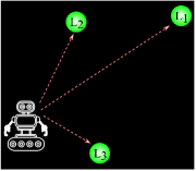
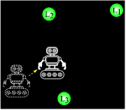
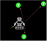
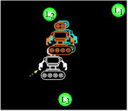
SLAM solutions can be categorized into two broad classes of filtering (online SLAM) and smoothing (full SLAM) methods (Alsadik and Karam, 2021) which are briefly introduced below.

Smoothing approaches rely on least-square optimization to estimate the robot full trajectory using all of the sensor measurements collected so far. Therefore, the memory consumption is high however, it is still possible to implement full SLAM in real-time (Strasdat et al., 2010). Estimatating the robot full trajectory $\hat{x}_{1:K}=\{\hat{x}_{k},k=1,...,K\}$ (with length $K$) given the sequence of control data $u_{1:K}=\{u_{k},k=1,...,K\}$ obtained from odometry sensors and observations $z_{1:K}=\{z_{k},k=1,...,K\}$ obtained from the environment is what separates full SLAM from online SLAM (Korkmaz et al., 2016). In full SLAM, the following posterior probability must be estimated (Grisetti et al., 2010):

(34) $$p(\hat{x}_{1:K}|u_{1:K},z_{1:K},x_{0})$$

where $x_{0}$ is the initial state of the robot at the start of the navigation. To estimate the posterior probability in equation (34), one has to deal with intractable high dimensional state spaces unless certain conditions such as static world and Markov property are assumed. Taking these two assumptions into account, Graph SLAM was proposed by Lu and Millios (Lu and Milios, 1997) which uses a graph-based representation to capture the underlying structure of the SLAM problem. Each graph node consists of a robot poseThe graph edges represent spatial constraints between nodes which are based on the collected observations $z_{k}$ or odometry data $u_{k}$.

Graph SLAM decomposes the problem into two parts: (a) graph construction (known as front-end) based on raw measurements and (b) finding the most likely configuration of the robot poses (known as back-end) such that the set of constraints imposed by the graph edges is satisfied (Grisetti et al., 2010). A typical pose-graph has been depicted in figure 17a in which $\Omega_{ij}$ is the information matrix and $e_{ij}=z_{ij}-\hat{z}(x_{i},x_{j})$ (the error function) is the difference between actual observation $z_{ij}$ gathered by the robot and the predicted observation $\hat{z}_{ij}(x_{i},x_{j})$ which represents $x_{j}$ in the coordinate frame of $x_{i}$. For more clarity, the connection between the two poses $x_{i}$ and $x_{j}$ due to their mutual observation $z_{ij}$ has been depicted in figure 17b. As can be seen, the uncertainty of observing $z_{ij}$ is captured by $\Omega_{ij}$.

In SLAM, data association is the matching of measurements obtained from the environment with the existing map which is vital for successful SLAM implementation (Zhou et al., 2016). Data association is usually handled by the SLAM front-end. To achieve a consistent estimate of the prior over robot trajectory $p(\hat{x}_{1:K}|z_{1:K},u_{1:K})$, interleaving of the front-end and the back-end is crucial. The data association problem has been tackled using different approaches based on joint compatibility branch and bound (Neira and Tardos, 2001), spectral clustering (Teller et al., 2006), and backtracking (Hähnel et al., 2005).

The second category of SLAM methods is online approaches which have lower memory consumption compared to full SLAM methods. This stems from the fact that online methods only rely on the previous pose estimate and sensor readings. However, lower memory consumption comes at the cost of decreased accuracy compared to the full SLAM approaches.

Apart from being online or full, SLAM methods can be also categorized based on the sensor(s) they use for collecting observations from the environment. Methods that use range sensors as their source of observation and methods that use camera sensors are called LiDAR SLAM and visual SLAM, respectively. Sections 10.1 and 10.2 are devoted to reviewing some of well-known methods belonging to LiDAR and visual SLAM and they are summarized in table 3.

(a)

(b)

Figure 17. (a) a typical pose-graph representation for Graph SLAM: nodes represent robot pose and edges express spatial constraint between nodes due to obtained measurements, (b) nodes $x_{i}$ and $x_{j}$ connection due to mutual observation $z_{ij}$.

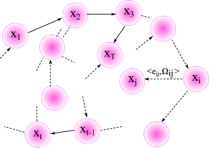
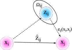
10.1. LiDAR SLAM

Indoor environments are heavily structured and having obstacles within 60 meters from the robot is quite likely. Such conditions are ideal for using laser scanners to sense and map the environment. SLAM approaches based on LiDAR sensors are known as LiDAR SLAM. Despite the ability to provide high precision data, LiDAR sensors are usually accompanied by hefty price tags making LiDAR SLAM an expensive solution.

The SLAM literature consists of various LiDAR-based SLAM approaches such as Hector slam (Kohlbrecher et al., 2013), keyframe-based 3D LiDAR SLAM (Guo et al., 2022), Google Cartographer (Hess et al., 2016), GMapping (Grisetti et al., 2007), and TinySLAM (Steux and El Hamzaoui, 2010). Traditionally, LiDAR sensors used rotary mechanisms to scan the surrounding environments. However, recent developments have led to low power and low cost LiDAR sensors based on Micro-Electro-Mechanical Systems MEMS technology. MEMS LiDARs are available at much more affordable prices which makes them ideal choices for the robotic researchers. However, lower cost of MEMS LiDAR comes at the price of shorter range (about nine meters) and smaller field of view (FOV) which makes LiDAR SLAM challenging. Fusing MEMS LiDAR data with other data sources such as IMU can improve the SLAM performance (Vonk, 2022). It has been shown that utilizing fast point cloud registration can further improve the localization and mapping quality (Wang et al., 2022). While using LiDAR sensors provide range data with outstanding accuracy, their relatively costly price tag is the motivation for using cheaper alternatives such as ultrasonic sensors (Cotugno et al., 2013; D’Alfonso et al., 2013; Jung et al., 2009; Yang, 2012).

10.2. Visual SLAM

Another type of SLAM methods is visual SLAM which is primarily focused on mono/stereo camera(s). Visual SLAM must not be confused with visual odometry (VO) (Yousif et al., 2015). Visual SLAM is all about preparing the global map of the explored environment whereas VO is used to estimate the robot pose locally.

One natural approach to implement visual SLAM is extracting features from camera images and use them to determine the scene geometry and camera pose. Feature-based methods are either based on filtering like the EKF-based visual-inertial odometry (Li and Mourikis, 2013) or based on keyframes (Klein and Murray, 2007a). At first glance, feature-based approaches seem very intuitive. However, these methods are limited to the information that are captured by the type of the features extracted. As pointed out in (Engel et al., 2014), feature-based methods will have difficulty with man-made environments. Some edge-based (Klein and Murray, 2008; Eade and Drummond, 2009) and region-based (Concha and Civera, 2014) have been proposed to tackle the aforementioned limitation. Among feature-based methods, Parallel Tracking And Mapping (PTAM) (Klein and Murray, 2007b, 2008, 2009) computational complexity is low enough to be runnable on a mobile phone using its camera as the source of visual data. PTAM uses FAST-10 corner detector (Rosten and Drummond, 2006) for feature extraction. ORB-SLAM (Mur-Artal et al., 2015) is based on ORB features (Rublee et al., 2011) capable of handling small/large and indoor/outdoor environments. The use of ORB features has made ORB-SLAM runnable in real-time without requiring a graphical processing unit (GPU). ORB-SLAM has received two important extensions resulting in second (Mur-Artal and Tardós, 2017a) and third (Campos et al., 2021) versions of this method. The second version provides support for stereo and RGBD cameras. The first version was limited to pin-hole camera model but the third version (based on first and second versions and ORB-SLAM-VI (Mur-Artal and Tardós, 2017b)) works with any camera type assuming that the camera module is provided. OV²SLAM (Ferrera et al., 2021) also offers a feature-based approach which is accurate, robust, and real-time outperforming ORB-SLAM.

It is also possible to take a direct (feature-less) approach in which all of the information in the image intensities are used. Using the direct approach, loss of prominent information due to limited representation power of features is avoided altogether. One of the direct methods is Large-Scale Direct Monocular SLAM (LSD-SLAM) (Engel et al., 2014) capable of building large-scale and consistent environment 3D maps in real-time. Direct Sparse Mapping (DSM) (Zubizarreta et al., 2020) is based on photometric bundle adjustment (PBA) that introduces the idea of map reuse in direct methods. DSM showed the importance of mid-term data association.

While majority of SLAM methods are either visual or LiDAR-based, Multi-cue Direct SLAM (MD-SLAM) (Di Giammarino et al., 2022) is the only open source approach that supports LiDAR and RGBD sensors in a unified manner.

Table 3. Summary of some of well known SLAM methods.

Method	Sensor					SLAM approach		Loop closure detection
	Radar	LiDAR	Visual			Online	Full
			Mono	Stereo	RGBD
Hector SLAM (Kohlbrecher et al., 2013)		✓				✓
LSD-SLAM (Engel et al., 2014, 2015)			✓				✓	✓
ORB-SLAM (Mur-Artal et al., 2015)			✓				✓	✓
ORB-SLAM2 (Mur-Artal and Tardós, 2017a)			✓	✓	✓		✓	✓
ORB-SLAM3 (Campos et al., 2021)			✓	✓	✓		✓	✓
ORB-SLAM-VI (Mur-Artal and Tardós, 2017b)			✓	✓	✓		✓	✓
Mono-SLAM (Davison, 2003; Davison et al., 2004; Molton et al., 2004; Davison et al., 2007)			✓			✓
PTAM (Klein and Murray, 2007b, 2008, 2009)			✓				✓
DSM (Zubizarreta et al., 2020)			✓				✓
OV2SLAM (Ferrera et al., 2021)			✓	✓			✓	✓
RT-SLAM (Roussillon et al., 2011)			✓	✓		✓		✓
Google Cartographer (Hess et al., 2016)		✓					✓	✓
GMapping (Grisetti et al., 2007)		✓				✓		✓
TinySLAM (Steux and El Hamzaoui, 2010)		✓				✓		✓
RadarSLAM (Hong et al., 2022)	✓						✓	✓
MD-SLAM (Di Giammarino et al., 2022)		✓			✓		✓	✓

10.3. Loop closure techniques

An efficient SLAM module must be capable of recognizing previously visited places in order to reduce the localization and mapping error that has been accumulated during multiple time steps. Such capability is called loop closure detection. Traditionally, feature descriptors such as SIFT (Lowe, 2004) and SURF (Bay et al., 2006) were used to loop closure detection. However, these methods are computationally inefficient for real-time applications. Researchers have developed loop closure mechanisms (Stumm et al., 2016; Cummins and Newman, 2008; Garcia-Fidalgo and Ortiz, 2018) based on bag-of-words (BoWs) approach to remedy the high computational load of descriptors such as SIFT and SURF. Bag-of-words refers to a dictionary of visual features extracted from the environment and clustered to form the so-called words. Despite being fast, BoWs rely on fixed visual features that must be known beforehand. It comes as no surprise that BoWs will not perform well in unexplored environments. To make BoWs adaptable to new regions (not explored before), it may be created in an online step (Garcia-Fidalgo and Ortiz, 2018). However, the memory requirements of the online approach are high. Following the significant achievements of DL in various domains, it has been adopted by the robotics community (Naseer et al., 2015; Zhang et al., 2017; Shin and Ho, 2018; Qin et al., 2018). A notable example of reinforcing SLAM with DL is DXSLAM (Li et al., 2020; dxs, [n. d.]) which uses CNN to extract salient features for boosting SLAM performance.

10.4. Public SLAM datasets

Conducting research on SLAM methods requires access to multiple sensors and mobile robot platforms. Apart from the cost of preparing the aforementioned hardware, it may be difficult for individual researchers to put together a SLAM-capable hardware setup. An alternative approach is development and evaluation of SLAM methods on public datasets obtained from real robots. Yin and Berger (Yin and Berger, 2017) have reviewed 27 publicly available datasets that have been collected on public roads. Some of these datasets are suited for evaluation of SLAM approaches. The summary of these datasets is available in table 4. As can be seen, existing datasets cover variety of environments being indoor, and outdoor, having different weather and lighting conditions, etc. Recently, semantic SLAM has gained popularity which is the inspiration for preparing synthetic datasets suitable for semantic SLAM. SSS-dataset (ShanghaiTech Semantic SLAM) (Cao et al., 2020) is an example of such datasets which provides accurate ground truth for the scene composition and individual object shapes and poses.

Table 4. Summary of public SLAM datasets.

Dataset	Indoor	Urban	Suburb	Rural	Attributes	Loop closure	Sensor data
AMUSE (Koschorrek et al., 2013)		✓			Weather: {snowy, water & snow on lens}	✓	Omni-directional multi-camera, height sensor, IMU, velocity sensor, GPS
CCSAD (Guzmán et al., 2015)		✓			Recorded in developing countries, variable lighting, tunnel at night, narrow roads		Stereo camera, IMU, GPS
Cheddar Gorge (Simpson et al., 2011)				✓	Weather: {dry, sunny, clear, cold}	✓	Stereo/mono camera, mono IR camera, Velodyne 64 LiDAR, high-end GPS/IMU, low-end IMU, wheel encoders, laser tracker for sensor pose measurement
CMU Visual Localization Dataset (Badino et al., 2011)		✓	✓		Versatile weather & light conditions	✓	2 Mono cameras, 4 Sick LiDARs, GPS, IMU
ETH3D (Schops et al., 2019)	✓	✓			Suitable for evaluating visual inertial mono, stereo, and RGB-D-SLAM (eth, [n. d.]a), accompanying source code (eth, [n. d.]b), synchronized global shutter cameras, modeling rolling shutter effect not required	✓	Stereo/mono/RGBD cameras, IMU, Faro Focus X 330 laser scanner
Ford (Pandey et al., 2011)		✓			Weather condition: sunny, time-registered data, accompanied with utility source codes	✓	GPS, IMU, Velodyne 3D LiDAR, 2 push-broom forward looking Riegl LiDARs, omnidirectional camera
2D Cartographer Backpack Deutsches Museum (2DC, [n. d.])	✓				ROS .bag format, intended for 2D SLAM	✓	IMU, two 2D LiDAR (horizontal and vertical)
KITTI (Geiger et al., 2013)		✓		✓	grayscale/color images, ground truth provided based on GPS and laser scanner	✓	2 Mono grayscale cameras, 2 mono color cameras, Velodyne 64 LiDAR, GPS, IMU
Malaga (Blanco-Claraco et al., 2014)		✓	✓		Direct sun, accompanied with C++ sample codes for parsing raw log files	✓	Stereo camera, 3 Hokuyo UTM-30LX LiDAR, 2 Sick LiDARs, GPS, IMU
Oxford (Maddern et al., 2017)		✓			Different lighting/weather conditions, accompanied with Matlab, Python tools	✓	Stereo camera, 3 monocular color cameras, 2 Sick 2D LiDARs, Sick 3D LiDAR, GPS, INS

11. Future work

In this section, the future research direction for autonomous mobile robots is presented.

11.1. Mobile robots deployment in real-world

One of the ultimate goals of pursuing research on autonomous mobile robots is their deployment in manufacturing, hospitals, warehousing, etc. Implementing a multi-robot setup is quite natural to complete tasks faster(Nahavandi et al., 2022). Deciding on the operations that must be carried out in centralized or decentralized manner is an important future direction (Fragapane et al., 2021). It is also necessary to support multi-robot setup with efficient decision making about the set of tools that must be mounted on the robots to carry out specific tasks (Fragapane et al., 2021).

Autonomous navigation has also been used to develop autonomous ships with different levels of autonomy. As future works, it is important to establish cooperative behavior between maritime autonomous surface ships (MASS) which have autonomy levels of D3 and D4. D3 autonomy is remote control of ships without having seafarers onboard while D4 refers to fully autonomous ships (Organization, 2018). It is also critical to analyze safety in human-machine interaction setup (Kim et al., 2022).

11.2. SLAM

Although there is multitude of works in SLAM literature, due to complex and challenging nature of SLAM, there are still important research gaps for future work. For efficient SLAM implementation, it is crucial to keep balance between exploration (visiting new places) and exploitation (revisiting known places for uncertainty reduction) (Thrun, 1995) which is addressed by active SLAM. Future works (Placed et al., 2022) for active SLAM consist of active spatial perception, proposing evaluation metrics to facilitate comparison of methods, and performing benchmarks to move toward real-world applications.

SLAM methods commonly assume that the world is static. However, real world is full of moving objects which contribute to failure of feature recognition causing tracking failure in SLAM (Deng et al., 2018). As future work, DL and spectral methods (Xu et al., 2021; Xu et al., 2019) can be used to achieve more robust feature recognition and tracking (Macario Barros et al., 2022). It may be possible to detect and exclude dynamic objects from map construction process of SLAM. Currently, dynamic SLAM methods such as (Sun et al., 2017, 2018) exist to deal with dynamicity of the environment. Using semantic information to devise semantic SLAM is an ongoing field of research for addressing dynamic SLAM (Macario Barros et al., 2022). Additionally, using semantic SLAM to take the autonomy level of robots to the next level is challenging future task (Chen et al., 2022b).

While DL has shown some merits for loop closure detection, due to its limitations, the true loop detection is still unaddressed (Arshad and Kim, 2021). The limitation is due to sensitivity of vision-based loop closure detection methods to different illumination conditions. LiDAR-based loop does not suffer from such limitations however its performance is degraded due to weather conditions such as rain. Coming up with hybrid methods, exploiting the strengths and covering the weaknesses of both LiDAR-based and DL-based methods seems to be a necessary future direction (Arshad and Kim, 2021).

To deploy visual SLAM methods in real world applications, they must be executable on embedded platforms such as smartphones which have limited processing power. Therefore, one of the important future works for SLAM is to keep the balance between real-time execution and accuracy (Chen et al., 2022b).

11.3. Autonomous exploration in unseen environment

Being able to navigate and explore unseen environments autonomously is highly desirable. To this end, Shah et al. exploited RL to propose a method called RECON (Rapid Exploration Controllers for Outcome-driven Navigation) (Shah et al., 2021) which was trained on visual dataset (rec, [n. d.]) collected during 18 months from diverse real-world environments including different seasons and lighting conditions. Two primary components of RECON are uncertainty-aware and context conditioned goal representation as well as topological map representation. Nodes of the map represent egocentric observations and the edges are distances between nodes.

Extending RECON, Shah and Levine (Shah and Levine, 2022) focused on long-range autonomous navigation through unseen outdoor environments without requiring accurate map and/or sensor data. The advantage of their method called ViKiNG (Vision-Based Kilometer-Scale Navigation with Geographic Hints) is twofold. First, ViKiNG manages to reach the given destination using inaccurate data (GPS coordinates, satellite maps and schematic roadmaps ) as a heuristic during planning. Second, this method does not build geometric maps and only relies on topological representation of the environment. This way, the issue of building and storing environment dense map for long distances is not encountered on robots with lightweight processing/storage platforms. The authors have trained ViKiNG using trajectories that are only 80 meters long but have managed to reach goals up to three kilometers away. As pointed out by Shah and Levine, one of the important future works is devising models similar to ViKiNG that are capable of accepting inputs such as textual instructions and paper maps.

12. Conclusion

Autonomous navigation has come a long way but the journey still continues. Different sensor combinations and mathematical approaches have been tried leading to variety of approaches; each having advantages and disadvantages of their own. In this paper, we strove to present a comprehensive review on different aspects of autonomous mobile robots including localization methods, obstacle avoidance, sensor types, SLAM, etc. We also tried to highlight the role of DL in reinforcing obstacle avoidance and SLAM approaches. The common simulation tools and their properties were reviewed. Additionally, publicly available datasets (containing real sensor data) for implementing SLAM without having an actual robot were introduced. Finally, the possible directions for future research were pointed out.