An Lpsuperscript𝐿𝑝L^{p}-primal-dual finite element method for first-order transport problems

Dan Li School of Mathematical Sciences, Nanjing Normal University, Nanjing 210023, China (danlimath@163.com).    Chunmei Wang Department of Mathematics, University of Florida, Gainesville, FL 32611 (chunmei.wang@ufl.edu). The research of Chunmei Wang was partially supported by National Science Foundation Grants DMS-2136380 and DMS-2206332.    Junping Wang Division of Mathematical Sciences, National Science Foundation, Alexandria, VA 22314 (jwang@nsf.gov). The research of Junping Wang was supported by the NSF IR/D program, while working at National Science Foundation. However, any opinion, finding, and conclusions or recommendations expressed in this material are those of the author and do not necessarily reflect the views of the National Science Foundation.
Abstract

A new Lpsuperscript𝐿𝑝L^{p}-primal-dual weak Galerkin method (Lpsuperscript𝐿𝑝L^{p}-PDWG) with p>1𝑝1p>1 is proposed for the first-order transport problems. The existence and uniqueness of the Lpsuperscript𝐿𝑝L^{p}-PDWG numerical solutions is established. In addition, the Lpsuperscript𝐿𝑝L^{p}-PDWG method offers a numerical solution which retains mass conservation locally on each element. An optimal order error estimate is established for the primal variable. A series of numerical results are presented to verify the efficiency and accuracy of the proposed Lpsuperscript𝐿𝑝L^{p}-PDWG scheme.

keywords:
primal-dual, weak Galerkin, transport equation, weak regularity, Lpsuperscript𝐿𝑝L^{p} stabilizer, conservative methods.
AMS:
Primary, 65N30, 65N15, 65N12; Secondary, 35L02, 35F15, 35B45.

1 Introduction

This paper is concerned with the new development of numerical methods for the first-order linear convection equations in divergence form by using a new Lpsuperscript𝐿𝑝L^{p}-primal-dual weak Galerkin method. For simplicity, we consider the model problem that seeks an unknown function u𝑒u satisfying

(1.1) βˆ‡β‹…(πœ·β€‹u)+c​u=f,in ​Ω,u=g,onΒ β€‹Ξ“βˆ’,\begin{split}\nabla\cdot({\boldsymbol{\beta}}u)+cu=&f,\qquad\text{in }\Omega,\\ u=&g,\qquad\text{on }\Gamma_{-},\end{split}

where Ξ©βŠ‚β„d​(d=2,3)Ξ©superscriptℝ𝑑𝑑23\Omega\subset\mathbb{R}^{d}(d=2,3) is an open bounded and connected domain with Lipschitz continuous boundary βˆ‚Ξ©Ξ©\partial\Omega, Ξ“βˆ’subscriptΞ“\Gamma_{-} is the inflow portion of the boundary such that

Ξ“βˆ’={π±βˆˆβˆ‚Ξ©:πœ·β€‹(𝐱)⋅𝐧<0},subscriptΞ“conditional-setπ±Ξ©β‹…πœ·π±π§0\Gamma_{-}=\{{\mathbf{x}}\in\partial\Omega:\ {\boldsymbol{\beta}}({\mathbf{x}})\cdot{\mathbf{n}}<0\},

with 𝐧𝐧{\mathbf{n}} being an unit outward normal vector along the boundary βˆ‚Ξ©Ξ©\partial\Omega. Assume that the convection vector 𝜷∈[Lβˆžβ€‹(Ξ©)]d𝜷superscriptdelimited-[]superscript𝐿Ω𝑑{\boldsymbol{\beta}}\in[L^{\infty}(\Omega)]^{d} is locally W1,∞superscriptπ‘Š1W^{1,\infty}, the reaction coefficient c∈Lβˆžβ€‹(Ξ©)𝑐superscript𝐿Ωc\in L^{\infty}(\Omega) is bounded, the load function f∈Lq​(Ξ©)𝑓superscriptπΏπ‘žΞ©f\in L^{q}(\Omega) and the inflow boundary data g∈Lq​(Ξ“βˆ’)𝑔superscriptπΏπ‘žsubscriptΞ“g\in L^{q}(\Gamma_{-}) are two given functions with 1p+1q=11𝑝1π‘ž1\frac{1}{p}+\frac{1}{q}=1.

The first-order linear convection equations have wide applications in science and engineering problems. For the non-smooth inflow boundary data, the exact solution of model problem (1.1) possesses discontinuity. It is well known that the solution discontinuity imposes a challenge on the development of efficient numerical methods. To address the challenge, a variety of numerical methods for linear convection equations have been developed such as streamline-upwind Petrov-Galerkin method [1, 20], stabilized finite element methods [2, 18, 17, 3, 8], least-square finite element method [23, 10, 9, 25], and discontinuous Galerkin finite element methods [21, 19, 11, 12, 4, 24, 5, 6, 7]. Most of the aforementioned numerical methods assumed the coercivity assumption in the form of c+12β€‹βˆ‡β‹…πœ·β‰₯Ξ±0>0𝑐⋅12βˆ‡πœ·subscript𝛼00c+\frac{1}{2}\nabla\cdot{\boldsymbol{\beta}}\geq\alpha_{0}>0 for a fixed constant Ξ±0subscript𝛼0\alpha_{0} or alike. However, this assumption imposes a strong restriction in practice and often rules out some important physics such as exothermic reactions [2]. In [2], the authors developed a stabilized finite element method for linear transport equation with smooth coefficients 𝜷∈[W2,βˆžβ€‹(Ξ©)]d𝜷superscriptdelimited-[]superscriptπ‘Š2Ω𝑑{\boldsymbol{\beta}}\in[W^{2,\infty}(\Omega)]^{d} and c∈W1,βˆžβ€‹(Ξ©)𝑐superscriptπ‘Š1Ξ©c\in W^{1,\infty}(\Omega). In [27], the primal-dual weak Galerkin method was proposed and analyzed for the linear transport equation with 𝜷∈[W1,βˆžβ€‹(Ξ©)]d𝜷superscriptdelimited-[]superscriptπ‘Š1Ω𝑑{\boldsymbol{\beta}}\in[W^{1,\infty}(\Omega)]^{d} and c∈Lβˆžβ€‹(Ξ©)𝑐superscript𝐿Ωc\in L^{\infty}(\Omega). In [22], the authors proposed a new primal-dual weak Galerkin method for transport equation in non-divergence form with locally coefficients 𝜷∈[C1,Ξ±0]d𝜷superscriptdelimited-[]superscript𝐢1subscript𝛼0𝑑{\boldsymbol{\beta}}\in[C^{1,\alpha_{0}}]^{d} and c∈C0,Ξ±0𝑐superscript𝐢0subscript𝛼0c\in C^{0,\alpha_{0}}, where the PDWG method was first developed in [28] to solve many partial differential equations [15, 31, 32, 33, 34, 35] that are difficult to be approximated by using traditional numerical methods. The basic principle of primal-dual weak Galerkin method is to characterize this method as a linear L2superscript𝐿2L^{2} minimization problem with constraints that satisfy the certain conditions weakly on each finite element.

The objective of this paper is to present an Lpsuperscript𝐿𝑝L^{p}-primal-dual weak Galerkin method for the linear convection problem (1.1) without enforcing the coercivity condition on the convection vector 𝜷𝜷{\boldsymbol{\beta}} and the reaction coefficient c𝑐c. The Lpsuperscript𝐿𝑝L^{p}-PDWG method has been successfully applied to solve some partial differential equations such as div-curl systems [16], second order elliptic equations in non-divergence form [14], convection-diffusion equations [13]. Our numerical algorithm can be characterized as a constrained nonlinear Lpsuperscript𝐿𝑝L^{p} optimization problem with constraints that satisfy the model equation weakly on each finite element by using locally designed weak gradient operator. Different from the numerical method in [27, 22], a more general Lpsuperscript𝐿𝑝L^{p} stabilizer is introduced. The solvability and stability of Lpsuperscript𝐿𝑝L^{p}-PDWG method is discussed by introducing an equivalent min-max characterization and an error estimate of optimal order is established for the numerical approximation. In addition, a mass conservative numerical scheme is constructed to approximate the linear convection problem (1.1) where this numerical scheme is based on the Lpsuperscript𝐿𝑝L^{p}-primal-dual weak Galerkin technique.

This paper is organized as follows. In Section 2, we introduce a weak formulation for the first-order transport problem (1.1) and then briefly review the definition of weak gradient operator. Section 3 presents an Lpsuperscript𝐿𝑝L^{p}-PDWG scheme for the model problem (1.1). The goal of Section 4 is to study the solution existence and uniqueness for this numerical scheme. Section 5 is devoted to discussing the mass conservation property locally on each polytopal element. Section 6 derives an error equation and some error estimates for the numerical approximation are established in Section 7. In Section 8, various numerical experiments are presented to demonstrate the performance of the Lpsuperscript𝐿𝑝L^{p}-primal-dual weak Galerkin method.

This paper follows the standard definitions and notations for Sobolev spaces and norms. Let DβŠ‚β„d𝐷superscriptℝ𝑑D\subset\mathbb{R}^{d} be any open bounded domain with Lipschitz continuous boundary. Denote by βˆ₯β‹…βˆ₯Lp​(D)\|\cdot\|_{L^{p}(D)} the norm in the Sobolev space W0,p​(D)superscriptπ‘Š0𝑝𝐷W^{0,p}(D). Moreover, we use C𝐢C to denote the generic positive constant independent of meshsize or functions appearing in the equalities.

2 Weak Formulation and Discrete Weak Gradient

In this section, we shall introduce the weak formulation for the linear convection equation in divergence form (1.1). In addition, we shall briefly review the weak gradient operator as well as its discrete version [29].

The weak formulation for the model problem (1.1) is as follows: Find u∈Lq​(Ξ©)𝑒superscriptπΏπ‘žΞ©u\in L^{q}(\Omega) such that

(2.1) (u,πœ·β‹…βˆ‡Οƒβˆ’c​σ)=⟨g,πœ·β‹…π§β€‹ΟƒβŸ©Ξ“βˆ’βˆ’(f,Οƒ),βˆ€ΟƒβˆˆW0,Ξ“+1,p​(Ξ©).formulae-sequenceπ‘’β‹…πœ·βˆ‡πœŽπ‘πœŽsubscriptπ‘”β‹…πœ·π§πœŽsubscriptΞ“π‘“πœŽfor-all𝜎superscriptsubscriptπ‘Š0subscriptΞ“1𝑝Ω(u,{\boldsymbol{\beta}}\cdot\nabla\sigma-c\sigma)=\langle g,{\boldsymbol{\beta}}\cdot{\mathbf{n}}\sigma\rangle_{\Gamma_{-}}-(f,\sigma),\qquad\forall\sigma\in W_{0,\Gamma_{+}}^{1,p}(\Omega).

Here Ξ“+=βˆ‚Ξ©βˆ–Ξ“βˆ’subscriptΓΩsubscriptΞ“\Gamma_{+}=\partial\Omega\setminus\Gamma_{-} is the outflow boundary satisfying πœ·β‹…π§β‰₯0β‹…πœ·π§0{\boldsymbol{\beta}}\cdot{\mathbf{n}}\geq 0, and W0,Ξ“+1,p​(Ξ©)superscriptsubscriptπ‘Š0subscriptΞ“1𝑝ΩW_{0,\Gamma_{+}}^{1,p}(\Omega) is the subspace of W1,p​(Ξ©)superscriptπ‘Š1𝑝ΩW^{1,p}(\Omega) with vanishing boundary value on Ξ“+subscriptΞ“\Gamma_{+}; i.e.,

W0,Ξ“+1,p​(Ξ©)={v∈W1,p​(Ξ©):v=0​on​Γ+}.superscriptsubscriptπ‘Š0subscriptΞ“1𝑝Ωconditional-set𝑣superscriptπ‘Š1𝑝Ω𝑣0onsubscriptΞ“W_{0,\Gamma_{+}}^{1,p}(\Omega)=\{v\in W^{1,p}(\Omega):v=0\ \text{on}\ \Gamma_{+}\}.

Let T𝑇T be a polygonal or polyhedral domain with boundary βˆ‚T𝑇\partial T. Denote by v={v0,vb}𝑣subscript𝑣0subscript𝑣𝑏v=\{v_{0},v_{b}\} a weak function on T𝑇T such that v0∈Lp​(T)subscript𝑣0superscript𝐿𝑝𝑇v_{0}\in L^{p}(T) and vb∈Lp​(βˆ‚T)subscript𝑣𝑏superscript𝐿𝑝𝑇v_{b}\in L^{p}(\partial T). The components v0subscript𝑣0v_{0} and vbsubscript𝑣𝑏v_{b} represent the values of v𝑣v in the interior and on the boundary of T𝑇T, respectively. Note that vbsubscript𝑣𝑏v_{b} may not necessarily be the trace of v0subscript𝑣0v_{0} on βˆ‚T𝑇\partial T. Denote by 𝒲​(T)𝒲𝑇{\mathcal{W}}(T) the space of weak functions on T𝑇T; i.e.,

𝒲​(T)={v={v0,vb}:v0∈Lp​(T),vb∈Lp​(βˆ‚T)}.𝒲𝑇conditional-set𝑣subscript𝑣0subscript𝑣𝑏formulae-sequencesubscript𝑣0superscript𝐿𝑝𝑇subscript𝑣𝑏superscript𝐿𝑝𝑇{\mathcal{W}}(T)=\{v=\{v_{0},v_{b}\}:v_{0}\in L^{p}(T),v_{b}\in L^{p}(\partial T)\}.

The weak gradient of vβˆˆπ’²β€‹(T)𝑣𝒲𝑇v\in{\mathcal{W}}(T), denoted by βˆ‡wvsubscriptβˆ‡π‘€π‘£\nabla_{w}v, is defined as a continuous linear functional in the Sobolev space [W1,q​(T)]dsuperscriptdelimited-[]superscriptπ‘Š1π‘žπ‘‡π‘‘[W^{1,q}(T)]^{d} satisfying

(βˆ‡wv,𝝍)T=βˆ’(v0,βˆ‡β‹…π)T+⟨vb,𝝍⋅nβŸ©βˆ‚T,βˆ€πβˆˆ[W1,q​(T)]d.formulae-sequencesubscriptsubscriptβˆ‡π‘€π‘£ππ‘‡subscriptsubscript𝑣0β‹…βˆ‡ππ‘‡subscriptsubscript𝑣𝑏⋅𝝍n𝑇for-all𝝍superscriptdelimited-[]superscriptπ‘Š1π‘žπ‘‡π‘‘(\nabla_{w}v,\boldsymbol{\psi})_{T}=-(v_{0},\nabla\cdot\boldsymbol{\psi})_{T}+\langle v_{b},\boldsymbol{\psi}\cdot\textbf{n}\rangle_{\partial T},\qquad\forall\boldsymbol{\psi}\in[W^{1,q}(T)]^{d}.

Denote by Pr​(T)subscriptπ‘ƒπ‘Ÿπ‘‡P_{r}(T) the space of polynomials on T𝑇T with degree no more than rπ‘Ÿr. A discrete version of βˆ‡wvsubscriptβˆ‡π‘€π‘£\nabla_{w}v for vβˆˆπ’²β€‹(T)𝑣𝒲𝑇v\in{\mathcal{W}}(T), denoted by βˆ‡w,r,Tvsubscriptβˆ‡π‘€π‘Ÿπ‘‡π‘£\nabla_{w,r,T}v, is defined as a unique polynomial vector in [Pr​(T)]dsuperscriptdelimited-[]subscriptπ‘ƒπ‘Ÿπ‘‡π‘‘[P_{r}(T)]^{d} such that

(2.2) (βˆ‡w,r,Tv,𝝍)T=βˆ’(v0,βˆ‡β‹…π)T+⟨vb,𝝍⋅nβŸ©βˆ‚T,βˆ€πβˆˆ[Pr​(T)]d,formulae-sequencesubscriptsubscriptβˆ‡π‘€π‘Ÿπ‘‡π‘£ππ‘‡subscriptsubscript𝑣0β‹…βˆ‡ππ‘‡subscriptsubscript𝑣𝑏⋅𝝍n𝑇for-all𝝍superscriptdelimited-[]subscriptπ‘ƒπ‘Ÿπ‘‡π‘‘(\nabla_{w,r,T}v,\boldsymbol{\psi})_{T}=-(v_{0},\nabla\cdot\boldsymbol{\psi})_{T}+\langle v_{b},\boldsymbol{\psi}\cdot\textbf{n}\rangle_{\partial T},\quad\forall\boldsymbol{\psi}\in[P_{r}(T)]^{d},

which, using the usual integration by parts, yields

(2.3) (βˆ‡w,r,Tv,𝝍)T=(βˆ‡v0,𝝍)Tβˆ’βŸ¨v0βˆ’vb,𝝍⋅nβŸ©βˆ‚T,βˆ€πβˆˆ[Pr​(T)]d,formulae-sequencesubscriptsubscriptβˆ‡π‘€π‘Ÿπ‘‡π‘£ππ‘‡subscriptβˆ‡subscript𝑣0𝝍𝑇subscriptsubscript𝑣0subscript𝑣𝑏⋅𝝍n𝑇for-all𝝍superscriptdelimited-[]subscriptπ‘ƒπ‘Ÿπ‘‡π‘‘(\nabla_{w,r,T}v,\boldsymbol{\psi})_{T}=(\nabla v_{0},\boldsymbol{\psi})_{T}-\langle v_{0}-v_{b},\boldsymbol{\psi}\cdot\textbf{n}\rangle_{\partial T},\quad\forall\boldsymbol{\psi}\in[P_{r}(T)]^{d},

provided that v0∈W1,p​(T)subscript𝑣0superscriptπ‘Š1𝑝𝑇v_{0}\in W^{1,p}(T).

3 Lpsuperscript𝐿𝑝L^{p} Primal-Dual Weak Galerkin Algorithm

Denote by 𝒯hsubscriptπ’―β„Ž{\cal T}_{h} a partition of the domain Ξ©βŠ‚β„d​(d=2,3)Ξ©superscriptℝ𝑑𝑑23\Omega\subset{\mathbb{R}}^{d}(d=2,3) into polygons in 2D or polyhedra in 3D which is shape regular described as in [30]. Let β„°hsubscriptβ„°β„Ž{\mathcal{E}}_{h} be the set of all edges or flat faces in 𝒯hsubscriptπ’―β„Ž{\cal T}_{h} and β„°h0=β„°hβˆ–βˆ‚Ξ©superscriptsubscriptβ„°β„Ž0subscriptβ„°β„ŽΞ©{\mathcal{E}}_{h}^{0}={\mathcal{E}}_{h}\setminus\partial\Omega be the set of all interior edges or flat faces. Denote by hTsubscriptβ„Žπ‘‡h_{T} the meshsize of Tβˆˆπ’―h𝑇subscriptπ’―β„ŽT\in{\cal T}_{h} and h=maxTβˆˆπ’―h⁑hTβ„Žsubscript𝑇subscriptπ’―β„Žsubscriptβ„Žπ‘‡h=\max_{T\in{\cal T}_{h}}h_{T} the meshsize of the partition 𝒯hsubscriptπ’―β„Ž{\cal T}_{h}.

For any integer jβ‰₯0𝑗0j\geq 0, let Wj​(T)subscriptπ‘Šπ‘—π‘‡W_{j}(T) be the local space of discrete weak functions; i.e.,

Wj​(T)={{Οƒ0,Οƒb}:Οƒ0∈Pj​(T),Οƒb∈Pj​(e),eβŠ‚βˆ‚T}.subscriptπ‘Šπ‘—π‘‡conditional-setsubscript𝜎0subscriptπœŽπ‘formulae-sequencesubscript𝜎0subscript𝑃𝑗𝑇formulae-sequencesubscriptπœŽπ‘subscript𝑃𝑗𝑒𝑒𝑇W_{j}(T)=\{\{\sigma_{0},\sigma_{b}\}:\sigma_{0}\in P_{j}(T),\sigma_{b}\in P_{j}(e),e\subset\partial T\}.

Patching Wj​(T)subscriptπ‘Šπ‘—π‘‡W_{j}(T) over all the elements Tβˆˆπ’―h𝑇subscriptπ’―β„ŽT\in{\cal T}_{h} through a common value vbsubscript𝑣𝑏v_{b} on the interior interface β„°h0superscriptsubscriptβ„°β„Ž0{\mathcal{E}}_{h}^{0} gives rise to a global weak finite element space Wj,hsubscriptπ‘Šπ‘—β„ŽW_{j,h}. Let Wj,h0,Ξ“+superscriptsubscriptπ‘Šπ‘—β„Ž0subscriptΞ“W_{j,h}^{0,\Gamma_{+}} be the subspace of Wj,hsubscriptπ‘Šπ‘—β„ŽW_{j,h} with vanishing boundary value on Ξ“+subscriptΞ“\Gamma_{+}; i.e.,

Wj,h0,Ξ“+={{Οƒ0,Οƒb}∈Wj,h:Οƒb|e=0,eβŠ‚Ξ“+}.superscriptsubscriptπ‘Šπ‘—β„Ž0subscriptΞ“conditional-setsubscript𝜎0subscriptπœŽπ‘subscriptπ‘Šπ‘—β„Žformulae-sequenceevaluated-atsubscriptπœŽπ‘π‘’0𝑒subscriptΞ“W_{j,h}^{0,\Gamma_{+}}=\{\{\sigma_{0},\sigma_{b}\}\in W_{j,h}:\sigma_{b}|_{e}=0,e\subset\Gamma_{+}\}.

For any integer kβ‰₯1π‘˜1k\geq 1, let Mkβˆ’1,hsubscriptπ‘€π‘˜1β„ŽM_{k-1,h} be the space of piecewise polynomials of degree kβˆ’1π‘˜1k-1; i.e.,

Mkβˆ’1,h={w:w|T∈Pkβˆ’1​(T),βˆ€Tβˆˆπ’―h}.subscriptπ‘€π‘˜1β„Žconditional-set𝑀formulae-sequenceevaluated-at𝑀𝑇subscriptπ‘ƒπ‘˜1𝑇for-all𝑇subscriptπ’―β„ŽM_{k-1,h}=\{w:w|_{T}\in P_{k-1}(T),\forall T\in{\cal T}_{h}\}.

The discrete weak gradient βˆ‡w,r,Tsubscriptβˆ‡π‘€π‘Ÿπ‘‡\nabla_{w,r,T} is taken in the polynomial vector space [Pr​(T)]dsuperscriptdelimited-[]subscriptπ‘ƒπ‘Ÿπ‘‡π‘‘[P_{r}(T)]^{d} with r=kβˆ’1π‘Ÿπ‘˜1r=k-1. For simplicity of notation and without confusion, denote by βˆ‡wΟƒsubscriptβˆ‡π‘€πœŽ\nabla_{w}\sigma the discrete weak gradient βˆ‡w,kβˆ’1,TΟƒsubscriptβˆ‡π‘€π‘˜1π‘‡πœŽ\nabla_{w,k-1,T}\sigma for any ΟƒβˆˆWj,h𝜎subscriptπ‘Šπ‘—β„Ž\sigma\in W_{j,h} computed by (2.2) on each element T𝑇T; i.e.,

(βˆ‡wΟƒ)|T=βˆ‡w,kβˆ’1,T(Οƒ|T),ΟƒβˆˆWj,h.formulae-sequenceevaluated-atsubscriptβˆ‡π‘€πœŽπ‘‡subscriptβˆ‡π‘€π‘˜1𝑇evaluated-atπœŽπ‘‡πœŽsubscriptπ‘Šπ‘—β„Ž(\nabla_{w}\sigma)|_{T}=\nabla_{w,k-1,T}(\sigma|_{T}),\qquad\sigma\in W_{j,h}.

For any Ξ»,ΟƒβˆˆWj,hπœ†πœŽsubscriptπ‘Šπ‘—β„Ž\lambda,\sigma\in W_{j,h} and v∈Mkβˆ’1,h𝑣subscriptπ‘€π‘˜1β„Žv\in M_{k-1,h}, we introduce the following bilinear forms

(3.1) s​(Ξ»,Οƒ)π‘ πœ†πœŽ\displaystyle s(\lambda,\sigma) =\displaystyle= βˆ‘Tβˆˆπ’―hsT​(Ξ»,Οƒ),subscript𝑇subscriptπ’―β„Žsubscriptπ‘ π‘‡πœ†πœŽ\displaystyle\sum_{T\in{\cal T}_{h}}s_{T}(\lambda,\sigma),
(3.2) b​(v,Οƒ)π‘π‘£πœŽ\displaystyle b(v,\sigma) =\displaystyle= βˆ‘Tβˆˆπ’―hbT​(v,Οƒ),subscript𝑇subscriptπ’―β„Žsubscriptπ‘π‘‡π‘£πœŽ\displaystyle\sum_{T\in{\cal T}_{h}}b_{T}(v,\sigma),

where

(3.3) sT​(Ξ»,Οƒ)=ρ​hT1βˆ’pβ€‹βˆ«βˆ‚T|Ξ»0βˆ’Ξ»b|pβˆ’1​s​g​n​(Ξ»0βˆ’Ξ»b)​(Οƒ0βˆ’Οƒb)​𝑑s+Ο„β€‹βˆ«T|πœ·β‹…βˆ‡Ξ»0βˆ’c​λ0|pβˆ’1​s​g​n​(πœ·β‹…βˆ‡Ξ»0βˆ’c​λ0)​(πœ·β‹…βˆ‡Οƒ0βˆ’c​σ0)​𝑑T,subscriptπ‘ π‘‡πœ†πœŽπœŒsuperscriptsubscriptβ„Žπ‘‡1𝑝subscript𝑇superscriptsubscriptπœ†0subscriptπœ†π‘π‘1𝑠𝑔𝑛subscriptπœ†0subscriptπœ†π‘subscript𝜎0subscriptπœŽπ‘differential-dπ‘ πœsubscript𝑇superscriptβ‹…πœ·βˆ‡subscriptπœ†0𝑐subscriptπœ†0𝑝1π‘ π‘”π‘›β‹…πœ·βˆ‡subscriptπœ†0𝑐subscriptπœ†0β‹…πœ·βˆ‡subscript𝜎0𝑐subscript𝜎0differential-d𝑇\begin{split}s_{T}(\lambda,\sigma)=&\rho h_{T}^{1-p}\int_{\partial T}|\lambda_{0}-\lambda_{b}|^{p-1}sgn(\lambda_{0}-\lambda_{b})(\sigma_{0}-\sigma_{b})ds\\ &+\tau\int_{T}|{\boldsymbol{\beta}}\cdot\nabla\lambda_{0}-c\lambda_{0}|^{p-1}sgn({\boldsymbol{\beta}}\cdot\nabla\lambda_{0}-c\lambda_{0})({\boldsymbol{\beta}}\cdot\nabla\sigma_{0}-c\sigma_{0})dT,\end{split}
(3.4) bT​(v,Οƒ)=(v,πœ·β‹…βˆ‡wΟƒβˆ’c​σ0)T,subscriptπ‘π‘‡π‘£πœŽsubscriptπ‘£β‹…πœ·subscriptβˆ‡π‘€πœŽπ‘subscript𝜎0𝑇\begin{split}b_{T}(v,\sigma)=(v,{\boldsymbol{\beta}}\cdot\nabla_{w}\sigma-c\sigma_{0})_{T},\end{split}

where ρ>0𝜌0\rho>0 and Ο„β‰₯0𝜏0\tau\geq 0.

The Lpsuperscript𝐿𝑝L^{p}-PDWG numerical scheme for the linear convection equation (1.1) based on the variational formulation (2.1) is as follows:

Lpsuperscript𝐿𝑝L^{p}-Primal-Dual Weak Galerkin Algorithm 3.1.

Find (uh;Ξ»h)∈Mkβˆ’1,hΓ—Wj,h0,Ξ“+subscriptπ‘’β„Žsubscriptπœ†β„Žsubscriptπ‘€π‘˜1β„Žsuperscriptsubscriptπ‘Šπ‘—β„Ž0subscriptΞ“(u_{h};\lambda_{h})\in M_{k-1,h}\times W_{j,h}^{0,\Gamma_{+}} such that

(3.5) s​(Ξ»h,Οƒ)+b​(uh,Οƒ)𝑠subscriptπœ†β„ŽπœŽπ‘subscriptπ‘’β„ŽπœŽ\displaystyle s(\lambda_{h},\sigma)+b(u_{h},\sigma) =\displaystyle= βˆ‘eβŠ‚Ξ“βˆ’βŸ¨Οƒb,πœ·β‹…π§β€‹g⟩eβˆ’(f,Οƒ0),βˆ€ΟƒβˆˆWj,h0,Ξ“+,subscript𝑒subscriptΞ“subscriptsubscriptπœŽπ‘β‹…πœ·π§π‘”π‘’π‘“subscript𝜎0for-all𝜎superscriptsubscriptπ‘Šπ‘—β„Ž0subscriptΞ“\displaystyle\sum_{e\subset\Gamma_{-}}\langle\sigma_{b},{\boldsymbol{\beta}}\cdot{\mathbf{n}}g\rangle_{e}-(f,\sigma_{0}),\qquad\forall\sigma\in W_{j,h}^{0,\Gamma_{+}},
(3.6) b​(v,Ξ»h)𝑏𝑣subscriptπœ†β„Ž\displaystyle b(v,\lambda_{h}) =\displaystyle= 0,βˆ€v∈Mkβˆ’1,h.0for-all𝑣subscriptπ‘€π‘˜1β„Ž\displaystyle 0,\qquad\qquad\qquad\qquad\qquad\qquad\forall v\in M_{k-1,h}.

4 Solution Existence and Uniqueness

The adjoint problem for the linear transport equation is as follows: Find ΨΨ\Psi such that

(4.1) πœ·β‹…βˆ‡Ξ¨βˆ’cβ€‹Ξ¨β‹…πœ·βˆ‡Ξ¨π‘Ξ¨\displaystyle{\boldsymbol{\beta}}\cdot\nabla\Psi-c\Psi =\displaystyle= ΞΈ,Β in ​Ω,πœƒΒ inΒ Ξ©\displaystyle\theta,\qquad\mbox{ in }\Omega,
(4.2) ΨΨ\displaystyle\Psi =\displaystyle= 0,Β on ​Γ+,0Β onΒ subscriptΞ“\displaystyle 0,\qquad\mbox{ on }\Gamma_{+},

where θ∈Lq​(Ξ©)πœƒsuperscriptπΏπ‘žΞ©\theta\in L^{q}(\Omega) is a given function. We assume that the adjoint problem (4.1)-(4.2) has a unique solution.

On each element T𝑇T, denote by Q0subscript𝑄0Q_{0} the L2superscript𝐿2L^{2} projection operator onto Pj​(T)subscript𝑃𝑗𝑇P_{j}(T). For each edge or face eβŠ‚βˆ‚T𝑒𝑇e\subset\partial T, denote by Qbsubscript𝑄𝑏Q_{b} the L2superscript𝐿2L^{2} projection operator onto Pj​(e)subscript𝑃𝑗𝑒P_{j}(e). For any w∈H1​(Ξ©)𝑀superscript𝐻1Ξ©w\in H^{1}(\Omega), denote by Qh​wsubscriptπ‘„β„Žπ‘€Q_{h}w the L2superscript𝐿2L^{2} projection of w𝑀w onto the finite element space Wj,hsubscriptπ‘Šπ‘—β„ŽW_{j,h} such that on each element T𝑇T, Qh​w={Q0​w,Qb​w}subscriptπ‘„β„Žπ‘€subscript𝑄0𝑀subscript𝑄𝑏𝑀Q_{h}w=\{Q_{0}w,Q_{b}w\}. Denote by 𝒬hsubscriptπ’¬β„Ž{\cal Q}_{h} the L2superscript𝐿2L^{2} projection operator onto the space Mkβˆ’1,hsubscriptπ‘€π‘˜1β„ŽM_{k-1,h}.

Lemma 1.

[30] For jβ‰₯kβˆ’1π‘—π‘˜1j\geq k-1, the L2superscript𝐿2L^{2} projection operators Qhsubscriptπ‘„β„ŽQ_{h} and 𝒬hsubscriptπ’¬β„Ž{\cal Q}_{h} satisfy the following commutative property:

(4.3) βˆ‡w(Qh​w)=𝒬h​(βˆ‡w),βˆ€w∈H1​(T).formulae-sequencesubscriptβˆ‡π‘€subscriptπ‘„β„Žπ‘€subscriptπ’¬β„Žβˆ‡π‘€for-all𝑀superscript𝐻1𝑇\nabla_{w}(Q_{h}w)={\cal Q}_{h}(\nabla w),\qquad\forall w\in H^{1}(T).

For the convenience of analysis, in what follows of this paper, we assume that the convection vector 𝜷𝜷{\boldsymbol{\beta}} and the reaction coefficient c𝑐c are piecewise constants with respect to the partition 𝒯hsubscriptπ’―β„Ž{\mathcal{T}}_{h}. However, the analysis and results can be generalized to piecewise smooth cases for the convection vector 𝜷𝜷{\boldsymbol{\beta}} and the reaction coefficient c𝑐c without any difficulty.

In order to prove the existence for the numerical solution (uh;Ξ»h)subscriptπ‘’β„Žsubscriptπœ†β„Ž(u_{h};\lambda_{h}) arising from Lpsuperscript𝐿𝑝L^{p}-PDWG scheme (3.5)-(3.6), we introduce a functional defined in the finite element spaces Mkβˆ’1,hΓ—Wj,h0,Ξ“+subscriptπ‘€π‘˜1β„Žsuperscriptsubscriptπ‘Šπ‘—β„Ž0subscriptΞ“M_{k-1,h}\times W_{j,h}^{0,\Gamma_{+}}; i.e.,

J​(v,Οƒ)=1p​s​(Οƒ,Οƒ)+b​(v,Οƒ)βˆ’(F,Οƒ),π½π‘£πœŽ1π‘π‘ πœŽπœŽπ‘π‘£πœŽπΉπœŽJ(v,\sigma)=\frac{1}{p}s(\sigma,\sigma)+b(v,\sigma)-(F,\sigma),

where (F,Οƒ)=βˆ‘eβŠ‚Ξ“βˆ’βŸ¨Οƒb,πœ·β‹…π§β€‹g⟩eβˆ’(f,Οƒ0).𝐹𝜎subscript𝑒subscriptΞ“subscriptsubscriptπœŽπ‘β‹…πœ·π§π‘”π‘’π‘“subscript𝜎0(F,\sigma)=\sum_{e\subset\Gamma_{-}}\langle\sigma_{b},{\boldsymbol{\beta}}\cdot{\mathbf{n}}g\rangle_{e}-(f,\sigma_{0}).

Using (3.6) gives

J​(v,Ξ»h)=1p​s​(Ξ»h,Ξ»h)βˆ’(F,Ξ»h),βˆ€v∈Mkβˆ’1,h,formulae-sequence𝐽𝑣subscriptπœ†β„Ž1𝑝𝑠subscriptπœ†β„Žsubscriptπœ†β„ŽπΉsubscriptπœ†β„Žfor-all𝑣subscriptπ‘€π‘˜1β„ŽJ(v,\lambda_{h})=\frac{1}{p}s(\lambda_{h},\lambda_{h})-(F,\lambda_{h}),\quad\forall v\in M_{k-1,h},

which implies

(4.4) J​(v,Ξ»h)=J​(uh,Ξ»h).𝐽𝑣subscriptπœ†β„Žπ½subscriptπ‘’β„Žsubscriptπœ†β„ŽJ(v,\lambda_{h})=J(u_{h},\lambda_{h}).

It follows from (3.5) that Dσ​J​(uh,Ξ»h)​(Οƒ)=0subscript𝐷𝜎𝐽subscriptπ‘’β„Žsubscriptπœ†β„ŽπœŽ0D_{\sigma}J(u_{h},\lambda_{h})(\sigma)=0 holds true for any ΟƒβˆˆWj,h0,Ξ“+𝜎superscriptsubscriptπ‘Šπ‘—β„Ž0subscriptΞ“\sigma\in W_{j,h}^{0,\Gamma_{+}}, where Dσ​J​(uh,Ξ»h)​(Οƒ)subscript𝐷𝜎𝐽subscriptπ‘’β„Žsubscriptπœ†β„ŽπœŽD_{\sigma}J(u_{h},\lambda_{h})(\sigma) represents the Gateaux partial derivative at Ξ»hsubscriptπœ†β„Ž\lambda_{h} in the direction of ΟƒπœŽ\sigma. From the convexity of J​(uh,Οƒ)𝐽subscriptπ‘’β„ŽπœŽJ(u_{h},\sigma) in the direction of ΟƒπœŽ\sigma, we have

(4.5) J​(uh,Ξ»h)≀J​(uh,Οƒ).𝐽subscriptπ‘’β„Žsubscriptπœ†β„Žπ½subscriptπ‘’β„ŽπœŽJ(u_{h},\lambda_{h})\leq J(u_{h},\sigma).

Combining (4.4) with (4.5) gives

J​(v,Ξ»h)≀J​(uh,Ξ»h)≀J​(uh,Οƒ),𝐽𝑣subscriptπœ†β„Žπ½subscriptπ‘’β„Žsubscriptπœ†β„Žπ½subscriptπ‘’β„ŽπœŽJ(v,\lambda_{h})\leq J(u_{h},\lambda_{h})\leq J(u_{h},\sigma),

which implies that (uh;Ξ»h)subscriptπ‘’β„Žsubscriptπœ†β„Ž(u_{h};\lambda_{h}) is the saddle point of J​(v,Οƒ)π½π‘£πœŽJ(v,\sigma).

Thus, the numerical scheme (3.5)-(3.6) can be formulated as a min\min-max\max problem that seeks (uh;Ξ»h)∈Mkβˆ’1,hΓ—Wj,h0,Ξ“+subscriptπ‘’β„Žsubscriptπœ†β„Žsubscriptπ‘€π‘˜1β„Žsuperscriptsubscriptπ‘Šπ‘—β„Ž0subscriptΞ“(u_{h};\lambda_{h})\in M_{k-1,h}\times W_{j,h}^{0,\Gamma_{+}} such that

(4.6) (uh;Ξ»h)=arg⁑minΟƒβˆˆWj,h0,Ξ“+⁑maxv∈Mkβˆ’1,h⁑J​(v,Οƒ).subscriptπ‘’β„Žsubscriptπœ†β„Žsubscript𝜎superscriptsubscriptπ‘Šπ‘—β„Ž0subscriptΞ“subscript𝑣subscriptπ‘€π‘˜1β„Žπ½π‘£πœŽ(u_{h};\lambda_{h})=\arg\min_{\sigma\in W_{j,h}^{0,\Gamma_{+}}}\max_{v\in M_{k-1,h}}J(v,\sigma).

It is easy to conclude that the min\min-max\max problem (4.6) has a numerical solution due to the convexity of (4.6) so that (uh;Ξ»h)subscriptπ‘’β„Žsubscriptπœ†β„Ž(u_{h};\lambda_{h}) satisfies (3.5)-(3.6).

Theorem 2.

Assume that the linear transport problem (1.1) has a unique solution. The following results hold true:

  • β€’

    If j=kβˆ’1π‘—π‘˜1j=k-1, then the Lpsuperscript𝐿𝑝L^{p}-PDWG algorithm (3.5)-(3.6) has one and only one solution for Ο„β‰₯0𝜏0\tau\geq 0.

  • β€’

    If j=kπ‘—π‘˜j=k, then the Lpsuperscript𝐿𝑝L^{p}-PDWG algorithm (3.5)-(3.6) has a unique solution for Ο„>0𝜏0\tau>0.

Proof.

Let (uh(1);Ξ»h(1))subscriptsuperscript𝑒1β„Žsubscriptsuperscriptπœ†1β„Ž(u^{(1)}_{h};\lambda^{(1)}_{h}) and (uh(2);Ξ»h(2))subscriptsuperscript𝑒2β„Žsubscriptsuperscriptπœ†2β„Ž(u^{(2)}_{h};\lambda^{(2)}_{h}) be two different solutions of (3.5)-(3.6). Denote

Ο΅h=Ξ»h(1)βˆ’Ξ»h(2)={Ο΅0,Ο΅b},eh=uh(1)βˆ’uh(2).formulae-sequencesubscriptitalic-Ο΅β„Žsubscriptsuperscriptπœ†1β„Žsubscriptsuperscriptπœ†2β„Žsubscriptitalic-Ο΅0subscriptitalic-ϡ𝑏subscriptπ‘’β„Žsubscriptsuperscript𝑒1β„Žsubscriptsuperscript𝑒2β„Ž\epsilon_{h}=\lambda^{(1)}_{h}-\lambda^{(2)}_{h}=\{\epsilon_{0},\epsilon_{b}\},\ \ e_{h}=u^{(1)}_{h}-u^{(2)}_{h}.

For any constants ΞΈ1,ΞΈ2subscriptπœƒ1subscriptπœƒ2\theta_{1},\theta_{2}, we choose Οƒ=ΞΈ1​λh(1)+ΞΈ2​λh(2)𝜎subscriptπœƒ1subscriptsuperscriptπœ†1β„Žsubscriptπœƒ2subscriptsuperscriptπœ†2β„Ž\sigma=\theta_{1}\lambda^{(1)}_{h}+\theta_{2}\lambda^{(2)}_{h} in (3.5) and use (3.6) to obtain

s​(Ξ»h(1),ΞΈ1​λh(1)+ΞΈ2​λh(2))βˆ’s​(Ξ»h(2),ΞΈ1​λh(1)+ΞΈ2​λh(2))=0.𝑠subscriptsuperscriptπœ†1β„Žsubscriptπœƒ1subscriptsuperscriptπœ†1β„Žsubscriptπœƒ2subscriptsuperscriptπœ†2β„Žπ‘ subscriptsuperscriptπœ†2β„Žsubscriptπœƒ1subscriptsuperscriptπœ†1β„Žsubscriptπœƒ2subscriptsuperscriptπœ†2β„Ž0s(\lambda^{(1)}_{h},\theta_{1}\lambda^{(1)}_{h}+\theta_{2}\lambda^{(2)}_{h})-s(\lambda^{(2)}_{h},\theta_{1}\lambda^{(1)}_{h}+\theta_{2}\lambda^{(2)}_{h})=0.

In particular, by taking (ΞΈ1,ΞΈ2)=(1,0),(0,1)subscriptπœƒ1subscriptπœƒ21001(\theta_{1},\theta_{2})=(1,0),(0,1), we have

(4.7) s​(Ξ»h(1),Ξ»h(1))=s​(Ξ»h(2),Ξ»h(1)),s​(Ξ»h(2),Ξ»h(2))=s​(Ξ»h(1),Ξ»h(2)),formulae-sequence𝑠subscriptsuperscriptπœ†1β„Žsubscriptsuperscriptπœ†1β„Žπ‘ subscriptsuperscriptπœ†2β„Žsubscriptsuperscriptπœ†1β„Žπ‘ subscriptsuperscriptπœ†2β„Žsubscriptsuperscriptπœ†2β„Žπ‘ subscriptsuperscriptπœ†1β„Žsubscriptsuperscriptπœ†2β„Žs(\lambda^{(1)}_{h},\lambda^{(1)}_{h})=s(\lambda^{(2)}_{h},\lambda^{(1)}_{h}),\ \ s(\lambda^{(2)}_{h},\lambda^{(2)}_{h})=s(\lambda^{(1)}_{h},\lambda^{(2)}_{h}),

which yields, together with Young’s inequality |A​B|≀|A|pp+|B|qq𝐴𝐡superscript𝐴𝑝𝑝superscriptπ΅π‘žπ‘ž|AB|\leq\frac{|A|^{p}}{p}+\frac{|B|^{q}}{q} with 1p+1q=11𝑝1π‘ž1\frac{1}{p}+\frac{1}{q}=1, that

s​(Ξ»h(1),Ξ»h(1))≀s​(Ξ»h(2),Ξ»h(2))q+s​(Ξ»h(1),Ξ»h(1))p,s​(Ξ»h(2),Ξ»h(2))≀s​(Ξ»h(1),Ξ»h(1))q+s​(Ξ»h(2),Ξ»h(2))p,formulae-sequence𝑠subscriptsuperscriptπœ†1β„Žsubscriptsuperscriptπœ†1β„Žπ‘ subscriptsuperscriptπœ†2β„Žsubscriptsuperscriptπœ†2β„Žπ‘žπ‘ subscriptsuperscriptπœ†1β„Žsubscriptsuperscriptπœ†1β„Žπ‘π‘ subscriptsuperscriptπœ†2β„Žsubscriptsuperscriptπœ†2β„Žπ‘ subscriptsuperscriptπœ†1β„Žsubscriptsuperscriptπœ†1β„Žπ‘žπ‘ subscriptsuperscriptπœ†2β„Žsubscriptsuperscriptπœ†2β„Žπ‘s(\lambda^{(1)}_{h},\lambda^{(1)}_{h})\leq\frac{s(\lambda^{(2)}_{h},\lambda^{(2)}_{h})}{q}+\frac{s(\lambda^{(1)}_{h},\lambda^{(1)}_{h})}{p},\ \ s(\lambda^{(2)}_{h},\lambda^{(2)}_{h})\leq\frac{s(\lambda^{(1)}_{h},\lambda^{(1)}_{h})}{q}+\frac{s(\lambda^{(2)}_{h},\lambda^{(2)}_{h})}{p},

which yields

(4.8) s​(Ξ»h(1),Ξ»h(1))=s​(Ξ»h(2),Ξ»h(2)).𝑠subscriptsuperscriptπœ†1β„Žsubscriptsuperscriptπœ†1β„Žπ‘ subscriptsuperscriptπœ†2β„Žsubscriptsuperscriptπœ†2β„Žs(\lambda^{(1)}_{h},\lambda^{(1)}_{h})=s(\lambda^{(2)}_{h},\lambda^{(2)}_{h}).

On the other hand, for any two real numbers A,B𝐴𝐡A,B, there holds

|A+B2|p≀(|A|p+|B|p)/2,superscript𝐴𝐡2𝑝superscript𝐴𝑝superscript𝐡𝑝2\left|\frac{A+B}{2}\right|^{p}\leq(|A|^{p}+|B|^{p})/2,

and the equality holds true if and only if A=B𝐴𝐡A=B. It follows that

(4.9) s​(Ξ»h(1)+Ξ»h(2)2,Ξ»h(1)+Ξ»h(2)2)≀12​(s​(Ξ»h(1),Ξ»h(1))+s​(Ξ»h(2),Ξ»h(2)))=s​(Ξ»h(1),Ξ»h(1)).𝑠subscriptsuperscriptπœ†1β„Žsubscriptsuperscriptπœ†2β„Ž2subscriptsuperscriptπœ†1β„Žsubscriptsuperscriptπœ†2β„Ž212𝑠subscriptsuperscriptπœ†1β„Žsubscriptsuperscriptπœ†1β„Žπ‘ subscriptsuperscriptπœ†2β„Žsubscriptsuperscriptπœ†2β„Žπ‘ subscriptsuperscriptπœ†1β„Žsubscriptsuperscriptπœ†1β„Žs(\frac{\lambda^{(1)}_{h}+\lambda^{(2)}_{h}}{2},\frac{\lambda^{(1)}_{h}+\lambda^{(2)}_{h}}{2})\leq\frac{1}{2}\big{(}s(\lambda^{(1)}_{h},\lambda^{(1)}_{h})+s(\lambda^{(2)}_{h},\lambda^{(2)}_{h})\big{)}=s(\lambda^{(1)}_{h},\lambda^{(1)}_{h}).

By (4.7)-(4.8) and Young’s inequality,

s​(Ξ»h(1),Ξ»h(1))𝑠subscriptsuperscriptπœ†1β„Žsubscriptsuperscriptπœ†1β„Ž\displaystyle s(\lambda^{(1)}_{h},\lambda^{(1)}_{h}) =\displaystyle= 12​(s​(Ξ»h(1),Ξ»h(1))+s​(Ξ»h(1),Ξ»h(2)))=s​(Ξ»h(1),Ξ»h(1)+Ξ»h(2)2)12𝑠subscriptsuperscriptπœ†1β„Žsubscriptsuperscriptπœ†1β„Žπ‘ subscriptsuperscriptπœ†1β„Žsubscriptsuperscriptπœ†2β„Žπ‘ subscriptsuperscriptπœ†1β„Žsubscriptsuperscriptπœ†1β„Žsubscriptsuperscriptπœ†2β„Ž2\displaystyle\frac{1}{2}\big{(}s(\lambda^{(1)}_{h},\lambda^{(1)}_{h})+s(\lambda^{(1)}_{h},\lambda^{(2)}_{h})\big{)}=s(\lambda^{(1)}_{h},\frac{\lambda^{(1)}_{h}+\lambda^{(2)}_{h}}{2})
≀\displaystyle\leq 1q​s​(Ξ»h(1),Ξ»h(1))+1p​s​(Ξ»h(1)+Ξ»h(2)2,Ξ»h(1)+Ξ»h(2)2),1π‘žπ‘ subscriptsuperscriptπœ†1β„Žsubscriptsuperscriptπœ†1β„Ž1𝑝𝑠subscriptsuperscriptπœ†1β„Žsubscriptsuperscriptπœ†2β„Ž2subscriptsuperscriptπœ†1β„Žsubscriptsuperscriptπœ†2β„Ž2\displaystyle\frac{1}{q}{s(\lambda^{(1)}_{h},\lambda^{(1)}_{h})}+\frac{1}{p}{s(\frac{\lambda^{(1)}_{h}+\lambda^{(2)}_{h}}{2},\frac{\lambda^{(1)}_{h}+\lambda^{(2)}_{h}}{2})},

which indicates that

s​(Ξ»h(1),Ξ»h(1))≀s​(Ξ»h(1)+Ξ»h(2)2,Ξ»h(1)+Ξ»h(2)2).𝑠subscriptsuperscriptπœ†1β„Žsubscriptsuperscriptπœ†1β„Žπ‘ subscriptsuperscriptπœ†1β„Žsubscriptsuperscriptπœ†2β„Ž2subscriptsuperscriptπœ†1β„Žsubscriptsuperscriptπœ†2β„Ž2s(\lambda^{(1)}_{h},\lambda^{(1)}_{h})\leq{s(\frac{\lambda^{(1)}_{h}+\lambda^{(2)}_{h}}{2},\frac{\lambda^{(1)}_{h}+\lambda^{(2)}_{h}}{2})}.

From (4.8)-(4.9), we easily obtain

s​(Ξ»h(1)+Ξ»h(2)2,Ξ»h(1)+Ξ»h(2)2)=s​(Ξ»h(1),Ξ»h(1))=s​(Ξ»h(2),Ξ»h(2)).𝑠subscriptsuperscriptπœ†1β„Žsubscriptsuperscriptπœ†2β„Ž2subscriptsuperscriptπœ†1β„Žsubscriptsuperscriptπœ†2β„Ž2𝑠subscriptsuperscriptπœ†1β„Žsubscriptsuperscriptπœ†1β„Žπ‘ subscriptsuperscriptπœ†2β„Žsubscriptsuperscriptπœ†2β„Ž\displaystyle s(\frac{\lambda^{(1)}_{h}+\lambda^{(2)}_{h}}{2},\frac{\lambda^{(1)}_{h}+\lambda^{(2)}_{h}}{2})=s(\lambda^{(1)}_{h},\lambda^{(1)}_{h})=s(\lambda^{(2)}_{h},\lambda^{(2)}_{h}).

The above equality holds true if and only if

(4.10) Ο΅0=Ο΅b,Β onΒ β€‹βˆ‚T,πœ·β‹…βˆ‡Ο΅0βˆ’c​ϡ0=0,Β in ​T,formulae-sequencesubscriptitalic-Ο΅0subscriptitalic-ϡ𝑏 onΒ π‘‡β‹…πœ·βˆ‡subscriptitalic-Ο΅0𝑐subscriptitalic-Ο΅00Β in 𝑇\begin{split}\epsilon_{0}=&\epsilon_{b},\mbox{ on }{\partial T},\\ {\boldsymbol{\beta}}\cdot\nabla\epsilon_{0}-c\epsilon_{0}=&0,\mbox{ in }T,\end{split}

for the case of Ο„>0𝜏0\tau>0, and

(4.11) Ο΅0=Ο΅b,Β onΒ β€‹βˆ‚T,subscriptitalic-Ο΅0subscriptitalic-ϡ𝑏 on 𝑇\displaystyle\epsilon_{0}=\epsilon_{b},\mbox{ on }{\partial T},

for the case of Ο„=0.𝜏0\tau=0.

Case 1: j=kβˆ’1π‘—π‘˜1j=k-1 and Ο„=0.𝜏0\tau=0. It follows from (3.6) and (2.3) that

(4.12) 0=b​(v,Ο΅h)=βˆ‘Tβˆˆπ’―h(v,πœ·β‹…βˆ‡wΟ΅hβˆ’c​ϡ0)T=βˆ‘Tβˆˆπ’―h(βˆ‡Ο΅0,πœ·β€‹v)Tβˆ’βŸ¨Ο΅0βˆ’Ο΅b,πœ·β€‹vβ‹…π§βŸ©βˆ‚Tβˆ’(v,c​ϡ0)T=βˆ‘Tβˆˆπ’―h(πœ·β‹…βˆ‡Ο΅0βˆ’c​𝒬h​ϡ0,v)T,0𝑏𝑣subscriptitalic-Ο΅β„Žsubscript𝑇subscriptπ’―β„Žsubscriptπ‘£β‹…πœ·subscriptβˆ‡π‘€subscriptitalic-Ο΅β„Žπ‘subscriptitalic-Ο΅0𝑇subscript𝑇subscriptπ’―β„Žsubscriptβˆ‡subscriptitalic-Ο΅0πœ·π‘£π‘‡subscriptsubscriptitalic-Ο΅0subscriptitalic-Ο΅π‘β‹…πœ·π‘£π§π‘‡subscript𝑣𝑐subscriptitalic-Ο΅0𝑇subscript𝑇subscriptπ’―β„Žsubscriptβ‹…πœ·βˆ‡subscriptitalic-Ο΅0𝑐subscriptπ’¬β„Žsubscriptitalic-Ο΅0𝑣𝑇\begin{split}0=&b(v,\epsilon_{h})\\ =&\sum_{T\in{\cal T}_{h}}(v,{\boldsymbol{\beta}}\cdot\nabla_{w}\epsilon_{h}-c\epsilon_{0})_{T}\\ =&\sum_{T\in{\cal T}_{h}}(\nabla\epsilon_{0},{\boldsymbol{\beta}}v)_{T}-\langle\epsilon_{0}-\epsilon_{b},{\boldsymbol{\beta}}v\cdot{\mathbf{n}}\rangle_{\partial T}-(v,c\epsilon_{0})_{T}\\ =&\sum_{T\in{\cal T}_{h}}({\boldsymbol{\beta}}\cdot\nabla\epsilon_{0}-c{\cal Q}_{h}\epsilon_{0},v)_{T},\end{split}

where we have used (4.11) on each βˆ‚T𝑇\partial T. By taking v=πœ·β‹…βˆ‡Ο΅0βˆ’c​𝒬h​ϡ0π‘£β‹…πœ·βˆ‡subscriptitalic-Ο΅0𝑐subscriptπ’¬β„Žsubscriptitalic-Ο΅0v={\boldsymbol{\beta}}\cdot\nabla\epsilon_{0}-c{\cal Q}_{h}\epsilon_{0} we obtain

πœ·β‹…βˆ‡Ο΅0βˆ’c​𝒬h​ϡ0=0β‹…πœ·βˆ‡subscriptitalic-Ο΅0𝑐subscriptπ’¬β„Žsubscriptitalic-Ο΅00{\boldsymbol{\beta}}\cdot\nabla\epsilon_{0}-c{\cal Q}_{h}\epsilon_{0}=0

on each element Tβˆˆπ’―h𝑇subscriptπ’―β„ŽT\in{\cal T}_{h}. From Ο΅0=Ο΅bsubscriptitalic-Ο΅0subscriptitalic-ϡ𝑏\epsilon_{0}=\epsilon_{b} on each βˆ‚T𝑇\partial T, we have Ο΅0∈H1​(Ξ©)subscriptitalic-Ο΅0superscript𝐻1Ξ©\epsilon_{0}\in H^{1}(\Omega) so that

(4.13) πœ·β‹…βˆ‡Ο΅0βˆ’c​ϡ0=0,in ​Ω,β‹…πœ·βˆ‡subscriptitalic-Ο΅0𝑐subscriptitalic-Ο΅00inΒ Ξ©{\boldsymbol{\beta}}\cdot\nabla\epsilon_{0}-c\epsilon_{0}=0,\quad\text{in }\Omega,

where we used 𝒬h​ϡ0=Ο΅0subscriptπ’¬β„Žsubscriptitalic-Ο΅0subscriptitalic-Ο΅0{\cal Q}_{h}\epsilon_{0}=\epsilon_{0} for the case of j=kβˆ’1π‘—π‘˜1j=k-1. It follows from Ο΅b|Ξ“+=0evaluated-atsubscriptitalic-ϡ𝑏subscriptΞ“0\epsilon_{b}|_{\Gamma_{+}}=0 and Ο΅0=Ο΅bsubscriptitalic-Ο΅0subscriptitalic-ϡ𝑏\epsilon_{0}=\epsilon_{b} on each βˆ‚T𝑇\partial T that Ο΅0|Ξ“+=0evaluated-atsubscriptitalic-Ο΅0subscriptΞ“0\epsilon_{0}|_{\Gamma_{+}}=0, which, using the solution uniqueness of the adjoint problem (4.1)-(4.2), gives Ο΅0≑0subscriptitalic-Ο΅00\epsilon_{0}\equiv 0 in ΩΩ\Omega.

Case 2: j=kπ‘—π‘˜j=k and Ο„>0.𝜏0\tau>0. It follows from (4.10) that

πœ·β‹…βˆ‡Ο΅0βˆ’c​ϡ0=0strongly inΒ Ξ©.β‹…πœ·βˆ‡subscriptitalic-Ο΅0𝑐subscriptitalic-Ο΅00strongly inΒ Ξ©.{\boldsymbol{\beta}}\cdot\nabla\epsilon_{0}-c\epsilon_{0}=0\quad\mbox{strongly in $\Omega.$}

Using the solution uniqueness of the adjoint problem (4.1)-(4.2) and Ο΅0|Ξ“+=0evaluated-atsubscriptitalic-Ο΅0subscriptΞ“0\epsilon_{0}|_{\Gamma_{+}}=0, we have Ο΅0≑0subscriptitalic-Ο΅00\epsilon_{0}\equiv 0 in ΩΩ\Omega.

Next, we show eh=0subscriptπ‘’β„Ž0e_{h}=0. To this end, using Ξ»h(1)=Ξ»h(2)superscriptsubscriptπœ†β„Ž1superscriptsubscriptπœ†β„Ž2\lambda_{h}^{(1)}=\lambda_{h}^{(2)} and (3.5), we have

b​(eh,Οƒ)=s​(Ξ»h(1),Οƒ)βˆ’s​(Ξ»h(2),Οƒ)+b​(eh,Οƒ)=0,βˆ€ΟƒβˆˆWj,h0,Ξ“+.formulae-sequence𝑏subscriptπ‘’β„ŽπœŽπ‘ subscriptsuperscriptπœ†1β„ŽπœŽπ‘ subscriptsuperscriptπœ†2β„ŽπœŽπ‘subscriptπ‘’β„ŽπœŽ0for-all𝜎superscriptsubscriptπ‘Šπ‘—β„Ž0subscriptΞ“b(e_{h},\sigma)=s(\lambda^{(1)}_{h},\sigma)-s(\lambda^{(2)}_{h},\sigma)+b(e_{h},\sigma)=0,\qquad\forall\sigma\in W_{j,h}^{0,\Gamma_{+}}.

From (2.2) we obtain

(4.14) 0=b​(eh,Οƒ)=βˆ‘Tβˆˆπ’―h(eh,πœ·β‹…βˆ‡wΟƒβˆ’c​σ0)T=βˆ‘Tβˆˆπ’―hβˆ’(Οƒ0,βˆ‡β‹…(πœ·β€‹eh))T+βŸ¨Οƒb,πœ·β€‹ehβ‹…π§βŸ©βˆ‚Tβˆ’(eh,c​σ0)T=βˆ’βˆ‘Tβˆˆπ’―h(Οƒ0,βˆ‡β‹…(πœ·β€‹eh)+c​eh)T+βˆ‘eβŠ‚β„°hβˆ–Ξ“+βŸ¨Οƒb,[[πœ·β€‹eh⋅𝐧]]⟩e,0𝑏subscriptπ‘’β„ŽπœŽsubscript𝑇subscriptπ’―β„Žsubscriptsubscriptπ‘’β„Žβ‹…πœ·subscriptβˆ‡π‘€πœŽπ‘subscript𝜎0𝑇subscript𝑇subscriptπ’―β„Žsubscriptsubscript𝜎0β‹…βˆ‡πœ·subscriptπ‘’β„Žπ‘‡subscriptsubscriptπœŽπ‘β‹…πœ·subscriptπ‘’β„Žπ§π‘‡subscriptsubscriptπ‘’β„Žπ‘subscript𝜎0𝑇subscript𝑇subscriptπ’―β„Žsubscriptsubscript𝜎0β‹…βˆ‡πœ·subscriptπ‘’β„Žπ‘subscriptπ‘’β„Žπ‘‡subscript𝑒subscriptβ„°β„ŽsubscriptΞ“subscriptsubscriptπœŽπ‘delimited-[]delimited-[]β‹…πœ·subscriptπ‘’β„Žπ§π‘’\begin{split}0=&b(e_{h},\sigma)\\ =&\sum_{T\in{\cal T}_{h}}(e_{h},{\boldsymbol{\beta}}\cdot\nabla_{w}\sigma-c\sigma_{0})_{T}\\ =&\sum_{T\in{\cal T}_{h}}-(\sigma_{0},\nabla\cdot({\boldsymbol{\beta}}e_{h}))_{T}+\langle\sigma_{b},{\boldsymbol{\beta}}e_{h}\cdot{\mathbf{n}}\rangle_{\partial T}-(e_{h},c\sigma_{0})_{T}\\ =&-\sum_{T\in{\cal T}_{h}}(\sigma_{0},\nabla\cdot({\boldsymbol{\beta}}e_{h})+ce_{h})_{T}+\sum_{e\subset{\cal E}_{h}\setminus\Gamma_{+}}\langle\sigma_{b},{[\![}{\boldsymbol{\beta}}e_{h}\cdot{\mathbf{n}}{]\!]}\rangle_{e},\\ \end{split}

where we have used Οƒb=0subscriptπœŽπ‘0\sigma_{b}=0 on Ξ“+subscriptΞ“\Gamma_{+} on the last line, and [[πœ·β€‹eh⋅𝐧]]delimited-[]delimited-[]β‹…πœ·subscriptπ‘’β„Žπ§{[\![}{\boldsymbol{\beta}}e_{h}\cdot{\mathbf{n}}{]\!]} is the jump of πœ·β€‹ehβ‹…π§β‹…πœ·subscriptπ‘’β„Žπ§{\boldsymbol{\beta}}e_{h}\cdot{\mathbf{n}} on eβŠ‚β„°hβˆ–Ξ“+𝑒subscriptβ„°β„ŽsubscriptΞ“e\subset{\cal E}_{h}\setminus\Gamma_{+} in the sense that [[πœ·β€‹eh⋅𝐧]]=πœ·β€‹eh|T1⋅𝐧1+πœ·β€‹eh|T2⋅𝐧2delimited-[]delimited-[]β‹…πœ·subscriptπ‘’β„Žπ§β‹…evaluated-at𝜷subscriptπ‘’β„Žsubscript𝑇1subscript𝐧1β‹…evaluated-at𝜷subscriptπ‘’β„Žsubscript𝑇2subscript𝐧2{[\![}{\boldsymbol{\beta}}e_{h}\cdot{\mathbf{n}}{]\!]}={\boldsymbol{\beta}}e_{h}|_{T_{1}}\cdot{\mathbf{n}}_{1}+{\boldsymbol{\beta}}e_{h}|_{T_{2}}\cdot{\mathbf{n}}_{2} for e=βˆ‚T1βˆ©βˆ‚T2βŠ‚β„°h0𝑒subscript𝑇1subscript𝑇2superscriptsubscriptβ„°β„Ž0e=\partial T_{1}\cap\partial T_{2}\subset{\cal E}_{h}^{0} with 𝐧1subscript𝐧1{\mathbf{n}}_{1} and 𝐧2subscript𝐧2{\mathbf{n}}_{2} being the unit outward normal directions to βˆ‚T1subscript𝑇1\partial T_{1} and βˆ‚T2subscript𝑇2\partial T_{2}, respectively, and [[πœ·β€‹eh⋅𝐧]]=πœ·β€‹eh⋅𝐧delimited-[]delimited-[]β‹…πœ·subscriptπ‘’β„Žπ§β‹…πœ·subscriptπ‘’β„Žπ§{[\![}{\boldsymbol{\beta}}e_{h}\cdot{\mathbf{n}}{]\!]}={\boldsymbol{\beta}}e_{h}\cdot{\mathbf{n}} for eβŠ‚Ξ“βˆ’π‘’subscriptΞ“e\subset\Gamma_{-}. By setting Οƒ0=βˆ’(βˆ‡β‹…(πœ·β€‹eh)+c​eh)subscript𝜎0β‹…βˆ‡πœ·subscriptπ‘’β„Žπ‘subscriptπ‘’β„Ž\sigma_{0}=-(\nabla\cdot({\boldsymbol{\beta}}e_{h})+ce_{h}) on each Tβˆˆπ’―h𝑇subscriptπ’―β„ŽT\in{\cal T}_{h} and Οƒb=[[πœ·β€‹eh⋅𝐧]]subscriptπœŽπ‘delimited-[]delimited-[]β‹…πœ·subscriptπ‘’β„Žπ§\sigma_{b}={[\![}{\boldsymbol{\beta}}e_{h}\cdot{\mathbf{n}}{]\!]} on each eβŠ‚β„°hβˆ–Ξ“+𝑒subscriptβ„°β„ŽsubscriptΞ“e\subset{\cal E}_{h}\setminus\Gamma_{+}, we may rewrite (4.14) as follows:

0=βˆ‘Tβˆˆπ’―hβ€–βˆ‡β‹…(πœ·β€‹eh)+c​ehβ€–T2+βˆ‘eβŠ‚β„°hβˆ–Ξ“+β€–[[πœ·β€‹eh⋅𝐧]]β€–e2,0subscript𝑇subscriptπ’―β„Žsuperscriptsubscriptdelimited-βˆ₯βˆ₯β‹…βˆ‡πœ·subscriptπ‘’β„Žπ‘subscriptπ‘’β„Žπ‘‡2subscript𝑒subscriptβ„°β„ŽsubscriptΞ“superscriptsubscriptdelimited-βˆ₯βˆ₯delimited-[]delimited-[]β‹…πœ·subscriptπ‘’β„Žπ§π‘’2\begin{split}0=\sum_{T\in{\cal T}_{h}}\|\nabla\cdot({\boldsymbol{\beta}}e_{h})+ce_{h}\|_{T}^{2}+\sum_{e\subset{\cal E}_{h}\setminus\Gamma_{+}}\|{[\![}{\boldsymbol{\beta}}e_{h}\cdot{\mathbf{n}}{]\!]}\|_{e}^{2},\end{split}

which gives βˆ‡β‹…(πœ·β€‹eh)+c​eh=0β‹…βˆ‡πœ·subscriptπ‘’β„Žπ‘subscriptπ‘’β„Ž0\nabla\cdot({\boldsymbol{\beta}}e_{h})+ce_{h}=0 on each Tβˆˆπ’―h𝑇subscriptπ’―β„ŽT\in{\cal T}_{h}, [[πœ·β€‹eh⋅𝐧]]=0delimited-[]delimited-[]β‹…πœ·subscriptπ‘’β„Žπ§0{[\![}{\boldsymbol{\beta}}e_{h}\cdot{\mathbf{n}}{]\!]}=0 on each eβŠ‚β„°h0𝑒superscriptsubscriptβ„°β„Ž0e\subset{\cal E}_{h}^{0}, and πœ·β€‹eh⋅𝐧=0β‹…πœ·subscriptπ‘’β„Žπ§0{\boldsymbol{\beta}}e_{h}\cdot{\mathbf{n}}=0 on each eβŠ‚Ξ“βˆ’π‘’subscriptΞ“e\subset\Gamma_{-}. This implies that βˆ‡β‹…(πœ·β€‹eh)+c​eh=0β‹…βˆ‡πœ·subscriptπ‘’β„Žπ‘subscriptπ‘’β„Ž0\nabla\cdot({\boldsymbol{\beta}}e_{h})+ce_{h}=0 in ΩΩ\Omega and eh=0subscriptπ‘’β„Ž0e_{h}=0 on Ξ“βˆ’subscriptΞ“\Gamma_{-}. Thus, from the solution uniqueness assumption, we have eh≑0subscriptπ‘’β„Ž0e_{h}\equiv 0 in ΩΩ\Omega. This is equivalent to uh(1)=uh(2)superscriptsubscriptπ‘’β„Ž1superscriptsubscriptπ‘’β„Ž2u_{h}^{(1)}=u_{h}^{(2)}.

This completes the proof of the theorem. ∎

5 Mass Conservation

The linear convection equation (1.1) can be rewritten in a conservative form as follows:

(5.1) βˆ‡β‹…F+c​uβ‹…βˆ‡F𝑐𝑒\displaystyle\nabla\cdot\textbf{F}+cu =\displaystyle= f,𝑓\displaystyle f,
(5.2) F =\displaystyle= πœ·β€‹u.πœ·π‘’\displaystyle{\boldsymbol{\beta}}u.

On each element Tβˆˆπ’―h𝑇subscriptπ’―β„ŽT\in{\mathcal{T}}_{h}, we may integrate (5.1) over T𝑇T to obtain the integral form of the mass conservation:

(5.3) βˆ«βˆ‚TF⋅𝐧​𝑑s+∫Tc​u​𝑑T=∫Tf​𝑑T.subscript𝑇⋅F𝐧differential-d𝑠subscript𝑇𝑐𝑒differential-d𝑇subscript𝑇𝑓differential-d𝑇\int_{\partial T}\textbf{F}\cdot{\mathbf{n}}ds+\int_{T}cudT=\int_{T}fdT.

We claim that the numerical solution arising from the Lpsuperscript𝐿𝑝L^{p}-primal-dual weak Galerkin scheme (3.5)-(3.6) for the linear convection problem (1.1) retains the local mass conservation property (5.3) with a numerical flux FhsubscriptFβ„Ž{\textbf{F}}_{h}. To this end, for any given Tβˆˆπ’―h𝑇subscriptπ’―β„ŽT\in{\cal T}_{h}, by choosing a test function Οƒ={Οƒ0,Οƒb=0}𝜎subscript𝜎0subscriptπœŽπ‘0\sigma=\{\sigma_{0},\sigma_{b}=0\} in (3.5) such that Οƒ0=1subscript𝜎01\sigma_{0}=1 on T𝑇T and Οƒ0=0subscript𝜎00\sigma_{0}=0 elsewhere, we obtain

hT1βˆ’pβ€‹βŸ¨|Ξ»0βˆ’Ξ»b|pβˆ’1​s​g​n​(Ξ»0βˆ’Ξ»b),1βˆ’0βŸ©βˆ‚Tβˆ’Ο„β€‹(|πœ·β‹…βˆ‡Ξ»0βˆ’c​λ0|pβˆ’1​s​g​n​(πœ·β‹…βˆ‡Ξ»0βˆ’c​λ0),c)T+(uh,πœ·β‹…βˆ‡wΟƒβˆ’cβ‹…1)T=βˆ’(f,1)T.superscriptsubscriptβ„Žπ‘‡1𝑝subscriptsuperscriptsubscriptπœ†0subscriptπœ†π‘π‘1𝑠𝑔𝑛subscriptπœ†0subscriptπœ†π‘10π‘‡πœsubscriptsuperscriptβ‹…πœ·βˆ‡subscriptπœ†0𝑐subscriptπœ†0𝑝1π‘ π‘”π‘›β‹…πœ·βˆ‡subscriptπœ†0𝑐subscriptπœ†0𝑐𝑇subscriptsubscriptπ‘’β„Žβ‹…πœ·subscriptβˆ‡π‘€πœŽβ‹…π‘1𝑇subscript𝑓1𝑇\begin{split}&h_{T}^{1-p}\langle|\lambda_{0}-\lambda_{b}|^{p-1}sgn(\lambda_{0}-\lambda_{b}),1-0\rangle_{\partial T}\\ &-\tau(|{\boldsymbol{\beta}}\cdot\nabla\lambda_{0}-c\lambda_{0}|^{p-1}sgn({\boldsymbol{\beta}}\cdot\nabla\lambda_{0}-c\lambda_{0}),c)_{T}+(u_{h},{\boldsymbol{\beta}}\cdot\nabla_{w}\sigma-c\cdot 1)_{T}=-(f,1)_{T}.\end{split}

It follows from (2.2) and the usual integration by parts that

(5.4) (f,1)T=βˆ’hT1βˆ’pβ€‹βŸ¨|Ξ»0βˆ’Ξ»b|pβˆ’1​s​g​n​(Ξ»0βˆ’Ξ»b),1βŸ©βˆ‚T+(βˆ‡β‹…(πœ·β€‹uh),1)T+(c​uh,1)T+τ​(|πœ·β‹…βˆ‡Ξ»0βˆ’c​λ0|pβˆ’1​s​g​n​(πœ·β‹…βˆ‡Ξ»0βˆ’c​λ0),c)T=βˆ’hT1βˆ’pβ€‹βŸ¨|Ξ»0βˆ’Ξ»b|pβˆ’1​s​g​n​(Ξ»0βˆ’Ξ»b),1βŸ©βˆ‚T+βŸ¨πœ·β€‹uh⋅𝐧,1βŸ©βˆ‚T+(c​(uh+τ​|πœ·β‹…βˆ‡Ξ»0βˆ’c​λ0|pβˆ’1​s​g​n​(πœ·β‹…βˆ‡Ξ»0βˆ’c​λ0)),1)T=⟨(βˆ’hT1βˆ’p​|Ξ»0βˆ’Ξ»b|pβˆ’1​s​g​n​(Ξ»0βˆ’Ξ»b)​𝐧+πœ·β€‹uh)⋅𝐧,1βŸ©βˆ‚T+(c​(uh+τ​|πœ·β‹…βˆ‡Ξ»0βˆ’c​λ0|pβˆ’1​s​g​n​(πœ·β‹…βˆ‡Ξ»0βˆ’c​λ0)),1)T,subscript𝑓1𝑇superscriptsubscriptβ„Žπ‘‡1𝑝subscriptsuperscriptsubscriptπœ†0subscriptπœ†π‘π‘1𝑠𝑔𝑛subscriptπœ†0subscriptπœ†π‘1𝑇subscriptβ‹…βˆ‡πœ·subscriptπ‘’β„Ž1𝑇subscript𝑐subscriptπ‘’β„Ž1π‘‡πœsubscriptsuperscriptβ‹…πœ·βˆ‡subscriptπœ†0𝑐subscriptπœ†0𝑝1π‘ π‘”π‘›β‹…πœ·βˆ‡subscriptπœ†0𝑐subscriptπœ†0𝑐𝑇superscriptsubscriptβ„Žπ‘‡1𝑝subscriptsuperscriptsubscriptπœ†0subscriptπœ†π‘π‘1𝑠𝑔𝑛subscriptπœ†0subscriptπœ†π‘1𝑇subscriptβ‹…πœ·subscriptπ‘’β„Žπ§1𝑇subscript𝑐subscriptπ‘’β„Žπœsuperscriptβ‹…πœ·βˆ‡subscriptπœ†0𝑐subscriptπœ†0𝑝1π‘ π‘”π‘›β‹…πœ·βˆ‡subscriptπœ†0𝑐subscriptπœ†01𝑇subscriptβ‹…superscriptsubscriptβ„Žπ‘‡1𝑝superscriptsubscriptπœ†0subscriptπœ†π‘π‘1𝑠𝑔𝑛subscriptπœ†0subscriptπœ†π‘π§πœ·subscriptπ‘’β„Žπ§1𝑇subscript𝑐subscriptπ‘’β„Žπœsuperscriptβ‹…πœ·βˆ‡subscriptπœ†0𝑐subscriptπœ†0𝑝1π‘ π‘”π‘›β‹…πœ·βˆ‡subscriptπœ†0𝑐subscriptπœ†01𝑇\begin{split}&(f,1)_{T}\\ =&-h_{T}^{1-p}\langle|\lambda_{0}-\lambda_{b}|^{p-1}sgn(\lambda_{0}-\lambda_{b}),1\rangle_{\partial T}+(\nabla\cdot({\boldsymbol{\beta}}u_{h}),1)_{T}+(cu_{h},1)_{T}\\ &+\tau(|{\boldsymbol{\beta}}\cdot\nabla\lambda_{0}-c\lambda_{0}|^{p-1}sgn({\boldsymbol{\beta}}\cdot\nabla\lambda_{0}-c\lambda_{0}),c)_{T}\\ =&-h_{T}^{1-p}\langle|\lambda_{0}-\lambda_{b}|^{p-1}sgn(\lambda_{0}-\lambda_{b}),1\rangle_{\partial T}+\langle{\boldsymbol{\beta}}u_{h}\cdot{\mathbf{n}},1\rangle_{\partial T}\\ &+(c(u_{h}+\tau|{\boldsymbol{\beta}}\cdot\nabla\lambda_{0}-c\lambda_{0}|^{p-1}sgn({\boldsymbol{\beta}}\cdot\nabla\lambda_{0}-c\lambda_{0})),1)_{T}\\ =&\langle(-h_{T}^{1-p}|\lambda_{0}-\lambda_{b}|^{p-1}sgn(\lambda_{0}-\lambda_{b}){\mathbf{n}}+{\boldsymbol{\beta}}u_{h})\cdot{\mathbf{n}},1\rangle_{\partial T}\\ &+(c(u_{h}+\tau|{\boldsymbol{\beta}}\cdot\nabla\lambda_{0}-c\lambda_{0}|^{p-1}sgn({\boldsymbol{\beta}}\cdot\nabla\lambda_{0}-c\lambda_{0})),1)_{T},\end{split}

where 𝐧𝐧{\mathbf{n}} is the outward normal direction to βˆ‚T𝑇\partial T. The equation (5.4) implies that the Lpsuperscript𝐿𝑝L^{p}-primal-dual weak Galerkin algorithm (3.5)-(3.6) conserves mass with a numerical solution and a numerical flux given by

u~h=uh+τ​|πœ·β‹…βˆ‡Ξ»0βˆ’c​λ0|pβˆ’1​s​g​n​(πœ·β‹…βˆ‡Ξ»0βˆ’c​λ0),subscript~π‘’β„Žsubscriptπ‘’β„Žπœsuperscriptβ‹…πœ·βˆ‡subscriptπœ†0𝑐subscriptπœ†0𝑝1π‘ π‘”π‘›β‹…πœ·βˆ‡subscriptπœ†0𝑐subscriptπœ†0\tilde{u}_{h}=u_{h}+\tau|{\boldsymbol{\beta}}\cdot\nabla\lambda_{0}-c\lambda_{0}|^{p-1}sgn({\boldsymbol{\beta}}\cdot\nabla\lambda_{0}-c\lambda_{0}),
Fh|βˆ‚T=βˆ’hT1βˆ’p​|Ξ»0βˆ’Ξ»b|pβˆ’1​s​g​n​(Ξ»0βˆ’Ξ»b)​𝐧+πœ·β€‹uh.evaluated-atsubscriptFβ„Žπ‘‡superscriptsubscriptβ„Žπ‘‡1𝑝superscriptsubscriptπœ†0subscriptπœ†π‘π‘1𝑠𝑔𝑛subscriptπœ†0subscriptπœ†π‘π§πœ·subscriptπ‘’β„Ž\textbf{F}_{h}|_{\partial T}=-h_{T}^{1-p}|\lambda_{0}-\lambda_{b}|^{p-1}sgn(\lambda_{0}-\lambda_{b}){\mathbf{n}}+{\boldsymbol{\beta}}u_{h}.

It remains to show that the numerical flux Fh⋅𝐧⋅subscriptFβ„Žπ§{\textbf{F}}_{h}\cdot{\mathbf{n}} is continuous across each interior edge or flat face. To this end, we choose a test function Οƒ={Οƒ0=0,Οƒb}𝜎subscript𝜎00subscriptπœŽπ‘\sigma=\{\sigma_{0}=0,\sigma_{b}\} in (3.5) such that ΟƒbsubscriptπœŽπ‘\sigma_{b} is arbitrary on one interior edge or flat face e=βˆ‚T1βˆ©βˆ‚T2𝑒subscript𝑇1subscript𝑇2e=\partial T_{1}\cap\partial T_{2}, and Οƒb=0subscriptπœŽπ‘0\sigma_{b}=0 elsewhere, to obtain

0=hT11βˆ’pβ€‹βŸ¨|Ξ»0βˆ’Ξ»b|pβˆ’1​s​g​n​(Ξ»0βˆ’Ξ»b),βˆ’Οƒb⟩eβˆ©βˆ‚T1+hT21βˆ’pβ€‹βŸ¨|Ξ»0βˆ’Ξ»b|pβˆ’1​s​g​n​(Ξ»0βˆ’Ξ»b),βˆ’Οƒb⟩eβˆ©βˆ‚T2+(uh,πœ·β‹…βˆ‡wΟƒ)T1βˆͺT2=hT11βˆ’pβ€‹βŸ¨|Ξ»0βˆ’Ξ»b|pβˆ’1​s​g​n​(Ξ»0βˆ’Ξ»b),βˆ’Οƒb⟩eβˆ©βˆ‚T1+hT21βˆ’pβ€‹βŸ¨|Ξ»0βˆ’Ξ»b|pβˆ’1​s​g​n​(Ξ»0βˆ’Ξ»b),βˆ’Οƒb⟩eβˆ©βˆ‚T2+βŸ¨πœ·β€‹uh⋅𝐧T1,Οƒb⟩eβˆ©βˆ‚T1+βŸ¨πœ·β€‹uh⋅𝐧T2,Οƒb⟩eβˆ©βˆ‚T2=⟨(πœ·β€‹uhβˆ’hT11βˆ’p​|Ξ»0βˆ’Ξ»b|pβˆ’1​s​g​n​(Ξ»0βˆ’Ξ»b)​𝐧T1)⋅𝐧T1,Οƒb⟩eβˆ©βˆ‚T1+⟨(πœ·β€‹uhβˆ’hT21βˆ’p​|Ξ»0βˆ’Ξ»b|pβˆ’1​s​g​n​(Ξ»0βˆ’Ξ»b)​𝐧T2)⋅𝐧T2,Οƒb⟩eβˆ©βˆ‚T2=⟨Fh|βˆ‚T1⋅𝐧T1,Οƒb⟩eβˆ©βˆ‚T1+⟨Fh|βˆ‚T2⋅𝐧T2,Οƒb⟩eβˆ©βˆ‚T2,0superscriptsubscriptβ„Žsubscript𝑇11𝑝subscriptsuperscriptsubscriptπœ†0subscriptπœ†π‘π‘1𝑠𝑔𝑛subscriptπœ†0subscriptπœ†π‘subscriptπœŽπ‘π‘’subscript𝑇1superscriptsubscriptβ„Žsubscript𝑇21𝑝subscriptsuperscriptsubscriptπœ†0subscriptπœ†π‘π‘1𝑠𝑔𝑛subscriptπœ†0subscriptπœ†π‘subscriptπœŽπ‘π‘’subscript𝑇2subscriptsubscriptπ‘’β„Žβ‹…πœ·subscriptβˆ‡π‘€πœŽsubscript𝑇1subscript𝑇2superscriptsubscriptβ„Žsubscript𝑇11𝑝subscriptsuperscriptsubscriptπœ†0subscriptπœ†π‘π‘1𝑠𝑔𝑛subscriptπœ†0subscriptπœ†π‘subscriptπœŽπ‘π‘’subscript𝑇1superscriptsubscriptβ„Žsubscript𝑇21𝑝subscriptsuperscriptsubscriptπœ†0subscriptπœ†π‘π‘1𝑠𝑔𝑛subscriptπœ†0subscriptπœ†π‘subscriptπœŽπ‘π‘’subscript𝑇2subscriptβ‹…πœ·subscriptπ‘’β„Žsubscript𝐧subscript𝑇1subscriptπœŽπ‘π‘’subscript𝑇1subscriptβ‹…πœ·subscriptπ‘’β„Žsubscript𝐧subscript𝑇2subscriptπœŽπ‘π‘’subscript𝑇2subscriptβ‹…πœ·subscriptπ‘’β„Žsuperscriptsubscriptβ„Žsubscript𝑇11𝑝superscriptsubscriptπœ†0subscriptπœ†π‘π‘1𝑠𝑔𝑛subscriptπœ†0subscriptπœ†π‘subscript𝐧subscript𝑇1subscript𝐧subscript𝑇1subscriptπœŽπ‘π‘’subscript𝑇1subscriptβ‹…πœ·subscriptπ‘’β„Žsuperscriptsubscriptβ„Žsubscript𝑇21𝑝superscriptsubscriptπœ†0subscriptπœ†π‘π‘1𝑠𝑔𝑛subscriptπœ†0subscriptπœ†π‘subscript𝐧subscript𝑇2subscript𝐧subscript𝑇2subscriptπœŽπ‘π‘’subscript𝑇2subscriptβ‹…evaluated-atsubscriptFβ„Žsubscript𝑇1subscript𝐧subscript𝑇1subscriptπœŽπ‘π‘’subscript𝑇1subscriptβ‹…evaluated-atsubscriptFβ„Žsubscript𝑇2subscript𝐧subscript𝑇2subscriptπœŽπ‘π‘’subscript𝑇2\begin{split}0=&h_{T_{1}}^{1-p}\langle|\lambda_{0}-\lambda_{b}|^{p-1}sgn(\lambda_{0}-\lambda_{b}),-\sigma_{b}\rangle_{e\cap\partial T_{1}}+h_{T_{2}}^{1-p}\langle|\lambda_{0}-\lambda_{b}|^{p-1}sgn(\lambda_{0}-\lambda_{b}),-\sigma_{b}\rangle_{e\cap\partial T_{2}}\\ &+(u_{h},{\boldsymbol{\beta}}\cdot\nabla_{w}\sigma)_{T_{1}\cup T_{2}}\\ =&h_{T_{1}}^{1-p}\langle|\lambda_{0}-\lambda_{b}|^{p-1}sgn(\lambda_{0}-\lambda_{b}),-\sigma_{b}\rangle_{e\cap\partial T_{1}}+h_{T_{2}}^{1-p}\langle|\lambda_{0}-\lambda_{b}|^{p-1}sgn(\lambda_{0}-\lambda_{b}),-\sigma_{b}\rangle_{e\cap\partial T_{2}}\\ &+\langle{\boldsymbol{\beta}}u_{h}\cdot{\mathbf{n}}_{T_{1}},\sigma_{b}\rangle_{e\cap\partial T_{1}}+\langle{\boldsymbol{\beta}}u_{h}\cdot{\mathbf{n}}_{T_{2}},\sigma_{b}\rangle_{e\cap\partial T_{2}}\\ =&\langle({\boldsymbol{\beta}}u_{h}-h_{T_{1}}^{1-p}|\lambda_{0}-\lambda_{b}|^{p-1}sgn(\lambda_{0}-\lambda_{b}){\mathbf{n}}_{T_{1}})\cdot{\mathbf{n}}_{T_{1}},\sigma_{b}\rangle_{e\cap\partial T_{1}}\\ &+\langle({\boldsymbol{\beta}}u_{h}-h_{T_{2}}^{1-p}|\lambda_{0}-\lambda_{b}|^{p-1}sgn(\lambda_{0}-\lambda_{b}){\mathbf{n}}_{T_{2}})\cdot{\mathbf{n}}_{T_{2}},\sigma_{b}\rangle_{e\cap\partial T_{2}}\\ =&\langle{\textbf{F}}_{h}|_{{\partial T}_{1}}\cdot{\mathbf{n}}_{T_{1}},\sigma_{b}\rangle_{e\cap\partial T_{1}}+\langle{\textbf{F}}_{h}|_{{\partial T}_{2}}\cdot{\mathbf{n}}_{T_{2}},\sigma_{b}\rangle_{e\cap\partial T_{2}},\end{split}

where we have used (2.2), 𝐧T1subscript𝐧subscript𝑇1{\mathbf{n}}_{T_{1}} and 𝐧T2subscript𝐧subscript𝑇2{\mathbf{n}}_{T_{2}} are the unit outward normal directions along e=βˆ‚T1βˆ©βˆ‚T2𝑒subscript𝑇1subscript𝑇2e=\partial T_{1}\cap\partial T_{2} pointing exterior to T1subscript𝑇1T_{1} and T2subscript𝑇2T_{2}, respectively. This shows that

Fh|βˆ‚T1⋅𝐧T1+Fh|βˆ‚T2⋅𝐧T2=0on ​e=βˆ‚T1βˆ©βˆ‚T2,formulae-sequenceβ‹…evaluated-atsubscriptFβ„Žsubscript𝑇1subscript𝐧subscript𝑇1β‹…evaluated-atsubscriptFβ„Žsubscript𝑇2subscript𝐧subscript𝑇20on 𝑒subscript𝑇1subscript𝑇2{\textbf{F}}_{h}|_{{\partial T}_{1}}\cdot{\mathbf{n}}_{T_{1}}+{\textbf{F}}_{h}|_{{\partial T}_{2}}\cdot{\mathbf{n}}_{T_{2}}=0\qquad\mbox{on }e={\partial T}_{1}\cap{\partial T}_{2},

and hence the continuity of the numerical flux along the normal direction on each interior edge or flat face.

The result can be summarized as follows.

Theorem 3.

Let (uh;Ξ»h)subscriptπ‘’β„Žsubscriptπœ†β„Ž(u_{h};\lambda_{h}) be the numerical solution of the linear convection model problem (1.1) arising from Lpsuperscript𝐿𝑝L^{p}-PDWG finite element scheme (3.5)-(3.6). Define a new numerical approximation and a numerical flux function as follows:

u~hsubscript~π‘’β„Ž\displaystyle\tilde{u}_{h} :=assign\displaystyle:= uh+τ​|πœ·β‹…βˆ‡Ξ»0βˆ’c​λ0|pβˆ’1​s​g​n​(πœ·β‹…βˆ‡Ξ»0βˆ’c​λ0),in​T,Tβˆˆπ’―h,subscriptπ‘’β„Žπœsuperscriptβ‹…πœ·βˆ‡subscriptπœ†0𝑐subscriptπœ†0𝑝1π‘ π‘”π‘›β‹…πœ·βˆ‡subscriptπœ†0𝑐subscriptπœ†0in𝑇𝑇subscriptπ’―β„Ž\displaystyle u_{h}+\tau|{\boldsymbol{\beta}}\cdot\nabla\lambda_{0}-c\lambda_{0}|^{p-1}sgn({\boldsymbol{\beta}}\cdot\nabla\lambda_{0}-c\lambda_{0}),\qquad\mbox{in}\ T,\ T\in{\mathcal{T}}_{h},
Fh|βˆ‚Tevaluated-atsubscriptFβ„Žπ‘‡\displaystyle\textbf{F}_{h}|_{\partial T} :=assign\displaystyle:= βˆ’hT1βˆ’p​|Ξ»0βˆ’Ξ»b|pβˆ’1​s​g​n​(Ξ»0βˆ’Ξ»b)​𝐧+πœ·β€‹uh,onΒ β€‹βˆ‚T,Tβˆˆπ’―h.superscriptsubscriptβ„Žπ‘‡1𝑝superscriptsubscriptπœ†0subscriptπœ†π‘π‘1𝑠𝑔𝑛subscriptπœ†0subscriptπœ†π‘π§πœ·subscriptπ‘’β„Žon 𝑇𝑇subscriptπ’―β„Ž\displaystyle-h_{T}^{1-p}|\lambda_{0}-\lambda_{b}|^{p-1}sgn(\lambda_{0}-\lambda_{b}){\mathbf{n}}+{\boldsymbol{\beta}}u_{h},\quad\mbox{on }{\partial T},\ T\in{\mathcal{T}}_{h}.

Then, the flux approximation FhsubscriptFβ„Ž\textbf{F}_{h} is continuous across each interior edge or flat face in the normal direction, and the following conservation property is satisfied:

(5.5) βˆ«βˆ‚TFh⋅𝐧​𝑑s+∫Tc​u~h​𝑑T=∫Tf​𝑑T.subscript𝑇⋅subscriptFβ„Žπ§differential-d𝑠subscript𝑇𝑐subscript~π‘’β„Ždifferential-d𝑇subscript𝑇𝑓differential-d𝑇\int_{\partial T}\textbf{F}_{h}\cdot{\mathbf{n}}ds+\int_{T}c\tilde{u}_{h}dT=\int_{T}fdT.

6 Error Equations

Let u𝑒u and (uh;Ξ»h)∈Mkβˆ’1,hΓ—Wj,h0,Ξ“+subscriptπ‘’β„Žsubscriptπœ†β„Žsubscriptπ‘€π‘˜1β„Žsuperscriptsubscriptπ‘Šπ‘—β„Ž0subscriptΞ“(u_{h};\lambda_{h})\in M_{k-1,h}\times W_{j,h}^{0,\Gamma_{+}} be the exact solution of (1.1) and the numerical solution arising from the Lpsuperscript𝐿𝑝L^{p}-primal-dual weak Galerkin scheme (3.5)-(3.6), respectively. Note that the exact solution of the Lagrangian multiplier is Ξ»=0πœ†0\lambda=0. The error functions for the primal variable u𝑒u and the dual variable Ξ»πœ†\lambda are thus given by

ehsubscriptπ‘’β„Ž\displaystyle e_{h} =uhβˆ’π’¬h​u,absentsubscriptπ‘’β„Žsubscriptπ’¬β„Žπ‘’\displaystyle=u_{h}-{\cal Q}_{h}u,
Ο΅hsubscriptitalic-Ο΅β„Ž\displaystyle\epsilon_{h} =Ξ»hβˆ’Qh​λ=Ξ»h.absentsubscriptπœ†β„Žsubscriptπ‘„β„Žπœ†subscriptπœ†β„Ž\displaystyle=\lambda_{h}-Q_{h}\lambda=\lambda_{h}.
Lemma 4.

Let u𝑒u and (uh;Ξ»h)∈Mkβˆ’1,hΓ—Wj,h0,Ξ“+subscriptπ‘’β„Žsubscriptπœ†β„Žsubscriptπ‘€π‘˜1β„Žsuperscriptsubscriptπ‘Šπ‘—β„Ž0subscriptΞ“(u_{h};\lambda_{h})\in M_{k-1,h}\times W_{j,h}^{0,\Gamma_{+}} be the exact solution of (1.1) and the numerical solution arising from the Lpsuperscript𝐿𝑝L^{p}-primal-dual weak Galerkin scheme (3.5)-(3.6), respectively. Then, the error functions ehsubscriptπ‘’β„Že_{h} and Ο΅hsubscriptitalic-Ο΅β„Ž\epsilon_{h} satisfy the following equations:

(6.1) s​(Ο΅h,Οƒ)+b​(eh,Οƒ)𝑠subscriptitalic-Ο΅β„ŽπœŽπ‘subscriptπ‘’β„ŽπœŽ\displaystyle s(\epsilon_{h},\sigma)+b(e_{h},\sigma) =\displaystyle= β„“u​(Οƒ),βˆ€ΟƒβˆˆWj,h0,Ξ“+,subscriptβ„“π‘’πœŽfor-all𝜎subscriptsuperscriptπ‘Š0subscriptΞ“π‘—β„Ž\displaystyle\ell_{u}(\sigma),\qquad\forall\sigma\in W^{0,\Gamma_{+}}_{j,h},
(6.2) b​(v,Ο΅h)𝑏𝑣subscriptitalic-Ο΅β„Ž\displaystyle b(v,\epsilon_{h}) =\displaystyle= 0,βˆ€v∈Mkβˆ’1,h,0for-all𝑣subscriptπ‘€π‘˜1β„Ž\displaystyle 0,\qquad\qquad\forall v\in M_{k-1,h},

where

(6.3) β„“u​(Οƒ)=βˆ‘Tβˆˆπ’―hβŸ¨πœ·β€‹(uβˆ’π’¬h​u)⋅𝐧,Οƒbβˆ’Οƒ0βŸ©βˆ‚T+(𝒬h​uβˆ’u,c​σ0)T.subscriptβ„“π‘’πœŽsubscript𝑇subscriptπ’―β„Žsubscriptβ‹…πœ·π‘’subscriptπ’¬β„Žπ‘’π§subscriptπœŽπ‘subscript𝜎0𝑇subscriptsubscriptπ’¬β„Žπ‘’π‘’π‘subscript𝜎0𝑇\qquad\ell_{u}(\sigma)=\sum_{T\in{\cal T}_{h}}\langle{\boldsymbol{\beta}}(u-{\cal Q}_{h}u)\cdot{\mathbf{n}},\sigma_{b}-\sigma_{0}\rangle_{\partial T}+({\cal Q}_{h}u-u,c\sigma_{0})_{T}.
Proof.

From (3.6) we have

b​(v,Ο΅h)=0,βˆ€v∈Mkβˆ’1,h,formulae-sequence𝑏𝑣subscriptitalic-Ο΅β„Ž0for-all𝑣subscriptπ‘€π‘˜1β„Ž\displaystyle b(v,\epsilon_{h})=0,\qquad\forall v\in M_{k-1,h},

which gives rise to the equation (6.2).

Next, by subtracting b​(𝒬h​u,Οƒ)𝑏subscriptπ’¬β„Žπ‘’πœŽb({\cal Q}_{h}u,\sigma) from both sides of (3.5) we arrive at

s​(Ξ»hβˆ’Qh​λ,Οƒ)+b​(uhβˆ’π’¬h​u,Οƒ)=βˆ’(f,Οƒ0)βˆ’b​(𝒬h​u,Οƒ)+βˆ‘eβŠ‚Ξ“βˆ’βŸ¨Οƒb,πœ·β‹…π§β€‹g⟩e=βˆ’(f,Οƒ0)βˆ’βˆ‘Tβˆˆπ’―h(𝒬h​u,πœ·β‹…βˆ‡wΟƒβˆ’c​σ0)T+βˆ‘eβŠ‚Ξ“βˆ’βŸ¨Οƒb,πœ·β‹…π§β€‹g⟩e=βˆ’(f,Οƒ0)+βˆ‘Tβˆˆπ’―hβˆ’(πœ·β€‹π’¬h​u,βˆ‡Οƒ0)T+βŸ¨πœ·β€‹π’¬h​u⋅𝐧,Οƒ0βˆ’ΟƒbβŸ©βˆ‚T+(𝒬h​u,c​σ0)T+βˆ‘eβŠ‚Ξ“βˆ’βŸ¨Οƒb,πœ·β‹…π§β€‹g⟩e=βˆ’(f,Οƒ0)+βˆ‘Tβˆˆπ’―hβˆ’(πœ·β€‹u,βˆ‡Οƒ0)T+βŸ¨πœ·β€‹π’¬h​u⋅𝐧,Οƒ0βˆ’ΟƒbβŸ©βˆ‚T+(𝒬h​u,c​σ0)T+βˆ‘eβŠ‚Ξ“βˆ’βŸ¨Οƒb,πœ·β‹…π§β€‹g⟩e=βˆ’(f,Οƒ0)+βˆ‘Tβˆˆπ’―h(βˆ‡β‹…(πœ·β€‹u)+c​𝒬h​u,Οƒ0)Tβˆ’βŸ¨πœ·β€‹u⋅𝐧,Οƒ0βˆ’ΟƒbβŸ©βˆ‚T+βŸ¨πœ·β€‹π’¬h​u⋅𝐧,Οƒ0βˆ’ΟƒbβŸ©βˆ‚T+βˆ‘eβŠ‚Ξ“βˆ’{βˆ’βŸ¨πœ·β€‹u⋅𝐧,Οƒb⟩e+βŸ¨Οƒb,πœ·β‹…π§β€‹g⟩e}=βˆ‘Tβˆˆπ’―hβŸ¨πœ·β€‹(uβˆ’π’¬h​u)⋅𝐧,Οƒbβˆ’Οƒ0βŸ©βˆ‚T+(𝒬h​uβˆ’u,c​σ0)T,𝑠subscriptπœ†β„Žsubscriptπ‘„β„Žπœ†πœŽπ‘subscriptπ‘’β„Žsubscriptπ’¬β„Žπ‘’πœŽπ‘“subscript𝜎0𝑏subscriptπ’¬β„Žπ‘’πœŽsubscript𝑒subscriptΞ“subscriptsubscriptπœŽπ‘β‹…πœ·π§π‘”π‘’π‘“subscript𝜎0subscript𝑇subscriptπ’―β„Žsubscriptsubscriptπ’¬β„Žπ‘’β‹…πœ·subscriptβˆ‡π‘€πœŽπ‘subscript𝜎0𝑇subscript𝑒subscriptΞ“subscriptsubscriptπœŽπ‘β‹…πœ·π§π‘”π‘’π‘“subscript𝜎0subscript𝑇subscriptπ’―β„Žsubscript𝜷subscriptπ’¬β„Žπ‘’βˆ‡subscript𝜎0𝑇subscriptβ‹…πœ·subscriptπ’¬β„Žπ‘’π§subscript𝜎0subscriptπœŽπ‘π‘‡subscriptsubscriptπ’¬β„Žπ‘’π‘subscript𝜎0𝑇subscript𝑒subscriptΞ“subscriptsubscriptπœŽπ‘β‹…πœ·π§π‘”π‘’π‘“subscript𝜎0subscript𝑇subscriptπ’―β„Žsubscriptπœ·π‘’βˆ‡subscript𝜎0𝑇subscriptβ‹…πœ·subscriptπ’¬β„Žπ‘’π§subscript𝜎0subscriptπœŽπ‘π‘‡subscriptsubscriptπ’¬β„Žπ‘’π‘subscript𝜎0𝑇subscript𝑒subscriptΞ“subscriptsubscriptπœŽπ‘β‹…πœ·π§π‘”π‘’π‘“subscript𝜎0subscript𝑇subscriptπ’―β„Žsubscriptβ‹…βˆ‡πœ·π‘’π‘subscriptπ’¬β„Žπ‘’subscript𝜎0𝑇subscriptβ‹…πœ·π‘’π§subscript𝜎0subscriptπœŽπ‘π‘‡subscriptβ‹…πœ·subscriptπ’¬β„Žπ‘’π§subscript𝜎0subscriptπœŽπ‘π‘‡subscript𝑒subscriptΞ“subscriptβ‹…πœ·π‘’π§subscriptπœŽπ‘π‘’subscriptsubscriptπœŽπ‘β‹…πœ·π§π‘”π‘’subscript𝑇subscriptπ’―β„Žsubscriptβ‹…πœ·π‘’subscriptπ’¬β„Žπ‘’π§subscriptπœŽπ‘subscript𝜎0𝑇subscriptsubscriptπ’¬β„Žπ‘’π‘’π‘subscript𝜎0𝑇\begin{split}&s(\lambda_{h}-Q_{h}\lambda,\sigma)+b(u_{h}-{\cal Q}_{h}u,\sigma)\\ =&-(f,\sigma_{0})-b({\cal Q}_{h}u,\sigma)+\sum_{e\subset\Gamma_{-}}\langle\sigma_{b},{\boldsymbol{\beta}}\cdot{\mathbf{n}}g\rangle_{e}\\ =&-(f,\sigma_{0})-\sum_{T\in{\cal T}_{h}}({\cal Q}_{h}u,{\boldsymbol{\beta}}\cdot\nabla_{w}\sigma-c\sigma_{0})_{T}+\sum_{e\subset\Gamma_{-}}\langle\sigma_{b},{\boldsymbol{\beta}}\cdot{\mathbf{n}}g\rangle_{e}\\ =&-(f,\sigma_{0})+\sum_{T\in{\cal T}_{h}}-({\boldsymbol{\beta}}{\cal Q}_{h}u,\nabla\sigma_{0})_{T}+\langle{\boldsymbol{\beta}}{\cal Q}_{h}u\cdot{\mathbf{n}},\sigma_{0}-\sigma_{b}\rangle_{\partial T}\\ &+({\cal Q}_{h}u,c\sigma_{0})_{T}+\sum_{e\subset\Gamma_{-}}\langle\sigma_{b},{\boldsymbol{\beta}}\cdot{\mathbf{n}}g\rangle_{e}\\ =&-(f,\sigma_{0})+\sum_{T\in{\cal T}_{h}}-({\boldsymbol{\beta}}u,\nabla\sigma_{0})_{T}+\langle{\boldsymbol{\beta}}{\cal Q}_{h}u\cdot{\mathbf{n}},\sigma_{0}-\sigma_{b}\rangle_{\partial T}\\ &+({\cal Q}_{h}u,c\sigma_{0})_{T}+\sum_{e\subset\Gamma_{-}}\langle\sigma_{b},{\boldsymbol{\beta}}\cdot{\mathbf{n}}g\rangle_{e}\\ =&-(f,\sigma_{0})+\sum_{T\in{\cal T}_{h}}(\nabla\cdot({\boldsymbol{\beta}}u)+c{\cal Q}_{h}u,\sigma_{0})_{T}-\langle{\boldsymbol{\beta}}u\cdot{\mathbf{n}},\sigma_{0}-\sigma_{b}\rangle_{\partial T}\\ &+\langle{\boldsymbol{\beta}}{\cal Q}_{h}u\cdot{\mathbf{n}},\sigma_{0}-\sigma_{b}\rangle_{\partial T}+\sum_{e\subset\Gamma_{-}}\{-\langle{\boldsymbol{\beta}}u\cdot{\mathbf{n}},\sigma_{b}\rangle_{e}+\langle\sigma_{b},{\boldsymbol{\beta}}\cdot{\mathbf{n}}g\rangle_{e}\}\\ =&\sum_{T\in{\cal T}_{h}}\langle{\boldsymbol{\beta}}(u-{\cal Q}_{h}u)\cdot{\mathbf{n}},\sigma_{b}-\sigma_{0}\rangle_{\partial T}+({\cal Q}_{h}u-u,c\sigma_{0})_{T},\end{split}

where we have used (2.3), the usual integration by parts, and the facts that βˆ‡β‹…(πœ·β€‹u)+c​u=fβ‹…βˆ‡πœ·π‘’π‘π‘’π‘“\nabla\cdot({\boldsymbol{\beta}}u)+cu=f in ΩΩ\Omega, u=g𝑒𝑔u=g on Ξ“βˆ’subscriptΞ“\Gamma_{-}, and Οƒb=0subscriptπœŽπ‘0\sigma_{b}=0 on Ξ“+subscriptΞ“\Gamma_{+}. This completes the proof of the lemma. ∎

7 Error Estimates

Recall that 𝒯hsubscriptπ’―β„Ž{\mathcal{T}}_{h} is a shape-regular finite element partition of the domain ΩΩ\Omega. For any Tβˆˆπ’―h𝑇subscriptπ’―β„ŽT\in{\mathcal{T}}_{h} and βˆ‡w∈Lq​(T)βˆ‡π‘€superscriptπΏπ‘žπ‘‡\nabla w\in L^{q}(T) with q>1π‘ž1q>1, the following trace inequality holds true:

(7.1) β€–wβ€–Lq​(βˆ‚T)q≀C​hTβˆ’1​(β€–wβ€–Lq​(T)q+hTqβ€‹β€–βˆ‡wβ€–Lq​(T)q).subscriptsuperscriptnormπ‘€π‘žsuperscriptπΏπ‘žπ‘‡πΆsuperscriptsubscriptβ„Žπ‘‡1superscriptsubscriptnorm𝑀superscriptπΏπ‘žπ‘‡π‘žsuperscriptsubscriptβ„Žπ‘‡π‘žsuperscriptsubscriptnormβˆ‡π‘€superscriptπΏπ‘žπ‘‡π‘ž\|w\|^{q}_{L^{q}({\partial T})}\leq Ch_{T}^{-1}(\|w\|_{L^{q}(T)}^{q}+h_{T}^{q}\|\nabla w\|_{L^{q}(T)}^{q}).

If w𝑀w is a polynomial, using inverse inequality, we have

(7.2) β€–wβ€–Lq​(βˆ‚T)q≀C​hTβˆ’1​‖wβ€–Lq​(T)q.subscriptsuperscriptnormπ‘€π‘žsuperscriptπΏπ‘žπ‘‡πΆsuperscriptsubscriptβ„Žπ‘‡1superscriptsubscriptnorm𝑀superscriptπΏπ‘žπ‘‡π‘ž\|w\|^{q}_{L^{q}({\partial T})}\leq Ch_{T}^{-1}\|w\|_{L^{q}(T)}^{q}.

For any ΟƒβˆˆWj,h𝜎subscriptπ‘Šπ‘—β„Ž\sigma\in W_{j,h} and v∈Mkβˆ’1,h𝑣subscriptπ‘€π‘˜1β„Žv\in M_{k-1,h}, we introduce two seminorms given by

β€–|Οƒ|β€–norm𝜎\displaystyle{|||}\sigma{|||} =\displaystyle= s​(Οƒ,Οƒ)1/p,𝑠superscript𝜎𝜎1𝑝\displaystyle s(\sigma,\sigma)^{1/p},
β€–vβ€–Mhsubscriptnorm𝑣subscriptπ‘€β„Ž\displaystyle\|v\|_{M_{h}} =\displaystyle= (βˆ‘Tβˆˆπ’―hhTq∫T|βˆ‡β‹…(𝜷v)+cv|qβˆ’1sgn(βˆ‡β‹…(𝜷v)+cv)(βˆ‡β‹…(𝜷v)+cv)dT\displaystyle\Big{(}\sum_{T\in{\cal T}_{h}}h_{T}^{q}\int_{T}|\nabla\cdot({\boldsymbol{\beta}}v)+cv|^{q-1}sgn(\nabla\cdot({\boldsymbol{\beta}}v)+cv)(\nabla\cdot({\boldsymbol{\beta}}v)+cv)dT
+\displaystyle+ βˆ‘eβŠ‚β„°hβˆ–Ξ“+hT∫e|[[𝜷v⋅𝐧]]|qβˆ’1sgn([[𝜷v⋅𝐧]])[[𝜷v⋅𝐧]]ds)1/q.\displaystyle\sum_{e\subset{\cal E}_{h}\setminus\Gamma_{+}}h_{T}\int_{e}|{[\![}{\boldsymbol{\beta}}v\cdot{\mathbf{n}}{]\!]}|^{q-1}sgn({[\![}{\boldsymbol{\beta}}v\cdot{\mathbf{n}}{]\!]}){[\![}{\boldsymbol{\beta}}v\cdot{\mathbf{n}}{]\!]}ds\Big{)}^{1/q}.
Lemma 5.

For any v∈Mkβˆ’1,h𝑣subscriptπ‘€π‘˜1β„Žv\in M_{k-1,h}, the seminorm β€–vβ€–Mhsubscriptnorm𝑣subscriptπ‘€β„Ž\|v\|_{M_{h}} defines a norm.

Proof.

The proof is similar to Lemma 7.1 in [32]. ∎

Lemma 6.

(inf-sup condition) Let j=kβˆ’1π‘—π‘˜1j=k-1 or j=kπ‘—π‘˜j=k with kβ‰₯1π‘˜1k\geq 1. Then, for any v∈Mkβˆ’1,h𝑣subscriptπ‘€π‘˜1β„Žv\in M_{k-1,h}, there exists a weak function Οƒ~∈Wj,h0,Ξ“+~𝜎superscriptsubscriptπ‘Šπ‘—β„Ž0subscriptΞ“\tilde{\sigma}\in W_{j,h}^{0,\Gamma_{+}} satisfying

(7.3) b​(v,Οƒ~)𝑏𝑣~𝜎\displaystyle b(v,\tilde{\sigma}) =\displaystyle= β€–vβ€–Mhq,superscriptsubscriptnorm𝑣subscriptπ‘€β„Žπ‘ž\displaystyle\|v\|_{M_{h}}^{q},
(7.4) β€–|Οƒ~|β€–psuperscriptnorm~πœŽπ‘\displaystyle{|||}\tilde{\sigma}{|||}^{p} ≀\displaystyle\leq C​‖vβ€–Mhq.𝐢superscriptsubscriptnorm𝑣subscriptπ‘€β„Žπ‘ž\displaystyle C\|v\|_{M_{h}}^{q}.
Proof.

It follows from any ΟƒβˆˆWj,h0,Ξ“+𝜎superscriptsubscriptπ‘Šπ‘—β„Ž0subscriptΞ“\sigma\in W_{j,h}^{0,\Gamma_{+}} and the definition of weak gradient operator (2.2) that

b​(v,Οƒ)=βˆ‘Tβˆˆπ’―h(v,πœ·β‹…βˆ‡wΟƒβˆ’c​σ0)T=βˆ‘Tβˆˆπ’―hβˆ’(Οƒ0,βˆ‡β‹…(πœ·β€‹v))T+βŸ¨Οƒb,πœ·β€‹vβ‹…π§βŸ©βˆ‚Tβˆ’(c​v,Οƒ0)T=βˆ’βˆ‘Tβˆˆπ’―h(Οƒ0,βˆ‡β‹…(πœ·β€‹v)+c​v)T+βˆ‘eβŠ‚β„°hβˆ–Ξ“+βŸ¨Οƒb,[[πœ·β€‹v⋅𝐧]]⟩e,π‘π‘£πœŽsubscript𝑇subscriptπ’―β„Žsubscriptπ‘£β‹…πœ·subscriptβˆ‡π‘€πœŽπ‘subscript𝜎0𝑇subscript𝑇subscriptπ’―β„Žsubscriptsubscript𝜎0β‹…βˆ‡πœ·π‘£π‘‡subscriptsubscriptπœŽπ‘β‹…πœ·π‘£π§π‘‡subscript𝑐𝑣subscript𝜎0𝑇subscript𝑇subscriptπ’―β„Žsubscriptsubscript𝜎0β‹…βˆ‡πœ·π‘£π‘π‘£π‘‡subscript𝑒subscriptβ„°β„ŽsubscriptΞ“subscriptsubscriptπœŽπ‘delimited-[]delimited-[]β‹…πœ·π‘£π§π‘’\begin{split}b(v,\sigma)=&\sum_{T\in{\cal T}_{h}}(v,{\boldsymbol{\beta}}\cdot\nabla_{w}\sigma-c\sigma_{0})_{T}\\ =&\sum_{T\in{\cal T}_{h}}-(\sigma_{0},\nabla\cdot({\boldsymbol{\beta}}v))_{T}+\langle\sigma_{b},{\boldsymbol{\beta}}v\cdot{\mathbf{n}}\rangle_{\partial T}-(cv,\sigma_{0})_{T}\\ =&-\sum_{T\in{\cal T}_{h}}(\sigma_{0},\nabla\cdot({\boldsymbol{\beta}}v)+cv)_{T}+\sum_{e\subset{\cal E}_{h}\setminus\Gamma_{+}}\langle\sigma_{b},{[\![}{\boldsymbol{\beta}}v\cdot{\mathbf{n}}{]\!]}\rangle_{e},\end{split}

where the fact Οƒb=0subscriptπœŽπ‘0\sigma_{b}=0 on Ξ“+subscriptΞ“\Gamma_{+} is also used in the last step.

By taking Οƒ~={Οƒ~0,Οƒ~b}~𝜎subscript~𝜎0subscript~πœŽπ‘\tilde{\sigma}=\{\tilde{\sigma}_{0},\tilde{\sigma}_{b}\} where Οƒ~0=βˆ’hTq​Q0​(sgn(βˆ‡β‹…(πœ·β€‹v)+c​v)⁑|βˆ‡β‹…(πœ·β€‹v)+c​v|qβˆ’1)∈Pj​(T)subscript~𝜎0superscriptsubscriptβ„Žπ‘‡π‘žsubscript𝑄0sgnβ‹…βˆ‡πœ·π‘£π‘π‘£superscriptβ‹…βˆ‡πœ·π‘£π‘π‘£π‘ž1subscript𝑃𝑗𝑇\tilde{\sigma}_{0}=-h_{T}^{q}Q_{0}(\operatornamewithlimits{sgn}(\nabla\cdot({\boldsymbol{\beta}}v)+cv)|\nabla\cdot({\boldsymbol{\beta}}v)+cv|^{q-1})\in P_{j}(T) on each T𝑇T and Οƒ~b=hT​Qb​(sgn([[πœ·β€‹v⋅𝐧]])⁑|[[πœ·β€‹v⋅𝐧]]|qβˆ’1)∈Pj​(e)subscript~πœŽπ‘subscriptβ„Žπ‘‡subscript𝑄𝑏sgndelimited-[]delimited-[]β‹…πœ·π‘£π§superscriptdelimited-[]delimited-[]β‹…πœ·π‘£π§π‘ž1subscript𝑃𝑗𝑒\tilde{\sigma}_{b}=h_{T}Q_{b}(\operatornamewithlimits{sgn}({[\![}{\boldsymbol{\beta}}v\cdot{\mathbf{n}}{]\!]})|{[\![}{\boldsymbol{\beta}}v\cdot{\mathbf{n}}{]\!]}|^{q-1})\in P_{j}(e) on each eβŠ‚β„°hβˆ–Ξ“+𝑒subscriptβ„°β„ŽsubscriptΞ“e\subset{\cal E}_{h}\setminus\Gamma_{+}, we have from the definitions of Q0subscript𝑄0Q_{0} and Qbsubscript𝑄𝑏Q_{b} that

b​(v,Οƒ~)=βˆ‘Tβˆˆπ’―hhTqβ€‹βˆ«TQ0​(sgn(βˆ‡β‹…(πœ·β€‹v)+c​v)⁑|βˆ‡β‹…(πœ·β€‹v)+c​v|qβˆ’1)​(βˆ‡β‹…(πœ·β€‹v)+c​v)​𝑑T+βˆ‘eβŠ‚β„°hβˆ–Ξ“+hTβ€‹βˆ«eQb​(sgn([[πœ·β€‹v⋅𝐧]])⁑|[[πœ·β€‹v⋅𝐧]]|qβˆ’1)​[[πœ·β€‹v⋅𝐧]]​𝑑s=βˆ‘Tβˆˆπ’―hhTqβ€‹βˆ«Tsgn(βˆ‡β‹…(πœ·β€‹v)+c​v)⁑|βˆ‡β‹…(πœ·β€‹v)+c​v|qβˆ’1​(βˆ‡β‹…(πœ·β€‹v)+c​v)​𝑑T+βˆ‘eβŠ‚β„°hβˆ–Ξ“+hTβ€‹βˆ«esgn([[πœ·β€‹v⋅𝐧]])⁑|[[πœ·β€‹v⋅𝐧]]|qβˆ’1​[[πœ·β€‹v⋅𝐧]]​𝑑s=β€–vβ€–Mhq,𝑏𝑣~𝜎subscript𝑇subscriptπ’―β„Žsuperscriptsubscriptβ„Žπ‘‡π‘žsubscript𝑇subscript𝑄0sgnβ‹…βˆ‡πœ·π‘£π‘π‘£superscriptβ‹…βˆ‡πœ·π‘£π‘π‘£π‘ž1β‹…βˆ‡πœ·π‘£π‘π‘£differential-d𝑇subscript𝑒subscriptβ„°β„ŽsubscriptΞ“subscriptβ„Žπ‘‡subscript𝑒subscript𝑄𝑏sgndelimited-[]delimited-[]β‹…πœ·π‘£π§superscriptdelimited-[]delimited-[]β‹…πœ·π‘£π§π‘ž1delimited-[]delimited-[]β‹…πœ·π‘£π§differential-d𝑠subscript𝑇subscriptπ’―β„Žsuperscriptsubscriptβ„Žπ‘‡π‘žsubscript𝑇sgnβ‹…βˆ‡πœ·π‘£π‘π‘£superscriptβ‹…βˆ‡πœ·π‘£π‘π‘£π‘ž1β‹…βˆ‡πœ·π‘£π‘π‘£differential-d𝑇subscript𝑒subscriptβ„°β„ŽsubscriptΞ“subscriptβ„Žπ‘‡subscript𝑒sgndelimited-[]delimited-[]β‹…πœ·π‘£π§superscriptdelimited-[]delimited-[]β‹…πœ·π‘£π§π‘ž1delimited-[]delimited-[]β‹…πœ·π‘£π§differential-d𝑠superscriptsubscriptdelimited-βˆ₯βˆ₯𝑣subscriptπ‘€β„Žπ‘ž\begin{split}b(v,\tilde{\sigma})=&\sum_{T\in{\cal T}_{h}}h_{T}^{q}\int_{T}Q_{0}(\operatornamewithlimits{sgn}(\nabla\cdot({\boldsymbol{\beta}}v)+cv)|\nabla\cdot({\boldsymbol{\beta}}v)+cv|^{q-1})(\nabla\cdot({\boldsymbol{\beta}}v)+cv)dT\\ &+\sum_{e\subset{\cal E}_{h}\setminus\Gamma_{+}}h_{T}\int_{e}Q_{b}(\operatornamewithlimits{sgn}({[\![}{\boldsymbol{\beta}}v\cdot{\mathbf{n}}{]\!]})|{[\![}{\boldsymbol{\beta}}v\cdot{\mathbf{n}}{]\!]}|^{q-1}){[\![}{\boldsymbol{\beta}}v\cdot{\mathbf{n}}{]\!]}ds\\ =&\sum_{T\in{\cal T}_{h}}h_{T}^{q}\int_{T}\operatornamewithlimits{sgn}(\nabla\cdot({\boldsymbol{\beta}}v)+cv)|\nabla\cdot({\boldsymbol{\beta}}v)+cv|^{q-1}(\nabla\cdot({\boldsymbol{\beta}}v)+cv)dT\\ &+\sum_{e\subset{\cal E}_{h}\setminus\Gamma_{+}}h_{T}\int_{e}\operatornamewithlimits{sgn}({[\![}{\boldsymbol{\beta}}v\cdot{\mathbf{n}}{]\!]})|{[\![}{\boldsymbol{\beta}}v\cdot{\mathbf{n}}{]\!]}|^{q-1}{[\![}{\boldsymbol{\beta}}v\cdot{\mathbf{n}}{]\!]}ds\\ =&\|v\|_{M_{h}}^{q},\end{split}

which leads to the first equality (7.3).

Note that for two real numbers, one has

(7.5) |a+b|p≀2pβˆ’1​(|a|p+|b|p).superscriptπ‘Žπ‘π‘superscript2𝑝1superscriptπ‘Žπ‘superscript𝑏𝑝|a+b|^{p}\leq 2^{p-1}(|a|^{p}+|b|^{p}).

To verify (7.4), using (7.5), trace inequality (7.2), p+q=p​qπ‘π‘žπ‘π‘žp+q=pq, and inverse inequality obtains

β€–|Οƒ~|β€–p=βˆ‘Tβˆˆπ’―hρ​hT1βˆ’pβ€‹βˆ«βˆ‚T|Οƒ~0βˆ’Οƒ~b|pβˆ’1​s​g​n​(Οƒ~0βˆ’Οƒ~b)​(Οƒ~0βˆ’Οƒ~b)​𝑑s+Ο„β€‹βˆ«T|πœ·β‹…βˆ‡Οƒ~0βˆ’c​σ~0|pβˆ’1​s​g​n​(πœ·β‹…βˆ‡Οƒ~0βˆ’c​σ~0)​(πœ·β‹…βˆ‡Οƒ~0βˆ’c​σ~0)​𝑑T≀Cβ€‹βˆ‘Tβˆˆπ’―hρ​hT1βˆ’pβ€‹βˆ«βˆ‚T|Οƒ~0βˆ’Οƒ~b|p​𝑑s+Ο„β€‹βˆ«T|πœ·β‹…βˆ‡Οƒ~0βˆ’c​σ~0|p​𝑑T≀Cβ€‹βˆ‘Tβˆˆπ’―hρ​hT1βˆ’pβ€‹βˆ«βˆ‚T2pβˆ’1​(|Οƒ~0|p+|Οƒ~b|p)​𝑑s+Ο„β€‹βˆ«T2pβˆ’1​(|πœ·β‹…βˆ‡Οƒ~0|p+|c​σ~0|p)​𝑑T≀Cβ€‹βˆ‘Tβˆˆπ’―hhT1βˆ’pβ€‹βˆ«βˆ‚T|Οƒ~0|p​𝑑s+hT1βˆ’pβ€‹βˆ«βˆ‚T|Οƒ~b|p​𝑑s+∫T|βˆ‡Οƒ~0|p​𝑑T+∫T|Οƒ~0|p​𝑑T≀Cβ€‹βˆ‘Tβˆˆπ’―hhT1βˆ’p​hTβˆ’1β€‹βˆ«T|Οƒ~0|p​𝑑T+hT1βˆ’pβ€‹βˆ«βˆ‚T|Οƒ~b|p​𝑑s+hTβˆ’pβ€‹βˆ«T|Οƒ~0|p​𝑑T+∫T|Οƒ~0|p​𝑑T≀Cβ€‹βˆ‘Tβˆˆπ’―hhTβˆ’pβ€‹βˆ«T|Οƒ~0|p​𝑑T+βˆ‘eβŠ‚β„°hβˆ–Ξ“+hT1βˆ’pβ€‹βˆ«e|Οƒ~b|p​𝑑s≀Cβ€‹βˆ‘Tβˆˆπ’―hhTβˆ’pβ€‹βˆ«ThTq​p​|Q0​(sgn(βˆ‡β‹…(πœ·β€‹v)+c​v)⁑|βˆ‡β‹…(πœ·β€‹v)+c​v|qβˆ’1)|p​𝑑T+Cβ€‹βˆ‘eβŠ‚β„°hβˆ–Ξ“+hT1βˆ’pβ€‹βˆ«ehTp​|Qb​(sgn([[πœ·β€‹v⋅𝐧]])⁑|[[πœ·β€‹v⋅𝐧]]|qβˆ’1)|p​𝑑s≀Cβ€‹βˆ‘Tβˆˆπ’―hhTqβ€‹βˆ«T|βˆ‡β‹…(πœ·β€‹v)+c​v|qβˆ’1​sgn(βˆ‡β‹…(πœ·β€‹v)+c​v)⁑(βˆ‡β‹…(πœ·β€‹v)+c​v)​𝑑T+Cβ€‹βˆ‘eβŠ‚β„°hβˆ–Ξ“+hTβ€‹βˆ«e|[[πœ·β€‹v⋅𝐧]]|qβˆ’1​sgn([[πœ·β€‹v⋅𝐧]])⁑[[πœ·β€‹v⋅𝐧]]​𝑑s≀C​‖vβ€–Mhq,superscriptnorm~πœŽπ‘subscript𝑇subscriptπ’―β„ŽπœŒsuperscriptsubscriptβ„Žπ‘‡1𝑝subscript𝑇superscriptsubscript~𝜎0subscript~πœŽπ‘π‘1𝑠𝑔𝑛subscript~𝜎0subscript~πœŽπ‘subscript~𝜎0subscript~πœŽπ‘differential-dπ‘ πœsubscript𝑇superscriptβ‹…πœ·βˆ‡subscript~𝜎0𝑐subscript~𝜎0𝑝1π‘ π‘”π‘›β‹…πœ·βˆ‡subscript~𝜎0𝑐subscript~𝜎0β‹…πœ·βˆ‡subscript~𝜎0𝑐subscript~𝜎0differential-d𝑇𝐢subscript𝑇subscriptπ’―β„ŽπœŒsuperscriptsubscriptβ„Žπ‘‡1𝑝subscript𝑇superscriptsubscript~𝜎0subscript~πœŽπ‘π‘differential-dπ‘ πœsubscript𝑇superscriptβ‹…πœ·βˆ‡subscript~𝜎0𝑐subscript~𝜎0𝑝differential-d𝑇𝐢subscript𝑇subscriptπ’―β„ŽπœŒsuperscriptsubscriptβ„Žπ‘‡1𝑝subscript𝑇superscript2𝑝1superscriptsubscript~𝜎0𝑝superscriptsubscript~πœŽπ‘π‘differential-dπ‘ πœsubscript𝑇superscript2𝑝1superscriptβ‹…πœ·βˆ‡subscript~𝜎0𝑝superscript𝑐subscript~𝜎0𝑝differential-d𝑇𝐢subscript𝑇subscriptπ’―β„Žsuperscriptsubscriptβ„Žπ‘‡1𝑝subscript𝑇superscriptsubscript~𝜎0𝑝differential-d𝑠superscriptsubscriptβ„Žπ‘‡1𝑝subscript𝑇superscriptsubscript~πœŽπ‘π‘differential-d𝑠subscript𝑇superscriptβˆ‡subscript~𝜎0𝑝differential-d𝑇subscript𝑇superscriptsubscript~𝜎0𝑝differential-d𝑇𝐢subscript𝑇subscriptπ’―β„Žsuperscriptsubscriptβ„Žπ‘‡1𝑝superscriptsubscriptβ„Žπ‘‡1subscript𝑇superscriptsubscript~𝜎0𝑝differential-d𝑇superscriptsubscriptβ„Žπ‘‡1𝑝subscript𝑇superscriptsubscript~πœŽπ‘π‘differential-d𝑠superscriptsubscriptβ„Žπ‘‡π‘subscript𝑇superscriptsubscript~𝜎0𝑝differential-d𝑇subscript𝑇superscriptsubscript~𝜎0𝑝differential-d𝑇𝐢subscript𝑇subscriptπ’―β„Žsuperscriptsubscriptβ„Žπ‘‡π‘subscript𝑇superscriptsubscript~𝜎0𝑝differential-d𝑇subscript𝑒subscriptβ„°β„ŽsubscriptΞ“superscriptsubscriptβ„Žπ‘‡1𝑝subscript𝑒superscriptsubscript~πœŽπ‘π‘differential-d𝑠𝐢subscript𝑇subscriptπ’―β„Žsuperscriptsubscriptβ„Žπ‘‡π‘subscript𝑇superscriptsubscriptβ„Žπ‘‡π‘žπ‘superscriptsubscript𝑄0sgnβ‹…βˆ‡πœ·π‘£π‘π‘£superscriptβ‹…βˆ‡πœ·π‘£π‘π‘£π‘ž1𝑝differential-d𝑇𝐢subscript𝑒subscriptβ„°β„ŽsubscriptΞ“superscriptsubscriptβ„Žπ‘‡1𝑝subscript𝑒superscriptsubscriptβ„Žπ‘‡π‘superscriptsubscript𝑄𝑏sgndelimited-[]delimited-[]β‹…πœ·π‘£π§superscriptdelimited-[]delimited-[]β‹…πœ·π‘£π§π‘ž1𝑝differential-d𝑠𝐢subscript𝑇subscriptπ’―β„Žsuperscriptsubscriptβ„Žπ‘‡π‘žsubscript𝑇superscriptβ‹…βˆ‡πœ·π‘£π‘π‘£π‘ž1sgnβ‹…βˆ‡πœ·π‘£π‘π‘£β‹…βˆ‡πœ·π‘£π‘π‘£differential-d𝑇𝐢subscript𝑒subscriptβ„°β„ŽsubscriptΞ“subscriptβ„Žπ‘‡subscript𝑒superscriptdelimited-[]delimited-[]β‹…πœ·π‘£π§π‘ž1sgndelimited-[]delimited-[]β‹…πœ·π‘£π§delimited-[]β‹…πœ·π‘£π§Missing Operator𝐢superscriptsubscriptdelimited-βˆ₯βˆ₯𝑣subscriptπ‘€β„Žπ‘ž\begin{split}{|||}\tilde{\sigma}{|||}^{p}=&\sum_{T\in{\cal T}_{h}}\rho h_{T}^{1-p}\int_{\partial T}|\tilde{\sigma}_{0}-\tilde{\sigma}_{b}|^{p-1}sgn(\tilde{\sigma}_{0}-\tilde{\sigma}_{b})(\tilde{\sigma}_{0}-\tilde{\sigma}_{b})ds\\ &+\tau\int_{T}|{\boldsymbol{\beta}}\cdot\nabla\tilde{\sigma}_{0}-c\tilde{\sigma}_{0}|^{p-1}sgn({\boldsymbol{\beta}}\cdot\nabla\tilde{\sigma}_{0}-c\tilde{\sigma}_{0})({\boldsymbol{\beta}}\cdot\nabla\tilde{\sigma}_{0}-c\tilde{\sigma}_{0})dT\\ \leq&C\sum_{T\in{\cal T}_{h}}\rho h_{T}^{1-p}\int_{\partial T}|\tilde{\sigma}_{0}-\tilde{\sigma}_{b}|^{p}ds+\tau\int_{T}|{\boldsymbol{\beta}}\cdot\nabla\tilde{\sigma}_{0}-c\tilde{\sigma}_{0}|^{p}dT\\ \leq&C\sum_{T\in{\cal T}_{h}}\rho h_{T}^{1-p}\int_{\partial T}2^{p-1}(|\tilde{\sigma}_{0}|^{p}+|\tilde{\sigma}_{b}|^{p})ds+\tau\int_{T}2^{p-1}(|{\boldsymbol{\beta}}\cdot\nabla\tilde{\sigma}_{0}|^{p}+|c\tilde{\sigma}_{0}|^{p})dT\\ \leq&C\sum_{T\in{\cal T}_{h}}h_{T}^{1-p}\int_{\partial T}|\tilde{\sigma}_{0}|^{p}ds+h_{T}^{1-p}\int_{\partial T}|\tilde{\sigma}_{b}|^{p}ds+\int_{T}|\nabla\tilde{\sigma}_{0}|^{p}dT+\int_{T}|\tilde{\sigma}_{0}|^{p}dT\\ \leq&C\sum_{T\in{\cal T}_{h}}h_{T}^{1-p}h_{T}^{-1}\int_{T}|\tilde{\sigma}_{0}|^{p}dT+h_{T}^{1-p}\int_{\partial T}|\tilde{\sigma}_{b}|^{p}ds+h_{T}^{-p}\int_{T}|\tilde{\sigma}_{0}|^{p}dT+\int_{T}|\tilde{\sigma}_{0}|^{p}dT\\ \leq&C\sum_{T\in{\cal T}_{h}}h_{T}^{-p}\int_{T}|\tilde{\sigma}_{0}|^{p}dT+\sum_{e\subset{\cal E}_{h}\setminus\Gamma_{+}}h_{T}^{1-p}\int_{e}|\tilde{\sigma}_{b}|^{p}ds\\ \leq&C\sum_{T\in{\cal T}_{h}}h_{T}^{-p}\int_{T}h_{T}^{qp}|Q_{0}(\operatornamewithlimits{sgn}(\nabla\cdot({\boldsymbol{\beta}}v)+cv)|\nabla\cdot({\boldsymbol{\beta}}v)+cv|^{q-1})|^{p}dT\\ &+C\sum_{e\subset{\cal E}_{h}\setminus\Gamma_{+}}h_{T}^{1-p}\int_{e}h_{T}^{p}|Q_{b}(\operatornamewithlimits{sgn}({[\![}{\boldsymbol{\beta}}v\cdot{\mathbf{n}}{]\!]})|{[\![}{\boldsymbol{\beta}}v\cdot{\mathbf{n}}{]\!]}|^{q-1})|^{p}ds\\ \leq&C\sum_{T\in{\cal T}_{h}}h_{T}^{q}\int_{T}|\nabla\cdot({\boldsymbol{\beta}}v)+cv|^{q-1}\operatornamewithlimits{sgn}(\nabla\cdot({\boldsymbol{\beta}}v)+cv)(\nabla\cdot({\boldsymbol{\beta}}v)+cv)dT\\ &+C\sum_{e\subset{\cal E}_{h}\setminus\Gamma_{+}}h_{T}\int_{e}|{[\![}{\boldsymbol{\beta}}v\cdot{\mathbf{n}}{]\!]}|^{q-1}\operatornamewithlimits{sgn}({[\![}{\boldsymbol{\beta}}v\cdot{\mathbf{n}}{]\!]}){[\![}{\boldsymbol{\beta}}v\cdot{\mathbf{n}}{]\!]}ds\\ \leq&C\|v\|_{M_{h}}^{q},\end{split}

which gives rise to the second inequality (7.4). This completes the proof. ∎

Theorem 7.

Let j=kβˆ’1π‘—π‘˜1j=k-1 or j=kπ‘—π‘˜j=k with kβ‰₯1π‘˜1k\geq 1. Let u𝑒u and (uh;Ξ»h)∈Mkβˆ’1,hΓ—Wj,h0,Ξ“+subscriptπ‘’β„Žsubscriptπœ†β„Žsubscriptπ‘€π‘˜1β„Žsuperscriptsubscriptπ‘Šπ‘—β„Ž0subscriptΞ“(u_{h};\lambda_{h})\in M_{k-1,h}\times W_{j,h}^{0,\Gamma_{+}} be the exact solution of the first-order linear convection model problem (1.1) and the numerical solution arising from Lpsuperscript𝐿𝑝L^{p}-PDWG scheme (3.5)-(3.6). The following error estimate holds true:

(7.6) β€–|Ο΅h|‖≀C​hq​k/pβ€‹β€–βˆ‡kuβ€–Lq​(Ξ©)q/p.normsubscriptitalic-Ο΅β„ŽπΆsuperscriptβ„Žπ‘žπ‘˜π‘subscriptsuperscriptnormsuperscriptβˆ‡π‘˜π‘’π‘žπ‘superscriptπΏπ‘žΞ©{|||}\epsilon_{h}{|||}\leq Ch^{qk/p}\|\nabla^{k}u\|^{q/p}_{L^{q}(\Omega)}.
Proof.

By letting Οƒ=Ο΅h𝜎subscriptitalic-Ο΅β„Ž\sigma=\epsilon_{h} in (6.1), we have from (6.2) and (6.3) that

(7.7) s​(Ο΅h,Ο΅h)=βˆ‘Tβˆˆπ’―hβŸ¨πœ·β€‹(uβˆ’π’¬h​u)⋅𝐧,Ο΅bβˆ’Ο΅0βŸ©βˆ‚T+(𝒬h​uβˆ’u,c​ϡ0)T.𝑠subscriptitalic-Ο΅β„Žsubscriptitalic-Ο΅β„Žsubscript𝑇subscriptπ’―β„Žsubscriptβ‹…πœ·π‘’subscriptπ’¬β„Žπ‘’π§subscriptitalic-ϡ𝑏subscriptitalic-Ο΅0𝑇subscriptsubscriptπ’¬β„Žπ‘’π‘’π‘subscriptitalic-Ο΅0𝑇\begin{split}s(\epsilon_{h},\epsilon_{h})=&\sum_{T\in{\cal T}_{h}}\langle{\boldsymbol{\beta}}(u-{\cal Q}_{h}u)\cdot{\mathbf{n}},\epsilon_{b}-\epsilon_{0}\rangle_{\partial T}+({\cal Q}_{h}u-u,c\epsilon_{0})_{T}.\end{split}

For the first term on the right-hand side of (7.7), we use the Cauchy-Schwarz inequality to obtain

(7.8) |βˆ‘Tβˆˆπ’―hβŸ¨πœ·β€‹(uβˆ’π’¬h​u)⋅𝐧,Ο΅bβˆ’Ο΅0βŸ©βˆ‚T|≀C​(βˆ‘Tβˆˆπ’―hβ€–πœ·β€‹(uβˆ’π’¬h​u)β€–Lq​(βˆ‚T)q)1q​(βˆ‘Tβˆˆπ’―hβ€–Ο΅bβˆ’Ο΅0β€–Lp​(βˆ‚T)p)1p.subscript𝑇subscriptπ’―β„Žsubscriptβ‹…πœ·π‘’subscriptπ’¬β„Žπ‘’π§subscriptitalic-ϡ𝑏subscriptitalic-Ο΅0𝑇𝐢superscriptsubscript𝑇subscriptπ’―β„Žsubscriptsuperscriptdelimited-βˆ₯βˆ₯πœ·π‘’subscriptπ’¬β„Žπ‘’π‘žsuperscriptπΏπ‘žπ‘‡1π‘žsuperscriptsubscript𝑇subscriptπ’―β„Žsubscriptsuperscriptdelimited-βˆ₯βˆ₯subscriptitalic-ϡ𝑏subscriptitalic-Ο΅0𝑝superscript𝐿𝑝𝑇1𝑝\begin{split}&\Big{|}\sum_{T\in{\cal T}_{h}}\langle{\boldsymbol{\beta}}(u-{\cal Q}_{h}u)\cdot{\mathbf{n}},\epsilon_{b}-\epsilon_{0}\rangle_{\partial T}\Big{|}\\ \leq&C\Big{(}\sum_{T\in{\cal T}_{h}}\|{\boldsymbol{\beta}}(u-{\cal Q}_{h}u)\|^{q}_{L^{q}({\partial T})}\Big{)}^{\frac{1}{q}}\Big{(}\sum_{T\in{\cal T}_{h}}\|\epsilon_{b}-\epsilon_{0}\|^{p}_{L^{p}({\partial T})}\Big{)}^{\frac{1}{p}}.\end{split}

For the term β€–πœ·β€‹(uβˆ’π’¬h​u)β€–Lq​(βˆ‚T)qsubscriptsuperscriptnormπœ·π‘’subscriptπ’¬β„Žπ‘’π‘žsuperscriptπΏπ‘žπ‘‡\|{\boldsymbol{\beta}}(u-{\cal Q}_{h}u)\|^{q}_{L^{q}({\partial T})}, we have from the trace inequality (7.1) that

(7.9) βˆ‘Tβˆˆπ’―hβ€–πœ·β€‹(uβˆ’π’¬h​u)β€–Lq​(βˆ‚T)q≀Cβ€‹βˆ‘Tβˆˆπ’―hhTβˆ’1​(β€–πœ·β€‹(uβˆ’π’¬h​u)β€–Lq​(T)q+hTqβ€‹β€–βˆ‡(πœ·β€‹(uβˆ’π’¬h​u))β€–Lq​(T)q)≀C​hk​qβˆ’1β€‹β€–βˆ‡kuβ€–Lq​(Ξ©)q.subscript𝑇subscriptπ’―β„Žsubscriptsuperscriptdelimited-βˆ₯βˆ₯πœ·π‘’subscriptπ’¬β„Žπ‘’π‘žsuperscriptπΏπ‘žπ‘‡πΆsubscript𝑇subscriptπ’―β„Žsuperscriptsubscriptβ„Žπ‘‡1subscriptsuperscriptdelimited-βˆ₯βˆ₯πœ·π‘’subscriptπ’¬β„Žπ‘’π‘žsuperscriptπΏπ‘žπ‘‡superscriptsubscriptβ„Žπ‘‡π‘žsubscriptsuperscriptdelimited-βˆ₯βˆ₯βˆ‡πœ·π‘’subscriptπ’¬β„Žπ‘’π‘žsuperscriptπΏπ‘žπ‘‡πΆsuperscriptβ„Žπ‘˜π‘ž1subscriptsuperscriptdelimited-βˆ₯βˆ₯superscriptβˆ‡π‘˜π‘’π‘žsuperscriptπΏπ‘žΞ©\begin{split}\sum_{T\in{\cal T}_{h}}\|{\boldsymbol{\beta}}(u-{\cal Q}_{h}u)\|^{q}_{L^{q}({\partial T})}\leq&C\sum_{T\in{\cal T}_{h}}h_{T}^{-1}\Big{(}\|{\boldsymbol{\beta}}(u-{\cal Q}_{h}u)\|^{q}_{L^{q}(T)}+h_{T}^{q}\|\nabla({\boldsymbol{\beta}}(u-{\cal Q}_{h}u))\|^{q}_{L^{q}(T)}\Big{)}\\ \leq&Ch^{kq-1}\|\nabla^{k}u\|^{q}_{L^{q}(\Omega)}.\end{split}

Substituting (7.9) into (7.8) and then using Young’s inequality give

(7.10) |βˆ‘Tβˆˆπ’―hβŸ¨πœ·β€‹(uβˆ’π’¬h​u)⋅𝐧,Ο΅bβˆ’Ο΅0βŸ©βˆ‚T|≀C​hkβ€‹β€–βˆ‡kuβ€–Lq​(Ξ©)​(βˆ‘Tβˆˆπ’―hhT1βˆ’p​‖ϡbβˆ’Ο΅0β€–Lp​(βˆ‚T)p)1p≀C1β€‹βˆ‘Tβˆˆπ’―hhT1βˆ’p​‖ϡbβˆ’Ο΅0β€–Lp​(βˆ‚T)p+C2​hq​kβ€‹β€–βˆ‡kuβ€–Lq​(Ξ©)q.subscript𝑇subscriptπ’―β„Žsubscriptβ‹…πœ·π‘’subscriptπ’¬β„Žπ‘’π§subscriptitalic-ϡ𝑏subscriptitalic-Ο΅0𝑇𝐢superscriptβ„Žπ‘˜subscriptdelimited-βˆ₯βˆ₯superscriptβˆ‡π‘˜π‘’superscriptπΏπ‘žΞ©superscriptsubscript𝑇subscriptπ’―β„Žsuperscriptsubscriptβ„Žπ‘‡1𝑝subscriptsuperscriptdelimited-βˆ₯βˆ₯subscriptitalic-ϡ𝑏subscriptitalic-Ο΅0𝑝superscript𝐿𝑝𝑇1𝑝subscript𝐢1subscript𝑇subscriptπ’―β„Žsuperscriptsubscriptβ„Žπ‘‡1𝑝subscriptsuperscriptdelimited-βˆ₯βˆ₯subscriptitalic-ϡ𝑏subscriptitalic-Ο΅0𝑝superscript𝐿𝑝𝑇subscript𝐢2superscriptβ„Žπ‘žπ‘˜subscriptsuperscriptdelimited-βˆ₯βˆ₯superscriptβˆ‡π‘˜π‘’π‘žsuperscriptπΏπ‘žΞ©\begin{split}&\Big{|}\sum_{T\in{\cal T}_{h}}\langle{\boldsymbol{\beta}}(u-{\cal Q}_{h}u)\cdot{\mathbf{n}},\epsilon_{b}-\epsilon_{0}\rangle_{\partial T}\Big{|}\\ \leq&Ch^{k}\|\nabla^{k}u\|_{L^{q}(\Omega)}\Big{(}\sum_{T\in{\cal T}_{h}}h_{T}^{1-p}\|\epsilon_{b}-\epsilon_{0}\|^{p}_{L^{p}({\partial T})}\Big{)}^{\frac{1}{p}}\\ \leq&C_{1}\sum_{T\in{\cal T}_{h}}h_{T}^{1-p}\|\epsilon_{b}-\epsilon_{0}\|^{p}_{L^{p}({\partial T})}+C_{2}h^{qk}\|\nabla^{k}u\|^{q}_{L^{q}(\Omega)}.\end{split}

The second term can be analogously estimated by

(7.11) |βˆ‘Tβˆˆπ’―h(𝒬h​uβˆ’u,c​ϡ0)T|=|βˆ‘Tβˆˆπ’―h(𝒬h​uβˆ’u,πœ·β‹…βˆ‡Ο΅0βˆ’c​ϡ0)T|≀(βˆ‘Tβˆˆπ’―hβ€–uβˆ’π’¬h​uβ€–Lq​(T)q)1q​(βˆ‘Tβˆˆπ’―hβ€–πœ·β‹…βˆ‡Ο΅0βˆ’c​ϡ0β€–Lp​(T)p)1p≀C​hkβ€‹β€–βˆ‡kuβ€–Lq​(Ξ©)​(βˆ‘Tβˆˆπ’―hβ€–πœ·β‹…βˆ‡Ο΅0βˆ’c​ϡ0β€–Lp​(T)p)1p≀C3β€‹βˆ‘Tβˆˆπ’―hβ€–πœ·β‹…βˆ‡Ο΅0βˆ’c​ϡ0β€–Lp​(T)p+C4​hq​kβ€‹β€–βˆ‡kuβ€–Lq​(Ξ©)q.subscript𝑇subscriptπ’―β„Žsubscriptsubscriptπ’¬β„Žπ‘’π‘’π‘subscriptitalic-Ο΅0𝑇subscript𝑇subscriptπ’―β„Žsubscriptsubscriptπ’¬β„Žπ‘’π‘’β‹…πœ·βˆ‡subscriptitalic-Ο΅0𝑐subscriptitalic-Ο΅0𝑇superscriptsubscript𝑇subscriptπ’―β„Žsubscriptsuperscriptdelimited-βˆ₯βˆ₯𝑒subscriptπ’¬β„Žπ‘’π‘žsuperscriptπΏπ‘žπ‘‡1π‘žsuperscriptsubscript𝑇subscriptπ’―β„Žsubscriptsuperscriptdelimited-βˆ₯βˆ₯β‹…πœ·βˆ‡subscriptitalic-Ο΅0𝑐subscriptitalic-Ο΅0𝑝superscript𝐿𝑝𝑇1𝑝𝐢superscriptβ„Žπ‘˜subscriptdelimited-βˆ₯βˆ₯superscriptβˆ‡π‘˜π‘’superscriptπΏπ‘žΞ©superscriptsubscript𝑇subscriptπ’―β„Žsubscriptsuperscriptdelimited-βˆ₯βˆ₯β‹…πœ·βˆ‡subscriptitalic-Ο΅0𝑐subscriptitalic-Ο΅0𝑝superscript𝐿𝑝𝑇1𝑝subscript𝐢3subscript𝑇subscriptπ’―β„Žsubscriptsuperscriptdelimited-βˆ₯βˆ₯β‹…πœ·βˆ‡subscriptitalic-Ο΅0𝑐subscriptitalic-Ο΅0𝑝superscript𝐿𝑝𝑇subscript𝐢4superscriptβ„Žπ‘žπ‘˜subscriptsuperscriptdelimited-βˆ₯βˆ₯superscriptβˆ‡π‘˜π‘’π‘žsuperscriptπΏπ‘žΞ©\begin{split}&\Big{|}\sum_{T\in{\cal T}_{h}}({\cal Q}_{h}u-u,c\epsilon_{0})_{T}\Big{|}\\ =&\Big{|}\sum_{T\in{\cal T}_{h}}({\cal Q}_{h}u-u,{\boldsymbol{\beta}}\cdot\nabla\epsilon_{0}-c\epsilon_{0})_{T}\Big{|}\\ \leq&\Big{(}\sum_{T\in{\cal T}_{h}}\|u-{\cal Q}_{h}u\|^{q}_{L^{q}(T)}\Big{)}^{\frac{1}{q}}\Big{(}\sum_{T\in{\cal T}_{h}}\|{\boldsymbol{\beta}}\cdot\nabla\epsilon_{0}-c\epsilon_{0}\|^{p}_{L^{p}(T)}\Big{)}^{\frac{1}{p}}\\ \leq&Ch^{k}\|\nabla^{k}u\|_{L^{q}(\Omega)}\Big{(}\sum_{T\in{\cal T}_{h}}\|{\boldsymbol{\beta}}\cdot\nabla\epsilon_{0}-c\epsilon_{0}\|^{p}_{L^{p}(T)}\Big{)}^{\frac{1}{p}}\\ \leq&C_{3}\sum_{T\in{\cal T}_{h}}\|{\boldsymbol{\beta}}\cdot\nabla\epsilon_{0}-c\epsilon_{0}\|^{p}_{L^{p}(T)}+C_{4}h^{qk}\|\nabla^{k}u\|^{q}_{L^{q}(\Omega)}.\end{split}

Substituting (7.10), and (7.11) into (7.7) gives

(1βˆ’C1βˆ’C3)​‖|Ο΅h|β€–p≀C​hq​kβ€‹β€–βˆ‡kuβ€–Lq​(Ξ©)q,1subscript𝐢1subscript𝐢3superscriptnormsubscriptitalic-Ο΅β„Žπ‘πΆsuperscriptβ„Žπ‘žπ‘˜subscriptsuperscriptnormsuperscriptβˆ‡π‘˜π‘’π‘žsuperscriptπΏπ‘žΞ©(1-C_{1}-C_{3}){|||}\epsilon_{h}{|||}^{p}\leq Ch^{qk}\|\nabla^{k}u\|^{q}_{L^{q}(\Omega)},

which leads to

β€–|Ο΅h|β€–p≀C​hq​kβ€‹β€–βˆ‡kuβ€–Lq​(Ξ©)q,superscriptnormsubscriptitalic-Ο΅β„Žπ‘πΆsuperscriptβ„Žπ‘žπ‘˜subscriptsuperscriptnormsuperscriptβˆ‡π‘˜π‘’π‘žsuperscriptπΏπ‘žΞ©{|||}\epsilon_{h}{|||}^{p}\leq Ch^{qk}\|\nabla^{k}u\|^{q}_{L^{q}(\Omega)},

by choosing Cisubscript𝐢𝑖C_{i} such that 1βˆ’C1βˆ’C3β‰₯C0>01subscript𝐢1subscript𝐢3subscript𝐢001-C_{1}-C_{3}\geq C_{0}>0. This completes the proof of the theorem. ∎

Theorem 8.

Let j=kβˆ’1π‘—π‘˜1j=k-1 or j=kπ‘—π‘˜j=k with kβ‰₯1π‘˜1k\geq 1. Let u𝑒u and (uh;Ξ»h)∈Mkβˆ’1,hΓ—Wj,h0,Ξ“+subscriptπ‘’β„Žsubscriptπœ†β„Žsubscriptπ‘€π‘˜1β„Žsuperscriptsubscriptπ‘Šπ‘—β„Ž0subscriptΞ“(u_{h};\lambda_{h})\in M_{k-1,h}\times W_{j,h}^{0,\Gamma_{+}} be the numerical solutions of (1.1) and (3.5)-(3.6). Assume that the exact solution u𝑒u satisfies βˆ‡ku∈Lq​(Ξ©)superscriptβˆ‡π‘˜π‘’superscriptπΏπ‘žΞ©\nabla^{k}u\in L^{q}(\Omega). Then, the following error estimate holds true:

β€–ehβ€–Mh≲hkβ€‹β€–βˆ‡kuβ€–Lq​(Ξ©).less-than-or-similar-tosubscriptnormsubscriptπ‘’β„Žsubscriptπ‘€β„Žsuperscriptβ„Žπ‘˜subscriptnormsuperscriptβˆ‡π‘˜π‘’superscriptπΏπ‘žΞ©\|e_{h}\|_{M_{h}}\lesssim h^{k}\|\nabla^{k}u\|_{L^{q}{(\Omega})}.
Proof.

It follows from Lemma 6 that for any v∈Mkβˆ’1,h𝑣subscriptπ‘€π‘˜1β„Žv\in M_{k-1,h}, there exists a function Οƒ~∈Wj,h0,Ξ“+~𝜎superscriptsubscriptπ‘Šπ‘—β„Ž0subscriptΞ“\tilde{\sigma}\in W_{j,h}^{0,\Gamma_{+}} such that

(7.12) |b​(v,Οƒ~)|=β€–vβ€–Mhq,β€–|Οƒ~|β€–p≀C​‖vβ€–Mhq.formulae-sequence𝑏𝑣~𝜎superscriptsubscriptnorm𝑣subscriptπ‘€β„Žπ‘žsuperscriptnorm~πœŽπ‘πΆsuperscriptsubscriptnorm𝑣subscriptπ‘€β„Žπ‘ž|b(v,\tilde{\sigma})|=\|v\|_{M_{h}}^{q},~{}~{}~{}~{}{|||}\tilde{\sigma}{|||}^{p}\leq C\|v\|_{M_{h}}^{q}.

From Lemma 4 there holds

(7.13) b​(eh,Οƒ)=β„“u​(Οƒ)βˆ’s​(Ο΅h,Οƒ),𝑏subscriptπ‘’β„ŽπœŽsubscriptβ„“π‘’πœŽπ‘ subscriptitalic-Ο΅β„ŽπœŽb(e_{h},\sigma)=\ell_{u}(\sigma)-s(\epsilon_{h},\sigma),

for any ΟƒβˆˆWj,h0,Ξ“+.𝜎superscriptsubscriptπ‘Šπ‘—β„Ž0subscriptΞ“\sigma\in W_{j,h}^{0,\Gamma_{+}}.

By taking Οƒ=Οƒ~𝜎~𝜎\sigma=\tilde{\sigma} in (7.13) and v=eh𝑣subscriptπ‘’β„Žv=e_{h} in (7.12), then we apply the triangular inequality, (6.3), (7.10) and (7.11) with Ο΅h=Οƒ~subscriptitalic-Ο΅β„Ž~𝜎\epsilon_{h}=\tilde{\sigma}, and (7.12) to obtain

(7.14) β€–ehβ€–Mhq=|b​(eh,Οƒ~)|≀|β„“u​(Οƒ~)|+|s​(Ο΅h,Οƒ~)|≀(C1+C3)​‖|Οƒ~|β€–p+C​hq​kβ€‹β€–βˆ‡kuβ€–Lq​(Ξ©)q+|s​(Ο΅h,Οƒ~)|≀(C1+C3)​‖ehβ€–Mhq+C​hq​kβ€‹β€–βˆ‡kuβ€–Lq​(Ξ©)q+|s​(Ο΅h,Οƒ~)|.superscriptsubscriptdelimited-βˆ₯βˆ₯subscriptπ‘’β„Žsubscriptπ‘€β„Žπ‘žπ‘subscriptπ‘’β„Ž~𝜎subscriptℓ𝑒~πœŽπ‘ subscriptitalic-Ο΅β„Ž~𝜎subscript𝐢1subscript𝐢3superscriptnorm~πœŽπ‘πΆsuperscriptβ„Žπ‘žπ‘˜superscriptsubscriptdelimited-βˆ₯βˆ₯superscriptβˆ‡π‘˜π‘’superscriptπΏπ‘žΞ©π‘žπ‘ subscriptitalic-Ο΅β„Ž~𝜎subscript𝐢1subscript𝐢3superscriptsubscriptdelimited-βˆ₯βˆ₯subscriptπ‘’β„Žsubscriptπ‘€β„Žπ‘žπΆsuperscriptβ„Žπ‘žπ‘˜superscriptsubscriptdelimited-βˆ₯βˆ₯superscriptβˆ‡π‘˜π‘’superscriptπΏπ‘žΞ©π‘žπ‘ subscriptitalic-Ο΅β„Ž~𝜎\begin{split}\|e_{h}\|_{M_{h}}^{q}&=|b(e_{h},\tilde{\sigma})|\\ &\leq|\ell_{u}(\tilde{\sigma})|+|s(\epsilon_{h},\tilde{\sigma})|\\ &\leq(C_{1}+C_{3}){|||}\tilde{\sigma}{|||}^{p}+Ch^{qk}\|\nabla^{k}u\|_{L^{q}(\Omega)}^{q}+|s(\epsilon_{h},\tilde{\sigma})|\\ &\leq(C_{1}+C_{3})\|e_{h}\|_{M_{h}}^{q}+Ch^{qk}\|\nabla^{k}u\|_{L^{q}(\Omega)}^{q}+|s(\epsilon_{h},\tilde{\sigma})|.\end{split}

Next, it suffices to estimate the last term |s​(Ο΅h,Οƒ~)|𝑠subscriptitalic-Ο΅β„Ž~𝜎|s(\epsilon_{h},\tilde{\sigma})| on the right-hand side of (7.14). Using the Cauchy-Schwarz inequality, (3.3) and Young’s inequality, there holds

(7.15) |s(Ο΅h,Οƒ~)|=|βˆ‘Tβˆˆπ’―hρhT1βˆ’pβˆ«βˆ‚T|Ο΅0βˆ’Ο΅b|pβˆ’1sgn(Ο΅0βˆ’Ο΅b)(Οƒ~0βˆ’Οƒ~b)ds+Ο„βˆ«T|πœ·β‹…βˆ‡Ο΅0βˆ’cΟ΅0|pβˆ’1sgn(πœ·β‹…βˆ‡Ο΅0βˆ’cΟ΅0)(πœ·β‹…βˆ‡Οƒ~0βˆ’cΟƒ~0)dT|≀C​(βˆ‘Tβˆˆπ’―hρ​hT1βˆ’pβ€‹βˆ«βˆ‚T|Ο΅0βˆ’Ο΅b|(pβˆ’1)​q​𝑑s)1q​(βˆ‘Tβˆˆπ’―hρ​hT1βˆ’pβ€‹βˆ«βˆ‚T|Οƒ~0βˆ’Οƒ~b|p​𝑑s)1p+C​(βˆ‘Tβˆˆπ’―hΟ„β€‹βˆ«T|πœ·β‹…βˆ‡Ο΅0βˆ’c​ϡ0|(pβˆ’1)​q​𝑑T)1q​(βˆ‘Tβˆˆπ’―hΟ„β€‹βˆ«T|πœ·β‹…βˆ‡Οƒ~0βˆ’c​σ~0|p​𝑑T)1p≀C​(βˆ‘Tβˆˆπ’―hρ​hT1βˆ’pβ€‹βˆ«βˆ‚T|Ο΅0βˆ’Ο΅b|p​𝑑s)1q​‖|Οƒ~|β€–+C​(βˆ‘Tβˆˆπ’―hΟ„β€‹βˆ«T|πœ·β‹…βˆ‡Ο΅0βˆ’c​ϡ0|p​𝑑T)1q​‖|Οƒ~|‖≀C​‖|Ο΅h|β€–pq​‖|Οƒ~|‖≀Cq​‖|Ο΅h|β€–p+Cp​‖|Οƒ~|β€–p≀C​hq​kβ€‹β€–βˆ‡kuβ€–Lq​(Ξ©)q+C5​‖ehβ€–Mhq,𝑠subscriptitalic-Ο΅β„Ž~𝜎subscript𝑇subscriptπ’―β„ŽπœŒsuperscriptsubscriptβ„Žπ‘‡1𝑝subscript𝑇superscriptsubscriptitalic-Ο΅0subscriptitalic-ϡ𝑏𝑝1𝑠𝑔𝑛subscriptitalic-Ο΅0subscriptitalic-ϡ𝑏subscript~𝜎0subscript~πœŽπ‘π‘‘π‘ πœsubscript𝑇superscriptβ‹…πœ·βˆ‡subscriptitalic-Ο΅0𝑐subscriptitalic-Ο΅0𝑝1π‘ π‘”π‘›β‹…πœ·βˆ‡subscriptitalic-Ο΅0𝑐subscriptitalic-Ο΅0β‹…πœ·βˆ‡subscript~𝜎0𝑐subscript~𝜎0𝑑𝑇𝐢superscriptsubscript𝑇subscriptπ’―β„ŽπœŒsuperscriptsubscriptβ„Žπ‘‡1𝑝subscript𝑇superscriptsubscriptitalic-Ο΅0subscriptitalic-ϡ𝑏𝑝1π‘ždifferential-d𝑠1π‘žsuperscriptsubscript𝑇subscriptπ’―β„ŽπœŒsuperscriptsubscriptβ„Žπ‘‡1𝑝subscript𝑇superscriptsubscript~𝜎0subscript~πœŽπ‘π‘differential-d𝑠1𝑝𝐢superscriptsubscript𝑇subscriptπ’―β„Žπœsubscript𝑇superscriptβ‹…πœ·βˆ‡subscriptitalic-Ο΅0𝑐subscriptitalic-Ο΅0𝑝1π‘ždifferential-d𝑇1π‘žsuperscriptsubscript𝑇subscriptπ’―β„Žπœsubscript𝑇superscriptβ‹…πœ·βˆ‡subscript~𝜎0𝑐subscript~𝜎0𝑝differential-d𝑇1𝑝𝐢superscriptsubscript𝑇subscriptπ’―β„ŽπœŒsuperscriptsubscriptβ„Žπ‘‡1𝑝subscript𝑇superscriptsubscriptitalic-Ο΅0subscriptitalic-ϡ𝑏𝑝differential-d𝑠1π‘žnorm~𝜎𝐢superscriptsubscript𝑇subscriptπ’―β„Žπœsubscript𝑇superscriptβ‹…πœ·βˆ‡subscriptitalic-Ο΅0𝑐subscriptitalic-Ο΅0𝑝differential-d𝑇1π‘žnorm~𝜎𝐢superscriptnormsubscriptitalic-Ο΅β„Žπ‘π‘žnorm~πœŽπΆπ‘žsuperscriptnormsubscriptitalic-Ο΅β„Žπ‘πΆπ‘superscriptnorm~πœŽπ‘πΆsuperscriptβ„Žπ‘žπ‘˜superscriptsubscriptdelimited-βˆ₯βˆ₯superscriptβˆ‡π‘˜π‘’superscriptπΏπ‘žΞ©π‘žsubscript𝐢5superscriptsubscriptdelimited-βˆ₯βˆ₯subscriptπ‘’β„Žsubscriptπ‘€β„Žπ‘ž\begin{split}&|s(\epsilon_{h},\tilde{\sigma})|=|\sum_{T\in{\cal T}_{h}}\rho h_{T}^{1-p}\int_{\partial T}|\epsilon_{0}-\epsilon_{b}|^{p-1}sgn(\epsilon_{0}-\epsilon_{b})(\tilde{\sigma}_{0}-\tilde{\sigma}_{b})ds\\ &+\tau\int_{T}|{\boldsymbol{\beta}}\cdot\nabla\epsilon_{0}-c\epsilon_{0}|^{p-1}sgn({\boldsymbol{\beta}}\cdot\nabla\epsilon_{0}-c\epsilon_{0})({\boldsymbol{\beta}}\cdot\nabla\tilde{\sigma}_{0}-c\tilde{\sigma}_{0})dT|\\ \leq&C\Big{(}\sum_{T\in{\cal T}_{h}}\rho h_{T}^{1-p}\int_{\partial T}|\epsilon_{0}-\epsilon_{b}|^{(p-1)q}ds\Big{)}^{\frac{1}{q}}\Big{(}\sum_{T\in{\cal T}_{h}}\rho h_{T}^{1-p}\int_{\partial T}|\tilde{\sigma}_{0}-\tilde{\sigma}_{b}|^{p}ds\Big{)}^{\frac{1}{p}}\\ &+C\Big{(}\sum_{T\in{\cal T}_{h}}\tau\int_{T}|{\boldsymbol{\beta}}\cdot\nabla\epsilon_{0}-c\epsilon_{0}|^{(p-1)q}dT\Big{)}^{\frac{1}{q}}\Big{(}\sum_{T\in{\cal T}_{h}}\tau\int_{T}|{\boldsymbol{\beta}}\cdot\nabla\tilde{\sigma}_{0}-c\tilde{\sigma}_{0}|^{p}dT\Big{)}^{\frac{1}{p}}\\ \leq&C\Big{(}\sum_{T\in{\cal T}_{h}}\rho h_{T}^{1-p}\int_{\partial T}|\epsilon_{0}-\epsilon_{b}|^{p}ds\Big{)}^{\frac{1}{q}}{|||}\tilde{\sigma}{|||}+C\Big{(}\sum_{T\in{\cal T}_{h}}\tau\int_{T}|{\boldsymbol{\beta}}\cdot\nabla\epsilon_{0}-c\epsilon_{0}|^{p}dT\Big{)}^{\frac{1}{q}}{|||}\tilde{\sigma}{|||}\\ \leq&C{|||}\epsilon_{h}{|||}^{\frac{p}{q}}{|||}\tilde{\sigma}{|||}\\ \leq&\frac{C}{q}{|||}\epsilon_{h}{|||}^{p}+\frac{C}{p}{|||}\tilde{\sigma}{|||}^{p}\\ \leq&Ch^{qk}\|\nabla^{k}u\|_{L^{q}{(\Omega})}^{q}+C_{5}\|e_{h}\|_{M_{h}}^{q},\end{split}

where we used estimate (7.6) and (7.12) in the last step.

Substituting (7.15) into (7.14) gives rise to the error estimate

β€–ehβ€–Mhq≀(C1+C3+C5)​‖ehβ€–Mhq+C​hq​kβ€‹β€–βˆ‡kuβ€–Lq​(Ξ©)q.superscriptsubscriptnormsubscriptπ‘’β„Žsubscriptπ‘€β„Žπ‘žsubscript𝐢1subscript𝐢3subscript𝐢5superscriptsubscriptnormsubscriptπ‘’β„Žsubscriptπ‘€β„Žπ‘žπΆsuperscriptβ„Žπ‘žπ‘˜superscriptsubscriptnormsuperscriptβˆ‡π‘˜π‘’superscriptπΏπ‘žΞ©π‘ž\|e_{h}\|_{M_{h}}^{q}\leq(C_{1}+C_{3}+C_{5})\|e_{h}\|_{M_{h}}^{q}+Ch^{qk}\|\nabla^{k}u\|_{L^{q}{(\Omega})}^{q}.

Choosing Ci​(i=1,2,3)subscript𝐢𝑖𝑖123C_{i}(i=1,2,3) such that 1βˆ’(C1+C3+C5)>C6>01subscript𝐢1subscript𝐢3subscript𝐢5subscript𝐢601-(C_{1}+C_{3}+C_{5})>C_{6}>0 leads to the desired estimate. This completes the proof of the theorem. ∎

8 Numerical Experiments

This section presents some numerical results to demonstrate the efficiency and accuracy of the Lpsuperscript𝐿𝑝L^{p}-PDWG method. The iteration techniques in [26] shall be incorporated into the Lpsuperscript𝐿𝑝L^{p}-PDWG scheme (3.5)-(3.6) to solve the nonlinear system. Specifically, the lagged diffusivity fixed point iteration shall be extended to the Lpsuperscript𝐿𝑝L^{p} optimization problem so that the nonlinear problem (3.5)-(3.6) can be expressed as a linear problem at each iteration. To this end, given a numerical approximation at step n𝑛n denoted by (uhn;Ξ»hn)superscriptsubscriptπ‘’β„Žπ‘›superscriptsubscriptπœ†β„Žπ‘›(u_{h}^{n};\lambda_{h}^{n}), a updated numerical approximation for Lpsuperscript𝐿𝑝L^{p}-PDWG scheme (3.5)-(3.6) at step n+1𝑛1n+1 seeks (uhn+1;Ξ»hn+1)∈Mkβˆ’1,hΓ—Wj,h0,Ξ“+superscriptsubscriptπ‘’β„Žπ‘›1superscriptsubscriptπœ†β„Žπ‘›1subscriptπ‘€π‘˜1β„Žsuperscriptsubscriptπ‘Šπ‘—β„Ž0subscriptΞ“(u_{h}^{n+1};\lambda_{h}^{n+1})\in M_{k-1,h}\times W_{j,h}^{0,\Gamma_{+}} satisfying

(8.1) s~​(Ξ»hn+1,Οƒ)+b​(uhn+1,Οƒ)~𝑠superscriptsubscriptπœ†β„Žπ‘›1πœŽπ‘superscriptsubscriptπ‘’β„Žπ‘›1𝜎\displaystyle\widetilde{s}(\lambda_{h}^{n+1},\sigma)+b(u_{h}^{n+1},\sigma) =\displaystyle= βˆ‘eβŠ‚Ξ“βˆ’βŸ¨Οƒb,πœ·β‹…π§β€‹g⟩eβˆ’(f,Οƒ0),βˆ€ΟƒβˆˆWj,h0,Ξ“+,subscript𝑒subscriptΞ“subscriptsubscriptπœŽπ‘β‹…πœ·π§π‘”π‘’π‘“subscript𝜎0for-all𝜎superscriptsubscriptπ‘Šπ‘—β„Ž0subscriptΞ“\displaystyle\sum_{e\subset\Gamma_{-}}\langle\sigma_{b},{\boldsymbol{\beta}}\cdot{\mathbf{n}}g\rangle_{e}-(f,\sigma_{0}),\qquad\forall\sigma\in W_{j,h}^{0,\Gamma_{+}},
(8.2) b​(v,Ξ»hn+1)𝑏𝑣superscriptsubscriptπœ†β„Žπ‘›1\displaystyle b(v,\lambda_{h}^{n+1}) =\displaystyle= 0,βˆ€v∈Mkβˆ’1,h,0for-all𝑣subscriptπ‘€π‘˜1β„Ž\displaystyle 0,\qquad\qquad\qquad\qquad\qquad\qquad~{}~{}~{}\forall v\in M_{k-1,h},

where

s~T​(Ξ»hn+1,Οƒ)=ρ​hT1βˆ’pβ€‹βˆ«βˆ‚T(|Ξ»0nβˆ’Ξ»bn|+Ξ΅)pβˆ’2​(Ξ»0n+1βˆ’Ξ»bn+1)​(Οƒ0βˆ’Οƒb)​𝑑ssubscript~𝑠𝑇superscriptsubscriptπœ†β„Žπ‘›1𝜎𝜌superscriptsubscriptβ„Žπ‘‡1𝑝subscript𝑇superscriptsuperscriptsubscriptπœ†0𝑛superscriptsubscriptπœ†π‘π‘›πœ€π‘2superscriptsubscriptπœ†0𝑛1superscriptsubscriptπœ†π‘π‘›1subscript𝜎0subscriptπœŽπ‘differential-d𝑠\displaystyle\widetilde{s}_{T}(\lambda_{h}^{n+1},\sigma)=\rho h_{T}^{1-p}\int_{\partial T}(|\lambda_{0}^{n}-\lambda_{b}^{n}|+\varepsilon)^{p-2}(\lambda_{0}^{n+1}-\lambda_{b}^{n+1})(\sigma_{0}-\sigma_{b})ds
+Ο„β€‹βˆ«T(|πœ·β‹…βˆ‡Ξ»0nβˆ’c​λ0n|+Ξ΅)pβˆ’2​(πœ·β‹…βˆ‡Ξ»0n+1βˆ’c​λ0n+1)​(πœ·β‹…βˆ‡Οƒ0βˆ’c​σ0)​𝑑T,𝜏subscript𝑇superscriptβ‹…πœ·βˆ‡superscriptsubscriptπœ†0𝑛𝑐superscriptsubscriptπœ†0π‘›πœ€π‘2β‹…πœ·βˆ‡superscriptsubscriptπœ†0𝑛1𝑐superscriptsubscriptπœ†0𝑛1β‹…πœ·βˆ‡subscript𝜎0𝑐subscript𝜎0differential-d𝑇\displaystyle+\tau\int_{T}(|{\boldsymbol{\beta}}\cdot\nabla\lambda_{0}^{n}-c\lambda_{0}^{n}|+\varepsilon)^{p-2}({\boldsymbol{\beta}}\cdot\nabla\lambda_{0}^{n+1}-c\lambda_{0}^{n+1})({\boldsymbol{\beta}}\cdot\nabla\sigma_{0}-c\sigma_{0})dT,

where Ξ΅πœ€\varepsilon is a small and positive constant. We choose Ξ΅=10βˆ’4πœ€superscript104\varepsilon=10^{-4} in all numerical tests. The numerical iterative procedure will automatically stop when max⁑{|uhn+1βˆ’uhn|,|Ξ»hn+1βˆ’Ξ»hn|}≀10βˆ’5superscriptsubscriptπ‘’β„Žπ‘›1superscriptsubscriptπ‘’β„Žπ‘›superscriptsubscriptπœ†β„Žπ‘›1superscriptsubscriptπœ†β„Žπ‘›superscript105\max\{|u_{h}^{n+1}-u_{h}^{n}|,|\lambda_{h}^{n+1}-\lambda_{h}^{n}|\}\leq 10^{-5} is satisfied.

The following metrics are employed to measure the error functions:

β€–ehβ€–0,q=(βˆ‘Tβˆˆπ’―h∫T|eh|q​𝑑T)1/q,β€–Ο΅0β€–0,p=(βˆ‘Tβˆˆπ’―h∫T|Ο΅0|p​𝑑T)1/p,β€–Ο΅bβ€–0,p=(βˆ‘Tβˆˆπ’―hhTβ€‹βˆ«βˆ‚T|Ο΅b|p​𝑑s)1/p,β€–Ο΅0β€–1,p=(βˆ‘Tβˆˆπ’―h∫T|βˆ‡Ο΅0|p​𝑑T)1/p,β€–Ο΅0β€–2,p=(βˆ‘Tβˆˆπ’―h∫T|Δ​ϡ0|p​𝑑T)1/p.\begin{split}&\|e_{h}\|_{0,q}=\Big{(}\sum_{T\in{\cal T}_{h}}\int_{T}|e_{h}|^{q}dT\Big{)}^{1/q},\qquad~{}\|\epsilon_{0}\|_{0,p}=\Big{(}\sum_{T\in{\cal T}_{h}}\int_{T}|\epsilon_{0}|^{p}dT\Big{)}^{1/p},\\ &\|\epsilon_{b}\|_{0,p}=\Big{(}\sum_{T\in{\cal T}_{h}}h_{T}\int_{\partial T}|\epsilon_{b}|^{p}ds\Big{)}^{1/p},\quad\|\epsilon_{0}\|_{1,p}=\Big{(}\sum_{T\in{\cal T}_{h}}\int_{T}|\nabla\epsilon_{0}|^{p}dT\Big{)}^{1/p},\\ &\|\epsilon_{0}\|_{2,p}=\Big{(}\sum_{T\in{\cal T}_{h}}\int_{T}|\Delta\epsilon_{0}|^{p}dT\Big{)}^{1/p}.\end{split}

Our numerical experiments are conducted on two types of polygonal domains: (1) an unit square domain Ξ©1=[0,1]2subscriptΞ©1superscript012\Omega_{1}=[0,1]^{2}, (2) an L-shaped domain Ξ©2subscriptΞ©2\Omega_{2} with vertices (0,0)00(0,0), (0.5,0)0.50(0.5,0), (0.5,0.5)0.50.5(0.5,0.5), (1,0.5)10.5(1,0.5), (1,1)11(1,1), and (0,1)01(0,1). The finite element partition 𝒯hsubscriptπ’―β„Ž{\cal T}_{h} is obtained by uniformly partitioning a coarse triangulation of the domain which refines each triangular element into four sub-triangles by connecting the mid-points of the three edges of the triangular element. The parameters ρ>0𝜌0\rho>0 and Ο„β‰₯0𝜏0\tau\geq 0 for each text example are specified in each table/figure.

8.1 Continuous convection 𝜷𝜷{\boldsymbol{\beta}}

Table 1 illustrates the numerical performance of the Lpsuperscript𝐿𝑝L^{p}-PDWG scheme (8.1)-(8.2) for k=1π‘˜1k=1 and j=kπ‘—π‘˜j=k for different p𝑝p with the exact solution u=cos⁑(π​x)​cos⁑(π​y)π‘’πœ‹π‘₯πœ‹π‘¦u=\cos(\pi x)\cos(\pi y) on the domain Ξ©1subscriptΞ©1\Omega_{1}. The convection vector is 𝜷=[βˆ’y,x]πœ·π‘¦π‘₯{\boldsymbol{\beta}}=[-y,x], and the reaction coefficient is c=1𝑐1c=1. These numerical results suggest that (1) for cases of p=2,3,5𝑝235p=2,3,5, the optimal convergence order for ehsubscriptπ‘’β„Že_{h} in LqsuperscriptπΏπ‘žL^{q} norm is observed; (2) for cases of p=1.2,1.6𝑝1.21.6p=1.2,1.6, the numerical convergence rate for β€–ehβ€–0,qsubscriptnormsubscriptπ‘’β„Ž0π‘ž\|e_{h}\|_{0,q} seems to suffer, which might be caused by the large value of (|Ξ»0nβˆ’Ξ»bn|+Ξ΅)pβˆ’2superscriptsuperscriptsubscriptπœ†0𝑛superscriptsubscriptπœ†π‘π‘›πœ€π‘2(|\lambda_{0}^{n}-\lambda_{b}^{n}|+\varepsilon)^{p-2} in the stabilizer s~T​(Ξ»hn+1,Οƒ)subscript~𝑠𝑇superscriptsubscriptπœ†β„Žπ‘›1𝜎\widetilde{s}_{T}(\lambda_{h}^{n+1},\sigma); (3) the convergence rates for β€–Ο΅0β€–m,psubscriptnormsubscriptitalic-Ο΅0π‘šπ‘\|\epsilon_{0}\|_{m,p} and β€–Ο΅bβ€–0,psubscriptnormsubscriptitalic-ϡ𝑏0𝑝\|\epsilon_{b}\|_{0,p} are of order π’ͺ​(hpβˆ’m)π’ͺsuperscriptβ„Žπ‘π‘š{\cal O}(h^{p-m}) for m=0,1π‘š01m=0,1 and π’ͺ​(hp)π’ͺsuperscriptβ„Žπ‘{\cal O}(h^{p}), respectively; (4) for cases of p=3,5𝑝35p=3,5, the numerical performance is improved for sufficiently large stabilization parameters.

Table 1: Numerical errors and convergence rates for Lpsuperscript𝐿𝑝L^{p}-PDWG method with k=1π‘˜1k=1 and j=kπ‘—π‘˜j=k.
1/h1β„Ž1/h β€–ehβ€–0,qsubscriptnormsubscriptπ‘’β„Ž0π‘ž\|e_{h}\|_{0,q} Rate β€–Ο΅0β€–0,psubscriptnormsubscriptitalic-Ο΅00𝑝\|\epsilon_{0}\|_{0,p} Rate β€–Ο΅bβ€–0,psubscriptnormsubscriptitalic-ϡ𝑏0𝑝\|\epsilon_{b}\|_{0,p} Rate β€–Ο΅0β€–1,psubscriptnormsubscriptitalic-Ο΅01𝑝\|\epsilon_{0}\|_{1,p} Rate
p=1.2,𝑝1.2p=1.2,Β (ρ,Ο„)=(1,1)𝜌𝜏11(\rho,\tau)=(1,1)
8 1.89e-1 0.55 1.63e-5 1.69 4.02e-4 2.01 3.68e-4 1.05
16 1.51e-1 0.32 6.01e-6 1.44 1.27e-4 1.66 2.18e-4 0.76
32 1.21e-1 0.32 2.46e-6 1.29 4.82e-5 1.40 1.60e-4 0.44
64 9.67e-2 0.33 1.05e-6 1.23 1.98e-5 1.29 1.30e-4 0.30
p=1.6,𝑝1.6p=1.6,Β (ρ,Ο„)=(1,1)𝜌𝜏11(\rho,\tau)=(1,1)
8 1.09e-1 0.88 7.41e-4 2.64 9.30e-3 2.86 1.68e-2 1.97
16 6.11e-2 0.84 1.33e-4 2.48 1.40e-3 2.73 4.62e-3 1.86
32 3.47e-2 0.82 3.20e-5 2.05 3.01e-4 2.22 1.91e-3 1.27
64 1.99e-2 0.80 9.38e-6 1.77 8.32e-5 1.85 1.04e-3 0.88
p=2,𝑝2p=2,Β (ρ,Ο„)=(1,1)𝜌𝜏11(\rho,\tau)=(1,1)
8 9.35e-2 0.95 5.34e-3 2.19 4.11e-2 2.37 1.16e-1 1.49
16 4.82e-2 0.96 1.24e-3 2.11 8.24e-3 2.32 4.22e-2 1.46
32 2.48e-2 0.96 3.02e-4 2.04 1.82e-3 2.18 1.73e-2 1.28
64 1.27e-2 0.96 7.49e-5 2.01 4.27e-4 2.09 7.79e-3 1.15
p=3,𝑝3p=3,Β (ρ,Ο„)=(1​e+4,1​e+3)𝜌𝜏1𝑒41𝑒3(\rho,\tau)=(1e+4,1e+3)
8 8.01e-2 1.00 2.36e-4 2.02 1.05e-3 2.06 5.41e-3 1.13
16 4.00e-2 1.00 5.77e-5 2.03 2.34e-4 2.17 2.28e-3 1.25
32 2.00e-2 1.00 1.07e-5 2.43 3.99e-5 2.55 7.22e-4 1.66
64 1.00e-2 1.00 1.49e-6 2.84 5.20e-6 2.94 1.72e-4 2.07
p=5,𝑝5p=5,Β (ρ,Ο„)=(1​e+13,1​e+12)𝜌𝜏1𝑒131𝑒12(\rho,\tau)=(1e+13,1e+12)
8 7.24e-2 1.03 2.84e-6 4.06 8.66e-6 3.98 7.29e-5 3.00
16 3.58e-2 1.01 8.46e-8 5.07 2.55e-7 5.09 4.30e-6 4.09
32 1.78e-2 1.01 2.36e-9 5.17 6.92e-9 5.20 2.30e-7 4.23
64 8.89e-3 1.00 6.76e-11 5.12 1.91e-10 5.18 1.23e-8 4.22

Tables 2-3 show the numerical results for the Lpsuperscript𝐿𝑝L^{p}-PDWG numerical approximation (uh;Ξ»h)subscriptπ‘’β„Žsubscriptπœ†β„Ž(u_{h};\lambda_{h}) on the domain Ξ©1subscriptΞ©1\Omega_{1} for k=1π‘˜1k=1 and j=kπ‘—π‘˜j=k for different values of p𝑝p. The convection vector is 𝜷=[yβˆ’0.5,0.5βˆ’x]πœ·π‘¦0.50.5π‘₯{\boldsymbol{\beta}}=[y-0.5,0.5-x], and the reaction coefficient is c=1𝑐1c=1. The exact solution is u=cos⁑(π​x)​cos⁑(π​y)π‘’πœ‹π‘₯πœ‹π‘¦u=\cos(\pi x)\cos(\pi y). We can observe that the optimal order of convergence for ehsubscriptπ‘’β„Že_{h} in LqsuperscriptπΏπ‘žL^{q} norm is π’ͺ​(h)π’ͺβ„Ž{\cal O}(h), and the convergence rates for β€–Ο΅0β€–0,psubscriptnormsubscriptitalic-Ο΅00𝑝\|\epsilon_{0}\|_{0,p}, β€–Ο΅bβ€–0,psubscriptnormsubscriptitalic-ϡ𝑏0𝑝\|\epsilon_{b}\|_{0,p} and β€–Ο΅0β€–1,psubscriptnormsubscriptitalic-Ο΅01𝑝\|\epsilon_{0}\|_{1,p} are of orders π’ͺ​(hp)π’ͺsuperscriptβ„Žπ‘{\cal O}(h^{p}), π’ͺ​(hp)π’ͺsuperscriptβ„Žπ‘{\cal O}(h^{p}) and π’ͺ​(hpβˆ’1)π’ͺsuperscriptβ„Žπ‘1{\cal O}(h^{p-1}), respectively. It should be pointed out that although the developed theory is not applicable to the case of j=kπ‘—π‘˜j=k and Ο„=0𝜏0\tau=0, we still have observed the good numerical performance. It is interesting to note that for cases of p=1.2,1.6𝑝1.21.6p=1.2,1.6, the numerical performance of β€–ehβ€–0,qsubscriptnormsubscriptπ‘’β„Ž0π‘ž\|e_{h}\|_{0,q} shown in Table 3 is much better than that in Table 1. This implies that the choice of the convection vector 𝜷𝜷{\boldsymbol{\beta}} may have an effect on the convergence rate of β€–ehβ€–0,qsubscriptnormsubscriptπ‘’β„Ž0π‘ž\|e_{h}\|_{0,q}.

Table 2: Numerical errors and convergence rates for Lpsuperscript𝐿𝑝L^{p}-PDWG method with k=1π‘˜1k=1 and j=kπ‘—π‘˜j=k.
1/h1β„Ž1/h β€–ehβ€–0,qsubscriptnormsubscriptπ‘’β„Ž0π‘ž\|e_{h}\|_{0,q} Rate β€–Ο΅0β€–0,psubscriptnormsubscriptitalic-Ο΅00𝑝\|\epsilon_{0}\|_{0,p} Rate β€–Ο΅bβ€–0,psubscriptnormsubscriptitalic-ϡ𝑏0𝑝\|\epsilon_{b}\|_{0,p} Rate β€–Ο΅0β€–1,psubscriptnormsubscriptitalic-Ο΅01𝑝\|\epsilon_{0}\|_{1,p} Rate
p=1.2,𝑝1.2p=1.2,Β (ρ,Ο„)=(1,0)𝜌𝜏10(\rho,\tau)=(1,0)
8 1.21e-1 1.01 6.77e-4 1.79 2.12e-2 1.90 1.36e-2 1.40
16 5.97e-2 1.02 2.71e-4 1.32 8.12e-3 1.39 8.38e-3 0.70
32 2.98e-2 1.00 1.16e-4 1.22 3.40e-3 1.25 6.48e-3 0.37
64 1.49e-2 1.00 5.05e-5 1.20 1.46e-3 1.22 5.41e-3 0.26
p=1.6,𝑝1.6p=1.6,Β (ρ,Ο„)=(1,0)𝜌𝜏10(\rho,\tau)=(1,0)
8 7.94e-2 1.16 2.19e-3 2.40 3.17e-2 2.47 4.11e-2 1.90
16 3.89e-2 1.03 6.44e-4 1.76 8.99e-3 1.82 1.92e-2 1.10
32 1.94e-2 1.01 2.08e-4 1.63 2.84e-3 1.66 1.11e-2 0.79
64 9.66e-3 1.00 6.87e-5 1.60 9.24e-4 1.62 6.97e-3 0.67
p=2,𝑝2p=2,Β (ρ,Ο„)=(1,0)𝜌𝜏10(\rho,\tau)=(1,0)
8 6.99e-2 1.19 6.77e-3 2.62 6.19e-2 2.66 1.23e-1 2.03
16 3.42e-2 1.03 1.52e-3 2.15 1.35e-2 2.20 4.50e-2 1.45
32 1.70e-2 1.01 3.72e-4 2.03 3.21e-3 2.07 1.96e-2 1.20
64 8.49e-3 1.00 9.30e-5 2.00 7.91e-4 2.02 9.22e-3 1.09
p=3,𝑝3p=3,Β (ρ,Ο„)=(1​e+4,0)𝜌𝜏1𝑒40(\rho,\tau)=(1e+4,0)
8 6.29e-2 1.25 1.22e-5 3.67 6.00e-5 3.66 2.11e-4 2.94
16 3.07e-2 1.04 1.33e-6 3.20 6.33e-6 3.24 3.95e-5 2.42
32 1.52e-2 1.01 1.59e-7 3.06 7.40e-7 3.10 8.31e-6 2.24
64 7.60e-3 1.00 1.98e-8 3.01 9.01e-8 3.04 1.89e-6 2.13
p=5,𝑝5p=5,Β (ρ,Ο„)=(1​e+5,0)𝜌𝜏1𝑒50(\rho,\tau)=(1e+5,0)
8 5.99e-2 1.18 4.17e-4 3.78 1.21e-3 3.85 6.92e-3 3.24
16 2.89e-2 1.05 1.06e-5 5.30 3.03e-5 5.32 3.46e-4 4.32
32 1.43e-2 1.01 2.96e-7 5.16 8.20e-7 5.21 1.82e-5 4.25
64 7.16e-3 1.00 8.74e-9 5.08 2.35e-8 5.13 9.81e-7 4.21
Table 3: Numerical errors and convergence rates for Lpsuperscript𝐿𝑝L^{p}-PDWG method with k=1π‘˜1k=1 and j=kπ‘—π‘˜j=k.
1/h1β„Ž1/h β€–ehβ€–0,qsubscriptnormsubscriptπ‘’β„Ž0π‘ž\|e_{h}\|_{0,q} Rate β€–Ο΅0β€–0,psubscriptnormsubscriptitalic-Ο΅00𝑝\|\epsilon_{0}\|_{0,p} Rate β€–Ο΅bβ€–0,psubscriptnormsubscriptitalic-ϡ𝑏0𝑝\|\epsilon_{b}\|_{0,p} Rate β€–Ο΅0β€–1,psubscriptnormsubscriptitalic-Ο΅01𝑝\|\epsilon_{0}\|_{1,p} Rate
p=1.2,𝑝1.2p=1.2,Β (ρ,Ο„)=(1,1)𝜌𝜏11(\rho,\tau)=(1,1)
8 1.25e-1 1.06 6.41e-4 1.34 2.01e-2 1.47 1.19e-2 0.96
16 6.17e-2 1.02 2.66e-4 1.27 7.96e-3 1.33 7.81e-3 0.61
32 3.07e-2 1.01 1.15e-4 1.21 3.37e-3 1.24 6.16e-3 0.34
64 1.53e-2 1.00 5.04e-5 1.19 1.46e-3 1.21 5.19e-3 0.25
p=1.6,𝑝1.6p=1.6,Β (ρ,Ο„)=(1,1)𝜌𝜏11(\rho,\tau)=(1,1)
8 8.02e-2 1.25 2.12e-3 2.07 3.07e-2 2.17 3.79e-2 1.56
16 3.93e-2 1.03 6.38e-4 1.73 8.87e-3 1.79 1.83e-2 1.05
32 1.95e-2 1.01 2.08e-4 1.62 2.82e-3 1.65 1.08e-2 0.76
64 9.74e-3 1.00 6.86e-5 1.60 9.21e-4 1.61 6.82e-3 0.66
p=2,𝑝2p=2,Β (ρ,Ο„)=(1,1)𝜌𝜏11(\rho,\tau)=(1,1)
8 7.00e-2 1.23 6.64e-3 2.39 6.05e-2 2.46 1.17e-1 1.80
16 3.42e-2 1.03 1.51e-3 2.13 1.33e-2 2.18 4.33e-2 1.43
32 1.70e-2 1.01 3.71e-4 2.02 3.19e-3 2.06 1.91e-2 1.18
64 8.49e-3 1.00 9.29e-5 2.00 7.89e-4 2.02 9.11e-3 1.07
p=3,𝑝3p=3,Β (ρ,Ο„)=(1​e+4,1​e+3)𝜌𝜏1𝑒41𝑒3(\rho,\tau)=(1e+4,1e+3)
8 6.28e-2 1.25 1.22e-5 3.66 5.99e-5 3.66 2.10e-4 2.93
16 3.07e-2 1.04 1.33e-6 3.20 6.33e-6 3.24 3.93e-5 2.42
32 1.52e-2 1.01 1.59e-7 3.05 7.40e-7 3.10 8.30e-5 2.24
64 7.60e-3 1.00 1.98e-8 3.01 9.01e-8 3.04 1.89e-6 2.13
p=5,𝑝5p=5,Β (ρ,Ο„)=(1​e+5,1​e+4)𝜌𝜏1𝑒51𝑒4(\rho,\tau)=(1e+5,1e+4)
8 5.99e-2 1.18 4.17e-4 3.76 1.21e-3 3.84 6.92e-3 3.22
16 2.89e-2 1.05 1.06e-5 5.30 3.03e-5 5.32 3.46e-4 4.32
32 1.43e-2 1.01 2.96e-7 5.16 8.20e-7 5.21 1.82e-5 4.25
64 7.16e-3 1.00 8.74e-9 5.08 2.35e-8 5.13 9.81e-7 4.21

Table 4 demonstrates the numerical performance of the Lpsuperscript𝐿𝑝L^{p}-PDWG scheme on the domain Ξ©1subscriptΞ©1\Omega_{1} with k=2π‘˜2k=2 and j=kπ‘—π‘˜j=k for different values of p𝑝p. The exact solution is u=cos⁑(x)​sin⁑(y)𝑒π‘₯𝑦u=\cos(x)\sin(y). The convection vector is 𝜷=[1,1]𝜷11{\boldsymbol{\beta}}=[1,1], and the reaction coefficient is c=βˆ’1𝑐1c=-1. We can observe from Table 4 that an optimal order of convergence can be obtained for β€–ehβ€–0,qsubscriptnormsubscriptπ‘’β„Ž0π‘ž\|e_{h}\|_{0,q}, while the convergence rates for β€–Ο΅0β€–m,psubscriptnormsubscriptitalic-Ο΅0π‘šπ‘\|\epsilon_{0}\|_{m,p} and β€–Ο΅bβ€–0,psubscriptnormsubscriptitalic-ϡ𝑏0𝑝\|\epsilon_{b}\|_{0,p} are of orders π’ͺ​(hp+1βˆ’m)π’ͺsuperscriptβ„Žπ‘1π‘š{\cal O}(h^{p+1-m}) for m=0,1,2π‘š012m=0,1,2, and π’ͺ​(hp+1)π’ͺsuperscriptβ„Žπ‘1{\cal O}(h^{p+1}), respectively.

Table 4: Numerical errors and convergence rates for Lpsuperscript𝐿𝑝L^{p}-PDWG method with k=2π‘˜2k=2 and j=kπ‘—π‘˜j=k.
1/h1β„Ž1/h β€–ehβ€–0,qsubscriptnormsubscriptπ‘’β„Ž0π‘ž\|e_{h}\|_{0,q} Rate β€–Ο΅0β€–0,psubscriptnormsubscriptitalic-Ο΅00𝑝\|\epsilon_{0}\|_{0,p} Rate β€–Ο΅bβ€–0,psubscriptnormsubscriptitalic-ϡ𝑏0𝑝\|\epsilon_{b}\|_{0,p} Rate β€–Ο΅0β€–1,psubscriptnormsubscriptitalic-Ο΅01𝑝\|\epsilon_{0}\|_{1,p} Rate β€–Ο΅0β€–2,psubscriptnormsubscriptitalic-Ο΅02𝑝\|\epsilon_{0}\|_{2,p} Rate
p=1.2,𝑝1.2p=1.2,Β (ρ,Ο„)=(1,1)𝜌𝜏11(\rho,\tau)=(1,1)
8 7.14e-4 1.96 3.71e-7 2.12 9.27e-7 2.23 1.17e-5 1.12 1.26e-4 0.01
16 1.76e-4 2.02 8.29e-8 2.16 1.96e-7 2.24 5.34e-6 1.13 1.18e-4 0.10
32 4.35e-5 2.02 1.83e-8 2.18 4.21e-8 2.22 2.38e-6 1.16 1.06e-4 0.15
64 1.08e-5 2.01 4.01e-9 2.19 9.11e-9 2.21 1.05e-6 1.18 9.34e-5 0.18
p=1.6,𝑝1.6p=1.6,Β (ρ,Ο„)=(1,1)𝜌𝜏11(\rho,\tau)=(1,1)
8 6.00e-4 2.00 7.03e-6 2.69 1.38e-5 2.77 2.07e-4 1.71 2.09e-3 0.65
16 1.50e-4 2.00 1.16e-6 2.60 2.22e-6 2.64 6.96e-5 1.57 1.42e-3 0.56
32 3.75e-5 2.00 1.94e-7 2.58 3.66e-7 2.60 2.34e-5 1.57 9.62e-4 0.56
64 9.39e-6 2.00 3.22e-8 2.59 6.05e-8 2.60 7.80e-6 1.58 6.44e-4 0.58
p=2,𝑝2p=2,Β (ρ,Ο„)=(1,1)𝜌𝜏11(\rho,\tau)=(1,1)
8 5.82e-4 2.01 1.32e-4 2.94 2.24e-4 2.99 3.83e-3 1.95 3.59e-2 0.92
16 1.46e-4 2.01 1.69e-5 2.97 2.83e-5 2.99 9.89e-4 1.95 1.86e-2 0.95
32 3.60e-5 2.00 2.15e-6 2.98 3.58e-6 2.98 2.52e-4 1.97 9.48e-3 0.97
64 8.99e-6 2.00 2.71e-7 2.98 4.51e-7 2.99 6.38e-5 1.98 4.78e-3 0.99
p=3,𝑝3p=3,Β (ρ,Ο„)=(1​e+4,1​e+3)𝜌𝜏1𝑒41𝑒3(\rho,\tau)=(1e+4,1e+3)
8 4.84e-4 2.12 2.08e-5 2.94 2.82e-5 2.99 6.14e-4 1.90 4.23e-3 1.01
16 1.18e-4 2.04 1.63e-6 3.67 2.16e-6 3.70 1.00e-4 2.61 1.28e-3 1.73
32 2.94e-5 2.00 1.06e-7 3.94 1.40e-7 3.95 1.31e-5 2.93 3.07e-4 2.06
64 7.36e-6 2.00 6.71e-9 3.98 8.78e-9 3.99 1.66e-6 2.99 7.01e-5 2.13
p=5,𝑝5p=5,Β (ρ,Ο„)=(1​e+12,1​e+11)𝜌𝜏1𝑒121𝑒11(\rho,\tau)=(1e+12,1e+11)
8 4.88e-4 2.12 8.50e-7 4.69 9.74e-7 4.71 3.30e-5 3.39 2.68e-4 2.17
16 1.23e-4 1.99 1.30e-8 6.03 1.48e-8 6.04 1.01e-6 5.03 1.55e-5 4.11
32 3.09e-5 1.99 2.00e-10 6.03 2.24e-10 6.04 3.06e-8 5.05 8.37e-7 4.21
64 7.73e-6 2.00 3.11e-12 6.01 3.47e-12 6.01 9.44e-10 5.02 4.53e-8 4.21

Table 5 presents the numerical results of Lpsuperscript𝐿𝑝L^{p}-PDWG method when the exact solution is given by u=sin⁑(π​x)​cos⁑(π​y)π‘’πœ‹π‘₯πœ‹π‘¦u=\sin(\pi x)\cos(\pi y) on the domain Ξ©1subscriptΞ©1\Omega_{1}. We take k=2π‘˜2k=2 and j=kβˆ’1π‘—π‘˜1j=k-1 for different values of p𝑝p. The convection vector is 𝜷=[1,βˆ’1]𝜷11{\boldsymbol{\beta}}=[1,-1], and the reaction coefficient is c=1𝑐1c=1. These numerical results indicate that the convergence rate for β€–ehβ€–0,qsubscriptnormsubscriptπ‘’β„Ž0π‘ž\|e_{h}\|_{0,q} is of an optimal rate π’ͺ​(h2)π’ͺsuperscriptβ„Ž2{\cal O}(h^{2}), and the convergence rates for β€–Ο΅0β€–m,psubscriptnormsubscriptitalic-Ο΅0π‘šπ‘\|\epsilon_{0}\|_{m,p} and β€–Ο΅bβ€–0,psubscriptnormsubscriptitalic-ϡ𝑏0𝑝\|\epsilon_{b}\|_{0,p} are of orders π’ͺ​(hp+1βˆ’m)π’ͺsuperscriptβ„Žπ‘1π‘š{\cal O}(h^{p+1-m}) for m=0,1π‘š01m=0,1 and π’ͺ​(hp+1)π’ͺsuperscriptβ„Žπ‘1{\cal O}(h^{p+1}), respectively.

Table 5: Numerical errors and convergence rates for Lpsuperscript𝐿𝑝L^{p}-PDWG method with k=2π‘˜2k=2 and j=kβˆ’1π‘—π‘˜1j=k-1.
1/h1β„Ž1/h β€–ehβ€–0,qsubscriptnormsubscriptπ‘’β„Ž0π‘ž\|e_{h}\|_{0,q} Rate β€–Ο΅0β€–0,psubscriptnormsubscriptitalic-Ο΅00𝑝\|\epsilon_{0}\|_{0,p} Rate β€–Ο΅bβ€–0,psubscriptnormsubscriptitalic-ϡ𝑏0𝑝\|\epsilon_{b}\|_{0,p} Rate β€–Ο΅0β€–1,psubscriptnormsubscriptitalic-Ο΅01𝑝\|\epsilon_{0}\|_{1,p} Rate
p=1.2,𝑝1.2p=1.2,Β (ρ,Ο„)=(1,0)𝜌𝜏10(\rho,\tau)=(1,0)
8 9.45e-3 1.97 1.90e-6 2.39 3.35e-5 2.39 7.76e-5 1.40
16 2.38e-3 1.99 4.01e-7 2.24 7.10e-6 2.24 3.28e-5 1.24
32 5.95e-4 2.00 8.68e-8 2.21 1.54e-6 2.21 1.42e-5 1.21
64 1.49e-4 2.00 1.89e-8 2.20 3.34e-7 2.20 6.17e-6 1.20
p=1.6,𝑝1.6p=1.6,Β (ρ,Ο„)=(1​e+1,0)𝜌𝜏1𝑒10(\rho,\tau)=(1e+1,0)
8 6.03e-3 1.98 3.73e-6 2.81 3.51e-5 2.81 1.21e-4 1.82
16 1.51e-3 1.99 6.00e-7 2.64 5.65e-6 2.64 3.89e-5 1.64
32 3.79e-4 2.00 9.85e-8 2.61 9.28e-7 2.61 1.28e-5 1.61
64 9.47e-5 2.00 1.62e-8 2.60 1.53e-7 2.60 4.21e-6 1.60
p=2,𝑝2p=2,Β (ρ,Ο„)=(1,0)𝜌𝜏10(\rho,\tau)=(1,0)
8 5.16e-3 1.98 6.93e-4 2.98 4.44e-3 2.98 1.92e-2 1.99
16 1.29e-3 2.00 8.69e-5 3.00 5.57e-4 3.00 4.82e-3 2.00
32 3.24e-4 2.00 1.09e-5 3.00 6.97e-5 3.00 1.20e-3 2.00
64 8.09e-5 2.00 1.36e-6 3.00 8.71e-6 3.00 3.01e-4 2.00
p=3,𝑝3p=3,Β (ρ,Ο„)=(1​e+4,0)𝜌𝜏1𝑒40(\rho,\tau)=(1e+4,0)
8 4.47e-3 1.97 8.95e-6 3.00 3.39e-5 3.00 1.95e-4 2.02
16 1.12e-3 1.99 6.48e-7 3.79 2.45e-6 3.79 2.82e-5 2.79
32 2.82e-4 2.00 4.10e-8 3.98 1.55e-7 3.98 3.56e-6 2.98
64 7.04e-5 2.00 2.56e-9 4.00 9.71e-9 4.00 4.46e-7 3.00
p=5,𝑝5p=5,Β (ρ,Ο„)=(1​e+13,0)𝜌𝜏1𝑒130(\rho,\tau)=(1e+13,0)
8 4.15e-3 1.97 2.03e-7 5.44 4.89e-7 5.44 3.45e-6 4.46
16 1.04e-3 2.00 3.22e-9 5.98 7.74e-9 5.98 1.09e-7 4.99
32 2.60e-4 2.00 5.03e-11 6.00 1.21e-10 6.00 3.40e-9 5.00
64 6.51e-5 2.00 7.86e-13 6.00 1.89e-12 6.00 1.06e-10 5.00

Table 6 reports the numerical results for the exact solution u=x​(1βˆ’x)​y​(1βˆ’y)​(yβˆ’0.25)2𝑒π‘₯1π‘₯𝑦1𝑦superscript𝑦0.252u=x(1-x)y(1-y)(y-0.25)^{2} on the L-shaped domain Ξ©2subscriptΞ©2\Omega_{2} with k=2π‘˜2k=2 and j=kβˆ’1π‘—π‘˜1j=k-1 for different values of p𝑝p. The convection vector is 𝜷=[yβˆ’0.5,βˆ’x+0.25]πœ·π‘¦0.5π‘₯0.25{\boldsymbol{\beta}}=[y-0.5,-x+0.25], and the reaction coefficient is c=1𝑐1c=1. These numerical results imply that (1) for cases of p=2,3,5𝑝235p=2,3,5, the convergence rate for β€–ehβ€–0,qsubscriptnormsubscriptπ‘’β„Ž0π‘ž\|e_{h}\|_{0,q} is of an optimal order π’ͺ​(h2)π’ͺsuperscriptβ„Ž2{\cal O}(h^{2}); (2) for the cases of p=1.2,1.6𝑝1.21.6p=1.2,1.6, the convergence rate for β€–ehβ€–0,qsubscriptnormsubscriptπ‘’β„Ž0π‘ž\|e_{h}\|_{0,q} seems to be of an order less than π’ͺ​(h2)π’ͺsuperscriptβ„Ž2{\cal O}(h^{2}). We conjecture this deterioration might be caused by the large value of (|Ξ»0nβˆ’Ξ»bn|+Ξ΅)pβˆ’2superscriptsuperscriptsubscriptπœ†0𝑛superscriptsubscriptπœ†π‘π‘›πœ€π‘2(|\lambda_{0}^{n}-\lambda_{b}^{n}|+\varepsilon)^{p-2} in the stabilizer s~T​(Ξ»hn+1,Οƒ)subscript~𝑠𝑇superscriptsubscriptπœ†β„Žπ‘›1𝜎\widetilde{s}_{T}(\lambda_{h}^{n+1},\sigma); (3) the convergence rates for β€–Ο΅0β€–m,psubscriptnormsubscriptitalic-Ο΅0π‘šπ‘\|\epsilon_{0}\|_{m,p} and β€–Ο΅bβ€–0,psubscriptnormsubscriptitalic-ϡ𝑏0𝑝\|\epsilon_{b}\|_{0,p} are of orders π’ͺ​(hp+1βˆ’m)π’ͺsuperscriptβ„Žπ‘1π‘š{\cal O}(h^{p+1-m}) for m=0,1π‘š01m=0,1 and π’ͺ​(hp+1)π’ͺsuperscriptβ„Žπ‘1{\cal O}(h^{p+1}), respectively.

Table 6: Numerical errors and convergence rates for Lpsuperscript𝐿𝑝L^{p}-PDWG method with k=2π‘˜2k=2 and j=kβˆ’1π‘—π‘˜1j=k-1.
1/h1β„Ž1/h β€–ehβ€–0,qsubscriptnormsubscriptπ‘’β„Ž0π‘ž\|e_{h}\|_{0,q} Rate β€–Ο΅0β€–0,psubscriptnormsubscriptitalic-Ο΅00𝑝\|\epsilon_{0}\|_{0,p} Rate β€–Ο΅bβ€–0,psubscriptnormsubscriptitalic-ϡ𝑏0𝑝\|\epsilon_{b}\|_{0,p} Rate β€–Ο΅0β€–1,psubscriptnormsubscriptitalic-Ο΅01𝑝\|\epsilon_{0}\|_{1,p} Rate
p=1.2,𝑝1.2p=1.2,Β (ρ,Ο„)=(1,0)𝜌𝜏10(\rho,\tau)=(1,0)
8 4.61e-4 1.94 1.07e-8 2.05 2.78e-7 1.93 4.15e-7 0.99
16 1.25e-4 1.89 2.37e-9 2.18 6.18e-8 2.17 1.83e-7 1.18
32 4.16e-5 1.58 5.24e-10 2.18 1.38e-8 2.17 8.02e-8 1.19
64 1.64e-5 1.34 1.15e-10 2.19 3.03e-9 2.18 3.51e-8 1.19
p=1.6,𝑝1.6p=1.6,Β (ρ,Ο„)=(1,0)𝜌𝜏10(\rho,\tau)=(1,0)
8 2.46e-4 1.91 2.66e-7 2.44 3.18e-6 2.36 8.66e-6 1.42
16 6.44e-5 1.93 4.48e-8 2.57 5.39e-7 2.56 2.86e-6 1.60
32 1.68e-5 1.94 7.49e-9 2.58 9.06e-8 2.57 9.48e-7 1.60
64 4.44e-6 1.92 1.25e-9 2.59 1.51e-8 2.59 3.13e-7 1.60
p=2,𝑝2p=2,Β (ρ,Ο„)=(1,0)𝜌𝜏10(\rho,\tau)=(1,0)
8 1.91e-4 1.88 6.03e-6 2.76 4.63e-5 2.70 1.75e-4 1.79
16 4.96e-5 1.94 7.80e-7 2.95 6.05e-6 2.94 4.40e-5 1.99
32 1.26e-5 1.98 9.91e-8 2.98 7.70e-7 2.97 1.10e-5 2.00
64 3.18e-6 1.99 1.25e-8 2.99 9.70e-8 2.99 2.75e-6 2.00
p=3,𝑝3p=3,Β (ρ,Ο„)=(1​e+2,0)𝜌𝜏1𝑒20(\rho,\tau)=(1e+2,0)
8 1.47e-4 1.83 4.78e-5 2.27 2.29e-4 2.13 1.16e-3 1.38
16 3.81e-5 1.94 6.39e-6 2.90 3.03e-5 2.92 2.96e-4 1.97
32 9.57e-6 1.99 5.00e-7 3.68 2.32e-6 3.70 4.50e-5 2.71
64 2.38e-6 2.01 3.21e-8 3.96 1.49e-7 3.97 5.72e-6 2.98
p=5,𝑝5p=5,Β (ρ,Ο„)=(1​e+11,0)𝜌𝜏1𝑒110(\rho,\tau)=(1e+11,0)
8 1.25e-4 1.80 3.21e-7 5.00 1.13e-6 4.64 6.23e-6 4.17
16 3.29e-5 1.92 5.45e-9 5.88 2.02e-8 5.81 2.04e-7 4.93
32 8.24e-6 2.00 8.81e-11 5.95 3.24e-10 5.96 6.40e-9 4.99
64 2.04e-6 2.02 1.40e-12 5.97 5.09e-12 5.99 2.00e-10 5.00

8.2 Discontinuous convection 𝜷𝜷{\boldsymbol{\beta}}

Tables 7-8 present some numerical results for the numerical approximation (uh;Ξ»h)subscriptπ‘’β„Žsubscriptπœ†β„Ž(u_{h};\lambda_{h}) on the square domain Ξ©1subscriptΞ©1\Omega_{1} for different values of p𝑝p. The exact solution is given by u=sin⁑(x)​cos⁑(y)𝑒π‘₯𝑦u=\sin(x)\cos(y). The convection vector is piece-wisely defined in the sense that 𝜷=[y+1,βˆ’xβˆ’1]πœ·π‘¦1π‘₯1{\boldsymbol{\beta}}=[y+1,-x-1] for y<1βˆ’x𝑦1π‘₯y<1-x and 𝜷=[yβˆ’2,2βˆ’x]πœ·π‘¦22π‘₯{\boldsymbol{\beta}}=[y-2,2-x] otherwise, and the reaction coefficient is c=βˆ’1𝑐1c=-1. We take k=2π‘˜2k=2 and j=kβˆ’1π‘—π‘˜1j=k-1. We can observe that for the cases of pβ‰₯1.6𝑝1.6p\geq 1.6, the convergence rate for ehsubscriptπ‘’β„Že_{h} in LqsuperscriptπΏπ‘žL^{q} norm reaches an optimal order of π’ͺ​(h2)π’ͺsuperscriptβ„Ž2{\cal O}(h^{2}) while for the case of p=1.2𝑝1.2p=1.2, β€–ehβ€–0,qsubscriptnormsubscriptπ‘’β„Ž0π‘ž\|e_{h}\|_{0,q} seems to retain a convergence of order r=1.7π‘Ÿ1.7r=1.7. For the dual variable Ξ»hsubscriptπœ†β„Ž\lambda_{h}, the numerical rates of convergence for β€–Ο΅0β€–m,psubscriptnormsubscriptitalic-Ο΅0π‘šπ‘\|\epsilon_{0}\|_{m,p} and β€–Ο΅bβ€–0,psubscriptnormsubscriptitalic-ϡ𝑏0𝑝\|\epsilon_{b}\|_{0,p} remain to be of order r=p+1βˆ’mπ‘Ÿπ‘1π‘šr=p+1-m for m=0,1π‘š01m=0,1 and r=p+1π‘Ÿπ‘1r=p+1, respectively.

Table 7: Numerical errors and convergence rates for Lpsuperscript𝐿𝑝L^{p}-PDWG method with k=2π‘˜2k=2 and j=kβˆ’1π‘—π‘˜1j=k-1.
1/h1β„Ž1/h β€–ehβ€–0,qsubscriptnormsubscriptπ‘’β„Ž0π‘ž\|e_{h}\|_{0,q} Rate β€–Ο΅0β€–0,psubscriptnormsubscriptitalic-Ο΅00𝑝\|\epsilon_{0}\|_{0,p} Rate β€–Ο΅bβ€–0,psubscriptnormsubscriptitalic-ϡ𝑏0𝑝\|\epsilon_{b}\|_{0,p} Rate β€–Ο΅0β€–1,psubscriptnormsubscriptitalic-Ο΅01𝑝\|\epsilon_{0}\|_{1,p} Rate
p=1.2,𝑝1.2p=1.2,Β (ρ,Ο„)=(1,0)𝜌𝜏10(\rho,\tau)=(1,0)
8 1.26e-3 1.97 1.50e-7 2.06 5.24e-6 1.98 5.37e-6 1.05
16 3.53e-4 1.83 3.41e-8 2.15 1.21e-6 2.11 2.42e-6 1.15
32 1.05e-4 1.75 7.58e-9 2.17 2.72e-7 2.16 1.07e-6 1.18
64 3.21e-5 1.71 1.67e-9 2.19 6.01e-8 2.18 4.68e-7 1.19
p=1.6,𝑝1.6p=1.6,Β (ρ,Ο„)=(1,0)𝜌𝜏10(\rho,\tau)=(1,0)
8 7.69e-4 2.08 3.04e-6 2.65 4.89e-5 2.61 9.36e-5 1.64
16 1.89e-4 2.02 5.08e-7 2.58 8.23e-6 2.56 3.10e-5 1.59
32 4.78e-5 1.99 8.50e-8 2.58 1.39e-6 2.57 1.03e-5 1.59
64 1.22e-5 1.98 1.42e-8 2.59 2.31e-7 2.58 3.42e-6 1.59
p=2,𝑝2p=2,Β (ρ,Ο„)=(1,0)𝜌𝜏10(\rho,\tau)=(1,0)
8 6.57e-4 2.08 5.71e-5 2.86 5.88e-4 2.84 1.61e-3 1.83
16 1.59e-4 2.04 7.42e-6 2.94 7.67e-5 2.94 4.15e-4 1.95
32 3.94e-5 2.02 9.45e-7 2.97 9.77e-6 2.97 1.05e-4 1.98
64 9.80e-6 2.01 1.19e-7 2.99 1.23e-6 2.99 2.64e-5 1.99
p=3,𝑝3p=3,Β (ρ,Ο„)=(1​e+4,0)𝜌𝜏1𝑒40(\rho,\tau)=(1e+4,0)
8 5.63e-4 2.07 7.87e-6 2.88 4.71e-5 2.87 1.97e-4 1.83
16 1.37e-4 2.04 5.95e-7 3.73 3.57e-6 3.72 2.99e-5 2.72
32 3.35e-5 2.03 3.82e-8 3.96 2.29e-7 3.96 3.83e-6 2.97
64 8.26e-6 2.02 2.41e-9 3.99 1.44e-8 3.99 4.81e-7 2.99
p=5,𝑝5p=5,Β (ρ,Ο„)=(1​e+11,0)𝜌𝜏1𝑒110(\rho,\tau)=(1e+11,0)
8 5.07e-4 2.25 2.16e-6 2.82 9.44e-6 2.65 5.02e-5 1.95
16 1.23e-4 2.04 3.84e-8 5.81 1.76e-7 5.75 1.81e-6 4.79
32 3.02e-5 2.03 6.04e-10 5.99 2.76e-10 5.99 5.68e-8 4.99
64 7.46e-6 2.02 9.45e-12 6.00 4.32e-12 6.00 1.77e-9 5.00
Table 8: Numerical errors and convergence rates for Lpsuperscript𝐿𝑝L^{p}-PDWG method with k=2π‘˜2k=2 and j=kβˆ’1π‘—π‘˜1j=k-1.
1/h1β„Ž1/h β€–ehβ€–0,qsubscriptnormsubscriptπ‘’β„Ž0π‘ž\|e_{h}\|_{0,q} Rate β€–Ο΅0β€–0,psubscriptnormsubscriptitalic-Ο΅00𝑝\|\epsilon_{0}\|_{0,p} Rate β€–Ο΅bβ€–0,psubscriptnormsubscriptitalic-ϡ𝑏0𝑝\|\epsilon_{b}\|_{0,p} Rate β€–Ο΅0β€–1,psubscriptnormsubscriptitalic-Ο΅01𝑝\|\epsilon_{0}\|_{1,p} Rate
p=1.2,𝑝1.2p=1.2,Β (ρ,Ο„)=(1,1)𝜌𝜏11(\rho,\tau)=(1,1)
8 1.39e-3 1.99 1.02e-7 2.09 4.89e-6 2.06 2.93e-6 1.01
16 3.71e-4 1.90 2.29e-8 2.16 1.09e-6 2.16 1.29e-6 1.18
32 1.07e-4 1.80 5.05e-9 2.18 2.41e-7 2.18 5.66e-7 1.19
64 3.23e-5 1.73 1.11e-9 2.19 5.28e-8 2.19 2.47e-7 1.20
p=1.6,𝑝1.6p=1.6,Β (ρ,Ο„)=(1,1)𝜌𝜏11(\rho,\tau)=(1,1)
8 9.12e-4 2.00 2.07e-6 2.64 4.59e-5 2.65 6.04e-5 1.56
16 2.26e-4 2.01 3.43e-7 2.59 7.61e-6 2.59 2.00e-5 1.59
32 5.69e-5 1.99 5.71e-8 2.58 1.27e-6 2.59 6.66e-6 1.59
64 1.45e-5 1.98 9.49e-9 2.59 2.10e-7 2.59 2.21e-6 1.59
p=2,𝑝2p=2,Β (ρ,Ο„)=(1,1)𝜌𝜏11(\rho,\tau)=(1,1)
8 7.84e-4 2.02 4.04e-5 2.88 5.60e-4 2.89 1.19e-3 1.76
16 1.92e-4 2.03 5.16e-6 2.97 7.19e-5 2.96 3.08e-4 1.95
32 4.77e-5 2.01 6.52e-7 2.98 9.10e-6 2.98 7.77e-5 1.98
64 1.19e-5 2.00 8.19e-8 2.99 1.14e-6 2.99 1.95e-5 2.00
p=3,𝑝3p=3,Β (ρ,Ο„)=(1​e+4,1​e+3)𝜌𝜏1𝑒41𝑒3(\rho,\tau)=(1e+4,1e+3)
8 5.80e-4 2.12 7.13e-6 2.86 4.65e-5 2.89 1.85e-4 1.81
16 1.37e-4 2.08 5.74e-7 3.63 3.55e-6 3.71 2.92e-5 2.66
32 3.35e-5 2.03 3.77e-8 3.93 2.29e-7 3.96 3.80e-6 2.94
64 8.26e-6 2.02 2.39e-9 3.98 1.44e-8 3.99 4.79e-7 2.99
p=5,𝑝5p=5,Β (ρ,Ο„)=(1​e+11,1​e+10)𝜌𝜏1𝑒111𝑒10(\rho,\tau)=(1e+11,1e+10)
8 5.07e-4 2.36 2.15e-6 2.37 9.44e-6 2.59 5.01e-5 1.52
16 1.23e-4 2.04 3.84e-8 5.81 1.76e-7 5.75 1.81e-6 4.79
32 3.02e-5 2.03 6.04e-10 5.99 2.76e-9 5.99 5.68e-8 4.99
64 7.46e-6 2.02 9.45e-12 6.00 4.32e-11 6.00 1.77e-9 5.00

Table 9 contains some numerical results for the model equation (1.1) with the exact solution u=sin⁑(x)​cos⁑(y)𝑒π‘₯𝑦u=\sin(x)\cos(y) on the L-shaped domain Ξ©2subscriptΞ©2\Omega_{2} for k=2π‘˜2k=2 and j=kβˆ’1π‘—π‘˜1j=k-1 with different values of p𝑝p. The convection vector is piece-wisely defined as follows: 𝜷=[1,βˆ’1]𝜷11{\boldsymbol{\beta}}=[1,-1] when x+y<1π‘₯𝑦1x+y<1 and 𝜷=[βˆ’1,1]𝜷11{\boldsymbol{\beta}}=[-1,1] elsewhere. The reaction coefficient is c=1𝑐1c=1. These numerical results suggest that the optimal order of convergence can be seen for numerical error ehsubscriptπ‘’β„Že_{h} in LqsuperscriptπΏπ‘žL^{q} norm. For the approximation of dual variable Ξ»hsubscriptπœ†β„Ž\lambda_{h}, the convergence rates are of order r=p+1βˆ’mπ‘Ÿπ‘1π‘šr=p+1-m and r=p+1π‘Ÿπ‘1r=p+1 for β€–Ο΅0β€–m,psubscriptnormsubscriptitalic-Ο΅0π‘šπ‘\|\epsilon_{0}\|_{m,p} for m=0,1π‘š01m=0,1 and β€–Ο΅bβ€–0,psubscriptnormsubscriptitalic-ϡ𝑏0𝑝\|\epsilon_{b}\|_{0,p}, respectively.

Table 9: Numerical errors and convergence rates for Lpsuperscript𝐿𝑝L^{p}-PDWG method with k=2π‘˜2k=2 and j=kβˆ’1π‘—π‘˜1j=k-1.
1/h1β„Ž1/h β€–ehβ€–0,qsubscriptnormsubscriptπ‘’β„Ž0π‘ž\|e_{h}\|_{0,q} Rate β€–Ο΅0β€–0,psubscriptnormsubscriptitalic-Ο΅00𝑝\|\epsilon_{0}\|_{0,p} Rate β€–Ο΅bβ€–0,psubscriptnormsubscriptitalic-ϡ𝑏0𝑝\|\epsilon_{b}\|_{0,p} Rate β€–Ο΅0β€–1,psubscriptnormsubscriptitalic-Ο΅01𝑝\|\epsilon_{0}\|_{1,p} Rate
p=1.2,𝑝1.2p=1.2,Β (ρ,Ο„)=(1,0)𝜌𝜏10(\rho,\tau)=(1,0)
8 6.79e-4 2.07 5.84e-8 2.04 9.52e-7 1.88 2.39e-6 1.05
16 1.61e-4 2.07 1.32e-8 2.14 2.25e-7 2.08 1.08e-6 1.14
32 3.88e-5 2.05 2.92e-9 2.18 5.08e-8 2.15 4.78e-7 1.18
64 9.48e-6 2.03 6.41e-10 2.19 1.13e-8 2.18 2.10e-7 1.19
p=1.6,𝑝1.6p=1.6,Β (ρ,Ο„)=(1,0)𝜌𝜏10(\rho,\tau)=(1,0)
8 3.57e-4 2.04 1.31e-6 2.55 1.16e-5 2.41 4.25e-5 1.56
16 8.75e-5 2.03 2.21e-7 2.56 2.03e-6 2.51 1.44e-5 1.57
32 2.16e-5 2.02 3.71e-8 2.58 3.44e-7 2.56 4.80e-6 1.58
64 5.37e-6 2.01 6.16e-9 2.59 5.76e-8 2.58 1.60e-6 1.59
p=2,𝑝2p=2,Β (ρ,Ο„)=(1,0)𝜌𝜏10(\rho,\tau)=(1,0)
8 2.87e-4 2.02 2.68e-5 2.85 1.62e-4 2.72 7.43e-4 1.86
16 7.11e-5 2.01 3.48e-6 2.94 2.18e-5 2.90 1.93e-4 1.95
32 1.77e-5 2.01 4.42e-7 2.98 2.80e-6 2.96 4.90e-5 1.98
64 4.41e-6 2.00 5.57e-8 2.99 3.55e-7 2.98 1.23e-5 1.99
p=3,𝑝3p=3,Β (ρ,Ο„)=(1​e+4,0)𝜌𝜏1𝑒40(\rho,\tau)=(1e+4,0)
8 2.33e-4 1.97 4.18e-6 3.12 1.51e-5 3.02 9.09e-5 2.14
16 5.85e-5 2.00 2.97e-7 3.81 1.10e-6 3.77 1.29e-5 2.81
32 1.46e-5 2.00 1.90e-8 3.97 7.13e-8 3.95 1.65e-6 2.97
64 3.65e-6 2.00 1.20e-9 3.99 4.51e-9 3.98 2.08e-7 2.99
p=5,𝑝5p=5,Β (ρ,Ο„)=(1​e+12,0)𝜌𝜏1𝑒120(\rho,\tau)=(1e+12,0)
8 2.07e-4 1.97 1.05e-7 5.50 2.42e-7 5.38 1.78e-6 4.52
16 5.20e-5 2.00 1.71e-9 5.95 4.03e-9 5.91 5.78e-8 4.95
32 1.30e-5 2.00 2.70e-11 5.98 6.45e-11 5.97 1.83e-9 4.98
64 3.25e-6 2.00 4.25e-13 5.99 1.02e-12 5.99 5.75e-11 4.99

Table 10 presents some numerical rates of convergence for the numerical approximation (uh;Ξ»h)subscriptπ‘’β„Žsubscriptπœ†β„Ž(u_{h};\lambda_{h}) on the unit square domain Ξ©1subscriptΞ©1\Omega_{1} for k=2π‘˜2k=2 and j=kβˆ’1π‘—π‘˜1j=k-1 with different values of p𝑝p. The exact solution is chosen as follows

u={cos⁑(yβˆ’1/2)+sin⁑(x+y),if​y<12,1+sin⁑(x+y),otherwise,𝑒cases𝑦12π‘₯𝑦if𝑦121π‘₯𝑦otherwise,\begin{split}&u=\begin{cases}\cos(y-1/2)+\sin(x+y),&\mbox{if}~{}~{}y<\frac{1}{2},\\ 1+\sin(x+y),&\mbox{otherwise,}\end{cases}\end{split}

which implies u∈H1+ϡ𝑒superscript𝐻1italic-Ο΅u\in H^{1+\epsilon} for Ο΅>0italic-Ο΅0\epsilon>0. The convection vector is piece-wisely defined such that 𝜷=[xβˆ’2,12βˆ’y]𝜷π‘₯212𝑦{\boldsymbol{\beta}}=[x-2,\frac{1}{2}-y] when y<1/2𝑦12y<1/2 and 𝜷=[2βˆ’x,βˆ’y+12]𝜷2π‘₯𝑦12{\boldsymbol{\beta}}=[2-x,-y+\frac{1}{2}] otherwise. The reaction coefficient is c=0𝑐0c=0. As we can observe from these numerical results, the convergence rate for β€–ehβ€–0,qsubscriptnormsubscriptπ‘’β„Ž0π‘ž\|e_{h}\|_{0,q} varies from π’ͺ​(h1.2)π’ͺsuperscriptβ„Ž1.2{\cal O}(h^{1.2}) to π’ͺ​(h1.9)π’ͺsuperscriptβ„Ž1.9{\cal O}(h^{1.9}) as p𝑝p increases from p=1.2𝑝1.2p=1.2 to p=5𝑝5p=5. This indicates the convergence rate for β€–ehβ€–0,qsubscriptnormsubscriptπ‘’β„Ž0π‘ž\|e_{h}\|_{0,q} seems to be related to p𝑝p. As for the dual variable Ξ»hsubscriptπœ†β„Ž\lambda_{h}, the numerical errors β€–Ο΅0β€–m,psubscriptnormsubscriptitalic-Ο΅0π‘šπ‘\|\epsilon_{0}\|_{m,p} and β€–Ο΅bβ€–0,psubscriptnormsubscriptitalic-ϡ𝑏0𝑝\|\epsilon_{b}\|_{0,p} converge at the rates of π’ͺ​(hp+1βˆ’m)π’ͺsuperscriptβ„Žπ‘1π‘š{\cal O}(h^{p+1-m}) for m=0,1π‘š01m=0,1 and π’ͺ​(hp+1)π’ͺsuperscriptβ„Žπ‘1{\cal O}(h^{p+1}), respectively.

Table 10: Numerical errors and convergence rates for Lpsuperscript𝐿𝑝L^{p}-PDWG method with k=2π‘˜2k=2 and j=kβˆ’1π‘—π‘˜1j=k-1.
1/h1β„Ž1/h β€–ehβ€–0,qsubscriptnormsubscriptπ‘’β„Ž0π‘ž\|e_{h}\|_{0,q} Rate β€–Ο΅0β€–0,psubscriptnormsubscriptitalic-Ο΅00𝑝\|\epsilon_{0}\|_{0,p} Rate β€–Ο΅bβ€–0,psubscriptnormsubscriptitalic-ϡ𝑏0𝑝\|\epsilon_{b}\|_{0,p} Rate β€–Ο΅0β€–1,psubscriptnormsubscriptitalic-Ο΅01𝑝\|\epsilon_{0}\|_{1,p} Rate
p=1.2,𝑝1.2p=1.2,Β (ρ,Ο„)=(1,0)𝜌𝜏10(\rho,\tau)=(1,0)
16 3.49e-4 1.59 6.48e-8 2.18 1.36e-6 2.16 6.47e-6 1.18
32 1.42e-4 1.30 1.42e-8 2.19 3.01e-7 2.17 2.84e-6 1.19
64 6.15e-5 1.20 3.11e-9 2.19 6.62e-8 2.18 1.24e-6 1.20
128 2.72e-5 1.18 6.78e-10 2.20 1.45e-8 2.19 5.40e-7 1.20
p=1.6,𝑝1.6p=1.6,Β (ρ,Ο„)=(1,0)𝜌𝜏10(\rho,\tau)=(1,0)
16 1.96e-4 1.83 9.99e-7 2.63 1.04e-5 2.62 8.52e-5 1.63
32 6.11e-5 1.69 1.65e-7 2.60 1.73e-6 2.59 2.82e-5 1.60
64 2.11e-5 1.53 2.74e-8 2.59 2.87e-7 2.59 9.31e-6 1.60
128 7.82e-6 1.44 4.52e-9 2.60 4.76e-8 2.59 3.08e-6 1.60
p=2,𝑝2p=2,Β (ρ,Ο„)=(1,0)𝜌𝜏10(\rho,\tau)=(1,0)
16 1.66e-4 1.89 1.50e-5 2.98 1.05e-4 2.97 1.16e-3 1.94
32 4.71e-5 1.82 1.89e-6 2.99 1.33e-5 2.98 2.91e-4 1.97
64 1.42e-5 1.73 2.37e-7 2.99 1.67e-6 2.99 7.31e-5 1.99
128 4.51e-6 1.65 2.98e-8 3.00 2.09e-7 3.00 1.83e-5 2.00
p=3,𝑝3p=3,Β (ρ,Ο„)=(1​e+4,0)𝜌𝜏1𝑒40(\rho,\tau)=(1e+4,0)
16 1.44e-4 1.94 1.26e-6 3.69 5.27e-6 3.67 8.21e-5 2.68
32 3.85e-5 1.90 8.06e-8 3.96 3.38e-7 3.96 1.05e-5 2.96
64 1.05e-5 1.87 5.06e-9 3.99 2.12e-8 3.99 1.32e-6 2.99
128 2.92e-6 1.85 3.17e-10 4.00 1.33e-9 4.00 1.66e-7 3.00
p=5,𝑝5p=5,Β (ρ,Ο„)=(1​e+13,0)𝜌𝜏1𝑒130(\rho,\tau)=(1e+13,0)
16 1.43e-4 1.97 8.10e-10 5.99 2.17e-9 5.99 4.34e-8 4.98
32 3.73e-5 1.94 1.27e-11 5.99 3.40e-11 6.00 1.36e-9 4.99
64 9.81e-6 1.93 1.99e-13 6.00 5.32e-13 6.00 4.27e-11 5.00
128 2.59e-6 1.92 3.00e-15 6.00 8.00e-15 6.00 1.34e-12 5.00

8.3 Plots for numerical solutions

Figure 1 demonstrates the surface plots for the numerical solutions in Ξ©1subscriptΞ©1\Omega_{1} with different values of p𝑝p. The test problem has the following configuration: (1) the convection vector is piece-wisely defined in the sense that 𝜷=[1,βˆ’1]𝜷11{\boldsymbol{\beta}}=[1,-1] when x+y<1π‘₯𝑦1x+y<1 and 𝜷=[βˆ’2,2]𝜷22{\boldsymbol{\beta}}=[-2,2] otherwise; (2) the reaction coefficient is c=0𝑐0c=0; (3) the inflow boundary data is g=1𝑔1g=1 on edge {0}Γ—(0,1)001\{0\}\times(0,1) and g=βˆ’1𝑔1g=-1 on edge {1}Γ—(0,1)101\{1\}\times(0,1); (4) the load function is f=0𝑓0f=0; (5) the stabilization parameter is Ο„=0𝜏0\tau=0; (6) k=2π‘˜2k=2 and j=kβˆ’1π‘—π‘˜1j=k-1. The left ones in Figure 1 are the surface plots for the primal variable uhsubscriptπ‘’β„Žu_{h}, and the right ones are the surface plots for the dual variable Ξ»0subscriptπœ†0\lambda_{0}. The exact solution of primal variable is u=1𝑒1u=1 for y<1βˆ’x𝑦1π‘₯y<1-x and u=βˆ’1𝑒1u=-1 for y>1βˆ’x𝑦1π‘₯y>1-x. Note that the exact solution of dual variable is 00. The plots indicate that the numerical solution uhsubscriptπ‘’β„Žu_{h} is in perfect consistency with the exact solution u𝑒u, and the dual variable Ξ»0subscriptπœ†0\lambda_{0} is zero everywhere in Ξ©1subscriptΞ©1\Omega_{1} upto machine accuracy.

Refer to caption
Refer to caption
Refer to caption
Refer to caption
Fig. 1: Surface plots for numerical solutions with k=2π‘˜2k=2 and j=kβˆ’1π‘—π‘˜1j=k-1 on Ξ©1subscriptΞ©1\Omega_{1}, (a) the primal variable uhsubscriptπ‘’β„Žu_{h} and (b) the Lagrange multiplier Ξ»0subscriptπœ†0\lambda_{0} for {p,ρ,Ο„}={1.2,1,0}π‘πœŒπœ1.210\{p,\rho,\tau\}=\{1.2,1,0\}, (c) the primal variable uhsubscriptπ‘’β„Žu_{h} and (d) the Lagrange multiplier Ξ»0subscriptπœ†0\lambda_{0} for {p,ρ,Ο„}={5,1​e+11,0}π‘πœŒπœ51𝑒110\{p,\rho,\tau\}=\{5,1e+11,0\}.

Figures 2-3 present some contour plots for the primal variable uhsubscriptπ‘’β„Žu_{h} and the dual variable Ξ»0subscriptπœ†0\lambda_{0} in Ξ©1subscriptΞ©1\Omega_{1} for the cases of p=1.2𝑝1.2p=1.2 and p=5𝑝5p=5 respectively. The following configuration is as follows: (1) the convection vector is piece-wisely defined such that 𝜷=[βˆ’y,x]πœ·π‘¦π‘₯{\boldsymbol{\beta}}=[-y,x] if y<1βˆ’x𝑦1π‘₯y<1-x and 𝜷=[1βˆ’y,xβˆ’1]𝜷1𝑦π‘₯1{\boldsymbol{\beta}}=[1-y,x-1] otherwise; (2) the reaction coefficient is c=0𝑐0c=0; (3) the inflow boundary data is given by g=sin⁑(2​x)𝑔2π‘₯g=\sin(2x); (4) the stabilization parameter is Ο„=0𝜏0\tau=0; (5) k=2π‘˜2k=2 and j=kβˆ’1π‘—π‘˜1j=k-1. Note that the exact solution of model problem (1.1) is unknown.
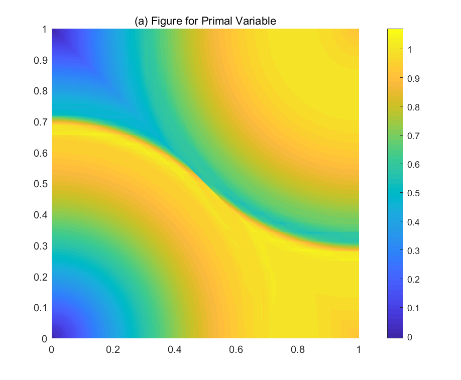
Refer to caption
Refer to caption
Refer to caption
Refer to caption
Fig. 2: Contour plots for numerical solutions with k=2π‘˜2k=2 and j=kβˆ’1π‘—π‘˜1j=k-1 on Ξ©1subscriptΞ©1\Omega_{1}, (a) the primal variable uhsubscriptπ‘’β„Žu_{h} and (b) the Lagrange multiplier Ξ»0subscriptπœ†0\lambda_{0} for f=0𝑓0f=0, (c) the primal variable uhsubscriptπ‘’β„Žu_{h} and (d) the Lagrange multiplier Ξ»0subscriptπœ†0\lambda_{0} for f=1𝑓1f=1, the coefficients {p,ρ,Ο„}={1.2,1,0}π‘πœŒπœ1.210\{p,\rho,\tau\}=\{1.2,1,0\}.
Refer to caption
Refer to caption
Refer to caption
Refer to caption
Fig. 3: Contour plots for numerical solutions with k=2π‘˜2k=2 and j=kβˆ’1π‘—π‘˜1j=k-1 on Ξ©1subscriptΞ©1\Omega_{1}, (e) the primal variable uhsubscriptπ‘’β„Žu_{h} and (f) the Lagrange multiplier Ξ»0subscriptπœ†0\lambda_{0} for f=0𝑓0f=0, (g) the primal variable uhsubscriptπ‘’β„Žu_{h} and (h) the Lagrange multiplier Ξ»0subscriptπœ†0\lambda_{0} for f=1𝑓1f=1, the coefficients {p,ρ,Ο„}={5,1​e+12,0}π‘πœŒπœ51𝑒120\{p,\rho,\tau\}=\{5,1e+12,0\}.

Figures 4-5 illustrate some contour plots for the primal variable uhsubscriptπ‘’β„Žu_{h} and the dual variable Ξ»0subscriptπœ†0\lambda_{0} in Ξ©1subscriptΞ©1\Omega_{1} for k=2π‘˜2k=2 and j=kβˆ’1π‘—π‘˜1j=k-1 when p=1.2𝑝1.2p=1.2 and p=5𝑝5p=5 are employed. The convection vector is given by 𝜷=[0.5βˆ’y,xβˆ’0.5]𝜷0.5𝑦π‘₯0.5{\boldsymbol{\beta}}=[0.5-y,x-0.5], and the reaction coefficient is c=1𝑐1c=1. The inflow boundary data is g=cos⁑(π​x)​cos⁑(π​y)π‘”πœ‹π‘₯πœ‹π‘¦g=\cos(\pi x)\cos(\pi y). The left ones in Figures 4-5 show the contour plots of the primal variable uhsubscriptπ‘’β„Žu_{h} corresponding to the load functions f=0𝑓0f=0 and f=1𝑓1f=1 respectively; while the right ones are the contour plots of the dual variable Ξ»0subscriptπœ†0\lambda_{0} for the load functions f=0𝑓0f=0 and f=1𝑓1f=1 respectively. Note that the exact solution of primal variable is unknown.

Refer to caption
Refer to caption
Refer to caption
Refer to caption
Fig. 4: Contour plots for numerical solutions with k=2π‘˜2k=2 and j=kβˆ’1π‘—π‘˜1j=k-1 on Ξ©1subscriptΞ©1\Omega_{1}, (a) the primal variable uhsubscriptπ‘’β„Žu_{h} and (b) the Lagrange multiplier Ξ»0subscriptπœ†0\lambda_{0} for f=0𝑓0f=0, (c) the primal variable uhsubscriptπ‘’β„Žu_{h} and (d) the Lagrange multiplier Ξ»0subscriptπœ†0\lambda_{0} for f=1𝑓1f=1, the coefficients {p,ρ,Ο„}={1.2,1,0}π‘πœŒπœ1.210\{p,\rho,\tau\}=\{1.2,1,0\}.
Refer to caption
Refer to caption
Refer to caption
Refer to caption
Fig. 5: Contour plots for numerical solutions with k=2π‘˜2k=2 and j=kβˆ’1π‘—π‘˜1j=k-1 on Ξ©1subscriptΞ©1\Omega_{1}, (e) the primal variable uhsubscriptπ‘’β„Žu_{h} and (f) the Lagrange multiplier Ξ»0subscriptπœ†0\lambda_{0} for f=0𝑓0f=0, (g) the primal variable uhsubscriptπ‘’β„Žu_{h} and (h) the Lagrange multiplier Ξ»0subscriptπœ†0\lambda_{0} for f=1𝑓1f=1, the coefficients {p,ρ,Ο„}={5,1​e+12,0}π‘πœŒπœ51𝑒120\{p,\rho,\tau\}=\{5,1e+12,0\}.

Figures 6-7 show the contour plots for the primal variable uhsubscriptπ‘’β„Žu_{h} and the dual variable Ξ»0subscriptπœ†0\lambda_{0} in the domain Ξ©2subscriptΞ©2\Omega_{2} for the load function f=0𝑓0f=0 and f=1𝑓1f=1 respectively. The configuration of this test problem is as follows: (1) the convection vector is piece-wisely defined such that 𝜷=[y+1,βˆ’xβˆ’1]πœ·π‘¦1π‘₯1{\boldsymbol{\beta}}=[y+1,-x-1] if y<1βˆ’x𝑦1π‘₯y<1-x and 𝜷=[yβˆ’2,2βˆ’x]πœ·π‘¦22π‘₯{\boldsymbol{\beta}}=[y-2,2-x] otherwise; (2) the reaction coefficient is c=0𝑐0c=0; (3) the inflow boundary data is g=cos⁑(5​y)𝑔5𝑦g=\cos(5y); (4) k=2π‘˜2k=2 and j=kβˆ’1π‘—π‘˜1j=k-1. We take p=1.2𝑝1.2p=1.2 and p=5𝑝5p=5. No exact solution of primal variable is known.
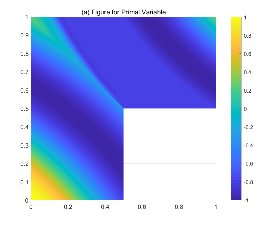
Refer to caption
Refer to caption
Refer to caption
Refer to caption
Fig. 6: Contour plots for numerical solutions with k=2π‘˜2k=2 and j=kβˆ’1π‘—π‘˜1j=k-1 on Ξ©2subscriptΞ©2\Omega_{2}, (a) the primal variable uhsubscriptπ‘’β„Žu_{h} and (b) the Lagrange multiplier Ξ»0subscriptπœ†0\lambda_{0} for f=0𝑓0f=0, (c) the primal variable uhsubscriptπ‘’β„Žu_{h} and (d) the Lagrange multiplier Ξ»0subscriptπœ†0\lambda_{0} for f=1𝑓1f=1, the coefficients {p,ρ,Ο„}={1.2,1,0}π‘πœŒπœ1.210\{p,\rho,\tau\}=\{1.2,1,0\}.
Refer to caption
Refer to caption
Refer to caption
Refer to caption
Fig. 7: Contour plots for numerical solutions with k=2π‘˜2k=2 and j=kβˆ’1π‘—π‘˜1j=k-1 on Ξ©2subscriptΞ©2\Omega_{2}, (e) the primal variable uhsubscriptπ‘’β„Žu_{h} and (f) the Lagrange multiplier Ξ»0subscriptπœ†0\lambda_{0} for f=0𝑓0f=0, (g) the primal variable uhsubscriptπ‘’β„Žu_{h} and (h) the Lagrange multiplier Ξ»0subscriptπœ†0\lambda_{0} for f=1𝑓1f=1, the coefficients {p,ρ,Ο„}={5,1​e+12,0}π‘πœŒπœ51𝑒120\{p,\rho,\tau\}=\{5,1e+12,0\}.

References

  • [1] A. N. Brooks and T. J. R. Hughes, Streamline upwind/Petrov-Galerkin formulations for convection dominated flows with particular emphasis on the incompressible Navier-Stokes equations, Comput. Methods Appl. Mech. Engrg., vol. 32 (1), pp. 199-259, 1982.
  • [2] E. Burman, Stabilized finite element methods for nonsymmetric, noncoercive, and ill-possed problems. Part II: hyperbolic equations, SIAM J. Sci. Comput., vol. 36 (4), pp. A1911-A1936, 2014.
  • [3] E. Burman and P. Hansbo, Edge stabilization for Galerkin approximations of convection-diffusion-reaction problems, Comput. Methods Appl. Mech. Engrg., vol. 193, pp. 1437-1453, 2004.
  • [4] E. Burman, A unified analysis for conforming and nonconforming stabilized finite element methods using interior penalty, SIAM J. Numer. Anal., vol. 43 (5), pp. 2012-2033, 2005.
  • [5] F. Brezzi, L. D. Marini, and E. SΓΌli, Discontinuous Galerkin methods for first-order hyperbolic problems, Math. Models Methods Appl. Sci., vol. 14 (12), pp. 1893-1903, 2004.
  • [6] E. Burman, A. Quarteroni, and B. Stamm, Interior penalty continuous and discontinuous finite element approximations of hyperbolic equations, J. Sci. Comput., vol. 43, pp. 293-312, 2010.
  • [7] E. Burman and B. Stamm, Minimal stabilization for discontinuous Galerkin finite element methods for hyperbolic problems, J. Sci. Comput., vol. 33, pp. 183-208, 2007.
  • [8] R. Becker and M. Braack, A two-level stabilization scheme for the Navier-Stokes equations, Numer. Math. Adv. Appl., Springer, Berlin, pp. 123-130, 2004.
  • [9] P. Bochev and J. Choi, Improved least-squares error estimates for scalar hyperbolic problems, Comput. Methods Appl. Math., vol. 1, pp. 115-124, 2001.
  • [10] G. Carey and B. Jiang, Least-squares finite elements for first-order hyperbolic systems, Int. J. Numer. Methods Eng., vol. 26, pp. 81-93, 1988.
  • [11] B. Cockburn, Discontinuous Galerkin methods for convection-dominated problems, in: High-Order Methods for Computational Physics, in: Lect. Notes Comput. Sci. Eng., vol. 9, Springer, Berlin, pp. 69-224, 1999.
  • [12] B. Cockburn and C. Shu, Runge-Kutta discontinuous Galerkin methods for convection-dominated problems, J. Sci. Comput., vol. 16 (3), pp. 173-261, 2001.
  • [13] W. Cao, C. Wang and J. Wang, An Lpsuperscript𝐿𝑝L^{p}-primal-dual weak Galerkin method for convection-diffusion equations, J. Comput. Appl. Math., vol. 419, pp. 114698, 2023.
  • [14] W. Cao, J. Wang and Y. Xu, An Lpsuperscript𝐿𝑝L^{p}-weak Galerkin method for second order elliptic equations in non-divergence form, arxiv. 2106.03191v1.
  • [15] S. Cao, C. Wang and J. Wang, A new numerical method for div-curl systems with low regularity assumptions, Comput. Math. Appl., vol. 114, pp. 47-59, 2022.
  • [16] W. Cao, C. Wang and J. Wang, An Lpsuperscript𝐿𝑝L^{p}-primal-dual weak Galerkin method for div-curl systems, J. Comput. Appl. Math., vol. 422, pp. 114881, 2023.
  • [17] R. Codina, Stabilization of incompressibility and convection through orthogonal sub-scales in finite element methods, Comput. Methods Appl. Mech. Engrg., vol. 190, pp. 1579-1599, 2000.
  • [18] J. L. Guermond, Stabilization of Galerkin approximations of transport equations by subgrid modeling, M2AN Math. Model. Numer. Anal., vol. 33, pp. 1293-1316, 1999.
  • [19] P. Houston, M. Jensen and E. Suli, Hp-discontinuous Galerkin finite element methods with least-squares stabilization, J. Sci. Comput., vol. 17, pp. 3-25, 2002.
  • [20] C. Johnson, U. NΓ€vert and J. PitkΓ€ranta, Finite element methods for linear hyperbolic problems, Comput. Methods Appl. Mech. Engrg., vol. 45, pp. 285-312, 1984.
  • [21] C. Johnson and J. PitkΓ€ranta, An analysis of the discontinuous Galerkin method for a scalar hyperbolic equation, Math. Comp., vol. 46, pp. 1-26, 1986.
  • [22] D. Li, C. Wang and J. Wang, A primal-dual finite element method for transport equations in non-divergence form, J. Comput. Appl. Math., vol. 412, pp. 114313, 2022.
  • [23] L. Mu and X. Ye, A simple finite element method for linear hyperbolic problems, J. Comput. Appl. Math., vol. 330, pp. 330-339, 2018.
  • [24] W. Reed and T. Hill, Triangular mesh methods for the neutron transport equation, Tech. Report LAUR-73-479, Los Alamos Scientific Laboratory, 1973.
  • [25] H. Sterck, T. Manteuffel, S. Mccormick and L. Olson, Least-squares finite element methods and algebraic multigrid solvers for linear hyperbolic PDEs, SIAM J. Sci. Comput., vol. 26 (1), pp. 31-54, 2005.
  • [26] C. Vogel and M. Oman, Iterative methods for total variation denoising, SIAM J. Sci. Comput., vol. 17, pp. 227-238, 1996.
  • [27] C. Wang and J. Wang, A primal-dual finite element method for first-order transport problems, J. Comput. Phys., vol. 417, pp. 109571, 2020.
  • [28] C. Wang and J. Wang, A primal-dual weak Galerkin finite element method for second order elliptic equations in non-divergence form, Math. Comp., vol. 87, pp. 515-545, 2018.
  • [29] J. Wang and X. Ye, A weak Galerkin finite element method for second-order elliptic problems, J. Comput. Appl. Math., vol. 241, pp. 103-115, 2013.
  • [30] J. Wang and X. Ye, A weak Galerkin mixed finite element method for second-order elliptic problems, Math. Comp., vol. 83, pp. 2101-2126, 2014.
  • [31] C. Wang and J. Wang, A primal-dual weak Galerkin finite element method for second order elliptic equations in non-divergence form, Math. Comp., vol. 87, pp. 515-545, 2018.
  • [32] C. Wang and J. Wang, A primal-dual weak Galerkin finite element method for Fokker-Planck type equations, SIAM J. Numer. Anal., vol. 58 (5), pp. 2632-2661, 2020.
  • [33] C. Wang and J. Wang, Primal-dual weak Galerkin finite element methods for elliptic Cauchy problems, Comput. Math. Appl., vol. 79 (3), pp. 746-763, 2020.
  • [34] C. Wang, A new primal-dual weak Galerkin finite element method for Ill-posed elliptic Cauchy problems, J. Comput. Appl. Math., vol. 371, pp. 112629, 2020.
  • [35] C. Wang and L. Zikatanov, Low regularity primal-dual weak Galerkin finite element methods for convection-diffusion equations, J. Comput. Appl. Math., vol. 394, 113543, 2021.