Runtime Performance of Evolutionary Algorithms for the Chance-constrained Makespan Scheduling Problem

Abstract

The Makespan Scheduling problem is an extensively studied NP-hard problem, and its simplest version looks for an allocation approach for a set of jobs with deterministic processing time to two identical machines such that the makespan is minimized. However, in real life scenarios, the actual processing time of each job may be stochastic around the expected value with a variance, under the influence of external factors, and the actual processing time of these jobs may be correlated with covariances. Thus within this paper, we propose a chance-constrained version of the Makespan Scheduling problem and investigate the theoretical performance of the classical Randomized Local Search and (1+1) EA for it. More specifically, we study three variants of the Chance-constrained Makespan Scheduling problem and their computational complexities, then separately analyze the expected runtime of the two algorithms to obtain an optimal solution or almost optimal solution to the instances of the three variants. In addition, we investigate the experimental performance of the two algorithms for the three variants.

Keywords

Chance-constraint, Makespan Scheduling problem, RLS, (1+1) EA.

1 Introduction

Background. To discover the reasons behind the successful applications of evolutionary algorithms in various areas including engineering, logistics and economics, lots of researchers made efforts to study the theoretical performance of evolutionary algorithms for classical combinatorial optimization problems. However, most of these combinatorial optimization problems studied for the theoretical performance of evolutionary algorithms are deterministic (such as Minimum Spanning Tree problem (Neumann and Wegener,, 2006, 2007; Kratsch et al.,, 2010; Corus et al.,, 2013; Witt,, 2014; Vahid et al.,, 2020), Vertex Cover problem (Oliveto et al.,, 2008, 2009; Friedrich et al.,, 2009, 2010; Yu et al.,, 2012; Jansen et al.,, 2013; Kratsch and Neumann,, 2013; Pourhassan et al.,, 2015, 2016, 2017), and Knapsack problem (Kumar and Banerjee,, 2005; He et al.,, 2014, 2015; Wu et al.,, 2016; Neumann and Sutton,, 2018; Roostapour et al.,, 2018; Friedrich et al.,, 2020)), and the combinatorial optimization problems in real-world are often stochastic and have dynamic components. Hence in the past few years, some related researchers paid attention to the theoretical performance of evolutionary algorithms for dynamic and stochastic combinatorial optimization problems (He et al.,, 2014; Lissovoi and Witt,, 2017; Shi et al.,, 2019; Neumann et al.,, 2020; Shi et al.,, 2021; Roostapour et al.,, 2022) and obtained a series of theoretical results that further advance and broaden the understanding of evolutionary algorithms.

Chance-constrained optimization problems are an important class of stochastic optimization problems. They consider that the constraints of the given optimization problem may be influenced by the noise of stochastic components, thus the goal is to optimize the objective function under that the constraints can be violated up to certain probability levels (Charnes and Cooper,, 1959; Miller and Wagner,, 1965; Iwamura and Liu,, 1996; Poojari and Varghese,, 2008). The basic technique for solving chance-constrained optimization problems is to convert the stochastic constraints to their respective deterministic equivalents according to the predetermined confidence level. Recently, some researchers in the area of evolutionary computing began to focus on chance-constrained optimization problems and analyze the theoretical performance of evolutionary algorithms for them.

The Makespan Scheduling problem (abbr. MSP) (Blazewicz et al.,, 1983) is one of the most popular combinatorial optimization problems and has been well-studied particularly in the area of theoretical computer science. The problem considers two identical machines and a set of jobs with deterministic processing time, and its aim is to allocate the jobs to the two machines such that the makespan (i.e., completion time) to finish all these jobs is minimized (specifically, the makespan is the larger one of the loads on the two machines, where the load on a machine is the sum of the processing time of the jobs allocated to it). In real life scenarios, the actual processing time of each job may be stochastic around the expected value with a variance, under the influence of external factors. Moreover, the actual processing time of these jobs may be correlated with covariances. Therefore, a chance-constrained version of MSP, named Chance-constrained Makespan Scheduling Problem (abbr. CCMSP), is proposed in the paper. CCMSP considers two identical machines and several groups of jobs, where the jobs in the same group have the same expected processing time and variance, and their actual processing time are correlated by a covariance if they are allocated to the same machine (i.e., the actual processing time of two jobs in the same group are independent if they are allocated to different machines, and that of the jobs in different groups are independent). The goal of CCMSP is to minimize a deterministic makespan value and subject to the probability that the actual makespan exceeds the deterministic makespan is no more than an acceptable threshold.

Related work. In the previous research, a few theoretical results have been obtained about the performance of evolutionary algorithms for MSP and chance-constrained problems. One of the first runtime analysis of evolutionary algorithms for MSP with two identical machines was carried out by Witt, (2005), who studied the approximation and average-case behavior of Randomized Local Search (abbr. RLS) and the (1+1) EA for the problem. Later Gunia, (2005) extended the results to MSP with a constant number of identical machines. Sutton and Neumann, (2012) gave the parameterized runtime analysis of RLS and the (1+1) EA for MSP with two identical machines, with respect to three different parameters. Neumann and Witt, (2015) proposed the dynamic version of MSP with two identical machines and analyzed the performance of RLS and the (1+1) EA for it.

Xie et al., (2019) studied single- and multi-objective evolutionary algorithms for the Chance-constrained Knapsack problem, where the weights of items are stochastic but the profits are deterministic, and they used the Chebyshev’s inequality and Chernoff bound separately to estimate the constraint violation probability of a given solution. Then Neumann and Sutton, (2019) followed the work of Xie et al., (2019) and analyzed several special cases of this problem, getting insight into how the structure of the chance constraint influences the runtime behavior of the (1+1) EA. Note that the Chance-constrained Knapsack problem studied in the above two works does not consider the correlationship among the weights of items. Thus recently Xie et al., (2021) extended their work and analyzed the expected optimization time of RLS and the (1+1) EA for the Chance-constrained Knapsack Problem with correlated uniform weights. Additionally, Neumann and Neumann, (2020) presented the first runtime analysis of multi-objective evolutionary algorithms for chance-constrained submodular functions, and showed that the algorithm GSEMO obtains the same worst case performance guarantees as greedy algorithms (Doerr et al.,, 2020).

Besides these theoretical works, Xie et al., (2020) introduced a problem-specific crossover operator and the heavy-tail mutation operator (Doerr et al.,, 2017) to evolutionary algorithms to improve their performance for the Chance-constrained Knapsack problem, and compared their experimental performance. Moreover, Assimi et al., (2020) studied the experimental performance of a single-objective EA for the dynamic version of the Chance-constrained Knapsack problem, where each item has an uncertain weight while its profit is deterministic, and the knapsack capacity changes over time every a constant number of iterations. Recently, Neumann et al., (2022) considered another chance-constrained version of the Knapsack problem, where the weights of items are deterministic but the profits are stochastic. Within their investigation, they used the Chebyshev’s inequality and Hoeffding bound separately to estimate the constraint violation probability of a given solution, and examined three evolutionary algorithms of different types and compared their experimental performance on the problem.

Our contribution. Within this paper, we investigate the expected runtime of RLS and the (1+1) EA for CCMSP. More specifically, we consider two special variants of CCMSP: (1). CCMSP-1, all jobs have the same expected processing time and variance, and all groups have the same covariance and the same even size; (2). CCMSP-2, all jobs have the same expected processing time and variance, the groups have the same covariance but different sizes. For CCMSP-1, we prove that it is polynomial-time solvable by showing that RLS and the (1+1) EA can obtain an optimal solution to any instance $I_{1}$ of CCMSP-1 in expected runtime $O(n^{2}/m)$ and $O((k+m)n^{2})$, respectively, where $n$ and $k$ are the numbers of jobs and groups considered in $I_{1}$, and $m=n/k$. For CCMSP-2, the size difference among groups makes the discussion complicated, thus two simplified variants of CCMSP-2 named CCMSP-2⁺ and CCMSP-2^- are proposed: CCMSP-2⁺ assumes that the sum of the variances and covariances of the jobs allocated to the same machine cannot be over the expected processing time of a job, no matter how many jobs are allocated to the machine; CCMSP-2^- assumes that the sum of the variances and expected processing time of the jobs cannot be over their covariances. We prove that CCMSP-2⁺ is surprisingly NP-hard and that RLS can obtain an optimal solution to any instance $I_{2}^{+}$ of CCMSP-2⁺ in expected polynomial-runtime if the total number of jobs considered in $I_{2}^{+}$ is odd; otherwise (i.e., the total number of jobs considered is even), a solution close to the optimal one to $I_{2}^{+}$. We show that CCMSP-2^- is NP-hard as well and analyze the approximation ratio of the local optimal solution obtained by RLS.

In addition, we study the experimental performance of the two algorithms. For each variant, we specify a parameter-triple $(k,n,c)$, in which $c$ has 3 settings, and each of $k$ and $n$ has 6 settings (i.e., there are 108 instance of each variant that are constructed). Then we study the number of iterations that the algorithms RLS and the (1+1) EA require to get an optimal or local optimal solution for each instance, and find that the experimental results coincide with the theoretical ones obtained for them. Specifically, for each constructed instance $I$ of CCMSP-2⁺ with even many jobs, a corresponding instance $I^{\prime}$ of CCMSP-2⁺ with odd many jobs is constructed by introducing an extra job to an arbitrary group of $I$, for ease of comparison. The experimental result shows that the tiny difference between the two instances causes a huge gap between the experimental performance of RLS on them, which coincides with the computational hardness of CCMSP-2⁺ with odd many jobs mentioned above.

This paper extends and refines the conference version (Shi et al.,, 2022). Firstly, the study of CCMSP-2^- and the experimental analysis of the two algorithms are newly added (Subsection 5.3 and Section 6). Secondly, the theoretical performance of RLS for the instances of CCMSP-2⁺ with even many jobs is rewritten (Subsection 5.2). Finally, more details and illustrations for the theoretical performance of the two algorithms are included (e.g., Section 4 and Section 5).

The paper is structured as follows. Section 2 introduces the related definitions and the formulation of CCMSP. Section 3 presents the two considered algorithms, namely, RLS and the (1+1) EA, and Section 4 analyzes their theoretical performance to obtain an optimal solution to the instances of CCMSP-1. Then Section 5 considers the theoretical performance of RLS for solving the instances of CCMSP-2⁺ and CCMSP-2^-. The experimental performance of RLS and the (1+1) EA for CCMSP-1, CCMSP-2⁺ and CCMSP-2^- is studied in Section 6. Section 7 is used to conclude this work.

2 Preliminaries

The notation $[x,y]$ ($x$ and $y$ are two integers with $x\leq y$) denotes the set containing all integers ranging from $x$ to $y$. Let $[x,y)=[x,y]\setminus\{y\}$ and $(x,y]=[x,y]\setminus\{x\}$. Consider two identical machines $M_{0}$ and $M_{1}$, and $k$ groups of jobs, where each group $G_{i}$ ($i\in[1,k]$) has $m_{i}$ many jobs. That is, there are $n=\sum_{i=1}^{k}m_{i}$ many jobs in total. W.l.o.g., assume that the sizes of the $k$ groups are in non-decreasing order (i.e., $m_{1}\leq m_{2}\leq\ldots\leq m_{k}$). The $j$-th job in group $G_{i}$ ($i\in[1,k]$ and $j\in[1,m_{i}]$), denoted by $b_{ij}$, has actual processing time $p_{ij}$ with expected value $E[p_{ij}]=a_{ij}>0$ and variance $\sigma^{2}_{ij}\geq 0$. Additionally, for any two jobs of the same group $G_{i}$, if they are allocated to the same machine, then their actual processing time are correlated with each other by a covariance $c_{i}\geq 0$; otherwise, independent.

The Chance-constrained Makespan Scheduling Problem (abbr. CCMSP) studied in the paper looks for an allocation of the $n$ many jobs to the two machines that minimizes the makespan $M$ such that the probabilities of the loads on $M_{0}$ and $M_{1}$ exceeding $M$ are no more than a given acceptable threshold $0\leq\gamma<1$, where the load on $M_{t}$ ($t\in[0,1]$) is the sum of the actual processing time of the jobs allocated to $M_{t}$.

An allocation (or simply called solution in the remaining text) $x$ to an instance of CCMSP, is represented as a bit-string with length $n$ in this paper, $x=x_{11}...x_{1m_{1}}...x_{i1}...x_{im_{i}}...x_{k1}...x_{km_{k}}\in\{0,1\}^{n}$, where the job $b_{ij}$ is allocated to machine $M_{0}$ if $x_{ij}=0$; otherwise, allocated to machine $M_{1}$ (in the remaining text, we simply say that a bit is of $G_{i}$ if its corresponding job is of $G_{i}$). For ease of notation, denote by $M_{t}(x)$ the set of jobs allocated to $M_{t}$ ($t\in[0,1]$), with respect to $x$, and by $l_{t}(x)=\sum_{b_{ij}\in M_{t}(x)}p_{ij}$ the load on $M_{t}$. Let $\alpha_{i}(x)=|M_{0}(x)\cap G_{i}|$ and $\beta_{i}(x)=|M_{1}(x)\cap G_{i}|$ for all $i\in[1,k]$. The CCMSP can be formulated as:

$$\textbf{Minimize}\qquad M$$

$$\textbf{Subject to}\quad\Pr(l_{t}(x)>M)\leq\gamma\ \ \textrm{for all}\ \ t\in[0,1].$$

Since $E[p_{ij}]=a_{ij}$, the excepted value of $l_{t}(x)$ is $E[l_{t}(x)]=\sum_{b_{ij}\in M_{t}(x)}a_{ij}$. Considering the variance $\sigma^{2}_{ij}$ of each job $b_{ij}$ and the covariance among the jobs of the same group if they are allocated to the same machine, the variance of $l_{t}(x)$ is

$$var[l_{t}(x)]=\sum_{b_{ij}\in M_{t}(x)}\sigma^{2}_{ij}+cov[l_{t}(x)],\ {\rm where}\ cov[l_{t}(x)]=\sum_{i=1}^{k}2c_{i}\times\binom{|M_{t}(x)\cap G_{i}|}{2}.$$

Note that $\binom{|M_{t}(x)\cap G_{i}|}{2}=0$ if $0\leq|M_{t}(x)\cap G_{i}|\leq 1$.

For the probability $Pr(l_{t}(x)>M)$ with $t\in[0,1]$, following the work of Xie et al., (2019, 2021), we use the One-sided Chebyshev’s Inequality (cf. Theorem 1) to construct a usable surrogate of the chance-constraint.

Theorem 1.

(One-sided Chebyshev’s Inequality). Let $X$ be a random variable with expected value $E[X]$ and variance $var[X]$. Then for any $\Delta\in\mathbb{R}^{+}$,

$$\Pr(X>E[X]+\Delta)\leq\frac{var[X]}{var[X]+\Delta^{2}}.$$

By the One-sided Chebyshev’s Inequality, upper bounding the probability of the actual makespan exceeding $M$ by $\gamma$ indicates that for all $t\in[0,1]$,

$$\Pr(l_{t}(x)>M) \leq\frac{var[l_{t}(x)]}{var[l_{t}(x)]+(M-E[l_{t}(x)])^{2}}\leq\gamma$$

$$\iff \sqrt{\frac{(1-\gamma)}{\gamma}var[l_{t}(x)]}+E[l_{t}(x)]=l^{\prime}_{t}(x)\leq M.$$

Note that as the value of $\Delta$ considered in the One-sided Chebyshev’s Inequality is positive, thus $M-E[l_{t}(x)]$ is greater than 0 by default, and the left right double arrow (i.e., the if and only if relationship) given in the above expression holds. Summarizing the above analysis gets that $\max\{\Pr(l_{0}(x)>M),\Pr(l_{1}(x)>M)\}\leq\gamma$ holds if and only if

$$L(x)=\max\{l_{0}^{\prime}(x),l_{1}^{\prime}(x)\}\leq M.$$

In other words, $L(x)$ is the tight lower bound for the value of $M$, if using the surrogate of the chance-constraint by the One-sided Chebyshev’s Inequality. Consequently, $l^{\prime}_{t}(x)$ can be treated as a new measure for the load on the machine $M_{t}$, and the goal of CCMSP is simplified to minimize the value of $L(x)$. Let $t(x)=\arg\max_{t\in[0,1]}\{l_{0}^{\prime}(x),l_{1}^{\prime}(x)\}$.

It is easy to derive that CCMSP is NP-hard, as CCMSP is the same as MSP if $\sigma^{2}_{ij}=c_{i}=0$ for all $i\in[1,k]$ and $j\in[1,m_{i}]$, and $\gamma=0$. Witt, (2005) showed that the classical RLS and the (1+1) EA for MSP may get trapped into a bad local optima caused by the different processing time of the jobs considered, such that they require $O(n^{\Omega(n)})$ runtime to escape it. Observe that the same issue also applies to the two algorithms for CCMSP. Thus within the paper, we only study the two specific variants of CCMSP given below, in which the jobs considered have the same expected processing time.

CCMSP-1. All the $n$ many jobs considered have the same expected processing time $a_{ij}=a>0$ and variance $\sigma^{2}_{ij}=d\geq 0$, and the $k$ groups have the same covariance $c\geq 0$ and size $m>0$ (i.e., $c_{i}=c$ and $m_{i}=m$ for all $i\in[1,k]$). Moreover, $m$ is even.

CCMSP-2. All the $n$ many jobs considered have the same expected processing time $a_{ij}=a>0$ and variance $\sigma^{2}_{ij}=d>0$, and the $k$ groups have the same covariances $c\geq 0$ (i.e., $c_{i}=c$ for all $i\in[1,k]$). However, the $k$ groups may have different sizes (may be even or odd).

Given an instance $I$ of CCMSP-1 or CCMSP-2 and an arbitrary solution $x$ to $I$, if $||M_{0}(x)|-|M_{1}(x)||\leq 1$ (i.e., $|M_{0}(x)|=|M_{1}(x)|$ if $n$ is even), then $x$ is an equal-solution; if $||M_{0}(x)|-|M_{1}(x)||\leq 1$, and $|\alpha_{i}(x)-\beta_{i}(x)|\leq 1$ for all $i\in[1,k]$ (i.e., $\alpha_{i}(x)=\beta_{i}(x)$ if $m_{i}$ is even), then $x$ is a balanced-solution.

3 Algorithms

Within the paper, we study the performance of the classical Randomized Local Search (abbr. RLS, given as Algorithm 1) and (1+1) EA (given as Algorithm 2) for the two variants of CCMSP. The two algorithms run in a similar way, randomly generating a new offspring based on the current maintained solution and replacing it if the offspring is not worse than it in terms of their fitness. The difference between the two algorithms is the way to generate offspring: With probability 1/2, RLS chooses one bit of the current maintained solution uniformly at random and flips it, and 1/2 chooses two bits of the current maintained solution uniformly at random and flips them; the (1+1) EA flips each bit of the current maintained solution with probability $1/n$.

The fitness function considered in the two algorithms is the natural one,

$$f(x)=L(x)=\max\{l_{0}^{\prime}(x),l_{1}^{\prime}(x)\}.$$

1 choose $x\in\{0,1\}^{n}$ uniformly at random;

2 while stopping criterion not met do

3       choose $b\in\{0,1\}$ uniformly at random;

4       if $b=0$ then

5             $y$ $\leftarrow$ flip one bit of $x$ chosen uniformly at random;

6       end if

7      else

8            choose $(i,j)\in\{(k,l)|1\leq k<l\leq n\}$ uniformly at random;

9             $y$ $\leftarrow$ flip the $i$-th and $j$-th bits of $x$;

10       end if

11      if $f(y)\leq f(x)$ then

12            $x\leftarrow y$;

13       end if

14      

15 end while

Algorithm 1 RLS

1 choose $x\in\{0,1\}^{n}$ uniformly at random;

2 while stopping criterion not met do

3       $y$ $\leftarrow$ flip each bit of $x$ independently with probability $1/n$;

4       if $f(y)\leq f(x)$ then

5            $x\leftarrow y$;

6       end if

7      

8 end while

Algorithm 2 (1+1) EA

4 Theoretical Performance for CCMSP-1

The section starts with an observation that will be used throughout the paper.

Observation 2.

$\binom{\lfloor\frac{x+y}{2}\rfloor}{2}+\binom{\lceil\frac{x+y}{2}\rceil}{2}\leq\binom{x}{2}+\binom{y}{2}\leq\binom{x+y}{2}$ holds for any two natural numbers $x$ and $y$.

Consider an instance $I_{1}=(a,c,d,\gamma,k,m)$ of CCMSP-1 and a solution $x$ to $I_{1}$. As the groups considered in $I_{1}$ have the same size $m$, there is a variable $0\leq\delta_{i}(x)\leq\frac{m}{2}$ such that $\alpha_{i}(x)=\frac{m}{2}+\delta_{i}(x)$ and $\beta_{i}(x)=\frac{m}{2}-\delta_{i}(x)$ for any $i\in[1,k]$, and it is easy to get the following lemma.

Lemma 3.

For any solution $x$ to the instance $I_{1}=(a,c,d,\gamma,k,m)$ of CCMSP-1, if $|M_{0}(x)|>|M_{1}(x)|$ (resp., $|M_{1}(x)|>|M_{0}(x)|$) then $l^{\prime}_{0}(x)>l^{\prime}_{1}(x)$ (resp., $l^{\prime}_{1}(x)>l^{\prime}_{0}(x)$); if $x$ is an equal-solution then $L(x)=l^{\prime}_{0}(x)=l^{\prime}_{1}(x)$.

Proof.

First of all, we show the claim that if $|M_{0}(x)|>|M_{1}(x)|$ then $l^{\prime}_{0}(x)>l^{\prime}_{1}(x)$. Recall that all jobs have the same expected processing time $a$ and variance $d$, thus $E[l_{0}(x)]>E[l_{1}(x)]$ and

$$\sum_{b_{ij}\in M_{0}(x)}d>\sum_{b_{ij}\in M_{1}(x)}d.$$ (1)

Now we show that $cov[l_{0}(x)]>cov[l_{1}(x)]$, i.e.,

$$\binom{\alpha_{1}}{2}+\ldots+\binom{\alpha_{k}}{2}>\binom{\beta_{1}}{2}+\ldots+\binom{\beta_{k}}{2}.$$ (2)

For any specific $i\in[1,k]$, $\binom{\alpha_{i}}{2}-\binom{\beta_{i}}{2}=\binom{m/2+\delta_{i}}{2}-\binom{m/2-\delta_{i}}{2}=(m-1)\delta_{i}$. Then

$$\begin{aligned} \sum_{i=1}^{k}\left(\binom{\alpha_{i}}{2}-\binom{\beta_{i}}{2}\right)&=\sum_{i=1}^{k}(m-1)\delta_{i}=(m-1)\sum_{i=1}^{k}\delta_{i}\\ &=\frac{m-1}{2}\left(\sum_{i=1}^{k}\alpha_{i}(x)-\sum_{i=1}^{k}\beta_{i}(x)\right)\\ &=\frac{m-1}{2}\left(|M_{0}(x)|-|M_{1}(x)|\right)>0.\end{aligned}$$ (3)

Thus Inequality (2) holds. Combining Inequalities (1) and (2) gives that $var[l_{0}(x)]>var[l_{1}(x)]$. As the considered threshold $\gamma$ is a fixed constant, summarizing the above discussion shows the claim. Because of symmetry, we can also derive that if $|M_{0}(x)|<|M_{1}(x)|$ then $l^{\prime}_{0}(x)<l^{\prime}_{1}(x)$.

Now we show that if $|M_{0}(x)|=|M_{1}(x)|$ then $l^{\prime}_{0}(x)=l^{\prime}_{1}(x)$. Observe that $E[l_{0}(x)]=E[l_{1}(x)]$, $\sum_{b_{ij}\in M_{0}(x)}d=\sum_{b_{ij}\in M_{1}(x)}d$ and $\sum_{i=1}^{k}\delta_{i}=0$. Combining $\sum_{i=1}^{k}\delta_{i}=0$ and Expression (3) gives that

$$\binom{\alpha_{1}}{2}+\ldots+\binom{\alpha_{k}}{2}=\binom{\beta_{1}}{2}+\ldots+\binom{\beta_{k}}{2}.$$

Therefore, $var[l_{0}(x)]=var[l_{1}(x)]$ and $l^{\prime}_{0}(x)=l^{\prime}_{1}(x)=L(x)$. ∎

Based on Lemma 3, we can get the following lemma.

Lemma 4.

For any solution $x$ to the instance $I_{1}=(a,c,d,\gamma,k,m)$ of CCMSP-1, if $x$ is a balanced-solution then $L(x)=l^{\prime}_{0}(x)=l^{\prime}_{1}(x)$ has the minimum value; more specifically, $x$ is an optimal solution to $I_{1}$ if and only if $x$ is a balanced-solution to $I_{1}$.

Proof.

To show that $L(x)=l^{\prime}_{0}(x)=l^{\prime}_{1}(x)$ has the minimum value if $\alpha_{i}=\beta_{i}=m/2$ for all $i\in[1,k]$, we first prove the claim that the minimum value of $L(x)$ if $|M_{0}(x)|\neq|M_{1}(x)|$ is larger than that of $L(x)$ if $|M_{0}(x)|=|M_{1}(x)|$.

For the minimum value of $L(x)$ if $|M_{0}(x)|\neq|M_{1}(x)|$, w.l.o.g., we assume that $|M_{0}(x)|>|M_{1}(x)|$, i.e., $\sum_{i=1}^{k}\delta_{i}\geq 1$. By Lemma 3, $L(x)=l^{\prime}_{0}(x)>l^{\prime}_{1}(x)$, and

$$cov[l_{0}(x)]/c = \sum_{i=1}^{k}\alpha_{i}(\alpha_{i}-1)=\sum_{i=1}^{k}(m/2+\delta_{i})^{2}-\sum_{i=1}^{k}(m/2+\delta_{i})$$

$$= km^{2}/4+(m-1)\sum_{i=1}^{k}\delta_{i}+\sum_{i=1}^{k}\delta_{i}^{2}-n/2$$

$$\geq km^{2}/4+(m-1)+1-n/2$$

$$\geq km^{2}/4+m-n/2.$$

Thus if $|M_{0}(x)|>|M_{1}(x)|$ then $var[l_{0}(x)]\geq d(n/2+1)+c(km^{2}/4+m-n/2)$ and

$$L(x)=l^{\prime}_{0}(x)\geq\sqrt{\frac{(1-\gamma)}{\gamma}\left(d(n/2+1)+c(km^{2}/4+m-n/2)\right)}+(n/2+1)a=A.$$

For the minimum value of $L(x)$ if $|M_{0}(x)|=|M_{1}(x)|$, we have that $\sum_{i=1}^{k}\delta_{i}=0$, $L(x)=l^{\prime}_{0}(x)=l^{\prime}_{1}(x)$ due to Lemma 3, and

$$cov[l_{0}(x)]/c=km^{2}/4+(m-1)\sum_{i=1}^{k}\delta_{i}+\sum_{i=1}^{k}\delta_{1}^{2}-n/2\geq km^{2}/4+0+0-n/2=km^{2}/4-n/2.$$ (4)

Thus if $|M_{0}(x)|=|M_{1}(x)|$ then $var[l_{0}(x)]\geq dn/2+c(km^{2}/4-n/2)$ and

$$L(x)=l^{\prime}_{0}(x)\geq\sqrt{\frac{(1-\gamma)}{\gamma}\left(dn/2+c(km^{2}/4-n/2)\right)}+na/2=B.$$

Obviously, $A>B$, thus the first claim is correct.

By Inequality (4), under the case that $|M_{0}(x)|=|M_{1}(x)|$, $L(x)$ gets its minimum value $B$ if $\delta_{i}=0$ for all $i\in[1,k]$. Consequently, the second claim that $x$ is a balanced-solution to $I_{1}$ if and only if $x$ is optimal to $I_{1}$ is correct. ∎

Figure 1: An illustration for the proof of Theorem 5.

Now we are ready to analyze the expected runtime of RLS and the (1+1) EA to solve CCMSP-1.

Theorem 5.

The expected runtime of RLS to obtain an optimal solution to the instance $I_{1}=(a,c,d,\gamma,k,m)$ of CCMSP-1 is $O(n^{2}/m)=O(kn)$.

Proof.

Lemma 4 shows that any optimal solution to $I_{1}$ is a balanced-one. Let $x_{0}$ be the initial solution maintained by RLS that is assumed to have $|M_{0}(x_{0})|>|M_{1}(x_{0})|$. Thus $L(x)=l^{\prime}_{0}(x_{0})>l^{\prime}_{1}(x_{0})$ by Lemma 3 and $|M_{0}(x_{0})|-|M_{1}(x_{0})|\geq 2$ as $n=mk$ is even. The optimization process of RLS based on $x_{0}$ discussed below is divided into two phases, illustrated in Fig. 1

Phase-1. Obtaining the first equal-solution $x_{1}$ based on $x_{0}$. Five possible cases for the mutation of RLS on $x_{0}$ are listed below, obtaining an offspring $x^{\prime}_{0}$ of $x_{0}$.

Case (1). Flipping a 0-bit in $x_{0}$ (i.e., $|M_{0}(x^{\prime}_{0})|=|M_{0}(x_{0})|-1$). Observe that $E[l_{0}(x_{0})]>E[l_{0}(x^{\prime}_{0})]$, $var[l_{0}(x_{0})]>var[l_{0}(x^{\prime}_{0})]$ and $l^{\prime}_{0}(x_{0})>l^{\prime}_{0}(x^{\prime}_{0})$, since a job on $M_{0}$ with respect to $x_{0}$ is moved to $M_{1}$. As $|M_{0}(x_{0})|-|M_{1}(x_{0})|\geq 2$ we have $|M_{0}(x^{\prime}_{0})|\geq|M_{1}(x^{\prime}_{0})|$. Thus $L(x^{\prime}_{0})=l^{\prime}_{0}(x^{\prime}_{0})$ by Lemma 3, $L(x^{\prime}_{0})=l^{\prime}_{0}(x^{\prime}_{0})<l^{\prime}_{0}(x_{0})=L(x_{0})$, and $x^{\prime}_{0}$ can be accepted by RLS.

Case (2). Flipping a 1-bit in $x_{0}$ (i.e., $|M_{0}(x^{\prime}_{0})|=|M_{0}(x_{0})|+1$). Since a job on $M_{1}$ with respect to $x_{0}$ is moved to $M_{0}$, $E[l_{0}(x^{\prime}_{0})]>E[l_{0}(x_{0})]$, $var[l_{0}(x^{\prime}_{0})]>var[l_{0}(x_{0})]$, and $l^{\prime}_{0}(x^{\prime}_{0})>l^{\prime}_{0}(x_{0})$. Similarly, $l^{\prime}_{1}(x_{0})>l^{\prime}_{1}(x^{\prime}_{0})$. Since $l^{\prime}_{0}(x_{0})>l^{\prime}_{1}(x_{0})$, $L(x^{\prime}_{0})=l^{\prime}_{0}(x^{\prime}_{0})>l^{\prime}_{0}(x_{0})=L(x_{0})$ and $x^{\prime}_{0}$ cannot be accepted by RLS.

Case (3). Flipping two 0-bits in $x_{0}$ (i.e., $|M_{0}(x^{\prime}_{0})|=|M_{0}(x_{0})|-2$). If $|M_{0}(x^{\prime}_{0})|\geq|M_{1}(x^{\prime}_{0})|$, then using the reasoning for Case (1) gets that $L(x^{\prime}_{0})\leq L(x_{0})$ and $x^{\prime}_{0}$ can be accepted by RLS. If $|M_{0}(x^{\prime}_{0})|<|M_{1}(x^{\prime}_{0})|$ then by the facts that $|M_{0}(x_{0})|-|M_{1}(x_{0})|\geq 2$ and $n$ is even, $|M_{0}(x_{0})|-|M_{1}(x_{0})|=2$, $|M_{1}(x^{\prime}_{0})|-|M_{0}(x^{\prime}_{0})|=2$ and $|M_{0}(x_{0})|=|M_{1}(x^{\prime}_{0})|$. By Lemma 3, we have

$$L(x_{0})-L(x^{\prime}_{0})=l^{\prime}_{0}(x_{0})-l^{\prime}_{1}(x^{\prime}_{0})=\sqrt{\frac{1-\gamma}{\gamma}}\left(\sqrt{var[l_{0}(x_{0})]}-\sqrt{var[l_{1}(x^{\prime}_{0})]}\right).$$

Recall that $|M_{0}(x_{0})|=|M_{1}(x^{\prime}_{0})|$, thus

$$\sqrt{var[l_{0}(x_{0})]}\geq\sqrt{var[l_{1}(x^{\prime}_{0})]}\ \Longleftrightarrow\ cov[l_{0}(x_{0})]\geq cov[l_{1}(x^{\prime}_{0})].$$

Consequently, $x^{\prime}_{0}$ can be accepted by RLS if and only if $cov[l_{0}(x_{0})]\geq cov[l_{1}(x^{\prime}_{0})]$.

Case (4). Flipping a 0-bit and a 1-bit in $x_{0}$ (i.e., $|M_{0}(x^{\prime}_{0})|=|M_{0}(x_{0})|$). Observe $|M_{0}(x_{0})|=|M_{0}(x^{\prime}_{0})|\geq|M_{1}(x^{\prime}_{0})|$. By Lemma 3,

$$L(x_{0})-L(x^{\prime}_{0})=l^{\prime}_{0}(x_{0})-l^{\prime}_{0}(x^{\prime}_{0})=\sqrt{\frac{1-\gamma}{\gamma}}\left(\sqrt{var[l_{0}(x_{0})]}-\sqrt{var[l_{0}(x^{\prime}_{0})]}\right),$$

$$\textrm{and}\ \sqrt{var[l_{0}(x_{0})]}\geq\sqrt{var[l_{0}(x^{\prime}_{0})]}\ \Longleftrightarrow\ cov[l_{0}(x_{0})]\geq cov[l_{0}(x^{\prime}_{0})].$$

Consequently, $x^{\prime}_{0}$ can be accepted by RLS if and only if $cov[l_{0}(x_{0})]\geq cov[l_{0}(x^{\prime}_{0})]$.

Case (5). Flipping two 1-bits in $x_{0}$ (i.e., $|M_{0}(x^{\prime}_{0})|=|M_{0}(x_{0})|+2$). Using the reasoning similar to that for Case (2), we have that $L(x^{\prime}_{0})>L(x_{0})$ and $x^{\prime}_{0}$ cannot be accepted by RLS.

Summarizing the above analysis for the five cases gives that if $x^{\prime}_{0}$ is accepted by RLS, then it satisfies at least one of two conditions: (1). $|M_{t(x^{\prime}_{0})}(x^{\prime}_{0})|<|M_{0}(x_{0})|$; (2). $|M_{t(x^{\prime}_{0})}(x^{\prime}_{0})|=|M_{0}(x_{0})|$ and $cov[l_{t(x^{\prime}_{0})}(x^{\prime}_{0})]\leq cov[l_{0}(x_{0})]$ (recall that $t(x)=\arg\max_{t\in[0,1]}\{l_{0}^{\prime}(x),l_{1}^{\prime}(x)\}$). That is, the gap between the numbers of jobs on the two machines cannot be enlarged during the optimization process.

The mutation considered in Case (1) can be generated by RLS with probability $\Omega(1/4)$ that decreases the gap between the numbers of jobs on the two machines by 2. As $||M_{0}(x_{0})|-|M_{1}(x_{0})||\leq n$, using the Additive Drift analysis (He and Yao,, 2004) gets that RLS takes expected runtime $O(n)$ to obtain the first equal-solution $x_{1}$ with $|M_{0}(x_{1})|=|M_{1}(x_{1})|$ based on $x_{0}$.

Phase-2. Obtaining the first equal-solution $x^{*}$ based on $x_{1}$.

W.l.o.g., assume that $x_{1}$ is not balanced. To simplify the analysis, we define the potential of the solution $x$ maintained during the process as

$$p(x)=\sum_{i=1}^{k}|\alpha_{i}(x)-\beta_{i}(x)|=\sum_{i=1}^{k}|2\alpha_{i}(x)-m|.$$

In the following, we show that the potential value cannot increase during the process. Note that once the first equal-solution $x_{1}$ is obtained, then all solutions subsequently accepted by RLS are equal-ones, thus only the mutations flipping a 0-bit and a 1-bit of $x_{1}$ are considered below. Assume that the considered mutation flips a 0-bit of $G_{i}$ and a 1-bit of $G_{j}$ in $x_{1}$, and denoted by $x^{\prime}_{1}$ the solution obtained. The potential change is

$$\begin{aligned} \Delta_{p}=p(x_{1})-p(x^{\prime}_{1})=|2\alpha_{i}(x_{1})-m|+|2\alpha_{j}(x_{1})-m|-\left(|2\alpha_{i}(x^{\prime}_{1})-m|+|2\alpha_{j}(x^{\prime}_{1})-m|\right),\end{aligned}$$

where $\alpha_{i}(x^{\prime}_{1})=\alpha_{i}(x_{1})-1$ and $\alpha_{j}(x^{\prime}_{1})=\alpha_{j}(x_{1})+1$. The above discussion for Case (4) shows that $x^{\prime}_{1}$ can be accepted by RLS if and only if $\Delta_{cov}=cov[l_{0}(x_{1})]-cov[l_{0}(x^{\prime}_{1})]\geq 0$, where

$$\Delta_{cov}/2c=\binom{\alpha_{i}(x_{1})}{2}+\binom{\alpha_{j}(x_{1})}{2}-\left(\binom{\alpha_{i}(x_{1})-1}{2}+\binom{\alpha_{j}(x_{1})+1}{2}\right)=\alpha_{i}(x_{1})-1-\alpha_{j}(x_{1}).$$

We divide the analysis for the values of $\Delta_{p}$ and $\Delta_{cov}$ into four cases.

Case (I). $\alpha_{i}(x_{1})>\frac{m}{2}\ \&\&\ \alpha_{j}(x_{1})\geq\frac{m}{2}$. Observe that $\Delta_{p}=0$, but the value of $\Delta_{cov}$ depends on the relationship between $\alpha_{i}(x_{1})$ and $\alpha_{j}(x_{1})$.

Case (II). $\alpha_{i}(x_{1})\leq\frac{m}{2}\ \&\&\ \alpha_{j}(x_{1})\geq\frac{m}{2}$. Observe that $\Delta_{p}=-4$, but $\Delta_{cov}<0$, implying that $x^{\prime}_{1}$ cannot be accepted by RLS.

Case (III). $\alpha_{i}(x_{1})>\frac{m}{2}\ \&\&\ \alpha_{j}(x_{1})<\frac{m}{2}$. Observe that $\Delta_{p}=4$ and $\Delta_{cov}>0$, implying that $x^{\prime}_{1}$ can be accepted by RLS.

Case (IV). $\alpha_{i}(x_{1})\leq\frac{m}{2}\ \&\&\ \alpha_{j}(x_{1})<\frac{m}{2}$. Observe that $\Delta_{p}=0$, but the value of $\Delta_{cov}$ depends on the relationship between $\alpha_{i}(x_{1})$ and $\alpha_{j}(x_{1})$.

Summarizing the analysis for the above four cases gives that during the optimization process, the potential value cannot increase. As $x_{1}$ is not balanced, there exist $i,j\in[1,k]$ such that $\alpha_{i}(x_{1})=|M_{0}(x_{1})\cap G_{i}|>\frac{m}{2}$ and $\alpha_{j}(x_{1})=|M_{0}(x_{1})\cap G_{j}|<\frac{m}{2}$ (i.e., Case (III) holds), and the offspring obtained by the mutation flipping a 0-bit of $G_{i}$ and a 1-bit of $G_{j}$ in $x_{1}$ can be accepted by RLS. Now we consider the probability to generate such a mutation. Let $S_{0}$ (resp., $S_{1}$) be a subset of $[1,k]$ such that for any $i\in S_{0}$ (resp., $i\in S_{1}$), $\alpha_{i}(x_{1})>\beta_{i}(x_{1})$ (resp., $\alpha_{i}(x_{1})<\beta_{i}(x_{1})$). Note that $\alpha_{i}(x_{1})>\beta_{i}(x_{1})$ (resp., $\alpha_{i}(x_{1})<\beta_{i}(x_{1})$) indicates $\alpha_{i}(x_{1})>\frac{m}{2}$ (resp., $\alpha_{i}(x_{1})<\frac{m}{2}$). Since $x_{1}$ is an equal-solution, we have that

$$\sum_{i\in S_{0}}\alpha_{i}(x_{1})-\beta_{i}(x_{1})=\sum_{i\in S_{1}}\beta_{i}(x_{1})-\alpha_{i}(x_{1})=p(x_{1})/2.$$ (5)

Then combining Equality (4) with the facts that $\sum_{i\in S_{0}}\alpha_{i}(x_{1})+\beta_{i}(x_{1})=|S_{0}|m$ and $\sum_{i\in S_{1}}\alpha_{i}(x_{1})+\beta_{i}(x_{1})=|S_{1}|m$, we can get that

$$\sum_{i\in S_{0}}\alpha_{i}(x_{1})=\frac{p(x_{1})}{4}+\frac{|S_{0}|m}{2}\geq\frac{m}{2}+\frac{p(x_{1})}{4}\ \textrm{and}\sum_{i\in S_{1}}\beta_{i}(x_{1})=\frac{p(x_{1})}{4}+\frac{|S_{1}|m}{2}\geq\frac{m}{2}+\frac{p(x_{1})}{4}.$$

Thus there are at least $\frac{m}{2}+\frac{p(x_{1})}{4}$ 0-bits in the groups $G_{i}$ with $i\in S_{0}$, and at least $\frac{m}{2}+\frac{p(x_{1})}{4}$ 1-bits in the groups $G_{i}$ with $i\in S_{1}$. That is, RLS generates such a mutation with probability $\Omega((\frac{2m+p(x_{1})}{4n})^{2})$, and RLS takes expected runtime $O((\frac{n}{2m+p(x_{1})})^{2})$ to obtain an offspring $x^{\prime}_{1}$ with $p(x^{\prime}_{1})=p(x_{1})-4$. Considering all possible values for the potential of the maintained solution (note that $1\leq p(x_{1})\leq n$), the total expected runtime of RLS to obtain the optimal solution $x^{*}$ based on $x_{1}$ can be upper bounded by

$$\sum_{t=1}^{n}O(\frac{n^{2}}{(t+2m)^{2}})=O(n^{2})\sum_{t=1}^{n}(t+2m)^{-2}=O(n^{2})\int_{1}^{n}(t+2m)^{-2}dt=O(n^{2}/m).$$

Combining the expected runtime of Phase (1) (i.e., $O(n)$), and that of Phase (2) (i.e., $O(n^{2}/m)=O(kn)$), the total expected runtime of RLS to obtain an optimal solution to $I_{1}$ is $O(n^{2}/m)=O(kn)$. ∎

Theorem 6.

The expected runtime of the (1+1) EA to obtain an optimal solution to the instance $I_{1}=(a,c,d,\gamma,k,m)$ of CCMSP-1 is $O((k+m)n^{2})$.

Proof.

As the mutation of the (1+1) EA may flip more than two bits simultaneously, the reasoning given in Theorem 5 for the performance of RLS cannot be directly applied for the performance of the (1+1) EA, but the reasoning runs in a similar way.

We first consider the expected runtime of Phase (1): Obtaining the first equal-solution $x_{1}$ based on the initial solution $x_{0}$ that is assumed to have $|M_{0}(x_{0})|>|M_{1}(x_{0})|$. A vector function $v(x)=(|M_{t(x)}(x)|,b(x))$ is designed for the solutions $x$ maintained during Phase (1), where $b(x)=\sum_{i=1}^{k}\binom{|M_{t(x)}(x)\cap G_{i}|}{2}$. For ease of notation, let $|M_{t(x)}(x)|=\ell$, where $\ell\in[\frac{n}{2}+1,n]$ (as $M_{t(x)}(x)$ is the fuller machine by Lemma 3). Then $0<b(x)\leq\lfloor\frac{\ell}{m}\rfloor\binom{m}{2}+\binom{\ell\%m}{2}\leq(\frac{\ell}{m}+1)\binom{m}{2}$, where the first $\leq$ holds due to Observation 2. Hence the number of possible values of $v(x)$ can be upper bounded by $\sum_{\ell=\frac{n}{2}+1}^{n}(\frac{\ell}{m}+1)\binom{m}{2}=O(mn^{2})$. Observe that for any two solutions $x$ and $x^{\prime}$, if $v(x)=v(x^{\prime})$ then $L(x)=L(x^{\prime})$. Thus the number of possible values of $L(x)$ during the process can be upper bounded by $O(mn^{2})$ as well.

Consider a mutation flipping a $t(x)$-bit of $x$ (i.e., if $t(x)=0$ then flipping a 0-bit; otherwise, a 1-bit). By the discussion for Case (1) given in the proof of Theorem 5, the solution $x^{\prime}$ obtained by the mutation has $L(x^{\prime})<L(x)$ and can be accepted by the (1+1) EA. The probability of the (1+1) EA to generate such a mutation is $\Omega(1/2)$. Thus combining the probability and the number of possible values of $L(x)$ gives that Phase (1) takes expected runtime $O(mn^{2})$ to get the first equal-solution $x_{1}$ based on $x_{0}$.

Now we consider the expected runtime of Phase (2): Obtaining an optimal solution based on $x_{1}$. As all solutions accepted subsequently are equal-ones, we take $b(x)$ as the potential function, where the number of possible values of $b(x)$ can be bounded by $O(km^{2})$. By the reasoning given in Theorem 5, a mutation flipping a 0-bit and a 1-bit that can obtain an improved solution can be generated by the (1+1) EA with probability $\Omega((\frac{m}{2n})^{2})$. Consequently, Phase (2) takes expected runtime $O(km^{2}\cdot(\frac{2n}{m})^{2})=O(kn^{2})$ to obtain an optimal solution based on $x_{1}$.

In summary, the (1+1) EA totally takes expected runtime $O((k+m)n^{2})$ to obtain an optimal solution to $I_{1}$. ∎

5 Theoretical Performance for CCMSP-2

The following lemma shows that the discussion for CCMSP-2 would be more complicated than that for CCMSP-1.

Lemma 7.

Given a solution $x$ to an instance $I_{2}=(a,c,d,\gamma,k,\{m_{i}|i\in[1,k]\})$ of CCMSP-2, whether $l^{\prime}_{0}(x)>l^{\prime}_{1}(x)$ holds is unknown even if $|M_{0}(x)|>|M_{1}(x)|$.

Proof.

We first show that the relationship between $cov[l_{0}(x)]$ and $cov[l_{1}(x)]$ is unclear if only having $|M_{0}(x)|>|M_{1}(x)|$. There exists a variable $\delta_{i}(x)$ such that $\alpha_{i}(x)=m_{i}/2+\delta_{i}(x)$ and $\beta_{i}(x)=m_{i}/2-\delta_{i}(x)$ for any $i\in[1,k]$ (recall that the group $G_{i}$ in $I_{2}$ has size $m_{i}$). Then we have $\sum_{i=1}^{k}\delta_{i}(x)>0$ due to the fact $|M_{0}(x)|>|M_{1}(x)|$. The gap between the covariances of the loads on the two machines is

$$\begin{aligned} cov[l_{0}(x)]-cov[l_{1}(x)]=2c\sum_{i=1}^{k}\left(\binom{\alpha_{i}}{2}-\binom{\beta_{i}}{2}\right)&=2c\sum_{i=1}^{k}(m_{i}-1)\delta_{i}.\end{aligned}$$ (6)

Observe that Expression (6) can be treated as a weighted version of $\sum_{i=1}^{k}\delta_{i}(x)$, and it is impossible to decide whether Expression (6) is greater than 0. Additionally, the relationship among the values of expected processing time $a$, variance $d$ and covariance $c$ are unrestricted, and we cannot derive that $l^{\prime}_{0}(x)<l^{\prime}_{1}(x)$ even if Expression (6) is less than 0. Consequently, it is also impossible to decide whether or not $l^{\prime}_{0}(x)>l^{\prime}_{1}(x)$ holds. ∎

For ease of analysis, we consider two simplified variants of CCMSP-2, called CCMSP-$2^{+}$ and CCMSP-$2^{-}$ in the remaining text, where CCMSP-$2^{+}$ and CCMSP-$2^{-}$ consider the extra constraints on the values of expected processing time $a$, variance $d$ and covariance $c$ given in Inequality (7) and (8), respectively.

$$\sqrt{\frac{(1-\gamma)}{\gamma}\left(nd+2c\sum_{i=1}^{k}\binom{m_{i}}{2}\right)}<a$$ (7)

$$\sqrt{\frac{(1-\gamma)}{\gamma}2c\sum_{i=1}^{k}\binom{m_{i}}{2}}-\sqrt{\frac{(1-\gamma)}{\gamma}2c\left(\sum_{i=1}^{k}\binom{m_{i}}{2}-1\right)}>na+\sqrt{\frac{(1-\gamma)}{\gamma}nd}$$ (8)

For any solution $x$ to any instance of CCMSP-$2^{+}$ and any $t\in[0,1]$, it is easy to see that $E[l_{t}(x)]$ contributes much more than $\sqrt{\frac{(1-\gamma)}{\gamma}var[l_{t}(x)]}$ to $l^{\prime}_{t}(x)$ if $|M_{t}(x)|\geq 1$ (recall that $l^{\prime}_{t}(x)=E[l_{t}(x)]+\sqrt{\frac{(1-\gamma)}{\gamma}var[l_{t}(x)]}$) under the extra constraint give in Inequality (7), because

$$\sqrt{\frac{(1-\gamma)}{\gamma}var[l_{t}(x)]}\leq\sqrt{\frac{(1-\gamma)}{\gamma}\left(nd+2c\sum_{i=1}^{k}\binom{m_{i}}{2}\right)}<a\leq E[l_{t}(x)]=|M_{t}(x)|a.$$

Similarly, for any solution $x$ to any instance of CCMSP-$2^{-}$ and any $t\in[0,1]$, if $cov[l_{t}(x)]\geq 2c$ then the covariances of the jobs contribute much more than their expected processing time and variances to $l^{\prime}_{t}(x)$ under the extra constraint give in Inequality (8). More specifically, the covariances of the jobs contribute

$$\left(|M_{t}(x)|a+\sqrt{\frac{(1-\gamma)}{\gamma}(|M_{t}(x)|d+cov[l_{t}(x)])}\right)-\left(|M_{t}(x)|a+\sqrt{\frac{(1-\gamma)}{\gamma}|M_{t}(x)|d}\right)$$ (9)

to $l^{\prime}_{t}(x)$, and their expected processing time and variances contribute

$$\left(|M_{t}(x)|a+\sqrt{\frac{(1-\gamma)}{\gamma}(|M_{t}(x)|d+cov[l_{t}(x)])}\right)-\left(\sqrt{\frac{(1-\gamma)}{\gamma}cov[l_{t}(x)]}\right).$$ (10)

Then

$$\begin{aligned} &\textrm{Expression}~{}(\ref{equ:contribution 1})-\textrm{Expression}~{}(\ref{equ:contribution 2})\\ =&\sqrt{\frac{(1-\gamma)}{\gamma}cov[l_{t}(x)]}-\left(|M_{t}(x)|a+\sqrt{\frac{(1-\gamma)}{\gamma}|M_{t}(x)|d}\right)\\ \geq&\sqrt{\frac{(1-\gamma)}{\gamma}cov[l_{t}(x)]}-\left(na+\sqrt{\frac{(1-\gamma)}{\gamma}nd}\right)\\ >&\sqrt{\frac{(1-\gamma)}{\gamma}2c}-\left(\sqrt{\frac{(1-\gamma)}{\gamma}2c\sum_{i=1}^{k}\binom{m_{i}}{2}}-\sqrt{\frac{(1-\gamma)}{\gamma}2c\left(\sum_{i=1}^{k}\binom{m_{i}}{2}-1\right)}\right)>0.\end{aligned}$$

5.1 NP-hardness of CCMSP-$2^{+}$ and CCMSP-$2^{-}$

In the following discussion, we first consider the NP-hardness of CCMSP-$2^{+}$.

Lemma 8.

Given an instance $I_{2}^{+}=(a,c,d,\gamma,k,\{m_{i}|i\in[1,k]\})$ of CCMSP-$2^{+}$, $L(x_{1})<L(x_{2})$ for any two solutions $x_{1}$ and $x_{2}$ to $I_{2}^{+}$ with $|M_{t(x_{1})}(x_{1})|<|M_{t(x_{2})}(x_{2})|$, and any optimal solution to $I_{2}^{+}$ is an equal-one.

Proof.

Because of the extra constraint of CCMSP-$2^{+}$ (i.e., Inequality (7)), for any solution $x$ to $I_{2}^{+}$, if $|M_{0}(x)|>|M_{1}(x)|$ (resp., $|M_{0}(x)|<|M_{1}(x)|$) then $l^{\prime}_{0}(x)>l^{\prime}_{1}(x)$ (resp., $l^{\prime}_{0}(x)<l^{\prime}_{1}(x)$).

Consider two solutions $x_{1}$ and $x_{2}$ to $I_{2}^{+}$ with $|M_{0}(x_{1})|\geq|M_{1}(x_{1})|$ and $|M_{0}(x_{2})|\geq|M_{1}(x_{2})|$ (implying that $L(x_{1})=l^{\prime}_{0}(x_{1})$ and $L(x_{2})=l^{\prime}_{0}(x_{2})$). If $|M_{0}(x_{1})|>|M_{0}(x_{2})|$ then $l^{\prime}_{0}(x_{1})>l^{\prime}_{0}(x_{2})$ because of Inequality (7). Combining the conclusion $l^{\prime}_{0}(x_{1})>l^{\prime}_{0}(x_{2})$ and that $L(x_{1})=l^{\prime}_{0}(x_{1})$ and $L(x_{2})=l^{\prime}_{0}(x_{2})$ gets $L(x_{1})>L(x_{2})$. Thus the first claim holds. By the first claim, it is easy to get the second one by reduction. ∎

Before showing the NP-hardness of CCMSP-$2^{+}$, it is necessary to introduce two related problems: Partition problem and Two-way Balanced Partition problem, where their formulations are given as follows.

Partition problem: Given a multiset $S$ that contains non-negative integers such that $\sum_{e\in S}e$ is even, can $S$ be partitioned into two subsets $S_{1}$ and $S_{2}$ such that $\sum_{e\in S_{1}}e=\sum_{e\in S_{2}}e$?

Two-way Balanced Partition problem: Given a multiset $S$ that contains non-negative integers such that both $|S|$ and $\sum_{e\in S}e$ are even, can $S$ be partitioned into two subsets $S_{1}$ and $S_{2}$ such that

$$|S_{1}|=|S_{2}|\ \ \textrm{and}\ \ \sum_{e\in S_{1}}e=\sum_{e\in S_{2}}e?$$

Note that the Partition problem is a well-known NP-hard problem (Hayes,, 2002), for which there is a dynamic programming algorithm with runtime $O(|S|\cdot Sum)$, where $Sum=\sum_{e\in S}e$. The NP-hardness of the Partition problem is due to that $Sum$ cannot be upper bounded by a polynomial of the input size $|S|\cdot\log Max$, where $Max$ is the largest element in $S$. The Two-way Balanced Partition problem can be proved to be NP-hard by reducing the Partition problem to it. By extending the dynamic programming algorithm for the Partition problem (more specifically, designing a dynamic programming table with $|S|\cdot\frac{Sum}{2}\cdot\lceil\frac{|S|}{2}\rceil$), it is not hard to give an algorithm for the Two-way Balanced Partition problem with runtime $O(|S|^{2}\cdot Sum)$.

Lemma 9.

CCMSP-$2^{+}$ is NP-hard.

Proof.

For the computational hardness of CCMSP-$2^{+}$, the following discussion is to show that any instance of the Two-way Balanced Partition problem can be reduced to an instance of CCMSP-$2^{+}$ that considers even many jobs, and any instance of CCMSP-$2^{+}$ that considers odd many jobs can be solved in polynomial-time.

Case 1. The instances of CCMSP-$2^{+}$ that consider odd many jobs.

Let $I_{2}^{+}=(a,c,d,\gamma,k,\{m_{i}|i\in[1,k]\})$ be an arbitrary instance of CCMSP-$2^{+}$, where the number $n=\sum_{i=1}^{k}m_{i}$ of jobs considered is odd. Now we give a way to construct an optimal solution $x^{*}$ to $I_{2}^{+}$. By Lemma 8, $x^{*}$ is an equal-solution to $I_{2}^{+}$ that is assumed to have $|M_{0}(x^{*})|=|M_{1}(x^{*})|+1=\frac{n+1}{2}$. Because of the extra constraint of CCMSP-$2^{+}$ (i.e., Inequality (7)), $l^{\prime}_{0}(x^{*})>l^{\prime}_{1}(x^{*})$. Thus we only need to analyze the optimal allocation approach of the $\frac{n+1}{2}$ many jobs on $M_{0}$ with respect to $x^{*}$ such that $cov[l_{0}(x^{*})]$ is minimized. By Observation 2, $cov[l_{0}(x^{*})]\geq 2ck\binom{\frac{n+1}{2k}}{2}$, where the low bound $2ck\binom{\frac{n+1}{2k}}{2}$ can be achieved by allocating $\frac{n+1}{2k}$ many jobs to $M_{0}$ from each group. However, $\frac{n+1}{2k}$ may be not an integer, and $m_{i}$ may be less than $\frac{n+1}{2k}$ for some $i\in[1,k]$. Fortunately, by Observation 2, it is not hard to derive that the optimal allocation approach of the $\frac{n+1}{2}$ many jobs on $M_{0}$ with respect to $x^{*}$ such that $cov[l_{0}(x^{*})]$ is minimized can be obtained as follows: For each $i\in[1,k]$ (the values of $\alpha_{i}(x^{*})$ for all $i\in[1,k]$ are specified in order, and assume that the values of $\alpha_{j}(x^{*})$ for all $j\in[1,i-1]$ have been specified), if

$$m_{i}<(\frac{n+1}{2}-\sum_{j=1}^{i-1}\alpha_{j}(x^{*}))/(k+1-i),$$

then let $\alpha_{i}(x^{*})=m_{i}$; otherwise, let $\alpha_{i}(x^{*})=\lceil(\frac{n+1}{2}-\sum_{j=1}^{i-1}\alpha_{j}(x^{*}))/(k+1-i)\rceil$. Observe that as $m_{1}\leq m_{2}\leq\ldots\leq m_{k}$, once $\alpha_{i}(x^{*})$ is set as $\lceil(\frac{n+1}{2}-\sum_{j=1}^{i-1}\alpha_{j}(x^{*}))/(k+1-i)\rceil$ for some $i\in[1,k]$, then for all $p\in[i+1,k]$, $0\leq\alpha_{i}(x^{*})-\alpha_{p}(x^{*})\leq 1$. In a word, an equal-solution $x$ to $I^{+}_{2}$ is optimal if and only if $x$ satisfies the following property (assume that $|M_{0}(x)|>|M_{1}(x)|$).

Property-Odd: For each $i\in[1,k]$, either $\alpha_{i}(x)=m_{i}$ or $0\leq\alpha_{max}(x)-\alpha_{i}(x)\leq 1$, where $\alpha_{max}(x)=\max\{\alpha_{1}(x),\ldots,\alpha_{k}(x)\}$.

Case 2. The instances of CCMSP-$2^{+}$ that consider even many jobs.

Now we construct an instance $I_{2}^{+}=(a,c,d,\gamma,k,\{m_{i}|i\in[1,k]\})$ of CCMSP-$2^{+}$, where $k$ is even and $m_{i}$ is odd for all $i\in[1,k]$, and show that to obtain an optimal solution to $I_{2}^{+}$, it is necessary to decide whether $I_{2}^{+}$ has a balanced-solution $x^{\prime}$ with $cov[l_{0}(x^{\prime})]=cov[l_{1}(x^{\prime})]$, as for any solution $x$ to $I_{2}^{+}$, by Observation 2 we have

$$(cov[l_{0}(x)]+cov[l_{1}(x)])/2c\geq(cov[l_{0}(x^{\prime})]+cov[l_{1}(x^{\prime})])/2c=\sum_{i=1}^{k}\left(\binom{\lceil\frac{m_{i}}{2}\rceil}{2}+\binom{\lfloor\frac{m_{i}}{2}\rfloor}{2}\right).$$

If there exists, then the balanced-solution $x^{\prime}$ is optimal to $I_{2}^{+}$ due to Lemma 8.

Let $\alpha_{i}(x^{\prime})=\frac{m_{i}}{2}+\delta_{i}$ and $\beta_{i}(x^{\prime})=\frac{m_{i}}{2}-\delta_{i}$ for any $i\in[1,k]$, where $\delta_{i}\in\{\frac{1}{2},-\frac{1}{2}\}$ (as $x^{\prime}$ is balanced and each $m_{i}$ is odd). Then

$$\begin{aligned} (cov[l_{0}(x^{\prime})]-cov[l_{1}(x^{\prime})])/2c&=\sum_{i=1}^{k}\left(\binom{\frac{m_{i}}{2}+\delta_{i}}{2}-\binom{\frac{m_{i}}{2}-\delta_{i}}{2}\right)=\sum_{i=1}^{k}(m_{i}-1)\delta_{i}.\end{aligned}$$

The above discussion shows that to obtain an optimal solution to $I_{2}^{+}$, it is necessary to decide whether there exists a balanced-solution $x^{\prime}$ such that

$$\sum_{i=1}^{k}(m_{i}-1)\delta_{i}=0.$$ (11)

That is, it is to decide whether there is a partition $\{S_{0},S_{1}\}$ of $[1,k]$ such that $\sum_{i\in S_{0}}(m_{i}-1)=\sum_{j\in S_{1}}(m_{j}-1)$. Moreover, the balance of $x^{\prime}$ implies that $|S_{0}|=|S_{1}|$.

Therefore, the problem can be transformed to decide whether the instance $S=\{m_{i}-1\ |\ i\in[1,k]\}$ of the Two-way Balanced Partition problem is yes, where $|S|=k$ and $\max\{m_{i}-1\ |\ i\in[1,k]\}=m_{k}-1\leq n-1$. Note that the input size of $I_{2}^{+}$ is $O(k\log{m_{k}}+\log(a+c+d+\gamma))$, where

$$O(k\log{m_{k}}+\log(a+c+d+\gamma))=O(k\log{m_{k}}+\log n)=O(k\log{m_{k}})$$

if $c$, $d$ and $\gamma$ are small enough and $a=\theta(\sqrt{nd+n^{2}c})$ (due to the extra constraint of CCMSP-$2^{+}$). Under the situation, the runtime of the algorithm mentioned above to solve the instance $S=\{m_{i}-1\ |\ i\in[1,k]\}$ of the Two-way Balanced Partition problem is exponential with the input size of $I_{2}^{+}$.

Now we show that any instance of the Two-way Balanced Partition problem can be polynomial-time reduced to an instance of CCMSP-$2^{+}$. Consider an arbitrary instance $S=\{e_{i}|i\in[1,k]\}$ of the Two-way Balanced Partition problem. If some $e_{i}$ is odd, then we construct an instance $S^{\prime}=\{2e_{i}|i\in[1,k]\}$, and it is easy to see that $S$ is a yes-instance of the Two-way Balanced Partition problem if and only if $S^{\prime}$ is a yes-instance of the Two-way Balanced Partition problem. Based on $S^{\prime}$, we construct an instance

$$I_{2^{\prime}}^{+}=(a,c,d,\gamma,k,\{m_{i}=2e_{i}+1|i\in[1,k]\})$$

of CCMSP-$2^{+}$, where $c$, $d$ and $\gamma$ are small enough and $a=\theta(\sqrt{nd+n^{2}c})$ such that the extra constraint of CCMSP-$2^{+}$ is met. By the discussion given above, it is easy to decide whether or not $S$ is a yes-instance of the Two-way Balanced Partition problem, according to the makespan of the optimal solution obtained for $I_{2^{\prime}}^{+}$.

In summary, CCMSP-$2^{+}$ is NP-hard. ∎

By Lemma 9, we have the following corollary.

Corollary 10.

CCMSP-2 is NP-hard.

Now we consider the computational complexity of CCMSP-$2^{-}$. Given an instance $I_{2}^{-}$ of CCMSP-$2^{-}$, to obtain its optimal solution, it is necessary to decide whether $I_{2}^{-}$ has a solution $x^{\prime}$ such that

$$cov[l_{0}(x^{\prime})]+cov[l_{1}(x^{\prime})]=\sum_{i=1}^{k}\left(\binom{\lceil\frac{m_{i}}{2}\rceil}{2}+\binom{\lfloor\frac{m_{i}}{2}\rfloor}{2}\right)\ \textrm{and}\ cov[l_{0}(x^{\prime})]=cov[l_{1}(x^{\prime})].$$

Then using the reasoning given in the proof of Lemma 9, we get the NP-hardness of CCMSP-$2^{-}$.

Lemma 11.

CCMSP-$2^{-}$ is NP-hard.

5.2 Performance for CCMSP-$2^{+}$

For ease of notation, denoted by CCMSP-$2^{+}$-Even the variant of CCMSP-$2^{+}$ considering even many jobs, and by CCMSP-$2^{+}$-Odd the variant of CCMSP-$2^{+}$ considering odd many jobs.

Theorem 12.

Given an instance $I_{2}^{+}=(a,c,d,\gamma,k,\{m_{i}|i\in[1,k]\})$ of CCMSP-$2^{+}$-Odd, RLS takes expected runtime $O(\sqrt{k}n^{3})$ to obtain an optimal solution to $I_{2}^{+}$, where $n=\sum_{i=1}^{k}m_{i}$.

Proof.

Let $x_{0}$ be the initial solution maintained by RLS that is assumed to be not an equal-solution. The optimization process of RLS based on $x_{0}$ discussed below is divided into two phases.

Phase-1. Obtaining the first equal-solution $x_{1}$ based on $x_{0}$.

Let the potential of the solution $x$ maintained during Phase-1 be $p_{1}(x)=||M_{0}(x)|-|M_{1}(x)||$. Observe that $0\leq p_{1}(x)\leq n$. Moreover, by Lemma 8, we have that for any two solutions $x^{\prime}$ and $x^{\prime\prime}$ to $I_{2}^{+}$, if $p_{1}(x^{\prime})<p_{1}(x^{\prime\prime})$ then $L(x^{\prime})<L(x^{\prime\prime})$.

The mutation of RLS flipping exactly a $t(x)$-bit of $x$ (i.e., if $t(x)=0$ then flipping a 0-bit; otherwise, a 1-bit), can be generated by RLS with probability $\Omega(1/4)$, and the obtained solution $x^{\prime}$ has a smaller potential value compared to $x$, more specifically, $p_{1}(x^{\prime})=p_{1}(x)-2$. Combining $p_{1}(x^{\prime})=p_{1}(x)-2$ with the conclusion given above gets $L(x^{\prime})<L(x)$, and $x^{\prime}$ can be accepted by RLS. Then using the Additive Drift analysis (He and Yao,, 2004), based on the upper bound $n$ of $p_{1}(x_{0})$, we can derive that Phase-1 takes expected runtime $O(n)$ to obtain the first equal-solution $x_{1}$, based on $x_{0}$. Moreover, it is easy to see that after the acceptance of $x_{1}$, any non-equal-solution cannot be accepted anymore by Lemma 8. W.l.o.g., assume that $|M_{0}(x_{1})|=|M_{1}(x_{1})|+1=\frac{n+1}{2}$.

Phase-2. Obtaining the first optimal solution based on $x_{1}$.

Case (1). $cov[l_{0}(x_{1})]<cov[l_{1}(x_{1})]$.

Consider a mutation flipping exactly one bit of $x_{1}$, and denote by $x^{\prime}_{1}$ the obtained solution. If the bit is 0, then $cov[l_{1}(x^{\prime}_{1})]>cov[l_{1}(x_{1})]>cov[l_{0}(x_{1})]$ and $E[l_{1}(x^{\prime}_{1})]=E[l_{0}(x_{1})]=E[l_{0}(x^{\prime}_{1})]+a=E[l_{1}(x_{1})]+a$. Thus $L(x^{\prime}_{1})=l^{\prime}_{1}(x^{\prime}_{1})>L(x_{1})=l^{\prime}_{0}(x_{1})$, and $x^{\prime}_{1}$ cannot be accepted by RLS. If the bit is 1, then $x^{\prime}_{1}$ is not an equal-solution and cannot be accepted. Therefore, for Case (1), any mutation flipping exactly one bit of $x_{1}$ cannot get an improved solution.

Consider a mutation flipping exactly two bits of $x_{1}$, and denote by $x^{\prime}_{1}$ the obtained solution. Obviously, if the two bits are both 1 or both 0, then the obtained solution $x^{\prime}_{1}$ is not an equal-solution and cannot be accepted by RLS. Thus the following discussion only considers the mutation flipping a 0-bit of $G_{i}$ and a 1-bit of $G_{j}$ in $x_{1}$. That is, $|M_{0}(x^{\prime}_{1})|=|M_{0}(x_{1})|=|M_{1}(x^{\prime}_{1})|+1=|M_{1}(x_{1})|+1$. To decide whether the obtained solution $x^{\prime}_{1}$ is improved, we only need to consider the covariances of $l_{0}(x_{1})$ and $l_{0}(x^{\prime}_{1})$, where

$$\begin{aligned} &cov[l_{0}(x_{1})]-cov[l_{0}(x^{\prime}_{1})]\\ =&2c\left(\binom{\alpha_{i}(x_{1})}{2}+\binom{\alpha_{j}(x_{1})}{2}-\binom{\alpha_{i}(x_{1})-1}{2}-\binom{\alpha_{j}(x_{1})+1}{2}\right)\\ =&2c(\alpha_{i}(x_{1})-1-\alpha_{j}(x_{1})).\end{aligned}$$

If $\alpha_{i}(x_{1})-\alpha_{j}(x_{1})\geq 1$ then $cov[l_{0}(x^{\prime}_{1})]\leq cov[l_{0}(x_{1})]$, and $x^{\prime}_{1}$ can be accepted by RLS.

Assume that RLS obtains a solution $x^{*}_{1}$ based on $x_{1}$, on which all possible mutations flipping exactly one 0-bit and one 1-bit of $x^{*}_{1}$ cannot get an improved solution, where the 0-bit and 1-bit are of $G_{i}$ and $G_{j}$, respectively. Note that $|M_{0}(x^{*}_{1})|=|M_{1}(x^{*}_{1})|+1=\frac{n+1}{2}$ based on the above discussion. Then $x^{*}_{1}$ satisfies the property: For any $i,j\in[1,k]$ with $i\neq j$, if $\alpha_{i}(x^{*}_{1})-\alpha_{j}(x^{*}_{1})\geq 2$, then all jobs of $G_{j}$ are allocated to $M_{0}$ with respect to $x^{*}_{1}$, i.e., $|M_{0}(x^{*}_{1})\cap G_{j}|=\alpha_{j}(x^{*}_{1})=m_{j}$ and $\beta_{j}(x^{*}_{1})=0$. In other words, for any $j\in[1,k]$, either $0\leq\alpha_{max}(x^{*}_{1})-\alpha_{j}(x^{*}_{1})\leq 1$ or $\alpha_{j}(x^{*}_{1})=m_{j}$, where $\alpha_{max}(x^{*}_{1})=\max\{\alpha_{1}(x^{*}_{1}),\ldots,\alpha_{k}(x^{*}_{1})\}$. Thus $x^{*}_{1}$ satisfies Property-Odd given in the proof of Lemma 9, and $x^{*}_{1}$ is an optimal solution to $I_{2}^{*}$.

Now we consider the expected runtime of RLS to obtain $x^{*}_{1}$ based on $x_{1}$. Let the potential of the solution $x$ maintained during the phase be $p_{21}(x)=cov[l_{0}(x)]/2c$. Note again that the above discussion shows $|M_{0}(x)|=|M_{1}(x)|+1$. For $i_{max}=\arg\max\{\alpha_{1}(x),\ldots,\alpha_{k}(x)\}$, we have $\binom{\alpha_{i_{max}}(x)}{2}\geq\frac{p_{21}(x)}{k}$, implying that

$$\alpha_{i_{max}}(x)\geq\frac{\sqrt{1+\frac{8p_{21}(x)}{k}}+1}{2}.$$

Since $x$ does not satisfy Property-Odd, there exists a $j^{\prime}\in[1,k]$ with $j^{\prime}\neq i_{max}$ such that $\alpha_{i_{max}}(x)-\alpha_{j^{\prime}}(x)\geq 2$ but $\alpha_{j^{\prime}}(x)<m_{j^{\prime}}$. Thus $\beta_{j^{\prime}}(x)\geq 1$. The mutation flipping a 0-bit of $G_{i_{max}}$ and a 1-bit of $G_{j^{\prime}}$ can be generated by RLS with probability

$$\Omega(\frac{\alpha_{i_{max}}(x)\cdot\beta_{j^{\prime}}(x)}{n^{2}})=\Omega(\frac{\alpha_{i_{max}}(x)}{n^{2}})=\Omega(\frac{1}{n^{2}}\sqrt{\frac{p_{21}(x)}{k}}),$$

and the potential value of the resulting solution is decreased by at least 1 compared to $x$. Observe that the upper bound of $p_{21}(x_{1})$ and lower bound of $p_{21}(x^{*}_{1})$ are $\binom{\frac{n+1}{2}}{2}$ and $k\binom{\frac{n+1}{2k}}{2}$, respectively. Considering all possible potential values of $x$, we have that the expected runtime of the phase to obtain $x^{*}_{1}$ based on $x_{1}$ can be bounded by

$$\sum_{t=k\binom{\frac{n+1}{2k}}{2}}^{\binom{\frac{n+1}{2}}{2}}O(\frac{\sqrt{k}n^{2}}{\sqrt{t}})=O(\sqrt{k}n^{2})\sum_{t=k\binom{\frac{n+1}{2k}}{2}}^{\binom{\frac{n+1}{2}}{2}}t^{-\frac{1}{2}}=O(\sqrt{k}n^{2})\int_{k\binom{\frac{n+1}{2k}}{2}}^{\binom{\frac{n+1}{2}}{2}}t^{-\frac{1}{2}}dt=O(\sqrt{k}n^{3}).$$

Case (2). $cov[l_{0}(x_{1})]\geq cov[l_{1}(x_{1})]$.

The discussion for Case (2) is similar to that for Case (1), and the difference is that the mutation flipping one bit may generate an improved solution. Thus the fuller machine may be $M_{0}$ or $M_{1}$. However, no matter which one is the fuller machine, the value $cov[l_{t(x)}(x)]$ cannot increase during Phase-2. Thus we let the potential of the solution $x$ maintained during the phase be $p_{22}(x)=cov[l_{t(x)}(x)]/2c$.

By the reasoning given for Case (1), for a mutation flipping exactly a 0-bit of $G_{i}$ and a 1-bit of $G_{j}$ in $x$, if $t(x)=0$ and $\alpha_{i}(x)-\alpha_{j}(x)>1$, or $t(x)=1$ and $\beta_{j}(x)-\beta_{i}(x)>1$, then $cov[l_{t(x^{\prime})}(x^{\prime})]<cov[l_{t(x)}(x)]$ for the obtained solution $x^{\prime}$ (note that $t(x^{\prime})=t(x)$ as the number of jobs on the two machines do not change with respect to the mutation). Thus $x^{\prime}$ is improved and can be accepted by RLS. Afterwards, using the reasoning similar to that given for Case (1), we can get that Phase (2) takes expected runtime $O(\sqrt{k}n^{3})$ to obtain an optimal solution to $I_{2}^{+}$ under Case (2).

Combining the expected runtime of Phase (1) (i.e., $O(n)$), and that of Phase (2) (i.e., $O(\sqrt{k}n^{3})$), the total expected runtime of RLS to obtain an optimal solution to $I_{2}^{+}$ is $O(\sqrt{k}n^{3})$. ∎

Now we analyze the properties of the local optimal solution obtained by RLS for the instance of CCMSP-$2^{+}$-Even, and the expected runtime of RLS to get it.

Theorem 13.

Given an instance $I_{2}^{+}=(a,c,d,\gamma,k,\{m_{i}|i\in[1,k]\})$ of CCMSP-$2^{+}$-Even, RLS takes expected runtime $O(n^{4})$ to obtain a local optimal solution $x^{*}$ that is an equal-solution such that either $|cov[l_{0}(x^{*})]-cov[l_{1}(x^{*})]|\leq 2c(\beta_{i}(x^{*})-\beta_{j}(x^{*})+1)$ for any $i,j\in[1,k]$ with $\alpha_{i}(x^{*})>\alpha_{j}(x^{*})+1$ or $cov[l_{t(x^{*})}(x^{*})]\leq\frac{c}{4}(\frac{n^{2}}{k}-2n+k)$, where $n=\sum_{i=1}^{k}m_{i}$. Additionally, the approximation ratio of the solution $x^{*}$ is $1+\frac{2}{n}$.

Proof.

Let $x_{0}$ be the initial solution maintained by RLS that is assumed to be not an equal-solution. The proof runs in a similar way to that of Theorem 12, dividing the optimization process into two phases: Phase-1, obtaining the first equal-solution $x_{1}$ based on $x_{0}$; Phase-2, optimizing the solution $x_{1}$. Moreover, the analysis for Phase-1 is the same as that given in the proof of Theorem 12, i.e., Phase-1 takes expected runtime $O(n)$.

Now we consider Phase-2. W.l.o.g., assume that $cov[l_{0}(x_{1})]>cov[l_{1}(x_{1})]$. Let $\Delta(x_{1})=cov[l_{0}(x_{1})]-cov[l_{1}(x_{1})]$. Observe that any mutation flipping exactly one bit or two 0-bits or two 1-bits of $x_{1}$ cannot get an improved solution. Thus the following discussion only considers the mutation flipping exactly a 0-bit of $G_{i}$ and a 1-bit of $G_{j}$ in $x_{1}$. Denote by $x^{\prime}_{1}$ the obtained solution. We have

$$\begin{aligned} &cov[l_{0}(x^{\prime}_{1})]\\ =&cov[l_{0}(x_{1})]-2c\left[\left(\binom{\alpha_{i}(x_{1})}{2}+\binom{\alpha_{j}(x_{1})}{2}\right)-\left(\binom{\alpha_{i}(x_{1})-1}{2}+\binom{\alpha_{j}(x_{1})+1}{2}\right)\right]\\ =&cov[l_{0}(x_{1})]+2c(\alpha_{j}(x_{1})-\alpha_{i}(x_{1})+1)\end{aligned}$$

and

$$\begin{aligned} &cov[l_{1}(x^{\prime}_{1})]\\ =&cov[l_{1}(x_{1})]-2c\left[\left(\binom{\beta_{i}(x_{1})}{2}+\binom{\beta_{j}(x_{1})}{2}\right)-\left(\binom{\beta_{i}(x_{1})+1}{2}+\binom{\beta_{j}(x_{1})-1}{2}\right)\right]\\ =&cov[l_{1}(x_{1})]+2c(\beta_{i}(x_{1})-\beta_{j}(x_{1})+1).\end{aligned}$$

If $\alpha_{j}(x_{1})\leq\alpha_{i}(x_{1})-1$ (i.e., $cov[l_{0}(x^{\prime}_{1})]\leq cov[l_{0}(x_{1})]$) and $\beta_{i}(x_{1})-\beta_{j}(x_{1})+1\leq\Delta(x_{1})/2c$ (i.e., $cov[l_{1}(x^{\prime}_{1})]\leq cov[l_{0}(x_{1})]$), then $L(x^{\prime}_{1})\leq L(x_{1})$ and $x^{\prime}_{1}$ can be accepted by RLS, and

$$\begin{aligned} cov[l_{0}(x^{\prime}_{1})]-cov[l_{1}(x^{\prime}_{1})]&=\Delta(x_{1})+2c\left[\left(\alpha_{j}(x_{1})+\beta_{j}(x_{1}))-(\alpha_{i}(x_{1})+\beta_{i}(x_{1})\right)\right]\\ &=\Delta(x_{1})+2c(m_{j}-m_{i}).\end{aligned}$$

Now we assume that RLS obtains a solution $x^{*}_{1}$ based on $x_{1}$ such that any mutation flipping a 0-bit and a 1-bit of $x^{*}_{1}$ cannot get an improved solution, and $cov[l_{0}(x^{*}_{1})]\geq cov[l_{1}(x^{*}_{1})]$. Let $i$ be an arbitrary integer in $[1,k]$. The above discussion shows that for any $j\in[1,k]$, if $\alpha_{j}(x^{*}_{1})<\alpha_{i}(x^{*}_{1})-1$ then

$$\beta_{i}(x^{*}_{1})-\beta_{j}(x^{*}_{1})+1\geq\Delta(x^{*}_{1})/2c.$$

If there is no $j$ with $\alpha_{j}(x^{*}_{1})<\alpha_{i}(x^{*}_{1})-1$, then for each $j\in[1,k]$, $0\leq\alpha_{{max}}(x^{*}_{1})-\alpha_{j}(x^{*}_{1})\leq 1$, where $\alpha_{max}(x^{*}_{1})=\max\{\alpha_{1}(x^{*}_{1}),\alpha_{2}(x^{*}_{1}),\ldots,\alpha_{k}(x^{*}_{1})\}$. Now we bound the value of $cov[l_{0}(x^{*}_{1})]$. Let $\tau=|\{j\in[1,k]|\alpha_{j}(x^{*}_{1})=\alpha_{{max}}(x^{*}_{1})-1\}|$ with $0\leq\tau\leq k-1$. Then

$$(k-\tau)\alpha_{{max}}(x^{*}_{1})+\tau(\alpha_{{max}}(x^{*}_{1})-1)=n/2$$

indicates that $\alpha_{{max}}(x^{*}_{1})=\frac{n}{2k}+\frac{\tau}{k}$, and

$$\begin{aligned} cov[l_{0}(x^{*}_{1})]/2c&=(k-\tau)\binom{\alpha_{{max}}(x^{*}_{1})}{2}+\tau\binom{\alpha_{{max}}(x^{*}_{1})-1}{2}\\ &=k\binom{\alpha_{{max}}(x^{*}_{1})}{2}-\tau\left(\binom{\alpha_{{max}}(x^{*}_{1})}{2}-\binom{\alpha_{{max}}(x^{*}_{1})-1}{2}\right)\\ &=(\frac{n^{2}}{8k}+\frac{\tau^{2}}{2k}+\frac{n\tau}{2k}-\frac{n}{4}-\frac{\tau}{2})-(\frac{n\tau}{2k}+\frac{\tau^{2}}{k}-\tau)\\ &=\frac{n^{2}}{8k}-\frac{n}{4}-(\frac{\tau^{2}}{2k}-\frac{\tau}{2})\\ &\leq\frac{n^{2}}{8k}-\frac{n}{4}+\frac{k}{8},\end{aligned}$$

where the term $\frac{\tau^{2}}{2k}-\frac{\tau}{2}$ gets its minimum value $-\frac{k}{8}$ when $\tau=\frac{k}{2}$.

Now we analyze the expected runtime of RLS to get $x^{*}_{1}$ based on $x_{1}$. Let the potential function be $p(x)=cov[l_{t(x)}(x)]/2c$, where $x$ is a solution maintained by RLS during the process. Observe that $p(x)$ cannot increase during the process. The probability of RLS to generate such a mutation mentioned above is $\Omega(1/n^{2})$, and the potential value decreases by at least 1. As $p(x_{1})-p(x^{*}_{1})$ can be upper bounded by $O(n^{2})$, using the Additive Drift analysis (He and Yao,, 2004) gets that RLS takes expected runtime $O(n^{4})$ to obtain $x^{*}_{1}$ based on $x_{1}$.

In summary, RLS totally takes expected runtime $O(n^{4})$ to obtain an equal-solution $x^{*}_{1}$ such that either $|cov[l_{0}(x^{*}_{1})]-cov[l_{1}(x^{*}_{1})]|\leq 2c(\beta_{i}(x^{*}_{1})-\beta_{j}(x^{*}_{1})+1)$ for any $i,j\in[1,k]$ with $\alpha_{i}(x^{*}_{1})>\alpha_{j}(x^{*}_{1})+1$ or $cov[l_{t(x^{*}_{1})}(x^{*}_{1})]\leq\frac{c}{4}(\frac{n^{2}}{k}-2n+k)$. For the obtained solution $x^{*}_{1}$, we have that $L(x^{*}_{1})\leq(\frac{n}{2}+1)a$ and $L(x_{opt})\geq\frac{n}{2}a$, where $x_{opt}$ is an optimal solution to $I^{+}_{2}$. Thus the approximation ratio of $x^{*}_{1}$ is $\frac{L(x^{*}_{1})}{L(x_{opt})}\leq 1+\frac{2}{n}$. ∎

5.3 Performance for CCMSP-$2^{-}$

As the discussion for the approximation ratio of the local optimal solutions obtained by RLS for the instances of CCMSP-$2^{-}$ would be very complicated, we first analyze the approximation ratio of the local optimal solutions obtained by RLS for the instances of CCMSP-$2^{-}$ satisfying some specific condition in the following lemma.

Lemma 14.

Given an instance $I_{2}^{-}=(a,c,d,\gamma,k,\{m_{i}|i\in[1,k]\})$ of CCMSP-$2^{-}$ such that $2\sum_{i\in S}(m_{i}-2)(m_{i}+1)-4m_{k}-8\leq 0$, where $S=\{i\in[1,k]|m_{i}\geq 2\}$, the approximation ratio of the local optimal solution obtained by RLS is at most $\sqrt{3}$.

Proof.

To meet the condition of $2\sum_{i\in S}(m_{i}-2)(m_{i}+1)-4m_{k}-8\leq 0$, $I_{2}^{-}$ cannot have a group with size at least 5, and cannot have two groups with size 4 simultaneously. Moreover, if $I_{2}^{-}$ has a group with size 4 , then it has no group with 3; if $I_{2}^{-}$ has no group with size at least 4, then it has at most two groups with size 3. Now we analyze a local optimal solution $x$ maintained by RLS for $I_{2}^{-}$. Observe that there are no two groups $G_{i}$ and $G_{j}$ with $i,j\in S$ such that $\alpha_{i}(x)=m_{i}$ and $\beta_{j}(x)=m_{j}$; otherwise, flipping a 0-bit of $G_{i}$ and 1-bit of $G_{j}$ in $x$ obtains an improved solution. Thus if there is a group $G_{i}$ with $i\in S$ such that $\alpha_{i}(x)=m_{i}$ (resp., $\beta_{i}(x)=m_{i}$), then there is no group $G_{j}$ with $j\in S$ such that $\beta_{j}(x)=m_{j}$ (resp., $\alpha_{j}(x)=m_{j}$).

Case (1). $I_{2}^{-}$ contains a group with size 4, i.e., $m_{k}=4$ and $m_{i}=2$ for all $i\in S\setminus\{k\}$.

Case (1.1). $|cov[l_{0}(x)]-cov[l_{1}(x)]|/2c\geq 2$. W.l.o.g., assume that $cov[l_{0}(x)]>cov[l_{1}(x)]$.

Observe that there is no $i\in S$ such that $\alpha_{i}(x)=m_{i}$; otherwise, contradicting the fact that $x$ is local optimal. Similarly, $\alpha_{k}(x)\neq 3$; otherwise, flipping a 0-bit of $G_{k}$ gets an improved solution. Thus $\alpha_{i}(x)\leq\frac{m_{i}}{2}$ for each $i\in S$, implying that Case (1.1) does not exist.

Case (1.2). $|cov[l_{0}(x)]-cov[l_{1}(x)]|/2c=1$. W.l.o.g., assume that $cov[l_{0}(x)]>cov[l_{1}(x)]$.

Observe that there is no $i\in S$ such that $\alpha_{i}(x)=m_{i}$. If $\alpha_{k}(x)=3$, then there is at least one group $G_{i}$ such that $\beta_{i}(x)=2$; otherwise, the condition of Case (1.2) cannot hold. Afterwards, flipping a 0-bit of $G_{k}$ and a 1-bit of $G_{i}$ in $x$ obtains an improved solution, contradicting the fact that $x$ is local optimal. If $\alpha_{k}(x)\leq 2$, then there is at least one group $G_{i}$ with $i\in S\setminus\{k\}$ such that $\alpha_{i}(x)=2$ to meet the condition of Case (1.2), contradicting the observation given above. Summarizing the above discussion gives that Case (1.2) does not exist.

Case (1.3). $cov[l_{0}(x)]=cov[l_{1}(x)]$. To meet the condition of Case (1.3), if there is a group $G_{i}$ such that $\alpha_{i}(x)=m_{i}$, then there is a group $G_{j}$ such that $\beta_{j}(x)=m_{j}$, contradicting the observation given above. Then using the reasoning similar to that given for Case (1.2), we can derive that $cov[l_{0}(x)]=cov[l_{1}(x)]=2c$ (specifically, $\alpha_{i}(x)=\frac{m_{i}}{2}$ for each $i\in S$).

Case (2). $I_{2}^{-}$ contains exactly two groups with size 3 (i.e., $m_{k}=m_{k-1}=3$).

Case (2.1). $|cov[l_{0}(x)]-cov[l_{1}(x)]|/2c\geq 2$. W.l.o.g., assume that $cov[l_{0}(x)]>cov[l_{1}(x)]$.

Observe that there is no $i\in S$ such that $\alpha_{i}(x)=m_{i}$, and $\alpha_{k}(x)\neq 2$ and $\alpha_{k-1}(x)\neq 2$; otherwise, contradicting the fact that $x$ is local optimal. That is, $\alpha_{i}(x)\leq\frac{m_{i}}{2}$ for each $i\in S$, implying that the condition of Case (2.1) does not hold, i.e., Case (2.1) does not exist.

Case (2.2). $|cov[l_{0}(x)]-cov[l_{1}(x)]|/2c=1$. W.l.o.g., assume that $cov[l_{0}(x)]>cov[l_{1}(x)]$.

Observe that there is no $i\in S$ such that $\alpha_{i}(x)=m_{i}$. If $\alpha_{k}(x)=\alpha_{k-1}(x)=2$, then there is at least one group $G_{i}$ with $i\in S\setminus\{k-1,k\}$ such that $\beta_{i}(x)=2$; otherwise, the condition of Case (2.2) cannot hold. Flipping a 0-bit of $G_{k}$ and a 1-bit of $G_{i}$ in $x$ obtains an improved solution, contradicting the fact that $x$ is local optimal. If $\alpha_{k}(x)=2$ and $\alpha_{k-1}(x)\leq 1$, then there is a group $G_{i}$ with $i\in S\setminus\{k-1,k\}$ such that $\alpha_{i}(x)=2$. Flipping a 0-bit of $G_{i}$ gets an improved solution, contradicting the fact that $x$ is local optimal. The same reasoning applies to the cases that $\alpha_{k}(x)=1$ and $\alpha_{k-1}(x)\leq 2$, and that $\alpha_{k}(x)=0$ and $\alpha_{k-1}(x)\leq 2$. Summarizing the above discussion gives that Case (2.2) does not exist.

Case (2.3). $cov[l_{0}(x)]=cov[l_{1}(x)]$. Observe that if $\alpha_{k}(x)=3$ (resp., $\beta_{k}(x)=3$), then $\beta_{k-1}(x)=3$ or there is some $i\in S\setminus\{k\}$ such that $\beta_{i}(x)=m_{i}=2$ (resp., $\alpha_{k-1}(x)=3$ or there is some $i\in S\setminus\{k\}$ such that $\alpha_{i}(x)=m_{i}=2$), contradicting the fact that $x$ is local optimal. The same reasoning applies to $\alpha_{k-1}(x)$ and $\beta_{k-1}(x)$. If $\alpha_{k}(x)=\alpha_{k-1}(x)=2$, then there are two groups $G_{i}$ and $G_{j}$ with $i,j\in S\setminus\{k-1,k\}$ such that $\beta_{i}(x)=\beta_{j}(x)=2$; otherwise, the condition of Case (2.3) cannot hold. Moreover, for any other group $G_{p}$ with $p\in S\setminus\{i,j,k-1,k\}$, $\alpha_{p}(x)=\beta_{p}(x)=1$. That is, if $\alpha_{k}(x)=\alpha_{k-1}(x)=2$, then $cov[l_{0}(x)]=cov[l_{1}(x)]=4c$. If $\alpha_{k}(x)=2$ and $\alpha_{k-1}(x)=1$, combining the observation given above we can derive that $cov[l_{0}(x)]=cov[l_{1}(x)]=2c$ (specifically, for any group $G_{i}$ with $i\in S\setminus\{k-1,k\}$, $\alpha_{i}(x)=\beta_{i}(x)=1$). The same reasoning applies to the cases that $\alpha_{k}(x)=1$ and $\alpha_{k-1}(x)=2$, and that $\alpha_{k}(x)=1=\alpha_{k-1}(x)$.

Case (3). $I_{2}^{-}$ contains exactly one group with size 3 (i.e., $m_{k}=3$ and $m_{i}=2$ for each $i\in S\setminus\{k\}$). Using the reasoning similar to that given for Case (1.1), we get that Case (3.1). $|cov[l_{0}(x)]-cov[l_{1}(x)]|/2c\geq 2$ does not exist.

Case (3.2). $|cov[l_{0}(x)]-cov[l_{1}(x)]|/2c=1$. W.l.o.g., assume that $cov[l_{0}(x)]>cov[l_{1}(x)]$. Observe that $\alpha_{i}(x)$ cannot be $m_{i}$ for each $i\in S$ and $\alpha_{k}(x)=2$; otherwise, $x$ is not local optimal. Consequently, we can derive that $\alpha_{i}(x)=\beta_{i}(x)=1$ for each $i\in S\setminus\{k\}$.

Case (3.3). $cov[l_{0}(x)]=cov[l_{1}(x)]$. If $\alpha_{k}(x)=3$ (resp., $\beta_{k}(x)=3$), then there is a group $G_{j}$ with $j\in S\setminus\{k\}$ such that $\beta_{j}(x)=2$ (resp., $\alpha_{j}(x)=2$), contradicting the observation given above. That is, $\alpha_{k}(x)\leq 2$ and $\beta_{k}(x)\leq 2$. If $cov[l_{0}(x)]=cov[l_{1}(x)]\geq 4c$, then there are groups $G_{i}$ and $G_{j}$ with size 2 such that $\alpha_{i}(x)=2=\beta_{j}(x)$, contradicting the observation given above. If $cov[l_{0}(x)]=cov[l_{1}(x)]=2c$, then w.l.o.g., assume that $\alpha_{k}(x)=2$ and $\beta_{k}(x)=1$. Thus there is a group $G_{i}$ with $i\in S\setminus\{k\}$ such that $\beta_{i}(x)=2$, and for any other group $G_{j}$ with $j\in S\setminus\{i,k\}$, $\alpha_{j}(x)=\beta_{j}(x)=1$. It is easy to see that $|M_{1}(x)|-|M_{0}(x)|=1$ and $t(x)=1$.

Case (4). $I_{2}^{-}$ contains no group with size greater than 2. Using the reasoning similar to that given above, we have that $cov[l_{0}(x)]=cov[l_{1}(x)]=0$ (i.e., $\alpha_{i}(x)=\beta_{i}(x)=1$ for each $i\in S$).

Summarizing the above discussion gives that for Case (1), $cov[l_{0}(x)]=cov[l_{1}(x)]=2c$; for Case (2), $cov[l_{0}(x)]=cov[l_{1}(x)]=4c$ or $cov[l_{0}(x)]=cov[l_{1}(x)]=2c$; for Case (3), $cov[l_{0}(x)]=cov[l_{1}(x)]=2c$ or $cov[l_{0}(x)]+cov[l_{1}(x)]=2c$; and for Case (4), $cov[l_{0}(x)]=cov[l_{1}(x)]=0$. Now we analyze the allocation of the groups with size 1. Obviously, for Case (1) and (4), as $cov[l_{0}(x)]=cov[l_{1}(x)]$ and $\sum_{i\in S}m_{i}$ is even, the groups with size 1 are allocated evenly to the two machines; otherwise, an improvement can be achieved by flipping one bit or two bits. Therefore, $x$ is a balanced-solution that is globally optimal to $I_{2}^{-}$. The discussion for Case (2) is divided into two subcases given below.

Case (I). $cov[l_{0}(x)]=cov[l_{1}(x)]=4c$. By the above discussion for Case (2), w.l.o.g., we assume that $\alpha_{k}(x)=\alpha_{k-1}(x)=2$. Thus there are two groups $G_{i}$ and $G_{j}$ with size 2 such that $\beta_{i}(x)=\beta_{j}(x)=2$. If there is no group with size 1, then for the approximation ratio compared with the optimal solution $x_{opt}$,

$$\begin{aligned} \frac{L(x)}{L(x_{opt})}\leq&\frac{(|S|+2)a+\sqrt{\frac{1-\gamma}{\gamma}(4c+(|S|+2)d)}}{(|S|+1)a+\sqrt{\frac{1-\gamma}{\gamma}(2c+(|S|+1)d)}}\\ \leq&\frac{(|S|+2)a+\sqrt{\frac{1-\gamma}{\gamma}4c}+\sqrt{\frac{1-\gamma}{\gamma}(|S|+2)d}}{(|S|+1)a+\sqrt{\frac{1-\gamma}{\gamma}(2c+(|S|+1)d)}}\leq\frac{\sqrt{\frac{1-\gamma}{\gamma}6c}}{\sqrt{\frac{1-\gamma}{\gamma}2c}}\leq\sqrt{3}.\end{aligned}$$

If there are some groups with size 1, then they are allocated to balance the number of jobs on the two machines. Similarly, we can also get that $\frac{L(x)}{L(x_{opt})}\leq\sqrt{3}$.

Case (II). $cov[l_{0}(x)]=cov[l_{1}(x)]=2c$. By the above discussion for Case (2), we can get that it is globally optimal to $I_{2}^{-}$.

The discussion for Case (3) is divided into two subcases given below.

Case (I). $cov[l_{0}(x)]=cov[l_{1}(x)]=2c$. By the above discussion for Case (3), w.l.o.g., we assume that $\alpha_{k}(x)=2$. That is, there is a group $G_{i}$ with size 2 such that $\beta_{i}(x)=2$. If there is no group with size 1, then

$$\begin{aligned} \frac{L(x)}{L(x_{opt})}\leq&\frac{(|S|+1)a+\sqrt{\frac{1-\gamma}{\gamma}(2c+(|S|+1)d)}}{|S|a+\sqrt{\frac{1-\gamma}{\gamma}(2c+|S|d)}}\\ \leq&\frac{(|S|+1)a+\sqrt{\frac{1-\gamma}{\gamma}2c}+\sqrt{\frac{1-\gamma}{\gamma}(|S|+1)d}}{|S|a+\sqrt{\frac{1-\gamma}{\gamma}(2c+|S|d)}}\leq\frac{\sqrt{\frac{1-\gamma}{\gamma}4c}}{\sqrt{\frac{1-\gamma}{\gamma}2c}}\leq\sqrt{2}.\end{aligned}$$

If there are some groups with size 1, then they are allocated to balance the number of jobs on the two machines. Similarly, we can also get that $\frac{L(x)}{L(x_{opt})}\leq\sqrt{2}$.

Case (II). $cov[l_{0}(x)]+cov[l_{1}(x)]=2c$. W.l.o.g., assume that $cov[l_{0}(x)]=2c$. Then we have that the jobs of the groups with size 1 are all allocated to $M_{1}$ with respect to $x$, and we can derive that it is globally optimal to $I_{2}^{-}$. ∎

Based on Lemma 14, we are ready to analyze the approximation ratio of the local optimal solution obtained by RLS and the expected runtime for any instance of CCMSP-$2^{-}$.

Theorem 15.

Given an instance $I_{2}^{-}=(a,c,d,\gamma,k,\{m_{i}|i\in[1,k]\})$ of CCMSP-$2^{-}$, RLS takes expected runtime $O(n^{5})$ to obtain a local optimal solution to $I_{2}^{-}$ with approximation ratio $2$, where $n=\sum_{i=1}^{k}m_{i}$.

Proof.

Let $x$ be a solution maintained by RLS. W.l.o.g., assume that $x$ is not a local optimal solution, and $l^{\prime}_{0}(x)\geq l^{\prime}_{1}(x)$, implying $cov[l_{0}(x)]\geq cov[l_{1}(x)]$. Observe that any mutation flipping exactly one 1-bit or two 1-bits of $x$ cannot get an improved solution. Thus the following discussion only considers a mutation flipping exactly a 0-bit of $G_{i}$ in $x$, or two 0-bits of $G_{i}$ and $G_{j}$ separately in $x$, or exactly a 0-bit of $G_{i}$ and a 1-bit of $G_{j}$ in $x$. Denote by $x^{\prime}$ the obtained solution.

Case (1). The mutation flips exactly a 0-bit of $G_{i}$ in $x$. For the obtained solution $x^{\prime}$, we have

$$cov[l_{0}(x^{\prime})]=cov[l_{0}(x)]-2c\left[\binom{\alpha_{i}(x)}{2}-\binom{\alpha_{i}(x)-1}{2}\right]=cov[l_{0}(x)]-2c(\alpha_{i}(x)-1),$$

$$\textrm{and}\ cov[l_{1}(x^{\prime})]=cov[l_{1}(x)]-2c\left[\binom{\beta_{i}(x)}{2}-\binom{\beta_{i}(x)+1}{2}\right]=cov[l_{1}(x)]+2c\beta_{i}(x).$$

Observe that $l^{\prime}_{0}(x^{\prime})]<l^{\prime}_{0}(x)$. Thus if $cov[l_{1}(x)]+2c\beta_{i}(x)<cov[l_{0}(x)]$, then $L(x^{\prime})<L(x)$ and $x^{\prime}$ can be accepted by RLS. If $cov[l_{1}(x)]+2c\beta_{i}(x)=cov[l_{0}(x)]$ and $|M_{1}(x)|<|M_{0}(x)|$, then $L(x^{\prime})\leq L(x)$ and $x^{\prime}$ can be accepted by RLS.

Case (2). The mutation flips two 0-bits of $G_{i}$ and $G_{j}$ separately in $x$. Observe that if $x^{\prime}$ can be accepted by RLS, then the one obtained by flipping exactly a 0-bit of $G_{i}$ or exactly a 0-bit of $G_{j}$ in $x$ can be accepted by RLS as well. Thus we omit the analysis for the case.

Case (3). The mutation flips exactly a 0-bit of $G_{i}$ and a 1-bit of $G_{j}$ in $x$. For the obtained solution $x^{\prime}$, we have

$$\begin{aligned} cov[l_{0}(x^{\prime})]=&cov[l_{0}(x)]-2c\left[\left(\binom{\alpha_{i}(x)}{2}+\binom{\alpha_{j}(x)}{2}\right)-\left(\binom{\alpha_{i}(x)-1}{2}+\binom{\alpha_{j}(x)+1}{2}\right)\right]\\ =&cov[l_{0}(x)]+2c(\alpha_{j}(x)-\alpha_{i}(x)+1)\end{aligned}$$

and

$$\begin{aligned} cov[l_{1}(x^{\prime})]=&cov[l_{1}(x)]-2c\left[\left(\binom{\beta_{i}(x)}{2}+\binom{\beta_{j}(x)}{2}\right)-\left(\binom{\beta_{i}(x)+1}{2}+\binom{\beta_{j}(x)-1}{2}\right)\right]\\ =&cov[l_{1}(x)]+2c(\beta_{i}(x)-\beta_{j}(x)+1).\end{aligned}$$

If $\alpha_{j}(x)\leq\alpha_{i}(x)-1$ (i.e., $cov[l_{0}(x^{\prime})]\leq cov[l_{0}(x)]$) and $2c(\beta_{i}(x)-\beta_{j}(x)+1)<cov[l_{0}(x)]-cov[l_{1}(x)]$ (i.e., $cov[l_{1}(x^{\prime})]<cov[l_{0}(x)]$), then $L(x^{\prime})\leq L(x)$ and $x^{\prime}$ can be accepted by RLS; if $\alpha_{j}(x)\leq\alpha_{i}(x)-1$ (i.e., $cov[l_{0}(x^{\prime})]\leq cov[l_{0}(x)]$), $2c(\beta_{i}(x)-\beta_{j}(x)+1)=cov[l_{0}(x)]-cov[l_{1}(x)]$ (i.e., $cov[l_{1}(x^{\prime})]=cov[l_{0}(x)]$) and $|M_{1}(x)|\leq|M_{0}(x)|$, then $L(x^{\prime})\leq L(x)$ and $x^{\prime}$ can be accepted.

By the discussion given above for the three cases, we can get that any local optimal solution $x^{*}$ obtained by RLS satisfying the following two properties (assume that $l^{\prime}_{0}(x^{*})\geq l^{\prime}_{1}(x^{*})$): (I). For any $i\in[1,k]$ with $\alpha_{i}(x^{*})>0$, either $cov[l_{1}(x^{*})]+2c\beta_{i}(x^{*})>cov[l_{0}(x^{*})]$, or $cov[l_{1}(x^{*})]+2c\beta_{i}(x^{*})=cov[l_{0}(x^{*})]$ and $|M_{1}(x^{*})|\geq|M_{0}(x^{*})|-1$; (II). For any $i,j\in[1,k]$ with $\alpha_{i}(x^{*})>0$ and $\beta_{j}(x^{*})>0$, either if $\alpha_{j}(x^{*})<\alpha_{i}(x^{*})-1$ then either $2c(\beta_{i}(x^{*})-\beta_{j}(x^{*})+1)>cov[l_{0}(x^{*})]-cov[l_{1}(x^{*})]$ or $2c(\beta_{i}(x^{*})-\beta_{j}(x^{*})+1)=cov[l_{0}(x^{*})]-cov[l_{1}(x^{*})]$ and $|M_{1}(x^{*})|\geq|M_{0}(x^{*})|-1$, or if $2c(\beta_{i}(x^{*})-\beta_{j}(x^{*})+1)<cov[l_{0}(x^{*})]-cov[l_{1}(x^{*})]$ or $2c(\beta_{i}(x^{*})-\beta_{j}(x^{*})+1)=cov[l_{0}(x^{*})]-cov[l_{1}(x^{*})]$ and $|M_{1}(x^{*})|<|M_{0}(x^{*})|-1$, then $\alpha_{j}(x^{*})\geq\alpha_{i}(x^{*})-1$.

Now we analyze the expected runtime of RLS to get such a local optimal solution. For ease of analysis, let the potential function of the solution $x$ maintained by RLS during the process be $p(x)=[cov[l_{t(x)}(x)]/2c,|M_{t(x)}(x)|]$. For the solution $x^{\prime}$ obtained by RLS on $x$, we say that $x^{\prime}$ dominates $x$ if $cov[l_{t(x^{\prime})}(x^{\prime})]<cov[l_{t(x)}(x)]$, or $cov[l_{t(x^{\prime})}(x^{\prime})]=cov[l_{t(x)}(x)]$ and $|M_{t(x^{\prime})}(x^{\prime})|\leq|M_{t(x)}(x)|$; and $x^{\prime}$ strongly dominates $x$ if $x^{\prime}$ dominates $x$ but $p(x^{\prime})\neq p(x)$. Observe that $x^{\prime}$ can be accepted by RLS if and only if $x^{\prime}$ dominates $x$, and $x^{\prime}$ is improved compared to $x$ if and only if $x^{\prime}$ strongly dominates $x$. As the number of possible values of $p(x)$ can be upper bounded by $O(n^{3})$, and the probability of RLS to generate such a mutation mentioned above is $\Omega(1/n^{2})$, using the Additive Drift analysis (He and Yao,, 2004) gets that RLS takes expected runtime $O(n^{5})$ to obtain a solution $x^{*}$ on which any mutation of RLS cannot get an improved solution. That is, $x^{*}$ is a local optimal solution with respect to RLS.

Now we consider the approximation ratio of the obtained local optimal solution $x^{*}$. As Lemma 14 has considered the case that $2\sum_{i\in S}(m_{i}-2)(m_{i}+1)-4m_{k}-8\leq 0$, where $S=\{i\in[1,k]|m_{i}\geq 2\}$, the following discussion considers the case that $2\sum_{i\in S}(m_{i}-2)(m_{i}+1)-4m_{k}-8>0$. Specifically, to meet the condition that $2\sum_{i\in S}(m_{i}-2)(m_{i}+1)-4m_{k}-8>0$, if $m_{k}=3$ then $I_{2}^{-}$ contains at least three groups with size 3; if $m_{k}=4$ then $I_{2}^{-}$ contains two groups with size 4 or a group with size 4 and at least one group with size 3; if $m_{k}\geq 5$ then no extra constraint is required. Thus $2\sum_{i\in S}(m_{i}-2)(m_{i}+1)-4m_{k}-8>0$ implies $\sum_{i\in S}m_{i}(m_{i}-2)>8$.

Because of the extra constraint given in Inequality (8), our main focus is on the covariances of the loads on the two machines specified by $x^{*}$. Denote by $x_{opt}$ an optimal solution to $I^{-}_{2}$. We have

$$\begin{aligned} cov[l_{t(x_{opt})}(x_{opt})]\geq&\frac{1}{2}(cov[l_{0}(x_{opt})]+cov[l_{1}(x_{opt}])\\ \geq&c\sum_{i\in S}(\binom{\lfloor\frac{m_{i}}{2}\rfloor}{2}+\binom{\lceil\frac{m_{i}}{2}\rceil}{2})\geq\frac{c}{4}\sum_{i\in S}m_{i}(m_{i}-2).\end{aligned}$$

W.l.o.g., assume that $l^{\prime}_{0}(x^{*})\geq l^{\prime}_{1}(x^{*})$.

Case (1). $l^{\prime}_{0}(x^{*})=l^{\prime}_{1}(x^{*})$. The above discussion shows that $x^{*}$ is an equal-solution with $cov[l_{0}(x^{*})]=cov[l_{1}(x^{*})]$.

Case (1.1). There exists some $t\in S$ such that $\alpha_{t}(x^{*})=0$. W.l.o.g., assume that $t=\arg\max\{m_{i}|\alpha_{i}(x^{*})=0\land i\in S\}$. If there exists a $i\in S\setminus\{t\}$ such that $\alpha_{i}(x^{*})>1$ and $\beta_{i}(x^{*})<m_{t}-1$, then the solution $x^{*}$ can be improved by flipping a 1-bit of $G_{t}$ and a 0-bit of $G_{i}$. Thus for all $i\in S\setminus\{t\}$, if $m_{i}\leq m_{t}$, then $\alpha_{i}(x^{*})=0$ (i.e., $\beta_{i}(x^{*})=m_{i}$) or $\alpha_{i}(x^{*})=1$ (i.e., $\beta_{i}(x^{*})=m_{i}-1$); if $m_{i}>m_{t}$ and $\alpha_{i}>1$ then $\beta_{i}\geq m_{t}-1$. Now we analyze the maximum possible value $U$ of $cov[l_{0}(x^{*})]+cov[l_{1}(x^{*})]$. For ease of analysis, we replace the constraints $|M_{0}(x^{*})|=|M_{1}(x^{*})|$ and $cov[l_{0}(x^{*})]=cov[l_{1}(x^{*})]$ with $|M_{0}(x^{*})|\geq|M_{1}(x^{*})|$ and $cov[l_{0}(x^{*})]\geq cov[l_{1}(x^{*})]$. Let $x^{\prime}$ be a solution satisfying the constraints given above that has the maximum value $U^{\prime}$ of $cov[l_{0}(x^{\prime})]+cov[l_{1}(x^{\prime})]$. Obviously, $U^{\prime}\geq U$. Observe that for each $i\in S$, either $\alpha_{i}(x^{\prime})=0$ and $\beta_{i}(x^{\prime})=m_{i}$, or $\alpha_{i}(x^{\prime})=1$ and $\beta_{i}(x^{\prime})=m_{i}-1$, or $\alpha_{i}(x^{\prime})>1$ and $\beta_{i}(x^{\prime})\geq m_{t}-1$. Let $S_{1}=\{i\in S|\alpha_{i}(x^{\prime})=0\land\beta_{i}(x^{\prime})=m_{i}\}$, $S_{0}^{1}=\{i\in S|\alpha_{i}(x^{\prime})=1\land\beta_{i}(x^{\prime})=m_{i}-1\}$ and $S_{0}^{2}=S\setminus(S_{1}\cup S_{0}^{1})$. Note that $\sum_{i\in S_{0}^{1}\cup S_{0}^{2}}\alpha_{i}(x^{\prime})=|S_{0}^{1}|+\sum_{i\in S_{0}^{2}}(m_{i}-\beta_{i}(x^{\prime}))\geq\frac{n}{2}$.

$$\begin{aligned} &\sum_{i\in S}\binom{m_{i}}{2}-\left(cov[l_{0}(x^{\prime})]+cov[l_{1}(x^{\prime})]\right)/2c\\ =&\sum_{i\in S}\binom{m_{i}}{2}-\left(\sum_{i\in S_{1}}\binom{m_{i}}{2}+\sum_{i\in S_{0}^{1}}\binom{m_{i}-1}{2}+\sum_{i\in S_{0}^{2}}\left(\binom{m_{i}-\beta_{i}(x^{\prime})}{2}+\binom{\beta_{i}(x^{\prime})}{2}\right)\right)\\ =&\sum_{i\in S_{0}^{1}}(m_{i}-1)+\sum_{i\in S_{0}^{2}}\binom{m_{i}}{2}-\left(\binom{m_{i}-\beta_{i}(x^{\prime})}{2}+\binom{\beta_{i}(x^{\prime})}{2}\right)\\ \geq&|S_{0}^{1}|+\sum_{i\in S_{0}^{2}}\beta_{i}(x^{\prime})(m_{i}-\beta_{i}(x^{\prime}))\geq|S_{0}^{1}|+(m_{t}-1)\cdot\sum_{i\in S_{0}^{2}}(m_{i}-\beta_{i}(x^{\prime}))\geq|S_{0}^{1}|+\sum_{i\in S_{0}^{2}}(m_{i}-\beta_{i}(x^{\prime}))\geq\frac{n}{2}.\end{aligned}$$

Based on the above inequality, we can get the approximation ratio of the local optimal solution $x^{*}$ under Case (1.1) by the following mathematical reasoning,

$$\begin{aligned} \frac{L(x^{*})}{L(x_{opt})}\leq&\frac{\frac{n}{2}a+\sqrt{\frac{1-\gamma}{\gamma}(cov[l_{0}(x^{*})]+\frac{n}{2}d)}}{\sqrt{\frac{1-\gamma}{\gamma}\frac{c}{4}\sum_{i\in S}m_{i}(m_{i}-2)}}\leq\frac{\frac{n}{2}a+\sqrt{\frac{1-\gamma}{\gamma}\frac{n}{2}d}+\sqrt{\frac{1-\gamma}{\gamma}cov[l_{0}(x^{*})]}}{\sqrt{\frac{1-\gamma}{\gamma}\frac{c}{4}\sum_{i\in S}m_{i}(m_{i}-2)}}\\ \leq&\frac{\sqrt{\frac{1-\gamma}{\gamma}(cov[l_{0}(x^{*})]+2c)}}{\sqrt{\frac{1-\gamma}{\gamma}\frac{c}{4}\sum_{i\in S}m_{i}(m_{i}-2)}}\leq\sqrt{\frac{cov[l_{0}(x^{*})]+2c}{\frac{c}{4}\sum_{i\in S}m_{i}(m_{i}-2)}}\\ \leq&\sqrt{\frac{c(\sum_{i\in S}\binom{m_{i}}{2}-\frac{n}{2})+2c}{\frac{c}{4}\sum_{i\in S}m_{i}(m_{i}-2)}}=\sqrt{\frac{4\sum_{i\in S}\binom{m_{i}}{2}-2n+8}{\sum_{i\in S}m_{i}(m_{i}-2)}}\\ =&\sqrt{\frac{2\sum_{i\in S}m_{i}(m_{i}-2)+8}{\sum_{i\in S}m_{i}(m_{i}-2)}}<\sqrt{3},\end{aligned}$$

where the last inequality holds as $\sum_{i\in S}m_{i}(m_{i}-2)>8$.

Case (1.2). There is no $i\in S$ such that $\alpha_{i}(x^{*})=0$.

$$cov[l_{0}(x^{*})]+cov[l_{1}(x^{*})] =2c\sum_{i\in S}(\binom{\alpha_{i}}{2}+\binom{\beta_{i}}{2})\leq 2c\sum_{i\in S}\left(\binom{m_{i}-1}{2}+\binom{1}{2}\right)$$ (12)

$$=c\sum_{i\in S}(m_{i}-1)(m_{i}-2).$$

Then we can get the approximation ratio of the solution $x^{*}$ under Case (1.2) by the following mathematical reasoning,

$$\begin{aligned} \frac{L(x^{*})}{L(x_{opt})}\leq&\frac{\frac{n}{2}a+\sqrt{\frac{1-\gamma}{\gamma}(cov[l_{0}(x^{*})]+\frac{n}{2}d)}}{\sqrt{\frac{1-\gamma}{\gamma}\frac{c}{4}\sum_{i\in S}m_{i}(m_{i}-2)}}\leq\frac{\sqrt{cov[l_{0}(x^{*})]+2c}}{\sqrt{\frac{c}{4}\sum_{i\in S}m_{i}(m_{i}-2)}}\\ \leq&\sqrt{\frac{\frac{c\sum_{i\in S}(m_{i}-1)(m_{i}-2)}{2}+2c}{\frac{c}{4}\sum_{i\in S}m_{i}(m_{i}-2)}}=\sqrt{\frac{2\sum_{i\in S}(m_{i}-1)(m_{i}-2)+8}{\sum_{i\in S}m_{i}(m_{i}-2)}}\\ \leq&\sqrt{\frac{2\sum_{i\in S}m_{i}(m_{i}-2)-2n+4k+8}{\sum_{i\in S}m_{i}(m_{i}-2)}}<\sqrt{\frac{2\sum_{i\in S}m_{i}(m_{i}-2)+8}{\sum_{i\in S}m_{i}(m_{i}-2)}}<\sqrt{3},\end{aligned}$$

where the last inequality holds as $\sum_{i\in S}m_{i}(m_{i}-2)>8$.

Case (2). $l^{\prime}_{0}(x^{*})>l^{\prime}_{1}(x^{*})$.

Case (2.1). $cov[l_{0}(x^{*})]=cov[l_{1}(x^{*})]$ and $|M_{0}(x^{*})|>|M_{1}(x^{*})|$. For the case, using the reasoning similar to that given for Case (1), we can derive the same conclusion.

Case (2.2). $cov[l_{0}(x^{*})]>cov[l_{1}(x^{*})]$. Let $\delta=(cov[l_{0}(x^{*})]-cov[l_{1}(x^{*})])/2c$.

Case (2.2.1). There exists some $t\in[1,k]$ such that $\alpha_{t}=0$.

W.l.o.g., assume that $t=\arg\max\{m_{i}|\alpha_{i}(x^{*})=0\land i\in S\}$. If there exists a $i\in S\setminus\{t\}$ such that $\alpha_{i}(x^{*})>1$ and $\beta_{i}(x^{*})<m_{t}-1+\delta$, then the solution $x^{*}$ can be improved by flipping a 0-bit of $G_{i}$ and a 1-bit of $G_{t}$. Thus for all $i\in S$, if $m_{i}\leq m_{t}$, then $\alpha_{i}(x^{*})=0$ (i.e., $\beta_{i}(x^{*})=m_{i}$) or $\alpha_{i}(x^{*})=1$ (i.e., $\beta_{i}(x^{*})=m_{i}-1$); if $m_{i}>m_{t}$ and $\alpha_{i}(x^{*})>1$ then $\beta_{i}(x^{*})\geq m_{t}-1+\delta\geq 2$. Observe that $\delta$ cannot over $m_{k}$; otherwise, the inequality $\beta_{k}(x^{*})\geq m_{t}-1+\delta$ cannot hold as $m_{t}\geq 2$ and $\beta_{k}(x^{*})\leq m_{k}$.

Now we analyze the maximum value $U$ of $cov[l_{0}(x^{*})]+cov[l_{1}(x^{*})]$. Let $x^{\prime}$ be a solution satisfying the constraints given above that has the maximum value of $cov[l_{0}(x^{\prime})]+cov[l_{1}(x^{\prime})]$. Observe that for each $i\in S$, either $\alpha_{i}(x^{\prime})=0$ or $\alpha_{i}(x^{\prime})>0$. Let $S_{1}=\{i|\alpha_{i}(x^{\prime})=0\land\beta_{i}(x^{\prime})=m_{i}\}$, $S_{0}^{1}=\{i|\alpha_{i}(x^{\prime})=1\land\beta_{i}(x^{\prime})=m_{i}-1\}$ and $S_{0}^{2}=S\setminus(S_{1}\cup S_{0}^{1})$.

$$\begin{aligned} &\left(cov[l_{0}(x^{\prime})]+cov[l_{1}(x^{\prime})]\right)/2c\\ =&\sum_{i\in S_{1}}\binom{m_{i}}{2}+\sum_{i\in S_{0}^{1}}\binom{m_{i}-1}{2}+\sum_{i\in S_{0}^{2}}\left(\binom{\alpha_{i}(x^{\prime})}{2}+\binom{m_{i}-\alpha_{i}(x^{\prime})}{2}\right)\\ =&\sum_{i\in S}\binom{m_{i}}{2}-\sum_{i\in S_{0}^{1}}\left(\binom{m_{i}}{2}-\binom{m_{i}-1}{2}\right)-\sum_{i\in S_{0}^{2}}\left(\binom{m_{i}}{2}-\binom{\alpha_{i}(x^{\prime})}{2}-\binom{m_{i}-\alpha_{i}(x^{\prime})}{2}\right)\\ =&\sum_{i\in S}\binom{m_{i}}{2}-\sum_{i\in S_{0}^{1}}\left(m_{i}-1\right)-\sum_{i\in S_{0}^{2}}\left(\binom{m_{i}}{2}-\binom{\alpha_{i}(x^{\prime})}{2}-\binom{m_{i}-\alpha_{i}(x^{\prime})}{2}\right)\\ =&\sum_{i\in S}\frac{m_{i}(m_{i}-1)}{2}-\sum_{i\in S_{0}^{1}}\left(m_{i}-1\right)-\sum_{i\in S_{0}^{2}}(m_{i}-\alpha_{i})\alpha_{i}=\sum_{i\in S}\frac{m_{i}(m_{i}-1)}{2}-\sum_{i\in S_{0}^{1}\cup S_{0}^{2}}(m_{i}-\alpha_{i})\alpha_{i}.\end{aligned}$$

Based on the above inequality, we get the approximation ratio by the following mathematical reasoning, in which $n^{\prime}=\sum_{i\in S}m_{i}$.

$$\frac{L(x^{*})}{L(x_{opt})}\leq\frac{\sqrt{\frac{1-\gamma}{\gamma}(cov[l_{0}(x^{*})]+2c)}}{\sqrt{\frac{1-\gamma}{\gamma}\frac{c}{4}\sum_{i=1}^{k}m_{i}(m_{i}-2)}}\leq\frac{\sqrt{cov[l_{0}(x^{*})]+2c}}{\sqrt{\frac{c}{4}\sum_{i\in S}m_{i}(m_{i}-2)}}$$

$$\leq\sqrt{\frac{\frac{1}{2}\sum_{i\in S}m_{i}(m_{i}-1)-\sum_{i\in S_{0}^{1}\cup S_{0}^{2}}(m_{i}-\alpha_{i})\alpha_{i}+\delta+2}{\frac{1}{4}\sum_{i\in S}m_{i}(m_{i}-2)}}$$

$$\leq\sqrt{2}\cdot\sqrt{\frac{\sum_{i\in S}m_{i}(m_{i}-1)-2\sum_{i\in S_{0}^{1}\cup S_{0}^{2}}(m_{i}-\alpha_{i})\alpha_{i}+2\delta+4}{\sum_{i\in S}m_{i}(m_{i}-2)}}$$

$$\leq\sqrt{2}\cdot\sqrt{1+\frac{n^{\prime}+2\delta-\sum_{i\in S_{0}^{1}\cup S_{0}^{2}}2(m_{i}-\alpha_{i})\alpha_{i}+4}{\sum_{i\in S}m_{i}(m_{i}-2)}}$$

$$\leq\sqrt{2}\cdot\sqrt{1+\frac{\sum_{i\in S_{0}^{1}\cup S_{0}^{2}}(-m_{i}^{2}+(2\alpha_{i}+1)m_{i}-2\alpha_{i})-\sum_{i\in S_{1}}m_{i}(m_{i}-1)-\sum_{i\in S_{0}^{1}\cup S_{0}^{2}}2(m_{i}-\alpha_{i})\alpha_{i}+n^{\prime}+4}{\sum_{i\in S}m_{i}(m_{i}-2)}}$$

$$\leq\sqrt{2}\cdot\sqrt{1+\frac{\sum_{i\in S_{0}^{1}\cup S_{0}^{2}}(-m_{i}^{2}+m_{i}+2\alpha_{i}^{2}-2\alpha_{i})-\sum_{i\in S_{1}}(m_{i}^{2}-m_{i})+4}{\sum_{i\in S}m_{i}(m_{i}-2)}}$$

$$\leq\sqrt{2}\cdot\sqrt{1+\frac{-\sum_{i\in S}(m_{i}^{2}-2m_{i})+\sum_{i\in S_{0}^{1}\cup S_{0}^{2}}(2\alpha_{i}^{2}-2\alpha_{i})+4}{\sum_{i\in S}m_{i}(m_{i}-2)}}$$

$$\leq\sqrt{2}\cdot\sqrt{\frac{\sum_{i\in S_{0}^{1}\cup S_{0}^{2}}2\alpha_{i}(\alpha_{i}-1)+4}{\sum_{i\in S}m_{i}(m_{i}-2)}}=\sqrt{2}\cdot\sqrt{\frac{\sum_{i\in S_{0}^{2}}2\alpha_{i}(\alpha_{i}-1)+4}{\sum_{i\in S}m_{i}(m_{i}-2)}}$$

$$\leq\sqrt{2}\cdot\sqrt{\frac{\sum_{i\in S_{0}^{2}}2\alpha_{i}(\alpha_{i}-1)+4}{\sum_{i\in S_{0}^{2}}m_{i}(m_{i}-2)}}\leq\sqrt{2}\cdot\sqrt{\frac{\sum_{i\in S_{0}^{2}}2\alpha_{i}(\alpha_{i}-1)+4}{\sum_{i\in S_{0}^{2}}(\alpha_{i}+2)\alpha_{i}}}<2,$$

where the second to the last inequality holds as $\beta_{i}(x^{*})\geq 2$ for each $i\in S_{0}^{2}$.

Case (2.2.2). There is no $i\in[1,k]$ such that $\alpha_{i}(x^{*})=0$. By Inequality (12), we get the approximation ratio as the following mathematical reasoning,

$$\begin{aligned} \frac{L(x^{*})}{L(x_{opt})}\leq&\frac{\sqrt{\frac{1-\gamma}{\gamma}(cov[l_{0}(x^{*})]+2c)}}{\sqrt{\frac{1-\gamma}{\gamma}\frac{c}{4}\sum_{i\in S}m_{i}(m_{i}-2)}}\leq\frac{\sqrt{cov[l_{0}(x^{*})]+2c}}{\sqrt{\frac{c}{4}\sum_{i\in S}m_{i}(m_{i}-2)}}\\ \leq&\sqrt{\frac{\frac{\sum_{i\in S}(m_{i}-1)(m_{i}-2)}{2}+\delta+2}{\frac{1}{4}\sum_{i\in S}m_{i}(m_{i}-2)}}=\sqrt{\frac{2\sum_{i\in S}(m_{i}-1)(m_{i}-2)+4\delta+8}{\sum_{i\in S}m_{i}(m_{i}-2)}}\\ \leq&\sqrt{\frac{2\sum_{i\in S}m_{i}(m_{i}-2)-2n^{\prime}+4|S|+4\delta+8}{\sum_{i\in S}m_{i}(m_{i}-2)}}\leq\sqrt{2+\frac{-2n^{\prime}+4|S|+4m_{k}+8}{\sum_{i\in S}m_{i}(m_{i}-2)}}<2,\end{aligned}$$

where the last inequality holds because of the condition $2\sum_{i\in S}(m_{i}-2)(m_{i}+1)-4m_{k}-8>0$ that we have mentioned above. ∎

6 Experiment

The section studies the experimental performance of RLS and the (1+1) EA for the three variants CCMSP-1, CCMSP-$2^{+}$ and CCMSP-$2^{-}$. The values of the common variables considered in the three variants are set as follows: The expected processing time of each job is $a=100$ and its variance is $d=10^{-2}$; the acceptable threshold is $\gamma=0.05$; the number of groups is $k\in\{2^{2},2^{3},2^{4},2^{5},2^{6},2^{7}\}$. Recall that all jobs considered in the three variants have the same expected processing time $a$ and variance $d$, and the related expected runtime and properties of the local optimal solutions mentioned above do not depend on $a$ and $d$. Thus we just consider one setting approach for the values of $a$ and $d$ in our experimental work.

CCMSP-1. The number of jobs in each group is set as $m\in\{10,50,100,200,300,400\}$. For the value of the co-variance, we consider the three setting approaches given below. Firstly, if the jobs in the same group are the same, then we have $cov(X,X)=var(X)=10^{-2}$, where $X$ denotes a job. Thus the first setting approach is (1). $c=10^{-2}$. For the other case that the jobs in the same group are not the same, we consider the two setting approaches: (2). $c=10^{-7}$ and (3). $c=10^{20}$, to analyze whether the extra constraint considered in CCMSP-$2^{+}$ and the one considered in CCMSP-$2^{-}$ have an impact on the experimental performance of the two algorithms for the instances of CCMSP-1, where $c=10^{-7}$ and $c=10^{20}$ meet the extra constraints of CCMSP-$2^{+}$ and CCMSP-$2^{-}$, respectively.

Figure 2: RLS for CCMSP-1 with $c=10^{-2}$.

Figure 3: (1+1) EA for CCMSP-1 with $c=10^{-2}$.

Figure 4: RLS for CCMSP-1 with $c=10^{-7}$.

Figure 5: (1+1) EA for CCMSP-1 with $c=10^{-7}$.

Figure 6: RLS for CCMSP-1 with $c=10^{20}$.

Figure 7: (1+1) EA for CCMSP-1 with $c=10^{20}$.

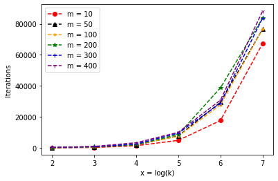
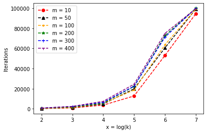
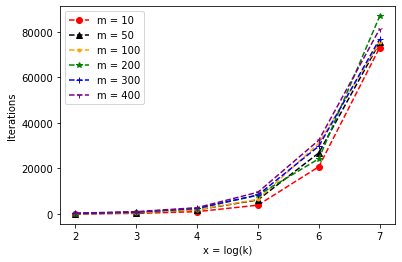
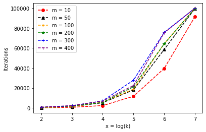
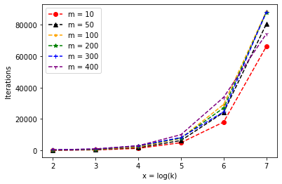
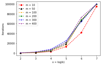
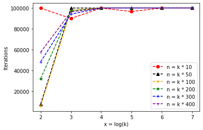
For each constructed instance of CCMSP-1, we execute each of the two algorithms on it for 30 times and take the average of the iteration numbers required for the 30 executions to solve it. However, for some instances, some executions of the algorithm cannot solve them within $10^{5}$ iterations. Under the case, we set $10^{5}$ as the iteration number that the algorithm requires to solve it. Taking into account the randomness of the experimental performance of the two algorithms, by Fig. 7-7 we find that: (1). The value of the co-variance has little influence on the performance of the two algorithms for the instances of CCMSP-1, so do the extra constraints considered in CCMSP-$2^{+}$ and CCMSP-$2^{-}$; (2). For each constructed instance of CCMSP-1, the averaged iteration number of the (1+1) EA for solving it is always larger than that of RLS, coinciding with the obtained theoretical performance of the two algorithms for CCMSP-1; and (3). The six curves increase exponentially with $\log k$, coinciding with the obtained theoretical performance of the two algorithms for CCMSP-1. Remark that for Fig. 7, 7 and 7, the slopes of some curves in region $[6,7]$ decrease compared to that in region $[5,6]$, as the (1+1) EA cannot solve these instances within $10^{5}$ iterations so that $10^{5}$ is set as the iteration number that the algorithm requires to solve them. The real slopes should be larger than that depicted in region $[6,7]$ of Fig. 7, 7 and 7.

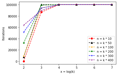
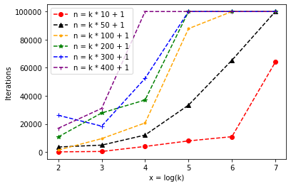
CCMSP-$2^{+}$. We separately investigate the experimental performance of RLS for CCMSP-$2^{+}$-Even and CCMSP-$2^{+}$-Odd. Because of the extra constraint considered in CCMSP-$2^{+}$, we consider the three setting approaches of the covariance $c\in\{10^{-7},10^{-8},10^{-9}\}$. The number of jobs considered in each instance is $n\in\{k*10,k*50,k*100,k*200,k*300,k*400\}$ (recall that $k\in\{2^{2},2^{3},2^{4},2^{5},2^{6},2^{7}\}$). That is, for each instance constructed for CCMSP-$2^{+}$-Even, it has a parameter-triple $(k,n,c)$. For each specific parameter-triple $(k,n,c)$, each $m_{i}$ ($1\leq i\leq k$) is set in order as follows: If $1\leq i\leq k-1$ then $m_{i}=f+g$, where $f=\lceil(n-\sum_{j=1}^{i-1}m_{i})/(k+1-i)\rceil$ and $g$ is an integer chosen from the range $[-\lceil f/2\rceil,\lceil f/2\rceil]$ uniformly at random; otherwise, $m_{k}=n-\sum_{j=1}^{k-1}m_{i}$. Therefore, there are totally 108 instances totally constructed for CCMSP-$2^{+}$-Even. To compare the experimental performance of RLS for CCMSP-$2^{+}$-Even and CCMSP-$2^{+}$-Odd, for each one $I$ of the 108 instances constructed above for CCMSP-$2^{+}$-Even, an extra job is added into a group uniformly at random such that an instance $I^{\prime}$ of CCMSP-$2^{+}$-Odd is constructed. That is, there are 108 instances totally constructed for CCMSP-$2^{+}$-Odd, and each instance $I^{\prime}$ of CCMSP-$2^{+}$-Odd has an extra job compared to the corresponding instance $I$ of CCMSP-$2^{+}$-Even.

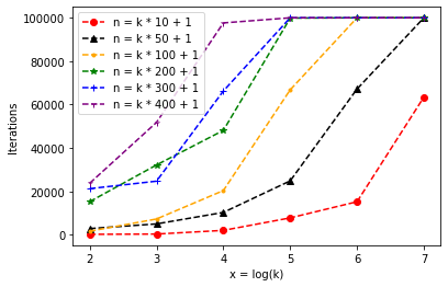
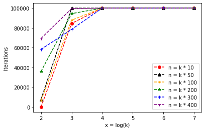
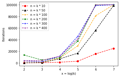
Remark that for each constructed instance of CCMSP-$2^{+}$-Even, RLS would stop once a solution satisfying the conditions given in Theorem 13 is obtained (not optimal). However, by Fig. 13, 13 and  13, almost all instances of CCMSP-$2^{+}$-Even cannot be solved by RLS within $10^{5}$ iterations if $k\geq 2^{3}$. In comparison, the experimental performance of RLS for the instances of CCMSP-$2^{+}$-Odd to obtain the optimal solutions, given in Fig. 13, 13 and 13, is much better, coinciding with the obtained theoretical performance of RLS for CCMSP-$2^{+}$.

Specifically, for the setting $c=10^{-7}$, the makespan of the obtained solutions for the corresponding 36 instances of CCMSP-$2^{+}$-Even and the 36 ones of CCMSP-$2^{+}$-Odd are listed in Table 1. It is necessary to point out that each instance $I^{\prime}$ of CCMSP-$2^{+}$-Odd has an extra job compared to the corresponding instance $I$ of CCMSP-$2^{+}$-Even, thus the makespan of the optimal solution for $I^{\prime}$ is at least 100 more than that of $I$, taking into account the expected runtime $a=100$ of the extra job, and the resulting variance and covariance. However, as mentioned before, the obtained solution for $I^{\prime}$ is not optimal but the one for $I$ is, thus the gap between the two makespan is around 100 (i.e., the gap may be larger or less than 100).

	$k=2^{2}$		$k=2^{3}$		$k=2^{4}$		$k=2^{5}$		$k=2^{6}$		$k=2^{7}$
	Even	Odd	Even	Odd	Even	Odd	Even	Odd	Even	Odd	Even	Odd
$n=k*10\ /\ k*10+1$	2,001.949,4	2,101.997,5	4,002.756,9	4,102.791,1	8,003.898,9	8,103.923,1	16,005.514,3	16,105.530,9	32,007.799,2	32,107.809,8	64,011.032,6	64,111.036,1
$n=k*50\ /\ k*50+1$	10,004.359,7	10,104.381,2	20,006.165,6	20,106.180,6	40,008.720,5	40,108.729,8	80,012.335,7	80,112.338,1	160,017.453,9	160,117.443,2	320,024.711,8	320,124.664,7
$n=k*100\ /\ k*100+1$	20,006.166,5	20,106.181,3	40,008.720,9	40,108.730,9	80,012.335,6	80,112.339,6	160,017.453,8	160,117.445,5	320,024.713,6	320,124.667,8	640,035.015,9	640,134.886
$n=k*200\ /\ k*200+1$	40,008.724,5	40,108.733,1	80,012.337,9	80,112.342,7	160,017.453,4	160,117.449,9	320,024.715,7	320,124.674,2	640,035.019,3	640,134.894,6	1,280,049.693	1,280,149.384
$n=k*300\ /\ k*300+1$	60,010.688,2	60,110.694,1	120,015.115,3	120,115.117,2	240,021.389,9	240,121.374,8	480,030.293,7	480,130.225,6	960,042.980,6	960,142.758,5	1,920,061.155	1,920,160.615
$n=k*400\ /\ k*400+1$	80,012.346,4	80,112.348,8	160,017.460,7	160,117.459,4	320,024.712	320,124.686,3	640,035.024,7	640,134.910,6	1,280,049.759	1,280,149.414	2,560,070.952	2,560,170.201

Table 1: The experimental results about the makespan for the 36 instances of CCMSP-$2^{+}$-Even and the 36 ones of CCMSP-$2^{+}$-Odd with $c=10^{-7}$.

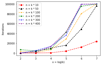
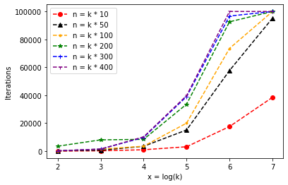
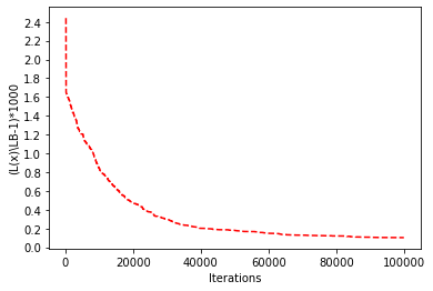
CCMSP-$2^{-}$. To meet the extra constraint considered in CCMSP-$2^{-}$, we consider the three setting approaches of the covariance $c\in\{10^{20},10^{25},10^{30}\}$. The way to construct the instances of CCMSP-$2^{-}$ is the same as that of CCMSP-$2^{+}$-Even, i.e., there are totally 108 instances constructed as well. Remark that for each constructed instance of CCMSP-$2^{-}$, RLS stops once a local optimal solution satisfying the conditions given in Theorem 15 is obtained (not optimal). By Fig. 13,  17 and 17, we have that if the value of $c$ is large enough, then its influence on the performance of the algorithm is little. Specifically, the curves given in the three figures are almost the same if $k\geq 2^{4}$. Besides, we also study the optimization process specified by an execution of RLS on an instance of CCMSP-$2^{-}$ with $c=10^{20}$, $k=2^{7}$ and $n=k*300$ (recall that $n$ is even), which is given in Fig. 17. Note that the execution would not stop unless the iteration number reaches $10^{5}$, and the vertical coordinate of Fig. 17 is $(\frac{L(x)}{LB}-1)*1000$, where $LB=\sqrt{\frac{1-\gamma}{\gamma}\frac{c}{4}\sum_{i\in S}m_{i}(m_{i}-2)}$ is the lower bound of $L(x^{*})$ of the optimal solution $x^{*}$ (we use the lower bound $LB$ to approximately replace $L(x^{*})$ as it is computationally expensive to get $L(x^{*})$, and $\frac{L(x)}{LB}$ is larger than the real approximation ratio). We find that the optimization speed is really fast at the early stage and the $y$-value is improved to 1.5 within the first 150 iterations, then the optimization speed gradually declines, and finally the $y$-value approaches 0.2 when the iteration number reaches $10^{5}$.

Figure 8: RLS for CCMSP-$2^{+}$-Even with $c=10^{-7}$.

Figure 9: RLS for CCMSP-$2^{+}$-Odd with $c=10^{-7}$.

Figure 10: RLS for CCMSP-$2^{+}$-Even with $c=10^{-8}$.

Figure 11: RLS for CCMSP-$2^{+}$-Odd with $c=10^{-8}$.

Figure 12: RLS for CCMSP-$2^{+}$-Even with $c=10^{-9}$.

Figure 13: RLS for CCMSP-$2^{+}$-Odd with $c=10^{-9}$.

Figure 14: RLS for CCMSP-$2^{-}$ with $c=10^{20}$.

Figure 15: RLS for CCMSP-$2^{-}$ with $c=10^{25}$.

Figure 16: RLS for CCMSP-$2^{-}$ with $c=10^{30}$.

Figure 17: The optimization process of RLS on an instance of CCMSP-$2^{-}$ with $c=10^{20}$, $k=2^{7}$ and $n=k*300$.

7 Conclusion

The paper studied a chance-constrained version of the Makespan Scheduling problem and investigated the performance of RLS and the (1+1) EA for it. More specifically, the paper studied three simple variants of the problem (namely, CCMSP-1, CCMSP-2⁺ and CCMSP-2^-) and obtained a series of results: CCMSP-1 was shown to be polynomial-time solvable by giving the expected runtime of RLS and the (1+1) EA (i.e., $O(n^{2}/m=O(kn))$ and $O((k+m)n^{2})$, respectively) to obtain an optimal solution to the given instance of CCMP-1; CCMSP-2⁺ was shown to be NP-hard by reducing the Two-way Balanced Partition problem to it, any instance of CCMSP-2⁺ that considers odd many jobs was shown to be polynomial-time solvable in surprise by giving the expected runtime of RLS (i.e., $O(\sqrt{k}n^{3})$) to obtain an optimal solution to it, and the properties and approximation ratio of the local optimal solution obtained by RLS for any instance of CCMSP-2⁺ that considers even many jobs were given; CCMSP-2^- was shown to be NP-hard as well, and the discussion for the approximation ratio 2 of the local optimal solution obtained by RLS was given. Related experimental results were found to coincide with these theoretical results.

It is necessary to point out that the study of RLS and the (1+1) EA for CCMSP given in the paper, compared to that for MSP given in the previous related literatures, is not just considering a new surrogate of the makespan induced by One-sided Chebyshev’s Inequality. It can be found that the value of the surrogate is also up to the variances among the jobs of the same group assigned to the same machine. Thus we have to not only consider the expected processing time and variance of each job, but also the covariances. In some way, the covariances can be treated as weights on the jobs, but they do not stay the same and dynamically change with the number of jobs of the same group assigned to the same machine. To our best knowledge, except the literature (Xie et al.,, 2019), there is no one in the area of theoretical study of EA, in which the weights on the bits are non-linear changed with the values of its neighborhood bits. Thus from this perspective, our study and the one given in (Xie et al.,, 2019) are the stepping stone to the new research area.

Future work on the other variants of the Chance-constrained Makespan Scheduling problem would be interesting, e.g., the variant of CCMSP-1 in which the covariance has two optional values, and the one of CCMSP in which everything is unknown except the loads on the two machines. Additionally, studying the chance-constrained version of other classical combinatorial optimization problems is also meaningful. These related results would further advance and broaden the understanding of evolutionary algorithms.

8 Acknowledgements

This work has been supported by the National Natural Science Foundation of China under Grant 62072476, the Open Project of Xiangjiang Laboratory under Grants 22XJ03005 and 22XJ02002, the Hunan Provincial Natural Science Foundation of China under Grants 2021JJ40791 and 2020JJ4949, and the Australian Research Council (ARC) through grant FT200100536.

References

- Assimi et al., (2020) Assimi, H., Harper, O., Xie, Y., Neumann, A., and Neumann, F. (2020). Evolutionary bi-objective optimization for the dynamic chance-constrained knapsack problem based on tail bound objectives. In Proceedings of the 24th European Conference on Artificial Intelligence (ECAI), pages 307–314.
- Blazewicz et al., (1983) Blazewicz, J., Lenstra, J., and Kan, A. (1983). Scheduling subject to resource constraints: Classification and complexity. Discrete Applied Mathematics, 5(1):11–24.
- Charnes and Cooper, (1959) Charnes, A. and Cooper, W. W. (1959). Chance-constrained programming. Management science, 6(1):73–79.
- Corus et al., (2013) Corus, D., Lehre, P. K., and Neumann, F. (2013). The generalized minimum spanning tree problem: A parameterized complexity analysis of bi-level optimisation. In Proceedings of the Genetic and Evolutionary Computation Conference (GECCO), pages 519–526. ACM.
- Doerr et al., (2020) Doerr, B., Doerr, C., Neumann, A., Neumann, F., and Sutton, A. (2020). Optimization of chance-constrained submodular functions. In Proceedings of the AAAI Conference on Artificial Intelligence, volume 34, pages 1460–1467. ACM.
- Doerr et al., (2017) Doerr, B., Le, H. P., Makhmara, R., and Nguyen, T. D. (2017). Fast genetic algorithms. In Proceedings of the genetic and evolutionary computation conference, pages 777–784.
- Friedrich et al., (2009) Friedrich, T., He, J., Hebbinghaus, N., Neumann, F., and Witt, C. (2009). Analyses of simple hybrid algorithms for the vertex cover problem. Evolutionary Computation, 17(1):3–19.
- Friedrich et al., (2010) Friedrich, T., He, J., Hebbinghaus, N., Neumann, F., and Witt, C. (2010). Approximating covering problems by randomized search heuristics using multi-objective models. Evolutionary Computation, 18(4):617–633.
- Friedrich et al., (2020) Friedrich, T., Kötzing, T., Lagodzinski, J. G., Neumann, F., and Schirneck, M. (2020). Analysis of the (1+1) EA on subclasses of linear functions under uniform and linear constraints. Theoretical Computer Science, 832:3–19.
- Graham, (1966) Graham, R. L. (1966). Bounds for certain multiprocessing anomalies. Bell system technical journal, 45(9):1563–1581.
- Gunia, (2005) Gunia, C. (2005). On the analysis of the approximation capability of simple evolutionary algorithms for scheduling problems. In Proceedings of the Genetic and Evolutionary Computation Conference (GECCO), pages 571–578. ACM.
- Hayes, (2002) Hayes, B. (2002). Computing science: The easiest hard problem. American Scientist, 90(2):113–117.
- He et al., (2014) He, J., Mitavskiy, B., and Zhou, Y. (2014). A theoretical assessment of solution quality in evolutionary algorithms for the knapsack problem. In Proceedings of the IEEE Congress on Evolutionary Computation (CEC), pages 141–148. IEEE.
- He et al., (2015) He, J., Wang, Y., and Zhou, Y. (2015). Analysis of solution quality of a multiobjective optimization-based evolutionary algorithm for knapsack problem. In Proceedings of the European Conference on Evolutionary Computation in Combinatorial Optimization (EvoCOP), pages 74–85. Springer.
- He and Yao, (2004) He, J. and Yao, X. (2004). A study of drift analysis for estimating computation time of evolutionary algorithms. Natural Computing, 3:21–35.
- Hochbaum and Shmoys, (1987) Hochbaum, D. S. and Shmoys, D. B. (1987). Using dual approximation algorithms for scheduling problems theoretical and practical results. Journal of the ACM (JACM), 34(1):144–162.
- Iwamura and Liu, (1996) Iwamura, K. and Liu, B. (1996). A genetic algorithm for chance constrained programming. Journal of Information and Optimization Sciences, 17(2):409–422.
- Jansen et al., (2013) Jansen, T., Oliveto, P. S., and Zarges, C. (2013). Approximating vertex cover using edge-based representations. In Proceedings of the Workshop on Foundations of Genetic Algorithms (FOGA), pages 87–96. ACM.
- Kratsch et al., (2010) Kratsch, S., Lehre, P. K., Neumann, F., and Oliveto, P. S. (2010). Fixed parameter evolutionary algorithms and maximum leaf spanning trees: A matter of mutation. In Proceedings of the Conference on Parallel Problem Solving from Nature (PPSN), pages 204–213. Springer.
- Kratsch and Neumann, (2013) Kratsch, S. and Neumann, F. (2013). Fixed-parameter evolutionary algorithms and the vertex cover problem. Algorithmica, 65(4):754–771.
- Kumar and Banerjee, (2005) Kumar, R. and Banerjee, N. (2005). Running time analysis of a multiobjective evolutionary algorithm on simple and hard problems. In Proceedings of the Workshop on Foundations of Genetic Algorithms (FOGA), pages 112–131. ACM.
- Lissovoi and Witt, (2017) Lissovoi, A. and Witt, C. (2017). A runtime analysis of parallel evolutionary algorithms in dynamic optimization. Algorithmica, 78(2):641–659.
- Miller and Wagner, (1965) Miller, B. L. and Wagner, H. M. (1965). Chance constrained programming with joint constraints. Operations Research, 13(6):930–945.
- Neumann and Neumann, (2020) Neumann, A. and Neumann, F. (2020). Optimising monotone chance-constrained submodular functions using evolutionary multi-objective algorithms. In Proceedings of the 16th International Conference on Parallel Problem Solving from Nature (PPSN), pages 404–417. Springer.
- Neumann et al., (2022) Neumann, A., Xie, Y., and Neumann, F. (2022). Evolutionary algorithms for limiting the effect of uncertainty for the knapsack problem with stochastic profits. In Proceedings of the Conference on Parallel Problem Solving from Nature (PPSN), pages 294–307. Springer.
- Neumann et al., (2020) Neumann, F., Pourhassan, M., and Roostapour, V. (2020). Analysis of evolutionary algorithms in dynamic and stochastic environments, pages 323–357. Springer International Publishing, Cham.
- Neumann and Sutton, (2018) Neumann, F. and Sutton, A. M. (2018). Runtime analysis of evolutionary algorithms for the knapsack problem with favorably correlated weights. In Proceedings of the Conference on Parallel Problem Solving from Nature (PPSN), pages 141–152. Springer.
- Neumann and Sutton, (2019) Neumann, F. and Sutton, A. M. (2019). Runtime analysis of the (1+1) evolutionary algorithm for the chance-constrained knapsack problem. In Proceedings of the Workshop on on Foundations of Genetic Algorithms (FOGA), pages 147–153. ACM.
- Neumann and Wegener, (2006) Neumann, F. and Wegener, I. (2006). Minimum spanning trees made easier via multi-objective optimization. Natural Computing, 5:305–319.
- Neumann and Wegener, (2007) Neumann, F. and Wegener, I. (2007). Randomized local search, evolutionary algorithms, and the minimum spanning tree problem. Theoretical Computer Science, 378(1):32–40.
- Neumann and Witt, (2015) Neumann, F. and Witt, C. (2015). On the runtime of randomized local search and simple evolutionary algorithms for dynamic makespan scheduling. In Proceedings of the 24th International Joint Conference on Artificial Intelligence (IJCAI), pages 3742–3748. ACM.
- Numata, (1988) Numata, K. (1988). Approximate and exact algorithms for scheduling independent tasks on unrelated processors. Journal of the Operations Research Society of Japan, 31(1):61–81.
- Oliveto et al., (2008) Oliveto, P. S., He, J., and Yao, X. (2008). Analysis of population-based evolutionary algorithms for the vertex cover problem. In Proceedings of the IEEE Congress on Evolutionary Computation (IEEE World Congress on Computational Intelligence), pages 1563–1570. IEEE.
- Oliveto et al., (2009) Oliveto, P. S., He, J., and Yao, X. (2009). Analysis of the (1+1) EA for finding approximate solutions to vertex cover problems. IEEE Transactions on Evolutionary Computation, 13(5):1006–1029.
- Poojari and Varghese, (2008) Poojari, C. A. and Varghese, B. (2008). Genetic algorithm based technique for solving chance constrained problems. European journal of operational research, 185(3):1128–1154.
- Pourhassan et al., (2017) Pourhassan, M., Friedrich, T., and Neumann, F. (2017). On the use of the dual formulation for minimum weighted vertex cover in evolutionary algorithms. In Proceedings of the Workshop on Foundations of Genetic Algorithms (FOGA), pages 37–44. ACM.
- Pourhassan et al., (2015) Pourhassan, M., Gao, W., and Neumann, F. (2015). Maintaining 2-approximations for the dynamic vertex cover problem using evolutionary algorithms. In Proceedings of the Genetic and Evolutionary Computation Conference (GECCO), pages 513–518. ACM.
- Pourhassan et al., (2016) Pourhassan, M., Shi, F., and Neumann, F. (2016). Parameterized analysis of multi-objective evolutionary algorithms and the weighted vertex cover problem. In Proceedings of the Conference on Parallel Problem Solving from Nature (PPSN), pages 729–739. Springer.
- Roostapour et al., (2018) Roostapour, V., Neumann, A., and Neumann, F. (2018). On the performance of baseline evolutionary algorithms on the dynamic knapsack problem. In Proceedings of the Conference on Parallel Problem Solving from Nature (PPSN), pages 158–169. Springer.
- Roostapour et al., (2022) Roostapour, V., Neumann, A., Neumann, F., and Friedrich, T. (2022). Pareto optimization for subset selection with dynamic cost constraints. Artificial Intelligence, 302:103597.
- Sahni, (1976) Sahni, S. K. (1976). Algorithms for scheduling independent tasks. Journal of the ACM (JACM), 23(1):116–127.
- Shi et al., (2021) Shi, F., Neumann, F., and Wang, J. (2021). Runtime performances of randomized search heuristics for the dynamic weighted vertex cover problem. Algorithmica, 83(4):906–939.
- Shi et al., (2019) Shi, F., Schirneck, M., Friedrich, T., Kötzing, T., and Neumann, F. (2019). Reoptimization time analysis of evolutionary algorithms on linear functions under dynamic uniform constraints. Algorithmica, 81(2):828–857.
- Shi et al., (2022) Shi, F., Yan, X., and Neumann, F. (2022). Runtime analysis of simple evolutionary algorithms for the chance-constrained makespan scheduling problem. In Proceedings of the Conference on Parallel Problem Solving from Nature (PPSN), pages 526–541. Springer.
- Sutton and Neumann, (2012) Sutton, A. M. and Neumann, F. (2012). A parameterized runtime analysis of simple evolutionary algorithms for makespan scheduling. In Proceedings of the 12th International Conference on Parallel Problem Solving from Nature (PPSN), pages 52–61. Springer.
- Vahid et al., (2020) Vahid, R., Jakob, B., and Neumann, F. (2020). Runtime analysis of evolutionary algorithms with biased mutation for the multi-objective minimum spanning tree problem. In Proceedings of the Genetic and Evolutionary Computation Conference (GECCO), pages 551–559. ACM.
- Witt, (2005) Witt, C. (2005). Worst-case and average-case approximations by simple randomized search heuristics. In Annual Symposium on Theoretical Aspects of Computer Science, pages 44–56. Springer.
- Witt, (2014) Witt, C. (2014). Revised analysis of the (1+1) EA for the minimum spanning tree problem. In Proceedings of the Genetic and Evolutionary Computation Conference (GECCO), pages 509–516. ACM.
- Wu et al., (2016) Wu, J., Polyakovskiy, S., and Neumann, F. (2016). On the impact of the renting rate for the unconstrained nonlinear knapsack problem. In Proceedings of the Genetic and Evolutionary Computation Conference (GECCO), pages 413–419. ACM.
- Xie et al., (2019) Xie, Y., Harper, O., Assimi, H., Neumann, A., and Neumann, F. (2019). Evolutionary algorithms for the chance-constrained knapsack problem. In Proceedings of the Genetic and Evolutionary Computation Conference (GECCO), pages 338–346. ACM.
- Xie et al., (2020) Xie, Y., Neumann, A., and Neumann, F. (2020). Specific single- and multi-objective evolutionary algorithms for the chance-constrained knapsack problem. In Proceedings of the Genetic and Evolutionary Computation Conference (GECCO), pages 271–279. ACM.
- Xie et al., (2021) Xie, Y., Neumann, A., Neumann, F., and Sutton, A. M. (2021). Runtime analysis of RLS and the (1+ 1) EA for the chance-constrained knapsack problem with correlated uniform weights. In Proceedings of the Genetic and Evolutionary Computation Conference (GECCO), pages 1187–1194. ACM.
- Yu et al., (2012) Yu, Y., Yao, X., and Zhou, Z.-H. (2012). On the approximation ability of evolutionary optimization with application to minimum set cover. Artificial Intelligence, 180:20–33.