Does peer-reviewed theory help predict the cross-section of stock returns? 00footnotetext: First posted to arxiv.org: December 2022. E-mails: andrew.y.chen@frb.gov, Alejandro.Lopez-Lira@warrington.ufl.edu, tom.zimmermann@uni-koeln.de. Earlier versions of this paper relied on data provided by Sterling Yan and Lingling Zheng, to whom we are grateful. We thank Alec Erb for excellent research assistance. For helpful comments, we thank Svetlana Bryzgalova, Leland Bybee (discussant), Charlie Clarke, Mike Cooper, Yufeng Han (discussant), Albert Menkveld, Ben Knox, Emilio Osambela, Dino Palazzo, Matt Ringgenberg, Yinan Su (discussant), Lingling Zheng, and seminar participants at Auburn University, Baruch College, Emory University, the Fed Board, Louisiana State, University of Utah, University of Wisconsin-Milwaukee, and Virginia Tech. The views in this paper are not necessarily those of the Federal Reserve Board or the Federal Reserve System.
Abstract
We compare four groups of cross-sectional return predictors: (1) published with a risk-based explanation, (2) published with a mispricing explanation, (3) published with uncertain origins, and (4) naively data-mined from accounting variables. For all groups, predictability decays by 50% post-sample, showing theory does not help predict returns above naive backtesting. Data-mined predictors display features of published predictors including the rise in returns as in-sample periods end, the speed of post-sample decay, and themes from the literature like investment, issuance, and accruals. Our results imply peer-review systematically mislabels mispricing as risk, though only 18% of predictors are attributed to risk.
1 Introduction
Since at least [34], asset pricing researchers have been worried about data mining bias. These worries permeate the field. In fact, the terms “data mining” (searching through data for patterns) and “data mining bias” (the bias that comes from ignoring the search) are used interchangeably (e.g. [31]).
The consensus solution for data mining bias is the use of economic theory. In his influential textbook, [18] writes: “[t]he best hope for finding pricing factors that are robust out of sample… …is to try to understand the fundamental macroeconomic sources of risk.” [31] go further and assert that not only is theory our best hope, but that “[e]conomic theories are based on a few economic principles and, as a result, there is less room for data mining.” This idea that using theory protects against data mining bias is also found throughout Harvey’s \citeyearparharvey2017presidential AFA Presidential Address, almost 50 years after [34].
We question this consensus. With modern computing power, a talented theorist can justify nearly any empirical pattern ([47]; [40]). Peer review should restrict published theories to those based on risk or some other real-world fundamentals. However, the effectiveness of peer review is not known. Indeed, none of the aforementioned writings provides an empirical test of whether theory does protect against data mining bias. Our paper fills this gap.
Our test answers the following hypothetical question: suppose someone tells you he found a cross-sectional return predictor with a t-stat of 3.0 and a long-short mean return of 100 bps per month in a historical sample. How would your inference about the expected post-sample return change if the predictor is:
-
1.
Supported by a publishable risk-based explanation,
-
2.
Supported by a publishable mispricing explanation,
-
3.
Of uncertain origins, but still publishable,
-
4.
Or mined from accounting data?
In other words, how should your expectation of future predictability depend on the origins of predictability? If economic theory protects against data mining bias and post-sample decay, then the origin matters a lot.
To answer this question, we assign 199 published cross-sectional stock return predictors to “risk,” “mispricing,” or “agnostic,” groups based on the explanation for predictability in the original papers. We create a fourth group of predictors by mining accounting data for t-stats and mean returns that are similar to those of published predictors (using the original papers’ sample periods). Finally, we measure the post-sample return within each group.
Our main finding is that the post-sample return depends little on the origins of predictability. Regardless of whether a predictor has a publishable risk-based explanation, a mispricing explanation, or is publishable without a clear explanation, the post-sample return is about 50% smaller than the in-sample return. We strongly reject the hypothesis that risk-based theory prevents post-sample decay (-value 0.1%).
It does not even matter if the predictor is purely data mined. Our data mining procedure is best described as naive back-testing. Inspired by [52], we begin with 242 accounting variables, and then form 29,000 trading strategies by (1) dividing one variable by another or (2) taking first differences and then dividing. The only restriction is that we require the denominators to be variables that are positive for more than 25% of firms in 1963. We search these 29,000 strategies for t-stats and mean returns that are similar to published predictors, using the published sample periods. Despite the complete lack of economics in this procedure, it leads to post-sample returns that are just a touch smaller than the published counterparts.
To put these results in perspective, we provide a statistical model for why economic theory should protect against data mining bias. The model generalizes [11]’s empirical Bayes framework (see also [15]; [35]) to allow for different predictor origins. It shows that theory leads to less out-of-sample decay compared to data mining if theoretically justified predictors have higher and more stable expected returns, holding fixed in-sample summary statistics. In other words, theory helps predict returns if it provides information about expected returns. Our empirical results imply, unfortunately, that theory does not provide such information.
Though these findings are negative for economic theory, they are positive for data mining. As shown by [52], data mining uncovers true out-of-sample predictability, a result replicated by our paper as well as Goto and Yamada (2022). While data mining can result in a bias, this bias can be removed using empirical Bayes and related methods ([20, 11, 35]). Indeed, fields like protein folding and language modeling have been revolutionized by atheoretical searches through vast amounts of data ([36]; [54]). And while data mined results say little about the underlying economics, they can provide the empirical foundation for the next generation of theory.
Our second main result is that peer-reviewed returns behave quite similarly to data-mined returns in event time, where the event is defined as the end of the original paper’s in-sample period. Both published and data-mined returns increase in the years just before the original samples end, fall significantly in the first five years out-of-sample, and flatten out for years 10-15, before dipping temporarily around the 18th year out-of-sample. Moreover, data mining uncovers themes from the academic literature like investment, issuance, and accruals. These patterns are not extracted from the matching process—the match is formed on only two in-sample summary statistics. Instead, these patterns emerge from the data itself: historical waves of finance publications and return predictability jointly produce the same patterns of portfolio returns, whether the portfolios come from peer review or data mining. It’s as if the finance academics are just mining accounting data for return predictability, and then decorating the results with stories about risk and psychology.
Our last main result is that there is a striking consensus about the origins of cross-sectional predictability in peer-reviewed papers. Among the 199 published predictors we examine, only 18% are attributed to risk by the peer review process. 59% are attributed to mispricing, and 23% have uncertain origins.
This consensus is a positive sign regarding the peer review process. The fact that risk-based predictors decay post-sample implies that peer review either mislabels mispricing as risk or finds unstable risk factors that disappear over time. Fortunately, these errors are relatively uncommon, and represent a relatively small “false discovery rate.”
A more negative view of the peer review process, however, comes from the fact that recent reviews are typically agnostic about risk vs mispricing ([2]; [53]). Given the strong consensus found from reading the individual papers, this agnosticism suggests that the battle between risk-based and behavioral finance has led to an unwillingness to engage in open debate. We hope our paper provides the impetus to re-open discussion of these core issues.
We use alternative data mining methods and theory measurements to pin down the mechanism. We find the key to generating research-like returns from data mining is to simply screen accounting signals for in-sample statistical significance. Mining accounting data seems to be important as mining tickers (a la [29]) leads to out-of-sample returns close to zero. Excluding correlated returns has little effect on our results. We also find robustness to using factor model measures of risk and to focusing on quantitative equilibrium models.
Replication code and the returns of 29,000 data-mined strategies can be found via https://github.com/chenandrewy/flex-mining. The predictor categorizations, as well as the excerpts that lead to the categorizations, are found at https://github.com/chenandrewy/flex-mining/blob/main/DataInput/SignalsTheoryChecked.csv.
The remainder of this section reviews literature. Section 2 formalizes “Cochrane’s Hope”: the idea that theory can help find robust stock return patterns. Section 3 examines how post-sample returns depend on peer-reviewed theoretical origins. Section 4 compares published and data-mined strategies. Section 5 examines alternative specifications. Section 6 concludes.
1.1 Related Literature
We add to the literature on data mining in return predictability. [39] provides an early theoretical examination; Sullivan, Timmermann, and White (\citeyearsullivan1999data, \citeyearsullivan2001dangers) study bias in market timing strategies; and [41] measure data-mining bias in published predictors. But to our knowledge, it was not until [52] that anyone systematically mined accounting data for cross-sectional predictors.
Surprisingly, Yan and Zheng find that find data mining leads to “many” predictors that cannot be accounted for by luck using a bootstrap procedure ([24]). Moreover, they find data mining generates substantial out-of-sample alphas. We replicate and extend Yan and Zheng’s results. While Yan and Zheng’s data-mining strategies are inspired by functional forms used in the literature and are rescaled using economic intuition, our data-mining process is arguably free of economics. We show that not only does economics-free data mining generate substantial out-of-sample performance, but this out-of-sample performance is just as strong as the performance found through the peer-review process.
These results provide clarity to the conflicting evidence on accounting-based data mining. Using FDR methods, [30] find evidence inconsistent with Yan and Zheng’s results, while [9] finds evidence in support. Since FDR methods are complex and can be easily misinterpreted ([12]), we focus exclusively on out-of-sample tests, which are well-understood and have straightforward interpretations. Our findings support not only Yan and Zheng’s conclusion of “many” true predictors, but that the number of true predictors is in the thousands. In contemporaneous work, [27] also find support for this conclusion.
Our results provide an alternative perspective on the question of how investors interact with academic research. [41] argue that investors learn from academic publications, as evidenced by the systematic decline in return predictability after publication that cannot be explained by data mining bias (see also [11, 35]). This story is also seen in the trades of short sellers and hedge funds ([41, 8, 42]). Our findings suggest that both academic research and investors are responding to the same fundamentals: the appearance of statistically significant return predictability in accounting data. Once return predictability appears, it is diminished through investor learning, and academics scientifically document a select subset of these phenomena.
2 Why Should Theory Help?
This section provides a meta-theory for why economic theory should help predict returns out-of-sample. The model builds on [11] (see also [35]).
2.1 A Model of Data-Mining and Decay
The return of strategy in month depends on whether it is in-sample () or out-of sample ():
| (1) |
where is the expected return in-sample, is the change in expected returns post-sample, is the length of the in-sample period, and is a zero mean residual. is the in-sample mean and is the post-sample mean, where is the length of the post-sample period. and are the corresponding sample means of the residuals. is unpredictable using information known before time .
Let represent the strategies one can make from mining some dataset. For example, may consist of the strategies one can make from 240 accounting variables by dividing one variable by another variable, and then forming long-short deciles. We assume is not constructed using out-of-sample information, and so
| (2) |
Data mining does not necessarily lead to a bias. For example, if is selected randomly from and is selected without using in-sample information, then the post-sample decay corresponds entirely to a decline in expected returns
| (3) |
since the residuals have zero mean.
In practice, data mining is not random. Instead, it involves selecting the best strategies, say , where is a threshold that may depend on . As a result, practical data mining leads to a bias:
| (4) |
where the term disappears due to Equation (2). The bias is embodied in the term, which is in general positive. Intuitively, selecting for large also selects for large (see Equation (1)).111For example, in a Gaussian setting this term is positive if . See Equation (18) and Equation (8) of [11]. This selection is the essence of data mining bias, publication bias, and related problems ([11, 12]). Data mining often involves switching the long and short legs depending on the sign of , which leads to more complex expressions, but the intuition remains the same (see Appendix A.1).
Thus, there are two distinct problems that lead to post-sample decay: (1) a decline in expected returns and (2) data mining bias. Applying economic theory should help with both problems.
2.2 Why Applying Economic Theory Should Help
Applying economic theory amounts to studying strategies from a set rather than . represents consistency with some class of economic theory (e.g. risk-based theories). We assume that is also selected using only in-sample information, and thus , as in Equation (2). Critically, the distribution of may differ from the distribution of , and thus theory may be helpful for finding expected returns.
Formally, we define helpful theories as follows:
Definition 1.
is helpful relative to if
| (5) | ||||
| (6) |
where .
Equation (5) says that helpful theories should lead to higher expected returns than data mining, holding in-sample mean returns constant. This expression is perhaps the simplest way to define a helpful theory. But one can also think of this expression as saying that a helpful theory should help us differentiate fundamental equilibrium patterns () from non-equilibrium deviations ().
Equation (6) says that helpful theories should identify stable expected returns. Equilibrium is by definition a state in which return patterns are in some sense stable. This stability implies that helpful theories reduce in Equation (4), at least relative to data mining.
If Definition 1 holds, then theory leads to more less out-of-sample decay:
Proposition 1 (Cochrane’s Hope).
If is helpful compared to , then
where
The proof is in Appendix A.1.
We describe Proposition 1 as “Cochrane’s Hope” because of his discussion of “factor fishing” in Chapter 7 of his \citeyearcochrane2009asset textbook. There, he describes theory as the “best hope for finding pricing factors that are robust out of sample.” Proposition 1 provides a formal justification for this “best hope,” in the more general setting of finding out-of-sample returns.
Proposition 1 contrasts with [31], which argues that the size of relative to is important. Interestingly, the size of these sets does not appear in Proposition 1. Indeed, a helpful very well might be larger than . What matters for out-of-sample robustness is which set provides a better signal about and , not which set is smaller.
[29] argues for imposing priors based on “economic plausibility” when making inferences about . This recommendation amounts to assuming that is helpful. Instead, our study empirically tests whether is helpful, effectively making inferences about what our priors should be, much in the way empirical Bayes methods estimate prior distributions ([11]).
2.3 Data Mining Under a Factor Structure
Under some factor structures, it is easy to find an asset pricing model with a high cross-sectional ([38]). Some factor structures imply atheoretical PCA pricing models have small errors ([37]; [17]). This section examines Proposition 1 through the lens of a factor structure.
Assuming a factor structure amounts to imposing a specific form for and in Equation (1). For simplicity, consider a single factor model:
| (7) |
where is the single factor realization, is asset ’s loading on the factor, and allows for the possibility that betas decay out-of-sample.
In this case, out-of-sample decay satisfies:
| (8) |
As in Equation (4), there are two problems that lead to decay: (1) the selected strategies may have unstable betas () and (2) the selected returns are driven by sampling noise ( > 0).
Theory can help address both problems. Theory can tell us whether the measured is stable or will decay out-of-sample . It can also tell us whether sample mean returns are due to fundamental factor exposure () or lucky in-sample events ( > 0). So under a factor structure, Definition 1 is an intuitive definition of a helpful theory, and a helpful theory should reduce out-of-sample decay relative to data mining (Proposition 1).
3 Peer-Reviewed Theory and Out-of-Sample Performance
This section describes how we measure peer-reviewed theory. We also show how out-of-sample predictability varies by type of theory. Readers eager to compare theory with data mining should skip to Section 4.
3.1 Published Predictor Data
Our peer-reviewed predictors come from August 2023 release of the [13] (CZ) dataset. This dataset is built from 212 firm-level variables that were shown to predict returns cross-sectionally. It covers the vast majority of firm-level predictors that can be created from widely-available data and were published before 2016.
We drop five predictors that produce mean long-short returns of less than 15 bps per month in-sample in CZ’s replications. These predictors are rather distant from the original papers, and dropping them ensures that the decay we document accurately reflects the literature.222For example, CZ equal-weight the [26] betting against beta portfolios instead weighting by betas. CZ use CRSP age rather than the NYSE archive data used by [4]. CZ also find very small returns in simple long-short strategies for select variables shown by [32], [1], [46] to predict returns in multivariate settings. Since these predictors are rare, including them has little effect on our results.
We drop another 8 predictors that have less than 9 years of post-sample returns. Most of these predictors rely on specialized data that have been discontinued, though a few are published relatively recently. This filter makes the out-of-sample results easy to interpret. But since the median post-sample length is about 20 years, including these predictors has little effect on our results.
For measuring out-of-sample performance, we use the “original paper” version of the CZ data. These data consist of long-short portfolios constructed following the procedures in the original papers. This choice is important, as out-of-sample decay varies by the details of the trading strategy ([10]). Choosing the original implementations means that the decay we find is not due to a dispute with the peer review process about where exactly risk premiums should show up.
3.2 Measuring Peer-Reviewed Theory
To classify predictors, we read the corresponding paper and identify a passage of text that summarizes the main argument. These passages are typically taken from either the abstract, introduction, or conclusion. We then categorize each argument as “risk,” “mispricing,” or “agnostic.” Each predictor was reviewed by two of the authors to prevent errors.
These examples illustrate how we manually categorize predictors as risk, mispricing, or agnostic. Risk-to-mispricing words are counted by software and defined in Appendix A.2.
| Reference | Predictor | Example Text | Risk to |
| Mispricing | |||
| Words | |||
| Panel (a): Risk | |||
| Tuzel 2010 | Real estate holdings | Firms with high real estate holdings are more vulnerable to bad productivity shocks and hence are riskier and have higher expected returns. | 17.60 |
| Bazdresch, Belo, and Lin 2014 | Employment growth | We interpret this difference in average returns, which we refer to as the hiring return spread, as reflecting the relatively lower risk of the firms with higher hiring rates | 7.32 |
| Fama and MacBeth 1973 | CAPM beta | The pricing of common stocks reflects the attempts of risk-averse investors to hold portfolios that are "efficient" in terms of expected value and dispersion of return. | 2.31 |
| Panel (b): Mispricing | |||
| Ikenberry, Lakonishok, Vermaelen 1995 | Share repurchases | Thus, at least with respect to value stocks, the market errs in its initial response and appears to ignore much of the information conveyed through repurchase announcements | 0.05 |
| Eberhart, Maxwell, and Siddique 2004 | Unexpected R&D increase | We find consistent evidence of a mis-reaction, as manifested in the significantly positive abnormal stock returns that our sample firms’ shareholders experience following these increases. | 0.05 |
| Desai, Rajgopal, Venkatachalam 2004 | Operating Cash flows to price | CFO/P is a powerful and comprehensive measure that subsumes the mispricing attributed to all the other value-glamour proxies. | 0.05 |
| Panel (c): Agnostic | |||
| Banz 1981 | Size | To summarize, the size effect exists but it is not at all clear why it exists. | 1.93 |
| Boudoukh et al. 2007 | Net Payout Yield | We show that the apparent demise of dividend yields as a predictor is due more to mismeasurement than alternative explanations such as spurious correlation, learning, etc. | 1.00 |
| Chordia, Subra, Anshuman 2001 | Volume Variance | However, our findings do not lend themselves to an obvious explanation, so that further investigation of our results would appear to be a reasonable topic for future research. | 0.21 |
Table 1 provides representative passages for predictors in each category. Categorizing risk and mispricing predictors is straightforward. Risk passages typically discuss risk or equilibrium, though a few also emphasize market efficiency. Mispricing passages discuss mispricing or investor errors. Agnostic passages are slightly more difficult to classify. Agnostic predictors are clear when they claim agnosticism or provide arguments for both risk and mispricing. But in some cases, agnostic papers avoid discussing the theory and focus on the empirics (e.g. Boudoukh et al. 2007).
We categorize predictors into “risk,” “mispricing,” or “agnostic” based on manually reading the original papers (Table 1). “Risk Words to Mispricing Words” shows the ratio of word counts in the papers. The word list is in Appendix A.2. p05, p50, and p95 are the 5th, 50th, and 95th percentiles within each theory category.
| Source of | Num Published Predictors | Risk Words to Mispricing Words | ||||||||
| Predictability | Total | 1981-2004 | 2005-2016 | p05 | p50 | p95 | ||||
| Risk | 36 | 5 | 31 | 0.33 | 3.41 | 12.74 | ||||
| Mispricing | 117 | 48 | 69 | 0.07 | 0.22 | 1.17 | ||||
| Agnostic | 46 | 16 | 30 | 0.12 | 0.54 | 3.91 | ||||
| Any | 199 | 69 | 130 | 0.07 | 0.33 | 7.02 | ||||
Our analysis finds a remarkable consensus about the origins of cross-sectional predictability. This consensus is seen in Table 2, which counts the number of predictors in each theory category. Only 18% of cross-sectional predictors are judged by the peer review process to be due to risk. In contrast, 59% of predictors are due to mispricing. The remaining 23% of predictors are agnostic. The Appendix Table A.4 shows that finance journals more commonly find risk explanations compared to accounting journals, but they still attribute a small minority of predictors to risk.
As a check on our manual classifications, we use software to count the ratio of “risk words” to “mispricing words” in each paper. For example, we count “utility,” “maximize,” and “priced” as risk words, and “behavioral,” “optimistic,” and “sentiment” as mispricing words (see Appendix A.2 for a full list). Table 2 shows order statistics of this ratio within each manually-classified theory category. The median ratio for risk-based predictors is 3.41—that is, risk words appear 3.4 times more frequently than mispricing words. Mirroring this result, mispricing-based predictors have a median ratio of 0.22, indicating five times as many mispricing words. Overall, this simple word count supports our manual categorizations. The distribution of risk to mispricing words for risk-based predictors is far to the right of the other categories.
The word counts also support our finding that risk explains a small minority of predictors. Across all papers, the median risk-to-mispricing word ratio is 0.33, meaning that mispricing-related words are typically mentioned 3 times as frequently as risk-related words.
The consensus in Table 2 is perhaps surprising given the tone in recent reviews on empirical cross-sectional asset pricing (e.g. [2, 53]). These reviews provide a largely agnostic description of the origins of predictability, suggesting that peer review has come to a divided view, or that this topic has been too contentious to be available for open debate. Our results show that the literature favors mispricing, and that only a small minority of predictors are due to risk, as judged by the community of finance scholars.
3.3 Out-of-Sample Performance by Type of Peer-Reviewed Theory
Figure 1 shows the post-sample returns of risk-based, mispricing-based, and agnostic predictors, where the origins of predictability are judged by the peer-review process. The plot shows long-short returns in event time, where the event is the end of the original papers’ in-sample periods. We average across predictors within each month and then take the trailing 5-year average of these returns for ease of reading. Each strategy is normalized so that its mean in-sample return is 100 bps per month.
The plot shows the mean long-short returns of published predictors in event time, where the event is the end of the original sample periods. Each predictor is normalized so that its mean in-sample return is 100 bps per month. Predictors are grouped by theory category based on the arguments in the original papers (Table 1). We average returns across predictors within each month and then take the trailing 5-year average for readability. For all categories of theory, predictability decays by roughly 50% post-sample. If anything, risk-based predictors decay more than other predictors.
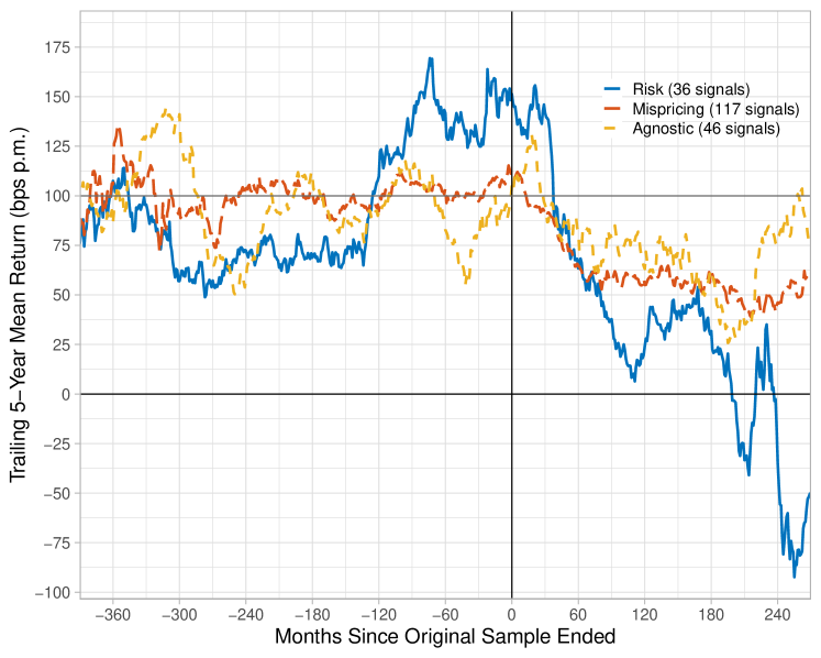
All three kinds of predictability decay by roughly 50% post-sample. These results answer, in part, the hypothetical question posed at the beginning of the paper (Section 1). It does not matter if a published predictor is justified by risk, mispricing, or lacks a definitive explanation, the expected post-sample return is similar.
Indeed, risk-based predictability seems to decay even more than mispricing-based predictability. However, this difference is unlikely to be statistically significant, due to the noisiness of 5-year mean returns, and the fact that relatively few published predictors are attributed to risk.
Table 3 examines statistical significance in a regression framework (following [41]). Specification (1) regresses monthly long-short returns on a post-sample indicator and its interaction with an indicator for risk-based theory. Returns are normalized to be 100 bps per month in-sample, so the post-sample coefficient implies that returns decay by 42 percent overall (across all theories). The interaction coefficient implies that risk-based theory leads to an additional decay of 29 percentage points, for a total decay of 71 percent.
We regress monthly long-short strategy returns on indicator variables to quantify the effects of peer-reviewed theory on predictability decay. Each strategy is normalized to have 100 bps per month returns in the original sample. “Post-Sample” is 1 if the month occurs after the predictor’s sample ends and is zero otherwise. “Post-Pub” is defined similarly. “Risk” is 1 if peer review argues for a risk-based explanation (Table 1) and 0 otherwise. “Mispricing” and “Post-2004” are defined similarly. Parentheses show standard errors clustered by month. “Null: Risk No Decay” shows the -value that tests whether risk-based returns do not decrease post-sample ((1) and (3)) or post-publication ((2) and (4)). The decay in risk-based predictors is highly statistically significant, and inconsistent with the hypothesis that risk theory uncovers stable expected returns.
| LHS: Long-Short Strategy Return (bps pm, scaled) | |||||
| RHS Variables | (1) | (2) | (3) | (4) | (5) |
| Intercept | 100.0 | 100.0 | 100.0 | 100.0 | 102.4 |
| (6.4) | (6.4) | (6.4) | (6.4) | (6.8) | |
| Post-Sample | -42.3 | -25.3 | -36.5 | -24.4 | 0.7 |
| (8.6) | (11.7) | (10.3) | (15.3) | (14.5) | |
| Post-Pub | -21.0 | -14.9 | |||
| (12.1) | (17.5) | ||||
| Post-Sample x Risk | -28.7 | -18.5 | -34.4 | -19.5 | -23.4 |
| (15.4) | (20.2) | (17.1) | (22.8) | (15.2) | |
| Post-Pub x Risk | -14.2 | -20.3 | |||
| (27.2) | (30.2) | ||||
| Post-Sample x Mispricing | -8.1 | -1.3 | |||
| (7.8) | (15.5) | ||||
| Post-Pub x Mispricing | -8.7 | ||||
| (17.5) | |||||
| Post-2004 | -59.6 | ||||
| (16.6) | |||||
| Null: Risk No Decay | 0.1% | 0.1% | 0.1% | 0.1% | 0.1% |
The additional decay of risk predictors is only marginally significant, with a standard error of 15 bps. Despite the minimum of 9 years of post-sample returns, the fact that peer-review only attributes 36 predictors to risk means that the data on this interaction is somewhat limited.
Nevertheless, there is plenty of data to show that risk-based theory fails to prevent post-sample decay. This result is shown in the row “Null: Risk No Decay,” which tests the hypothesis that the sum of the Post-Sample and Post-Sample Risk coefficients is non-negative. The test rejects this hypothesis at the 0.1% level.
Specifications (2)-(4) show robustness. Specification (2) adds a post-publication indicator, specification (3) adds an indicator for mispricing-based theory, and specification (4) adds both. All three alternative specifications arrive at risk-based predictors decaying by an additional 30 to 40 percentage points. Specification (4) implies that post-publication, being risk-based implies an additional 20 + 20 = 40 percentage points of decay, for a total decay of 24 + 15 + 40 = 79%.
Additional robustness is shown in specification (5), which controls for the idea that information technology has led to weaker predictability post-2004 ([16]). In this specification, risk-based predictors still decay more, though the magnitude is reduced. In Section 5.4, we show that decay also occurs for predictors with the highest risk words to mispricing words ratio.
4 Peer-Reviewed Theory vs Naive Data-Mining
We’ve shown that post-sample returns do not depend on the theoretical explanation for published predictors. We now compare these publication-based returns to naive data mining.
4.1 Data-Mined Trading Strategies
We generate 29,315 firm-level signals as follows. Let be one of 242 Compustat accounting variables + CRSP market equity and be one of the 65 variables that is observed and positive for 25% of firms in 1963 with matched CRSP data. We form signals by combining all combinations of ratios () and scaled first differences (). Restricting to be positive for at least a meaningful minority of stocks avoids normalizing by zero and negative numbers. This procedure would lead to signals, but we drop 2,145 signals that are redundant in “unsigned” portfolio sorts.333For the ratios where the numerator is also a valid denominator, there are only 65 choose 2 = 2,080 ratios that are distinct in the sense that there are no ratios which would lead to identical rankings if the sign was flipped.
We lag each signal by six months, and then form long-short decile strategies by sorting stocks on the lagged signals in each June. Delisting returns and other data handling methods follow [13] to ensure that the published and data-mined strategies are comparable. For further details, please see the Github repo.
In our view, this process is the simplest reasonable data mining procedure. A reasonable data mining procedure should include both ratios and first differences. Scaling first differences by a lagged variable nests percentage changes, which likely should also be included in a reasonable data mining process. This data mining procedure includes little, if any, economic insight.
This procedure is inspired by Yan and Zheng \citeyearparyan2017fundamental, who create 18,000 signals by applying 76 transformations to 240 accounting variables. These transformations are inspired, in part, by the asset pricing literature. Choosing transformations based on the literature could, potentially, lead to look-ahead bias. Our procedure avoids this potential bias, though previous versions of this paper used Yan and Zheng’s data and found very similar results.
4.2 Statistical Properties of Data-Mined Returns
Table 4.2 describes the properties of data-mined returns. Panel (a) shows that many data-mined returns are large, both in- and “out-of-sample.” Starting in 1994, we sort strategies into five bins based on their past 30 years of return (in-sample). We then examine the return over the next year in each bin (out-of-sample). The table shows the average statistics for each bin, averaged across each year. We put “out-of-sample” in quotes here because this concept differs from the out-of-sample concept used in the rest of the paper.
We summarize our 29,000 data-mined strategies using “out-of-sample” sorts (Panel (a)) and PCA variance decomposition (Panel (b)). Panel (a) sorts strategies each June 1993-2019 into 5 bins based on past 30-year mean returns (“in-sample”) and computes the mean return over the next year within each bin (“out-of-sample”). Statistics are calculated by strategy, then averaged within bins, then averaged across sorting years. Decay is the percentage change in mean return out-of-sample relative to in-sample. We omit decay for bin 4 because the mean return in-sample is negligible. Post-2004 sorts are found in Table A.4. Panel (b) applies PCA to strategies with no missing values in the 1984-2019 sample. Many data-mined returns are large, comparable to published returns, both in- and out-of-sample. Though there is a non-trivial factor structure, many dozens of PCs are required to fully characterize the data.
| Panel (a): “Out-of-Sample” Returns | ||||||||||||
| In- | Equal-Weighted Long-Short Deciles | Value-Weighted Long-Short Deciles | ||||||||||
| Sample | Past 30 Years (IS) | Next Year (OOS) | Past 30 Years (IS) | Next Year (OOS) | ||||||||
| Bin | Return | t-stat | Return | Decay | Return | t-stat | Return | Decay | ||||
| (bps pm) | (bps pm) | (%) | (bps pm) | (bps pm) | (%) | |||||||
| 1 | -59.3 | -4.24 | -49.4 | 16.7 | -37.6 | -2.06 | -16.3 | 56.6 | ||||
| 2 | -29.1 | -2.46 | -18.9 | 35.1 | -15.7 | -1.02 | -5.6 | 64.0 | ||||
| 3 | -13.3 | -1.20 | -3.2 | 75.9 | -4.9 | -0.33 | -1.8 | 62.7 | ||||
| 4 | -0.3 | -0.04 | 5.6 | 5.4 | 0.35 | -0.0 | ||||||
| 5 | 23.4 | 1.46 | 17.1 | 26.9 | 27.1 | 1.37 | 10.8 | 60.3 | ||||
| Panel (b): PCA Explained Variance (%) | ||||||||||||
|---|---|---|---|---|---|---|---|---|---|---|---|---|
| Number of PCs | 1 | 5 | 10 | 20 | 30 | 40 | 50 | 60 | 70 | 80 | 90 | 100 |
| Equal-Weighted | 34 | 50 | 57 | 64 | 68 | 72 | 74 | 76 | 78 | 80 | 81 | 83 |
| Value-Weighted | 19 | 35 | 44 | 53 | 59 | 64 | 67 | 71 | 73 | 76 | 78 | 79 |
The equal-weighted bin 1 returns -59 bps per month in-sample, with an average t-stat of -4. These statistics are quite similar to the typical published predictor ([13]). “Out-of-sample,” this bin returns -49 bps per month, implying a mild decay of only 17% “out-of-sample.” Since investors can flip the long and short legs of these strategies, these statistics imply substantial out-of-sample returns. Similar predictability is seen in bin 5, which decays by 27%. Bins 2 and 3 also show persistence, though the decay is larger. Bin 4 has, on average, returns very close to zero in-sample, so the percentage decay is not well defined, but its out-of-sample returns are also close to zero. These results extend the findings of [52], who show that simple data mining can generate out-of-sample alpha.
Return persistence is also seen in value-weighted strategies, though the magnitudes are generally weaker. Still, the decay is far from zero and in the ballpark of the out-of-sample decay for published strategies ([41]). A similar decline in predictability is seen in post-2003 data (see Appendix Table A.4), consistent with the idea that information technology has significantly reduced mispricing ([16]).
Panel (b) of Table 4.2 describes the factor structure of the data-mined strategies. It shows the PCA variance decomposition for strategies with no missing values in the 1984-2019 sample.444Requiring no missing values over the full sample drops 37% of strategies but we find similar PCA results using strategies with no missing values over the 2003-2019 sample, which drops 12% of strategies. There is a non-trivial factor structure: the first 5 PCs explain about 50% of total variance among equal-weighted strategies, similar to the decomposition found by [37] for the 15 predictors in [44]. However, it takes many dozens of PCs to fully capture the data. 20 PCs explain at most 64% of total variance and it takes more than 100 PCs to explain 90% . For comparison, regressing the Fama-French 25 size and B/M sorted portfolios returns on just three factors leads to ’s of around 90% ([23]; [38]).
4.3 Matching Data-Mined Predictors to Peer-Reviewed Predictors
Our matching addresses the following question: Suppose you have a predictor with a given in-sample mean return and t-stat. How should your views on out-of-sample returns change if you learn that the predictor is data-mined instead of based on peer-reviewed theory?
The matching proceeds as follows: For each published predictor, we find all data-mined predictors with the same stock weighting (equal- or value-weighted), absolute t-stats within 10 percent, and absolute mean returns within 30 percent, all calculated using the published predictor’s in-sample period. We also require that the data-mined strategy has 12 observations in the last year of the in-sample period and at least 20 stocks every month during the full in-sample period (excluding months before the signal was available). We then average across all matched strategies to form a data-mined benchmark for each peer-reviewed predictor.
For each peer-reviewed predictor, find data-mined predictors that have absolute t-stats 10% and absolute mean returns within 30%, using the peer-reviewed sample periods. The top panel shows mean returns and t-stats, averaged within peer-reviewed theory categories. For the matched predictors, we average within each peer-reviewed predictor and then average across peer-reviewed predictors. The bottom panel shows the number of matches for each peer-reviewed predictor. Naive data-mining readily generates in-sample mean returns and t-stats comparable to those that come from peer review. Most peer-reviewed predictors have more than 100 data-mined counterparts.
Source of Number of matched strategies per predictor Unmatched Matched Predictability Min 25th 50th 75th Max Predictors Predictors Risk 3 188 567 714 996 1 35 Mispricing 1 156 380 734 1140 9 108 Agnostic 41 298 541 803 1208 2 44
Source of Pairwise correlation between peer-reviewed and data-mined predictors Predictability 5th 10th 25th 50th 75th 90th 95th Risk -0.30 -0.18 -0.05 0.08 0.26 0.46 0.56 Mispricing -0.31 -0.22 -0.07 0.07 0.22 0.38 0.47 Agnostic -0.28 -0.18 -0.06 0.06 0.20 0.35 0.45
Table 4.3 describes the match. The top panel shows that matched predictors are quite close to peer-reviewed predictors in terms of mean in-sample statistics. For each theory category, the mean matched data-mined t-stat is within 0.06 of the published strategies, and the mean in-sample return is within 8 bps.
The second panel shows that finding matches is quite easy. Most peer-reviewed predictors have more than 100 matches in the data-mined data. This result shows that theory is not necessary for finding strong in-sample performance. We will soon see that it is also not necessary to find strong out-of-sample performance.
The bottom panel shows that the matching process is not simply recovering the published predictor. This panel shows the distribution of correlations between the published and data-mined predictor returns. The median correlation is around 0.07 and 95% of correlations lie below 0.56.
Out of the 199 published predictors, 12 remain unmatched. Most of the unmatched predictors obtain extremely high t-stats using non-accounting data. For example, Yan’s \citeyearparyan2011jump put volatility minus call volatility predictor uses option prices and Hartzmark and Soloman’s \citeyearparhartzmark2013dividend dividend seasonality uses CRSP dividend payments to achieve t-stats of 8.0 and 14.4, respectively. These results imply that adding more datasets to the data mining process would lead to a near-complete matching, though the benefit may not be worth the cost, given the relatively small number of unmatched predictors. The Appendix provides the complete list (Table A.4).
4.4 Out-of-Sample Returns of Peer-Reviewed vs Data-Mined Predictors
Figure 2 compares the out-of-sample performance of peer review and data mining. It plots the mean returns of each class of predictor in event time, where the event is the end of the published predictors’ in-sample periods. Data-mined strategies are signed to have positive in-sample returns and all strategies are normalized to have 100 bps return in-sample. The figure averages across predictors within each event-time month and then takes the trailing 5-year average to smooth out noise.
Peer review and data mining have eerily similar event time returns. The data-mined returns (dot-dash) resemble a Kalman-filtered version of the peer-reviewed returns (solid). The peaks and troughs broadly match for both series, throughout the event time horizon. This detailed fit is not coming from the matching process. We match only on the mean returns and t-stats through the whole in-sample period, ignoring any patterns within the sample periods. This commonality is a property of the accounting and returns data itself, and the way the data interacts with peer-reviewed research.
The plot shows the mean long-short returns of published predictors in event time, where the event is the end of the original sample periods. All strategies are signed and scaled to have positive 100 bps mean return in-sample. Returns are averaged across predictors by origin within each month, and then the trailing 5-year average is taken for readability. Solid line shows predictors from journals. Dotted shows matched data-mined predictors. Data-mined predictors come from building ratios or scaled first differences of 240 accounting variables as described in Section 4.1. Matching is described in Table 4.3. Naive data mining leads to out-of-sample returns comparable to the research process in top finance and accounting journals.
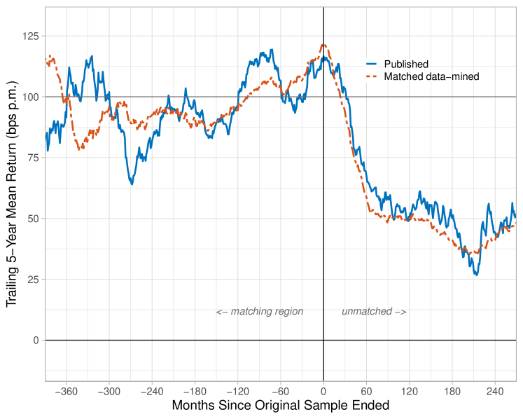
Out-of-sample, peer-reviewed and data-mined predictors perform similarly. For both groups, the trailing 5-year return increases to about 120 bps per month just as the sample ends, and then drops to around 60 bps per month five years after the sample ends. For both groups, returns hover around 40-60 bps per month for the remainder of the event time horizon.
These results imply that data mining works just as well as reading peer-reviewed journals. Back-testing accounting signals, unguided by theory, leads to the same out-of-sample returns as drawing on the best ideas from the best finance departments in the world. We emphasize that these accounting signals are very simple functions and are selected with the simplest of statistical methods. A typical finance undergraduate should be able to understand these methods, though it may take a bit of computer science training to code up the algorithm.
Of course, academic publications can destroy return predictability by publicizing mispricing ([41]). So the similar performance in Figure 2 may be due to offsetting effects. It could be that peer-reviewed predictability would have out-performed, if not for the publicization of mispricing.
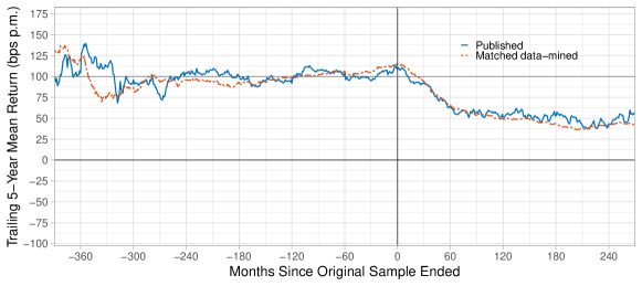
Figure 3a zooms in these results by separating out predictors by peer-reviewed theories. Panel (a) shows predictors that peer review attributes to risk. These predictors should not have offsetting effects related to the elimination of mispricing—if the peer-reviewed theories are correct. However, Panel (a) shows predictors founded in equilibrium theory perform no better than data mining. Risk-based predictability appears stronger in the first few years out-of-sample, but this outperformance vanishes around year 7. Since the publication dates are typically 4 years after the original samples end, it is not until around year 7 that the trailing 5-year mean return is fully out-of-sample.
The plot shows long-short returns in event time, where the event is the end of the original sample periods. Predictors are normalized to have 100 bps mean return in-sample. Data-mined predictors come from building ratios or scaled first differences of 240 accounting variables as described in Section 4.1. Matching is described in Table 4.3. For all categories of theory, theory and data mining lead to similar post-sample returns.
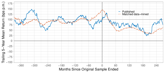
Panels (b) and (c) of Figure 3a examine mispricing and agnostic predictors, respectively. For both types of predictors, out-of-sample predictability is similar to that obtained from naive data mining. For the mispricing-based predictors, the published (solid) and data-mined (dot-dash) lines are so similar it looks as if they are all operating on the same underlying mechanism. The agnostic predictors outperform, but the difference is comparable to the standard error of roughly 20 bps per month seen in Table 3.
Overall, the similarity between data-mined and published returns suggests a different view of the [41] facts. McLean and Pontiff argue that investors learn about mispricing from academic publications, as seen in the fact that predictability systematically decays after publication. But investors are surely learning from the accounting data itself. One wonders, then, how much academics contribute. Figure 2 suggests that the contribution is minor. It looks as if both academics and investors are learning from the accounting data in parallel. Once evidence of predictability becomes strong enough, both investors and academics act, the former to correct the mispricing, and the latter to document it scientifically.
4.5 A Closer Look at Value and Momentum
How, exactly, does data mining achieve reseach-like out-of-sample returns? Tables 4.5 and 4.5 take a closer look, by listing the data-mined predictors that matched with Fama and French’s \citeyearparfama1992cross B/M and Jegadeesh and Titman’s \citeyearparjegadeesh1993returns 12-month momentum.
Table lists 20 of the 171 data-mined signals that performed similarly to Fama and French’s \citeyearparfama1992cross B/M in the original 1963-1990 sample period in terms of mean returns and t-stats. Signals are ranked according to the absolute difference in mean in-sample return. Sign = -1 indicates that a high signal implies a lower mean return in-sample. Data mining picks up themes found by peer-reviewed research (e.g. investment, equity issuance, accruals) and leads to similar out-of-sample performance as Fama and French’s B/M.
Table 4.5 begins with B/M. At the top of the table, we see that predictors related to asset growth had in-sample performance extremely similar to B/M, as did predictors related to depreciation and equity issuance. Moving down the table, we see predictors that are somewhat more distant, but that still achieved mean returns within 20 bps of B/M. These predictors include those related to cost growth and working capital investment. Still other predictors that performed similarly to B/M in-sample include one related to debt issuance.
Table lists 20 of the 44 data-mined signals that performed similarly to Jegadeesh and Titman’s \citeyearparjegadeesh1993returns 12-month momentum in the original 1964-1989 sample period in terms of mean returns and t-stats. Signals are ranked according to the absolute difference in mean in-sample return. Sign = -1 indicates that a high signal implies a lower mean return in-sample. Data mining picks up themes found by peer-reviewed research (e.g. profitabitability, investment) and leads to similar out-of-sample performance as Jegedeesh and Titman’s momentum.
Table 4.5 lists data-mined predictors that performed similarly to Jegadeesh and Titman’s (1993) 12-month momentum. Many themes seen in Table 4.5 show up again in Table 4.5, though we also see profitability-related predictors, as well as some unusual variables (rental expense). The Appendix lists predictors related to Banz’s (1981) Size predictor (Table A.4), which also include well-known themes (investment and profitability) and more unusual variables (investment tax credits and interest expense).
Overall, the themes seen in Tables 4.5 and 4.5 echo those found in the cross-sectional predictability literature. One may have thought that linking investment or profitability to expected returns requires Ph.D.-level insight. But it turns out that data mining based on basic accounting principles can systematically uncover these patterns. And while one may have thought that economic insight is required to find the out-of-sample robustness found in Fama and French’s \citeyearparfama1992cross B/M, it turns out this is not the case. On average, the data-mined predictors in Table 4.5 returned 69 bps in the 30 years after Fama and French’s sample, slightly higher than the 62 bps of B/M. Similarly, the data-mined counterparts to momentum earned 48 bps per month out-of-sample, not far from the 66 bps earned by momentum. Data-mined counterparts to Banz’s (1981) Size also performed similarly (Table A.4).
5 Alternative Data Mining and Theory Measures
This section uses robustness tests to help pin down the mechanism. Section 5.1 shows the key to replicating our main result is to data mine accounting variables instead of say, ticker symbols, and to screen variables for something resembling statistical significance.
Section 5.2 shows our results are not due to correlations with the published predictors. Section 5.3 show factor model measures of risk lead to similar results. Section 5.4 shows decay also happens for predictors based on highly rigorous theories.
5.1 Even More Naive Data Mining Procedures
How easy is it to data mine for Journal of Finance-like out-of-sample returns? To answer this question, we examine mining procedures that are even more naive than our baseline method.
We examine the following data mining methods:
-
1.
Screen 29,000 accounting-based strategies for in the published sample periods, where is, say, 2.0.
-
2.
Screen 29,000 accounting-based strategies for in the top of in the published sample periods, where is, say, 5%.
-
3.
Screen 3,160 ticker-based long short strategies using methods 1 and 2 above. The ticker-based strategies are constructed following [29].
[29] does not provide the algorithm but states that he asked his research assistant to “form portfolios based on the first, second, and third letters of the ticker symbol” and that the algorithm leads to 3,160 long-short portfolios. We interpret his instructions as follows: Generate 26 portfolios by going long all stocks with a first ticker letter of “A,” “B,” “C,” …, “Z.” Generate 26 portfolios by doing the same for the second ticker letter, and add a 27th portfolio for tickers that no second ticker letter. Apply the same to the third ticker. Repeating for the first three ticker letters results in long portfolios. Finally, form 80 choose 2 = 3,160 long-short portfolios by selecting all distinct pairs of the 80 long portfolios.
Figure 4b shows the resulting event-time returns. Screening accounting strategies for (Panel (a)) or for in the top 5% of in-sample t-stats (Panel (b)) leads to post-sample returns that are just a touch lower than those obtained from top journals. Thus, there is nothing special about the t-statistics and mean returns published in the journals. Just screening for statistical significance does the trick.
Instead of screening data mined strategies to match published in-sample statistics (Figure 2), we screen to have a minimum t-stat (Panels (a) and (c)) or to be in the top X% of data-mined t-stats (Panels (b) and (d)). Mining tickers (dotted) constructs 3,160 portfolios based on ticker symbols, following [29]. Extremely naive data mining generates research-like out-of-sample returns, though mining tickers is too naive.
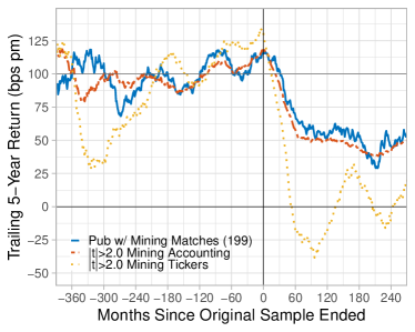
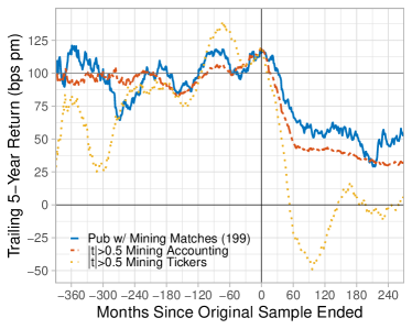
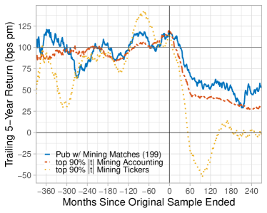
One cannot be so naive as to think that tickers contain information about expected returns, however. The dotted lines in Panels (a) and (b) show that data-mined ticker strategies with or in the top 5% of yield zero out-of-sample returns, on average. These results illustrate how sample mean returns do not necessarily measure expected returns and how data mining bias depends on the dataset being mined (Equation (4)).
One cannot also be so naive as to ignore statistical significance. Panel (c) shows that data-mined accounting strategies with leads to out-of-sample returns that are roughly 20% lower than found from journals. Similar underperformance is found among the top 90% of data-mined accounting strategies (dropping only the worst 10% of ), shown in Panel (d). These results show that published research contains more information about out-of-sample returns than just the sign of in-sample returns. But the other results in Figure 4b shot research does not contain much more information than the sign.
Overall, these alternative data mining exercises show that it is surprisingly easy to find out-of-sample returns comparable to those found in the Journal of Finance and similar outlets.
5.2 Data Mining Excluding Correlated Returns
In risk-based theories, expected returns are driven by correlations with risk factors. Since our data-mined predictors are selected to have in-sample mean returns that match published predictors, one might conjecture that correlations drive our results.
Figure 5b rules out this explanation. As in Section 4.3, we match each published strategy with data-mined strategies by keeping data-mined strategies with similar in-sample mean returns and t-stats. But now we add the requirement that a matched strategy should have returns that are less than 10% correlated with the published strategy returns. The key features of Figures 2 and 3a continue to hold: Data-mined and published predictors perform similarly post-sample, it does not matter if the published predictors are based on a risk or mispricing, and data-mining captures the rise and fall in returns around the end of the original sample periods.
We match data-mined with published strategies based on in-sample mean returns and t-stats (as in Figures 2-3a) but now we drop data-mined strategies if they have returns that are more than 10% correlated with published strategies (in-sample). This drops five actual signals for which there are no matched strategies with correlation less than 10% (AssetGrowth, BM, dNoa, Frontier, NOA). The similarity in out-of-sample returns is not driven by correlations.
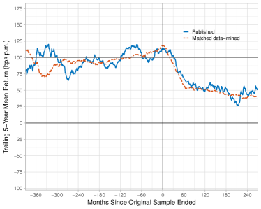
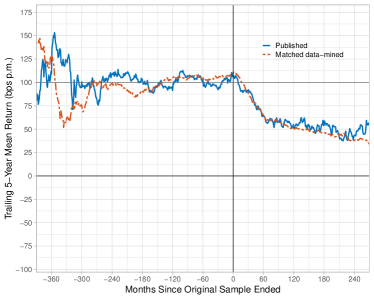
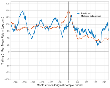
This robustness is natural given the summary statistics from our baseline matching process (Table 4.2). The matched data-mined predictors have a median correlation of 7% with the published predictor. These correlations are reminiscent of the low correlations found among published predictor returns ([41]; [13]).
5.3 Factor Model Measures of Risk
Factor models are commonly used to measure risk in the asset pricing literature. This section examines whether risk as measured by the CAPM, Fama-French 3 (FF3), and Fama-French 5 (FF5) factor models help predict out-of-sample returns.
For each published long-short portfolio , we estimate exposure to factor using time-series regressions on the original papers’ sample periods. According to the factor models, the estimated expected return is , where is the in-sample mean return of factor . [23] state that with respect to their SMB and HML factors have “a clear interpretation as risk-factor sensitivities.” If this interpretation is both correct and stable, then the estimated expected return should remain out-of-sample.555[25] are more cautious, and describe the risk-based ICAPM as “the more ambitious interpretation” of the five factor model.
Figure 6b plots the post-sample mean return against the factor model expected returns. We normalize by the in-sample mean return for ease of interpretation. With this normalization, the position on the x-axis ([Predicted by Risk Model]/[In-Sample]) represents the share of predictability due to risk.
Each marker is one published long-short strategy. [Post-Sample]/[In-Sample] is the mean return post-sample divided by the mean return in-sample. [Predicted by Risk Model] is , where is the in-sample mean return of factor and comes from an in-sample time series regression of long-short returns on factor realizations. FF3 and FF5 are the Fama-French 3- and 5-factor models. The blue line is the OLS fit. The axes zoom in on the interpretable region of the chart and omits outliers. Factor models attribute a minority of in-sample predictability to risk, at best. Post-sample decay is the distance between the horizontal line at 1.0 and the regression line, and this decay is near 50% even for predictors that are entirely due to risk according to the CAPM and FF3. For FF5, decay is smaller for predictors that are more than 75% due to risk, but these predictors are rare.
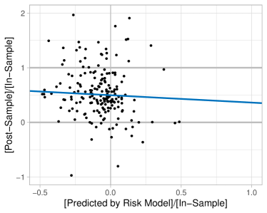
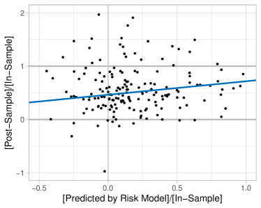
The figure shows that a minority of in-sample predictability is attributed to risk, at best. Using the CAPM (Panel (a)), nearly all predictability is less than 25% due to risk (to the left of the vertical line at 0.25), and many predictors have a negative risk share. FF3 (Panel (b)) implies more predictability is due to risk, but still the vast majority of predictors lie to the left of 0.50. FF5, which in the more ambitious interpretation is due to risk ([25]), implies that a non-trivial minority of predictors are more than 50% due to risk, but only a handful of predictors are more than 75% due to risk. These results are consistent with our manual reading of the papers, which typically attribute predictability to mispricing (Table 2).
The regression line in Figure 6b smooths out the noise in post-sample returns and provides a simple interpretation: the distance between the horizontal line at 1.0 and the regression line measures the out-of-sample decay for a given level of risk. In all panels, this distance is close to 0.5 for the majority of relevant risk shares. The risk model that has strongest relationship with post-sample returns is FF5, and even the rare predictors which are 75% due to risk according to FF5 decay by roughly 40% out-of-sample.
5.4 More Rigorous Theories
Our primary theory categories do not differentiate between more- and less-rigorous risk theories. Figure 7 takes a closer look at the risk theories by plotting the out-of-return against the count of risk to mispricing words.
Each marker represents one published predictor’s mean return. The regression line is fitted with OLS. The full reference for each acronym can be found at https://github.com/OpenSourceAP/CrossSection/blob/master/SignalDoc.csv. Even predictors with the strongest focus on risk decay on average.
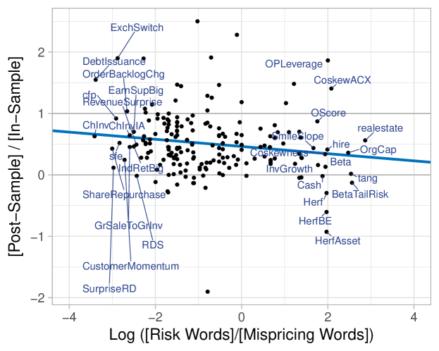
Predictors on the right of the figure are often full blown quantitative equilibrium models. For example, “realestate” is based on [50]’s general equilibrium production economy with heterogeneous firms. She computes equilibrium using numerical methods rather than artificially simplifying model for tractability. She also calibrates the model to match important moments in the data to show her model is not just a qualitative description of the economy, but that it is a quantiative match. Nevertheless, Figure 7 shows that her predictor decays by roughly 50% out-of-sample, and in this sense is no different than a typical predictor based on verbal mispricing arguments.
Other predictors on the right of Figure 7 include “OrgCap” from [21], “hire” from [6], “Cash” from [45], and “InvGrowth” from [5]. All of these papers include quantitative equilibrium models and yet all of these predictors decay notably post-sample, in-line with predictors based on mispricing arguments.
6 Conclusion
We provide an empirical test of whether asset pricing theory helps predict the cross-section of stock returns. Our test examines whether out-of-sample performance depends on the theoretical explanation generated by the peer-review process. We find that the answer is no: the theoretical origins matter little, and indeed out-of-sample returns are roughly the same if the predictor is simply mined from Compustat.
Based on our meta-theory, the empirical results imply that consistency with risk-based theory does not provide a signal of higher and more stable expected returns. This result is consistent with survey studies, which consistently find that academic theories of risk are largely overlooked in practice ([43]; [14]; [7]). In fact, academic risk factors are even overlooked by finance academics in their real-life investing ([19]).
Though our findings are negative for asset pricing theory, they are quite positive for the growing literature on machine learning in finance. Consistent with [52], we find that naive data mining generates substantial “out-of-sample” returns, providing a kind of fundamental justification for more sophiscated machine learning methods. Indeed, data mined returns are just as large as those found through the academic research. This result suggests that a way forward in asset pricing is to, at least for now, let the data speak directly, without the filters from traditional theory, following the lead of fields like protein folding and linguistics.
Appendix A Appendix
A.1 More General Model and Proof of Proposition 1
This general model nests the one in the main text. For clarity, we restate all assumptions here (this section is self-contained).
A.1.1 A More General Model of Data Mining and Decay
The return on strategy in month is given by
| (9) |
allows for expected returns shifting closer to zero out-of-sample
| (10) |
where
Define
and similarly for and . We assume out-of-sample residuals are unpredictable with in-sample information:
where represents anything known in-sample (e.g. ).
Let represent a set of data-mined strategies, a set of strategies consistent with theory, and . These sets are chosen using only in-sample data, so and
| (11) |
A.1.2 Cochrane’s Hope, the General Case
The general case requires a more nuanced definition of a helpful theory
Definition 2.
[General case] is helpful compared to if
| (12) | ||||
| (13) |
This definition just says that a helpful theory finds higher and more stable expected returns compared to data mining, once you account for the signs. This definition does not require and thus nests the definition in the main text.
The general case has a more nuanced definition of out-of-sample decay:
| (14) |
where allows for switching signs in case .
We now state a more general form of Cochrane’s Hope:
Once again, this more general proposition nests the main text’s if we enforce .
Proof.
The expected decay can be written as
Use the law of iterated expectations and Equation (11) to remove
| (15) |
Now we work on the expectation conditioning on a specific :
where the second line plugs in and third line uses Equation (10).
Then plug in and apply the definition of a helpful theory:
Integrate over and plugging into Equation (15) finishes the proof. ∎
A.2 Risk words and mispricing words
We remove stopwords, lowercase and lemmatize all words using standard methods. Then, we count separately the words corresponding to risk and mispricing.
We consider as risk words the following terms and their grammatical variations: "utility," "maximize," "minimize," "optimize," "premium," "premia," "premiums," "consume," "marginal," "equilibrium," "sdf," "investment-based," and "theoretical." We also count as risk words appearances of “risk” that are not preceded by “lower,” and appearances of “aversion,” “rational,” and “risky” that are not preceded by “not.”
The mispricing words consist of " "anomaly," "behavioral," "optimistic," "pessimistic," "sentiment," "underreact," "overreact," "failure," "bias," "overvalue," "misvalue," "undervalue," "attention," "underperformance," "extrapolate," "underestimate," "misreaction," "inefficiency," "delay," "suboptimal," "mislead," "overoptimism," "arbitrage," "factor unlikely," and their grammatical variations. We further count as mispricing the terms "not rewarded," "little risk," "risk cannot [explain]," " low [type of] risk," "unrelated [to the type of] risk," "fail [to] reflect," and "market failure," where the terms in brackets are captured using regular expressions or correspond to stopwords.
A.3 Follow-Up Citations Method
To analyze the impact of the original papers, we examine each citation in follow-up research. Our process involves the following steps:
-
1.
Extraction of Contextual Data: For each citation in a follow-up paper, we extract a 500-character window around the citation of the original paper, providing context for analysis.
-
2.
Classification of Citations Using ChatGPT: We utilize ChatGPT, instructed as a finance academic expert, for categorizing each citation. The categories are based on the nature of the citation:
-
•
Methodological: The original paper’s methodology is referenced.
-
•
Incidental: The original paper is mentioned tangentially or for context.
-
•
Substantial: The original paper is critiqued or discussed in-depth.
-
•
Other: Citations that do not fit into the above categories.
-
•
-
3.
Categorization Outcome: Citations are classified as methodological, incidental, substantial, or other, based on ChatGPT’s analysis.
The corresponding prompt is:
You are a finance academic expert analyzing citations. Your task: categorize how ’citation’ is referenced in a given text.
Methodological: Refers to citation’s methodology.
Incidental: Mentions citation tangentially or just for context.
Substantial: Criticizes or discusses citation in-depth.
Other: Doesn’t fit the above categories.
Please respond as CATEGORY:X
A.4 Additional Empirical Results
As in Table 4.2, each June, we sort strategies into 5 bins based on their past 30-year mean returns (“in-sample”), and then compute the mean return over the next year within each bin (“out-of-sample”). But now we only examine bins sorted 2003-2019. Data-mining predictability is weaker post-2003, especially in large stocks.
We list peer-reviewed predictors that have zero matched data-mined accounting signals. All of the failed matches have extremely large in-sample t-stats. Most of the failed matches use non-accounting data (e.g. option prices, analyst forecasts), suggesting expanding the data-mined dataset would mostly complete the matching process, though the benefit may not be worth the cost.
Inst own among high short interest Mispricing 240.9 3.35 Chan, Jegadeesh and Lakonishok (1996) Earnings announcement return Mispricing 119.4 12.98 Chan, Jegadeesh and Lakonishok (1996) Earnings forecast revisions Mispricing 113.9 8.87 Hartzmark and Salomon (2013) Dividend seasonality Mispricing 32.8 14.38 Hou (2007) Industry return of big firms Mispricing 229.5 9.39 Loh and Warachka (2012) Earnings surprise streak Mispricing 108.9 10.42 Richardson et al. (2005) Change in financial liabilities Mispricing 72.6 12.08 Spiess and Affleck-Graves (1999) Debt issuance Mispricing 21.3 3.94 Zhang (2006) Firm age - momentum Mispricing 232.9 5.37
Jegadeesh (1990) Short term reversal Agnostic 292.5 14.20 Novy-Marx (2012) Intermediate momentum Agnostic 123.7 5.86
Table lists 20 of the 221 data-mined signals that performed similarly to Banz’s \citeyearparbanz1981relationship size in the original sample period. Signals are ranked according to the absolute difference in mean in-sample return. Sign = -1 indicates that a high signal implies a lower mean return in-sample. Data mining leads to similar out-of-sample performance.
This table lists the number of signals by theory and published journal. Finance journals find risk explanations more frequently than accounting journals, but risk explanations still account for a small minority of predictors in finance journals.
| Agnostic | Mispricing | Risk | |
|---|---|---|---|
| AR | 1 | 14 | 0 |
| BAR | 0 | 1 | 0 |
| Book | 2 | 0 | 0 |
| CAR | 0 | 1 | 0 |
| FAJ | 1 | 1 | 0 |
| JAE | 3 | 14 | 0 |
| JAR | 3 | 2 | 0 |
| JBFA | 0 | 1 | 0 |
| JEmpFin | 0 | 1 | 0 |
| JF | 16 | 35 | 12 |
| JFE | 16 | 22 | 6 |
| JFM | 0 | 2 | 0 |
| JFQA | 0 | 3 | 2 |
| JFR | 0 | 0 | 1 |
| JOIM | 0 | 1 | 0 |
| JPE | 0 | 0 | 3 |
| JPM | 1 | 0 | 0 |
| MS | 0 | 2 | 2 |
| Other | 0 | 1 | 0 |
| RAS | 0 | 5 | 1 |
| RED | 0 | 0 | 1 |
| RFQA | 0 | 1 | 0 |
| RFS | 0 | 7 | 7 |
| ROF | 0 | 1 | 3 |
| WP | 1 | 1 | 0 |
References
- [1] Jeffery S Abarbanell and Brian J Bushee “Abnormal returns to a fundamental analysis strategy” In Accounting Review JSTOR, 1998, pp. 19–45
- [2] Turan G Bali, Robert F Engle and Scott Murray “Empirical asset pricing: The cross section of stock returns” John Wiley & Sons, 2016
- [3] Rolf W Banz “The relationship between return and market value of common stocks” In Journal of financial economics 9.1 Elsevier, 1981, pp. 3–18
- [4] Christopher B Barry and Stephen J Brown “Differential information and the small firm effect” In Journal of financial economics 13.2 Elsevier, 1984, pp. 283–294
- [5] Frederico Belo and Xiaoji Lin “The inventory growth spread” In The Review of Financial Studies 25.1 Society for Financial Studies, 2012, pp. 278–313
- [6] Frederico Belo, Xiaoji Lin and Santiago Bazdresch “Labor hiring, investment, and stock return predictability in the cross section” In Journal of Political Economy 122.1 University of Chicago Press Chicago, IL, 2014, pp. 129–177
- [7] Svetlana Bender, James J Choi, Danielle Dyson and Adriana Z Robertson “Millionaires speak: What drives their personal investment decisions?” In Journal of Financial Economics 146.1 Elsevier, 2022, pp. 305–330
- [8] Paul Calluzzo, Fabio Moneta and Selim Topaloglu “When anomalies are publicized broadly, do institutions trade accordingly?” In Management Science 65.10 INFORMS, 2019, pp. 4555–4574
- [9] Andrew Y Chen “Most claimed statistical findings in cross-sectional return predictability are likely true” In arXiv preprint arXiv:2206.15365, 2022
- [10] Andrew Y Chen and Mihail Velikov “Zeroing in on the Expected Returns of Anomalies” In Journal of Financial and Quantitative Analysis, 2022
- [11] Andrew Y Chen and Tom Zimmermann “Publication bias and the cross-section of stock returns” In The Review of Asset Pricing Studies 10.2 Oxford University Press, 2020, pp. 249–289
- [12] Andrew Y Chen and Tom Zimmermann “Publication Bias in Asset Pricing Research” In arXiv preprint arXiv:2209.13623, 2022
- [13] Andrew Y. Chen and Tom Zimmermann “Open Source Cross Sectional Asset Pricing” In Critical Finance Review, 2022
- [14] Alex Chinco, Samuel M Hartzmark and Abigail B Sussman “A new test of risk factor relevance” In The Journal of Finance 77.4 Wiley Online Library, 2022, pp. 2183–2238
- [15] Alex Chinco, Andreas Neuhierl and Michael Weber “Estimating the anomaly base rate” In Journal of financial economics 140.1 Elsevier, 2021, pp. 101–126
- [16] Tarun Chordia, Avanidhar Subrahmanyam and Qing Tong “Have capital market anomalies attenuated in the recent era of high liquidity and trading activity?” In Journal of Accounting and Economics 58.1 Elsevier, 2014, pp. 41–58
- [17] Charles Clarke “The level, slope, and curve factor model for stocks” In Journal of Financial Economics 143.1 Elsevier, 2022, pp. 159–187
- [18] John H Cochrane “Asset pricing: Revised edition” Princeton university press, 2009
- [19] James Doran and Colbrin Wright “What Really Matters When Buying and Selling Stocks?” In Financial Education 8.1, 2007, pp. 35–61
- [20] Bradley Efron “Large-scale inference: empirical Bayes methods for estimation, testing, and prediction” Cambridge University Press, 2012
- [21] Andrea L Eisfeldt and Dimitris Papanikolaou “Organization capital and the cross-section of expected returns” In The Journal of Finance 68.4 Wiley Online Library, 2013, pp. 1365–1406
- [22] Eugene F Fama and Kenneth R French “The cross-section of expected stock returns” In the Journal of Finance 47.2 Wiley Online Library, 1992, pp. 427–465
- [23] Eugene F Fama and Kenneth R French “Common risk factors in the returns on stocks and bonds” In Journal of financial economics 33.1 Elsevier, 1993, pp. 3–56
- [24] Eugene F Fama and Kenneth R French “Luck versus skill in the cross-section of mutual fund returns” In The journal of finance 65.5 Wiley Online Library, 2010, pp. 1915–1947
- [25] Eugene F Fama and Kenneth R French “A five-factor asset pricing model” In Journal of financial economics 116.1 Elsevier, 2015, pp. 1–22
- [26] Andrea Frazzini and Lasse Heje Pedersen “Betting against beta” In Journal of Financial Economics 111.1 Elsevier, 2014, pp. 1–25
- [27] Shingo Goto and Toru Yamada “False Alpha and Missed Alpha: An Out-of-Sample Mining Expedition” In Working Paper, 2022
- [28] Samuel M Hartzmark and David H Solomon “The dividend month premium” In Journal of Financial Economics 109.3 Elsevier, 2013, pp. 640–660
- [29] Campbell R Harvey “Presidential address: The scientific outlook in financial economics” In The Journal of Finance 72.4 Wiley Online Library, 2017, pp. 1399–1440
- [30] Campbell R Harvey and Yan Liu “False (and missed) discoveries in financial economics” In The Journal of Finance 75.5 Wiley Online Library, 2020, pp. 2503–2553
- [31] Campbell R Harvey, Yan Liu and Heqing Zhu “… and the cross-section of expected returns” In The Review of Financial Studies 29.1 Oxford University Press, 2016, pp. 5–68
- [32] Robert A Haugen and Nardin L Baker “Commonality in the determinants of expected stock returns” In Journal of financial economics 41.3 Elsevier, 1996, pp. 401–439
- [33] Narasimhan Jegadeesh and Sheridan Titman “Returns to buying winners and selling losers: Implications for stock market efficiency” In The Journal of finance 48.1 Wiley Online Library, 1993, pp. 65–91
- [34] Michael C. Jensen and George A. Benington “Random Walks and Technical Theories: Some Additional Evidence” In The Journal of Finance 25.2, 1970, pp. 469–482
- [35] Theis Ingerslev Jensen, Bryan Kelly and Lasse Heje Pedersen “Is there a replication crisis in finance?” In The Journal of Finance Wiley Online Library, 2022
- [36] John Jumper et al. “Highly accurate protein structure prediction with AlphaFold” In Nature 596.7873 Nature Publishing Group, 2021, pp. 583–589
- [37] Serhiy Kozak, Stefan Nagel and Shrihari Santosh “Interpreting factor models” In The Journal of Finance 73.3 Wiley Online Library, 2018, pp. 1183–1223
- [38] Jonathan Lewellen, Stefan Nagel and Jay Shanken “A skeptical appraisal of asset pricing tests” In Journal of Financial economics 96.2 Elsevier, 2010, pp. 175–194
- [39] Andrew W Lo and A Craig MacKinlay “Data-snooping biases in tests of financial asset pricing models” In The Review of Financial Studies 3.3 Oxford University Press, 1990, pp. 431–467
- [40] Andreu Mas-Colell, Michael Dennis Whinston and Jerry R Green “Microeconomic theory” Oxford university press New York, 1995
- [41] R David McLean and Jeffrey Pontiff “Does academic research destroy stock return predictability?” In The Journal of Finance 71.1 Wiley Online Library, 2016, pp. 5–32
- [42] R David McLean, Jeffrey Pontiff and Christopher Reilly “Taking sides on return predictability” In Georgetown McDonough School of Business Research Paper, 2020
- [43] Liliya Mukhlynina and Kjell G Nyborg “The Choice of Valuation Techniques in Practice: Education Versus Profession” In Critical Finance Review 9.1-2 Now Publishers Inc., 2020, pp. 201–265
- [44] Robert Novy-Marx and Mihail Velikov “A taxonomy of anomalies and their trading costs” In The Review of Financial Studies 29.1 Oxford University Press, 2016, pp. 104–147
- [45] Berardino Palazzo “Cash holdings, risk, and expected returns” In Journal of Financial Economics 104.1 Elsevier, 2012, pp. 162–185
- [46] Mark T Soliman “The use of DuPont analysis by market participants” In The Accounting Review 83.3, 2008, pp. 823–853
- [47] Hugo Sonnenschein “Market excess demand functions” In Econometrica: Journal of the Econometric Society JSTOR, 1972, pp. 549–563
- [48] Ryan Sullivan, Allan Timmermann and Halbert White “Data-snooping, technical trading rule performance, and the bootstrap” In The journal of Finance 54.5 Wiley Online Library, 1999, pp. 1647–1691
- [49] Ryan Sullivan, Allan Timmermann and Halbert White “Dangers of data mining: The case of calendar effects in stock returns” In Journal of Econometrics 105.1 Elsevier, 2001, pp. 249–286
- [50] Selale Tuzel “Corporate real estate holdings and the cross-section of stock returns” In The Review of Financial Studies 23.6 Oxford University Press, 2010, pp. 2268–2302
- [51] Shu Yan “Jump risk, stock returns, and slope of implied volatility smile” In Journal of Financial Economics 99.1 Elsevier, 2011, pp. 216–233
- [52] Xuemin Sterling Yan and Lingling Zheng “Fundamental analysis and the cross-section of stock returns: A data-mining approach” In The Review of Financial Studies 30.4 Oxford University Press, 2017, pp. 1382–1423
- [53] Paolo Zaffaroni and Guofu Zhou “Asset Pricing: Cross-section Predictability” In Available at SSRN 4111428, 2022
- [54] Wayne Xin Zhao et al. “A Survey of Large Language Models”, 2023 arXiv:2303.18223 [cs.CL]