Steel Phase Kinetics Modeling using
Symbolic Regression

Abstract

We describe an approach for empirical modeling of steel phase kinetics based on symbolic regression and genetic programming. The algorithm takes processed data gathered from dilatometer measurements and produces a system of differential equations that models the phase kinetics. Our initial results demonstrate that the proposed approach allows to identify compact differential equations that fit the data. The model predicts ferrite, pearlite and bainite formation for a single steel type. Martensite is not yet included in the model. Future work shall incorporate martensite and generalize to multiple steel types with different chemical compositions.

I Introduction

Steels are alloys consisting of the main elements iron and carbon and often contain additional elements, which may be deliberate additions for beneficial effects or be present as limited but unavoidable residuals from steelmaking, so called tramp elements. All of these elements are incorporated in the crystalline solid microstructure, which directly affects the properties and performance of the steel [1]. The fact that pure iron has two different crystalline structures at different temperatures allow for steelmaking with great versatility [2]: Austenite at high temperatures ($912\text{\,}\mathrm{\SIUnitSymbolCelsius}$ – $1394\text{\,}\mathrm{\SIUnitSymbolCelsius}$) and ferrite at low and room temperatures ($912\text{\,}\mathrm{\SIUnitSymbolCelsius}$).

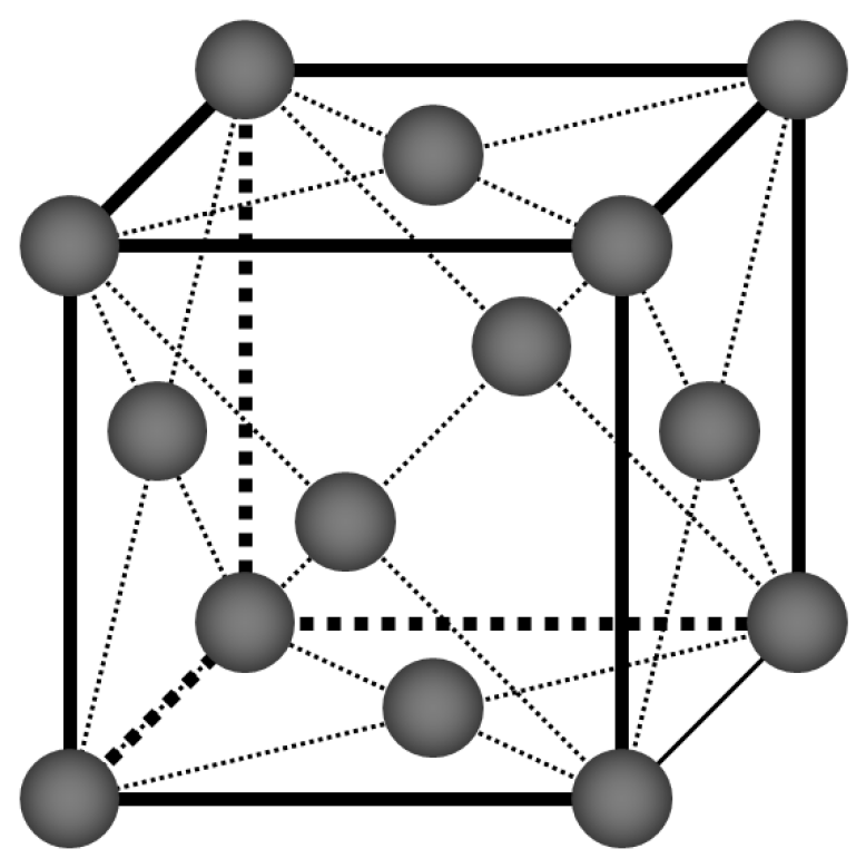
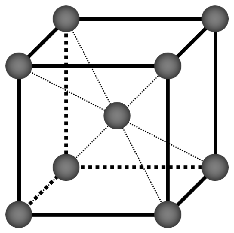
The crystal structures of pure iron are shown in Figure 1. The shown unit cells define the repeating iron atom arrangements in the crystal. For austenite the structure is face-centered cubic (FCC), for ferrite body-centered cubic (BCC). The FCC structure of austenite is more densely packed than the BCC structure of ferrite, leading to a volume change of approximately 1–3% for the austenite to ferrite transformation [3]. Dilatometry is a technique that utilizes the change in volume to study phase transformations [4].

A Face-centered cubic structure: Atoms are on each corner and the centers of each face of the cube.

B Body-centered cubic structure: Atoms are on each corner and the center of the cube.

Figure 1: FCC and BCC structures.

Heat treatment can be used to achieve desired mechanical steel properties such as hardness, strength, ductility or toughness, which are dependent on microstructure and grain size [5]. Steel which is heated to its austenitising temperature may transform to different phases during cooling, each providing a unique combination of properties. Some of these transformations products are (listed in order of their formation with increasing cooling velocity):

• Ferrite: BCC crystal structure with other elements in solid solution.

• Pearlite: Phase consisting of alternate lamellae of ferrite and cementite (iron carbide, $Fe_{3}C$), formed on slow cooling.

• Bainite: Non-lamellar mixture of ferrite and carbides, which can be classified into upper and lower bainite. Upper bainite consists of plates of cementite in a matrix of ferrite. Lower bainite consists of ferrite needles containing carbide platelets

• Martensite: Metastable phase resulting from the diffusionless athermal decomposition of austenite below a certain temperature at sufficiently high cooling rates.

I-A Transformation model

To model the transformation behavior of austenite to its transformation products many models exist, which often rely on the Johnson-Mehl-Avrami-Kolmogorov model (JMAK) [6, 7, 8, 9, 10].

The basic equation for isotherm transformation reads as $X=1-\exp(-kt^{n})$, where $X$ is the volume of the transformed phase, and $k$ and $n$ are material dependent parameters.

JMAK models may incorporate different nucleation and growth theories and are applicable for the transformation of austenite to ferrite, pearlite and bainite. To describe the transformation to martensite, most commonly the Koistinen-Marburger equation or a variation of it is used [11]: $X=1-\exp(-\alpha(M_{s}-T))$, where $\alpha$ is a parameter, $\alpha\approx 0.011$, $M_{s}$ is the martensite start temperature (highest temperature at which martensite can form) and $T$ the temperature of the sample, which is cooled below $M_{s}$.

Further information on steels with complex microstructures and various modeling approaches can be found in [12].

II Data Acquisition

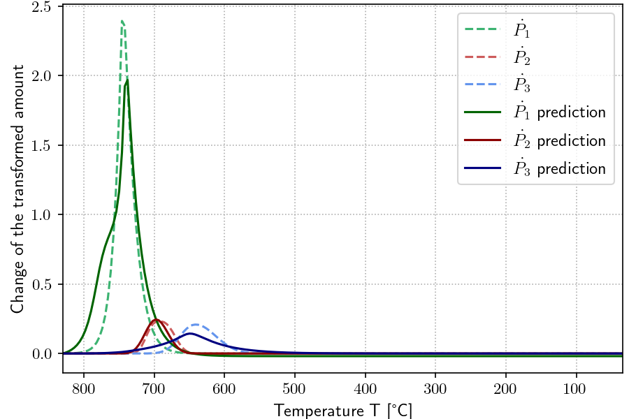
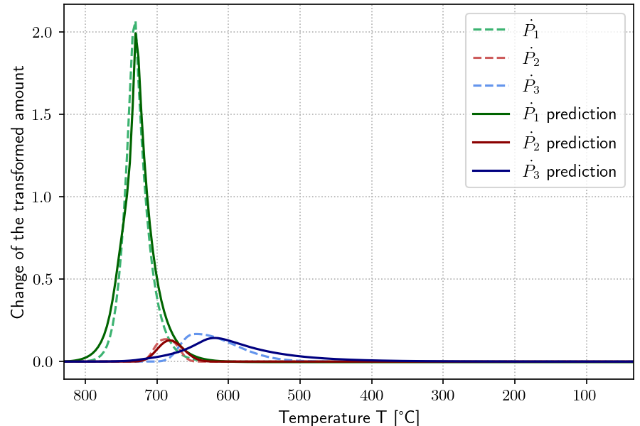
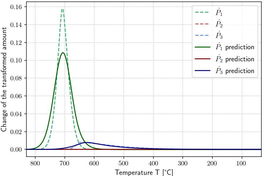
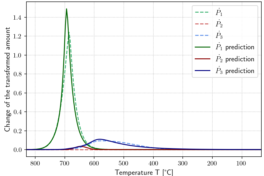
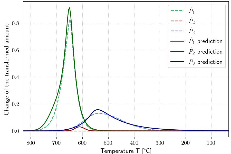
The data is obtained by dilatometer measurements of one steel type. Several measurements with different cooling rates ranging from $0.6\text{\,}\unit\mathrm{[}\mathrm{p}\mathrm{e}\mathrm{r}\mathrm{-}\mathrm{m}\mathrm{o}\mathrm{d}\mathrm{e}\mathrm{=}\mathrm{f}\mathrm{r}\mathrm{a}\mathrm{c}\mathrm{t}\mathrm{i}\mathrm{o}\mathrm{n}\mathrm{]}{\mathrm{K}\mathrm{/}\mathrm{s}}$ to $120\text{\,}\unit\mathrm{[}\mathrm{p}\mathrm{e}\mathrm{r}\mathrm{-}\mathrm{m}\mathrm{o}\mathrm{d}\mathrm{e}\mathrm{=}\mathrm{f}\mathrm{r}\mathrm{a}\mathrm{c}\mathrm{t}\mathrm{i}\mathrm{o}\mathrm{n}\mathrm{]}{\mathrm{K}\mathrm{/}\mathrm{s}}$ were made. The data was processed and for the transformation rates, fits for each phase, based on additional information, were calculated such that the overall transformation is described by the transformation of the individual phases. The result of the data preprocessing are ten data files which contains the cooling rate ($Ks$), the temperature $T$, time $t$, the change rates of volume fractions ($\dot{P}_{1},\dot{P}_{2},\dot{P}_{3},\dot{P}_{4}$) and the retained fraction of austenite ($RA$). Because of the high computation time, we decided to use only five data files, which are shown in Figure 2. We used the combination of the data files to find a model that describes the kinetics for all cooling rates. In this first set of experiments we ignore martensite ($\dot{P}_{4}$).

III Modeling Approach

We used tree-based genetic programming (GP) with a multi-tree representation. Each solution candidate consists of four trees, whereby each tree represents one expression on the right hand side (RHS) of the system of differential equations (DE).

$$\ddot{P}_{1}= f_{P_{1}}(\dot{P}_{1},\dot{P}_{2},\dot{P}_{3},RA,Ks,T,\theta_{P_{1}})$$

$$\ddot{P}_{2}= f_{P_{2}}(\dot{P}_{1},\dot{P}_{2},\dot{P}_{3},RA,Ks,T,\theta_{P_{2}})$$

$$\ddot{P}_{3}= f_{P_{3}}(\dot{P}_{1},\dot{P}_{2},\dot{P}_{3},RA,Ks,T,\theta_{P_{3}})$$

$$\dot{RA}= f_{RA}(\dot{P}_{1},\dot{P}_{2},\dot{P}_{3},RA,Ks,T,\theta_{RA})$$

The expression trees are evolved using GP. The algorithm automatically selects features that are included in each expression. In the same way the functions and operators used in each expression are evolved automatically. We use the same function and terminal set for each expression and apply the same limits for the maximum number of nodes and the maximum depth of each tree.

The evolved expressions may also include numeric parameters $\theta$ which are memetically optimized as described in [13]. For fitness evaluation of a solution candidate we first solve the DE system using the measured initial values with a numeric integration scheme (RK45) and then compare to the target values for $\dot{P}_{1},\dot{P}_{2},\dot{P}_{3}$ and RA in the data files.

We used all data rows for training to check whether it is in principle possible to evolve a system of DE that fits the measured steel phase kinetics. An analysis of the expected error of the approach with separate training and test sets is left for future work.

III-A Algorithm Configuration

We used the Age-Layered Population Structure Genetic Algorithm (ALPS-GA), which was invented by Gregory S. Hornby [14]. Similar to the original Genetic Algorithm (GA) by J. Holland [15], is uses the same genetic cycle (with selection, crossover and mutation), but isolated for each age-layer. Each layer represents an age bracket with its own population. The only exception for this isolation is the selection operator, which typically selects parents out of a layer-overlapping mating pool. The default configuration for this mating pool is the current layer (wherein the selection operator is currently working) and the underlying layer with younger individuals. The first layer (youngest age bracket) is regularly reseeding with random individuals (defined by the age gap). New layers open up after a predefined aging scheme, which uses the age gap for calculation. The maximum number of layers is configurable. The age of an individual is defined as follows $1+\text{Age}_{\text{oldestParent}}$.

For this paper we tried several different parameter settings that produced good results with ALPS-GP for similar problems. A more detailed sensitivity analysis is left for future work. The parameter values are shown in table I. We use and extend the framework HeuristicLab[16] for this paper. More details about the assigned operators can be read in [17, 18].

[b] Parameter Value Crossover Subtree Swapping (Probability = 25%) Mutator Multi Symbolic Expression Tree Manipulator Mutation Probability 10% Elites 1 Population Size (per Layer) 200 Selector Generalized Rank (Pressure = 5) Mating Pool Range 1 (Current + Underlying) Age Gap 8 Aging Scheme Polynomial Age Layers 16 max. Generations 2000 Terminal Set State variables and real-valued parameters Function Set $+,\times,\div,x^{2},\exp,\tanh$, analytic quotient¹

• $AQ(x,y)=x/\sqrt{1+y^{2}}$

TABLE I: Parameter configuration for the ALPS-GA.

IV Results

Figure 2 shows data and predictions for five different cooling rates (in [per-mode=symbol]). Because we use all data rows for training, all predictions reflect the training set. Each panel in the figure shows the change rate of the transformed amount over temperature $T$, where $T$ ranges from $830\text{\,}\mathrm{\SIUnitSymbolCelsius}$ down to $34\text{\,}\mathrm{\SIUnitSymbolCelsius}$, for $\dot{P_{1}}$ (ferrite), $\dot{P_{2}}$ (pearlite) and $\dot{P_{3}}$ (bainite) as well as their predictions. At the current stage, the amount of $\dot{P}_{4}$ (martensite) is ignored.

A Cooling rate $0.6\text{\,}\unit\mathrm{[}\mathrm{p}\mathrm{e}\mathrm{r}\mathrm{-}\mathrm{m}\mathrm{o}\mathrm{d}\mathrm{e}\mathrm{=}\mathrm{f}\mathrm{r}\mathrm{a}\mathrm{c}\mathrm{t}\mathrm{i}\mathrm{o}\mathrm{n}\mathrm{]}{\mathrm{K}\mathrm{/}\mathrm{s}}$

B Cooling rate $2.5\text{\,}\unit\mathrm{[}\mathrm{p}\mathrm{e}\mathrm{r}\mathrm{-}\mathrm{m}\mathrm{o}\mathrm{d}\mathrm{e}\mathrm{=}\mathrm{f}\mathrm{r}\mathrm{a}\mathrm{c}\mathrm{t}\mathrm{i}\mathrm{o}\mathrm{n}\mathrm{]}{\mathrm{K}\mathrm{/}\mathrm{s}}$

C Cooling rate $10\text{\,}\unit\mathrm{[}\mathrm{p}\mathrm{e}\mathrm{r}\mathrm{-}\mathrm{m}\mathrm{o}\mathrm{d}\mathrm{e}\mathrm{=}\mathrm{f}\mathrm{r}\mathrm{a}\mathrm{c}\mathrm{t}\mathrm{i}\mathrm{o}\mathrm{n}\mathrm{]}{\mathrm{K}\mathrm{/}\mathrm{s}}$

D Cooling rate $40\text{\,}\unit\mathrm{[}\mathrm{p}\mathrm{e}\mathrm{r}\mathrm{-}\mathrm{m}\mathrm{o}\mathrm{d}\mathrm{e}\mathrm{=}\mathrm{f}\mathrm{r}\mathrm{a}\mathrm{c}\mathrm{t}\mathrm{i}\mathrm{o}\mathrm{n}\mathrm{]}{\mathrm{K}\mathrm{/}\mathrm{s}}$

E Cooling rate $80\text{\,}\unit\mathrm{[}\mathrm{p}\mathrm{e}\mathrm{r}\mathrm{-}\mathrm{m}\mathrm{o}\mathrm{d}\mathrm{e}\mathrm{=}\mathrm{f}\mathrm{r}\mathrm{a}\mathrm{c}\mathrm{t}\mathrm{i}\mathrm{o}\mathrm{n}\mathrm{]}{\mathrm{K}\mathrm{/}\mathrm{s}}$

Figure 2: Data and predictions (training) for five cooling rates. Each plot shows the rate of change of the volume fraction for $\dot{P_{1}}$ (ferrite), $\dot{P_{2}}$ (pearlite) and $\dot{P_{3}}$ (bainite).

IV-A Models

The equations 1 (phase 1), 2 (phase 2), 3 (phase 3) and 4 (retained austenite) are parts of one solution, which represent the best result found in terms of the normalized mean squared error (NMSE). Every equation contains numeric parameters (tagged with $c_{x}$).

$$\ddot{P_{1}}={} \left(AQ(c_{0},\tanh(c_{1}\,RA))+c_{2}\right)\,$$ (1)

$$\left(c_{3}\,\dot{P_{1}}+AQ(c_{4},(c_{5}\,Ks)^{2})\right)\,c_{6}+c_{7}$$

$$c_{0} =3.591 c_{3} =6.4351\cdot 10^{-2} c_{6} =5.1832$$

$$c_{1} =2.2151 c_{4} =4.2717 c_{7} =5.0527\cdot 10^{-4}$$

$$c_{2} =-3.031 c_{5} =56.255$$

$$\ddot{P_{2}}={}( c_{0}\,\dot{P_{1}}\,(c_{0}\,\dot{P_{2}}+c_{1})\,c_{2}+c_{3}\,\dot{P_{3}}\,c_{3}\,\dot{P_{2}}\,c_{4}+c_{5})\,c_{6}+c_{7}$$ (2)

$$c_{0} =0.96475 c_{3} =1.0441 c_{6} =0.65098$$

$$c_{1} =-7.6099\cdot 10^{-5} c_{4} =-3.9235 c_{7} =2.0752\cdot 10^{-7}$$

$$c_{2} =0.68128 c_{5} =2.5571\cdot 10^{-5}$$

$$\ddot{P_{3}}={}( c_{0}\,\dot{P_{1}}+c_{1}\,\dot{P_{3}}\,\tanh(\tanh(c_{2}\,\dot{P_{1}}+c_{3}))\,c_{4})\,c_{5}+c_{6}$$ (3)

$$c_{0} =3.1903\cdot 10^{-4} c_{3} =0.75539 c_{6} =1.4733\cdot 10^{-5}$$

$$c_{1} =0.99678 c_{4} =-9.0097\cdot 10^{-2}$$

$$c_{2} =-406.1 c_{5} =0.63386$$

$$\dot{RA}=( AQ(c_{0},c_{1}\,RA+c_{2})+$$ (4)

$$c_{3}\,\dot{P_{1}}\,(AQ(c_{4},c_{5}\,\dot{P_{1}})+c_{6})+c_{7})\,c_{8}+c_{9}$$

$$c_{0} =0.50793 c_{4} =-1.5443\cdot 10^{-3} c_{7} =-0.28694$$

$$c_{1} =9.0808 c_{5} =0.7967 c_{8} =6.6264\cdot 10^{-2}$$

$$c_{2} =-3.368 c_{6} =0.12045 c_{9} =1.3127\cdot 10^{-2}$$

$$c_{3} =0.91246$$

V Discussion

The results of our approach are promising and indicate the possibility to use GP with a multi-tree representation for DE systems. Despite the strong simplification, we are optimistic to find good and suitable solutions for the given problem formulation of steel phase kinetics modeling. The found formulas are compact and readable. Additionally, each formula contains self-references or references to other formulas, which is preferred and necessary for a functional DE system. The learned system fits the targets quite well but still has some margin for improvement. The high computational cost of the current implementation has to be considered, as it makes it difficult to experiment with a broader spectrum of configurations. Nevertheless, there are still improvements and extensive experiments planned for future work. Martensite should be incorporated into the model and the model must be generalized to multiple steel types. For this it could be useful to include the grain size as an additional parameter. Furthermore, it is necessary to split the data set into training and test sets to make sure the model is not overfitting. A severe limitation of the current approach is that the model uses estimated values for the volume fractions which were fit using additional information. These estimates might be incorrect and lead to an inaccurate model. It remains an open question how we can learn a model for the kinetics solely from the dilatometer data.

References

- [1] G. Krauss, Steels: Processing, Structure, and Performance. ASM International, Jan. 2015.
- [2] G. Krauss, “Physical metallurgy of steels,” in Automotive Steels, pp. 95–111, Elsevier, 2017.
- [3] H. Bhadeshia and R. Honeycombe, Steels: Microstructure and Properties. Elsevier Science and Technology, Jan. 2017.
- [4] J.-C. Zhao, ed., Methods for Phase Diagram Determination. Elsevier Science, 2007.
- [5] W. F. Gale and T. C. Totemeier, eds., Smithells Metals Reference Book. Amsterdam Boston: Elsevier Butterworth-Heinemann, 2004.
- [6] W. A. Johnson and R. F. Mehl, “Reaction kinetics in processes of nucleation and growth,” Trans. Am. Inst. Min. Metall. Eng., vol. 135, pp. 416–442, 1939.
- [7] M. Avrami, “Kinetics of phase change. I general theory,” The Journal of Chemical Physics, vol. 7, pp. 1103–1112, Dec. 1939.
- [8] M. Avrami, “Kinetics of phase change. II transformation-time relations for random distribution of nuclei,” The Journal of Chemical Physics, vol. 8, pp. 212–224, Feb. 1940.
- [9] M. Avrami, “Granulation, phase change, and microstructure kinetics of phase change. III,” The Journal of Chemical Physics, vol. 9, pp. 177–184, Feb. 1941.
- [10] A. Kolmogorov, “A statistical theory for the recrystallisation of metals,” Izvestiya Akademii Nauk SSSR, vol. 3, 1937.
- [11] D. Koistinen and R. Marburger, “A general equation prescribing the extent of the austenite-martensite transformation in pure iron-carbon alloys and plain carbon steels,” Acta Metallurgica, vol. 7, pp. 59–60, Jan. 1959.
- [12] C. Tasan, M. Diehl, D. Yan, M. Bechtold, F. Roters, L. Schemmann, C. Zheng, N. Peranio, D. Ponge, M. Koyama, K. Tsuzaki, and D. Raabe, “An overview of dual-phase steels: Advances in microstructure-oriented processing and micromechanically guided design,” Annual Review of Materials Research, vol. 45, pp. 391–431, Jul. 2015.
- [13] G. Kronberger, L. Kammerer, and M. Kommenda, “Identification of dynamical systems using symbolic regression,” in Computer Aided Systems Theory – EUROCAST 2019: 17th International Conference, Las Palmas de Gran Canaria, Spain, February 17–22, 2019, Revised Selected Papers, Part I, (Berlin, Heidelberg), p. 370–377, Springer-Verlag, 2019.
- [14] G. S. Hornby, “ALPS: The age-layered population structure for reducing the problem of premature convergence,” in Proceedings of the 8th Annual Conference on Genetic and Evolutionary Computation, GECCO ’06, (New York, NY, USA), p. 815–822, Association for Computing Machinery, 2006.
- [15] J. H. Holland, Adaptation in natural and artificial systems: an introductory analysis with applications to biology, control, and artificial intelligence. MIT press, 1992.
- [16] S. Wagner and M. Affenzeller, “HeuristicLab: A generic and extensible optimization environment,” in Adaptive and Natural Computing Algorithms (B. Ribeiro, R. F. Albrecht, A. Dobnikar, D. W. Pearson, and N. C. Steele, eds.), (Vienna), pp. 538–541, Springer Vienna, 2005.
- [17] M. Kommenda, G. Kronberger, S. Wagner, S. Winkler, and M. Affenzeller, “On the architecture and implementation of tree-based genetic programming in heuristicLab,” in Proceedings of the 14th Annual Conference Companion on Genetic and Evolutionary Computation, GECCO ’12, (New York, NY, USA), p. 101–108, Association for Computing Machinery, 2012.
- [18] M. Affenzeller, S. Wagner, S. Winkler, and A. Beham, Genetic algorithms and genetic programming: modern concepts and practical applications. Chapman and Hall/CRC, 2009.