On Penalization in Stochastic Multi-armed Bandits

Abstract

We study an important variant of the stochastic multi-armed bandit (MAB) problem, which takes penalization into consideration. Instead of directly maximizing cumulative expected reward, we need to balance between the total reward and fairness level. In this paper, we present some new insights in MAB and formulate the problem in the penalization framework, where rigorous penalized regret can be well defined and more sophisticated regret analysis is possible. Under such a framework, we propose a hard-threshold UCB-like algorithm, which enjoys many merits including asymptotic fairness, nearly optimal regret, better tradeoff between reward and fairness. Both gap-dependent and gap-independent regret bounds have been established. Multiple insightful comments are given to illustrate the soundness of our theoretical analysis. Numerous experimental results corroborate the theory and show the superiority of our method over other existing methods.

1 Introduction

The multi-armed bandit (MAB) problem is a classical framework for sequential decision-making in uncertain environments. Starting with the seminal work of Robbins (1952), over the years, a significant body of work has been developed to address both theoretical aspects and practical applications of this problem. In a traditional stochastic multi-armed bandit (MAB) problem (Lai and Robbins, 1985; Auer et al., 2002; Vermorel and Mohri, 2005; Streeter and Smith, 2006; Bubeck and Cesa-Bianchi, 2012; Nishihara et al., 2016; Bhatt et al., 2022), a learner has access to $K$ arms and pulling arm $k$ generates a stochastic reward for the principal from an unknown distribution $F_{k}$ with an unknown expected reward $\mu_{k}$. If the mean rewards were known as prior information, the learner could just repeatedly pull the best arm given by $k^{\ast}=\arg\max_{k}\mu_{k}$. However, the learner has no such knowledge of the reward of each arm. Hence, one should use some learning algorithm $\pi$ which operates in rounds, pulls arm $\pi_{t}\in\{1,\ldots,K\}$ in round $t$, observes the stochastic reward generated from reward distribution $F_{\pi_{t}}$, and uses that information to learn the best arm over time. The performance of learning algorithm $\pi$ is evaluated based on its cumulative regret over time horizon $T$, defined as

$$\bar{R}_{\pi}(T)=\mu_{k^{\ast}}T-\sum_{t=1}^{T}\mathbb{E}\mu_{\pi_{t}}.$$ (1)

To achieve the minimum regret, a good learner should make a balance between exploration (pulling different arms to get more information of reward distribution of each arm) and exploitation (pulling the arm currently believed to have the highest reward).

In addition to the classical MAB problems, many variations of the MAB framework have been extensively studied in the literature recently. Various papers study MAB problems with additional constraints which include bandits with knapsack constraints (Badanidiyuru et al., 2013), bandits with budget constraints (Xia et al., 2015), sleeping bandits (Kleinberg et al., 2010; Chatterjee et al., 2017), etc. Except these, there is a huge research interest in fairness within machine learning field. Fairness has been a hot topic of many recent application tasks, including classification (Zafar et al., 2017b, a; Agarwal et al., 2018; Roh et al., 2021), regression (Berk et al., 2017; Rezaei et al., 2020), recommendation (Celis et al., 2018; Singh and Joachims, 2018; Beutel et al., 2019; Wang et al., 2021), resource allocation (Baruah et al., 1996; Talebi and Proutiere, 2018; Li et al., 2020), Markov decision process (Khan and Goodridge, 2019), etc. There are two popular definitions of fairness in the MAB literature. 1). The fairness is introduced into the bandit learning framework by saying that it is unfair to preferentially choose one arm over another if the chosen arm has lower expected reward than the unchosen arm (Joseph et al., 2016). In other words, the learning algorithm cannot favor low-reward arms. 2). The fairness is introduced such that the algorithm needs to ensure that uniformly (i.e., at the end of every round) each arm is pulled at least a pre-specified fraction of times (Patil et al., 2020). In other words, it imposes an additional constraint to prevent the algorithm from playing low-reward arms too few times.

Apart from above traditional definitions of fairness, we adopt a new perspective in this paper. That is, in addition to maximizing the cumulative expected reward, it also allows the user to specify how “hard" or how “soft" the fairness requirement on each arm is. We emphasize that we aim to seek a better trade-off between total reward and fairness requirement instead of meeting strict fairness constraints. This perspective is especially useful by considering the following applications. In finance, a company not only wants to maximize their profits but also to have a healthy market share (Szymanski et al., 1993; Genchev, 2012). But a realistic question is that the company cannot invest on every products. It needs to balance between profits and market share. In management, the supplier usually cannot meet the demand of every retailer. He/she needs to make the distribution in the most profitable way (Yang et al., 2011; Adida and Perakis, 2014). In this view, it is not always easy even to formulate the problem and to introduce an appropriate notion of regret. We thus propose a new formulation of fairness MAB by introducing penalty term $A_{k}\max(\tau_{k}T-N_{k}(T),0)$, where $A_{k}$, $\tau_{k}$ are the penalty rate and fairness fraction for arm $k$ and $N_{k}(T)$ is the number of times pulling arm $k$. Hence it gives penalization when the algorithm fails to meet the fairness constraint and penalty term is proportional to the gap between pulling number and its required level. To solve this regularized MAB problem, we also propose a hard-threshold upper confidence bound (UCB) algorithm. It is similar to the classical UCB algorithm but adds an additional term to encourage the learner to favor those arms whose pulling numbers are below the required level at each round. The advantage of our approach is that it allows the user to distinguish , if desired, between arms for which is more important to sample an arm with required frequency and those arms for which it is less important to do so.

To the best of our knowledge, there is no work on mathematical framework of stochastic MAB with regularization term in the literature. In this paper, we provide a relatively complete theory for the penalized MAB. We rigorously formalize the penalized regret which can be used for evaluating the performance of learning algorithm under fairness constraints. On theoretical side, the hard-threshold UCB algorithm is proved to achieve asymptotic fairness when a large penalty rate is chosen. The algorithm is shown to obtain $O(\log T)$ regret when the sub-optimality gap is assumed to be fixed. Additionally, the characterization of fluctuation of non-fairness level, $\max_{1\leq t\leq T}\max(\tau_{k}t-N_{k}(t),0)$ is also given. Its magnitude is also shown to be $O(\log T)$. Moreover, we establish a nearly-optimal gap-free regret bound of proposed method and provide insights on how hard-threshold based UCB index works. We also point out that the analysis of proposed hard-threshold UCB algorithm is much harder than the classical UCB due to the existence of interventions between different sub-optimal arms. On numerical side, the experimental results confirm our theory and show that the performance of the proposed algorithm is better than other popular methods. Our method achieves a better trade-off between reward and fairness.

Notations. For real number $x$, $(x)_{+}$ stands for $\max\{0,x\}$; $\lfloor x\rfloor$ is the largest integer smaller or equal to $x$. For integer $n$, we use $[n]$ to represent the set $\{1,\ldots,n\}$. We say $a=O(b)$; $a=\Omega(b)$ or $a=\Theta(b)$ if there exists a constant $C$ such that $a\leq Cb$; $a\geq b/C$ or $b/C\leq a\leq Cb$. The symbols $\mathbb{E}$ and $\mathbb{P}(\cdot)$ denote generic expectation and probability under a probability measure that may be determined from the context. We let $\pi$ be a generic policy / learning algorithm.

2 The Penalized Regret

Consider a stochastic multi-armed bandit problem with $K$ arms and unknown expected rewards $\mu_{1},\ldots,\mu_{K}$ associated with these arms. The notion of fairness we introduce consists of proportions $\tau_{k}\geq 0,\,k=1,\ldots,K$ with $\tau_{1}+\cdots+\tau_{K}<1$. We use $T\in\{1,2,\ldots,\}$ to denote the time horizon and $N_{k,\pi}(t)$ to denote the number of times that arm $k$ has been pulled by time $t\in[T]$ using policy $\pi$. For notational simplicity, we may write $N_{k,\pi}(t)$ as $N_{k}(t)$. It is desired to pull arm $k$ at least at the uniform rate of $\tau_{k}$, $k=1,\ldots,K$. In other words, the learner should obey the constraint that $N_{k}(t)\geq\tau_{k}t$ for any $t\in[T]$. Thus a good policy aims to solve the following optimization problem,

$$\arg\max_{\pi}\mathbb{E}\sum_{k}\mu_{k}N_{k,\pi}(T),$$

$$\text{subject to}~{}N_{k,\pi}(t)\geq\tau_{k}t\ \text{for all $k$ and $t$.}$$ (2)

Instead of directly working with such a constrained bandit problem, we consider a penalization problem. That is, one gets penalized if the arm is not pulled sufficiently often. To reflect this, we introduce the following design problem. Let $S_{\pi}(T)$ be the sum of the rewards obtained by time $t$ under policy $\pi$, i.e., $S_{\pi}(T)=\sum_{t=1}^{T}r_{\pi_{t}}$ where $\pi_{t}$ is the arm index chosen by policy $\pi$ at time $t\in[T]$ and $r_{\pi_{t}}$ is the corresponding reward. Then the penalized total reward is defined as

$$S_{\rm pen,\pi}(T)=S_{\pi}(T)-\sum_{k=1}^{K}A_{k}\bigl{(}\tau_{k}T-N_{k,\pi}(T)\bigr{)}_{+},$$ (3)

where $A_{1},\ldots,A_{K}$ are known nonnegative penalty rates. Our goal is to design a learning algorithm to make the expectation of $S_{\rm pen,\pi}(T)$ as large as possible. By taking the expectation, we have

$$\mathbb{E}[S_{\rm pen,\pi}(T)]=\sum_{k=1}^{K}\mu_{k}\mathbb{E}[N_{k,\pi}(t)]-\sum_{k=1}^{K}A_{k}\mathbb{E}[\bigl{(}\tau_{k}T-N_{k,\pi}(T)\bigr{)}_{+}],$$ (4)

which is the penalized reward achieved by policy $\pi$ and we would like to maximize it over $\pi$. Now we are ready to introduce the penalized regret function, which is the core for the regret analysis.

To derive the new regret, we first note that maximizing $\mathbb{E}[S_{\rm pen,\pi}(T)]$ is the same as minimizing the following loss function,

$$L(T) =\mu^{*}T-\mathbb{E}[S_{\rm pen,\pi}(T)]$$

$$=\sum_{k=1}^{K}\Bigl{[}\Delta_{k}\mathbb{E}[N_{k}(t)]+A_{k}\mathbb{E}[\bigl{(}\tau_{k}T-N_{k}(T)\bigr{)}_{+}]\Bigr{]},$$ (5)

where we denote

$$\mu^{*}=\max_{k=1,\ldots,K}\mu_{k},\ \Delta_{k}=\mu^{*}-\mu_{k},\,k=1,\ldots,K.$$

In order to find the minimum possible value of $L(T)$, let us understand what a prophet (who knows the expected rewards $\mu_{1},\ldots,\mu_{K}$) would do. Clearly, a prophet (who, in addition, is not constrained by integer value) would solve the following optimization problem,

$$\min_{x_{1},\ldots,x_{K}}\sum_{k=1}^{K}\Bigl{[}\Delta_{k}x_{k}+A_{k}\mathbb{E}\bigl{(}\tau_{k}T-x_{k}\bigr{)}_{+}\Bigr{]},$$

$$\text{subject to}~{}\sum_{k=1}^{K}x_{k}=T,\ x_{k}\geq 0,\,k=1,\ldots,K,$$

and pull arm $k$ for $x_{k}$ times ($k=1,\ldots,K$). By denoting $y_{k}=x_{k}/T,\,k\in[K]$, we transform this problem into

$$\min_{y_{1},\ldots,y_{K}}\sum_{k=1}^{K}\Bigl{[}\Delta_{k}y_{k}+A_{k}\bigl{(}\tau_{k}-y_{k}\bigr{)}_{+}\Bigr{]},$$

$$\text{subject to}~{}\sum_{k=1}^{K}y_{k}=1,\ y_{k}\geq 0,\,k=1,\ldots,K.$$ (6)

We will solve the problem (2) by finding $y_{1},\ldots,y_{K}$ that satisfy the constraints and that minimize simultaneously each term in the objective function.

It is not hard to observe the following facts.

1. For $A\geq 0$, function $y\mapsto A(\tau-y)_{+}$ achieves its minimum value of 0 for $y\geq\tau$.

2. For $A\geq\Delta>0$, function $y\mapsto\Delta y+A(\tau-y)_{+}$ achieves its minimum of $\Delta\tau$ at $y=\tau$.

3. For $\Delta>A\geq 0$, function $y\mapsto\Delta y+A(\tau-y)_{+}$ achieves its minimum of $A\tau$ at $y=0$.

As a result, we introduce the following three sets

$$\mathcal{A}_{\rm opt} =\bigl{\{}k\in[K]:\,\mu_{k}=\mu^{*}\bigr{\}},$$

$$\mathcal{A}_{\rm cr} =\bigl{\{}k\in[K]:\,A_{k}\geq\Delta_{k}>0\bigr{\}},$$

$$\mathcal{A}_{\rm non-cr} =\bigl{\{}k\in[K]:\,\Delta_{k}>A_{k}\bigr{\}},$$

where $\mathcal{A}_{\rm opt}$ consists of all optimal arms, $\mathcal{A}_{\rm cr}$ consists of sub-optimal arms with penalty rate larger than (or equal to) the sub-optimal gap and $\mathcal{A}_{\rm non-cr}$ includes sub-optimal arms with penalty rate smaller than the sub-optimal gap. Therefore an optimal solution to the problem (2) can be constructed as follows. Let $k^{*}$ be an arbitrary arm in $\mathcal{A}_{\rm opt}$, and choose

$$y_{k}=\left\{\begin{array}[]{l}1-\sum_{j\in\mathcal{A}_{\rm cr}\cup(\mathcal{A}_{\rm opt}\setminus\{k^{*}\})}\tau_{j},\quad k=k^{*},\\ \tau_{k},\quad k\in\mathcal{A}_{\rm cr}\cup(\mathcal{A}_{\rm opt}\setminus\{k^{*}\}),\\ 0,\quad k\in\mathcal{A}_{\rm non-cr}.\end{array}\right.$$ (7)

Hence a prophet would choose (modulo rounding) in (5)

$$N_{k}(T)=\left\{\begin{array}[]{l}\left(1-\sum_{j\in\mathcal{A}_{\rm cr}\cup(\mathcal{A}_{\rm opt}\setminus\{k^{*}\})}\tau_{j}\right)T,\quad k=k^{*},\\ \tau_{k}T,\quad k\in\mathcal{A}_{\rm cr}\cup(\mathcal{A}_{\rm opt}\setminus\{k^{*}\}),\\ 0,\quad k\in\mathcal{A}_{\rm non-cr},\end{array}\right.$$ (8)

leading to the following optimal value of $L(T)$,

$$L^{*}(T) =\sum_{k\in\mathcal{A}_{\rm cr}}\Delta_{k}\tau_{k}T+\sum_{k\in\mathcal{A}_{\rm non-cr}}A_{k}\tau_{k}T$$

$$=\left(\sum_{k=1}^{K}\min(\Delta_{k},A_{k})\tau_{k}\right)T.$$ (9)

Given an arbitrary algorithm $\pi$, we can therefore define the penalized regret as

$$R_{\pi}(T)=L_{\pi}(T)-L^{*}(T)$$

$$=\sum_{k\in\mathcal{A}_{\rm opt}}A_{k}\mathbb{E}\bigl{(}\tau_{k}T-N_{k,\pi}(T)\bigr{)}_{+}$$

$$+ \sum_{k\in\mathcal{A}_{\rm cr}}\Bigl{[}\Delta_{k}\mathbb{E}\bigl{(}N_{k,\pi}(T)-\tau_{k}T\bigr{)}+A_{k}\mathbb{E}\bigl{(}\tau_{k}T-N_{k,\pi}(T)\bigr{)}_{+}\Bigr{]}$$

$$+ \sum_{k\in\mathcal{A}_{\rm non-cr}}\Bigl{[}\Delta_{k}\mathbb{E}N_{k,\pi}(T)+A_{k}\Bigl{(}\mathbb{E}\bigl{(}\tau_{k}T-N_{k,\pi}(T)\bigr{)}_{+}-\tau_{k}T\Bigr{)}\Bigr{]}.$$ (10)

3 A Hard-Threshold UCB Algorithm

We now introduce a UCB-like algorithm which aims to achieve the minimum penalized regret described in the previous section. We assume that all rewards take values in the interval $[0,1]$. We denote by $X_{n}^{(k)}$ the reward obtained after pulling arm $k$ for the $n$th time, $k\in[K]$, $n=1,2,\ldots$. Let

$$\hat{m}_{k}(n)=\frac{1}{N_{n}(k)}\sum_{i=1}^{N_{n}(k)}X_{i}^{(k)},\ k=1,\ldots,K,\ n=1,2,\ldots,$$

and introduce the following index: for $\ k=1,\ldots,K,\ n=1,2,\ldots$ set

$$i_{k}(n)=\hat{m}_{k}(n-1)+A_{k}\mathbf{1}\bigl{(}N_{k}(n-1)<\tau_{k}n\bigr{)}+\sqrt{\frac{2\log n}{N_{k}(n-1)}}.$$ (11)

The algorithm proceeds as follows. It starts by pulling each arm once. Then at each subsequent step, we pull an arm with the highest value of the index $i_{k}(n)$. In equation 11, there is an additional term $A_{k}\mathbf{1}(N_{k}(n-1)<\tau_{k}n)$ compared with classical UCB algorithm. It takes the hard threshold form. Once the number of times that arm $k$ has been pulled before time $n$ is less than the fairness level ($\tau_{k}n$) at round $n$, penalty rate $A_{k}$ will be added to the UCB index. In other words, the proposed algorithm favors those arms which does not meet the fairness requirement. The detailed implementation is given in Algorithm 1.

Algorithm 1 Hard-Threshold UCB Algorithm.

1:  Input. Number of arms $K$, fairness proportions $\tau_{k}$’s, penalty rates $A_{k}$’s, time horizon $T$.

2:  Output. Cumulative reward, the number of times that each arm is played ($N_{k}(T)$, $k\in\{1,\ldots,K\}$.)

3:  Initialization.  For each $k\in\{1,\ldots,K\}$, we set initial count $N_{k}=0$ and arm-specific cumulative reward $R_{k}=0$.

4:  while $n\leq T$ do

5:     If $n\leq K$, we choose $k_{n}=n$.

6:     If $n>K$, we choose $k_{n}=\arg\max_{k}i_{k}(n)$.

7:     We observe reward $r_{n}$. We update count $N_{k_{n}}=N_{k_{n}}+1$ and update reward $R_{k_{n}}=R_{k_{n}}+r_{n}$.

8:     We update hard-threshold index for each arm $k\in\{1,\ldots,K\}$ by calculating

$$i_{k}(n+1)=R_{k}/N_{k}+A_{k}\mathbf{1}(N_{k}<\tau_{k}(n+1))+\sqrt{\frac{2\log n}{N_{k}}}.$$

9:     Increase time index $n$ by 1.

10:  end while

11:  Return vector $(N_{k})$.

We compare the proposed methods with related existing methods.

Learning with Fairness Guarantee (LFG, (Li et al., 2019)). It is implemented via following steps.

• For each round $n$, we compute the index for each arm, $\bar{i}_{k}(n)=\min\{\hat{m}_{k}(n-1)+\sqrt{\frac{2\log n}{N_{k}(n-1)}},1\}$ and compute queue length for each arm, $Q_{k}(n)=\max\{Q_{k}(n-1)+\tau_{k}-\mathbf{1}\{\textrm{arm $k$ is pulled}\},0\}$.

• The learner plays the arm which maximizes $Q_{k}(n)+\eta_{0}w_{k}i_{k}(n)$ and receives the corresponding reward, where $\eta_{0}$ is the tuning parameter and $w_{k}$ is the known weight. Without loss of generality, we assume $w_{k}\equiv 1$ by treating each arm equally when we have no additional information.

Fair-Learn (Flearn, (Patil et al., 2020)). Its main procedure is given as below.

• For each round $n$, we compute set $\mathcal{A}(n)$, $\mathcal{A}(n):=\{k:\tau_{k}(n-1)-N_{k}(n-1)>\alpha\}$, which contains those arms which are not fair at round $n$ at level.

• If $\mathcal{A}(n)\neq\emptyset$, we play arm which maximizes $\tau_{k}(n-1)-N_{k}(n-1)$. Otherwise, we play arm which maximizes $\hat{m}_{k}(n-1)+\sqrt{\frac{2\log n}{N_{k}(n-1)}}$.

Fair-learn method can enforce each arm $k$ should be played at proportion level $\tau_{k}$ only when $\alpha=0$. LFG method does not guarantee the asymptotic fairness when $\eta_{0}>0$. Neither of these methods can well balance between total rewards and fairness constraint as our method does. See experimental section for more explanations.

4 Theoretical Analysis of the Hard-threshold UCB algorithm

In this section, we present theoretical results for the hard-threshold UCB algorithm introduced in Section 3. Throughout this section, we need to introduce additional notation and concepts. We say $\tau_{k}=\tilde{\Omega}(1)$ if it is a positive constant which is independent of $T$. We assume that there exists a positive constant $c_{0}$ such that $\sum_{k}\tau_{k}\leq 1-c_{0}$ and $T$ is much larger than $K$. The penalty rates $A_{k}$’s are assumed to be known fixed constants. The expected reward $\mu_{k}$ ($k\in[K]$) is assumed between 0 and 1. Hence sub-optimality gap $\Delta_{k}$ is between 0 and 1 as well.

Asymptotic Fairness. Given the large penalty rates, the proposed algorithm can guarantee the asymptotic fairness for any arm $k\in[K]$. In other words, the algorithm can guarantee that the number of times that arm $k$ has been pulled up to time $T$ is at least $\lfloor\tau_{k}T\rfloor$ with high probability.

Theorem 4.1.

If $A_{k}-\Delta_{k}\geq\min\{\sqrt{\frac{32\log T}{\tau_{k}T}},1\}$ and $\tau_{k}=\tilde{\Omega}(1)$ for all $k$, we have $N_{k}(T)\geq\lfloor\tau_{k}T\rfloor$ for any $k$ with probability going to 1 as $T\rightarrow\infty$.

Theorem 4.1 tells us that the proposed algorithm treats every arm fairly when the penalty rate dominates the sub-optimality gap. In other words, when the penalization rate is large enough, it is desired to meet the fairness requirement rather than exploiting the arm with the highest reward.

4.1 Regret Analysis: Upper Bounds

In this section, we provide upper bounds on the penalized regret defined in (2) under two scenarios. (i) We establish the gap-dependent bound when the sub-optimality $\Delta_{k}$’s are fixed constants. (ii) We prove the gap-independent bound when $\Delta_{k}$’s vary within the interval $[0,1]$.

Theorem 4.2.

(Gap-dependent Upper bound.) Assume that

• $A_{k}-\Delta_{k}\geq c_{a}$ ($c_{a}$ is some fixed positive constant such that $c_{a}>\sqrt{16c_{0}^{2}K\log T/T}$) holds for any arm $k\in\mathcal{A}_{opt}\cup\mathcal{A}_{\text{cr}}$;

• $c_{a}/4>\Delta_{k}-A_{k}\geq\min\{\sqrt{\frac{8K\log T}{c_{0}^{2}T}},\sqrt{\frac{\log(c_{0}T)}{\tau_{k}c_{0}T}}\}$ holds for any $k\in\mathcal{A}_{\text{non-cr}}$.

We then have the following results.

• For any $k\in\mathcal{A}_{\text{opt}}\cup\mathcal{A}_{\text{cr}}$, it holds $\mathbb{E}[(\tau_{k}T-N_{k}(T))_{+}]=O(1)$.

• For any $k\in\mathcal{A}_{\text{cr}}$, it holds $\mathbb{E}[N_{k}(T)]\leq\max\{\frac{8\log T}{\Delta_{k}^{2}},\tau_{k}T\}+O(1)$.

• For any arm $k\in\mathcal{A}_{\text{non-cr}}$, it holds $\mathbb{E}[N_{k}(T)]\leq\max\{\min\{\frac{8\log T}{(\Delta_{k}-A_{k})^{2}},\tau_{k}T\},\frac{8\log T}{\Delta_{k}^{2}}\}+O(1)$.

• The regret is bounded via

  $$R_{\pi}(T)\leq \sum_{k\in\mathcal{A}_{\text{non-cr}}}\max\{\min\{\frac{8\log T}{\Delta_{k}-A_{k}},(\Delta_{k}-A_{k})\tau_{k}T\},\frac{8\log T}{\Delta_{k}}\}$$

  $$+\sum_{k\in\mathcal{A}_{\text{cr}}}(\frac{8\log T}{\Delta_{k}}-\tau_{k}T)_{+}+O(K).$$ (12)

Here we summarize some important implications from Theorem 4.2. It tells us that the number of times that each arm $k$ in critical set $\mathcal{A}_{\text{cr}}$ is played is at least around fairness requirement $\tau_{k}T$ when the penalty rate is larger than the sub-optimality gap by some constant. On the other hand, for each arm $k$ in non-critical set $\mathcal{A}_{\text{non-cr}}$, it could be played less than fairness requirement when sub-optimality gap substantially dominates the penalty rate. The total penalized regret has order of $\log T$ and is hence nearly not improvable. In particular, if we set penalty rate of each arm to be equal (i.e., $A_{k}\equiv A$), then our theorem implies that we can always choose a suitable tuning parameter $A$ such that the algorithm guarantees the fairness of top-$k$ best arms once there is a positive gap between $\Delta_{(k)}$ and $\Delta_{(k+1)}$ (where $\Delta_{(k)}$ is the $k$-th element of $\{\Delta_{k}\}$’s in the ascending order.) In addition, when $A_{k}\equiv 0$ and it degenerates to the classical settings, then all arms become non-critical arms and our bound reduces to $O(\sum_{k}\frac{8\log T}{\Delta_{k}})$ which matches the existing result (Auer et al., 2002). This explains the optimality of inequality (d.).

Maximal Inequality. In Theorem 4.2 above we have shown that $\mathbb{E}[(\tau_{k}T-N_{k}(T))_{+}]=O(1)$ for any $k\in\mathcal{A}_{\text{opt}}\cup\mathcal{A}_{\text{cr}}$ under mild conditions on $\Delta_{k}$’s. In the result below, we derive a maximal inequality for the non-fairness level, $(\tau_{k}t-N_{k}(t))_{+}$, $t\in[T]$.

Theorem 4.3.

Order the $K$ arms in such a way that

$$A_{k_{1}}+\mu_{k_{1}}\geq\ldots\geq A_{k_{j}}+\mu_{k_{j}}\geq\ldots\geq A_{k_{K}}+\mu_{k_{K}}.$$

Then for any arm $k_{j}\in\mathcal{A}_{opt}\cup\mathcal{A}_{cr}$, we have

$$\mathbb{E}[\max_{1\leq t\leq T}(\tau_{k_{j}}t-N_{k_{j}}(t))_{+}]\leq a_{j}\log T+O(1),$$

where the coefficient $a_{j}$ is defined as

$$a_{j} = 8\sum_{d=1}^{j}(j-d+1)\big{\{}\sum_{m=1}^{d-1}\frac{1}{(\mu_{k_{d}}+A_{k_{d}}-\mu_{k_{m}})^{2}}$$ (13)

$$+\sum_{m=d+1}^{K}\frac{1}{(\mu_{k_{d}}+A_{k_{d}}-\mu_{k_{m}}-A_{k_{m}})^{2}}\big{\}}.$$

Theorem 4.3 guarantees the almost any-round fairness for all arms $k\in\mathcal{A}_{\text{opt}}\cup\mathcal{A}_{\text{cr}}$ up to a $O(\log T)$ difference. Therefore, our method can be also treated as a good solution to classical fairness MABs with paying only $O(\log T)$ prices.

Gap-independent Upper bound. We now switch to establishing a gap-independent upper bound. The key challenge lies in handling the term $\mathbb{E}[(\tau_{k}T-N_{k}(T))_{+}]$ for $k\in\mathcal{A}_{\text{opt}}\cup\mathcal{A}_{\text{cr}}$. It is easy to see that $(A_{k}-\Delta_{k})\mathbb{E}[(\tau_{k}T-N_{k}(T))_{+}]$ can be trivially lower bounded by zero. The question is how sharp upper bound we can derive for this term. The solution relies on the following observations.

• Observation 1.

  If $A_{k}-\Delta_{k}\leq\sqrt{\frac{32K\log T}{T}}$, then $(A_{k}-\Delta_{k})\mathbb{E}[(\tau_{k}T-N_{k}(T))_{+}]\leq\tau_{k}\sqrt{32KT\log T}$.

• Observation 2.

  Lemma 4.4.

  If arm $k$ satisfies that $A_{k}-\Delta_{k}\geq\sqrt{\frac{32K\log T}{T}}$ and $\tau_{k}=\tilde{\Omega}(1)$, then we have

  $$\mathbb{E}[(\tau_{k}T-N_{k}(T))_{+}]=O(\tau_{k}K\frac{32\log T}{(A_{k}-\Delta_{k})^{2}}).$$

Based on above two observations, we have the following regret bound which is free of $\Delta_{k}$’s.

Theorem 4.5.

When $\tau_{k}=\tilde{\Omega}(1)$, it holds that

$$R_{\pi}(T) \leq 8\sqrt{T\log T}(\sum_{k}\sqrt{\tau_{k}})+8\sqrt{(1-\tau_{min})KT\log T}$$

$$+C\sqrt{KT\log T},$$ (14)

where $\tau_{min}=\min_{k}\tau_{k}$ and $C$ is a universal constant.

The first term in (4.5) is for $A_{k}(\mathbb{E}(\tau_{k}T-N_{k}(T))_{+})$ with $k\in\mathcal{A}_{\text{non-cr}}$. The second term gives a bound for $\Delta_{k}\mathbb{E}(N_{k}(T)-\tau_{k}T)$ for $k\in[K]$. The third term in (4.5) is for bounding $(A_{k}-\Delta_{k})\mathbb{E}(\tau_{k}T-N_{k}(T))_{+}$ for $k\in\mathcal{A}_{\text{opt}}\cup\mathcal{A}_{\text{cr}}$.

Technical Challenges. Since the index $i_{k}(n)$ is a discontinuous function of $N_{k}$, this brings additional difficulties in analyzing the regret bound. The most distinguished feature from the classical regret analysis is that we cannot analyze term $N_{k}(T)$ separately for each sub-optimal gap $k$. In fact, the optimal arm ($\arg\max_{k}\mu_{k}$) is fixed for all rounds in the classical setting. In contrast, the “optimal arm" ($\arg\max_{k}\mu_{k}+A_{k}\mathbf{1}\{N_{k}<\tau_{k}n\}$) varies as the algorithm progresses in our framework. Due to such interventions among different arms, term $(\tau_{k}T-N_{k}(T))_{+}$ should be treated carefully.

4.2 Regret Analysis: Continued

Tightness of Gap-dependent Upper Bound.

In this part, we first show that the bound given in inequality (d.) is tight. To see this, the results are stated in the following theorems.

Theorem 4.6.

There exists a bandit setting for which the regret of proposed algorithm has the following lower bound, $R_{\pi}(T)\geq\sum_{k\in\mathcal{A}_{\text{non-cr}},\tau_{k}>0}\frac{\log T}{\Delta_{k}-A_{k}}$.

Theorem 4.7.

There exists a bandit setting for which the regret of proposed algorithm has the following lower bound, $R_{\pi}(T)\geq\sum_{k\in\mathcal{A}_{\text{cr}}}\Delta_{k}(\frac{\log T}{\Delta_{k}^{2}}-\tau_{k}T)$.

Theorem 4.6 says that the term $\log T/(\Delta_{k}-A_{k})$ is nearly optimal up a multiplicative constant 8 for any arm in the non-critical set. Similarly, Theorem 4.7 tells us that $(\frac{8\log T}{\Delta_{k}}-\tau_{k}T)_{+}$ is also nearly optimal for arms in the critical set. Therefore, Theorem 4.2 gives a relatively sharp gap-dependent upper bound. It is almost impossible to improve the regret bound analysis for our proposed hard-threshold UCB algorithm in the instance-dependent scenario.

Gap-independent Lower Bound. We also obtain a gap-independent lower bound as follows.

Theorem 4.8.

Let $K>1$ and $T$ be a large integer. Penalty rates $A_{1},A_{2},\ldots,A_{K}$ are fixed positive constants. Assume that the fairness parameters $\tau_{1},\ldots,\tau_{K}\in[0,1]$ with $\sum_{k}\tau_{k}<1$. Then, for any policy $\pi$, there exists a mean vector $\bm{\mu}=(\mu_{1},\ldots,\mu_{K})$ such that

$$R_{\pi}(T)\geq C(1-\sum_{k}\tau_{k})\sqrt{(K-1)T},$$

where $C$ is a universal constant which is free of $A_{k}$, $\tau_{k}$’s.

By comparing Theorems 4.5 and 4.8, the orders of gap-independent upper and lower bounds match with each other if we ignore a $\log T$ factor. This indicates that our hard-threshold UCB algorithm is nearly optimal even without knowledge of sub-optimality gaps.

5 Comments on the Hard-Threshold UCB Algorithm

On hard threshold. In the proposed algorithm, we use a hard-threshold term $A_{k}\mathbf{1}(N_{k}(n-1)<\tau_{k}n)$ in constructing a UCB-like index $i_{k}(n)$. A natural question is whether we can use a soft-threshold index by defining

$$\tilde{i}_{k}(n) =\hat{m}_{k}(n-1)+A_{k}\frac{\max(\tau_{k}n-N_{k}(n-1),0)}{\tau_{k}n}+\sqrt{\frac{2\log n}{N_{k}(n-1)}}?$$

The answer is negative in the sense that $\tilde{i}_{k}(n)$ becomes a continuous function of $N_{k}$ and does not have a jump point at the critical value $\tau_{k}n$. Hence term $\frac{\max(\tau_{k}n-N_{k}(n-1),0)}{\tau_{k}n}$ does not give sufficient penalization to those arms $k$ which are below the fairness proportion $\tau_{k}$. Hence, a soft-threshold UCB-like index fails to guarantee the asymptotic fairness and nearly-optimal penalized regret.

Comparison with ETC method.  Explore-Then-Commit method (ETC) is one of popular algorithm in MAB literature (Perchet et al., 2016; Jin et al., 2021). It consists of an exploration phase followed by an exploitation phase It has been shown in Garivier et al. (2016) that ETC is suboptimal in the asymptotic sense as the horizon grows, and thus, is worse than fully sequential strategies (e.g., UCB-type methods). More specifically, the issue of ETC is that the performance relies on the choice of length of exploration phase. For instance, we denote this length as $m$. Then optimal $m$ should be both $\Delta$- and $T$-dependent. However, we have no knowledge of sub-optimality gap $\Delta$ in practice. Thus, we can only choose $m$ depending on $T$. This leads to the worst case bound of order $O(T^{2/3})$, which is worse than $O(T^{1/2})$. The latter is achieved by our proposed method.

When $\tau_{k}$ is not constant. In our theoretical analysis, we only consider the case that $\tau_{k}=\tilde{\Omega}(1)$ for ease of presentation. With slight modifications of proof, the current results could also apply when threshold $\tau_{k}$ is dependent on time horizon $T$ with $\tau_{k}(T)=1/T^{b}$, where $(0<b<1)$.

Connections to Statistical Literature. Our current framework shares similarities with LASSO problem (Tibshirani, 1996; Donoho et al., 1996; Chen et al., 1998; Zhao and Yu, 2006; Zou, 2006) in linear regression models. Both of them introduces the penalization terms to enforce the solution to obey fairness constraints / sparsity to some degree. In our penalized MAB framework, whether an arm $k$ is played at least $\tau_{k}T$ times or not depends on the penalty rate $A_{k}$ and the sub-optimality gap $\Delta_{k}$. Similarly, in the LASSO framework, whether a coefficient is to be estimated as zero depends on the penalty parameter and its true coefficient value. Such sparsity features make our method more interpretable.

Differences between Linear Bandits with Regularization. There is a line of literature on topic, regularized linear bandit with regularization terms, including LASSO bandits (Kim and Paik, 2019; Bastani and Bayati, 2020), MCP bandits (Wang et al., 2018), etc. They are all about solving a penalized least-square estimate. More formally, it seeks to minimize the following regret function, $R_{\pi}(T)=\sum_{t=1}^{T}\mathbb{E}[\max_{i\in[K]}R_{i}(x_{t})-R_{\pi_{t}}(X_{t})]$, where reward of each arm $i$ assumes a linear structure, i.e., $R_{i}(x)=x^{T}\beta_{i}+\epsilon$, and $\beta_{i}$ is a parameter vector which is assumed to be sparse.

The above formulation is significantly different from what we do in this work. Firstly, in our penalization framework, we add regularization term $A_{k}(\tau_{k}T-N_{k,\pi}(T))_{+}$’s directly to the regret function. In contrast, the literature mentioned above only enforce the sparsity in the algorithms not in the objective function. Secondly, our goal here is intrinsically different. We aim to maximize reward the under the fairness constraints, while linear bandits aim to infer the sparse reward structure. Third, note that penalty $A_{k}(\tau_{k}T-N_{k,\pi}(T))_{+}$ term here is random and dynamic as $t$ goes on, it cannot be viewed as a trivial extension of ridge regression or LASSO/MCP regression in linear bandit setting, where the penalty term is a function of unknown deterministic parameter $\beta_{i}$’s.

Practical Choice of $A_{k}$’s . In practical problems, choosing suitable penalty rates $A_{k}$’s is important and useful. Here we present two possible solutions.

• One of our suggestions is to choose all $A_{k}$’s to be equal and set $A_{k}\equiv A$, where $A$ can be determined by how many arms one wants to fully exploit. For example, $A=\inf_{a}\{a|\sharp\{k:a\geq\Delta_{k}\}\leq(K_{exploit}-1)\}$ when an investor only want to invest on $K_{exploit}$ products (arms). Sub-optimality gaps $\Delta_{k}$’s can be roughly estimated by prior expert knowledge.

• The other suggestion is to choose $A_{k}\equiv A$ with $A=\inf_{a}\{a|\sum_{k:a\geq\Delta_{k}}\tau_{k}\leq\text{tol}\}$. In other word, we do not want $A$ to be too large and guarantee that unfairness level is no larger than pre-defined level tol. Again, sub-optimality gaps $\Delta_{k}$’s can be obtained by prior expert knowledge.

Highlight of the proof. The technical challenge lies in handling the term $(\tau_{k}T-N_{k}(T))_{+}$. (1) Our main task in proving upper bound is to show that, for any $k\in\mathcal{A}_{cr}$, $(\tau_{k}T-N_{k}(T))_{+}$ is $O(1)$ for in gap-dependent setting and it is $O(T^{1/2})$ for gap-independent setting. Unlike the classical UCB algorithm analysis, we cannot bound $N_{k}(T)$ separately for each arm $k$. Instead, we need to study the relationship between any pair of critical arms and the relationship between critical arm and non-critical arm. A key step is to find a stopping time $n_{1}$ such that any arm $k\in\mathcal{A}_{cr}$ satisfies $N_{k}(n_{1})\geq\tau_{k}n_{1}$. Therefore, between rounds $n_{1}$ and $T$, the behavior of $(\tau_{k}T-N_{k}(T))_{+}$ can be well controlled. (2) In proving maximal inequality, we need to order $K$ arms according to the values of $\mu_{k}+A_{k}$. Then the bound of $\max_{1\leq t\leq T}(\tau_{k}t-N_{k}(T))_{+}$ can be obtained by a recursive formula (see (27)) starting from $k=k_{1}$ to $k=k_{K}$, where $k_{1}:=\arg\max\{\mu_{k}+A_{k}\}$ and $k_{K}:=\arg\min\{\mu_{k}+A_{k}\}$.

6 Experiment Results

In this section, multiple experimental results are provided to support our theoretical analysis. In particular, we illustrate that the proposed hard-threshold UCB algorithm achieves the lowest penalized regret, proposed method can be viewed as analogy of LASSO for best arm selection, and it also returns the highest reward given the same unfairness level compared with baselines.

6.1 Setting Descriptions

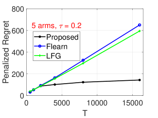
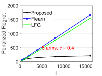
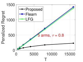
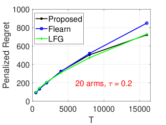
Setting 1. We investigate the relationship between cumulative penalized regret and total time horizon ($T$) under three algorithms (proposed method, LFG, and Flearn). The parameters are constructed as follows. The number of arms ($K$) is set to be 5 or 20. The total time horizon ($T$) varies from 500 to 16000. The fairness proportion $\tau_{k}$ of each arm is set to be $\tau_{k}=\tau/K$ with $\tau\in\{0.2,0.4,0.8\}$. The penalty rate $A_{k}$ is constructed as $A_{k}\equiv(\max_{k}\mu_{k}-\min_{k}\mu_{k})/2$. Each entry of the mean reward vector $(\mu_{k})$ is randomly generated between $[0,1]$. The reward distribution of each arm is a Gaussian distribution, e.g., $N(\mu_{k},\frac{1}{K^{2}})$. For Flearn algorithm, we take tuning parameter $\alpha=0$. For LFG algorithm, we take $\eta_{0}=\sqrt{T}$. Each case is replicated for 50 times.

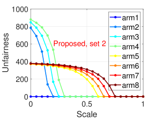
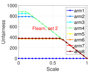
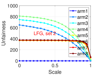
Setting 2. We investigate the path of unfairness level ($(\tau_{k}T-N_{k}(T))_{+}$) of each arm when the tuning parameter varies. The parameters of two cases are constructed as follows.

Case 1: $K=8,T=10000$; $(\mu_{1},\ldots,\mu_{8})=(0.9,0.7,0.6,0.5,0.4,0.3,0.2,0.1)$; $\tau_{1}=\ldots=\tau_{8}=\frac{1}{2K}$. The reward distribution of each arm is a Gaussian distribution, e.g., $N(\mu_{k},\frac{1}{K^{2}})$.

Case 2: $K=8,T=10000$; $(\mu_{1},\ldots,\mu_{8})=(0.95,0.7,0.65,0.6,0.2,0.15,0.1,0.05)$; $\tau_{1}=\ldots=\tau_{4}=0.8\frac{1}{K}$ and $\tau_{5}=\ldots=\tau_{8}=0.4\tau_{1}$. Again, the reward distribution of each arm is $N(\mu_{k},\frac{1}{K^{2}})$.

The penalty rates $A_{k}\equiv\eta$, where we call $\eta$ is the scale parameter which takes value between 0 and 1. For Flearn algorithm, the tuning parameter $\alpha=(1-\eta)\tau_{1}T$ with $\eta$ varying from 0 to 1. For LFG algorithm, the tuning parameter $\eta_{0}=(1-\eta)T$ with $\eta\in(0,1]$. When scale parameter $\eta\rightarrow 1$, three algorithms will prefer to exploit the arm with highest reward and pay less attention to the fairness. On the other hand, $\eta\rightarrow 0$, three algorithms tend to treat the fairness as the priority.

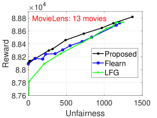
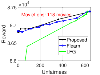
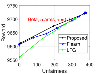
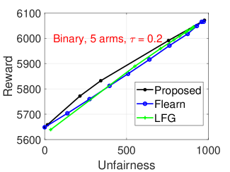
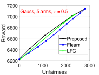
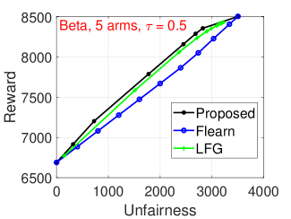
Setting 3. We investigate the relationship between total expected reward ($\sum_{t=1}^{T}\mu_{\pi_{t}}$) and unfairness level ($\sum_{k\in[K]}(\tau_{k}T-N_{k}(T))_{+}$) for three algorithms by utilizing MoiveLens 1M data set . It contains one million ratings from 6000 users on 4000 movies with each rating taking discrete values in $\{1,2,3,4,5\}$. The procedure for pre-processing the dataset are described as follows. We extract those movies with number of rating records greater than $m_{0}$. For each of remaining movies, we view it as an action and we can compute its empirical rating probability as the corresponding reward distribution (i.e., five-category distribution). Different values of $m_{0}$ are considered in our experiments, specifically, $m_{0}\in\{2500,2000,1250\}$. As a result, there are 13, 31 and 118 actions (movies), respectively.

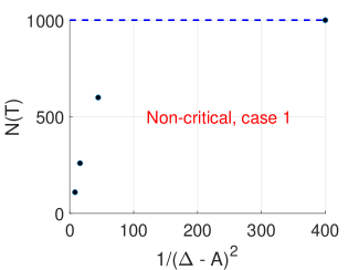
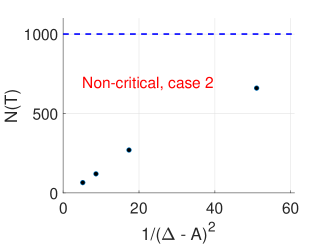
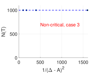
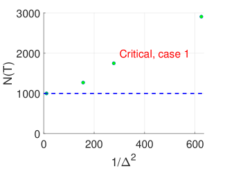
Setting 4. Moreover, we examine the relationship between number of times that non-critical arm $k$ has been pulled at $T$ (=20000) rounds and the inverse gap $1/(\Delta_{k}-A_{k})^{2}$. In particular, we construct the following three parameter settings ($\tau_{k}\equiv 1/20$) with $K=9$ arms.

Case 1: $\bm{\mu}=(0.9,0.8,0.7,0.6,0.6,0.4,0.3,0.2,0.1)$; $A_{k}\equiv 0.45$.

Case 2: $\bm{\mu}=(0.95,0.8,0.7,0.6,0.6,0.4,0.3,0.2,0.1)$; $A_{k}\equiv 0.41$.

Case 3: $\bm{\mu}=(0.9,0.8,0.7,0.6,0.6,0.425,0.4,0.375,0.35)$; $A\equiv 0.45$.

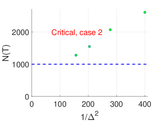
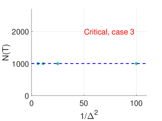
Similarly, we examine the relationship between number of times that critical arm $k$ has been pulled at $T$ (=20000) rounds and the inverse gap $1/\Delta_{k}^{2}$. We set $K=9$, $\tau_{k}\equiv 1/20$, $A_{k}\equiv 0.45$.

Case 1: $\bm{\mu}=(0.9,0.86,0.84,0.82,0.6,0.4,0.3,0.2,0.1)$.

Case 2: $\bm{\mu}=(0.9,0.85,0.84,0.83,0.82,0.4,0.3,0.2,0.1)$.

Case 3: $\bm{\mu}=(0.9,0.8,0.7,0.6,0.5,0.4,0.3,0.2,0.1)$.

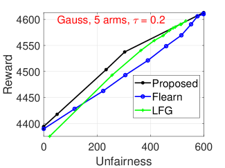
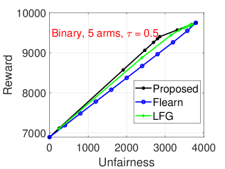
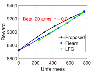
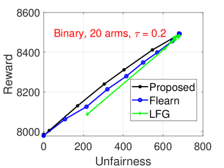
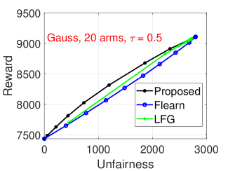
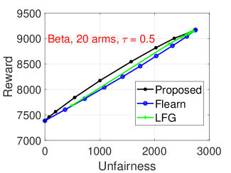
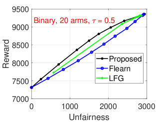
Setting 5. We additionally investigate the relationship between total expected reward ($\sum_{t=1}^{T}\mu_{\pi_{t}}$) and unfairness level ($\sum_{k\in[K]}(\tau_{k}T-N_{k}(T))_{+}$) for three algorithms under various choices of tuning parameter. The parameters are given as follows. We set $K\in\{5,20\}$ and $\tau_{k}\equiv\tau/K$ with $\tau\in\{0,20.5\}$. Each element in mean reward vector $(\mu_{k})$ is generated between 0 and 1. Moreover, we generate the reward from three different distributions, (i) Gaussian $N(\mu_{k},\frac{1}{K^{2}})$, (ii) Beta $Beta(\mu_{k},1-\mu_{k})$, (iii) Bernoulli $Bern(1,\mu_{k})$.

6.2 Result Interpretations

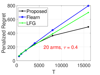
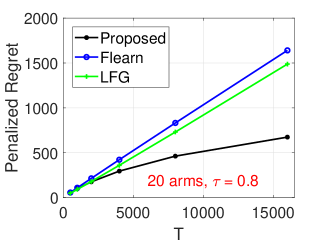
From Figure 1, we observe that the proposed method achieves smaller penalized regret compared with LFG and Flearn. This confirms that our method is indeed a good learning algorithm under penalization framework.

Figure 1: Penalized Regret ($R_{\pi}(T)$) vs Different Time Horizon ($T$) under Setting 1 of different parameters.

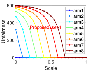
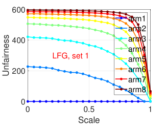
From Figure 2, it can be seen that the paths of unfairness level show different behaviors under three algorithms. For our method, with scale parameter decreasing, each arm becomes unfair one by one. By contrast, all arms under both Flearn and LFG methods suddenly become unfair once scale parameter decreases from one. This suggests that our method has sparsity feature as LASSO does, i.e., making arms with small sub-optimality gap fair. Therefore, our method can be incorporated into a sparse learning problem for choosing the subset of best arms.

Figure 2: Unfairness path ($(\tau_{k}T-N_{k}(T))_{+}$, $k\in[K]$) for three algorithms under two settings described in experiment of Setting 2. (Upper row is for Case 1 and bottom row is for Case 2.) For sub-optimal arms, the proposed method can guarantee the fairness with a wider range of tuning parameter. By contrast, Flearn and LFG can break the fairness easily.

From Figure 3, we can tell that the proposed method always achieves the highest reward given the same unfairness level for the MovieLens dataset with different number of movies. This gives the evidence that hard-threshold UCB algorithm makes better balance between total reward and fairness constraints compared with other competing methods.

Figure 3: Total reward vs unfairness level for three algorithms under different settings based on MoiveLens dataset.

From Figure 4, we can see that the pulling number $N_{k}(T)$ is proportional to $1/(\Delta_{k}-A_{k})^{2}$ for $k\in\mathcal{A}_{\text{non-cr}}$ when $N_{k}(T)$ does not reach fairness level $\tau_{k}T$. We also see that $N_{k}(T)$ is proportional to $1/\Delta_{k}^{2}$ for $k\in\mathcal{A}_{\text{cr}}$ when the pulling number is larger than fairness level $\tau_{k}T$. These phenomena match the regret bound obtained in Theorem 4.2 and empirically validate the tightness of our theoretical analysis.

The relationship between total expected reward ($\sum_{t=1}^{T}\mu_{\pi_{t}}$) and unfairness level ($\sum_{k\in[K]}(\tau_{k}T-N_{k}(T))_{+}$) for three algorithms are illustrated in Figure 5. All results confirm that our proposed method is superior in balancing between cumulative rewards and fairness requirements.

Figure 4: Upper row: $N_{k}(T)$ vs $1/(\Delta_{k}-A_{k})^{2}$ for arm $k\in\mathcal{A}_{\text{non-cr}}$. Bottom row: $N_{k}(T)$ vs $1/\Delta_{k}^{2}$ for arm $k\in\mathcal{A}_{\text{cr}}$. In all plots, the blue horizontal line stands for fairness level $\tau_{k}T$.

7 Conclusion

In this paper, we provide a new framework of MAB problems by introducing regularization terms. The advantage of our new approach is that it allows the user to distinguish between arms for which is more important to sample an arm with required frequency level and arms for which it is less important to do so. A hard-threshold UCB algorithm is proposed and has been shown to have good performance under this framework. Unlike other existing algorithms, the proposed algorithm not only achieves the asymptotic fairness but also handles well in balancing between reward and fairness constraints. A relatively complete theory, including both gap-dependent / independent upper and lower bounds, has been established. Our new theoretical results significantly contribute to the bandit problems in machine learning field and bring better insights in how to play smartly in the exploitation and exploration games.

Figure 5: Total reward vs unfairness level for three algorithms under different generation mechanisms as described in Setting 5. (The first row is for 5 arms with required fraction of times $\tau=0.2$; The second row is for 5 arms with required fraction of times $\tau=0.5$; The third row is for 20 arms with required fraction of times $\tau=0.2$; The fourth row is for 20 arms with required fraction of times $\tau=0.5$. The first column is for Gaussian reward distribution; the second column is for Beta distribution; and the third column is for Bernoulli distribution.) Given the fixed unfairness level, the proposed method can have larger total reward than other two methods consistently over all experimental settings.

Overview of Appendix

We collect all technical proofs in this appendix. Specifically, the proofs of gap-dependent upper and lower bounds are given in Section A and B. The proofs of gap independent upper and lower bounds are given in Section D and E, respectively. The proof of $\mathbb{E}[\max_{1\leq t\leq T}(\tau_{k}t-N_{k}(t))]_{+}$ is given in Section C.

Appendix A Proof of Gap-dependent Upper Bounds

Proof of Theorem 4.1 Its proof is essentially same as the proof of first part in Theorem 4.2 by treating the non-critical set $\mathcal{A}_{\text{non-cr}}$ empty.

Proof of Theorem 4.2 We first prove the first part: $\mathbb{E}[(\tau_{k}T-N_{k}(T))_{+}]=O(1)$ for any $k\in\mathcal{A}_{\text{opt}}\cup\mathcal{A}_{\text{cr}}$.

Suppose at time $n$ that a critical arm $k$ is played less than $\tau_{k}n$. We can prove that the algorithm pulls critical arm $k^{\prime}$ at time $n$ such that $N_{k^{\prime}}(n)\geq 8\log T/c_{a}^{2}$ and $N_{k^{\prime}}(n)>\tau_{k}n$ with vanishing probability. This is because

$$\mathbb{P}(A_{k}+m_{k}(n)+\sqrt{\frac{2\log n}{N_{k}(n)}}\leq m_{k^{\prime}}(n)+\sqrt{\frac{2\log n}{N_{k^{\prime}}(n)}})$$ (15)

$$\leq \mathbb{P}(A_{k}+\mu_{k}\leq+\mu_{k}^{\prime}+2\sqrt{\frac{2\log n}{N_{k^{\prime}}(n)}})+\frac{2}{n^{2}}$$

$$\leq \mathbb{P}(A_{k}-\Delta_{k}\leq-\Delta_{k^{\prime}}+2\sqrt{\frac{2\log n}{N_{k^{\prime}}(n)}})+\frac{2}{n^{2}}$$

$$= 2/n^{2}.$$

By the same reason, the algorithm pulls non-critical arm $k^{\prime\prime}$ at time $n$ when $N_{k^{\prime\prime}}(n)\geq 8\log T/c_{a}^{2}$ with vanishing probability.

(Observation 3) In other words, it holds with high probability that once a critical arm $k$ is played with proportion less than required level $\tau_{k}$’s, it must be pulled in next round when all other arms is played with proportion greater than level $\tau_{k}$’s and is played more than $8\log T/c_{a}^{2}$ times.

(Observation 4) It also holds with high probability that once a non-critical arm is played more than $8\log T/c_{a}^{2}$, it can be only played when all critical arms are played with frequency more than the required level $\tau_{k}$’s.

Moreover, we can show that $N_{k^{\prime}}(n)\geq 8\log T/c_{a}^{2}$ at time $n=c_{0}T/2$ for each critical arm $k^{\prime}$. If not, note that $8\log T/c_{a}^{2}\leq\tau_{k^{\prime}}c_{0}T/4$, then $N_{k}^{\prime}(n)<\tau_{k}^{\prime}n$ for any $n\in\{\lceil c_{0}T/4\rceil,\ldots,\lfloor c_{0}T/2\rfloor\}$. Hence, for any critical arm $k^{\prime}$ can be played at most $\max\{\tau_{k^{\prime}}c_{0}T/4,8\log T/c_{a}^{2}\}$ times between rounds $c_{0}T/2$ and $c_{0}T$; every non-critical arm $k^{\prime\prime}$ can be played at most $8\log T/c_{a}^{2}$ times. Then, we must have

$$c_{0}T/2-c_{0}T/4\leq\sum_{k}\tau_{k}c_{0}T/4+\sum_{k}8\log T/c_{a}^{2}.$$

However, the above inequality fails to hold when $T/\log T\geq 16c_{0}^{2}K/c_{a}^{2}$. This leads to the contradiction. Thus, we have $N_{k^{\prime}}(n)\geq 8\log T/c_{a}^{2}$ for any critical arm $k^{\prime}$ at time $n=c_{0}T/2$.

Actually, this further gives us that we must have $N_{k^{\prime}}(n)\geq\lfloor\tau_{k^{\prime}}n\rfloor$ for all critical arms at some time $n\in[c_{0}T/2,T]$. To see this, we observe the fact that for any arm $\bar{k}$, it will be played with probability less than $\frac{2}{T^{2}}$ at time $n$ once $N_{\bar{k}}(n)\geq\max\{\tau_{k}n,8\log T/c_{a}^{2}\}$ and one critical arm $k^{\prime}$ is played less than $\tau_{k^{\prime}}n$. (In other words, this tells us that once arm $\bar{k}$ has been played $\max\{\tau_{\bar{k}}n,8\log T/c_{a}^{2}\}$ times, then it can only be played at time when all critical arms $k^{\prime}$s have been played for $\tau_{k^{\prime}}n$ times or $\lfloor\tau_{\bar{k}}n\rfloor$ jumps by one with probability greater than $1-2/T^{2}$.)

Let $n_{1}(\geq c_{0}T/2)$ be the first ever time such that $N_{k^{\prime}}(n_{1})\geq\lfloor\tau_{k^{\prime}}n_{1}\rfloor$ for all critical arms $k^{\prime}$s. By straightforward calculation, it gives that $n_{1}$ must be bounded by

$$n_{1}\leq c_{0}T/2+\sum_{k:\text{non-critical}}8\log T/c_{a}^{2}+(\sum_{k:\text{critical}}\tau_{k})T$$

with probability greater than $1-2K/T$. That is, $n_{1}$ is well defined between $c_{0}T/2$ and $T$. At time $n_{1}$, we have all critical arms $k^{\prime}$ such that $N_{k^{\prime}}(n_{1})\geq\tau_{k^{\prime}}n_{1}$.

Moreover, we consider the first time $n_{2}(>n_{1})$ such that every non-critical arm $k^{\prime\prime}$ has been played for at least $8\log T/c_{a}^{2}$ times when $\Delta_{k^{\prime\prime}}-A_{k^{\prime\prime}}\leq c_{a}\sqrt{\frac{\log(c_{0}T/2)}{16\log T}}$ (which is asymptotically $c_{a}/4$). We claim that $n_{2}\leq n_{1}+c_{0}T/2$. This is because, between rounds $n_{1}$ and $n_{2}$, the algorithm will choose non-critical arm $k^{\prime\prime}$ when $N_{k^{\prime}}(n)\geq\tau_{k^{\prime}}(n)$ for all critical arms $k^{\prime}$s and $N_{k^{\prime\prime}}(n)\leq\min\{\log(c_{0}T/2)/2(\Delta_{k^{\prime\prime}}-A_{k^{\prime\prime}})^{2},\tau_{k^{\prime\prime}}c_{0}T/2\}$. To see this, we know that

$$\mathbb{P}(m_{k^{\prime}}(n)+\sqrt{\frac{2\log n}{N_{k^{\prime}}(n)}}\geq m_{k^{\prime\prime}}(n)+A_{k^{\prime\prime}}+\sqrt{\frac{2\log n}{N_{k^{\prime\prime}}(n)}})$$ (16)

$$\leq \mathbb{P}(\mu_{k}^{\prime}+2\sqrt{\frac{2\log n}{N_{k^{\prime}}(n)}}\geq\mu_{k^{\prime\prime}}+A_{k^{\prime\prime}}+\sqrt{\frac{\log n}{N_{k^{\prime\prime}}(n)}})+2/n$$

$$\leq \mathbb{P}(\mu_{k}^{\prime}+2\sqrt{\frac{2\log T}{\tau_{k^{\prime}}c_{0}T/2}}\geq\mu_{k^{\prime\prime}}+A_{k^{\prime\prime}}+\sqrt{\frac{\log(c_{0}T/2)}{N_{k^{\prime\prime}}(n)}})+2/n$$

$$\leq \mathbb{P}(\Delta_{k^{\prime\prime}}-A_{k^{\prime\prime}}+2\sqrt{\frac{2\log T}{\tau_{k^{\prime}}c_{0}T/2}}\geq\sqrt{\frac{\log(c_{0}T/2)}{N_{k^{\prime\prime}}(n)}})+2/n$$

$$\leq \mathbb{P}(\Delta_{k^{\prime\prime}}-A_{k^{\prime\prime}}\geq\sqrt{\frac{\log(c_{0}T/2)}{2N_{k^{\prime\prime}}(n)}})+2/n$$

$$\leq 4/c_{0}T.$$

for $n\geq c_{0}T/2$. That is, index of arm $k^{\prime\prime}$ is larger than $k^{\prime}$ with high probability.

In other words, for each round between $n_{1}$ and $n_{2}$, each critical arm $k^{\prime}$ can be only pulled at most $\tau_{k^{\prime}}(n_{2}-n_{1})$ before every non-critical arm $k^{\prime\prime}$ has been played for $\min\{8\log T/c_{a}^{2},\log(c_{0}T/2)/2(\Delta_{k^{\prime\prime}}-A_{k^{\prime\prime}})^{2}\}$ ($\equiv 8\log T/c_{a}^{2}$ when $\Delta_{k^{\prime\prime}}-A_{k^{\prime\prime}}<c_{a}/4$). Additionally, each non-critical arm $k^{\prime\prime}$ can be only played for at most $8\log T/(\Delta_{k}-A_{k})^{2}$ with high-probability. Therefore, it must hold that

$$n_{2}-n_{1}\leq(\sum_{k}\tau_{k})(n_{2}-n_{1})+\sum_{k}8\log T/(\Delta_{k}-A_{k})^{2}.$$

However, the above inequality fails to hold when $n_{2}-n_{1}\geq c_{0}T/2$ under assumption that $\Delta_{k}-A_{k}\geq\sqrt{\frac{8K\log T}{c_{0}^{2}T}}$. This validates the claim $n_{2}\leq n_{1}+c_{0}T/2$.

Starting from time $n_{2}$, by the observations 3 and 4, it can be seen that the maximum values of $(\tau_{k^{\prime}}n-N_{k^{\prime}}(n))_{+}$ for any critical arm $k^{\prime}$ is always bounded by 1 with probability $1-2K/T$ ($n\in[n_{2},T]$). This completes the proof of the first part.

For the second part, we need to prove $\mathbb{E}[N_{k}(T)]\leq\max\{\frac{8\log T}{\Delta_{k}^{2}},\tau_{k}T\}+O(1)$ for $k\in\mathcal{A}_{\text{cr}}$.

When $\frac{8\log T}{\Delta_{k}^{2}}>\tau_{k}T$, we can calculate the probability

$$\mathbb{P}(\textrm{arm $k$ is pulled at round $n+1$}~{}|N_{k}(n)\geq\frac{8\log T}{\Delta_{k}^{2}})$$ (17)

$$\leq \mathbb{P}(i_{k}(n+1)\geq i_{k^{\ast}}(n+1))$$

$$\leq \mathbb{P}(\hat{m}_{k}(n+1)+\sqrt{\frac{2\log(n+1)}{N_{k}(n)}}\geq\hat{m}_{k^{\ast}}(n+1)+\sqrt{\frac{2\log(n+1)}{N_{k}(n)}})$$

$$\leq 1/n^{2}\leq 1/(8\log T/\Delta_{k})^{2}\leq 1/(\tau_{k}T)^{2}.$$

When $\frac{8\log T}{\Delta_{k}^{2}}\leq\tau_{k}T$, we can similarly calculate the probability

$$\mathbb{P}(\textrm{arm $k$ is pulled at round $n+1$}~{}|N_{k}(n)\geq\tau_{k}T)$$ (18)

$$\leq \mathbb{P}(i_{k}(n+1)\geq i_{k^{\ast}}(n+1))$$

$$\leq \mathbb{P}(\hat{m}_{k}(n+1)+\sqrt{\frac{2\log(n+1)}{N_{k}(n)}}\geq\hat{m}_{k^{\ast}}(n+1)+\sqrt{\frac{2\log(n+1)}{N_{k}(n)}})$$

$$\leq 1/n^{2}\leq 1/(\tau_{k}T)^{2}.$$

Hence we can easily obtain that $\mathbb{E}[N_{k}(T)]\leq\max\{\frac{8\log T}{\Delta_{k}^{2}},\tau_{k}T\}+O(1)$ by union bound.

For the third part that $\mathbb{E}[N_{k}(T)]\leq\min\{\frac{8\log T}{(\Delta_{k}-A_{k})^{2}},\tau_{k}T\}+O(1)$ ($k_{j}\in\mathcal{A}_{\text{non-cr}}$), it follows from the fact that we can treat $\mu_{k}+A_{k}$ as new expected reward for arm $k\in\mathcal{A}_{\text{non-cr}}$. Thus the corresponding sub-optimality gap is $\Delta_{k}-A_{k}$. The result follow by using standard technique in the classical UCB algorithm. Hence we omit the details here.

Finally, by combining three parts and straightforward calculation, we obtain the desired gap-dependent upper bounds. This concludes the proof.

Appendix B Proof of Gap-dependent Lower Bounds

Proof of Theorem 4.6.  We consider the following setting, where arm 1 is the optimal arm with a deterministic reward $\Delta$ and arms $k$, $(k\geq 2)$ are sub-optimal arms with reward zero. Let penalty rate $A_{k}=A$ for all $k\in[K]$ with $\Delta>A$. Assuming that $\frac{8\log T}{(\Delta-A)^{2}}\leq\tau_{k}T/2$, we construct a lower bound as follows.

We claim that each arm $k\geq 2$ will be played at least $n_{1}:=\frac{\log T}{(\Delta-A)^{2}}$ times. If there exists an arm $k_{0}$ has not been played for $n_{1}$ times, we then consider the time index $n_{a}=T/2+1+(K-2)\frac{8\log T}{(\Delta-A)^{2}}+n_{1}$. At this time, we have that arm $1$ is the arm with largest index since that for each sub-optimal arm $k\neq k_{0}$, its index will never exceeds $\Delta$ once it has been played $\frac{8\log T}{(\Delta-A)^{2}}$ times. According to assumption that arm $k_{0}$ has been played less than $n_{1}$ times, thus arm 1 is the arm with largest index at time $n_{a}$.

However, the index of arm 1 at time $n_{a}$ is never larger than $\sqrt{\frac{2\log T}{T/2}}+\Delta$. The index of arm $k_{0}$ at time $n_{a}$ is always larger than $A+\sqrt{\frac{2\log(T/2)}{n_{1}}}$. It gives

$$i_{1}(n_{a})\leq\sqrt{\frac{2\log T}{T/2}}+\Delta<A+\sqrt{\frac{2\log(T/2)}{n_{1}}}\leq i_{k_{0}}(n_{a}),$$ (19)

which leads to the contradiction of the mechanism of the proposed algorithm. Hence, we have that each sub-optimal should have been played for at least $\frac{\log T}{(\Delta-A)^{2}}$ times.

Proof of Theorem 4.7.  We consider another setting, where arm 1 is the optimal arm with deterministic reward $\Delta_{1}+\Delta_{2}$, arm $k$’s $(k\in\mathcal{A}_{cr})$ are sub-optimal arms with reward being $\Delta_{1}$ and arm $k$’s $(k\in\mathcal{A}_{non-cr})$ ar sub-optimal arms with reward being $\Delta_{2}$. Let penalty rate $A_{k}=A_{2}$ for all $k\in\mathcal{A}_{cr}$ with $\Delta_{2}<A_{2}$ and penalty rate $A_{k}=A_{1}$ for all $k\in\mathcal{A}_{non-cr}$ with $\Delta_{1}>A_{1}$. Assume that $\sum_{k\in\mathcal{A}_{non-cr}}\frac{8\log T}{(\Delta_{1}-A_{1})^{2}}+\sum_{k\in\mathcal{A}_{cr}}\frac{8\log T}{\Delta_{2}^{2}}<T/2$ and $\tau_{k}T\leq\frac{\log T}{\Delta_{2}^{2}}$ for $k\in\mathcal{A}_{cr}$, we then have the following lower bound.

We claim that for each arm $k\in\mathcal{A}_{cr}$ will be played for at least $n_{2}:=\frac{\log T}{\Delta_{2}^{2}}$ times. If not, there will be at least one arm $k_{1}\in\mathcal{A}_{cr}$ has been played for less than $n_{2}$ times. We consider the time stamp, $n_{b}=T/2+1+\sum_{k\in\mathcal{A}_{non-cr}}\frac{8\log T}{(\Delta_{1}-A_{1})^{2}}+\sum_{k\in\mathcal{A}_{cr};k\neq k_{1}}\frac{8\log T}{\Delta_{2}^{2}}+n_{2}$. At this time, we have that arm 1 is the arm with the largest index since that for each arm in $\mathcal{A}_{non-cr}$, its index is always smaller than $\Delta_{1}+\Delta_{2}$ once it has been played for $\frac{8\log T}{(\Delta_{1}-A_{1})^{2}}$ times. For each arm $k\in\mathcal{A}_{cr}$ ($k\neq k_{1}$), its index is also smaller than $\Delta_{1}+\Delta_{2}$ once it has been played for $\frac{8\log T}{\Delta_{2}^{2}}$ times. According to assumption that arm $k_{1}$ has been played less than $n_{2}$ times, thus arm 1 is the arm with largest index at time $n_{b}$.

However, on other hand, the index of arm 1 at time $n_{b}$ is never larger than $\sqrt{\frac{2\log T}{T/2}}+\Delta_{1}+\Delta_{2}$. The index of arm $k_{1}$ is not smaller than $\Delta_{1}+\sqrt{\frac{2\log(T/2)}{n_{2}}}$. It leads to

$$i_{1}(n_{b})\leq\sqrt{\frac{2\log T}{T/2}}+\Delta_{1}+\Delta_{2}\leq\Delta_{1}+\sqrt{\frac{2\log(T/2)}{n_{2}}}\leq i_{2}(n_{b}),$$

this contradicts with arm 1 is arm with largest index at time $n_{b}$. Hence, any arm in $\mathcal{A}_{cr}$ should be played at least $\frac{\log T}{\Delta_{2}^{2}}$ times.

Appendix C Proof of Maximal Inequality (Proof of Theorem 4.3)

We can order $K$ arms according to the sums $\mu_{k}+A_{k}$’s. Specifically, let the order $k_{1},k_{2},\ldots,k_{K}$ be defined by

$$\mu_{k_{1}}+A_{k_{1}}>\mu_{k_{2}}+A_{k_{2}}>\cdots>\mu_{k_{K}}+A_{k_{K}}.$$ (20)

For simplicity we assume no ties in (20). We also assume that $A_{k}>\Delta_{k}$ for all $k\in\mathcal{A}_{\rm opt}\cup\mathcal{A}_{\rm cr}$.

We now aim to bound expectations of the $\mathbb{E}\max_{t\in[T]}\bigl{(}\tau_{k}t-N_{k}(t)\bigr{)}_{+}$ for $k\in\mathcal{A}_{\rm opt}\cup\mathcal{A}_{\rm cr}$. We will use the ordering of the arms $k_{1},k_{2},\ldots,k_{K}$ defined in (20). Take any arbitrary $t\in[T]$ and let $k_{j}\in\mathcal{A}_{\rm opt}\cup\mathcal{A}_{\rm cr}$,

$$m_{t}^{(j)}=\sup\bigl{\{}n=1,\ldots,t:\,\tau_{k_{j}}n\leq N_{k_{j}}(n)\bigr{\}}.$$ (21)

Suppose for a moment that $m_{t}^{(j)}<t$. We have

$$\bigl{(}\tau_{k_{j}}t-N_{k_{j}}(t)\bigr{)}_{+}\leq\tau_{k_{j}}$$ (22)

$$+ \tau_{k_{j}}\#\bigl{\{}n=m_{t}^{(j)}+1,\ldots,t:\,\tau_{k_{d}}n>N_{k_{d}}(n-1)\ \text{for some}\ d=1,\ldots,j-1\bigr{\}}$$

$$+ \tau_{k_{j}}\#\bigl{\{}n=m_{t}^{(j)}+1,\ldots,t:\,\tau_{k_{d}}n\leq N_{k_{d}}(n-1)\ \text{for all}\ d=1,\ldots,j-1,$$

$$\hskip 224.03743pt\text{arm $k_{j}$ not pulled at time $n$}\bigr{\}}$$

$$- (1-\tau_{k_{j}})\#\bigl{\{}n=m_{t}^{(j)}+1,\ldots,t:\,\tau_{k_{d}}n\leq N_{k_{d}}(n-1)\ \text{for all}\ d=1,\ldots,j-1,$$

$$\hskip 224.03743pt\text{arm $k_{j}$ pulled at time $n$}\bigr{\}}$$

$$= \tau_{k_{j}}+\tau_{k_{j}}\#\bigl{\{}n=m_{t}^{(j)}+1,\ldots,t:\,\tau_{k_{d}}n>N_{k_{d}}(n-1)\ \text{for some}\ d=1,\ldots,j-1\bigr{\}}$$

$$- (1-\tau_{k_{j}})\#\bigl{\{}n=m_{t}^{(j)}+1,\ldots,t:\,\tau_{k_{d}}n\leq N_{k_{d}}(n-1)\ \text{for all}\ d=1,\ldots,j-1\bigr{\}}$$

$$+ \#\bigl{\{}n=m_{t}^{(j)}+1,\ldots,t:\,\tau_{k_{d}}n\leq N_{k_{d}}(n-1)\ \text{for all}\ d=1,\ldots,j-1,$$

$$\hskip 224.03743pt\text{arm $k_{j}$ not pulled at time $n$}\bigr{\}}$$

$$= \tau_{k_{j}}+\#\bigl{\{}n=m_{t}^{(j)}+1,\ldots,t:\,\tau_{k_{d}}n>N_{k_{d}}(n-1)\ \text{for some}\ d=1,\ldots,j-1\bigr{\}}$$

$$+ \#\bigl{\{}n=m_{t}^{(j)}+1,\ldots,t:\,\tau_{k_{d}}n\leq N_{k_{d}}(n-1)\ \text{for all}\ d=1,\ldots,j-1,$$

$$\hskip 224.03743pt\text{arm $k_{j}$ not pulled at time $n$}\bigr{\}}$$

$$- {(1-\tau_{k_{j}})(t-m_{t}^{(j)})}.$$

The final bound is, clearly, also valid in the case $m_{t}^{(j)}=t$.

Next,

$$\#\bigl{\{}n=m_{t}^{(j)}+1,\ldots,t:\,\tau_{k_{d}}n>N_{k_{d}}(n-1)\ \text{for some}\ d=1,\ldots,j-1\bigr{\}}$$ (23)

$$=\sum_{d=1}^{j-1} \#\bigl{\{}n=m_{t}^{(j)}+1,\ldots,t:\,\tau_{k_{d}}n>N_{k_{d}}(n-1),\,\tau_{k_{m}}n\leq N_{k_{m}}(n-1),\,m=1,\ldots,d-1\bigr{\}}.$$

For $d=1,\ldots,j-1$ denote

$$m_{t}^{(j,d)}=\sup\bigl{\{}n=m_{t}^{(j)},\ldots,t:\,\tau_{k_{d}}n>N_{k_{d}}(n-1)\bigr{\}}.$$ (24)

Suppose, for a moment, that $m_{t}^{(j,d)}>m_{t}^{(j)}$. Then

$$0<\tau_{k_{d}}m_{t}^{(j,d)}- N_{k_{d}}\bigl{(}m_{t}^{(j,d)}-1\bigr{)}=\tau_{k_{d}}m_{t}^{(j)}-N_{k_{d}}\bigl{(}m_{t}^{(j)}-1\bigr{)}$$

$$+ \tau_{k_{d}}\Bigl{(}m_{t}^{(j,d)}-m_{t}^{(j)}-\#\bigl{\{}n=m_{t}^{(j)}+1,\ldots,m_{t}^{(j,d)}:\ \text{arm $k_{d}$ pulled}\bigr{\}}\Bigr{)}$$

$$- (1-\tau_{k_{d}})\#\bigl{\{}n=m_{t}^{(j)}+1,\ldots,m_{t}^{(j,d)}:\ \text{arm $k_{d}$ pulled}\bigr{\}}$$

$$= \tau_{k_{d}}m_{t}^{(j)}-N_{k_{d}}\bigl{(}m_{t}^{(j)}-1\bigr{)}+\tau_{k_{d}}\bigl{(}m_{t}^{(j,d)}-m_{t}^{(j)}\bigr{)}$$

$$- \#\bigl{\{}n=m_{t}^{(j)}+1,\ldots,m_{t}^{(j,d)}:\ \text{arm $k_{d}$ pulled}\bigr{\}}.$$

We conclude that

$$\#\bigl{\{}n=m_{t}^{(j)}+1,\ldots,m_{t}^{(j,d)}:\ \text{arm $k_{d}$ pulled}\bigr{\}}$$

$$\leq \max_{n=1,\ldots,t}\bigl{(}\tau_{k_{d}}n-N_{k_{d}}(n)\bigr{)}_{+}+\tau_{k_{d}}\bigl{(}m_{t}^{(j,d)}-m_{t}^{(j)}\bigr{)}.$$

Therefore,

$$\#\bigl{\{}n=m_{t}^{(j)}+1,\ldots,t:\,\tau_{k_{d}}n>N_{k_{d}}(n-1),\,\tau_{k_{m}}n\leq N_{k_{m}}(n-1),\,m=1,\ldots,d-1\bigr{\}}$$

$$= \#\bigl{\{}n=m_{t}^{(j)}+1,\ldots,m_{t}^{(j,d)}:\,\tau_{k_{d}}n>N_{k_{d}}(n-1),\,\tau_{k_{m}}n\leq N_{k_{m}}(n-1),\,m=1,\ldots,d-1\bigr{\}}$$

$$\leq \#\bigl{\{}n=m_{t}^{(j)}+1,\ldots,m_{t}^{(j,d)}:\ \text{arm $k_{d}$ pulled}\bigr{\}}$$

$$+ \#\bigl{\{}n=m_{t}^{(j)}+1,\ldots,t:\,\tau_{k_{d}}n>N_{k_{d}}(n-1),\,\tau_{k_{m}}n\leq N_{k_{m}}(n-1),\,m=1,\ldots,d-1,$$

$$\hskip 325.215pt\text{arm $k_{d}$ not pulled}\bigr{\}}$$

$$\leq \max_{n=1,\ldots,t}\bigl{(}\tau_{k_{d}}n-N_{k_{d}}(n)\bigr{)}_{+}+\tau_{k_{d}}\bigl{(}t-m_{t}^{(j)}\bigr{)}$$

$$+ \#\bigl{\{}n=m_{t}^{(j)}+1,\ldots,t:\,\tau_{k_{d}}n>N_{k_{d}}(n-1),\,\tau_{k_{m}}n\leq N_{k_{m}}(n-1),\,m=1,\ldots,d-1,$$

$$\hskip 325.215pt\text{arm $k_{d}$ not pulled}\bigr{\}},$$

and the final bound is clearly valid even if $m_{T}^{(j,d)}=m_{T}^{(j)}$. Substituting this bound into (23) we obtain

$$\#\bigl{\{}n=m_{t}^{(j)}+1,\ldots,t:\,\tau_{k_{d}}n>N_{k_{d}}(n-1)\ \text{for some}\ d=1,\ldots,j-1\bigr{\}}$$

$$\leq \bigl{(}t-m_{t}^{(j)}\bigr{)}\sum_{d=1}^{j-1}\tau_{k_{d}}+\sum_{d=1}^{j-1}\max_{t^{\prime}=1,\ldots,t}\bigl{(}\tau_{k_{d}}t^{\prime}-N_{k_{d}}(t^{\prime})\bigr{)}_{+}$$

$$+ \sum_{d=1}^{j-1}\#\bigl{\{}n=m_{t}^{(j)}+1,\ldots,t:\,\tau_{k_{d}}n>N_{k_{d}}(n-1),\,\tau_{k_{m}}n\leq N_{k_{m}}(n-1),\,m=1,\ldots,d-1,$$

$$\hskip 325.215pt\text{arm $k_{d}$ not pulled}\bigr{\}},$$

Substituting this bound into (22) gives us

$$\bigl{(}\tau_{k_{j}}t-N_{k_{j}}(t)\bigr{)}_{+}\leq\tau_{k_{j}}$$ (25)

$$+ \sum_{d=1}^{j-1}\max_{t^{\prime}=1,\ldots,t}\bigl{(}\tau_{k_{d}}t^{\prime}-N_{k_{d}}(t^{\prime})\bigr{)}_{+}-\bigl{(}t-m_{t}^{(j)}\bigr{)}\left(1-\sum_{d=1}^{j}\tau_{k_{d}}\right)$$

$$+ \sum_{d=1}^{j}\#\bigl{\{}n=m_{t}^{(j)}+1,\ldots,t:\,\tau_{k_{d}}n>N_{k_{d}}(n-1),$$

$$\hskip 72.26999pt\tau_{k_{m}}n\leq N_{k_{m}}(n-1),\,m=1,\ldots,d-1,\ \text{arm $k_{d}$ not pulled}\bigr{\}}$$

$$\leq \tau_{k_{j}}+\sum_{d=1}^{j-1}\max_{t^{\prime}=1,\ldots,t}\bigl{(}\tau_{k_{d}}t^{\prime}-N_{k_{d}}(t^{\prime})\bigr{)}_{+}$$

$$+ \sum_{d=1}^{j}\#\bigl{\{}n=1,\ldots,t:\,\tau_{k_{d}}n>N_{k_{d}}(n-1),$$

$$\hskip 72.26999pt\tau_{k_{m}}n\leq N_{k_{m}}(n-1),\,m=1,\ldots,d-1,\ \text{arm $k_{d}$ not pulled}\bigr{\}}.$$

Taking the maximum over $t$ on both sides of above inequality, we then have

$$\max_{t=1,\ldots,T}\bigl{(}\tau_{k_{j}}t-N_{k_{j}}(t)\bigr{)}_{+}\leq\tau_{k_{j}}+\sum_{d=1}^{j-1}\max_{t=1,\ldots,T}\bigl{(}\tau_{k_{d}}t-N_{k_{d}}(t)\bigr{)}_{+}$$ (26)

$$+ \sum_{d=1}^{j}\#\bigl{\{}n=1,\ldots,T:\,\tau_{k_{d}}n>N_{k_{d}}(n-1),$$

$$\hskip 72.26999pt\tau_{k_{m}}n\leq N_{k_{m}}(n-1),\,m=1,\ldots,d-1,\ \text{arm $k_{d}$ not pulled}\bigr{\}}.$$

Therefore, we arrive at

$$\mathbb{E}\left(\max_{t=1,\ldots,T}\bigl{(}\tau_{k_{j}}t-N_{k_{j}}(t)\bigr{)}_{+}\right)$$ (27)

$$\leq \tau_{k_{j}}+\mathbb{E}\left(\sum_{d=1}^{j-1}\max_{t=1,\ldots,T}\bigl{(}\tau_{k_{d}}t-N_{k_{d}}(t)\bigr{)}_{+}\right)$$

$$+ \sum_{d=1}^{j}\mathbb{E}\biggl{(}\sum_{n=1}^{T}\mathbf{1}\bigl{(}\tau_{k_{d}}n>N_{k_{d}}(n-1),$$

$$\hskip 72.26999pt\tau_{k_{m}}n\leq N_{k_{m}}(n-1),\,m=1,\ldots,d-1,\ \text{arm $k_{d}$ not pulled}\bigr{)}\biggr{)}.$$

We will prove that for $k_{d}\in\mathcal{A}_{\rm opt}\cup\mathcal{A}_{\rm cr}$

$$\mathbb{E}\biggl{(}\sum_{n=1}^{T}\mathbf{1}\bigl{(}\tau_{k_{d}}n>N_{k_{d}}(n-1),$$ (28)

$$\hskip 72.26999pt\tau_{k_{m}}n\leq N_{k_{m}}(n-1),\,m=1,\ldots,d-1,\ \text{arm $k_{d}$ not pulled}\bigr{)}\biggr{)}$$

$$\leq b_{d}\log T+O(1)$$

for $b_{d}>0$ that we will compute. It is elementary that $k_{j}\in\mathcal{A}_{\rm opt}\cup\mathcal{A}_{\rm cr}$ implies $k_{d}\in\mathcal{A}_{\rm opt}\cup\mathcal{A}_{\rm cr}$ for $d=1,\ldots,j-1$. Therefore, it will follow from (28), (27) and a simple inductive argument that for any $k_{j}\in\mathcal{A}_{\rm opt}\cup\mathcal{A}_{\rm cr}$,

$$\mathbb{E}\left(\max_{t=1,\ldots,T}\bigl{(}\tau_{k_{j}}t-N_{k_{j}}(t)\bigr{)}_{+}\right)\leq a_{j}\log T+O(1)$$ (29)

with $a_{1}=b_{1}$ and for $j>1$,

$$a_{j}=\sum_{d=1}^{j-1}a_{d}+\sum_{d=1}^{j}b_{d},$$

which means that

$$a_{j}=\sum_{d=1}^{j}(j-d+1)b_{d}.$$ (30)

We now prove (28). We have

$$E_{\pi}\biggl{(}\sum_{n=1}^{T}\mathbf{1}\bigl{(}\tau_{k_{d}}n>N_{k_{d}}(n-1),\tau_{k_{m}}n\leq N_{k_{m}}(n-1),\,m=1,\ldots,d-1,\ \text{arm $k_{d}$ not pulled}\bigr{)}\biggr{)}$$

$$= \sum_{m=1}^{d-1}E_{\pi}\biggl{(}\sum_{n=1}^{T}\mathbf{1}\bigl{(}\tau_{k_{d}}n>N_{k_{d}}(n-1),\tau_{k_{m}}n\leq N_{k_{m}}(n-1),\ \text{arm $k_{m}$ is pulled at time $n$}\bigr{)}\biggr{)}$$

$$+ \sum_{m=d+1}^{K}E_{\pi}\biggl{(}\sum_{n=1}^{T}\mathbf{1}\bigl{(}\tau_{k_{d}}n>N_{k_{d}}(n-1),\ \text{arm $k_{m}$ is pulled at time $n$}\bigr{)}\biggr{)}.$$

Observe that a “no-tie” assumption imposed at the beginning of the section implies that

$$\mu_{k_{d}}+A_{k_{d}}>\mu_{*}\geq\mu_{k_{m}}.$$

Therefore, we can use once again the usual UCB-type argument to see that for any $m=1,\ldots,d-1$, for any $B>0$,

$$E_{\pi}\biggl{(}\sum_{n=1}^{T}\mathbf{1}\bigl{(}\tau_{k_{d}}n>N_{k_{d}}(n-1),\tau_{k_{m}}n\leq N_{k_{m}}(n-1),\ \text{arm $k_{m}$ is pulled at time $n$}\bigr{)}\biggr{)}$$

$$\leq B\log T+\sum_{n=1}^{T}P_{\pi}\bigl{(}N_{k_{m}}(n-1)>B\log T,$$

$$\hskip 108.405pt\tau_{k_{d}}n>N_{k_{d}}(n-1),\tau_{k_{m}}n\leq N_{k_{m}}(n-1),\ \text{arm $k_{m}$ is pulled at time $n$}\bigr{)}$$

$$\leq B\log T+\sum_{n=1}^{T}P_{\pi}\bigl{(}N_{k_{m}}(n-1)>B\log T,$$

$$\hskip 108.405pt\tau_{k_{d}}n>N_{k_{d}}(n-1),\tau_{k_{m}}n\leq N_{k_{m}}(n-1),i_{k_{m}}(n)\geq i_{k_{d}}(n)\bigr{)}$$

$$\leq B\log T+\sum_{n=1}^{T}P_{\pi}\left(N_{k_{m}}(n-1)>B\log T,\,\hat{m}_{k_{m}}(n-1)+\sqrt{\frac{2\log n}{N_{k_{m}}(n-1)}}\right.$$

$$\left.\hskip 216.81pt\,\geq\hat{m}_{k_{d}}(n-1)+A_{k_{d}}+\sqrt{\frac{2\log n}{N_{k_{d}}(n-1)}}\right).$$

By carefully choosing

$$B=\frac{8}{(\mu_{k_{d}}+A_{k_{d}}-\mu_{k_{m}})^{2}},$$

we obtain the bound

$$E_{\pi}\biggl{(}\sum_{n=1}^{T}\mathbf{1}\bigl{(}\tau_{k_{d}}n>N_{k_{d}}(n-1),\tau_{k_{m}}n\leq N_{k_{m}}(n-1),\ \text{arm $k_{m}$ is pulled at time $n$}\bigr{)}\biggr{)}$$ (31)

$$\leq \frac{8}{(\mu_{k_{d}}+A_{k_{d}}-\mu_{k_{m}})^{2}}\log T+O(1),$$

$m=1,\ldots,d-1$. The same argument shows that for every $m=d+1,\ldots,K$,

$$E_{\pi}\biggl{(}\sum_{n=1}^{T}\mathbf{1}\bigl{(}\tau_{k_{d}}n>N_{k_{d}}(n-1),\ \text{arm $k_{m}$ is pulled at time $n$}\bigr{)}\biggr{)}$$ (32)

$$\leq \frac{8}{(\mu_{k_{d}}+A_{k_{d}}-\mu_{k_{m}}-A_{k_{m}})^{2}}\log T+O(1).$$

Now (31) and (32) imply (28) with

$$b_{d}=\sum_{m=1}^{d-1}\frac{8}{(\mu_{k_{d}}+A_{k_{d}}-\mu_{k_{m}})^{2}}+\sum_{m=d+1}^{K}\frac{8}{(\mu_{k_{d}}+A_{k_{d}}-\mu_{k_{m}}-A_{k_{m}})^{2}}.$$ (33)

Now it follows from (33) and (30) that for every $j$ such that $k_{j}\in\mathcal{A}_{\rm opt}\cup\mathcal{A}_{\rm cr}$,

$$a_{j}=8\sum_{d=1}^{j}(j-d+1)\left(\sum_{m=1}^{d-1}\frac{1}{(\mu_{k_{d}}+A_{k_{d}}-\mu_{k_{m}})^{2}}+\sum_{m=d+1}^{K}\frac{1}{(\mu_{k_{d}}+A_{k_{d}}-\mu_{k_{m}}-A_{k_{m}})^{2}}\right).$$ (34)

We conclude by (29) that every $j$ such that $k_{j}\in\mathcal{A}_{\rm opt}\cup\mathcal{A}_{\rm cr}$,

$$E_{\pi}\bigl{(}\tau_{k_{j}}T-N_{k_{j}}(T)\bigr{)}_{+}\leq a_{j}\log T+O(1),$$ (35)

with $a_{j}$ given in (34).

Remark. In the proof, we assume that there is no tie, i.e., $A_{k_{j_{1}}}+\mu_{k_{j_{1}}}\neq A_{k_{j_{2}}}+\mu_{k_{j_{2}}}$ for any $j_{1}\neq j_{2}\in[K]$. This assumption is not restrictive since the probability that event “$A_{k_{j_{1}}}+\mu_{k_{j_{1}}}\neq A_{k_{j_{2}}}+\mu_{k_{j_{2}}}$ for some $j_{1}\neq j_{2}\in[K]$." is zero when we pick penalty rates $A_{k}$’s uniformly randomly.

Appendix D Proof of Gap-independent Upper Bounds

Proof of Lemma 4.4 We first prove that the algorithm pulls arm $k^{\prime}$ with $A_{k^{\prime}}-\Delta_{k^{\prime}}\leq\frac{1}{2}(A_{k}-\Delta_{k})$ at time $n$ when $N_{k^{\prime}}(n)\geq\frac{32\log T}{(A_{k}-\Delta_{k})^{2}}$ and $N_{k}(n)<\tau_{k}n$ with vanishing probability. This is because

$$\mathbb{P}(A_{k}+m_{k}(n)+\sqrt{\frac{2\log n}{N_{k}(n)}}\leq A_{k^{\prime}}+m_{k^{\prime}}(n)+\sqrt{\frac{2\log n}{N_{k^{\prime}}(n)}})$$ (36)

$$\leq \mathbb{P}(A_{k}+\mu_{k}\leq A_{k}^{\prime}+\mu_{k}^{\prime}+2\sqrt{\frac{2\log n}{N_{k^{\prime}}(n)}})+\frac{2}{n^{2}}$$

$$\leq \mathbb{P}(A_{k}-\Delta_{k}\leq A_{k}^{\prime}-\Delta_{k^{\prime}}+2\sqrt{\frac{2\log n}{N_{k^{\prime}}(n)}})+\frac{2}{n^{2}}$$

$$= 2/n^{2}.$$

Next, we say arm $k^{\prime}$ is a very critical arm if arm $k^{\prime}$ satisfies $A_{k^{\prime}}-\Delta_{k^{\prime}}\geq\frac{1}{2}(A_{k}-\Delta_{k})$. Otherwise $k^{\prime}$ is a non-very critical arm. In other words, each non-very critical arm can be only played at most $\frac{32\log T}{(A_{k}-\Delta_{k})^{2}}$ times with high probability.

Furthermore, we can show that $N_{k^{\prime}}(n)\geq\frac{32\log T}{(A_{k}-\Delta_{k})^{2}}$ at time $n=c_{0}T/2$ for each very critical arm $k^{\prime}$. If not, note that $\frac{32\log T}{(A_{k}-\Delta_{k})^{2}}\leq\tau_{k^{\prime}}c_{0}^{2}T/4$, then $N_{k}^{\prime}(n)<\tau_{k}^{\prime}n$ for any $n\in\{\lceil c_{0}^{2}T/4\rceil,\ldots,\lfloor c_{0}T/2\rfloor\}$. Hence, for any arm $k^{\prime\prime}$ can be played at most $\max\{\tau_{k^{\prime\prime}}c_{0}T/2,T^{2/3}\}$ times between rounds $c_{0}^{2}T/4$ and $c_{0}T/2$. Then, we must have

$$c_{0}T/2-c_{0}^{2}T/4\leq\sum_{k^{\prime}}\tau_{k^{\prime}}c_{0}T/2+\sum_{k^{\prime}}{\frac{32\log T}{(A_{k}-\Delta_{k})^{2}}}.$$

However, the above inequality fails to hold when $T$ is large enough and $(A_{k}-\Delta_{k})\geq\sqrt{\frac{32K\log T}{T}}$. This leads to the contradiction. Thus, we have $N_{k^{\prime}}(n)\geq\frac{32\log T}{(A_{k}-\Delta_{k})^{2}}$ for any very critical arm $k^{\prime}$ at time $n=c_{0}T/2$.

This further gives us that we must have $N_{k^{\prime}}(n)\geq\lfloor\tau_{k^{\prime}}n\rfloor$ for all very critical arms at some time $n\in[c_{0}T,T]$. To prove this, we observe the fact that for any arm $\bar{k}$, it will be played with probability less than $\frac{2}{T^{2}}$ at time $n$ once $N_{\bar{k}}(n)\geq\max\{\tau_{k}n,\frac{32\log T}{(A_{k}-\Delta_{k})^{2}}\}$ and one critical arm $k^{\prime}$ is played less than $\tau_{k^{\prime}}n$. (In other words, this tells us that once arm $\bar{k}$ has been played $\max\{\tau_{\bar{k}}n,\frac{32\log T}{(A_{k}-\Delta_{k})^{2}}\}$ times, then it can only be played at time when all very critical arms $k^{\prime}$s have been played for $\tau_{k^{\prime}}n$ times or $\lfloor\tau_{\bar{k}}n\rfloor$ jumps by one with probability greater than $1-2/n^{2}$.)

Let $n_{1}(\geq c_{0}T/2)$ be the first ever time such that $N_{k^{\prime}}(n_{1})\geq\lfloor\tau_{k^{\prime}}n_{1}\rfloor$. By straightforward calculation, it gives that $n_{1}$ must be bounded by

$$n_{1}\leq c_{0}T/2+\sum_{k^{{}^{\prime\prime}}:\text{non-very critical}}\frac{32\log T}{(A_{k}-\Delta_{k})^{2}}+(\sum_{k^{\prime}}\tau_{k^{\prime}})T\leq(c_{0}+\sum_{k^{\prime}}\tau_{k^{\prime}})T$$

with probability greater than $1-2K/T$.

That is, $n_{1}$ is well defined between $c_{0}T/2$ and $T$. At time $n_{1}$, we have all very critical arms $k^{\prime}$ such that $N_{k^{\prime}}(n_{1})\geq\tau_{k^{\prime}}n_{1}$. Therefore, starting from time $n_{1}$, the maximum difference between any non-fairness level $(\tau_{k^{\prime}}n-N_{k^{\prime}}(n))_{+}$’s with $k^{\prime}$ in the set of very-critical arms is always bounded by 1 with probability $1-2K/T$ for all $n\in[n_{1},T]$.

Lastly, suppose $n_{2}$ be the last time that arm $k$ is above fairness level. We know at time $n=n_{2}$, each very critical arm $k^{\prime}$ is played for at least $\tau_{k^{\prime}}n_{2}-1$. by previous argument. Then in the remaining $T-n_{2}$ rounds, we know that each very critical arm is played at most $\tau_{k^{\prime}}T-\tau_{k^{\prime}}n_{2}+1$. Then we must have

$$T-n_{2}\leq(\sum_{k^{\prime}:\text{very critical}}\tau_{k^{\prime}})(T-n_{2})+K+\sum_{k:\text{non-very critical}}\frac{32\log T}{(A_{k}-\Delta_{k})^{2}},$$

which implies $T-n_{2}\leq(K\frac{32\log T}{(A_{k}-\Delta_{k})^{2}}+K)/c_{0}$. This finally implies that $N_{k}(T)\geq N_{k}(n_{2})\geq\tau_{k}T-\tau_{k}(K\frac{32\log T}{(A_{k}-\Delta_{k})^{2}}+K)/c_{0}-1$ with probability at least $1-2K/T$. That is, $\mathbb{E}[(\tau_{k}T-N_{k}(T))_{+}]=\tau_{k}(K\frac{32\log T}{(A_{k}-\Delta_{k})^{2}}+K)/c_{0}+1=O(\tau_{k}K\frac{32\log T}{(A_{k}-\Delta_{k})^{2}})$.

We prove the gap-independent upper bound (Theorem 4.5) by considering the following situations.

Situation 1.a For arm $k\in\mathcal{A}_{\text{non-cr}}$ and $\Delta_{k}\leq 4\sqrt{\frac{\log T}{T}}$, the regret on arm $k$ is upper bounded by

$$(\Delta_{k}-A_{k})(\tau_{k}T-N_{k}(T))$$ (37)

if $0\leq N_{k}(T)\leq\tau_{k}T$; or bounded by

$$\Delta_{k}(N_{k}(T)-\tau_{k}T)+(\Delta_{k}-A_{k})\tau_{k}T$$ (38)

if $N_{k}(T)\geq\tau_{k}T$.

Situation 1.b For arm $k\in\mathcal{A}_{\text{non-cr}}$ and $\Delta_{k}>4\sqrt{\frac{\log T}{T}}$,

• if $\Delta_{k}-A_{k}>4\sqrt{\log T/\tau_{k}T}$ the regret on arm $k$ is upper bounded by

  $$(\Delta_{k}-A_{k})(\frac{8\log T}{(\Delta_{k}-A_{k})^{2}}+O(1)).$$ (39)

• if $\Delta_{k}-A_{k}\leq 4\sqrt{\log T/\tau_{k}T}$ the regret on arm $k$ is upper bounded by

  $$(\Delta_{k}-A_{k})\tau_{k}T+\Delta_{k}[(\frac{8\log T}{\Delta_{k}^{2}}-\tau_{k}T)_{+}+O(1)].$$ (40)

In other words, for any arm $k\in\mathcal{A}_{\text{non-cr}}$, its regret is always bounded by

$$4\sqrt{\frac{\log T}{T}}\tau_{k}T+4\sqrt{\tau_{k}T\log T}+4\sqrt{\frac{\log T}{T}}(N_{k}(T)-\tau_{k}T)_{+}.$$ (41)

Situation 2 We then split set $\mathcal{A}_{\text{opt}}\cup\mathcal{A}_{\text{cr}}$ into two subsets, $\mathcal{A}_{\text{cr, large}}$ and $\mathcal{A}_{\text{cr,small}}$, where

$$\mathcal{A}_{\text{cr, large}}:=\{k:A_{k}-\Delta_{k}>\sqrt{\frac{32K\log T}{T}}\}$$

and

$$\mathcal{A}_{\text{cr, small}}:=\{k:A_{k}-\Delta_{k}\leq\sqrt{\frac{32K\log T}{T}}\}\}.$$

For arm $k\in\mathcal{A}_{\text{cr,large}}$, we have $\mathbb{E}[(\tau_{k}T-N_{k}(T))_{+}]=O(\tau_{k}K\frac{32\log T}{(A_{k}-\Delta_{k})^{2}})$ by Lemma 4.4. The regret on arm $k$ is then bounded by

$$\Delta_{k}\mathbb{E}[N_{k}(T)-\tau_{k}T]+A_{k}\mathbb{E}[(\tau_{k}T-N_{k}(T))_{+}]$$ (42)

$$\leq \max\{\Delta_{k}\min\{\frac{8\log T}{\Delta_{k}^{2}}-\tau_{k}T,N_{k}(T)-\tau_{k}T\},(A_{k}-\Delta_{k})\mathbb{E}[(\tau_{k}T-N_{k}(T))_{+}]\}$$

$$\leq \max\{\Delta_{k}\min\{\frac{8\log T}{\Delta_{k}^{2}}-\tau_{k}T,N_{k}(T)-\tau_{k}T\},\tau_{k}\sqrt{32KT\log T}\}.$$

For arm $k\in\mathcal{A}_{\text{cr,small}}$, the regret on arm $k$ is then bounded by

$$(A_{k}-\Delta_{k})(\tau_{k}T-N_{k}(T))\leq\tau_{k}\sqrt{32KT\log T}$$ (43)

if $0\leq N_{k}(T)\leq\tau_{k}T$, or

$$\Delta_{k}\min\{\frac{8\log T}{\Delta_{k}^{2}}-\tau_{k}T+O(1),N_{k}(T)-\tau_{k}T\}$$ (44)

if $N_{k}(T)\geq\tau_{k}T$.

In summary, for any arm $k\in\mathcal{A}_{\text{opt}}\cup\mathcal{A}_{\text{cr}}$,

$$\Delta_{k}\min\{\frac{8\log T}{\Delta_{k}^{2}}-\tau_{k}T,N_{k}(T)-\tau_{k}T\}+\tau_{k}\sqrt{32KT\log T}.$$ (45)

Combining above situations, the total regret is upper bounded by

$$\sum_{k\in\mathcal{A}_{\text{non-cr}}}\max\{8\sqrt{\tau_{k}T\log T}+4\sqrt{\frac{\log T}{T}}(N_{k}(T)-\tau_{k}T)_{+}\}$$ (46)

$$+\sum_{k\in\mathcal{A}_{\text{opt}}\cup\mathcal{A}_{\text{cr}}}\Delta_{k}\min\{\frac{8\log T}{\Delta_{k}^{2}}-\tau_{k}T,N_{k}(T)-\tau_{k}T\}+\tau_{k}\sqrt{32KT\log T}$$

$$\leq 8\sqrt{T\log T}(\sum_{k\in\mathcal{A}_{\text{non-cr}}}\sqrt{\tau_{k}})+\sqrt{32KT\log T}(\sum_{k\in\mathcal{A}_{\text{cr}}\cup\mathcal{A}_{opt}}\tau_{k})+4\sqrt{\frac{\log T}{T}}\sum_{k\in\mathcal{A}_{\text{non-cr}}}(N_{k}(T)-\tau_{k}T)_{+}$$

$$+\sum_{k\in\mathcal{A}_{\text{opt}}\cup\mathcal{A}_{\text{cr}}}\sqrt{8(N_{k}(T)-\tau_{k}T)_{+}\log T}$$

$$\leq 8\sqrt{T\log T}(\sum_{k}\sqrt{\tau_{k}})+\sqrt{32KT\log T}+4\sqrt{\frac{\log T}{T}}(1-\tau_{min})T+\sqrt{8\log T}\sqrt{KT(1-\tau_{min})}$$

,

where 46 uses the fact that $\sum_{k\in\mathcal{A}_{\text{cr}}\cup\mathcal{A}_{opt}}\tau_{k}\leq\sum_{k}\tau_{k}\leq 1$; $\sum_{k\in\mathcal{A}_{\text{non-cr}}}(N_{k}(T)-\tau_{k}T)_{+}\leq T(1-\tau_{min})$ and

$$\sum_{k\in\mathcal{A}_{\text{opt}}\cup\mathcal{A}_{\text{cr}}}\sqrt{(N_{k}(T)-\tau_{k}T)_{+}}\leq\sum_{k}\sqrt{(N_{k}(T)-\tau_{k}T)_{+}}\leq\sqrt{K\sum_{k}(N_{k}(T)-\tau_{k}T)_{+}}\leq\sqrt{KT(1-\tau_{min})}$$

by Jensen’s inequality.

Appendix E Proof of Gap-independent Lower Bounds

Consider a $K$-arm setting with $\mu_{2}=\mu_{3}=\ldots=\mu_{K}=0$, $\mu_{1}=\Delta$ ($0<\Delta<1/2$), $A_{1},A_{2},\ldots,A_{K}>0$, $\Delta<A_{k}$ for $k\in[K]$, $\tau_{1},\tau_{2},\ldots,\tau_{K}\in[0,1]$.

Since $\sum_{k=2}^{T}N_{k}(T)\leq T$, then it holds $\mathbb{E}_{\pi}[N_{k_{1}}(T)]\leq T/(K-1)$ with $k_{1}=\arg\min_{k>1}\mathbb{E}_{\pi}[N_{k}(T)]$ for any policy $\pi$. We then construct another $K$-arm setting with $\mu_{k_{1}}=2\Delta$ and all other parameters remain the same.

For policy $\pi$, the regret of the first setting is

$$R_{1,\pi}(T)\geq A\mathbb{E}[(\tau_{1}T-N_{1}(T))_{+}]+\sum_{k\neq 1}\{\Delta\mathbb{E}[N_{k}(T)-\tau_{k}T]+A\mathbb{E}(\tau_{k}T-N_{k}(T))_{+}\}$$

and the regret of the second setting is

$$R_{2,\pi}(T)\geq A\mathbb{E}[(\tau_{k_{1}}T-N_{k_{1}}(T))_{+}]+\{\Delta\mathbb{E}[N_{1}(T)-\tau_{1}T]+A\mathbb{E}(\tau_{1}T-N_{1}(T))_{+}\}$$

If $N_{1}(T)<(1+\tau_{1}-\sum_{k\neq 1}\tau_{k})T/2$, then $R_{1,\pi}(T)\geq\Delta\frac{1-\sum_{k}\tau_{k}}{2}T$. While $N_{1}(T)>(1+\tau_{1}-\sum_{k\neq 1}\tau_{k})/2$, then $R_{2,\pi}(T)\geq\Delta\frac{1-\sum_{k\neq 1}\tau_{k}}{2}T$. In other words, for policy $\pi$,

worst regret $$\geq \frac{1}{2}(R_{1,\pi}(T)+R_{2,\pi}(T))$$ (47)

$$\geq \frac{1}{2}(\Delta T\frac{1-\sum_{k}\tau_{k}}{2}\mathbb{P}_{1}(N_{1}(T)<\frac{1+\tau_{1}-\sum_{k\neq 1}\tau_{k}}{2})$$

$$+\Delta T\frac{1-\sum_{k}\tau_{k}}{2}\mathbb{P}_{2}(N_{1}(T)\geq\frac{1+\tau_{1}-\sum_{k\neq 1}\tau_{k}}{2}))$$

$$\geq \frac{(1-\sum_{k}\tau_{k})\Delta T}{8}\exp\{-KL(P_{1}\|P_{2})\}$$

$$\geq \frac{(1-\sum_{k}\tau_{k})\Delta T}{8}\exp\{-CT\Delta^{2}/(K-1)\},$$ (48)

where $P_{1}$ and $P_{2}$ are two probability distributions under two settings associated with policy $\pi$; 47 follows from the Bretagnolle–Huber inequality. Inequality 48 holds since KL-divergence $KL(P_{1}\|P_{2})\leq CT\Delta^{2}/(K-1)$ for many probability distributions. (E.g. $C=1/2$ if the reward of each arm follows Gaussian distribution with variance 1.)

Taking $\Delta=\sqrt{\frac{K-1}{CT}}$, we have

worst regret $$\geq \frac{(1-\sum_{k}\tau_{k})\Delta T}{8}\exp\{-CT\Delta^{2}/(K-1)\}$$ (49)

$$\geq \frac{(1-\sum_{k}\tau_{k})\sqrt{(K-1)T/C}}{8e},$$

where $e=\exp\{1\}$. This completes the proof of Theorem 4.8.

References

- Adida and Perakis [2014] Elodie Adida and Georgia Perakis. The effect of supplier capacity on the supply chain profit. The Annals of Operations Research, 223(1):1–52, 2014.
- Agarwal et al. [2018] Alekh Agarwal, Alina Beygelzimer, Miroslav Dudík, John Langford, and Hanna M. Wallach. A reductions approach to fair classification. In Proceedings of the 35th International Conference on Machine Learning (ICML), pages 60–69, Stockholmsmässan, Stockholm, Sweden, 2018.
- Auer et al. [2002] Peter Auer, Nicolo Cesa-Bianchi, and Paul Fischer. Finite-time analysis of the multiarmed bandit problem. Machine learning, 47(2):235–256, 2002.
- Badanidiyuru et al. [2013] Ashwinkumar Badanidiyuru, Robert Kleinberg, and Aleksandrs Slivkins. Bandits with knapsacks. In Proceedings of the 54th Annual IEEE Symposium on Foundations of Computer Science (FOCS), pages 207–216, Berkeley, CA, 2013.
- Baruah et al. [1996] Sanjoy K Baruah, Neil K Cohen, C Greg Plaxton, and Donald A Varvel. Proportionate progress: A notion of fairness in resource allocation. Algorithmica, 15(6):600–625, 1996.
- Bastani and Bayati [2020] Hamsa Bastani and Mohsen Bayati. Online decision making with high-dimensional covariates. Operations Research, 68(1):276–294, 2020.
- Berk et al. [2017] Richard Berk, Hoda Heidari, Shahin Jabbari, Matthew Joseph, Michael Kearns, Jamie Morgenstern, Seth Neel, and Aaron Roth. A convex framework for fair regression. arXiv preprint arXiv:1706.02409, 2017.
- Beutel et al. [2019] Alex Beutel, Jilin Chen, Tulsee Doshi, Hai Qian, Li Wei, Yi Wu, Lukasz Heldt, Zhe Zhao, Lichan Hong, Ed H. Chi, and Cristos Goodrow. Fairness in recommendation ranking through pairwise comparisons. In Proceedings of the 25th ACM SIGKDD International Conference on Knowledge Discovery & Data Mining (KDD), pages 2212–2220, Anchorage, AK, 2019.
- Bhatt et al. [2022] Sujay Bhatt, Ping Li, and Gennady Samorodnitsky. Extreme bandits using robust statistics. IEEE Transactions on Information Theory, 2022.
- Bubeck and Cesa-Bianchi [2012] Sébastien Bubeck and Nicolò Cesa-Bianchi. Regret analysis of stochastic and nonstochastic multi-armed bandit problems. Found. Trends Mach. Learn., 5(1):1–122, 2012.
- Celis et al. [2018] L. Elisa Celis, Damian Straszak, and Nisheeth K. Vishnoi. Ranking with fairness constraints. In Proceedings of the 45th International Colloquium on Automata, Languages, and Programming (ICALP), volume 107, pages 28:1–28:15, Prague, Czech Republic, 2018.
- Chatterjee et al. [2017] Aritra Chatterjee, Ganesh Ghalme, Shweta Jain, Rohit Vaish, and Y. Narahari. Analysis of thompson sampling for stochastic sleeping bandits. In Proceedings of the Thirty-Third Conference on Uncertainty in Artificial Intelligence (UAI), Sydney, Australia, 2017.
- Chen et al. [1998] Scott Shaobing Chen, David L. Donoho, and Michael A. Saunders. Atomic decomposition by basis pursuit. SIAM Journal on Scientific Computing, 20(1):33–61, 1998.
- Donoho et al. [1996] David L Donoho, Iain M Johnstone, Gérard Kerkyacharian, and Dominique Picard. Density estimation by wavelet thresholding. The Annals of statistics, pages 508–539, 1996.
- Garivier et al. [2016] Aurélien Garivier, Tor Lattimore, and Emilie Kaufmann. On explore-then-commit strategies. In Advances in Neural Information Processing Systems (NeurIPS), pages 784–792, Barcelona, Spain, 2016.
- Genchev [2012] Evgeni Genchev. Effects of market share on the bank’s profitability. Review of Applied Socio-Economic Research, 3(1):87, 2012.
- Jin et al. [2021] Tianyuan Jin, Pan Xu, Xiaokui Xiao, and Quanquan Gu. Double explore-then-commit: Asymptotic optimality and beyond. In Proceedings of the Conference on Learning Theory (COLT), pages 2584–2633, Boulder, CO, 2021.
- Joseph et al. [2016] Matthew Joseph, Michael J. Kearns, Jamie Morgenstern, and Aaron Roth. Fairness in learning: Classic and contextual bandits. In Advances in Neural Information Processing Systems (NIPS), pages 325–333, Barcelona, Spain, 2016.
- Khan and Goodridge [2019] Koffka Khan and Wayne Goodridge. S-MDP: Streaming with markov decision processes. IEEE Transactions on Multimedia, 21(8):2012–2025, 2019.
- Kim and Paik [2019] Gi-Soo Kim and Myunghee Cho Paik. Doubly-robust lasso bandit. In Advances in Neural Information Processing Systems (NeurIPS), pages 5869–5879, Vancouver, Canada, 2019.
- Kleinberg et al. [2010] Robert Kleinberg, Alexandru Niculescu-Mizil, and Yogeshwer Sharma. Regret bounds for sleeping experts and bandits. Machine learning, 80(2):245–272, 2010.
- Lai and Robbins [1985] Tze Leung Lai and Herbert Robbins. Asymptotically efficient adaptive allocation rules. Advances in applied mathematics, 6(1):4–22, 1985.
- Li et al. [2019] Fengjiao Li, Jia Liu, and Bo Ji. Combinatorial sleeping bandits with fairness constraints. IEEE Transactions on Network Science and Engineering, 7(3):1799–1813, 2019.
- Li et al. [2020] Tian Li, Maziar Sanjabi, Ahmad Beirami, and Virginia Smith. Fair resource allocation in federated learning. In Proceedings of the 8th International Conference on Learning Representations (ICLR), Addis Ababa, Ethiopia, 2020.
- Nishihara et al. [2016] Robert Nishihara, David Lopez-Paz, and Léon Bottou. No regret bound for extreme bandits. In Proceedings of the 19th International Conference on Artificial Intelligence and Statistics (AISTATS), pages 259–267, Cadiz, Spain, 2016.
- Patil et al. [2020] Vishakha Patil, Ganesh Ghalme, Vineet Nair, and Y. Narahari. Achieving fairness in the stochastic multi-armed bandit problem. In Proceedings of the Thirty-Fourth AAAI Conference on Artificial Intelligence (AAAI), pages 5379–5386, New York, NY, 2020.
- Perchet et al. [2016] Vianney Perchet, Philippe Rigollet, Sylvain Chassang, and Erik Snowberg. Batched bandit problems. The Annals of Statistics, 44(2):660–681, 2016.
- Rezaei et al. [2020] Ashkan Rezaei, Rizal Fathony, Omid Memarrast, and Brian D. Ziebart. Fairness for robust log loss classification. In Proceedings of the Thirty-Fourth AAAI Conference on Artificial Intelligence (AAAI), pages 5511–5518, New York, NY, 2020.
- Robbins [1952] Herbert Robbins. Some aspects of the sequential design of experiments. Bulletin of the American Mathematical Society, 58(5):527–535, 1952.
- Roh et al. [2021] Yuji Roh, Kangwook Lee, Steven Euijong Whang, and Changho Suh. FairBatch: Batch selection for model fairness. In Proceedings of the 9th International Conference on Learning Representations (ICLR), Virtual Event, Austria, 2021.
- Singh and Joachims [2018] Ashudeep Singh and Thorsten Joachims. Fairness of exposure in rankings. In Proceedings of the 24th ACM SIGKDD International Conference on Knowledge Discovery & Data Mining (KDD), pages 2219–2228, London, UK, 2018.
- Streeter and Smith [2006] Matthew J. Streeter and Stephen F. Smith. An asymptotically optimal algorithm for the max k-armed bandit problem. In Proceedings of the Twenty-First National Conference on Artificial Intelligence (AAAI), pages 135–142, Boston, MA, 2006.
- Szymanski et al. [1993] David M Szymanski, Sundar G Bharadwaj, and P Rajan Varadarajan. An analysis of the market share-profitability relationship. Journal of Marketing, 57(3):1–18, 1993.
- Talebi and Proutiere [2018] Mohammad Sadegh Talebi and Alexandre Proutiere. Learning proportionally fair allocations with low regret. Proceedings of the ACM on Measurement and Analysis of Computing Systems, 2(2):36:1–36:31, 2018.
- Tibshirani [1996] Robert Tibshirani. Regression shrinkage and selection via the lasso. Journal of the Royal Statistical Society. Series B (Methodological), pages 267–288, 1996.
- Vermorel and Mohri [2005] Joannès Vermorel and Mehryar Mohri. Multi-armed bandit algorithms and empirical evaluation. In Proceedings of the 16th European Conference on Machine Learning (ECML), pages 437–448, Porto, Portugal, 2005.
- Wang et al. [2021] Lequn Wang, Yiwei Bai, Wen Sun, and Thorsten Joachims. Fairness of exposure in stochastic bandits. In Proceedings of the 38th International Conference on Machine Learning (ICML), pages 10686–10696, Virtual Event, 2021.
- Wang et al. [2018] Xue Wang, Mike Mingcheng Wei, and Tao Yao. Minimax concave penalized multi-armed bandit model with high-dimensional convariates. In Proceedings of the 35th International Conference on Machine Learning (ICML), pages 5187–5195, Stockholmsmässan, Stockholm, Sweden, 2018.
- Xia et al. [2015] Yingce Xia, Haifang Li, Tao Qin, Nenghai Yu, and Tie-Yan Liu. Thompson sampling for budgeted multi-armed bandits. In Proceedings of the Twenty-Fourth International Joint Conference on Artificial Intelligence (IJCAI), pages 3960–3966, Buenos Aires, Argentina, 2015.
- Yang et al. [2011] PC Yang, Hui-Ming Wee, S Pai, and YF Tseng. Solving a stochastic demand multi-product supplier selection model with service level and budget constraints using genetic algorithm. Expert Systems with Applications, 38(12):14773–14777, 2011.
- Zafar et al. [2017a] Muhammad Bilal Zafar, Isabel Valera, Manuel Gomez-Rodriguez, and Krishna P. Gummadi. Fairness constraints: Mechanisms for fair classification. In Proceedings of the 20th International Conference on Artificial Intelligence and Statistics (AISTATS), pages 962–970, Fort Lauderdale, FL, 2017a.
- Zafar et al. [2017b] Muhammad Bilal Zafar, Isabel Valera, Manuel Gomez-Rodriguez, and Krishna P. Gummadi. Fairness beyond disparate treatment & disparate impact: Learning classification without disparate mistreatment. In Proceedings of the 26th International Conference on World Wide Web (WWW), pages 1171–1180, Perth, Australia, 2017b.
- Zhao and Yu [2006] Peng Zhao and Bin Yu. On model selection consistency of lasso. The Journal of Machine Learning Research, 7:2541–2563, 2006.
- Zou [2006] Hui Zou. The adaptive lasso and its oracle properties. Journal of the American statistical association, 101(476):1418–1429, 2006.