Alternating minimization algorithm with initialization analysis for r-local and k-sparse unlabeled sensing

Abstract

The unlabeled sensing problem is to recover an unknown signal from permuted linear measurements. We propose an alternating minimization algorithm with a suitable initialization for the widely considered $k$-sparse permutation model. Assuming either a Gaussian measurement matrix or a sub-Gaussian signal, we upper bound the initialization error for the $r$-local and $k$-sparse permutation models in terms of the block size $r$ and the number of shuffles $k$, respectively. Our algorithm is computationally scalable and, compared to baseline methods, achieves superior performance on real and synthetic datasets.

1 Introduction

For the linear inverse problem, $\mathbf{Y}=\mathbf{B}\mathbf{X}^{*}+\mathbf{W}$, where $\mathbf{B}$ is the measurement matrix and $\mathbf{Y}\in\mathbb{R}^{n\times m}$ are linear measurements of unknown $\mathbf{X}^{*}\in\mathbb{R}^{d\times m}$. In the unlabeled sensing problem, the measurements are scrambled by an unknown permutation $\mathbf{P}^{*}\colon$

$$\mathbf{Y}=\mathbf{P}^{*}\mathbf{B}\mathbf{X}^{*}+\mathbf{W},$$ (1)

where $\mathbf{P}^{*}$ is the unknown permutation matrix and $\mathbf{W}$ is additive Gaussian noise with $\mathbf{W}_{ij}=\mathcal{N}(0,\sigma^{2})$. Given scrambled measurements $\mathbf{Y}$ and the measurement matrix $\mathbf{B}$, the unlabeled sensing problem is to estimate the signal $\mathbf{X}^{*}$. This problem is called the single-view (multi-view) unlabeled sensing problem for $m=1(m>1)$.

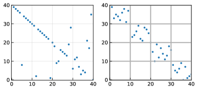
The work in [1] introduced the unlabeled sensing problem and establish that $n=2d$ measurements are necessary and sufficient for recovery of $\mathbf{x}^{*}$. Subsequent works [2, 3] have generalized this result and developed information theoretic inachievability analysis. Because estimating the unknown permutation matrix $\mathbf{P}^{*}$ is a challenging problem, several works [4, 5, 6, 7, 8, 9] assume a $k$-sparse, or partially shuffled, permutation model. [10, 11] consider an $r$-local, or block diagonal, permutation model. A permutation matrix $\mathbf{P}^{*}_{k}$ is $k$-sparse if it has $k$ off-diagonal elements, i.e., $\langle\mathbf{I},\mathbf{P}^{*}_{k}\rangle=n-k$. A permutation matrix $\mathbf{P}^{*}_{r}$ is $r$-local with $s$ blocks if $\mathbf{P}^{*}_{r}=\textrm{blkidag }(\mathbf{P}_{1},\cdots,\mathbf{P}_{s})$. Fig. 1 illustrates the two models. The two models are compared by information-theoretic inachiveability in [11].

For single-view unlabeled sensing, algorithms based on branch and bound and expectation maximization are proposed in [12, 13, 14]. These algorithms are applicable to small problem sizes. A stochastic alternating minimization approach is proposed in [15]. For multi-view unlabeled sensing, the Levsort subspace matching algorithm was proposed in [16]. A subspace clustering approach was proposed in [7]. The works [4, 5] propose methods based on bi-convex optimization and robust regression, respectively. A spectral initialization based method was proposed recently in [17].

1.1 Contributions

We extend our alternating minimization algorithm for the $r$-local unlabeled sensing model [10], [11] to the widely considered $k$-sparse model, Section II. We propose and analyze the initialization to our algorithm, Section III. Specifically, assuming random $\mathbf{B}$ or $\mathbf{X}^{*}$, we derive upper bounds on the initialization error for both $r$-local and $k$-sparse models. Numerical results and comparisons to baseline methods showing superior performance are given in Section IV.

A theoretical contribution is upper-bounding the error in the minimum norm solution to an under-determined linear inverse problem. Under-determined systems have also been studied as the sketching problem [18], but the results, derived assuming a random sub-sampling strategy and fixed $\mathbf{x}^{*}$, are not applicable as our sub-sampling strategy is deterministic because of the unknown permutation $\mathbf{P}^{*}$ in (1) and random $\mathbf{x}^{*}$.

1.2 Applications of unlabeled sensing

The linked linear regression problem [19, 20, 21], or linear regression under blocking, is to fit a linear model by minimizing over $\mathbf{x}$ and $\mathbf{P}$ the objective $\lVert\mathbf{y}-\mathbf{P}\mathbf{B}\mathbf{x}\rVert_{2}^{2}$, where $\mathbf{P}$ is an unknown $r$-local permutation. For example, consider a simple statistical model where the weight of an individual depends linearly on age and height. The vector $\mathbf{y}\in\mathbb{R}^{n}$ contains the weight of $n=10$ individuals, the matrix $\mathbf{B}\in\mathbb{R}^{n\times d}$, $d=2$ contains the values of the age, height of the individuals. The $10$ individuals comprise $5$ males, $5$ females and each record (weight, age, height) is known to belong to a male or a female individual. Letting the first (second) block of $5$ rows of $\mathbf{y},\mathbf{B}$ contain the records of male (female) individuals, the unknown $r$-local permutation, $r=5$, assigns each weight value (row of $\mathbf{y}$) to its corresponding age, height (row of $\mathbf{B})$. Experimental results and comparisons with baseline methods for the linked linear regression problem are given in Section 4.

For the pose and correspondence problem [22], the rows of $\mathbf{B}\in\mathbb{R}^{n\times d}$ contain the $d$-dimensional coordinates of the landmark points of an object. The object is transformed by an unknown linear transformation $\mathbf{X}^{*}$ and the rows of $\mathbf{Y}=\mathbf{P}^{*}\mathbf{B}\mathbf{X}^{*}$ contain the coordinates of the points of the transformed object. Given coordinates $\mathbf{B},\mathbf{Y}$, the problem is to assign a point in $\mathbf{B}$ to the corresponding point in $\mathbf{Y}$ and estimate the transformation $\mathbf{X}^{*}$. Another application of unlabeled sensing is signal amplitude estimation from binary quantized unlabeled samples [23]. The unknown scalar quantity $x$ is the signal amplitude and the sensing matrix $\mathbf{B}$ is replaced by a threshold function that models bit quantization. The image correspondence problem [24] and the $1$-d unassigned distance geometry problem (uDGP) were recently formulated as unlabeled sensing problems in [11].

Figure 1: Left. Sparse (or partially shuffled) permutation considered in [4, 5, 6, 7], with number of shuffles $k=10$. Right. The $r$-local permutation structure considered in [10], [11], with block size $r=10$. In this paper, we propose and analyze a general algorithm that is applicable to both permutation models.

1.3 Notation and definitions

$\mathbf{P}^{*}\in\Pi_{n}$ denotes a permutation matrix, where $\Pi_{n}=\{\mathbf{Z}\colon\mathbf{Z}\in\{0,1\}^{n\times n},\mathbf{Z}\mathbf{1}_{n}=\mathbf{1}_{n},\mathbf{Z}^{\intercal}\mathbf{1}_{n}=\mathbf{1}_{n}\}$ is the set of $n\times n$ permutation matrices and $\mathbf{1}_{n}\in\mathbb{R}^{n}$ is the vector of all ones. $\mathbf{P}^{*}_{r}$ denotes $r$-local permutations with block size $r$. $\mathbf{P}^{*}_{k}$ denotes $k$-sparse permutations with $k$ off-diagonal elements. The Hamming distortion $d_{H}=\Sigma_{i}\mathbbm{1}(\widehat{\mathbf{P}}(i)\neq\mathbf{P}(i))$ is the number of mismatches in permutation matrices $\widehat{\mathbf{P}},\mathbf{P}^{*}$. $\mathbf{A}^{\dagger}$ denotes the Moore-penrose pseudoinverse of matrix $\mathbf{A}$. $[\mathbf{A};\mathbf{B}]$ denotes the vertical concatenation of matrices $\mathbf{A}$ and $\mathbf{B}$. $\langle\mathbf{A},\mathbf{B}\rangle=\text{trace}(\mathbf{A}^{\intercal}\mathbf{B})$ denotes the matrix inner product. $\lVert\cdot\rVert_{p}$ denotes the vector $p$-norm and $\lVert\cdot\rVert_{F}$ denotes the matrix Frobenius norm. $\lVert X\rVert_{\varphi_{1}}(\lVert X\rVert_{\varphi_{2}})$ denotes the sub-exponential (sub-Gaussian) norm of the sub-exponential (sub-Gaussian) random variable $X$. $c^{\prime}\in\mathbb{R}$ denotes an absolute constant.

2 Algorithm

We propose to estimate the permutation $\mathbf{P}^{*}$ and the signal $\mathbf{X}^{*}$ by minimizing the forward error in $\eqref{eq:model}$,

$$(\widehat{\mathbf{P}},\widehat{\mathbf{X}})=\underset{\mathbf{P}\in\Pi_{n},\mathbf{X}}{\operatorname*{\mathrm{argmin}\,\,}}\,F(\mathbf{X},\mathbf{P})=\lVert\mathbf{Y}-\mathbf{P}\mathbf{B}\mathbf{X}\rVert_{F}^{2}.$$ (2)

Alternating minimization (alt-min) updates for (2) are

$$\mathbf{P}^{(t)}=\operatorname*{\mathrm{argmin}\,\,}_{\mathbf{P}\in\Pi_{n}}\langle-\mathbf{Y}{\mathbf{X}^{(t)}}^{\intercal}\mathbf{B}^{\intercal},\mathbf{P}\rangle,$$ (3)

$$\mathbf{X}^{(t+1)}=\operatorname*{\mathrm{argmin}\,\,}_{\mathbf{X}}F(\mathbf{X},\mathbf{P}^{(t)})={(\mathbf{P}^{(t)}\mathbf{B})}^{\dagger}\mathbf{Y}.$$ (4)

When the unknown permutation $\mathbf{P}^{*}$ is $r$-local, the $\mathbf{P}$ update in (3) decouples along the blocks of $\mathbf{P}^{*}$ and reduces to the simpler updates in line 9 of Algorithm 1. (2) is a non-convex optimization problem because the set of permutations is a discrete (non-convex) set. Therefore, the initialization to the updates (3), (4) has to be chosen carefully. We propose and analyze initializations for both $r$-local and $k$-sparse models in the following sections. A key contribution of our algorithm is that the model assumption is incorporated in the initialization. We note that Algorithm 1 for $r$-local $\mathbf{P}^{*}_{r}$ without initilization analysis was first proposed in our earlier work [11].

2.1 Initialization for the $r$-local model

When the unknown permutation $\mathbf{P}^{*}_{r}$ is $r$-local, we propose to initialize $\widehat{\mathbf{X}}$ by the collapsed initialization (7). Let $P_{i}$ denote each $r\times r$ block of $\mathbf{P}^{*}_{r}=\textrm{diag}(\mathbf{P}_{1},\cdots,\mathbf{P}_{s})$. Let $\mathbf{B}_{i}\in\mathbb{R}^{r\times d}$ denote blocks of the measurement matrix $\mathbf{B}=[\mathbf{B}_{1};\cdots;\mathbf{B}_{s}]$. Since the permutation $\mathbf{P}^{*}_{r}$ is block-diagonal, the $r$ permuted measurements in each block $[\mathbf{Y}_{i}:\mathbf{P}_{i}\mathbf{B}_{i}]$ are summed to extract one labelled measurement on $\mathbf{X}^{*}\in\mathbb{R}^{d\times m}$

$$\sum_{j=1}^{j=r}[\mathbf{P}_{i}\mathbf{B}_{i}(j)]^{\intercal}\mathbf{X}^{*}=\sum_{j=1}^{j=r}\mathbf{Y}_{i}(j)\enskip\forall i\in[s],$$ (5)

where $\mathbf{P}_{i}\mathbf{B}_{i}(j)\in{\mathbb{R}^{d\times 1}}$ denotes row $j$ of $\mathbf{P}_{i}\mathbf{B}_{i}$. Assuming all blocks have the same size $r$, the number of blocks is $s=n/r$. The $s$ labelled measurements in (5) are represented in the $s\times d$ collapsed linear system of equations

$$\widetilde{\mathbf{Y}}=\widetilde{\mathbf{B}}\mathbf{X}^{*},$$ (6)

where the rows of the collapsed measurement matrix $\widetilde{\mathbf{B}}\in\mathbb{R}^{s\times d}$ and measurements $\widetilde{\mathbf{Y}}\in\mathbb{R}^{s\times m}$ are

$$\widetilde{\mathbf{B}}(i)=\sum_{j=1}^{j=r}\mathbf{B}_{i}(j),\enskip\widetilde{\mathbf{Y}}(i)=\sum_{j=1}^{j=r}\mathbf{Y}_{i}(j)\enskip\hskip 3.00003pt\forall\hskip 1.00006pti\in[s].$$

Note that $\widetilde{\mathbf{B}}(i)=\sum_{j=1}^{j=r}\mathbf{P}_{i}\mathbf{B}_{i}(j)=\sum_{j=1}^{j=r}\mathbf{B}_{i}(j)$. The proposed initialization $\widehat{\mathbf{X}}$ is the minimum-norm solution to (6),

$$\widehat{\mathbf{X}}=\widetilde{\mathbf{B}}^{\dagger}\widetilde{\mathbf{Y}}.$$ (7)

Substituting the singular value decomposition form of $\widetilde{\mathbf{B}}^{\dagger}=\widetilde{\mathbf{V}}\mathbf{S}^{-1}\widetilde{\mathbf{U}}^{\intercal}$, where $\widetilde{\mathbf{B}}=\widetilde{\mathbf{U}}\mathbf{S}\widetilde{\mathbf{V}}^{\intercal}$, shows that $\widehat{\mathbf{X}}$ is the projection of $\mathbf{X}^{*}$ onto the the row space of $\widetilde{\mathbf{B}}$. Formally,

$$\lVert\mathbf{X}^{*}-\widehat{\mathbf{X}}\rVert_{2}=\lVert(\mathbf{I}-\widetilde{\mathbf{V}}\widetilde{\mathbf{V}}^{\intercal})\mathbf{X}^{*}\rVert_{2}.$$ (8)

For $s\geq d$, $\widehat{\mathbf{X}}=\mathbf{X}^{*}$. In section 3.1, we upper bound the error in initialization $\widehat{\mathbf{X}}$ for the under-determined $s<d$ case.

2.2 Initialization for the $k$-sparse model

When the unknown permutation $\mathbf{P}^{*}_{k}$ is $k$-sparse , we propose to initialize $\widehat{\mathbf{P}}^{(0)}=\mathbf{I}$, which sets $\widehat{\mathbf{Y}}^{(0)}=\mathbf{Y}=\mathbf{P}^{*}_{k}\mathbf{B}\mathbf{X}^{*}$. Since the permutation matrix $\mathbf{P}^{*}_{k}$ has $k$ off-diagonal elements, the initialization $\widehat{\mathbf{P}}^{(0)}=\mathbf{I}$ is close to the true solution $\mathbf{P}^{*}_{k}$ as $d_{H}(\widehat{\mathbf{P}}^{(0)},\mathbf{P}^{*}_{k})=k$. The initialization error is upper bounded in section 3.2.

Algorithm 1 alt-min

1:mode $\in\{r\text{-local},k\text{-sparse}\}$, convergence threshold $\epsilon$

2:if mode is $r$-local then

3:   $\widehat{\mathbf{X}}\leftarrow$ collapsed initialization in (7)

4:   $\widehat{\mathbf{Y}}\leftarrow\mathbf{B}\widehat{\mathbf{X}}$

5:else

6:   $\widehat{\mathbf{Y}}\leftarrow\mathbf{Y}$

7:while $\textrm{relative change}>\epsilon$ do

8:   if mode is $r$-local then

9:      for $i\in 1\cdots s$ do //$s$ is the number of blocks

10:         $\widehat{\mathbf{P}}_{i}\leftarrow{\operatorname*{\mathrm{argmin}\,\,}}_{\mathbf{P}_{i}\in\Pi_{r}}-\langle\mathbf{Y}_{i}\widehat{\mathbf{Y}}_{i}^{\intercal},\mathbf{P}_{i}\rangle$       

11:      $\widehat{\mathbf{\mathbf{P}}}\leftarrow\text{diag}(\widehat{\mathbf{P}}_{1},\cdots,\widehat{\mathbf{P}}_{s})$

12:   else  

13:      $\widehat{\mathbf{P}}={\operatorname*{\mathrm{argmin}\,\,}}_{\mathbf{P}\in\Pi_{n}}-\langle\mathbf{Y}\widehat{\mathbf{Y}}^{\intercal},\mathbf{P}\rangle$    

14:   $\widehat{\mathbf{X}}\leftarrow\mathbf{B}^{\dagger}\widehat{\mathbf{P}}^{\intercal}\mathbf{Y}$

15:   $\widehat{\mathbf{Y}}\leftarrow\mathbf{B}\widehat{\mathbf{X}}$

16:Return $\widehat{\mathbf{P}},\widehat{\mathbf{X}}$

3 Initialization analysis

3.1 $r$-local model

Assuming random models on either $\mathbf{B}$ or $\mathbf{X}^{*}$, the results in this section upper bound the error in the proposed initialization (7). Without any assumptions, the worst case error

$$\lVert\mathbf{x}^{*}-\hat{\mathbf{x}}\rVert_{2}^{2}\leq\frac{\lVert\mathbf{y}\rVert_{2}^{2}-\sigma^{2}_{\textrm{min}}(\mathbf{B})\lVert\hat{\mathbf{x}}\rVert_{2}^{2}}{\sigma^{2}_{\textrm{min}}(\mathbf{B})}$$ (9)

is achieved for $\mathbf{x}^{*}$ aligned with the direction of the singular vector corresponding to the smallest singular value $\sigma_{\textrm{min}}(\mathbf{B})$.

For $\mathbf{x}^{*}$ with zero-mean, independent sub-Gaussian random coordinates, Theorem $2.1$ in [25] shows that the error $\lVert\mathbf{x}^{*}-\hat{\mathbf{x}}\rVert_{2}$ is sub-Gaussian. In contrast, Theorem 1 in this work shows a sub-Gaussian error distribution for fixed $\mathbf{x}^{*}$ and Gaussian $\mathbf{B}$. Theorem 2 shows that the error is sub-Gaussian assuming fixed $\mathbf{B}$ and sub-Gaussian $\mathbf{x}^{*}$. Particularly, our result in Theorem 2 does not assume that the entries of $\mathbf{x}^{*}$ are independent.

Lemma 1.

Let $\hat{\mathbf{x}}$ be as defined in (7). Let $\mathbf{x}^{*}\in\mathbb{R}^{d}$ be the fixed unknown vector and let $\mathbf{B}$ be a Gaussian measurement matrix. For $t>0$,

$$\Pr_{\mathbf{B}}\Big{[}\frac{\lVert\mathbf{x}^{*}-\hat{\mathbf{x}}\rVert_{2}}{\lVert\mathbf{x}^{*}\rVert_{2}}\geq(1+t)\sqrt{\frac{d-s}{d}}\Big{]}\leq 2\exp(-c^{\prime}t^{2}(d-s)).$$ (10)

The result in (10) confirms that the relative error decreases with increasing number of measurements $s$ in the under-determined system. For example, let $s=3d/4$, the probability that the relative error exceeds $1/2$ decays with a sub-Gaussian tail. The bound in (10) is also sharp because it is the upper tail of the following two-sided inequality

$$\Pr_{\mathbf{B}}\Big{[}(1-t)\sqrt{\frac{d-s}{d}}\leq\frac{\lVert\mathbf{x}^{*}-\hat{\mathbf{x}}\rVert_{2}}{\lVert\mathbf{x}^{*}\rVert_{2}}\leq(1+t)\sqrt{\frac{d-s}{d}}\Big{]}\geq 1-2\exp(-c^{\prime}t^{2}(d-s)).$$

Proof of Lemma 1. Since $\mathbf{B}\in\mathbb{R}^{n\times d}$ is assumed Gaussian, the scaled collapsed matrix $\widetilde{\mathbf{B}}/\sqrt{`}r$ (6) is also a Gaussian matrix. The singular vectors of a rectangular Gaussian matrix $\mathbf{M}\in\mathbb{R}^{p\times q}$, $p>q$, span a $q$-dimensional uniformly random subspace of $\mathbb{R}^{p}$, see Section 5.2.6 in [26]. Therefore, $\hat{\mathbf{x}}=(\mathbf{I}-\widetilde{\mathbf{V}}\widetilde{\mathbf{V}}^{\intercal})\mathbf{x}^{*}$ is the projection of $\mathbf{x}^{*}\in\mathbb{R}^{d}$ onto a uniformly random $(d-s)$-dimensional subspace. The result in (10) follows from invoking the Johonson-Lindenstrauss (JL) Lemma (66) with $p=d$ and $q=d-s$.

Theorem 1.

Let $\widehat{\mathbf{X}}$ be as defined in (7). Let $\mathbf{X}^{*}\in\mathbb{R}^{d\times m}$ be the fixed unknown matrix and let $\mathbf{B}$ be a Gaussian measurement matrix. For $\log m\leq c^{\prime}t^{2}(d-s)/2$,

$$\Pr_{\mathbf{B}}\Big{[}\frac{\lVert\mathbf{X}^{*}-\widehat{\mathbf{X}}\rVert_{F}}{\lVert\mathbf{X}^{*}\rVert_{F}}\geq(1+t)\sqrt{\frac{d-s}{d}}\Big{]}\leq 2\exp(-c^{\prime}t^{2}(d-s)/2).$$ (11)

Proof of Theorem 1. Let event $\mathcal{E}=\bigcup_{i=1}^{i=m}\mathcal{E}_{i}$ be defined as the union of events $\mathcal{E}_{i}$, where

$$\mathcal{E}_{i}=\{\mathbf{x}^{*}\mid\lVert\mathbf{x}^{*}_{i}-\hat{\mathbf{x}}_{i}\rVert_{2}^{2}\geq\frac{(1+t)^{2}(d-s)}{d}\lVert\mathbf{x}^{*}_{i}\rVert_{2}^{2}\}.$$ (12)

Then,

$$\Pr\Big{[}\sum_{i=1}^{i=m}\lVert\mathbf{x}^{*}_{i}-\hat{\mathbf{x}}_{i}\rVert_{2}^{2}\leq\frac{(1+t)^{2}(d-s)}{d}\sum_{i=1}^{i=m}\lVert\mathbf{x}^{*}_{i}\rVert_{2}^{2}\Big{]}$$ (13)

$$\geq 1-\sum_{i=1}^{i=m}\Pr[\mathcal{E}_{i}]$$ (14)

$$\geq 1-2\exp(-c^{\prime}t^{2}(d-s)/2).$$ (15)

(14) follows from noting that $\Pr[\mathcal{E}^{c}]=1-\Pr[\mathcal{E}]$ and applying the union bound to $\mathcal{E}$. (15) is by substituting (10) and bounding $m\exp(-c^{\prime}t^{2}(d-s)/2)\leq 1$ for $\log m\leq c^{\prime}t^{2}(d-s)/2$.

Lemma 2.

Let $\hat{\mathbf{x}}$ be as defined in (7). Let $\mathbf{B}$ be a fixed measurement matrix and let $\mathbf{x}^{*}$ be a zero-mean sub-Gaussian random vector (31). For $t\geq 0$,

$$\Pr_{\mathbf{x}^{*}}\big{[}\lVert\mathbf{x}^{*}-\hat{\mathbf{x}}\rVert_{2}^{2}\geq c_{1}+2K^{2}(\sqrt{d-s}+1)t]\leq\exp(-t),$$ (16)

where $c_{1}=K^{2}(d-s+\frac{1}{2}\sqrt{d-s})$ and $K$ is as given in (31).

Proof of Lemma 2. The result in (16) follows from applying the Hanson-Wright inequality (65) to (8).

To derive the result in Theorem 2, it is necessary to show that $\lVert\mathbf{x}^{*}-\hat{\mathbf{x}}\rVert_{2}^{2}$ is a sub-exponential random variable. A random variable $X$ is sub-exponential if for $t\geq 0,K_{1}>0$

$$X\sim\textrm{subExp}\iff\Pr[\lvert X\rvert\geq t]\leq c^{\prime}\exp(-t/K_{1}),$$ (17)

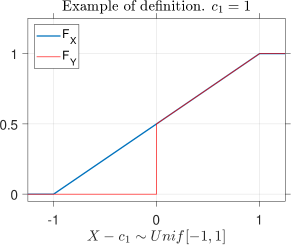
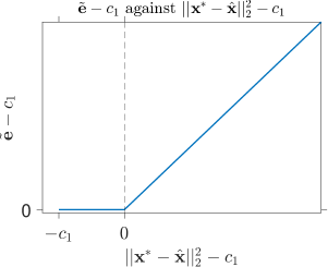
where $c^{\prime}\geq 1$. It cannot be concluded that the shifted random variable $\lVert\mathbf{x}^{*}-\hat{\mathbf{x}}\rVert_{2}^{2}-c_{1}$ is sub-exponential because the lower tail probability $\Pr[\lVert\mathbf{x}^{*}-\hat{\mathbf{x}}\rVert_{2}^{2}-c_{1}\leq-t],t>0$ is not upper bounded in (16). However, our goal is to upper bound the probability that the error exceeds a certain value. We therefore define the non-negative random variable $\tilde{\mathbf{e}}-c_{1}$, which upper bounds the lower tail as $\{\lVert\mathbf{x}^{*}-\hat{\mathbf{x}}\rVert_{2}^{2}-c_{1}\leq-t,t>0\}\leq 0$, see (18). The definition of $\tilde{\mathbf{e}}-c_{1}$ is given in (18), (19). Fig. 2 is a visual description of the definition. We show that $\tilde{\mathbf{e}}-c_{1}$ is a sub-exponential random variable in Lemma 3.

Figure 2: Left. The derived random variable (rv) $\tilde{\mathbf{e}}-c_{1}$ is plotted against the error rv $\lVert\mathbf{x}^{*}-\hat{\mathbf{x}}\rVert_{2}^{2}-c_{1}$. Note that i) $\tilde{\mathbf{e}}-c_{1}\geq 0$, ii) $\tilde{\mathbf{e}}-c_{1}\geq\lVert\mathbf{x}^{*}-\hat{\mathbf{x}}\rVert_{2}^{2}-c_{1}$, iii) $\tilde{\mathbf{e}}-c_{1}\mid\mathcal{E}_{1}=0$ and iv) $\tilde{\mathbf{e}}-c_{1}\mid\mathcal{E}_{2}=\lVert\mathbf{x}^{*}-\hat{\mathbf{x}}\rVert_{2}^{2}-c_{1}$. Right. Example. The cdfs of $Y(\tilde{\mathbf{e}}-c_{1})$ and $X(\lVert\mathbf{x}^{*}-\hat{\mathbf{x}}\rVert_{2}^{2}-c_{1})\sim\textrm{Unif}[-1,1]$ are plotted.

Lemma 3.

The random variable $\tilde{\mathbf{e}}-c_{1}$, defined in (18), (19), is a sub-exponential random variable with sub-exponential norm $\lVert\tilde{\mathbf{e}}-c_{1}\rVert_{\varphi_{1}}=c^{\prime}K_{1}$, where

$$\tilde{\mathbf{e}}-c_{1}\mid\mathcal{E}_{1}=0,$$ (18)

$$\tilde{\mathbf{e}}-c_{1}\mid\mathcal{E}_{2}=\lVert\mathbf{x}^{*}-\hat{\mathbf{x}}\rVert_{2}^{2}-c,$$ (19)

$c=K^{2}(d-s+\frac{1}{2}\sqrt{d-s})$, $K_{1}=2K^{2}(\sqrt{d-s}+1)$, $c^{\prime}$ is an absolute constant and events $\mathcal{E}_{1},\mathcal{E}_{2}$ are

$$\mathcal{E}_{1}=\{\mathbf{x}^{*}\mid\lVert\mathbf{x}^{*}-\hat{\mathbf{x}}\rVert_{2}^{2}-c_{1}\leq 0\},$$ (20)

$$\mathcal{E}_{2}=\mathcal{E}_{1}^{c}=\{\mathbf{x}^{*}\mid\lVert\mathbf{x}^{*}-\hat{\mathbf{x}}\rVert_{2}^{2}-c_{1}>0\}.$$ (21)

Proof of Lemma 3.

$$\Pr[\tilde{\mathbf{e}}-c_{1}\geq t] =\Pr[\tilde{\mathbf{e}}-c_{1}\geq t\mid\mathcal{E}_{1}]\cdot\Pr[\mathcal{E}_{1}]+\Pr[\tilde{\mathbf{e}}-c_{1}\geq t\mid\mathcal{E}_{2}]\cdot\Pr[\mathcal{E}_{2}]$$

$$=\Pr[\tilde{\mathbf{e}}-c_{1}\geq t\mid\mathcal{E}_{2}]\cdot\Pr[\mathcal{E}_{2}]$$ (22)

$$=\Pr[\lVert\mathbf{x}^{*}-\hat{\mathbf{x}}\rVert_{2}^{2}-c_{1}\geq t\mid\mathcal{E}_{2}]\cdot\Pr[\mathcal{E}_{2}]$$ (23)

$$=\Pr[\lVert\mathbf{x}^{*}-\hat{\mathbf{x}}\rVert_{2}^{2}-c_{1}\geq t],$$ (24)

where (22) follows from (18); specifically, $\Pr[\tilde{\mathbf{e}}-c_{1}\geq t\mid\mathcal{E}_{1}]=0\hskip 1.49994pt\forall\hskip 1.00006ptt>0$. (23) follows from (19) and (24) is by

$$\Pr[\lVert\mathbf{x}^{*}-\hat{\mathbf{x}}\rVert_{2}^{2}-c_{1}\geq t\mid\mathcal{E}_{2}]\Pr[\mathcal{E}_{2}]=\Pr[\lVert\mathbf{x}^{*}-\hat{\mathbf{x}}\rVert_{2}^{2}-c_{1}\geq t\cap\mathcal{E}_{2}]$$

and that the event $\{\mathbf{x}^{*}\mid\lVert\mathbf{x}^{*}-\hat{\mathbf{x}}\rVert_{2}^{2}-c_{1}\geq t,t>0\}$ is a subset of $\mathcal{E}_{2}$. From (16), for $t\geq 0$

$$\Pr\Big{[}\frac{\lVert\mathbf{x}^{*}-\hat{\mathbf{x}}\rVert_{2}^{2}-c_{1}}{2K^{2}(\sqrt{d-s}+1)}\geq t\Big{]}\leq\exp(-t).$$ (25)

From (24), for $t>0$

$$\Pr\Big{[}\frac{\lVert\mathbf{x}^{*}-\hat{\mathbf{x}}\rVert_{2}^{2}-c_{1}}{2K^{2}(\sqrt{d-s}+1)}\geq t\Big{]}=\Pr\Big{[}\frac{\tilde{\mathbf{e}}-c_{1}}{2K^{2}(\sqrt{d-s}+1)}\geq t\Big{]},$$ (26)

where $\sqrt{d-s}+1>0$ is a positive number since $s<d$, see (8). From (18) and (19), $\tilde{\mathbf{e}}-c_{1}$ is non-negative so that $\tilde{\mathbf{e}}-c_{1}=\lvert\tilde{\mathbf{e}}-c_{1}\rvert$ and

$$\Pr\Big{[}\frac{\tilde{\mathbf{e}}-c_{1}}{2K^{2}(\sqrt{d-s}+1)}\geq t\Big{]}=\Pr\Big{[}\frac{\lvert\tilde{\mathbf{e}}-c_{1}\rvert}{2K^{2}(\sqrt{d-s}+1)}\geq t\Big{]}.$$ (27)

Combining (26) and (27), for $t>0$

$$\Pr\Big{[}\frac{\lvert\tilde{\mathbf{e}}-c_{1}\rvert}{2K^{2}(\sqrt{d-s}+1)}\geq t\Big{]}=\Pr\Big{[}\frac{\lVert\mathbf{x}^{*}-\hat{\mathbf{x}}\rVert_{2}^{2}-c_{1}}{2K^{2}(\sqrt{d-s}+1)}\geq t\Big{]}.$$ (28)

Substituting (25) in (28), for $t>0$,

$$\Pr\Big{[}\frac{\lvert\tilde{\mathbf{e}}-c_{1}\rvert}{2K^{2}(\sqrt{d-s}+1)}\geq t\Big{]}\leq\exp(-t).$$ (29)

Since $\exp(0)=1$, (29) also holds at $t=0$

$$\Pr\Big{[}\frac{\lvert\tilde{\mathbf{e}}-c_{1}\rvert}{2K^{2}(\sqrt{d-s}+1)}\geq t\Big{]}\leq\exp(-t)\hskip 10.00002pt\forall\hskip 1.00006ptt\geq 0.$$ (30)

In (30), we have verified the definition in (17) for $\tilde{\mathbf{e}}-c_{1}$ with $K_{1}=2K^{2}(\sqrt{d-s}+1)$. By proposition 2.7.1 (a), (d) definition 2.7.5 in [26], and (30), the sub-exponential norm is $\lVert\tilde{\mathbf{e}}-c_{1}\rVert_{\varphi_{1}}=c^{\prime}K_{1}$.

Theorem 2.

Let $\mathbf{X}^{*}\in\mathbb{R}^{d\times m}$ be the unknown matrix such that the columns $\mathbf{x}^{*}_{i}$ are identical, independent, zero-mean sub-Gaussian random vectors, i.e., for $\alpha\in\mathbb{R}^{d}$, $K\geq 0$

$$\mathbb{E}[\exp(\alpha^{\intercal}\mathbf{x}_{i}^{*})]\leq\exp(\lVert\alpha\rVert_{2}^{2}K^{2}/2).$$ (31)

Let $\widehat{\mathbf{X}}$ be as defined in (7). Let $\mathbf{B}$ be a fixed measurement matrix. For $t\geq 0$,

$$\Pr\big{[}\sum_{i=1}^{i=m}\lVert\mathbf{x}^{*}_{i}-\hat{\mathbf{x}}_{i}\rVert_{2}-mc_{2}\geq t\big{]}\leq 2\exp\big{(}\frac{-c^{\prime}t^{2}}{mK_{1}}\big{)},$$ (32)

where $c_{2}=K(d-s+\frac{5}{2}\sqrt{d-s}+2)^{\frac{1}{2}}$, $K_{1}=2K^{2}(\sqrt{d-s}+1)$ and $c^{\prime}$ is an absolute constant.

Proof of Theorem 2. Note that

$$\Pr[\lvert\tilde{\mathbf{e}}-\mathbb{E}[\tilde{\mathbf{e}}]\rvert\geq t] =\Pr[\lvert\tilde{\mathbf{e}}-c_{1}-\mathbb{E}[\tilde{\mathbf{e}}-c_{1}]\rvert\geq t]$$

$$\leq 2\exp(-c^{\prime}t/\lVert\tilde{\mathbf{e}}-c_{1}-\mathbb{E}[\tilde{\mathbf{e}}-c_{1}]\rVert_{\varphi_{1}}).$$ (33)

Since $\lVert\tilde{\mathbf{e}}-c_{1}-\mathbb{E}[\tilde{\mathbf{e}}-c_{1}]\rVert_{\varphi_{1}}=c^{\prime}\lVert\tilde{\mathbf{e}}-c_{1}\rVert_{\varphi_{1}}$ (by 2.7.10 in [26]) and $\lVert\tilde{\mathbf{e}}-c_{1}\rVert_{\varphi_{1}}=c^{\prime}K_{1}$ (Lemma 3),

$$\Pr[\lvert\tilde{\mathbf{e}}-\mathbb{E}[\tilde{\mathbf{e}}]\rvert\geq t]\leq 2\exp(-c^{\prime}t/K_{1}),$$ (34)

where $K_{1}$ is as in (30). For $z\geq 0$, $\lvert z-1\rvert\geq\delta\implies\lvert z^{2}-1\rvert\geq\max(\delta,\delta^{2})$. Therefore,

$$\Pr\Big{[}\Big{\lvert}\frac{\sqrt{\tilde{\mathbf{e}}}-\sqrt{\mathbb{E}[\tilde{\mathbf{e}}]}}{\sqrt{\mathbb{E}[\tilde{\mathbf{e}}]}}\Big{\rvert}\geq\delta\Big{]} \leq\Pr\Big{[}\Big{\lvert}\frac{\tilde{\mathbf{e}}-\mathbb{E}[\tilde{\mathbf{e}}]}{\mathbb{E}[\tilde{\mathbf{e}}]}\Big{\rvert}\geq\max(\delta,\delta^{2})\Big{]}$$

$$\leq\Pr\Big{[}\Big{\lvert}\frac{\tilde{\mathbf{e}}-\mathbb{E}[\tilde{\mathbf{e}}]}{\mathbb{E}[\tilde{\mathbf{e}}]}\Big{\rvert}\geq\delta^{2}\Big{]}$$ (35)

$$\leq 2\exp(-c^{\prime}\mathbb{E}[\tilde{\mathbf{e}}]\delta^{2}/K_{1}),$$ (36)

where (36) follows by substituting $t=\delta^{2}$ in (34). Changing variables $t=\delta\sqrt{\mathbb{E}[\tilde{\mathbf{e}}]}$ in (36),

$$\Pr\big{[}\big{\lvert}\sqrt{\tilde{\mathbf{e}}}-\sqrt{\mathbb{E}[\tilde{\mathbf{e}}]}\big{\rvert}\geq t\big{]} \leq 2\exp(-c^{\prime}t^{2}/K_{1}).$$ (37)

From (37) and proposition 2.5.2 (i), (iv) and definition 2.5.6 in [26], the sub-Gaussian norm squared is bounded as

$$\lVert\sqrt{\tilde{\mathbf{e}}}-\sqrt{\mathbb{E}[\tilde{\mathbf{e}}]}\rVert_{\varphi_{2}}^{2}=c^{\prime}K_{1}.$$ (38)

Applying Hoeffding’s inequality (67) to $\sqrt{\tilde{\mathbf{e}}}-\sqrt{\mathbb{E}[\tilde{\mathbf{e}}]}$,

$$\Pr\big{[}\sum_{i=1}^{i=m}\big{(}\sqrt{\tilde{\mathbf{e}_{i}}}-\sqrt{\mathbb{E}[\tilde{\mathbf{e}}_{i}]}-\mathbb{E}[\sqrt{\tilde{\mathbf{e}}_{i}}-\sqrt{\mathbb{E}[\tilde{\mathbf{e}}_{i}]}]\big{)}\geq t\big{]}\leq 2\exp\big{(}\frac{-c^{\prime}t^{2}}{mK_{1}}\big{)}.$$ (39)

Substituting $\mathbb{E}[\sqrt{\tilde{\mathbf{e}}}]-\sqrt{\mathbb{E}[\tilde{\mathbf{e}}]}\leq 0$ (Jensen’s inequality) in (39),

$$\Pr\big{[}\sum_{i=1}^{i=m}\sqrt{\tilde{\mathbf{e}}_{i}}-m\sqrt{\mathbb{E}[\tilde{\mathbf{e}}]}\geq t\big{]}\leq 2\exp\big{(}\frac{-c^{\prime}t^{2}}{mK_{1}}\big{)}.$$ (40)

For non-negative random variable $X$, $\mathbb{E}[X]=\int_{0}^{\infty}\Pr[X>t]dt.$ Applied to ${\tilde{\mathbf{e}}-c_{1}}/{2K^{2}(\sqrt{d-s}+1)}$,

$$\mathbb{E}\Big{[}\frac{\tilde{\mathbf{e}}-c_{1}}{2K^{2}(\sqrt{d-s}+1)}\Big{]}\leq\int_{0}^{\infty}\exp(-t)dt=1$$ (41)

In (41), we have substituted the tail probability upper bounds from (30). Substituting $c_{1}$ from (16) in (41),

$$\mathbb{E}[\tilde{\mathbf{e}}]\leq K^{2}(d-s+\frac{5}{2}\sqrt{d-s}+2).$$ (42)

By definition in (18), (19) (also see Fig. 2), $\lVert\mathbf{x}^{*}_{i}-\hat{\mathbf{x}}_{i}\rVert_{2}\leq\sqrt{\tilde{\mathbf{e}}_{i}}\enskip\forall\enskip i\in[m]$. Substituting (42) and using $\lVert\mathbf{x}^{*}-\hat{\mathbf{x}}\rVert_{2}\leq\sqrt{\tilde{\mathbf{e}}}$ in (40) completes the proof.

Remark. Assuming Gaussian $\mathbf{B}$, Theorem $1$ shows that the probability that the relative error in (7) exceeds $\sqrt{(d-s)/d}$ decays at a sub-Gaussian rate. Assuming sub-Gaussian $\mathbf{x}^{*}$ instead, Theorem $2$ shows that the probability that the error exceeds $mc_{2}$, where $c_{2}$ as in (32), also decays at a sub-Gaussian rate. Both results agree that the estimate (7) improves as the number of measurements $s$ in the under-determined system (6) increases. The quantity $K$ in (32) depends linearly on the sub-Gaussian norm of $\mathbf{x}^{*}$ and can be estimated in practice. For $\mathbf{x}^{*}\sim\mathcal{N}(0,\mathbf{I})$, $K=1$. For $\mathbf{x}^{*}$ uniformly distributed on the Euclidean ball, $K=c^{\prime}$, where $c^{\prime}$ is an absolute constant.

3.2 $k$-sparse model

For the standard (un-permuted) linear inverse problem $\mathbf{y}=\mathbf{B}\mathbf{x}^{*}+\mathbf{w}$, the error in the solution $\lVert\mathbf{x}^{*}-\hat{\mathbf{x}}\rVert_{2}$ is upper bounded in terms of the noise $\lVert\mathbf{w}\rVert_{2}$ and $\sigma_{\min}(\mathbf{B})$, the smallest singular value of $\mathbf{B}$. In this section, we bound the error in the proposed initialization for the $k$-sparse permutation model in terms of the value of the objective function $F$, $\sigma_{\min}(\mathbf{B})$ and the number of shuffles $k$.

Lemma 4.

Let $\mathbf{P}^{*}_{k}$ be the fixed unknown $k$-sparse permutation matrix with $\langle\mathbf{I},\mathbf{P}^{*}_{k}\rangle=n-k$. Let $\mathbf{x}^{*}$ be the fixed unknown vector. Assuming Gaussian $\mathbf{B}$, let $\mathbf{y}^{*}=\mathbf{B}\mathbf{x}^{*}$, $\hat{\mathbf{y}}^{(0)}=\mathbf{P}^{*}_{k}\mathbf{B}\mathbf{x}^{*}$. For $k=1,\cdots,n-1$ and $t\geq 0$,

$$\Pr\big{[}\lVert\mathbf{y}^{*}-\hat{\mathbf{y}}^{(0)}\rVert_{2}^{2}\geq 2\lVert\mathbf{y}^{*}\rVert_{2}^{2}-2\lVert\mathbf{x}^{*}\rVert_{2}^{2}\big{(}n-k-c_{3}\sqrt{t}-3t\big{)}\big{]}\leq 7\exp(-t),$$ (43)

where $c_{3}=2\sqrt{n-k}+2\sqrt{3k}$.

Proof of Lemma 4. Under the $k$-sparse assumption on $\mathbf{P}^{*}$, the known vector $\mathbf{y}$ has $k$ shuffled entries. For $\widehat{\mathbf{P}}^{(0)}=\mathbf{I}$, i.e., $\hat{\mathbf{y}}^{(0)}=\mathbf{y}$, the forward error is

$$\lVert\mathbf{y}^{*}-\hat{\mathbf{y}}^{(0)}\rVert_{2}^{2}=2\lVert\mathbf{y}^{*}\rVert_{2}^{2}-2\langle\mathbf{y}^{*},\hat{\mathbf{y}}^{(0)}\rangle,$$ (44)

where $\mathbf{y}^{*}=\mathbf{B}\mathbf{x}^{*}$ is the unknown vector of unshuffled measurements. Since $\lVert\mathbf{y}^{*}\rVert_{2}=\lVert\hat{\mathbf{y}}^{(0)}\rVert_{2}$ and initialization $\hat{\mathbf{y}}^{(0)}=\mathbf{P}^{*}_{k}\mathbf{B}\mathbf{x}^{*}$ is known, the only unknown term in (44) is the inner product $\langle\mathbf{y}^{*},\hat{\mathbf{y}}^{(0)}\rangle$. The scaled inner product $\langle\mathbf{y}^{*},\hat{\mathbf{y}}^{(0)}\rangle/\lVert\mathbf{x}^{*}\rVert^{2}_{2}$ is expanded as

$$\frac{\langle\mathbf{y}^{*},\hat{\mathbf{y}}^{(0)}\rangle}{\lVert\mathbf{x}^{*}\rVert_{2}^{2}}=\frac{1}{\lVert\mathbf{x}^{*}\rVert_{2}^{2}}\sum_{i=1}^{i=n}\mathbf{b}_{i}^{\intercal}\mathbf{x}^{*}\mathbf{b}_{\mathbf{P}^{*}(i)}^{\intercal}\mathbf{x}^{*}$$ (45)

$$=\underbrace{\frac{1}{\lVert\mathbf{x}^{*}\rVert_{2}^{2}}\sum_{i=1}^{i=n-k}(\mathbf{b}_{i}^{\intercal}\mathbf{x}^{*})^{2}}_{\triangleq T_{1}}+\underbrace{\frac{1}{\lVert\mathbf{x}^{*}\rVert_{2}^{2}}\sum_{i=n-k+1}^{n}\mathbf{b}_{i}^{\intercal}\mathbf{x}^{*}\mathbf{b}_{\mathbf{P}^{*}(i)}^{\intercal}\mathbf{x}^{*}}_{\triangleq T_{2}}.$$

We have assumed in (45), wlog, that the last $k$ rows of $\mathbf{P}^{*}_{k}$ are shuffled. Assuming Gaussian $\mathbf{B}$, $(\mathbf{b}_{i}^{\intercal}\mathbf{x}^{*}/\lVert\mathbf{x}^{*}\rVert_{2})^{2}\sim\chi^{2}$ is Chi-squared distributed with $1$ degree of freedom. $T_{1}$, defined in (45), is the sum of $n-k$ independent Chi-square random variables and is bounded, using (69), as

$$\Pr\big{[}T_{1}\leq n-k-2\sqrt{(n-k)t}\big{]}\leq\exp(-t).$$ (46)

The product random variables in $T_{2}$ are distributed as the difference of two independent $\chi^{2}$ random variables. To see this, let

$$X={\mathbf{b}_{i}^{\intercal}\mathbf{x}^{*}}/{\lVert\mathbf{x}^{*}\rVert_{2}}\enskip,\enskip{Y=\mathbf{b}^{\intercal}_{\mathbf{P}(i)}\mathbf{x}^{*}}/{\lVert\mathbf{x}^{*}\rVert_{2}}.$$ (47)

The random variables $X$ and $Y$ in (47) are independent normal random variables. The product random variable $XY$ is expressed as

$$XY=\frac{1}{2}\big{(}\frac{X+Y}{\sqrt{2}}\big{)}^{2}-\frac{1}{2}\big{(}\frac{X-Y}{\sqrt{2}}\big{)}^{2}.$$ (48)

The random variables $(X+Y)/\sqrt{2}\sim\mathcal{N}(0,1)$ and $(X-Y)/\sqrt{2}\sim\mathcal{N}(0,1)$ are jointly Gaussian and uncorrelated. Therefore, $(X+Y)/\sqrt{2}$ is independent of $(X-Y)/\sqrt{2}$ and the product $XY$ is distributed as the difference of two independent $\chi^{2}$ distributed random variables $Z_{i}^{1},Z_{i}^{2}$

$$\frac{\mathbf{b}_{i}^{\intercal}\mathbf{x}^{*}\mathbf{b}_{\mathbf{P}(i)}^{\intercal}\mathbf{x}^{*}}{\lVert\mathbf{x}^{*}\rVert^{2}_{2}}\sim\frac{1}{2}Z^{1}_{i}-\frac{1}{2}Z^{2}_{i}\enskip\forall\enskip i\in n-k+1,\cdots,n.$$ (49)

The random variables (rv) in (49) are not mutually independent, but each rv depends on, at most, two other rvs. To see this, let permutation $\mathbf{P}$ such that $\mathbf{P}(i)\mapsto j$, then $\mathbf{b}_{i}^{\intercal}\mathbf{x}^{*}\mathbf{b}^{\intercal}_{j}\mathbf{x}^{*}$ is not independent of

$$\mathbf{b}^{\intercal}_{j}\mathbf{x}^{*}\mathbf{b}_{\mathbf{P}(j)}^{\intercal}\mathbf{x}^{*},\enskip\mathbf{b}^{\intercal}_{\mathbf{P}^{\intercal}(i)}\mathbf{x}^{*}\mathbf{b}^{\intercal}_{i}\mathbf{x}^{*}.$$ (50)

The $k$ rvs in (49) can therefore be partitioned into three sets $P,Q,R$ such that the rvs within each set are independent. Let $k_{1}$ be the number of rvs in set $P$. The sum $T_{P}$, where

$$T_{P}\triangleq\frac{1}{\lVert\mathbf{x}^{*}\rVert_{2}^{2}}\sum_{i\in P}\mathbf{b}_{i}^{\intercal}\mathbf{x}^{*}\mathbf{b}_{\mathbf{P}(i)}^{\intercal}\mathbf{x}^{*}=\frac{1}{2}\sum_{i\in P}Z^{1}_{i}-\frac{1}{2}\sum_{i\in P}Z^{2}_{i},$$ (51)

is upper bounded in probability as

$$\Pr[T_{P}\leq-2\sqrt{k_{1}t}-t]\leq 2\exp(-t).$$ (52)

(52) follows from applying the union bound to probabilities $p_{1},p_{2}$

$$p_{1} =\Pr\big{[}\sum_{i\in P}Z^{1}_{i}\leq k_{1}-2\sqrt{k_{1}t}\big{]}\leq\exp(-t),$$ (53)

$$p_{2} =\Pr\big{[}\sum_{i\in P}Z^{2}_{i}\geq k_{1}+2\sqrt{k_{1}t}+2t\big{]}\leq\exp(-t),$$ (54)

and bounding $p_{1},p_{2}$ using tail inequalities (69), (68), respectively. Defining $T_{Q},T_{R}$ similarly to (51), with cardinalities $k_{2}$, $k_{3}$ and applying the union bound as in (53), (54) gives

$$\Pr\big{[}T_{2}\leq-2(\sqrt{k_{1}t}+\sqrt{k_{2}t}+\sqrt{k_{3}t})-3t\big{]}\leq 6\exp(-t),$$ (55)

where $T_{2}=T_{P}+T_{Q}+T_{R}$. Since $\lVert[\sqrt{k_{1}}\enskip\sqrt{k_{2}}\enskip\sqrt{k_{3}}]^{\intercal}\rVert_{1}^{2}\leq 3\lVert\cdot\rVert_{2}^{2}=3k$, $\sqrt{k_{1}}+\sqrt{k_{2}}+\sqrt{k_{3}}\leq\sqrt{3k}$. Substituting in (55),

$$\Pr\big{[}T_{2}\leq-2\sqrt{3kt}-3t\big{]}\leq 6\exp(-t).$$ (56)

Applying the union bound to (46), (56) gives the result in (43).

Lemma 5.

For the same assumptions as in Lemma 4, $k=1,\cdots,n-1$ and $t\geq 0$,

$$\Pr\big{[}\sigma^{2}_{\min}(\mathbf{B})\lVert\mathbf{x}^{*}-\hat{\mathbf{x}}^{(1)}\rVert_{2}^{2}\geq 2\lVert\mathbf{y}^{*}\rVert_{2}^{2}-2\lVert\mathbf{x}^{*}\rVert_{2}^{2}\big{(}n-k-c_{3}\sqrt{t}-3t\big{)}\ -F^{(1)}\big{]}\leq 7\exp(-t),$$ (57)

where $\hat{\mathbf{x}}^{(1)}=\mathbf{B}^{\dagger}\hat{\mathbf{y}}^{(0)}$, $F^{(1)}=\lVert\mathbf{y}-\mathbf{B}\hat{\mathbf{x}}^{(1)}\rVert_{2}^{2}$ and $c_{3}=2\sqrt{n-k}+2\sqrt{3k}$.

Proof of Lemma 5. Let $\mathbf{e}$ denote the error term such that

$$\hat{\mathbf{y}}^{(0)}=\mathbf{B}\hat{\mathbf{x}}^{(1)}+\mathbf{e},$$ (58)

where $\hat{\mathbf{x}}^{(1)}=\mathbf{B}^{\dagger}\hat{\mathbf{y}}^{(0)}$, $\hat{\mathbf{y}}^{(0)}=\mathbf{P}^{*}_{k}\mathbf{B}\mathbf{x}^{*}$ and $\mathbf{e}\perp\mathcal{R}(\mathbf{B})$ is orthogonal to the range space of $\mathbf{B}$ because $\hat{\mathbf{x}}^{(1)}=\operatorname*{\mathrm{argmin}\,\,}_{\mathbf{x}}\lVert\hat{\mathbf{y}}^{(0)}-\mathbf{B}\mathbf{x}\rVert_{2}$. Substituting $\mathbf{y}^{*}=\mathbf{B}\mathbf{x}^{*}$ and (58) below,

$$\lVert\mathbf{y}^{*}-\hat{\mathbf{y}}^{(0)}\rVert_{2}^{2}=\lVert\mathbf{B}(\mathbf{x}^{*}-\hat{\mathbf{x}}^{(1)})-\mathbf{e}\rVert_{2}^{2}.$$ (59)

Using Pythogras’ theorem,

$$\lVert\mathbf{B}(\mathbf{x}^{*}-\hat{\mathbf{x}}^{(1)})-\mathbf{e}\rVert_{2}^{2}=\lVert\mathbf{B}(\mathbf{x}^{*}-\hat{\mathbf{x}}^{(1)})\rVert_{2}^{2}+\lVert\mathbf{e}\rVert_{2}^{2}.$$ (60)

Substituting the lower bound $\sigma^{2}_{\textrm{min}}(\mathbf{B})\lVert\mathbf{x}^{*}-\hat{\mathbf{x}}^{(1)}\rVert_{2}^{2}\leq\lVert\mathbf{B}(\mathbf{x}^{*}-\hat{\mathbf{x}}^{(1)})\rVert_{2}^{2}$ in (60),

$$\sigma^{2}_{\textrm{min}}(\mathbf{B})\lVert\mathbf{x}^{*}-\hat{\mathbf{x}}^{(1)}\rVert_{2}^{2}\leq\lVert\mathbf{y}^{*}-\hat{\mathbf{y}}^{(0)}\rVert_{2}^{2}-\lVert\mathbf{e}\rVert_{2}^{2}.$$ (61)

(62) follows by substituting the probability upper bound for $\lVert\mathbf{y}^{*}-\hat{\mathbf{y}}^{(0)}\rVert_{2}^{2}$ from (43) into (61) and noting that $\lVert\mathbf{e}\rVert_{2}^{2}=F^{(1)}=F(\widehat{\mathbf{P}}^{(0)},\hat{\mathbf{x}}^{(1)})$.

Theorem 3.

Let $\mathbf{P}^{*}_{k}$ be the fixed unknown permutation matrix with $\langle\mathbf{I},\mathbf{P}^{*}_{k}\rangle=n-k$. Let $\mathbf{X}^{*}$ be the fixed unknown matrix. Assuming Gaussian $\mathbf{B}$, let $\mathbf{Y}^{*}=\mathbf{B}\mathbf{X}^{*}$ and $\widehat{\mathbf{Y}}^{(0)}=\mathbf{P}^{*}_{k}\mathbf{B}\mathbf{X}^{*}$. For $k=1,\cdots,n-1$ and $t\geq\log m^{2}$,

$$\Pr\big{[}\sigma^{2}_{\min}(\mathbf{B})\lVert\mathbf{X}^{*}-\widehat{\mathbf{X}}^{(1)}\rVert_{F}^{2}\geq 2\lVert\mathbf{Y}^{*}\rVert_{F}^{2}-2\lVert\mathbf{X}^{*}\rVert_{F}^{2}\big{(}n-k-c_{3}\sqrt{t}-3t\big{)}-F^{(1)}\big{]}\leq 7\exp(-t),$$ (62)

where $\widehat{\mathbf{X}}^{(1)}=\mathbf{B}^{\dagger}\widehat{\mathbf{Y}}^{(0)}$, $F^{(1)}=\lVert\mathbf{Y}-\mathbf{B}\widehat{\mathbf{X}}^{(1)}\rVert_{F}^{2}$ and $c_{3}=2\sqrt{n-k}+2\sqrt{3k}$.

Proof of Theorem 3. The proof follows by applying the union bound to (57). An immediate upper bound that does not depend on the number of diagonal entries of $\mathbf{P}^{*}_{k}$ is

$$\sigma^{2}_{\textrm{min}}(\mathbf{B})\lVert\mathbf{X}^{*}-\widehat{\mathbf{X}}^{(1)}\rVert_{F}^{2}\leq 4\lVert\mathbf{Y}^{*}\rVert_{F}^{2}-F^{(1)}.$$ (63)

(62) shows that the probability that the error exceeds $\lVert\mathbf{Y}^{*}\rVert_{F}^{2}-c$, $c=\Omega(n-k)$ and $n-k$ is the number of diagonal entries in $\mathbf{P}^{*}_{k}$, decays exponentially. Furthermore, the term $\lVert\mathbf{Y}^{*}\rVert_{F}^{2}$ is known and $\lVert\mathbf{X}^{*}\rVert_{F}$ can be lower bounded in terms of known quantities as $\lVert\mathbf{X}^{*}\rVert^{2}_{F}\leq\lVert\mathbf{Y}^{*}\rVert^{2}_{F}/\sigma^{2}_{\max}(\mathbf{B})$.

4 Results

(a)

(b)

(c)

(d)

(e)

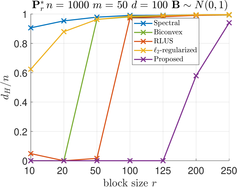
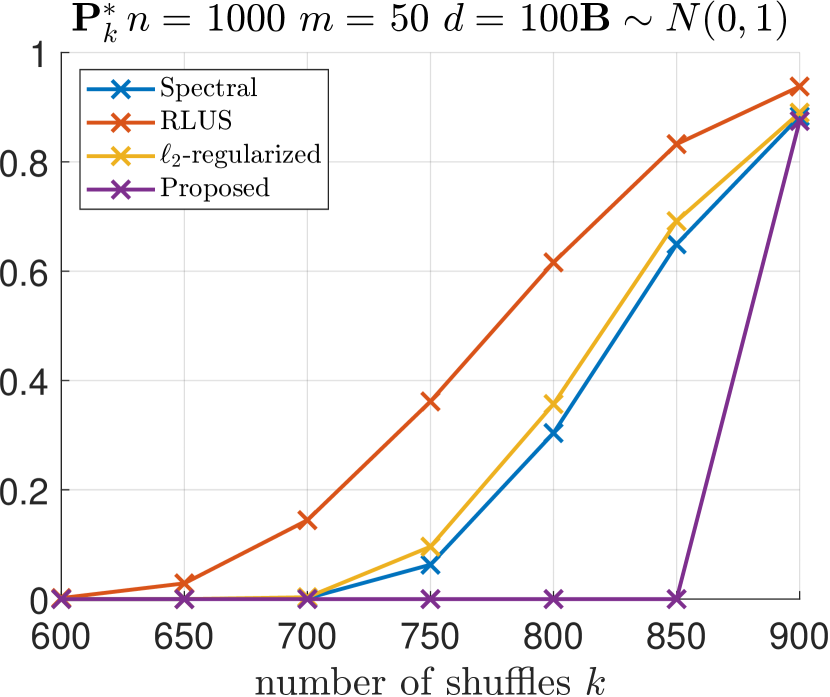
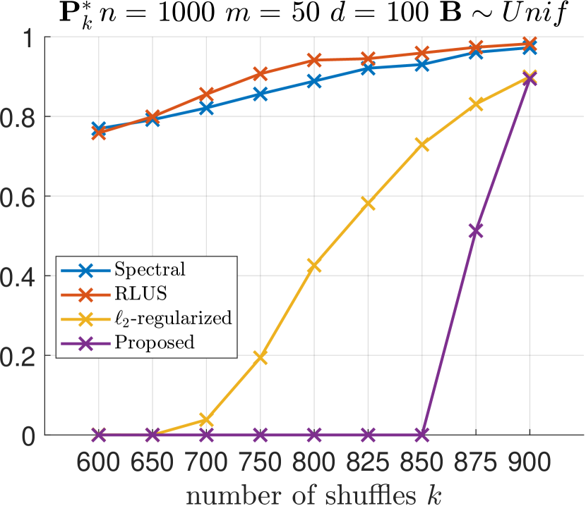
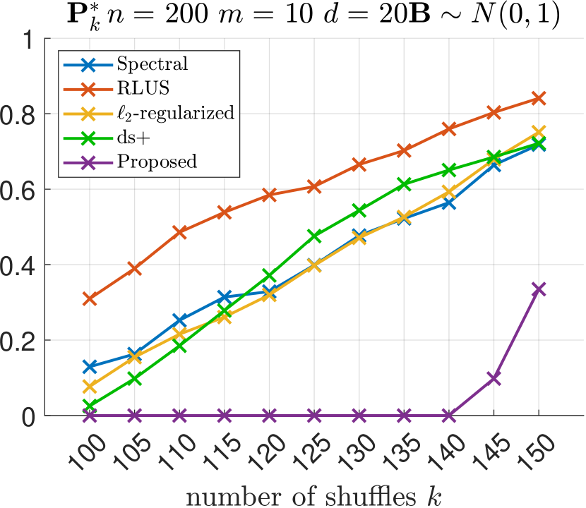
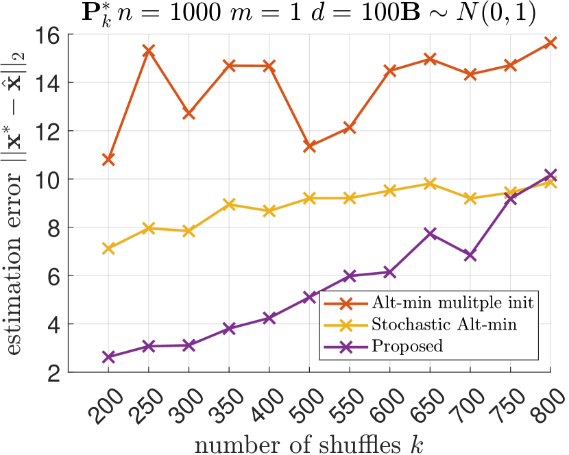
Figure 3: Synthetic simulations. $\mathbf{Y}=\mathbf{P}^{*}\mathbf{B}_{n\times d}\mathbf{X}^{*}_{d\times m}+\mathbf{W}$. The entries of $\mathbf{X}^{*}$ are drawn from the normal distribution. The permutation matrix $\mathbf{P}^{*}_{r}(\mathbf{P}^{*}_{k})$ is sampled uniformly from the set of $r$-local ($k$-sparse) permutations. The results are averaged over 15 Monte-Carlo runs. (a). Figure plots the fractional Hamming distortion $d_{H}/n$ against block size $r$. (b), (c), (d). Figure plots $d_{H}/n$ against number of shuffles $k$. (e). Figure plots the estimation error against $k$.

Dataset	$n$	$d$	$m$	$r_{\textrm{max}}$	$s$	Oracle	Naive	RLUS	$\ell_{2}$-reg	alt-min-$k$	alt-min-$r$
ftp	335	30	6	43	46	$(0.88,0)$	$(0.44,0.70)$	$(0.62,0.01)$	$(0.57,0.59)$	$(0.73,0.41)$	$(\mathbf{0.85},\mathbf{0.17})$
scm	8966	35	16	424	1137	$(0.58,0)$	$(0.21,0.79)$	$(0.52,0.29)$	$(0.46,0.49)$	$(0.54,0.22)$	$(\mathbf{0.55},\mathbf{0.22})$
scs	44484	10	6	3553	356	$(0.81,0)$	$(0.01,0.99)$	$(0.74,0.24)$	$(0.02,0.98)$	$(0.73,0.33)$	$(\mathbf{0.77},\mathbf{0.21})$
air-qty	27605	27	16	95	366	$(0.69,0)$	$(0.29,0.78)$	$(0.65,0.20)$	$(0.64,0.21)$	$\mathbf{(0.66,0.17)}$	$(0.65,0.19)$
air-qty	27605	27	16	46	744	$(0.69,0)$	$(0.10,0.94)$	$(0.60,0.34)$	$(0.26,0.79)$	$(0.57,0.42)$	$\mathbf{(0.62,0.32)}$

Table 1: $r_{\textrm{max}}$ denotes the largest block size of $\mathbf{P}^{*}_{r}$ and $s$ denotes the number of blocks. The methods are compared based on the coefficient of determination $R_{2}$ and relative error $(R_{2},\text{relative error})$. The relative error is $\lVert\mathbf{X}^{*}-\widehat{\mathbf{X}}\rVert_{F}/\lVert\mathbf{X}^{*}\rVert_{F}$, where $\mathbf{X}^{*}=\mathbf{B}^{\dagger}\mathbf{Y}^{*}$ is the ‘oracle’ regression matrix given unpermuted data $\mathbf{Y}^{*}$. The ‘naive’ estimate from permuted data $\mathbf{Y}$ is $\widehat{\mathbf{X}}=\mathbf{B}^{\dagger}\mathbf{Y}$. The coefficient $R_{2}(\widehat{\mathbf{X}})=1-(\lVert\mathbf{Y}^{*}-\mathbf{B}\widehat{\mathbf{X}}\rVert_{F}/\lVert\mathbf{Y}^{*}\rVert_{F})$ measures the goodness of fit for the unpermuted data.

MATLAB code and datasets are at the first author’s GitHub .

Baselines. We compare against six baseline methods. We refer to these methods as ‘$\ell_{2}$-regularized’ [5],‘ds+’ [5], ‘Spectral’ [17], ‘Biconvex’ [4], ‘RLUS’ [10], and ‘Stochastic alt-min’ [15]. The ‘$\ell_{2}$-regularized’ method considers the $k$-sparse permutation model and incorporates the model assumption by imposing a row-wise group sparse penalty on $\lVert\widehat{\mathbf{Y}}_{i,:}\rVert_{2}$, where $\widehat{\mathbf{Y}}=\mathbf{B}\widehat{\mathbf{X}}$. Other methods are discussed in the following paragraphs. We set $\epsilon=0.01$ in Algorithm 1.

Figs. 3(a), 3(b). We compare our algorithm for the $r$-local and $k$-sparse permutation models to baselines. To adapt the ‘Spectral’, ‘$\ell_{2}$-regularized’ and ‘Biconvex’ methods to the $r$-local model, we add a constraint enforcing the permutation estimates to be block-diagonal. The results show that our algorithm recovers $\mathbf{P}^{*}$ with decreasing block size $r$ and number of shuffles $k$. This observation confirms the conclusions of Theorems 1,2,3 as the initialization to our algorithm improves with lower values of $r$ and $k$. The results also show that our algorithm is applicable to both models, unlike baselines. Our algorithm is also computationally scalable. For $r=125$ in Fig. 3(a) and $k=850$ in Fig. 3(b), the MATLAB run-times, with 16 Gb RAM, are less than one second.

Fig. 3(c). The entries of the measurement matrix $\mathbf{B}$ are sampled i.i.d. from the uniform $[0,1]$ distribution. Compared to the case for Gaussian $\mathbf{B}$ (Fig. 3(b)), the performance of the ‘Spectral’ and ‘RLUS’ methods deteriorates significantly. This is because both algorithms consider quadratic measurements $\mathbf{Y}\mathbf{Y}^{\intercal}$. Specifically, the ‘Spectral’ method is based on the spectral initialization technique [27], which assumes that the measurement matrix is Gaussian. In contrast, the performance of the proposed algorithm and the ‘$\ell_{2}$-regularized’ method does not deteriorate.

Fig. 3(d). The ‘ds+’ algorithm [5] considers the convex relaxation of (2) by minimizing the objective over the set of doubly stochastic matrices. Assuming an upper bound on the number of shuffles $k$ is known, ‘ds+’ also constrains $\langle\mathbf{I},\mathbf{P}\rangle\geq n-k$. Each iteration of ‘ds+’ minimizes a linear program, greatly increasing the run-time of the algorithm. The results show that the proposed algorithm outperforms ‘ds+’, possibly because, for our algorithm, the objective is optimized directly over the set of permutations.

Fig. 3(e). We compare to the method in [15] which considers the $m=1$ single-view setup and proposes stochastic alternating minimization (S.alt-min) to optimize (2). The run-time for S.alt-min is 50 times the run-time of the proposed algorithm because S.alt-min updates $\mathbf{P}$ multiple times in each iteration and retains the best update. [15] also proposes alt-min with multiple initializations for $\widehat{\mathbf{P}}^{(0)}$. The results in Fig. 3(e) show that our algorithm (alt-min with $\widehat{\mathbf{P}}^{(0)}=\mathbf{I}$ initialization) outperforms both S.alt-min and alt-min with multiple initializations.

Real data. For the linked linear regression problem introduced in Section 1.2, we report results in Table 1 on the four datasets from [5]. The measurement matrix and the regression model are also defined as in [5]. For ‘ftp’,‘scm’ and ‘scs’, the values of a feature (or column of the measurement matrix) are rounded and data points with the same feature value are assigned to the same block and permuted. The ‘air-qty’ dataset comprises time-stamped readings with year, month, day and hour information. In row 4 (5) of Table 1, readings with the same month and day (day and hour) are assigned to the same block and permuted, as also done in [5]. The results show that the proposed alt-min algorithm outperforms the competing baselines. ‘alt-min-$k$’, i.e. alt-min initialized to $\widehat{\mathbf{P}}^{(0)}=\mathbf{I}$, is also competitive, possibly because permuting correlated rows may not greatly corrupt the measurement matrix $\mathbf{B}$.

5 Conclusion

We propose and analyze the alternating minimization algorithm with a model-dependent initialization for the unlabeled sensing problem. The analysis is insightful and explains the superior performance of the algorithm compared to baseline methods. As part of future work, we plan to i) characterize the rate of convergence, ii) analyze the second-order convergence properties of the proposed algorithm, and iii) explore if our analysis also holds for other random signal models by considering concentration inequality results such as [28].

Acknowledgment: Abiy Tasissa would like to thank Professor Radosław Adamczak for correspondence on his work in [28].

6 Appendix

Hanson Wright Inequality.

From Theorem 2.1 in [29], let $\mathbf{\Sigma}=\mathbf{A}^{\intercal}\mathbf{A}$ be a positive semi-definite matrix. Let $\mathbf{x}=(x_{1},\cdots,x_{d})$ be a zero-mean sub-Gaussian random vector. i.e., for $\alpha\in\mathbb{R}^{d}$, $K\geq 0$

$$\mathbb{E}[\exp(\alpha^{\intercal}\mathbf{x}^{*})]\leq\exp(\lVert\alpha\rVert_{2}^{2}K^{2}/2).$$ (64)

For $t\geq 0$,

$$\Pr[\lVert\mathbf{A}\mathbf{x}\rVert_{2}^{2}\geq K^{2}(tr(\mathbf{\Sigma})+2\sqrt{tr(\mathbf{\Sigma}^{2})t}+2t\lVert\mathbf{\Sigma}\rVert)]\leq\exp(-t).$$ (65)

To derive the result in (16), set $\mathbf{A}=(\mathbf{I}-\widetilde{\mathbf{V}}\widetilde{\mathbf{V}}^{\intercal})$, as in (8). Since $\mathbf{A}\in\mathbb{R}^{d\times d}$ is a $(d-s)$-dimensional projection matrix, the matrix $\mathbf{\Sigma}=\mathbf{A}^{\intercal}\mathbf{A}=\mathbf{A}\mathbf{A}=\mathbf{A}$ is also a projection matrix. Therefore, $tr(\mathbf{\Sigma})=tr(\mathbf{\Sigma}^{2})=tr(\mathbf{A})=d-s$ and $\lVert\mathbf{\Sigma}\rVert=1$. Next, upper bound $2\sqrt{tr(\mathbf{\Sigma}^{2})t}\leq 2t\sqrt{tr(\mathbf{\Sigma}^{2})}+\frac{1}{2}\sqrt{tr(\mathbf{\Sigma}^{2})}$.

Johnson Lindenstrauss Lemma.

Let $P$ be a projection in $\mathbb{R}^{p}$ onto a uniformly distributed random $q$-dimensional subspace. Let $z\in\mathbb{R}^{p}$ be a fixed point and $t>0$. Then, with probability at least $1-2\exp(-ct^{2}q)$,

$$(1-t)\sqrt{\frac{q}{p}}\lVert z\rVert_{2}\leq\lVert Pz\rVert_{2}\leq(1+t)\sqrt{\frac{q}{p}}\lVert z\rVert_{2}.$$ (66)

Hoeffdings’ inequality. Theorem 2.6.2 in [26].

Let $X_{1},\cdots,X_{m}$ be independent, sub-Gaussian random variables. Then, for every $t\geq 0$,

$$\Pr\big{[}\lvert\sum_{i=1}^{i=m}X_{i}-\mathbb{E}[X_{i}]\rvert\geq t\big{]}\leq 2\exp\Big{(}\frac{-c^{\prime}t^{2}}{\sum_{i=1}^{i=m}\lVert X_{i}\rVert_{\varphi_{2}}^{2}}\Big{)},$$ (67)

where $\lVert X_{i}\rVert_{\varphi_{2}}$ denotes the sub-Gaussian norm of $X_{i}$ and $c^{\prime}$ is an absolute constant.

Tail inequality for $\chi^{2}_{D}$ distributed random variables [30].

Let $Z_{D}$ be a $\chi^{2}$ statistic with $D$ degrees of freedom. For any positive $t$,

$$\Pr[Z_{D}\geq D+2\sqrt{Dt}+2t] \leq\exp(-t),$$ (68)

$$\Pr[Z_{D}\leq D-2\sqrt{Dt}] \leq\exp(-t).$$ (69)

References

• [1] Jayakrishnan Unnikrishnan, Saeid Haghighatshoar, and Martin Vetterli. Unlabeled sensing with random linear measurements. IEEE Trans. Inf. Theory, 64(5):3237โ€“3253, 2018.
• [2] I.ย Dokmaniฤ‡. Permutations unlabeled beyond sampling unknown. IEEE Signal Processing Letters, 26(6):823โ€“827, 2019.
• [3] A.ย Pananjady, M.ย J. Wainwright, and T.ย A. Courtade. Linear regression with shuffled data: Statistical and computational limits of permutation recovery. IEEE Trans. Inf. Theory, 64(5):3286โ€“3300, 2018.
• [4] Hang Zhang, Martin Slawski, and Ping Li. Permutation recovery from multiple measurement vectors in unlabeled sensing. In 2019 IEEE Int. Symposium on Inf. Theory (ISIT), pages 1857โ€“1861, 2019.
• [5] Martin Slawski, Emanuel Ben-David, and Ping Li. Two-stage approach to multivariate linear regression with sparsely mismatched data. J. Mach. Learn. Res., 21(204):1โ€“42, 2020.
• [6] Hang Zhang and Ping Li. Optimal estimator for unlabeled linear regression. In Proceedings of the 37th Int. Conference on Machine Learning (ICML), 2020.
• [7] Martin Slawski, Mostafa Rahmani, and Ping Li. A sparse representation-based approach to linear regression with partially shuffled labels. In Uncertainty in Artificial Intelligence, pages 38โ€“48. PMLR, 2020.
• [8] Xuย Shi, Xiaoou Li, and Tianxi Cai. Spherical regression under mismatch corruption with application to automated knowledge translation. Journal of the American Statistical Association, 116(536):1953โ€“1964, 2021.
• [9] Martin Slawski and Emanuel Ben-David. Linear regression with sparsely permuted data. Electronic Journal of Statistics, 13(1):1โ€“36, 2019.
• [10] Ahmedย Ali Abbasi, Abiy Tasissa, and Shuchin Aeron. R-local unlabeled sensing: A novel graph matching approach for multiview unlabeled sensing under local permutations. IEEE Open Journal of Signal Process., 2:309โ€“317, 2021.
• [11] Ahmedย Ali Abbasi, Abiy Tasissa, and Shuchin Aeron. r-local unlabeled sensing: Improved algorithm and applications. In ICASSP 2022 - 2022 IEEE International Conference on Acoustics, Speech and Signal Processing (ICASSP), pages 5593โ€“5597, 2022.
• [12] V.ย Emiya, A.ย Bonnefoy, L.ย Daudet, and R.ย Gribonval. Compressed sensing with unknown sensor permutation. In 2014 IEEE Int. Conference on Acoustics, Speech and Signal Processing (ICASSP), pages 1040โ€“1044, 2014.
• [13] Liangzu Peng and Manolisย C. Tsakiris. Linear regression without correspondences via concave minimization. IEEE Signal Proces. Letters, 27:1580โ€“1584, 2020.
• [14] Liangzu Peng, Xuming Song, Manolisย C Tsakiris, Hayoung Choi, Laurent Kneip, and Yuamming Shi. Algebraically-initialized expectation maximization for header-free communication. In IEEE Int. Conf. on Acous., Speech and Signal Process. (ICASSP), pages 5182โ€“5186. IEEE, 2019.
• [15] Abubakar Abid and James Zou. A stochastic expectation-maximization approach to shuffled linear regression. In 2018 56th Annual Allerton Conference on Communication, Control, and Computing (Allerton), pages 470โ€“477. IEEE, 2018.
• [16] A.ย Pananjady, M.ย J. Wainwright, and T.ย A. Courtade. Denoising linear models with permuted data. In 2017 IEEE Int. Symposium on Inf. Theory (ISIT), pages 446โ€“450, 2017.
• [17] Hang Zhang and Ping Li. Optimal estimator for unlabeled linear regression. In Int. Conference on Machine Learning, pages 11153โ€“11162. PMLR, 2020.
• [18] Davidย P Woodruff etย al. Sketching as a tool for numerical linear algebra. Foundations and Trendsยฎ in Theoretical Computer Science, 10(1โ€“2):1โ€“157, 2014.
• [19] Jaredย S Murray. Probabilistic record linkage and deduplication after indexing, blocking, and filtering. Journal of Privacy and Confidentiality 7 (1)., 2016.
• [20] Partha Lahiri and Michaelย D Larsen. Regression analysis with linked data. Journal of the American statistical association, 100(469):222โ€“230, 2005.
• [21] Ying Han and Partha Lahiri. Statistical analysis with linked data. International Statistical Review, 87:S139โ€“S157, 2019.
• [22] Manuel Marques, Marko Stoลกiฤ‡, and Joฤo Costeira. Subspace matching: Unique solution to point matching with geometric constraints. In 2009 IEEE 12th Int. Conference on Computer Vision, pages 1288โ€“1294, 2009.
• [23] Guanyu Wang, Jiang Zhu, Rickย S. Blum, Peter Willett, Stefano Marano, Vincenzo Matta, and Paolo Braca. Signal amplitude estimation and detection from unlabeled binary quantized samples. IEEE Transactions on Signal Processing, 66(16):4291โ€“4303, 2018.
• [24] Gonzalo Mena, David Belanger, Scott Linderman, and Jasper Snoek. Learning latent permutations with gumbel-sinkhorn networks, 2018.
• [25] Mark Rudelson and Roman Vershynin. Hanson-Wright inequality and sub-gaussian concentration. Electronic Communications in Probability, 18(none):1 โ€“ 9, 2013.
• [26] Roman Vershynin. High-dimensional probability: An introduction with applications in data science, volumeย 47. Cambridge university press, 2018.
• [27] Wangyu Luo, Wael Alghamdi, and Yueย M. Lu. Optimal spectral initialization for signal recovery with applications to phase retrieval. IEEE Transactions on Signal Processing, 67(9):2347โ€“2356, 2019.
• [28] Radoslaw Adamczak. A note on the hanson-wright inequality for random vectors with dependencies. Electronic Communications in Probability, 20:1โ€“13, 2015.
• [29] Daniel Hsu, Sham Kakade, and Tong Zhang. A tail inequality for quadratic forms of subgaussian random vectors. Electronic Communications in Probability, 17:1โ€“6, 2012.
• [30] B.ย Laurent and P.ย Massart. Adaptive estimation of a quadratic functional by model selection. The Annals of Statistics, 28(5):1302 โ€“ 1338, 2000.