Stability estimates for the expected utility in Bayesian optimal experimental design

Duc-Lam Duonglabel=e1]duc-lam.duong@lut.fi [    Tapio Helinlabel=e2]tapio.helin@lut.fi [    Jose Rodrigo Rojo-Garcialabel=e3]rodrigo.rojo.garcia@lut.fi [ Computational Engineering, LUT School of Engineering Science, Lappeenranta-Lahti University of Technology, Finlandpresep=, ]e1,e2,e3
Abstract

We study stability properties of the expected utility function in Bayesian optimal experimental design. We provide a framework for this problem in a non-parametric setting and prove a convergence rate of the expected utility with respect to a likelihood perturbation. This rate is uniform over the design space and its sharpness in the general setting is demonstrated by proving a lower bound in a special case. To make the problem more concrete we proceed by considering non-linear Bayesian inverse problems with Gaussian likelihood and prove that the assumptions set out for the general case are satisfied and regain the stability of the expected utility with respect to perturbations to the observation map. Theoretical convergence rates are demonstrated numerically in three different examples.

Bayesian optimal experimental design,
inverse problems,
stability,
keywords:
\startlocaldefs\endlocaldefs
thanks: Address for correspondence: Department of Computational Engineering, School of Engineering Science, LUT University, Yliopistonkatu 34, 53850 Lappeenranta, Finland.

, and

1 Introduction

Acquisition of high quality data is the crux of many challenges in science and engineering. An outstanding example is the parameter estimation problem in statistical models. Namely, data collection, whether in field experiments or in laboratory, is often restricted by limited resources. It can be difficult, expensive and time-consuming, which puts severe limits on the quality of data acquired. To maximize the value of data for inference and minimize the uncertainty of the estimated parameters, one has to design the experiment (for instance, placing the sensors) in a way that is as economical and efficient as possible. This involves choosing the values of the controllable variables before the experiment takes place. Carefully designed experiments can make a substantial difference in accomplishing the tasks in an appropriate manner. Optimal experimental design (OED) is a mathematical framework where a set of design variables with certain optimal criteria (based on the information matrix derived from the model) are satisfied (Steinberg and Hunter (1984); Pukelsheim (2006)). The most common criteria for OED include A-optimality and D-optimality which, in finite dimensions, seeks to minimize the trace and the determinant of the Fisher information matrix, respectively.

We adopt a Bayesian approach to OED (Chaloner and Verdinelli, 1995) that formulates the task as a maximization of an expected utility. Suppose X𝑋X denotes our unknown parameter, Y𝑌Y stands for the observation and d𝑑d the design parameter. The expected utility U𝑈U is given by

U(d)=𝔼μu(X,Y;d),𝑈𝑑superscript𝔼𝜇𝑢𝑋𝑌𝑑U(d)=\mathbb{E}^{\mu}u(X,Y;d), (1)

where u(X,Y;d)𝑢𝑋𝑌𝑑u(X,Y;d) denotes the utility of an estimate X𝑋X given observation Y𝑌Y with design d𝑑d, and the expectation is taken w.r.t. the joint distribution μ𝜇\mu of X𝑋X and Y𝑌Y. The task of optimizing U(d)𝑈𝑑U(d) is notoriously expensive especially if the design space is large or X𝑋X and Y𝑌Y are modelled in high-dimensional space (Ryan et al., 2016).

The guiding set of design problems for this paper is those emerging in modern inverse problems (Engl, Hanke and Neubauer, 1996), which often involve imaging a high-dimensional object by indirect observations. Bayesian approach to inverse problems has gained considerable interest during the last two decades (Kaipio and Somersalo (2006); Stuart (2010); Dashti and Stuart (2017)). The underlying mathematical model in inverse problems is often governed by partial differential equations (PDEs) giving rise to complex high-dimensional likelihood models.

Exploring the complex high-dimensional posterior distributions in Bayesian inversion is computationally costly but has become standard in literature in recent years due to developments in Monte Carlo (MC) based sampling schemes and the growth of available computational resources. To accelerate this task, various approximation schemes such as surrogate modelling of the likelihood distribution can also be applied including e.g. polynomial chaos expansion (Marzouk, Najm and Rahn, 2007; Schillings and Schwab, 2013) or neural networks (Herrmann, Schwab and Zech, 2020). Moreover, stability of the posterior distribution with respect to such approximations is well-understood (see Sprungk (2020); Garbuno-Inigo et al. (2023) and reference therein).

In the OED framework, the computational effort compared to conventional Bayesian inversion is significantly larger due to the double expectation and optimization task. In consequence, approximation schemes have a key role in producing optimal designs in that framework. However, questions about the stability of the expected utility have received limited attention. To the best of our knowledge, it has been only considered in terms of a fixed design, i.e., pointwise convergence of the expected utility. Tempone and others in (Beck et al., 2018, 2020; Long et al., 2015) have developed approximation results for nested MC methods with and without utilising an additional Laplace approximation and analyse the optimal parametrisation of the method with respect to the approximation error versus computational effort. Since MC approximation is random, any such error bound is expressed in probabilistic terms. In particular, Beck et al. (2018) provides a recipe to achieve a given probabilistic error tolerance with optimal computational effort. In another recent line of work, Foster and others (Foster et al., 2019) develop error analysis for variational methods being applied in combination with MC methods and optimize the depth of variational approximation to achieve a rate of convergence 𝒪((N+K)12)𝒪superscript𝑁𝐾12{\mathcal{O}}((N+K)^{-\frac{1}{2}}) for N𝑁N samples from MC and K𝐾K optimization steps for the variational model.

For Bayesian OED tasks involving optimization on a continuous design manifold (as is often the case in inverse problems), pointwise convergence does not provide the full picture of the stability in terms of the optimization task. Instead, uniform approximation rates of given numerical schemes in a neighbourhood around the optimal design are preferable in that regard. In this work, we study the uniform stability of the expected utility in Bayesian OED systematically where changes in likelihood function or observation map can be observed.

Non-parametric inference in Bayesian inverse problems and OED is motivated by the conviction to leave discretization until the last possible moment (Stuart, 2010), hence giving rise to opportunities to choose appropriate and robust discretization methods. Non-parametric approach for OED in Bayesian inverse problems has been formalized by Alexanderian (see Alexanderian (2021) and references therein). Let us note that the infinite-dimensional setting arises naturally in numerous works involving Bayesian OED in inverse problems constrained by PDEs (Alexanderian et al. (2014); Long, Motamed and Tempone (2015); Alexanderian et al. (2016); Alexanderian, Gloor and Ghattas (2016); Beck et al. (2018); Wu, Chen and Ghattas (2020), to name a few), integral geometry (Haber, Horesh and Tenorio, 2008; Ruthotto, Chung and Chung, 2018; Burger et al., 2021; Helin, Hyvönen and Puska, 2022) or nonlinear systems (Huan and Marzouk, 2013, 2014).

1.1 Our contribution

This work contributes to the rigorous study of the mathematical framework of Bayesian OED.

  • We formulate the OED stability problem under a Bayesian framework in a non-parametric setting. We propose a set of assumptions (along the lines of Stuart (2010)) under which the stability problem for OED can be addressed in a systematic way (Assumption 3.1). In particular, we assume that the likelihood and its approximate version are close in the Kullback–Leibler divergence.

  • We establish the convergence of the expected utility for a general approximation scheme satisfying Assumption 3.1 with a rate of one-half of the likelihood convergence rate (see Theorem 3.4). We demonstrate by a trivial example that a faster rate is not possible without further assumptions (see Example 1).

  • Together with the convergence of the surrogate expected utility, we prove that their maximizers converge, up to a subsequence, to a maximizer of the true expected utility (see Theorem 3.5). This ensures that the optimal design variable is also stable in the approximation.

  • As an important application, we consider some Bayesian inverse problems with Gaussian noise and their observation map can be replaced by some surrogate model. We demonstrate that the assumptions we set out previously are satisfied in this case, given that the observation map and its surrogate model are close in certain norms (see Proposition 4.2 and Theorem 4.4).

  • Finally, we carry out numerical simulations on three different design problems. We observe that the rates predicted by our main theorems are aligned with the numerical results.

1.2 Structure of the paper

The paper is organised as follows. In Section 2, we give an overview of the main objects of this article, including basic notions of non-parametric Bayesian inverse problems and Bayesian experimental design. We also summarize some background in probability measure theory, commonly used metrics between measures and introduce notations that will be used throughout this paper. In Section 3, we first outline the common framework including the general assumptions and main results. We proceed by establishing several lemmas and proving our main theorems. An important aspect of the main results is considered in Section 4 where we study the stability of OED for some Bayesian inverse problems with Gaussian noise. In the last section, we provide three numerical examples to illustrate the results of the paper.

2 Preliminaries

2.1 Probability measures and metrics between measures

Throughout this paper, 𝒳𝒳\mathcal{X} will be a separable Banach space (Hilbert space) equipped with a norm 𝒳\left\|\cdot\right\|_{\mathcal{X}} (inner product ,𝒳subscript𝒳\langle\cdot\,,\,\cdot\rangle_{\mathcal{X}}), with notice that the subscript may be ignored if no confusion arises. A bounded linear operator 𝒞:𝒳𝒳:𝒞𝒳𝒳\mathcal{C}:\mathcal{X}\to\mathcal{X} in Hilbert space 𝒳𝒳\mathcal{X} is called self-adjoint if 𝒞x,y=x,𝒞y𝒞𝑥𝑦𝑥𝒞𝑦\langle\mathcal{C}x,y\rangle=\langle x,\mathcal{C}y\rangle for all x,y𝒳𝑥𝑦𝒳x,y\in\mathcal{X} and positive definite (or positive) if 𝒞x,x0𝒞𝑥𝑥0\langle\mathcal{C}x,x\rangle\geq 0 for all x𝒳𝑥𝒳x\in\mathcal{X}. We say that a self-adjoint and positive operator 𝒞𝒞\mathcal{C} is of trace class if

tr(𝒞):=n=1𝒞en,en<,assigntr𝒞superscriptsubscript𝑛1𝒞subscript𝑒𝑛subscript𝑒𝑛{\rm tr}({\mathcal{C}}):=\sum_{n=1}^{\infty}\langle\mathcal{C}e_{n},e_{n}\rangle<\infty,

where {en}subscript𝑒𝑛\{e_{n}\} is an orthonormal basis of 𝒳𝒳\mathcal{X}.

Let (𝒳)𝒳\mathcal{B}(\mathcal{X}) be the Borel σlimit-from𝜎\sigma-algebra on 𝒳𝒳\mathcal{X} and let μ𝜇\mu be a Borel probability measure on 𝒳𝒳\mathcal{X}, that is, μ𝜇\mu is defined on the measurable space (𝒳,(𝒳)(\mathcal{X},\mathcal{B}(\mathcal{X}). The mean m𝒳𝑚𝒳m\in\mathcal{X} and the (bounded linear operator) covariance 𝒞:𝒳𝒳:𝒞𝒳𝒳\mathcal{C}:\mathcal{X}\to\mathcal{X} of μ𝜇\mu are defined as follows

m,h=𝒳h,xdμ(x), for all h𝒳,formulae-sequence𝑚subscript𝒳𝑥differential-d𝜇𝑥 for all 𝒳\langle m,h\rangle=\int_{\mathcal{X}}\langle h,x\rangle{\rm d}\mu(x),\quad\text{ for all }h\in\mathcal{X},
𝒞h1,h2=𝒳h1,xmh2,xm2μ(dx), for all h1,h2𝒳.formulae-sequence𝒞subscript1subscript2subscript𝒳subscript1𝑥𝑚subscript2𝑥subscript𝑚2𝜇d𝑥 for all subscript1subscript2𝒳\langle\mathcal{C}h_{1},h_{2}\rangle=\int_{\mathcal{X}}\langle h_{1},x-m\rangle\langle h_{2},x-m_{2}\rangle\mu({\rm d}x),\quad\text{ for all }h_{1},h_{2}\in\mathcal{X}.

We also use the concept of weighted norm 𝒞=𝒞1/2\|\cdot\|_{\mathcal{C}}=\|\mathcal{C}^{-1/2}\cdot\| for any covariance operator 𝒞𝒞\mathcal{C} in 𝒳𝒳\mathcal{X}.

Let μ1subscript𝜇1\mu_{1} and μ2subscript𝜇2\mu_{2} be two Borel probability measures on 𝒳𝒳\mathcal{X}. Let μ𝜇\mu be a common reference measure, also defined on (𝒳,(𝒳)(\mathcal{X},\mathcal{B}(\mathcal{X}). The following “distances” between measures are utilized in the rest of the paper.

The Hellinger distance between μ1subscript𝜇1\mu_{1} and μ2subscript𝜇2\mu_{2} is defined as

dHell2(μ1,μ2)=12𝒳(dμ1dμdμ2dμ)2dμ=12𝒳(1dμ2dμ1)2dμ1,superscriptsubscript𝑑Hell2subscript𝜇1subscript𝜇212subscript𝒳superscriptdsubscript𝜇1d𝜇dsubscript𝜇2d𝜇2differential-d𝜇12subscript𝒳superscript1dsubscript𝜇2dsubscript𝜇12differential-dsubscript𝜇1d_{\mathrm{Hell}}^{2}\left(\mu_{1},\mu_{2}\right)=\frac{1}{2}\int_{\mathcal{X}}\left(\sqrt{\frac{{\rm d}\mu_{1}}{{\rm d}\mu}}-\sqrt{\frac{{\rm d}\mu_{2}}{{\rm d}\mu}}\right)^{2}{\rm d}\mu=\frac{1}{2}\int_{\mathcal{X}}\left(1-\sqrt{\frac{{\rm d}\mu_{2}}{{\rm d}\mu_{1}}}\right)^{2}{\rm d}\mu_{1},

where μ𝜇\mu is a reference measure such that μ1μmuch-less-thansubscript𝜇1𝜇\mu_{1}\ll\mu and μ2μmuch-less-thansubscript𝜇2𝜇\mu_{2}\ll\mu, i.e., μ1subscript𝜇1\mu_{1} and μ2subscript𝜇2\mu_{2} are absolutely continuous with respect to μ𝜇\mu. The second identity holds if μ2μ1much-less-thansubscript𝜇2subscript𝜇1\mu_{2}\ll\mu_{1}.

The Kullback–Leibler (KL) divergence for μ1subscript𝜇1\mu_{1} and μ2subscript𝜇2\mu_{2} with μ2μ1much-less-thansubscript𝜇2subscript𝜇1\mu_{2}\ll\mu_{1} is defined as

DKL(μ2μ1)=𝒳log(dμ2dμ1)dμ2dμ1dμ1=𝒳log(dμ2dμ1)dμ2.subscript𝐷KLconditionalsubscript𝜇2subscript𝜇1subscript𝒳dsubscript𝜇2dsubscript𝜇1dsubscript𝜇2dsubscript𝜇1differential-dsubscript𝜇1subscript𝒳dsubscript𝜇2dsubscript𝜇1differential-dsubscript𝜇2D_{\mathrm{KL}}\left(\mu_{2}\parallel\mu_{1}\right)=\int_{\mathcal{X}}\log\left(\frac{{\rm d}\mu_{2}}{{\rm d}\mu_{1}}\right)\frac{{\rm d}\mu_{2}}{{\rm d}\mu_{1}}{\rm d}\mu_{1}=\int_{\mathcal{X}}\log\left(\frac{{\rm d}\mu_{2}}{{\rm d}\mu_{1}}\right){\rm d}\mu_{2}.

Here, the second identity holds if also μ1μ2much-less-thansubscript𝜇1subscript𝜇2\mu_{1}\ll\mu_{2} (that is, μ1subscript𝜇1\mu_{1} and μ2subscript𝜇2\mu_{2} are equivalent). Notice carefully that DKL(μ2μ1)0subscript𝐷KLconditionalsubscript𝜇2subscript𝜇10D_{\mathrm{KL}}\left(\mu_{2}\parallel\mu_{1}\right)\geq 0 and that KL divergence is not symmetric.

Let us now record three well-known lemmas that will be used below. First, the Hellinger distance can be bounded by the Kullback–Leibler divergence as follows.

Lemma 2.1.

If μ1subscript𝜇1\mu_{1} and μ2subscript𝜇2\mu_{2} are equivalent probability measures on 𝒳𝒳\mathcal{X}, then

dHell2(μ1,μ2)12DKL(μ1μ2).subscriptsuperscript𝑑2Hellsubscript𝜇1subscript𝜇212subscript𝐷KLconditionalsubscript𝜇1subscript𝜇2d^{2}_{\mathrm{Hell}}\left(\mu_{1},\mu_{2}\right)\leq\frac{1}{2}D_{\mathrm{KL}}\left(\mu_{1}\parallel\mu_{2}\right). (2)

Second, the Kullback–Leibler divergence between two Gaussian distributions has an explicit expression utilizing the means and covariance matrices.

Lemma 2.2.

Suppose we have two Gaussian distributions μ1𝒩(m1,Γ1)similar-tosubscript𝜇1𝒩subscript𝑚1subscriptΓ1\mu_{1}\sim{\mathcal{N}}(m_{1},\Gamma_{1}) and μ2𝒩(m2,Γ2)similar-tosubscript𝜇2𝒩subscript𝑚2subscriptΓ2\mu_{2}\sim{\mathcal{N}}(m_{2},\Gamma_{2}) on psuperscript𝑝\mathbb{R}^{p}. Then it holds that

DKL(μ1,μ2)=12(tr(Γ21Γ1)p+(m2m1)Γ21(m2m1)+log(detΓ2detΓ1)).subscript𝐷KLsubscript𝜇1subscript𝜇212trsuperscriptsubscriptΓ21subscriptΓ1𝑝superscriptsubscript𝑚2subscript𝑚1topsuperscriptsubscriptΓ21subscript𝑚2subscript𝑚1subscriptΓ2subscriptΓ1D_{\mathrm{KL}}(\mu_{1},\mu_{2})=\frac{1}{2}\left({\rm tr}(\Gamma_{2}^{-1}\Gamma_{1})-p+(m_{2}-m_{1})^{\top}\Gamma_{2}^{-1}(m_{2}-m_{1})+\log\left(\frac{\det\Gamma_{2}}{\det\Gamma_{1}}\right)\right).

Third, arbitrary moments of Gaussian distributions in Hilbert spaces are finite.

Lemma 2.3 (Da Prato and Zabczyk (2014, Prop. 2.19)).

Let 𝒳𝒳\mathcal{X} be a separable Hilbert space. For any k𝑘k\in\mathbb{N}, there exists a constant C=C(k)𝐶𝐶𝑘C=C(k) such that

𝒳x2kμ(dx)C[tr(Γ)],subscript𝒳superscriptnorm𝑥2𝑘𝜇d𝑥𝐶delimited-[]trΓ\int_{\mathcal{X}}\left\|x\right\|^{2k}\mu({\rm d}x)\leq C[{\rm tr}(\Gamma)],

for any Gaussian measure μ=𝒩(0,Γ)𝜇𝒩0Γ\mu=\mathcal{N}(0,\Gamma).

Below, we denote random variables with capital letters (X𝑋X and Y𝑌Y), while the realizations are generally denoted by lowercase letters (x𝑥x and y𝑦y).

2.2 Bayesian optimal experimental design

In Bayesian optimal experimental design, one seeks an experimental setup providing predictive data distribution with maximal information content in terms of recovering the unknown parameter. Let us make this idea more precise: we denote the unknown latent parameter by x𝒳𝑥𝒳x\in\mathcal{X}, where 𝒳𝒳\mathcal{X} is a separable Banach space. Let y𝒴𝑦𝒴y\in\mathcal{Y} be the observational data variable where 𝒴𝒴\mathcal{Y} is a finite-dimensional data space. For convenience, in this work we assume 𝒴=p𝒴superscript𝑝\mathcal{Y}=\mathbb{R}^{p}. Moreover, let d𝒟𝑑𝒟d\in\mathcal{D} be the design variable, where 𝒟𝒟\mathcal{D} is a (typically compact) metric space.

The expected utility is given by formula (1), where μ𝜇\mu is the joint probability distribution of X𝑋X and Y𝑌Y, and u𝑢u is a utility function. In this work, we focus on the expected information gain by defining

u(x,y,d)=log(π(y|x;d)π(y;d)),𝑢𝑥𝑦𝑑𝜋conditional𝑦𝑥𝑑𝜋𝑦𝑑u(x,y,d)=-\log\left(\frac{\pi(y|x;d)}{\pi(y;d)}\right),

where π(y|x;d)𝜋conditional𝑦𝑥𝑑\pi(y|x;d) and π(y;d)𝜋𝑦𝑑\pi(y;d) are the likelihood distribution and the evidence distribution given d𝒟𝑑𝒟d\in{\mathcal{D}}, respectively. We observe that

U(d)=𝒴𝒳log(π(y|x;d)π(y;d))π(y|x;d)dμ0(x)dy=𝒳DKL(π(|x;d),π(;d))μ0(dx),U(d)=\int_{\mathcal{Y}}\int_{\mathcal{X}}\log\left(\dfrac{\pi(y|x;d)}{\pi(y;d)}\right)\pi(y|x;d){\rm d}\mu_{0}(x){\rm d}y=\int_{{\mathcal{X}}}D_{KL}(\pi(\cdot|x;d),\pi(\cdot;d))\mu_{0}(dx), (3)

where μ0subscript𝜇0\mu_{0} is the prior measure on 𝒳𝒳\mathcal{X}. To find the optimal experimental design, the expected utility is then maximized over the design variable space 𝒟𝒟\mathcal{D}. A design dsuperscript𝑑d^{*} is called optimal if it maximizes U𝑈U, that is

dargmaxd𝒟U(d).superscript𝑑subscriptargmax𝑑𝒟𝑈𝑑d^{*}\in\operatorname*{arg\,max}_{d\in\mathcal{D}}U(d). (4)

We note that in general, the functional U:𝒟:𝑈𝒟U:\mathcal{D}\to\mathbb{R} may have several maximizers.

In inverse problems, the unknown x𝑥x is connected to the data y𝑦y through an observation (or parameter-to-observable) map 𝒢:𝒳×𝒟𝒴:𝒢𝒳𝒟𝒴\mathcal{G}:\mathcal{X}\times{\mathcal{D}}\to\mathcal{Y}. The problem of inverting 𝒢(;d)𝒢𝑑{\mathcal{G}}(\cdot;d) with fixed d𝒟𝑑𝒟d\in{\mathcal{D}} is ill-posed and the likelihood distribution is governed by the observational model

y=𝒢(x;d)+ξ,𝑦𝒢𝑥𝑑𝜉y=\mathcal{G}(x;d)+\xi,

where ξ𝜉\xi represents an additive measurement noise. As a typical example, a Gaussian distribution noise distribution, ξ𝒩(0,Γ)similar-to𝜉𝒩0Γ\xi\sim\mathcal{N}(0,\Gamma), with the covariance matrix Γp×pΓsuperscript𝑝𝑝\Gamma\in\mathbb{R}^{p\times p} giving rise to the likelihood distribution y|x𝒩(𝒢(x),Γ)similar-toconditional𝑦𝑥𝒩𝒢𝑥Γy|x\sim\mathcal{N}(\mathcal{G}(x),\Gamma)

2.3 ΓΓ\Gamma-convergence

We collect here the definition and some basic results of ΓΓ\Gamma-convergence that will be used later on. Standard references of this subject are Braides (2002); Dal Maso (1993).

Definition 2.4.

Let 𝒳𝒳\mathcal{X} be a metric space and assume that Fn,F:𝒳:subscript𝐹𝑛𝐹𝒳F_{n},F:\mathcal{X}\to\mathbb{R} are functionals on 𝒳𝒳\mathcal{X}. We say that Fnsubscript𝐹𝑛F_{n} ΓΓ\Gamma-converges to F𝐹F if, for every x𝒳𝑥𝒳x\in\mathcal{X}, the following conditions hold,

  • (i)

    (liminf inequality) for every sequence (xn)n𝒳subscriptsubscript𝑥𝑛𝑛𝒳(x_{n})_{n\in\mathbb{N}}\subset\mathcal{X} converging to x𝑥x,

    F(x)lim infnFn(xn);𝐹𝑥subscriptlimit-infimum𝑛subscript𝐹𝑛subscript𝑥𝑛F(x)\leq\liminf_{n\to\infty}F_{n}(x_{n});
  • (ii)

    (limsup inequality) there exists a recovery sequence (xn)n𝒳subscriptsubscript𝑥𝑛𝑛𝒳(x_{n})_{n\in\mathbb{N}}\subset\mathcal{X} converging to x𝑥x such that

    F(x)lim supnFn(xn).𝐹𝑥subscriptlimit-supremum𝑛subscript𝐹𝑛subscript𝑥𝑛F(x)\geq\limsup_{n\to\infty}F_{n}(x_{n}).
Theorem 2.5 (Fundamental Theorem of ΓΓ\Gamma-convergence).

If Fnsubscript𝐹𝑛F_{n} ΓΓ\Gamma-converges to F𝐹F and xnsubscript𝑥𝑛x_{n} minimizes Fnsubscript𝐹𝑛F_{n}, then every limit point x𝑥x of the sequence (xn)nsubscriptsubscript𝑥𝑛𝑛(x_{n})_{n\in\mathbb{N}} is a minimizer of F𝐹F, and

F(x)=lim supnFn(xn).𝐹𝑥subscriptlimit-supremum𝑛subscript𝐹𝑛subscript𝑥𝑛F(x)=\limsup_{n\to\infty}F_{n}(x_{n}).

3 Stability estimates

3.1 General assumptions and main results

In this section, we establish two useful results on the stability of the expected utility and of the optimal design variable. Recall now the expected information gain U(d)𝑈𝑑U(d) defined in (3). Assume that we have access to a surrogate likelihood density πN(y|x;d)subscript𝜋𝑁conditional𝑦𝑥𝑑\pi_{N}(y|x;d), which approximates π(y|x;d)𝜋conditional𝑦𝑥𝑑\pi(y|x;d) as N𝑁N increases. The corresponding surrogate utility UN(d)subscript𝑈𝑁𝑑U_{N}(d) is obtained as

UN(d)=𝒴𝒳log(πN(y|x;d)πN(y;d))πN(y|x;d)dμ0(x)dy,subscript𝑈𝑁𝑑subscript𝒴subscript𝒳subscript𝜋𝑁conditional𝑦𝑥𝑑subscript𝜋𝑁𝑦𝑑subscript𝜋𝑁conditional𝑦𝑥𝑑differential-dsubscript𝜇0𝑥differential-d𝑦U_{N}(d)=\int_{\mathcal{Y}}\int_{\mathcal{X}}\log\left(\dfrac{\pi_{N}(y|x;d)}{\pi_{N}(y;d)}\right)\pi_{N}(y|x;d){\rm d}\mu_{0}(x){\rm d}y, (5)

where πN(y;d)subscript𝜋𝑁𝑦𝑑\pi_{N}(y;d) is the corresponding surrogate evidence. Let us make our approximation condition precise by the following assumption.

Assumption 3.1.

The following conditions hold.

  • (A1)

    There exist C>0𝐶0C>0, a function ψ:+:𝜓subscript\psi:\mathbb{N}\to\mathbb{R}_{+} such that ψ(N)0𝜓𝑁0\psi(N)\to 0 as N𝑁N\to\infty and

    𝔼μ0[DKL(πN(|X;d)π(|X;d))]Cψ(N),\mathbb{E}^{\mu_{0}}\left[D_{\mathrm{KL}}\left(\pi_{N}(\cdot|X;d)\parallel\pi(\cdot|X;d)\right)\right]\leq C\psi(N),

    for all d𝒟𝑑𝒟d\in{\mathcal{D}}.

  • (A2)

    For any converging sequence dNdsubscript𝑑𝑁𝑑d_{N}\to d in 𝒟𝒟\mathcal{D}, we have

    limN𝔼μ0[DKL(π(|X;dN)π(|X;d))]=0.\lim_{N\to\infty}\mathbb{E}^{\mu_{0}}\left[D_{\mathrm{KL}}\left(\pi(\cdot|X;d_{N})\parallel\pi(\cdot|X;d)\right)\right]=0.
  • (A3)

    There exists C0>0subscript𝐶00C_{0}>0 such that for every N𝑁N\in\mathbb{N}, d𝒟𝑑𝒟d\in\mathcal{D} and every sequence dNdsubscript𝑑𝑁𝑑d_{N}\to d in 𝒟𝒟\mathcal{D},

    𝒴𝒳log2(π(y|x;d)π(y;d))[π(y|x;d)+πN(y|x;d)+π(y|x;dN)]dμ0(x)dy<C0.subscript𝒴subscript𝒳superscript2𝜋conditional𝑦𝑥𝑑𝜋𝑦𝑑delimited-[]𝜋conditional𝑦𝑥𝑑subscript𝜋𝑁conditional𝑦𝑥𝑑𝜋conditional𝑦𝑥subscript𝑑𝑁differential-dsubscript𝜇0𝑥differential-d𝑦subscript𝐶0\int_{\mathcal{Y}}\int_{\mathcal{X}}\log^{2}\left(\frac{\pi(y|x;d)}{\pi(y;d)}\right)\left[\pi(y|x;d)+\pi_{N}(y|x;d)+\pi(y|x;d_{N})\right]\,{\rm d}\mu_{0}(x){\rm d}y<C_{0}. (6)
Remark 3.2.

Assumption (A1) reflects a natural condition on the approximation rate of the surrogate likelihood under the Kullback–Leibler divergence. This is somewhat similar to the conditions commonly used in Bayesian inverse problems, albeit under different metrics (for instance, Hellinger distance, see Dashti and Stuart (2017, Section 4, Assumptions 2)). Assumption (A2) records a continuity condition of the likelihood with respect to the design variable. (A3) is a technical assumption which, in loose terms, requires that a special divergence between likelihood and data-marginal (or equivalently, between posterior and prior) is bounded when averaged over prior. We note that the second moment of the log-ratio quantity such as 𝔼π(|x;d)[log2(π(Y|x;d)π(Y;d))]\mathbb{E}^{\pi(\cdot|x;d)}\left[\log^{2}\left(\frac{\pi(Y|x;d)}{\pi(Y;d)}\right)\right] in (6) appears quite naturally in the context of Bayesian statistical inverse problems, see for instance Nickl (2022) (Proposition 1.3.1, where it is termed the V𝑉V-distance).

The following proposition is the cornerstone of our main theorems. It yields in particular that the difference between the expected utility and its surrogate can be controlled by the likelihood perturbations under the Kullback–Leibler divergence.

Proposition 3.3.

Consider likelihood distributions π(y|x)𝜋conditional𝑦𝑥\pi(y|x) and π~(y|x)~𝜋conditional𝑦𝑥\tilde{\pi}(y|x) and define

U=𝒴𝒳log(π(y|x)π(y))π(y|x)dμ0(x)dyandU~=𝒴𝒳log(π~(y|x)π~(y))π~(y|x)dμ0(x)dy,formulae-sequence𝑈subscript𝒴subscript𝒳𝜋conditional𝑦𝑥𝜋𝑦𝜋conditional𝑦𝑥differential-dsubscript𝜇0𝑥differential-d𝑦and~𝑈subscript𝒴subscript𝒳~𝜋conditional𝑦𝑥~𝜋𝑦~𝜋conditional𝑦𝑥differential-dsubscript𝜇0𝑥differential-d𝑦U=\int_{\mathcal{Y}}\int_{\mathcal{X}}\log\left(\dfrac{\pi(y|x)}{\pi(y)}\right)\pi(y|x){\rm d}\mu_{0}(x){\rm d}y\quad\text{and}\quad\widetilde{U}=\int_{\mathcal{Y}}\int_{\mathcal{X}}\log\left(\dfrac{\tilde{\pi}(y|x)}{\tilde{\pi}(y)}\right)\tilde{\pi}(y|x){\rm d}\mu_{0}(x){\rm d}y,

where π(y)=π(y|x)dμ0(x)𝜋𝑦𝜋conditional𝑦𝑥differential-dsubscript𝜇0𝑥\pi(y)=\int\pi(y|x){\rm d}\mu_{0}(x) and π~(y)=π~(y|x)dμ0(x)~𝜋𝑦~𝜋conditional𝑦𝑥differential-dsubscript𝜇0𝑥\tilde{\pi}(y)=\int\tilde{\pi}(y|x){\rm d}\mu_{0}(x). Let us denote

K:=𝒴𝒳log2(π(y|x)π(y))[π(y|x)+π~(y|x)]dμ0(x)dy.assign𝐾subscript𝒴subscript𝒳superscript2𝜋conditional𝑦𝑥𝜋𝑦delimited-[]𝜋conditional𝑦𝑥~𝜋conditional𝑦𝑥differential-dsubscript𝜇0𝑥differential-d𝑦K:=\int_{\mathcal{Y}}\int_{\mathcal{X}}\log^{2}\left(\frac{\pi(y|x)}{\pi(y)}\right)\left[\pi(y|x)+\tilde{\pi}(y|x)\right]\,{\rm d}\mu_{0}(x){\rm d}y.

It follows that

|UU~|K𝔼μ0DKL(π(|X)π~(|X))+2𝔼μ0DKL(π(|X)π~(|X)).|U-\widetilde{U}|\leq\sqrt{K}\sqrt{\mathbb{E}^{\mu_{0}}D_{\mathrm{KL}}(\pi(\cdot|X)\parallel\tilde{\pi}(\cdot|X))}+2\mathbb{E}^{\mu_{0}}D_{\mathrm{KL}}(\pi(\cdot|X)\parallel\tilde{\pi}(\cdot|X)). (7)

We now state the main theorems of the paper.

Theorem 3.4.

Let Assumption 3.1 (A1) and (A3) hold. Then there exists C>0𝐶0C>0 such that for all N𝑁N sufficiently large,

supd𝒟|U(d)UN(d)|Cψ(N).subscriptsupremum𝑑𝒟𝑈𝑑subscript𝑈𝑁𝑑𝐶𝜓𝑁\sup_{d\in\mathcal{D}}|U(d)-U_{N}(d)|\leq C\sqrt{\psi(N)}. (8)
Theorem 3.5.

Let Assumption 3.1 hold. Suppose

dNargmaxd𝒟UN(d).subscriptsuperscript𝑑𝑁subscriptargmax𝑑𝒟subscript𝑈𝑁𝑑d^{*}_{N}\in\operatorname*{arg\,max}_{d\in\mathcal{D}}U_{N}(d).

Then, the limit dsuperscript𝑑d^{*} of any converging subsequence of {dN}N=1superscriptsubscriptsubscriptsuperscript𝑑𝑁𝑁1\{d^{*}_{N}\}_{N=1}^{\infty} is a maximizer of U𝑈U, that is, dargmaxd𝒟U(d)superscript𝑑subscriptargmax𝑑𝒟𝑈𝑑d^{*}\in\operatorname*{arg\,max}_{d\in\mathcal{D}}U(d). Moreover,

lim infNUN(dN)=U(d).subscriptlimit-infimum𝑁subscript𝑈𝑁subscriptsuperscript𝑑𝑁𝑈superscript𝑑\liminf_{N\to\infty}U_{N}(d^{*}_{N})=U(d^{*}). (9)

In particular, if {dN}N=1superscriptsubscriptsubscriptsuperscript𝑑𝑁𝑁1\{d^{*}_{N}\}_{N=1}^{\infty} converges to dsuperscript𝑑d^{*} in 𝒟𝒟\mathcal{D}, then dsuperscript𝑑d^{*} is a maximizer of U𝑈U, and

limNUN(dN)=U(d).subscript𝑁subscript𝑈𝑁subscriptsuperscript𝑑𝑁𝑈superscript𝑑\lim_{N\to\infty}U_{N}(d^{*}_{N})=U(d^{*}). (10)
Remark 3.6.

Theorem 3.4 establishes the uniform convergence of the approximate expected utility. Theorem 3.5, moreover, ensures that the corresponding approximate optimal design and the maximum expected information gain also converge up to a subsequence.

3.2 Proof of the main theorems

3.2.1 Proof of Proposition 3.3

Let us recall for the reader’s convenience that

U=𝒴𝒳log(π(y|x)π(y))π(y|x)dμ0(x)dyandU~=𝒴𝒳log(π~(y|x)π~(y))π~(y|x)dμ0(x)dy,𝑈subscript𝒴subscript𝒳𝜋conditional𝑦𝑥𝜋𝑦𝜋conditional𝑦𝑥differential-dsubscript𝜇0𝑥differential-d𝑦and~𝑈subscript𝒴subscript𝒳~𝜋conditional𝑦𝑥~𝜋𝑦~𝜋conditional𝑦𝑥differential-dsubscript𝜇0𝑥differential-d𝑦U=\int_{\mathcal{Y}}\int_{\mathcal{X}}\log\left(\dfrac{\pi(y|x)}{\pi(y)}\right)\pi(y|x){\rm d}\mu_{0}(x){\rm d}y\;\;\text{and}\;\;\widetilde{U}=\int_{\mathcal{Y}}\int_{\mathcal{X}}\log\left(\dfrac{\tilde{\pi}(y|x)}{\tilde{\pi}(y)}\right)\tilde{\pi}(y|x){\rm d}\mu_{0}(x){\rm d}y,

where

π(y)=π(y|x)dμ0(x)andπ~(y)=π~(y|x)dμ0(x).formulae-sequence𝜋𝑦𝜋conditional𝑦𝑥differential-dsubscript𝜇0𝑥and~𝜋𝑦~𝜋conditional𝑦𝑥differential-dsubscript𝜇0𝑥\pi(y)=\int\pi(y|x){\rm d}\mu_{0}(x)\quad\text{and}\quad\tilde{\pi}(y)=\int\tilde{\pi}(y|x){\rm d}\mu_{0}(x).

The corresponding posteriors are given by

dμydμ0(x)=π(y|x)π(y),dμ~ydμ0(x)=π~(y|x)π~(y).formulae-sequencedsuperscript𝜇𝑦dsubscript𝜇0𝑥𝜋conditional𝑦𝑥𝜋𝑦dsuperscript~𝜇𝑦dsubscript𝜇0𝑥~𝜋conditional𝑦𝑥~𝜋𝑦\frac{{\rm d}\mu^{y}}{{\rm d}\mu_{0}}(x)=\frac{\pi(y|x)}{\pi(y)},\quad\frac{{\rm d}\tilde{\mu}^{y}}{{\rm d}\mu_{0}}(x)=\frac{\tilde{\pi}(y|x)}{\tilde{\pi}(y)}. (11)

We have

UU~𝑈~𝑈\displaystyle U-\widetilde{U} =\displaystyle= 𝒴𝒳[log(π(y|x)π(y))π(y|x)log(π~(y|x)π~(y))π~(y|x)]dμ0(x)dysubscript𝒴subscript𝒳delimited-[]𝜋conditional𝑦𝑥𝜋𝑦𝜋conditional𝑦𝑥~𝜋conditional𝑦𝑥~𝜋𝑦~𝜋conditional𝑦𝑥differential-dsubscript𝜇0𝑥differential-d𝑦\displaystyle\int_{\mathcal{Y}}\int_{\mathcal{X}}\left[\log\left(\dfrac{\pi(y|x)}{\pi(y)}\right)\pi(y|x)-\log\left(\frac{\tilde{\pi}(y|x)}{\tilde{\pi}(y)}\right)\tilde{\pi}(y|x)\right]\,{\rm d}\mu_{0}(x){\rm d}y
=\displaystyle= 𝒴𝒳log(π(y|x)π(y))[π(y|x)π~(y|x)]dμ0(x)dysubscript𝒴subscript𝒳𝜋conditional𝑦𝑥𝜋𝑦delimited-[]𝜋conditional𝑦𝑥~𝜋conditional𝑦𝑥differential-dsubscript𝜇0𝑥differential-d𝑦\displaystyle\int_{\mathcal{Y}}\int_{\mathcal{X}}\log\left(\frac{\pi(y|x)}{\pi(y)}\right)\left[\pi(y|x)-\tilde{\pi}(y|x)\right]\,{\rm d}\mu_{0}(x){\rm d}y
+𝒴log(π~(y)π(y))𝒳π~(y|x)dμ0(x)dysubscript𝒴~𝜋𝑦𝜋𝑦subscript𝒳~𝜋conditional𝑦𝑥differential-dsubscript𝜇0𝑥differential-d𝑦\displaystyle+\int_{\mathcal{Y}}\log\left(\frac{\tilde{\pi}(y)}{\pi(y)}\right)\int_{\mathcal{X}}\tilde{\pi}(y|x)\,{\rm d}\mu_{0}(x){\rm d}y
+𝒳𝒴log(π(y|x)π~(y|x))π~(y|x)dμ0(x)dysubscript𝒳subscript𝒴𝜋conditional𝑦𝑥~𝜋conditional𝑦𝑥~𝜋conditional𝑦𝑥differential-dsubscript𝜇0𝑥differential-d𝑦\displaystyle+\int_{\mathcal{X}}\int_{\mathcal{Y}}\log\left(\frac{\pi(y|x)}{\tilde{\pi}(y|x)}\right)\tilde{\pi}(y|x)\,{\rm d}\mu_{0}(x){\rm d}y
=\displaystyle= I+DKL(π~()π())𝔼μ0DKL(π~(|X)π(|X)),\displaystyle I+D_{\mathrm{KL}}(\tilde{\pi}(\cdot)\parallel\pi(\cdot))-\mathbb{E}^{\mu_{0}}D_{\mathrm{KL}}(\tilde{\pi}(\cdot|X)\parallel\pi(\cdot|X)),

where

I:=𝒴𝒳log(π(y|x)π(y))[π(y|x)π~(y|x)]dμ0(x)dy.assign𝐼subscript𝒴subscript𝒳𝜋conditional𝑦𝑥𝜋𝑦delimited-[]𝜋conditional𝑦𝑥~𝜋conditional𝑦𝑥differential-dsubscript𝜇0𝑥differential-d𝑦I:=\int_{\mathcal{Y}}\int_{\mathcal{X}}\log\left(\frac{\pi(y|x)}{\pi(y)}\right)\left[\pi(y|x)-\tilde{\pi}(y|x)\right]\,{\rm d}\mu_{0}(x){\rm d}y.

Since we have the identity above, we naturally have

|UU~||I|+|DKL(π~()π())|+|𝔼μ0DKL(π~(|X)π(|X))|.|U-\widetilde{U}|\leq|I|+|D_{\mathrm{KL}}\left(\tilde{\pi}(\cdot)\parallel\pi(\cdot)\right)|+|\mathbb{E}^{\mu_{0}}D_{\mathrm{KL}}(\tilde{\pi}(\cdot|X)\parallel\pi(\cdot|X))|. (12)

Let us first consider the term I𝐼I.

Lemma 3.7.

It follows that

|I|2K𝔼μ0[DKL(π~(|X)π(|X))],|I|^{2}\leq K\mathbb{E}^{\mu_{0}}\left[D_{\mathrm{KL}}(\tilde{\pi}(\cdot|X)\parallel\pi(\cdot|X))\right],

where

K=𝒴𝒳log2(π(y|x)π(y))[π(y|x)+π~(y|x)]dμ0(x)dy.𝐾subscript𝒴subscript𝒳superscript2𝜋conditional𝑦𝑥𝜋𝑦delimited-[]𝜋conditional𝑦𝑥~𝜋conditional𝑦𝑥differential-dsubscript𝜇0𝑥differential-d𝑦K=\int_{\mathcal{Y}}\int_{\mathcal{X}}\log^{2}\left(\frac{\pi(y|x)}{\pi(y)}\right)\left[\pi(y|x)+\tilde{\pi}(y|x)\right]\,{\rm d}\mu_{0}(x){\rm d}y.
Proof.

By the Cauchy–Schwartz inequality,

I2superscript𝐼2\displaystyle I^{2} =\displaystyle= (𝒴𝒳log(π(y|x)π(y))[π(y|x)+π~(y|x)][π(y|x)π~(y|x)]dμ0(x)dy)2superscriptsubscript𝒴subscript𝒳𝜋conditional𝑦𝑥𝜋𝑦delimited-[]𝜋conditional𝑦𝑥~𝜋conditional𝑦𝑥delimited-[]𝜋conditional𝑦𝑥~𝜋conditional𝑦𝑥differential-dsubscript𝜇0𝑥differential-d𝑦2\displaystyle\left(\int_{\mathcal{Y}}\int_{\mathcal{X}}\log\left(\frac{\pi(y|x)}{\pi(y)}\right)\left[\sqrt{\pi(y|x)}+\sqrt{\tilde{\pi}(y|x)}\right]\left[\sqrt{\pi(y|x)}-\sqrt{\tilde{\pi}(y|x)}\right]\,{\rm d}\mu_{0}(x){\rm d}y\right)^{2}
\displaystyle\leq 𝒴𝒳log2(π(y|x)π(y))[π(y|x)+π~(y|x)]2dμ0(x)dysubscript𝒴subscript𝒳superscript2𝜋conditional𝑦𝑥𝜋𝑦superscriptdelimited-[]𝜋conditional𝑦𝑥~𝜋conditional𝑦𝑥2differential-dsubscript𝜇0𝑥differential-d𝑦\displaystyle\int_{\mathcal{Y}}\int_{\mathcal{X}}\log^{2}\left(\frac{\pi(y|x)}{\pi(y)}\right)\left[\sqrt{\pi(y|x)}+\sqrt{\tilde{\pi}(y|x)}\right]^{2}\,{\rm d}\mu_{0}(x){\rm d}y
𝒴𝒳[π(y|x)π~(y|x)]2dμ0(x)dy\displaystyle\cdot\int_{\mathcal{Y}}\int_{\mathcal{X}}\left[\sqrt{\pi(y|x)}-\sqrt{\tilde{\pi}(y|x)}\right]^{2}\,{\rm d}\mu_{0}(x){\rm d}y
\displaystyle\leq 2𝒴𝒳log2(π(y|x)π(y))[π(y|x)+π~(y|x)]dμ0(x)dy𝔼μ0[dHell2(π(|X),π~(|X))]\displaystyle 2\int_{\mathcal{Y}}\int_{\mathcal{X}}\log^{2}\left(\frac{\pi(y|x)}{\pi(y)}\right)\left[\pi(y|x)+\tilde{\pi}(y|x)\right]\,{\rm d}\mu_{0}(x){\rm d}y\cdot\mathbb{E}^{\mu_{0}}\left[d_{\mathrm{Hell}}^{2}(\pi(\cdot|X),\tilde{\pi}(\cdot|X))\right]

Now, thanks to Lemma 2.1,

𝔼μ0[dHell2(π~(|X),π(|X))]12𝔼μ0[DKL(π~(|X))π(|X)].\displaystyle\mathbb{E}^{\mu_{0}}\left[d_{\mathrm{Hell}}^{2}(\tilde{\pi}(\cdot|X),\pi(\cdot|X))\right]\leq\dfrac{1}{2}\mathbb{E}^{\mu_{0}}\left[D_{\mathrm{KL}}(\tilde{\pi}(\cdot|X))\parallel\pi(\cdot|X)\right].

Therefore

|I|2K𝔼μ0[DKL(π~(|X))π(|X)],|I|^{2}\leq K\mathbb{E}^{\mu_{0}}\left[D_{\mathrm{KL}}(\tilde{\pi}(\cdot|X))\parallel\pi(\cdot|X)\right],

as required. ∎

Let us now consider the second term on the right-hand side of (12).

Lemma 3.8.

It holds that

DKL(π~()π())𝔼μ0[DKL(π~(|X)π(|X))].D_{\mathrm{KL}}(\tilde{\pi}(\cdot)\parallel\pi(\cdot))\leq\mathbb{E}^{\mu_{0}}\left[D_{\mathrm{KL}}(\tilde{\pi}(\cdot|X)\parallel\pi(\cdot|X))\right].
Proof.

Thanks to (11) and Fubini’s theorem, we have

𝔼μ0[DKL(π~(|X)π(|X))]\displaystyle\mathbb{E}^{\mu_{0}}\left[D_{\mathrm{KL}}(\tilde{\pi}(\cdot|X)\parallel\pi(\cdot|X))\right] =\displaystyle= 𝒴𝒳log(π~(y|x)π(y|x))π~(y|x)dμ0(x)dysubscript𝒴subscript𝒳~𝜋conditional𝑦𝑥𝜋conditional𝑦𝑥~𝜋conditional𝑦𝑥differential-dsubscript𝜇0𝑥differential-d𝑦\displaystyle\int_{\mathcal{Y}}\int_{\mathcal{X}}\log\left(\frac{\tilde{\pi}(y|x)}{\pi(y|x)}\right)\tilde{\pi}(y|x)\,{\rm d}\mu_{0}(x){\rm d}y
=\displaystyle= 𝒴𝒳log(π~(y)π(y))π~(y)dμ~ydμ0(x)dμ0(x)dysubscript𝒴subscript𝒳~𝜋𝑦𝜋𝑦~𝜋𝑦dsuperscript~𝜇𝑦dsubscript𝜇0𝑥differential-dsubscript𝜇0𝑥differential-d𝑦\displaystyle\int_{\mathcal{Y}}\int_{\mathcal{X}}\log\left(\frac{\tilde{\pi}(y)}{\pi(y)}\right)\tilde{\pi}(y)\frac{{\rm d}\tilde{\mu}^{y}}{{\rm d}\mu_{0}}(x)\,{\rm d}\mu_{0}(x){\rm d}y
+𝒴𝒳log(dμ~ydμy(x))π~(y)dμ~ydμ0(x)dμ0(x)dysubscript𝒴subscript𝒳dsuperscript~𝜇𝑦dsuperscript𝜇𝑦𝑥~𝜋𝑦dsuperscript~𝜇𝑦dsubscript𝜇0𝑥differential-dsubscript𝜇0𝑥differential-d𝑦\displaystyle+\int_{\mathcal{Y}}\int_{\mathcal{X}}\log\left(\frac{{\rm d}\tilde{\mu}^{y}}{{\rm d}\mu^{y}}(x)\right)\tilde{\pi}(y)\frac{{\rm d}\tilde{\mu}^{y}}{{\rm d}\mu_{0}}(x)\,{\rm d}\mu_{0}(x){\rm d}y
=\displaystyle= 𝒳[𝒴log(π~(y)π(y))π~(y)dy]dμ~y(x)subscript𝒳delimited-[]subscript𝒴~𝜋𝑦𝜋𝑦~𝜋𝑦differential-d𝑦differential-dsuperscript~𝜇𝑦𝑥\displaystyle\int_{\mathcal{X}}\left[\int_{\mathcal{Y}}\log\left(\frac{\tilde{\pi}(y)}{\pi(y)}\right)\tilde{\pi}(y)\,{\rm d}y\right]{\rm d}\tilde{\mu}^{y}(x)
+𝒴[𝒳log(dμ~ydμy(x))dμ~y(x)]π~(y)dysubscript𝒴delimited-[]subscript𝒳dsuperscript~𝜇𝑦dsuperscript𝜇𝑦𝑥differential-dsuperscript~𝜇𝑦𝑥~𝜋𝑦differential-d𝑦\displaystyle+\int_{\mathcal{Y}}\left[\int_{\mathcal{X}}\log\left(\frac{{\rm d}\tilde{\mu}^{y}}{{\rm d}\mu^{y}}(x)\right){\rm d}\tilde{\mu}^{y}(x)\right]\,\tilde{\pi}(y){\rm d}y
=\displaystyle= DKL(π~()π())+𝔼π~()[DKL(μ~Y()μY()]\displaystyle D_{\mathrm{KL}}(\tilde{\pi}(\cdot)\parallel\pi(\cdot))+\mathbb{E}^{\tilde{\pi}(\cdot)}\left[D_{\mathrm{KL}}(\tilde{\mu}^{Y}(\cdot)\parallel\mu^{Y}(\cdot)\right]

Since the Kullback–Leibler divergence is always nonnegative, we obtain

DKL(π~()π())subscript𝐷KLconditional~𝜋𝜋\displaystyle D_{\mathrm{KL}}(\tilde{\pi}(\cdot)\parallel\pi(\cdot)) =\displaystyle= 𝔼μ0[DKL(π~(|X)π(|X))]𝔼π~()[DKL(μ~Y()μY()]\displaystyle\mathbb{E}^{\mu_{0}}\left[D_{\mathrm{KL}}(\tilde{\pi}(\cdot|X)\parallel\pi(\cdot|X))\right]-\mathbb{E}^{\tilde{\pi}(\cdot)}\left[D_{\mathrm{KL}}(\tilde{\mu}^{Y}(\cdot)\parallel\mu^{Y}(\cdot)\right]
\displaystyle\leq 𝔼μ0[DKL(π~(|X)π(|X))],\displaystyle\mathbb{E}^{\mu_{0}}\left[D_{\mathrm{KL}}(\tilde{\pi}(\cdot|X)\parallel\pi(\cdot|X))\right],

which proves the claim. ∎

Proof of Proposition 3.3.

Proposition 3.3 follows immediately from (12), Lemma 3.7 and Lemma 3.8. ∎

3.2.2 Proof of Theorem 3.4

Using Proposition 3.3 by making the dependence of the likelihood, evidence and expected information gain on the design variable explicit, and replacing π~(y|x),π~(y)~𝜋conditional𝑦𝑥~𝜋𝑦\tilde{\pi}(y|x),\tilde{\pi}(y) and U~~𝑈\widetilde{U} by πN(y|x;d),πN(y;d)subscript𝜋𝑁conditional𝑦𝑥𝑑subscript𝜋𝑁𝑦𝑑\pi_{N}(y|x;d),\pi_{N}(y;d) and UN(d)subscript𝑈𝑁𝑑U_{N}(d), respectively, we have

|U(d)UN(d)|𝑈𝑑subscript𝑈𝑁𝑑\displaystyle|U(d)-U_{N}(d)| \displaystyle\leq K1𝔼μ0DKL(πN(|X;d)π(|X;d))\displaystyle\sqrt{K}_{1}\sqrt{\mathbb{E}^{\mu_{0}}D_{\mathrm{KL}}(\pi_{N}(\cdot|X;d)\parallel\pi(\cdot|X;d))}
+2|𝔼μ0DKL(πN(|X;d)π(|X;d))|,\displaystyle+2|\mathbb{E}^{\mu_{0}}D_{\mathrm{KL}}(\pi_{N}(\cdot|X;d)\parallel\pi(\cdot|X;d))|,

where

K1:=𝒴𝒳log2(π(y|x;d)π(y;d))[π(y|x;d)+πN(y|x;d)]dμ0(x)dy.assignsubscript𝐾1subscript𝒴subscript𝒳superscript2𝜋conditional𝑦𝑥𝑑𝜋𝑦𝑑delimited-[]𝜋conditional𝑦𝑥𝑑subscript𝜋𝑁conditional𝑦𝑥𝑑differential-dsubscript𝜇0𝑥differential-d𝑦K_{1}:=\int_{\mathcal{Y}}\int_{\mathcal{X}}\log^{2}\left(\frac{\pi(y|x;d)}{\pi(y;d)}\right)\left[\pi(y|x;d)+\pi_{N}(y|x;d)\right]\,{\rm d}\mu_{0}(x){\rm d}y.

Thanks to Assumption 3.1 (A1), 𝔼μ0DKL(πN(|X;d)π(|X;d))0\mathbb{E}^{\mu_{0}}D_{\mathrm{KL}}(\pi_{N}(\cdot|X;d)\parallel\pi(\cdot|X;d))\to 0 as N𝑁N\to\infty. Therefore, there exists N0>0subscript𝑁00N_{0}>0 large enough such that |𝔼μ0DKL(πN(|X;d)π(|X;d))|<1/4|\mathbb{E}^{\mu_{0}}D_{\mathrm{KL}}(\pi_{N}(\cdot|X;d)\parallel\pi(\cdot|X;d))|<1/4 for N>N0𝑁subscript𝑁0N>N_{0}. Note that by Assumption 3.1 (A3), K1C0subscript𝐾1subscript𝐶0K_{1}\leq C_{0} with C0subscript𝐶0C_{0} does not depend on N𝑁N. Now choose C=C0+1𝐶subscript𝐶01C=\sqrt{C_{0}}+1, we arrive at

|U(d)UN(d)|Cψ(N),𝑈𝑑subscript𝑈𝑁𝑑𝐶𝜓𝑁|U(d)-U_{N}(d)|\leq C\sqrt{\psi(N)},

for large N𝑁N. Take supremum both sides over d𝒟𝑑𝒟d\in\mathcal{D} we conclude the proof of Theorem 3.4.

3.2.3 Proof of Theorem 3.5

Let d𝒟𝑑𝒟d\in\mathcal{D}. Suppose dNdsubscript𝑑𝑁𝑑d_{N}\to d in 𝒟𝒟\mathcal{D}. We have

|U(d)UN(dN)|𝑈𝑑subscript𝑈𝑁subscript𝑑𝑁\displaystyle|U(d)-U_{N}(d_{N})| \displaystyle\leq |U(d)U(dN)|+|U(dN)UN(dN)|𝑈𝑑𝑈subscript𝑑𝑁𝑈subscript𝑑𝑁subscript𝑈𝑁subscript𝑑𝑁\displaystyle|U(d)-U(d_{N})|+|U(d_{N})-U_{N}(d_{N})|
\displaystyle\leq |U(d)U(dN)|+supdD|U(d)UN(d)|.𝑈𝑑𝑈subscript𝑑𝑁subscriptsupremumsuperscript𝑑𝐷𝑈superscript𝑑subscript𝑈𝑁superscript𝑑\displaystyle|U(d)-U(d_{N})|+\sup_{d^{\prime}\in D}|U(d^{\prime})-U_{N}(d^{\prime})|.

By Proposition 3.3, where we make the dependence of the likelihood, evidence and expected information gain on the design variable explicit, and with π~(y|x),π~(y)~𝜋conditional𝑦𝑥~𝜋𝑦\tilde{\pi}(y|x),\tilde{\pi}(y) and U~~𝑈\widetilde{U} being replaced by π(y|x;dN),π(y;dN)𝜋conditional𝑦𝑥subscript𝑑𝑁𝜋𝑦subscript𝑑𝑁\pi(y|x;d_{N}),\pi(y;d_{N}) and U(dN)𝑈subscript𝑑𝑁U(d_{N}), respectively, it holds that

|U(d)U(dN)|𝑈𝑑𝑈subscript𝑑𝑁absent\displaystyle|U(d)-U(d_{N})|\leq K2𝔼μ0DKL(π(|x;dN)π(|x;d))\displaystyle\sqrt{K_{2}}\sqrt{\mathbb{E}^{\mu_{0}}D_{\mathrm{KL}}(\pi(\cdot|x;d_{N})\parallel\pi(\cdot|x;d))} (13)
+𝔼μ0DKL(π(|X;dN)π(|X;d)),\displaystyle+\mathbb{E}^{\mu_{0}}D_{\mathrm{KL}}(\pi(\cdot|X;d_{N})\parallel\pi(\cdot|X;d)),

where

K2:=𝒴𝒳log2(π(y|x;d)π(y;d))[π(y|x;d)+π(y|x;dN)]dμ0(x)dy.assignsubscript𝐾2subscript𝒴subscript𝒳superscript2𝜋conditional𝑦𝑥𝑑𝜋𝑦𝑑delimited-[]𝜋conditional𝑦𝑥𝑑𝜋conditional𝑦𝑥subscript𝑑𝑁differential-dsubscript𝜇0𝑥differential-d𝑦K_{2}:=\int_{\mathcal{Y}}\int_{\mathcal{X}}\log^{2}\left(\frac{\pi(y|x;d)}{\pi(y;d)}\right)\left[\pi(y|x;d)+\pi(y|x;d_{N})\right]\,{\rm d}\mu_{0}(x){\rm d}y.

It follows from Assumption 3.1 (A3) that there exists C0>0subscript𝐶00C_{0}>0, independent of d𝑑d, such that K2C0subscript𝐾2subscript𝐶0K_{2}\leq C_{0}. This and (13) imply, by Assumption 3.1 (A2),

limN|U(d)U(dN)|0.subscript𝑁𝑈𝑑𝑈subscript𝑑𝑁0\lim_{N\to\infty}|U(d)-U(d_{N})|\to 0.

Now by Theorem 3.4, and note that ψ(N)0𝜓𝑁0\psi(N)\to 0 as N𝑁N\to\infty,

limNsupdD|U(d)UN(d)|0.subscript𝑁subscriptsupremumsuperscript𝑑𝐷𝑈superscript𝑑subscript𝑈𝑁superscript𝑑0\lim_{N\to\infty}\sup_{d^{\prime}\in D}|U(d^{\prime})-U_{N}(d^{\prime})|\to 0. (14)

It follows that, for every dNdsubscript𝑑𝑁𝑑d_{N}\to d,

limNUN(dN)=U(d).subscript𝑁subscript𝑈𝑁subscript𝑑𝑁𝑈𝑑\lim_{N\to\infty}U_{N}(d_{N})=U(d). (15)

Therefore, the liminf inequality in Definition 2.4 is satisfied (as an equality). The limsup inequality is trivial, since for every d𝑑d we can choose the constant sequence dN=dsubscript𝑑𝑁𝑑d_{N}=d, and it follows from (14) that lim supNUN(dN)=lim supNUN(d)=U(d)subscriptlimit-supremum𝑁subscript𝑈𝑁subscript𝑑𝑁subscriptlimit-supremum𝑁subscript𝑈𝑁𝑑𝑈𝑑\limsup_{N\to\infty}U_{N}(d_{N})=\limsup_{N\to\infty}U_{N}(d)=U(d). Thus,

UNΓ-converges to U as N.subscript𝑈𝑁Γ-converges to 𝑈 as 𝑁U_{N}\quad\Gamma\text{-converges to }\;U\;\text{ as }\;N\to\infty.

The rest follows from the Fundamental Theorem of ΓΓ\Gamma-convergence (Theorem 2.5). This completes the proof.

Remark 3.9.

It follows from (15) that UNsubscript𝑈𝑁U_{N} continuously converges to U𝑈U (see Dal Maso (1993, Definition 4.7)), which is strictly stronger than ΓΓ\Gamma-convergence. In fact, this continuous convergence also implies that UNsubscript𝑈𝑁-U_{N} ΓΓ\Gamma-converges to U𝑈-U, which ensures (by symmetry) that the limit of any convergent maximizing sequences of UNsubscript𝑈𝑁U_{N} is a maximizer of U𝑈U. (Note carefully that UNsubscript𝑈𝑁U_{N} ΓΓ\Gamma-converges to U𝑈U does not imply UNsubscript𝑈𝑁-U_{N} ΓΓ\Gamma-converges to U𝑈-U, see Braides (2002, Example 1.12)).

4 Gaussian likelihood in Bayesian inverse problem

In this section, we consider the inverse problem

y=𝒢(x;d)+ϵ,𝑦𝒢𝑥𝑑italic-ϵy={\mathcal{G}}(x;d)+\epsilon, (16)

for x𝒳𝑥𝒳x\in\mathcal{X} and y,ϵp𝑦italic-ϵsuperscript𝑝y,\epsilon\in\mathbb{R}^{p}, where the noise has multivariate Gaussian distribution ϵ𝒩(0,Γ)similar-toitalic-ϵ𝒩0Γ\epsilon\sim{\mathcal{N}}(0,\Gamma) with some positive definite matrix ΓΓ\Gamma. Suppose we approximate the observation map 𝒢𝒢{\mathcal{G}} with a surrogate model 𝒢Nsubscript𝒢𝑁{\mathcal{G}}_{N}. Now, thanks to Lemma 2.2,

𝔼μ0DKL(πN(|X;d)π(|X;d))=12𝔼μ0𝒢(X;d)𝒢N(X;d)Γ2\mathbb{E}^{\mu_{0}}D_{\mathrm{KL}}(\pi_{N}(\cdot|X;d)\parallel\pi(\cdot|X;d))=\frac{1}{2}\mathbb{E}^{\mu_{0}}\left\|{\mathcal{G}}(X;d)-{\mathcal{G}}_{N}(X;d)\right\|_{\Gamma}^{2}

and

𝔼μ0DKL(π(|X;dN)π(|X;d))=12𝔼μ0𝒢(X;d)𝒢(X;dN)Γ2\mathbb{E}^{\mu_{0}}D_{\mathrm{KL}}(\pi(\cdot|X;d_{N})\parallel\pi(\cdot|X;d))=\frac{1}{2}\mathbb{E}^{\mu_{0}}\left\|{\mathcal{G}}(X;d)-{\mathcal{G}}(X;d_{N})\right\|_{\Gamma}^{2} (17)

giving a natural interpretation to (A1) and (A2) in Assumption 3.1 in terms of convergence in ΓΓ\Gamma-weighted L2(μ0)superscript𝐿2subscript𝜇0L^{2}(\mu_{0}), i.e., 𝒢N(X;d)subscript𝒢𝑁𝑋𝑑{\mathcal{G}}_{N}(X;d) should converge to 𝒢(X;d)𝒢𝑋𝑑{\mathcal{G}}(X;d) uniformly in d𝑑d, while 𝒢(X;d)𝒢𝑋𝑑{\mathcal{G}}(X;d) is required to be L2(μ0)superscript𝐿2subscript𝜇0L^{2}(\mu_{0})-continuous with respect to d𝑑d.

Let us next make the following assumption on 𝒢𝒢{\mathcal{G}} and 𝒢Nsubscript𝒢𝑁{\mathcal{G}}_{N}.

Assumption 4.1.

The observation operator and its surrogate version are bounded in ΓΓ\Gamma-weighted L4(μ0)superscript𝐿4subscript𝜇0L^{4}(\mu_{0}) uniformly in d𝑑d, that is, there exists constant CG>0subscript𝐶𝐺0C_{G}>0 and such that

supd𝒟𝒳𝒢(x;d)Γ4dμ0(x)CG,supd𝒟𝒳𝒢N(x;d)Γ4dμ0(x)CGformulae-sequencesubscriptsupremum𝑑𝒟subscript𝒳superscriptsubscriptnorm𝒢𝑥𝑑Γ4differential-dsubscript𝜇0𝑥subscript𝐶𝐺subscriptsupremum𝑑𝒟subscript𝒳superscriptsubscriptnormsubscript𝒢𝑁𝑥𝑑Γ4differential-dsubscript𝜇0𝑥subscript𝐶𝐺\sup_{d\in\mathcal{D}}\int_{{\mathcal{X}}}\left\|{\mathcal{G}}(x;d)\right\|_{\Gamma}^{4}\,{\rm d}\mu_{0}(x)\leq C_{G},\quad\sup_{d\in\mathcal{D}}\int_{{\mathcal{X}}}\left\|\mathcal{G}_{N}(x;d)\right\|_{\Gamma}^{4}\,{\rm d}\mu_{0}(x)\leq C_{G}

for all N𝑁N\in\mathbb{N}.

It turns out that the third condition (A3) in Assumption 3.1 is implied by Assumption 4.1.

Proposition 4.2.

Let Assumption 4.1 hold. It follows that, for Gaussian noise ϵ𝒩(0,Γ)similar-toitalic-ϵ𝒩0Γ\epsilon\sim{\mathcal{N}}(0,\Gamma), there exists a constant C𝐶C depending only on tr(Γ)trΓ{\rm tr}(\Gamma) and CGsubscript𝐶𝐺C_{G} such that

K:=p𝒳log2(π(y|x;d)π(y;d))[π(y|x;d)+πN(y|x;d))]dμ0(x)dyC.K:=\int_{\mathbb{R}^{p}}\int_{\mathcal{X}}\log^{2}\left(\frac{\pi(y|x;d)}{\pi(y;d)}\right)\left[\pi(y|x;d)+\pi_{N}(y|x;d))\right]\,{\rm d}\mu_{0}(x){\rm d}y\leq C. (18)
Proof.

We rewrite K𝐾K as a sum K=K1+K2𝐾subscript𝐾1subscript𝐾2K=K_{1}+K_{2}, where

K1=p𝒳log2(π(y|x;d)π(y;d))π(y|x;d)dμ0(x)dy,subscript𝐾1subscriptsuperscript𝑝subscript𝒳superscript2𝜋conditional𝑦𝑥𝑑𝜋𝑦𝑑𝜋conditional𝑦𝑥𝑑differential-dsubscript𝜇0𝑥differential-d𝑦K_{1}=\int_{\mathbb{R}^{p}}\int_{\mathcal{X}}\log^{2}\left(\frac{\pi(y|x;d)}{\pi(y;d)}\right)\pi(y|x;d)\,{\rm d}\mu_{0}(x){\rm d}y,

and

K2=p𝒳log2(π(y|x;d)π(y;d))πN(y|x;d)dμ0(x)dy.subscript𝐾2subscriptsuperscript𝑝subscript𝒳superscript2𝜋conditional𝑦𝑥𝑑𝜋𝑦𝑑subscript𝜋𝑁conditional𝑦𝑥𝑑differential-dsubscript𝜇0𝑥differential-d𝑦K_{2}=\int_{\mathbb{R}^{p}}\int_{\mathcal{X}}\log^{2}\left(\frac{\pi(y|x;d)}{\pi(y;d)}\right)\pi_{N}(y|x;d)\,{\rm d}\mu_{0}(x){\rm d}y.

By Cauchy inequality (a+b)22(a2+b2)superscript𝑎𝑏22superscript𝑎2superscript𝑏2(a+b)^{2}\leq 2(a^{2}+b^{2}),

log2(π(y|x;d)π(y;d))superscript2𝜋conditional𝑦𝑥𝑑𝜋𝑦𝑑\displaystyle\log^{2}\left(\frac{\pi(y|x;d)}{\pi(y;d)}\right) =\displaystyle= log2(exp(12y𝒢(x;d)Γ2)T𝔼μ0π(y|X;d))superscript212superscriptsubscriptnorm𝑦𝒢𝑥𝑑Γ2𝑇superscript𝔼subscript𝜇0𝜋conditional𝑦𝑋𝑑\displaystyle\log^{2}\left(\dfrac{\exp\left(-\frac{1}{2}\left\|y-{\mathcal{G}}(x;d)\right\|_{\Gamma}^{2}\right)}{T\mathbb{E}^{\mu_{0}}\pi(y|X;d)}\right)
=\displaystyle= (12y𝒢(x;d)Γ2log(T𝔼μ0π(y|X;d)))2superscript12superscriptsubscriptnorm𝑦𝒢𝑥𝑑Γ2𝑇superscript𝔼subscript𝜇0𝜋conditional𝑦𝑋𝑑2\displaystyle\left(-\frac{1}{2}\left\|y-{\mathcal{G}}(x;d)\right\|_{\Gamma}^{2}-\log\left(T\mathbb{E}^{\mu_{0}}\pi(y|X;d)\right)\right)^{2}
\displaystyle\leq 12y𝒢(x;d)Γ4+2log2(T𝔼μ0π(y|X;d)),12superscriptsubscriptnorm𝑦𝒢𝑥𝑑Γ42superscript2𝑇superscript𝔼subscript𝜇0𝜋conditional𝑦𝑋𝑑\displaystyle\frac{1}{2}\left\|y-{\mathcal{G}}(x;d)\right\|_{\Gamma}^{4}+2\log^{2}\left(T\mathbb{E}^{\mu_{0}}\pi(y|X;d)\right),

where T=pexp(12y𝒢(x;d)Γ2)dy=(2π)pdet(Γ)𝑇subscriptsuperscript𝑝12superscriptsubscriptnorm𝑦𝒢𝑥𝑑Γ2differential-d𝑦superscript2𝜋𝑝ΓT=\int_{\mathbb{R}^{p}}\exp\left(-\frac{1}{2}\left\|y-{\mathcal{G}}(x;d)\right\|_{\Gamma}^{2}\right){\rm d}y=\sqrt{(2\pi)^{p}\det(\Gamma)}. Clearly, Tπ(y|x;d)(0,1)𝑇𝜋conditional𝑦𝑥𝑑01T\pi(y|x;d)\in(0,1) and since log2(x)superscript2𝑥\log^{2}(x) is a convex function on (0,1)01(0,1), by Jensen inequality, we have

log2(𝔼μ0(Tπ(y|X;d)))𝔼μ0log2(Tπ(y|X;d))=14𝔼μ0y𝒢(X;d)Γ4.superscript2superscript𝔼subscript𝜇0𝑇𝜋conditional𝑦𝑋𝑑superscript𝔼subscript𝜇0superscript2𝑇𝜋conditional𝑦𝑋𝑑14superscript𝔼subscript𝜇0superscriptsubscriptnorm𝑦𝒢𝑋𝑑Γ4\log^{2}\left(\mathbb{E}^{\mu_{0}}\left(T\pi(y|X;d)\right)\right)\leq\mathbb{E}^{\mu_{0}}\log^{2}\left(T\pi(y|X;d)\right)=\frac{1}{4}\mathbb{E}^{\mu_{0}}\left\|y-{\mathcal{G}}(X;d)\right\|_{\Gamma}^{4}.

Hence,

K1subscript𝐾1\displaystyle K_{1} 12𝒳py𝒢(x;d)Γ4π(y|x;d)dydμ0(x)absent12subscript𝒳subscriptsuperscript𝑝superscriptsubscriptnorm𝑦𝒢𝑥𝑑Γ4𝜋conditional𝑦𝑥𝑑differential-d𝑦differential-dsubscript𝜇0𝑥\displaystyle\leq\frac{1}{2}\int_{\mathcal{X}}\int_{\mathbb{R}^{p}}\left\|y-{\mathcal{G}}(x;d)\right\|_{\Gamma}^{4}\pi(y|x;d)\,{\rm d}y\,{\rm d}\mu_{0}(x) (19)
+12𝒳p𝒳y𝒢(x;d)Γ4dμ0(x)π(y|x~)dydμ0(x~)12subscript𝒳subscriptsuperscript𝑝subscript𝒳superscriptsubscriptnorm𝑦𝒢𝑥𝑑Γ4differential-dsubscript𝜇0𝑥𝜋conditional𝑦~𝑥differential-d𝑦differential-dsubscript𝜇0~𝑥\displaystyle\quad+\frac{1}{2}\int_{\mathcal{X}}\int_{\mathbb{R}^{p}}\int_{\mathcal{X}}\left\|y-{\mathcal{G}}(x;d)\right\|_{\Gamma}^{4}{\rm d}\mu_{0}(x)\pi(y|\tilde{x})\,{\rm d}y\,{\rm d}\mu_{0}(\tilde{x})
=:K1,1+K1,2.\displaystyle=:K_{1,1}+K_{1,2}.

For the first integral in (19), we have

K1,1=12𝒳𝔼π(|x;d)Y𝒢(x;d)Γ4dμ0(x)C,K_{1,1}=\frac{1}{2}\int_{\mathcal{X}}\mathbb{E}^{\pi(\cdot|x;d)}\left\|Y-{\mathcal{G}}(x;d)\right\|_{\Gamma}^{4}\,{\rm d}\mu_{0}(x)\leq C, (20)

where the constant C𝐶C depends only on p𝑝p. Now for the second term in (19), by applying Cauchy inequality repeatedly,

K1,2subscript𝐾12\displaystyle K_{1,2} =12𝒳p𝒳y𝒢(x;d)Γ4dμ0(x)π(y|x~)dydμ0(x~)absent12subscript𝒳subscriptsuperscript𝑝subscript𝒳superscriptsubscriptnorm𝑦𝒢𝑥𝑑Γ4differential-dsubscript𝜇0𝑥𝜋conditional𝑦~𝑥differential-d𝑦differential-dsubscript𝜇0~𝑥\displaystyle=\frac{1}{2}\int_{\mathcal{X}}\int_{\mathbb{R}^{p}}\int_{\mathcal{X}}\left\|y-{\mathcal{G}}(x;d)\right\|_{\Gamma}^{4}{\rm d}\mu_{0}(x)\pi(y|\tilde{x})\,{\rm d}y\,{\rm d}\mu_{0}(\tilde{x}) (21)
4𝒳𝒳p(y𝒢(x~;d)Γ4+𝒢(x~;d)𝒢(x;d)Γ4)π(y|x~)dydμ0(x~)dμ0(x)absent4subscript𝒳subscript𝒳subscriptsuperscript𝑝superscriptsubscriptnorm𝑦𝒢~𝑥𝑑Γ4superscriptsubscriptnorm𝒢~𝑥𝑑𝒢𝑥𝑑Γ4𝜋conditional𝑦~𝑥differential-d𝑦differential-dsubscript𝜇0~𝑥differential-dsubscript𝜇0𝑥\displaystyle\leq 4\int_{\mathcal{X}}\int_{\mathcal{X}}\int_{\mathbb{R}^{p}}\left(\left\|y-{\mathcal{G}}(\tilde{x};d)\right\|_{\Gamma}^{4}+\left\|{\mathcal{G}}(\tilde{x};d)-{\mathcal{G}}(x;d)\right\|_{\Gamma}^{4}\right)\pi(y|\tilde{x})\,{\rm d}y\,{\rm d}\mu_{0}(\tilde{x})\,{\rm d}\mu_{0}(x)
=4𝒳py𝒢(x~;d)Γ4π(y|x~)dydμ0(x~)+4𝒳𝒳𝒢(x~;d)𝒢(x;d)Γ4dμ0(x~)dμ0(x)absent4subscript𝒳subscriptsuperscript𝑝superscriptsubscriptnorm𝑦𝒢~𝑥𝑑Γ4𝜋conditional𝑦~𝑥differential-d𝑦differential-dsubscript𝜇0~𝑥4subscript𝒳subscript𝒳superscriptsubscriptnorm𝒢~𝑥𝑑𝒢𝑥𝑑Γ4differential-dsubscript𝜇0~𝑥differential-dsubscript𝜇0𝑥\displaystyle=4\int_{\mathcal{X}}\int_{\mathbb{R}^{p}}\left\|y-{\mathcal{G}}(\tilde{x};d)\right\|_{\Gamma}^{4}\pi(y|\tilde{x})\,{\rm d}y\,{\rm d}\mu_{0}(\tilde{x})+4\int_{\mathcal{X}}\int_{\mathcal{X}}\left\|{\mathcal{G}}(\tilde{x};d)-{\mathcal{G}}(x;d)\right\|_{\Gamma}^{4}\,{\rm d}\mu_{0}(\tilde{x})\,{\rm d}\mu_{0}(x)
8K1,1+32(𝒳𝒢(x~;d)Γ4dμ0(x~)+𝒳𝒢(x;d)Γ4dμ0(x))absent8subscript𝐾1132subscript𝒳superscriptsubscriptnorm𝒢~𝑥𝑑Γ4differential-dsubscript𝜇0~𝑥subscript𝒳superscriptsubscriptnorm𝒢𝑥𝑑Γ4differential-dsubscript𝜇0𝑥\displaystyle\leq 8K_{1,1}+32\left(\int_{\mathcal{X}}\left\|{\mathcal{G}}(\tilde{x};d)\right\|_{\Gamma}^{4}\,{\rm d}\mu_{0}(\tilde{x})+\int_{\mathcal{X}}\left\|{\mathcal{G}}(x;d)\right\|_{\Gamma}^{4}\,{\rm d}\mu_{0}(x)\right)
8C+64CG,absent8𝐶64subscript𝐶𝐺\displaystyle\leq 8C+64C_{G},

thanks to (20) and Assumption 4.1. Therefore, by combining (19)-(21), K1subscript𝐾1K_{1} is bounded by some universal constant C>0𝐶0C>0. Similar arguments apply to the term K2subscript𝐾2K_{2}. This completes the proof. ∎

Remark 4.3.

Notice that we could replace Assumption 4.1 by the following conditions:

  • (B1)

    there exists Gp𝐺superscript𝑝G\in\mathbb{R}^{p} and C>0𝐶0C>0 such that

    supd𝒟𝒢(x,d)GΓCx𝔼μ0X𝒳,supd𝒟𝒢N(x,d)GΓCx𝔼μ0X𝒳formulae-sequencesubscriptsupremum𝑑𝒟subscriptnorm𝒢𝑥𝑑𝐺Γ𝐶subscriptnorm𝑥superscript𝔼subscript𝜇0𝑋𝒳subscriptsupremum𝑑𝒟subscriptnormsubscript𝒢𝑁𝑥𝑑𝐺Γ𝐶subscriptnorm𝑥superscript𝔼subscript𝜇0𝑋𝒳\sup_{d\in{\mathcal{D}}}\left\|{\mathcal{G}}(x,d)-G\right\|_{\Gamma}\leq C\left\|x-\mathbb{E}^{\mu_{0}}X\right\|_{{\mathcal{X}}},\quad\sup_{d\in{\mathcal{D}}}\left\|{\mathcal{G}}_{N}(x,d)-G\right\|_{\Gamma}\leq C\left\|x-\mathbb{E}^{\mu_{0}}X\right\|_{{\mathcal{X}}}

    for all x𝒳𝑥𝒳x\in{\mathcal{X}} and N𝑁N\in\mathbb{N}, and

  • (B2)

    the prior μ0subscript𝜇0\mu_{0} has a finite fourth order centered moment.

In particular, Gaussian prior μ0=𝒩(0,Σ)subscript𝜇0𝒩0Σ\mu_{0}={\mathcal{N}}(0,\Sigma) satisfies (B2) and we find that, thanks to Lemma 2.3,

KC(1+tr(Σ)),𝐾𝐶1trΣK\leq C\left(1+{\rm tr}(\Sigma)\right),

for some universal constant C𝐶C depending on p𝑝p, if (B1) is also satisfied.

Proposition 4.2 leads to the following main result of this section.

Theorem 4.4.

Consider the inverse problem (16) with an observation operator and surrogate 𝒢,𝒢N:𝒳×𝒟p:𝒢subscript𝒢𝑁𝒳𝒟superscript𝑝{\mathcal{G}},{\mathcal{G}}_{N}:{\mathcal{X}}\times{\mathcal{D}}\to\mathbb{R}^{p}. Suppose the noise is zero-mean Gaussian, say, ϵ𝒩(0,Γ)similar-toitalic-ϵ𝒩0Γ\epsilon\sim\mathcal{N}(0,\Gamma). Let Assumption 4.1 hold and assume that

𝔼μ0𝒢(X;d)𝒢N(X;d)Γ2<Cψ(N),ψ(N)0 as N.formulae-sequencesuperscript𝔼subscript𝜇0superscriptsubscriptnorm𝒢𝑋𝑑subscript𝒢𝑁𝑋𝑑Γ2𝐶𝜓𝑁𝜓𝑁0 as 𝑁\mathbb{E}^{\mu_{0}}\left\|{\mathcal{G}}(X;d)-{\mathcal{G}}_{N}(X;d)\right\|_{\Gamma}^{2}<C\psi(N),\quad\psi(N)\to 0\text{ as }N\to\infty.

Assume further that 𝒢𝒢\mathcal{G} is a continuous function in d𝒟𝑑𝒟d\in\mathcal{D}. Then there exists C>0𝐶0C>0 such that

supd𝒟|U(d)UN(d)|Cψ(N),subscriptsupremum𝑑𝒟𝑈𝑑subscript𝑈𝑁𝑑𝐶𝜓𝑁\sup_{d\in\mathcal{D}}|U(d)-U_{N}(d)|\leq C\sqrt{\psi(N)},

for all N𝑁N sufficiently large. Moreover, if {dN}subscriptsuperscript𝑑𝑁\{d^{*}_{N}\} is a maximizing sequence of UNsubscript𝑈𝑁U_{N} then the limit of any converging subsequence of {dN}subscriptsuperscript𝑑𝑁\{d^{*}_{N}\} is a maximizer of U𝑈U.

Remark 4.5.

Consider the case of linear observation mappings 𝒢(x;d)=𝒢(d)x,𝒢N(x;d)=𝒢N(d)xformulae-sequence𝒢𝑥𝑑𝒢𝑑𝑥subscript𝒢𝑁𝑥𝑑subscript𝒢𝑁𝑑𝑥{\mathcal{G}}(x;d)={\mathcal{G}}(d)x,\;{\mathcal{G}}_{N}(x;d)={\mathcal{G}}_{N}(d)x, and a Gaussian prior μ0=𝒩(0,C0)subscript𝜇0𝒩0subscript𝐶0\mu_{0}={\mathcal{N}}(0,C_{0}). It follows that

𝔼μ0DKL(πN(|X;d)π(|X;d))\displaystyle\mathbb{E}^{\mu_{0}}D_{\mathrm{KL}}(\pi_{N}(\cdot|X;d)\parallel\pi(\cdot|X;d)) =\displaystyle= 12𝔼μ0(𝒢(d)𝒢N(d))XΓ212superscript𝔼subscript𝜇0superscriptsubscriptnorm𝒢𝑑subscript𝒢𝑁𝑑𝑋Γ2\displaystyle\frac{1}{2}\mathbb{E}^{\mu_{0}}\left\|({\mathcal{G}}(d)-{\mathcal{G}}_{N}(d))X\right\|_{\Gamma}^{2} (22)
=\displaystyle= C012(𝒢(d)𝒢N(d))Γ12HS2,superscriptsubscriptnormsuperscriptsubscript𝐶012𝒢𝑑subscript𝒢𝑁𝑑superscriptΓ12𝐻𝑆2\displaystyle\left\|C_{0}^{\frac{1}{2}}({\mathcal{G}}(d)-{\mathcal{G}}_{N}(d))\Gamma^{-\frac{1}{2}}\right\|_{HS}^{2},

where HS\left\|\cdot\right\|_{HS} stands for the Hilbert–Schmidt norm. Notice that in the case of linear observation map and Gaussian prior, the expected information gain can be explicitly solved. Consequently, the identity (22) can provide intuition regarding the sharpness of Theorem 3.5 as demonstrated in the following example.

Example 1.

Consider the simple inference problem with observation map 𝒢(x)=ax𝒢𝑥𝑎𝑥{\mathcal{G}}(x)=ax, a>0𝑎0a>0, with additive normally distributed noise ϵitalic-ϵ\epsilon. Here, we omit the dependence on d𝑑d. Suppose the prior distribution μ0subscript𝜇0\mu_{0} is also normal. with Gaussian noise ϵ𝒩(0,1)similar-toitalic-ϵ𝒩01\epsilon\sim\mathcal{N}(0,1) and prior μ0=𝒩(0,1)subscript𝜇0𝒩01\mu_{0}=\mathcal{N}(0,1). Moreover, suppose we approximate 𝒢(x)𝒢𝑥{\mathcal{G}}(x) with a surrogate 𝒢N(x)=aNxsubscript𝒢𝑁𝑥subscript𝑎𝑁𝑥\mathcal{G}_{N}(x)=a_{N}x for some aaNC𝑎subscript𝑎𝑁𝐶a\leq a_{N}\leq C. A straightforward calculation will now yield

|UNU|=12|logaN2+1a2+1|.subscript𝑈𝑁𝑈12superscriptsubscript𝑎𝑁21superscript𝑎21|U_{N}-U|=\frac{1}{2}\left|\log\frac{a_{N}^{2}+1}{a^{2}+1}\right|.

Now since 11xlog(x)x111𝑥𝑥𝑥11-\frac{1}{x}\leq\log(x)\leq x-1, for all x>0𝑥0x>0, we deduce that

|aNa|(aN+a)2(aN2+1)|UNU||aNa|(aN+a)2(a2+1).subscript𝑎𝑁𝑎subscript𝑎𝑁𝑎2superscriptsubscript𝑎𝑁21subscript𝑈𝑁𝑈subscript𝑎𝑁𝑎subscript𝑎𝑁𝑎2superscript𝑎21\frac{|a_{N}-a|(a_{N}+a)}{2(a_{N}^{2}+1)}\leq|U_{N}-U|\leq\frac{|a_{N}-a|(a_{N}+a)}{2(a^{2}+1)}. (23)

We observe from (23) that the best possible convergence rate is |aNa|subscript𝑎𝑁𝑎|a_{N}-a| and, indeed, by Lemma 2.2 we have

𝔼μ0DKL(πN(|X)π(|X))=12|aNa|2.\mathbb{E}^{\mu_{0}}D_{\mathrm{KL}}\left(\pi_{N}(\cdot\;|\;X)\parallel\pi(\cdot\;|\;X)\right)=\frac{1}{2}|a_{N}-a|^{2}.

In consequence, the convergence rate of Theorem 3.4 is asymptotically sharp.

5 Numerical Simulations

Let us numerically demonstrate the convergence rates predicted by Theorems 3.4 and 3.5 with three examples. Note that these examples were also featured in (Huan and Marzouk, 2013, 2014) for numerical demonstrations.

5.1 Piecewise linear interpolation in one dimension

Consider a measurement model

y(x,d)=𝒢(x,d)+η2,𝑦𝑥𝑑𝒢𝑥𝑑𝜂superscript2y(x,d)=\mathcal{G}(x,d)+\eta\in\mathbb{R}^{2}, (24)

for x𝒳=[0,1]𝑥𝒳01x\in{\mathcal{X}}=[0,1] and d𝒟=[0,1]2𝑑𝒟superscript012d\in{\mathcal{D}}=[0,1]^{2}, where η𝒩(0,104I)similar-to𝜂𝒩0superscript104𝐼\eta\sim\mathcal{N}\left(0,10^{-4}I\right) and

𝒢(x,d)=[x3d12+xexp(|0.2d1|)x3d22+xexp(|0.2d2|)].𝒢𝑥𝑑delimited-[]superscript𝑥3superscriptsubscript𝑑12𝑥0.2subscript𝑑1superscript𝑥3superscriptsubscript𝑑22𝑥0.2subscript𝑑2{\mathcal{G}}(x,d)=\left[\begin{array}[]{c}x^{3}d_{1}^{2}+x\exp\left(-\left|0.2-d_{1}\right|\right)\\ x^{3}d_{2}^{2}+x\exp\left(-\left|0.2-d_{2}\right|\right)\end{array}\right]. (25)

As the prior distribution μ0subscript𝜇0\mu_{0} we assume a uniform distribution on the unit interval, that is μ0=𝒰(0,1)subscript𝜇0𝒰01\mu_{0}=\mathcal{U}(0,1).

Here we consider a surrogate model 𝒢Nsubscript𝒢𝑁\mathcal{G}_{N} obtained by piecewise linear interpolation with respect to x𝑥x. More precisely, the expression of the surrogate model is given by

𝒢N(x,d)=xixhi𝒢(xi1,d)+xxi1hi𝒢(xi,d),x[xi1,xi],formulae-sequencesubscript𝒢𝑁𝑥𝑑subscript𝑥𝑖𝑥subscript𝑖𝒢subscript𝑥𝑖1𝑑𝑥subscript𝑥𝑖1subscript𝑖𝒢subscript𝑥𝑖𝑑𝑥subscript𝑥𝑖1subscript𝑥𝑖\mathcal{G}_{N}(x,d)=\frac{x_{i}-x}{h_{i}}\mathcal{G}(x_{i-1},d)+\frac{x-x_{i-1}}{h_{i}}\mathcal{G}(x_{i},d),\quad x\in[x_{i-1},x_{i}], (26)

where hi=xixi1subscript𝑖subscript𝑥𝑖subscript𝑥𝑖1h_{i}=x_{i}-x_{i-1}, and i=1,,N𝑖1𝑁i=1,\cdots,N.
It is well known that the interpolation of fH2(0,1)𝑓superscript𝐻201f\in H^{2}(0,1) on equidistant nodes x0=0<x1<x2<<xN=1subscript𝑥00subscript𝑥1subscript𝑥2subscript𝑥𝑁1x_{0}=0<x_{1}<x_{2}<\cdots<x_{N}=1 satisfies ffNL2(0,1)CN2f′′L2(0,1)subscriptnorm𝑓subscript𝑓𝑁superscript𝐿201𝐶superscript𝑁2subscriptnormsuperscript𝑓′′superscript𝐿201\left\|f-f_{N}\right\|_{L^{2}(0,1)}\leq CN^{-2}\left\|f^{\prime\prime}\right\|_{L^{2}(0,1)}, see e.g. Han and Atkinson (2009). Also, notice carefully that for d1=d2=0subscript𝑑1subscript𝑑20d_{1}=d_{2}=0 we have 𝒢𝒢{\mathcal{G}} is linear and the approximation is accurate. In consequence, we have

supd𝒟𝔼μ0𝒢(X;d)𝒢N(X;d)2=supd𝒟01𝒢(x;d)𝒢N(x;d)2𝑑xCN4.subscriptsupremum𝑑𝒟superscript𝔼subscript𝜇0superscriptnorm𝒢𝑋𝑑subscript𝒢𝑁𝑋𝑑2subscriptsupremum𝑑𝒟superscriptsubscript01superscriptnorm𝒢𝑥𝑑subscript𝒢𝑁𝑥𝑑2differential-d𝑥𝐶superscript𝑁4\sup_{d\in{\mathcal{D}}}\mathbb{E}^{\mu_{0}}\left\|{\mathcal{G}}(X;d)-{\mathcal{G}}_{N}(X;d)\right\|^{2}=\sup_{d\in{\mathcal{D}}}\int_{0}^{1}\left\|{\mathcal{G}}(x;d)-{\mathcal{G}}_{N}(x;d)\right\|^{2}dx\leq CN^{-4}. (27)

Moreover, it is straightforward to see that the mapping x𝒢(x;d)maps-to𝑥𝒢𝑥𝑑x\mapsto\mathcal{G}(x;d) is bounded on the interval [0,1]01[0,1] uniformly in d𝑑d and, therefore, satisfies the Assumption 4.1.

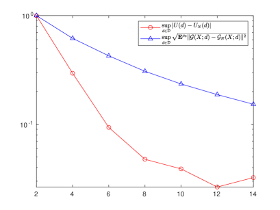
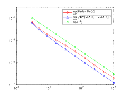
We have numerically evaluated both the uniform error EN:=supd𝒟|U(d)UN(d)|assignsubscript𝐸𝑁subscriptsupremum𝑑𝒟𝑈𝑑subscript𝑈𝑁𝑑E_{N}:=\sup_{d\in{\mathcal{D}}}|U(d)-U_{N}(d)| and the left-hand side term in inequality (27) with varying N𝑁N. For evaluating U(d)𝑈𝑑U(d) and UN(d)subscript𝑈𝑁𝑑U_{N}(d) we use trapezoidal rule for discretizing 𝒳𝒳\mathcal{X} using an equidistant grid with 251 nodes. For the data space 2superscript2\mathbb{R}^{2} we utilized Gauss–Hermite–Smolyak quadrature with 3843 nodes. For estimating ENsubscript𝐸𝑁E_{N} and the left-hand side of (27) we fix a 21×21212121\times 21 grid for the design space 𝒟𝒟{\mathcal{D}} over which we optimize. Moreover, for any d𝑑d we numerically solve 𝔼μ0𝒢(X;d)𝒢N(X;d)2superscript𝔼subscript𝜇0superscriptnorm𝒢𝑋𝑑subscript𝒢𝑁𝑋𝑑2\mathbb{E}^{\mu_{0}}\left\|{\mathcal{G}}(X;d)-{\mathcal{G}}_{N}(X;d)\right\|^{2} using midpoint rule for the expectation with an equidistant grid in 𝒳𝒳\mathcal{X} with 1001 nodes. The supreme norm is approximated by calculating the maximum value of the evaluations in the grid of 𝒟𝒟\mathcal{D}.

Refer to caption
Refer to caption
Refer to caption
Refer to caption
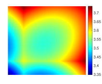
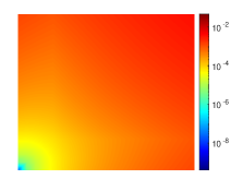
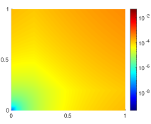
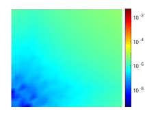
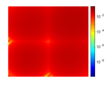
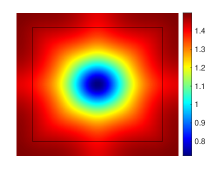
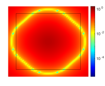
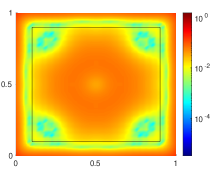
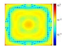
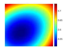
Figure 1: Convergence of the expected utility for example 5.1 is illustrated (evaluating in MATLAB using a grid of 21×21212121\times 21 for the design space 𝒟𝒟\mathcal{D}). The true utility U(d)𝑈𝑑U(d) is plotted w.r.t. d𝒟=[0,1]2𝑑𝒟superscript012d\in{\mathcal{D}}=[0,1]^{2} on the left upper corner. The approximation error |U(d)UN(d)|𝑈𝑑subscript𝑈𝑁𝑑|U(d)-U_{N}(d)| is plotted with N=9𝑁9N=9 (right upper corner), 333333 (left bottom corner) and 257257257 (right bottom corner). Smaller error towards the origin d1=d2=0subscript𝑑1subscript𝑑20d_{1}=d_{2}=0 is due to the linearity of 𝒢𝒢{\mathcal{G}} at this point.

In Figure 1 we have plotted the expected information gain U𝑈U and the errors |UNU|subscript𝑈𝑁𝑈|U_{N}-U| with values N=9,33𝑁933N=9,33 and 257257257. The errors ENsubscript𝐸𝑁E_{N} and supd𝒟𝔼μ0𝒢(X;d)𝒢N(X;d)2subscriptsupremum𝑑𝒟superscript𝔼subscript𝜇0superscriptnorm𝒢𝑋𝑑subscript𝒢𝑁𝑋𝑑2\sup_{d\in{\mathcal{D}}}\mathbb{E}^{\mu_{0}}\left\|{\mathcal{G}}(X;d)-{\mathcal{G}}_{N}(X;d)\right\|^{2} are plotted in Figure 2 for values varying between N=2𝑁2N=2 and N=103𝑁superscript103N=10^{3}. Moreover, we have also added the theoretical upper bound 𝒪(N2)𝒪superscript𝑁2{\mathcal{O}}(N^{-2}). We observe that the quantities have the same asymptotic behaviour following the theoretical bound.
Refer to caption
Figure 2: The convergence rate predicted by Theorem 3.4 is demonstrated for example 5.1. We plot the uniform errors of the expected utility (red curve) and uniform L2superscript𝐿2L^{2}-distance of the observation map and the surrogate with respect to the prior distribution (blue curve) with varying N𝑁N. For reference, a line proportional to N2superscript𝑁2N^{-2} is plotted.

5.2 Sparse piecewise linear interpolation in three dimensions

Consider the observation mapping 𝒢:[0,1]×𝒟2:𝒢01𝒟superscript2{\mathcal{G}}:[0,1]\times{\mathcal{D}}\to\mathbb{R}^{2} for 𝒟=[0.2,1]2𝒟superscript0.212{\mathcal{D}}=[0.2,1]^{2} defined by formula (25). In this subsection, we formulate a surrogate model 𝒢Nsubscript𝒢𝑁{\mathcal{G}}_{N} by interpolating data in both x𝑥x and d𝑑d variables. We apply a piecewise linear interpolation using a sparse grid with Clenshaw–Curtis configuration (Le Maître and Knio, 2010). Since 𝒢𝒢{\mathcal{G}} has continuous second partial derivatives on its domain, the error of this interpolation can be bounded by

𝒢𝒢NL(𝒳×𝒟)=𝒪(N2(logN)3(n1)),subscriptnorm𝒢subscript𝒢𝑁superscript𝐿𝒳𝒟𝒪superscript𝑁2superscript𝑁3𝑛1\|\mathcal{G}-\mathcal{G}_{N}\|_{L^{\infty}(\mathcal{X}\times\mathcal{D})}=\mathcal{O}(N^{-2}(\log N)^{3(n-1)}), (28)

where n=3𝑛3n=3 stands for the dimension of the domain, see e.g. (Barthelmann, Novak and Ritter, 2000; Novak and Ritter, 1996; Bungartz, 1998). For prior, we also assume here that the prior measure is a uniform distribution, μ0=𝒰(0,1)subscript𝜇0𝒰01\mu_{0}=\mathcal{U}(0,1). Following (27) we immediately observe

supd𝒟𝔼μ0𝒢(X;d)𝒢N(X;d)2=𝒪(N2(logN)6).subscriptsupremum𝑑𝒟superscript𝔼subscript𝜇0superscriptnorm𝒢𝑋𝑑subscript𝒢𝑁𝑋𝑑2𝒪superscript𝑁2superscript𝑁6\sup_{d\in{\mathcal{D}}}\sqrt{\mathbb{E}^{\mu_{0}}\left\|{\mathcal{G}}(X;d)-{\mathcal{G}}_{N}(X;d)\right\|^{2}}=\mathcal{O}(N^{-2}(\log N)^{6}). (29)

Similar to section 5.1 the mappings 𝒢𝒢{\mathcal{G}} and 𝒢Nsubscript𝒢𝑁{\mathcal{G}}_{N} are bounded and satisfy Assumption 4.1.
Refer to caption
Refer to caption
Refer to caption
Refer to caption
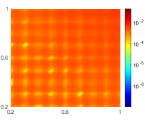
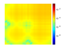
Figure 3: Convergence of the expected utility for example 5.2 is illustrated. The true utility U(d)𝑈𝑑U(d) is plotted w.r.t. d𝒟=[0.2,1]2𝑑𝒟superscript0.212d\in{\mathcal{D}}=[0.2,1]^{2} on the left upper corner. The approximation error |U(d)UN(d)|𝑈𝑑subscript𝑈𝑁𝑑|U(d)-U_{N}(d)| is plotted with N=18𝑁18N=18 (right upper corner), 108108108 (left bottom corner) and 632632632 (right bottom corner). Smaller error towards the origin d1=d2=0subscript𝑑1subscript𝑑20d_{1}=d_{2}=0 is due to the linearity of 𝒢𝒢{\mathcal{G}} at this point.

We again evaluate the difference EN:=supd𝒟|U(d)UN(d)|assignsubscript𝐸𝑁subscriptsupremum𝑑𝒟𝑈𝑑subscript𝑈𝑁𝑑E_{N}:=\sup_{d\in{\mathcal{D}}}|U(d)-U_{N}(d)| and the left-hand side term in inequality (29) with varying N𝑁N. In the same manner as the previous example, we estimated the expected information gains U(d)𝑈𝑑U(d) and UN(d)subscript𝑈𝑁𝑑U_{N}(d) using quadrature rules. For the integral over the space 𝒳𝒳\mathcal{X} we used again trapezoidal rule with 251 equidistant points, while for the space 𝒴𝒴\mathcal{Y} the Gauss–Hermite–Smolyak quadrature with 1730 nodes. For estimating ENsubscript𝐸𝑁E_{N} and the left-hand side of (27) we fix a 31×31313131\times 31 grid for the design space 𝒟𝒟{\mathcal{D}} over which we optimize. For constructing the surrogate we utilized the algorithm and toolbox detailed in (Klimke and Wohlmuth, 2005; Klimke, 2006). The supreme norm and the expectation with respect to the prior measure are estimated in the same way as the first example, the left-hand side of (29) is evaluated with a grid of 1001×31×31100131311001\times 31\times 31 nodes on 𝒳×𝒟𝒳𝒟\mathcal{X}\times\mathcal{D}.

Refer to caption
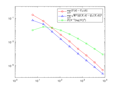
Figure 4: The convergence rate predicted by Theorem 3.4 is demonstrated for example 5.2. We plot the uniform errors of the expected utility (red curve) and the uniform L2superscript𝐿2L^{2}-distance of the observation map 𝒢𝒢{\mathcal{G}} and the surrogate 𝒢Nsubscript𝒢𝑁{\mathcal{G}}_{N} with respect to the prior distribution (blue curve) with varying N𝑁N. For reference, a curve proportional to N2(logN)6superscript𝑁2superscript𝑁6N^{-2}(\log N)^{6} is plotted.

Figure 3 plots the expected information gain U𝑈U and the errors |UNU|subscript𝑈𝑁𝑈|U_{N}-U| with values N=18,108𝑁18108N=18,108 and 632632632. Again, the errors ENsubscript𝐸𝑁E_{N} and supd𝒟𝔼μ0𝒢(X;d)𝒢N(X;d)2subscriptsupremum𝑑𝒟superscript𝔼subscript𝜇0superscriptnorm𝒢𝑋𝑑subscript𝒢𝑁𝑋𝑑2\sup_{d\in{\mathcal{D}}}\mathbb{E}^{\mu_{0}}\left\|{\mathcal{G}}(X;d)-{\mathcal{G}}_{N}(X;d)\right\|^{2} are plotted in Figure 4 for values varying between N=5𝑁5N=5 and N=104𝑁superscript104N=10^{4}. We observe that the numerical convergence rates of the error terms are of the same order while the theoretical upper bound also seems to align asymptotically with these rates asymptotically. After N=105𝑁superscript105N=10^{5} the convergence rates saturate around the value 107superscript10710^{-7} due to limited numerical precision of our implementation.

5.3 Optimal sensor placement for an inverse heat equation

Consider the heat equation on the domain Ω×𝒯=[0,1]2×[0,0.4]Ω𝒯superscript01200.4\Omega\times{\mathcal{T}}=[0,1]^{2}\times[0,0.4] with a source term S𝑆S with zero Neumann boundary condition and initial value according to

vtΔv𝑣𝑡Δ𝑣\displaystyle\frac{\partial v}{\partial t}-\Delta v =S(,x),absent𝑆𝑥\displaystyle=S(\cdot,x), (z,t)(0,1)2×𝒯𝑧𝑡superscript012𝒯\displaystyle(z,t)\in(0,1)^{2}\times\mathcal{T}
vn𝑣𝑛\displaystyle\nabla v\cdot n =0,absent0\displaystyle=0, (z,t)Ω×𝒯𝑧𝑡Ω𝒯\displaystyle(z,t)\in\partial\Omega\times\mathcal{T}
v(z,0)𝑣𝑧0\displaystyle v(z,0) =0,absent0\displaystyle=0, zΩ𝑧Ω\displaystyle z\in\Omega

where n𝑛n is a boundary normal vector. We assume that the source term is given by

S(z,t,x)={s2πh2exp(zx22h2),0t<τ,0,tτ.𝑆𝑧𝑡𝑥cases𝑠2𝜋superscript2superscriptnorm𝑧𝑥22superscript20𝑡𝜏0𝑡𝜏S(z,t,x)=\begin{cases}\frac{s}{2\pi h^{2}}\exp\left(-\frac{\left\|z-x\right\|^{2}}{2h^{2}}\right),&0\leq t<\tau,\\ 0,&t\geq\tau.\end{cases}

with parameter values s=2𝑠2s=2, h=0.050.05h=0.05 and τ=0.3𝜏0.3\tau=0.3. Moreover, the parameter x𝑥x is interpreted as the position of the source. We assume that we can observe v𝑣v at a location d𝒟:=[0.1,0.9]2Ω𝑑𝒟assignsuperscript0.10.92Ωd\in{\mathcal{D}}:=[0.1,0.9]^{2}\subset\Omega at predefined times tisubscript𝑡𝑖t_{i}, i=1,,5𝑖15i=1,...,5. The inverse problem in this setting is to estimate the source location x𝒳:=Ω𝑥𝒳assignΩx\in{\mathcal{X}}:=\Omega given the data y={v(d,ti)}i=155𝑦superscriptsubscript𝑣𝑑subscript𝑡𝑖𝑖15superscript5y=\{v(d,t_{i})\}_{i=1}^{5}\in\mathbb{R}^{5}, i.e., invert the mapping

𝒢:Ω×𝒟5,(x,d)y.:𝒢formulae-sequenceΩ𝒟superscript5maps-to𝑥𝑑𝑦{\mathcal{G}}:\Omega\times{\mathcal{D}}\to\mathbb{R}^{5},\quad(x,d)\mapsto y.

Here, we consider a Bayesian design problem with the aim to optimize the measurement location d𝑑d given a uniform prior of the source location x𝑥x on (0,1)2superscript012(0,1)^{2} and an additive Gaussian noise η𝒩(0,0.01I)similar-to𝜂𝒩00.01𝐼\eta\sim\mathcal{N}(0,0.01I) in the measurement.

Numerical implementation of 𝒢𝒢{\mathcal{G}} was carried out with a finite difference discretization for the spatial grid, while a fourth order backward differentiation was used for the temporal discretization. The surrogate observation mapping 𝒢Nsubscript𝒢𝑁{\mathcal{G}}_{N} is obtained by polynomial chaos expansion with Legendre polynomials. Here, we implemented the projection on an extended domain Ω×ΩΩΩ\Omega\times\Omega instead of Ω×𝒟Ω𝒟\Omega\times{\mathcal{D}} to avoid any potential boundary issues. The implementation follows (Huan and Marzouk, 2014) and more details can be found therein. In short, we define 𝒢Nsubscript𝒢𝑁{\mathcal{G}}_{N} as a sum of polynomials

𝒢N(x,d)=𝐣=0N𝒢𝐣Ψ𝐣(x,d),subscript𝒢𝑁𝑥𝑑superscriptsubscript𝐣0𝑁subscript𝒢𝐣subscriptΨ𝐣𝑥𝑑{\mathcal{G}}_{N}(x,d)=\sum_{{\bf j}=0}^{N}{\mathcal{G}}_{{\bf j}}\Psi_{{\bf j}}(x,d),

where 𝐣4𝐣superscript4{\bf j}\in{\mathbb{N}}^{4} and {Ψ𝐣}𝐣4subscriptsubscriptΨ𝐣𝐣superscript4\{\Psi_{{\bf j}}\}_{{\bf j}\in\mathbb{N}^{4}} are a Legendre polynomial basis in Ω×ΩΩΩ\Omega\times\Omega with the standard inner product, i.e. the L2superscript𝐿2L^{2}-inner product weighted by the uniform prior. Moreover, the coefficients satisfy

𝒢𝐣=Ω×Ω𝒢(x;d)Ψ𝐣(x,d)dxdyΩ×ΩΨ𝐣2(x,d)dxdy.subscript𝒢𝐣subscriptΩΩ𝒢𝑥𝑑subscriptΨ𝐣𝑥𝑑differential-d𝑥differential-d𝑦subscriptΩΩsuperscriptsubscriptΨ𝐣2𝑥𝑑differential-d𝑥differential-d𝑦{\mathcal{G}}_{{\bf j}}=\frac{\int_{\Omega\times\Omega}{\mathcal{G}}(x;d)\Psi_{{\bf j}}(x,d){\rm d}x{\rm d}y}{\int_{\Omega\times\Omega}\Psi_{{\bf j}}^{2}(x,d){\rm d}x{\rm d}y}. (30)

The parameter N𝑁N is the truncation level of the polynomial chaos. Notice carefully that we have included the design parameter d𝑑d in the approximation.

We compute the coefficients 𝒢𝐣subscript𝒢𝐣{\mathcal{G}}_{{\bf j}} with a Gauss–Legendre–Smolyak quadrature with Clenshaw-Curtis configuration with a high number (of the order 107superscript10710^{7}) of grid points and assume in the following that the truncation level N𝑁N is the dominating factor for the surrogate error supdΩ𝒢𝒢Nsubscriptsupremum𝑑Ωnorm𝒢subscript𝒢𝑁\sup_{d\in\Omega}\left\|{\mathcal{G}}-{\mathcal{G}}_{N}\right\|.

The utility functions were estimated as follows: for the integral over the data space 5superscript5\mathbb{R}^{5} we used the Gauss–Hermite–Smolyak quadrature with 117117117 nodes, while on the domain ΩΩ\Omega we implemented a bidimensional Clenshaw–Curtis–Smolyak quadrature with 768276827682 nodes. For the evaluation of maximal difference of the expected utility, we fixed an equidistant grid with 40×40404040\times 40 nodes in 𝒟𝒟\mathcal{D}. For evaluating the expectation in the term supd𝒟𝔼μ0𝒢(X;d)𝒢N(X;d)2subscriptsupremum𝑑𝒟superscript𝔼subscript𝜇0superscriptnorm𝒢𝑋𝑑subscript𝒢𝑁𝑋𝑑2\sup_{d\in{\mathcal{D}}}\mathbb{E}^{\mu_{0}}\left\|{\mathcal{G}}(X;d)-{\mathcal{G}}_{N}(X;d)\right\|^{2} we use midpoint rule and a grid of 252525 nodes in each direction on 𝒳𝒳\mathcal{X}. The supreme norm is approximated by calculating the maximum element of 25×25252525\times 25 nodes in a grid of 𝒟𝒟\mathcal{D}.

Refer to caption
Refer to caption
Refer to caption
Refer to caption
Figure 5: Convergence of the expected utility for Example 5.3 is illustrated. The true utility U(d)𝑈𝑑U(d) is plotted on the left upper corner. The approximation error |U(d)UN(d)|𝑈𝑑subscript𝑈𝑁𝑑|U(d)-U_{N}(d)| is plotted with N=2𝑁2N=2 (right upper corner), 666 (left bottom corner) and 141414 (right bottom corner). The design space 𝒟𝒟{\mathcal{D}} is highlighted with a black box.
Refer to caption
Figure 6: The convergence rate predicted by Theorem 3.4 is demonstrated for example 5.3. We plot the uniform errors of the expected utility (red curve) and the uniform L2superscript𝐿2L^{2}-distance of the observation map 𝒢𝒢{\mathcal{G}} and the polynomial chaos surrogate 𝒢Nsubscript𝒢𝑁{\mathcal{G}}_{N} with respect to the prior distribution (blue curve) with varying N𝑁N.

In Figure 5 we show the approximation of the utility functions for every polynomial degree. In both cases we can see a visual convergence with respect to the polynomial degree. In the spirit of previous examples, Figure 6 contains the errors between the surrogate models and the utility functions. Compared to the previous examples, the complexity of this computational task is substantially larger inducing larger numerical errors especially in the evaluation of ENsubscript𝐸𝑁E_{N}. Also, as is seen from Figure 5, the error close to the boundary of ΩΩ\Omega is converging substantially slower. However, as illustrated by Figure 6 the two rates of convergence are aligned with 𝒟𝒟{\mathcal{D}}.

6 Conclusion

We have developed a framework to study the stability of the expected information gain for optimal experimental designs in infinite-dimensional Bayesian inverse problems. We showed a uniform convergence for the expected information gain, with a sharp rate, given approximations of the likelihood. In the case of Bayesian inverse problems with Gaussian noise, this rate is proved to coincide with the L2superscript𝐿2L^{2}-convergence of the observation maps with respect to the prior distribution. Moreover, we also showed that the optimal design variable is also stable in the approximation. The results are illustrated by three numerical experiments.

Possible extensions of this work naturally include considering the stability of various other utilities such as the negative least square loss (Chaloner and Verdinelli, 1995) or utilities related to Bayesian optimization (Shahriari et al., 2015). Here, we only considered perturbations of the utility induced by a surrogate likelihood model. However, a further numerical (such as Monte Carlo based) approximation for the expected utility is most of the time needed. A number of results considering convergence with respect to Monte Carlo error for fixed design have been provided (see e.g. Ryan et al. (2016) and references therein) while the uniform case has not been addressed to the best of our knowledge. Finally, ΓΓ\Gamma-convergence does not directly provide a convergence rate for the optimal designs, which remains an interesting open problem.

{acks}

[Acknowledgments] The work of TH and DLD was supported by the Academy of Finland (decision numbers 326961 and 345720). JRRG was supported by the LUT Doctoral School.

References

  • Alexanderian (2021) {barticle}[author] \bauthor\bsnmAlexanderian, \bfnmAlen\binitsA. (\byear2021). \btitleOptimal experimental design for infinite-dimensional Bayesian inverse problems governed by PDEs: A review. \bjournalInverse Problems \bvolume37 \bpages043001. \endbibitem
  • Alexanderian, Gloor and Ghattas (2016) {barticle}[author] \bauthor\bsnmAlexanderian, \bfnmAlen\binitsA., \bauthor\bsnmGloor, \bfnmPhilip J\binitsP. J. and \bauthor\bsnmGhattas, \bfnmOmar\binitsO. (\byear2016). \btitleOn Bayesian A-and D-optimal experimental designs in infinite dimensions. \bjournalBayesian Analysis \bvolume11 \bpages671–695. \endbibitem
  • Alexanderian et al. (2014) {barticle}[author] \bauthor\bsnmAlexanderian, \bfnmAlen\binitsA., \bauthor\bsnmPetra, \bfnmNoemi\binitsN., \bauthor\bsnmStadler, \bfnmGeorg\binitsG. and \bauthor\bsnmGhattas, \bfnmOmar\binitsO. (\byear2014). \btitleA-optimal design of experiments for infinite-dimensional Bayesian linear inverse problems with regularized 0subscript0\ell_{0}-sparsification. \bjournalSIAM Journal on Scientific Computing \bvolume36 \bpagesA2122–A2148. \endbibitem
  • Alexanderian et al. (2016) {barticle}[author] \bauthor\bsnmAlexanderian, \bfnmAlen\binitsA., \bauthor\bsnmPetra, \bfnmNoemi\binitsN., \bauthor\bsnmStadler, \bfnmGeorg\binitsG. and \bauthor\bsnmGhattas, \bfnmOmar\binitsO. (\byear2016). \btitleA fast and scalable method for A-optimal design of experiments for infinite-dimensional Bayesian nonlinear inverse problems. \bjournalSIAM Journal on Scientific Computing \bvolume38 \bpagesA243–A272. \endbibitem
  • Barthelmann, Novak and Ritter (2000) {barticle}[author] \bauthor\bsnmBarthelmann, \bfnmVolker\binitsV., \bauthor\bsnmNovak, \bfnmErich\binitsE. and \bauthor\bsnmRitter, \bfnmKlaus\binitsK. (\byear2000). \btitleHigh dimensional polynomial interpolation on sparse grids. \bjournalAdvances in Computational Mathematics \bvolume12 \bpages273–288. \endbibitem
  • Beck et al. (2018) {barticle}[author] \bauthor\bsnmBeck, \bfnmJoakim\binitsJ., \bauthor\bsnmDia, \bfnmBen Mansour\binitsB. M., \bauthor\bsnmEspath, \bfnmLuis FR\binitsL. F., \bauthor\bsnmLong, \bfnmQuan\binitsQ. and \bauthor\bsnmTempone, \bfnmRaul\binitsR. (\byear2018). \btitleFast Bayesian experimental design: Laplace-based importance sampling for the expected information gain. \bjournalComputer Methods in Applied Mechanics and Engineering \bvolume334 \bpages523–553. \endbibitem
  • Beck et al. (2020) {barticle}[author] \bauthor\bsnmBeck, \bfnmJoakim\binitsJ., \bauthor\bsnmMansour Dia, \bfnmBen\binitsB., \bauthor\bsnmEspath, \bfnmLuis\binitsL. and \bauthor\bsnmTempone, \bfnmRaúl\binitsR. (\byear2020). \btitleMultilevel double loop Monte Carlo and stochastic collocation methods with importance sampling for Bayesian optimal experimental design. \bjournalInternational Journal for Numerical Methods in Engineering \bvolume121 \bpages3482–3503. \endbibitem
  • Braides (2002) {bbook}[author] \bauthor\bsnmBraides, \bfnmAndrea\binitsA. (\byear2002). \btitleGamma-convergence for Beginners \bvolume22. \bpublisherClarendon Press. \endbibitem
  • Bungartz (1998) {bbook}[author] \bauthor\bsnmBungartz, \bfnmH. J.\binitsH. J. (\byear1998). \btitleFinite Elements of Higher Order on Sparse Grids. \bseriesBerichte aus der Informatik. \bpublisherShaker. \endbibitem
  • Burger et al. (2021) {barticle}[author] \bauthor\bsnmBurger, \bfnmMartin\binitsM., \bauthor\bsnmHauptmann, \bfnmAndreas\binitsA., \bauthor\bsnmHelin, \bfnmTapio\binitsT., \bauthor\bsnmHyvönen, \bfnmNuutti\binitsN. and \bauthor\bsnmPuska, \bfnmJuha-Pekka\binitsJ.-P. (\byear2021). \btitleSequentially optimized projections in x-ray imaging. \bjournalInverse Problems \bvolume37 \bpages075006. \endbibitem
  • Chaloner and Verdinelli (1995) {barticle}[author] \bauthor\bsnmChaloner, \bfnmKathryn\binitsK. and \bauthor\bsnmVerdinelli, \bfnmIsabella\binitsI. (\byear1995). \btitleBayesian experimental design: A review. \bjournalStatistical Science \bpages273–304. \endbibitem
  • Da Prato and Zabczyk (2014) {bbook}[author] \bauthor\bsnmDa Prato, \bfnmGiuseppe\binitsG. and \bauthor\bsnmZabczyk, \bfnmJerzy\binitsJ. (\byear2014). \btitleStochastic equations in infinite dimensions. \bpublisherCambridge University Press. \endbibitem
  • Dal Maso (1993) {bbook}[author] \bauthor\bsnmDal Maso, \bfnmGianni\binitsG. (\byear1993). \btitleAn introduction to ΓΓ\Gamma-convergence \bvolume8. \bpublisherSpringer Science & Business Media. \endbibitem
  • Dashti and Stuart (2017) {bincollection}[author] \bauthor\bsnmDashti, \bfnmMasoumeh\binitsM. and \bauthor\bsnmStuart, \bfnmAndrew M\binitsA. M. (\byear2017). \btitleThe Bayesian approach to inverse problems. In \bbooktitleHandbook of uncertainty quantification \bpages311–428. \bpublisherSpringer. \endbibitem
  • Engl, Hanke and Neubauer (1996) {bbook}[author] \bauthor\bsnmEngl, \bfnmHeinz Werner\binitsH. W., \bauthor\bsnmHanke, \bfnmMartin\binitsM. and \bauthor\bsnmNeubauer, \bfnmAndreas\binitsA. (\byear1996). \btitleRegularization of inverse problems \bvolume375. \bpublisherSpringer Science & Business Media. \endbibitem
  • Foster et al. (2019) {barticle}[author] \bauthor\bsnmFoster, \bfnmAdam\binitsA., \bauthor\bsnmJankowiak, \bfnmMartin\binitsM., \bauthor\bsnmBingham, \bfnmElias\binitsE., \bauthor\bsnmHorsfall, \bfnmPaul\binitsP., \bauthor\bsnmTeh, \bfnmYee Whye\binitsY. W., \bauthor\bsnmRainforth, \bfnmThomas\binitsT. and \bauthor\bsnmGoodman, \bfnmNoah\binitsN. (\byear2019). \btitleVariational Bayesian optimal experimental design. \bjournalAdvances in Neural Information Processing Systems \bvolume32. \endbibitem
  • Garbuno-Inigo et al. (2023) {barticle}[author] \bauthor\bsnmGarbuno-Inigo, \bfnmAlfredo\binitsA., \bauthor\bsnmHelin, \bfnmTapio\binitsT., \bauthor\bsnmHoffmann, \bfnmFranca\binitsF. and \bauthor\bsnmHosseini, \bfnmBamdad\binitsB. (\byear2023). \btitleBayesian Posterior Perturbation Analysis with Integral Probability Metrics. \bjournalarXiv preprint arXiv:2303.01512. \endbibitem
  • Haber, Horesh and Tenorio (2008) {barticle}[author] \bauthor\bsnmHaber, \bfnmEldad\binitsE., \bauthor\bsnmHoresh, \bfnmLior\binitsL. and \bauthor\bsnmTenorio, \bfnmLuis\binitsL. (\byear2008). \btitleNumerical methods for experimental design of large-scale linear ill-posed inverse problems. \bjournalInverse Problems \bvolume24 \bpages055012. \endbibitem
  • Han and Atkinson (2009) {bbook}[author] \bauthor\bsnmHan, \bfnmWeimin\binitsW. and \bauthor\bsnmAtkinson, \bfnmKendall E\binitsK. E. (\byear2009). \btitleTheoretical numerical analysis: A functional analysis framework, 3rd edition. \bpublisherSpringer. \endbibitem
  • Helin, Hyvönen and Puska (2022) {barticle}[author] \bauthor\bsnmHelin, \bfnmTapio\binitsT., \bauthor\bsnmHyvönen, \bfnmNuutti\binitsN. and \bauthor\bsnmPuska, \bfnmJuha-Pekka\binitsJ.-P. (\byear2022). \btitleEdge-promoting adaptive Bayesian experimental design for X-ray imaging. \bjournalSIAM Journal on Scientific Computing \bvolume44 \bpagesB506–B530. \endbibitem
  • Herrmann, Schwab and Zech (2020) {barticle}[author] \bauthor\bsnmHerrmann, \bfnmLukas\binitsL., \bauthor\bsnmSchwab, \bfnmChristoph\binitsC. and \bauthor\bsnmZech, \bfnmJakob\binitsJ. (\byear2020). \btitleDeep neural network expression of posterior expectations in Bayesian PDE inversion. \bjournalInverse Problems \bvolume36 \bpages125011. \endbibitem
  • Huan and Marzouk (2013) {barticle}[author] \bauthor\bsnmHuan, \bfnmXun\binitsX. and \bauthor\bsnmMarzouk, \bfnmYoussef M\binitsY. M. (\byear2013). \btitleSimulation-based optimal Bayesian experimental design for nonlinear systems. \bjournalJournal of Computational Physics \bvolume232 \bpages288–317. \endbibitem
  • Huan and Marzouk (2014) {barticle}[author] \bauthor\bsnmHuan, \bfnmXun\binitsX. and \bauthor\bsnmMarzouk, \bfnmYoussef\binitsY. (\byear2014). \btitleGradient-based stochastic optimization methods in Bayesian experimental design. \bjournalInternational Journal for Uncertainty Quantification \bvolume4. \endbibitem
  • Kaipio and Somersalo (2006) {bbook}[author] \bauthor\bsnmKaipio, \bfnmJari\binitsJ. and \bauthor\bsnmSomersalo, \bfnmErkki\binitsE. (\byear2006). \btitleStatistical and computational inverse problems \bvolume160. \bpublisherSpringer Science & Business Media. \endbibitem
  • Klimke (2006) {barticle}[author] \bauthor\bsnmKlimke, \bfnmAndreas\binitsA. (\byear2006). \btitleSparse grid interpolation toolbox–User’s guide. \endbibitem
  • Klimke and Wohlmuth (2005) {barticle}[author] \bauthor\bsnmKlimke, \bfnmAndreas\binitsA. and \bauthor\bsnmWohlmuth, \bfnmBarbara\binitsB. (\byear2005). \btitleAlgorithm 847: spinterp: Piecewise multilinear hierarchical sparse grid interpolation in MATLAB. \bjournalACM Transactions on Mathematical Software (TOMS) \bvolume31 \bpages561–579. \endbibitem
  • Le Maître and Knio (2010) {bbook}[author] \bauthor\bsnmLe Maître, \bfnmOlivier\binitsO. and \bauthor\bsnmKnio, \bfnmOmar M\binitsO. M. (\byear2010). \btitleSpectral methods for uncertainty quantification: with applications to computational fluid dynamics. \bpublisherSpringer Science & Business Media. \endbibitem
  • Long, Motamed and Tempone (2015) {barticle}[author] \bauthor\bsnmLong, \bfnmQuan\binitsQ., \bauthor\bsnmMotamed, \bfnmMohammad\binitsM. and \bauthor\bsnmTempone, \bfnmRaúl\binitsR. (\byear2015). \btitleFast Bayesian optimal experimental design for seismic source inversion. \bjournalComputer Methods in Applied Mechanics and Engineering \bvolume291 \bpages123–145. \endbibitem
  • Long et al. (2015) {barticle}[author] \bauthor\bsnmLong, \bfnmQuan\binitsQ., \bauthor\bsnmScavino, \bfnmMarco\binitsM., \bauthor\bsnmTempone, \bfnmRaúl\binitsR. and \bauthor\bsnmWang, \bfnmSuojin\binitsS. (\byear2015). \btitleA Laplace method for under-determined Bayesian optimal experimental designs. \bjournalComputer Methods in Applied Mechanics and Engineering \bvolume285 \bpages849–876. \endbibitem
  • Marzouk, Najm and Rahn (2007) {barticle}[author] \bauthor\bsnmMarzouk, \bfnmYoussef M\binitsY. M., \bauthor\bsnmNajm, \bfnmHabib N\binitsH. N. and \bauthor\bsnmRahn, \bfnmLarry A\binitsL. A. (\byear2007). \btitleStochastic spectral methods for efficient Bayesian solution of inverse problems. \bjournalJournal of Computational Physics \bvolume224 \bpages560–586. \endbibitem
  • Nickl (2022) {barticle}[author] \bauthor\bsnmNickl, \bfnmRichard\binitsR. (\byear2022). \btitleBayesian non-linear statistical inverse problems. \bjournalLecture Notes ETH Zurich. \endbibitem
  • Novak and Ritter (1996) {barticle}[author] \bauthor\bsnmNovak, \bfnmErich\binitsE. and \bauthor\bsnmRitter, \bfnmKlaus\binitsK. (\byear1996). \btitleHigh dimensional integration of smooth functions over cubes. \bjournalNumerische Mathematik \bvolume75 \bpages79–97. \endbibitem
  • Pukelsheim (2006) {bbook}[author] \bauthor\bsnmPukelsheim, \bfnmFriedrich\binitsF. (\byear2006). \btitleOptimal design of experiments. \bpublisherSIAM. \endbibitem
  • Ruthotto, Chung and Chung (2018) {barticle}[author] \bauthor\bsnmRuthotto, \bfnmLars\binitsL., \bauthor\bsnmChung, \bfnmJulianne\binitsJ. and \bauthor\bsnmChung, \bfnmMatthias\binitsM. (\byear2018). \btitleOptimal experimental design for inverse problems with state constraints. \bjournalSIAM Journal on Scientific Computing \bvolume40 \bpagesB1080–B1100. \endbibitem
  • Ryan et al. (2016) {barticle}[author] \bauthor\bsnmRyan, \bfnmElizabeth G\binitsE. G., \bauthor\bsnmDrovandi, \bfnmChristopher C\binitsC. C., \bauthor\bsnmMcGree, \bfnmJames M\binitsJ. M. and \bauthor\bsnmPettitt, \bfnmAnthony N\binitsA. N. (\byear2016). \btitleA review of modern computational algorithms for Bayesian optimal design. \bjournalInternational Statistical Review \bvolume84 \bpages128–154. \endbibitem
  • Schillings and Schwab (2013) {barticle}[author] \bauthor\bsnmSchillings, \bfnmClaudia\binitsC. and \bauthor\bsnmSchwab, \bfnmChristoph\binitsC. (\byear2013). \btitleSparse, adaptive Smolyak quadratures for Bayesian inverse problems. \bjournalInverse Problems \bvolume29 \bpages065011. \endbibitem
  • Shahriari et al. (2015) {barticle}[author] \bauthor\bsnmShahriari, \bfnmBobak\binitsB., \bauthor\bsnmSwersky, \bfnmKevin\binitsK., \bauthor\bsnmWang, \bfnmZiyu\binitsZ., \bauthor\bsnmAdams, \bfnmRyan P\binitsR. P. and \bauthor\bsnmDe Freitas, \bfnmNando\binitsN. (\byear2015). \btitleTaking the human out of the loop: A review of Bayesian optimization. \bjournalProceedings of the IEEE \bvolume104 \bpages148–175. \endbibitem
  • Sprungk (2020) {barticle}[author] \bauthor\bsnmSprungk, \bfnmBjörn\binitsB. (\byear2020). \btitleOn the local Lipschitz stability of Bayesian inverse problems. \bjournalInverse Problems \bvolume36 \bpages055015. \endbibitem
  • Steinberg and Hunter (1984) {barticle}[author] \bauthor\bsnmSteinberg, \bfnmDavid M\binitsD. M. and \bauthor\bsnmHunter, \bfnmWilliam G\binitsW. G. (\byear1984). \btitleExperimental design: review and comment. \bjournalTechnometrics \bvolume26 \bpages71–97. \endbibitem
  • Stuart (2010) {barticle}[author] \bauthor\bsnmStuart, \bfnmAndrew M\binitsA. M. (\byear2010). \btitleInverse problems: a Bayesian perspective. \bjournalActa numerica \bvolume19 \bpages451–559. \endbibitem
  • Wu, Chen and Ghattas (2020) {barticle}[author] \bauthor\bsnmWu, \bfnmKeyi\binitsK., \bauthor\bsnmChen, \bfnmPeng\binitsP. and \bauthor\bsnmGhattas, \bfnmOmar\binitsO. (\byear2020). \btitleA fast and scalable computational framework for large-scale and high-dimensional Bayesian optimal experimental design. \bjournalarXiv preprint arXiv:2010.15196. \endbibitem