A Latent Space Model for Human Leukocyte Antigen Compatibility Networks in Kidney Transplantation

Abstract

Chronic Kidney Disease (CKD) affects 7-12$\%$ of the population worldwide[romagnani2017chronic] and may lead to end-stage renal disease (ESRD), which is defined as the irreversible loss of kidney function. Patients with ESRD require a kidney transplant, and insufficient kidney storage has been a critical problem for patients who require a kidney transplant. On the other hand, even successful kidney transplants will fail over time, and patients then require a replacement with another kidney transplant from a new donor[Scientific2018]. Prior research shows that the human leukocyte antigen(HLA) system is associated with graft loss in organ transplant; a donor-recipient HLA pair with higher compatibility is more likely to receive a longer transplant survival times[terasaki2004predicting]. In this paper, we propose a latent space model for the HLA compatibility network to predict HLA compatibilities between kidney donors and recipients, especially for those infrequently-observed or previously unobserved HLA pairs. Both donor and recipient HLA nodes are placed in a lower-dimensional latent space. We can induce donor and recipient relations through distances between nodes in the latent space; then, we estimate the latent positions using maximum a posterior probability (MAP) estimator. To evaluate our model, we hold out 10$\%$ of edge weights from the data set and attempt to predict them with our model. Our analysis reveals some agreement between the predicted and actual weights and indicates that our model could predict compatibilities for those infrequently-observed or previously unobserved HLA pairs.

1 Introduction

Chronic Kidney Disease (CKD) has been a common disease globally and can lead to end-stage renal disease (ESRD), which is defined as the irreversible loss of kidney function. There are two treatments for ESRD, kidney transplant and dialysis. A kidney transplant is more desirable than dialysis because it usually leads to a better quality of life and longer survival time than dialysis.

Despite the advantages of kidney transplants, most ESRD patients are treated with dialysis primarily because there is an insufficient number of compatible donors for patients[Scientific2018]. Moreover, kidney transplants inevitably fail over time, which is referred to as graft failure; patients with graft failure require a replacement with another kidney transplant. The median time to kidney graft failure was 9.8 years in 2008. If we could increase the time to kidney graft failure, patients could live longer without doing another transplant; it would delay patients who receive a transplanted kidney being put back on the waiting list, potentially reducing the number of patients every year.

During transplantation, the recipients’ immune system will launch an attack against the transplanted organ. High immunogenicity is associated with worse transplant outcomes, namely shorter graft survival time to transplant failure. The HLA system significantly affects clinical survival time for organ transplants. Thus, We could increase patients’ survival time by matching a better HLA compatible kidney[claas2004acceptable][konvalinka2015utility].

We first propose a data-driven approach to estimating HLA compatibilities by fitting a Cox proportional hazards (PH) model to the transplant database of over 60,000 kidney transplants. The coefficient in the Cox-PH model corresponds to the HLA compatibility. This approach is unable estimate HLA pairs for which we do not have many prior transplants. Therefore, we proposed a network-based approach to predict those infrequently-observed or previously unobserved HLA compatibilities.

In this paper, we use a bipartite network to express the relationship between kidney donor and recipient HLA coefficients, which we refer to as the HLA compatibility network. It has two node types, such that two nodes can be linked only if they are of different types. Here, one set of nodes represents the donor HLA nodes, and the other set of nodes represent the recipient HLA nodes. We then develop a latent space model which captures the features of different HLA types of donor and recipient. The latent space model allows us to visualize donor and recipient nodes in a lower-dimensional latent space, and in that space, distances between donor and recipient node express their HLA compatibilities. With such a latent space embedding, we could potentially predict HLA pairs that were unobserved before.

2 Background and Motivation

2.1 Chronic Kidney Disease

CKD, which is defined as the loss of kidney function from various sources such as urine abnormalities and structural abnormalities, is common throughout the world. In the US, 37 million adults have some form of CKD[denu2018potential], and it is the 9^th leading cause of death[heron2019deaths]. Moreover, patients with CKD are more likely to get cardiovascular disease and it can lead to the irreversible loss of kidney function, called ESRD. The prevalence of overall ESRD is between 7-12% in the world[webster2017chronic]. Treatment of ESRD requires either dialysis or kidney transplantation. Kidney transplants give significantly better quality of life, longer survival time, and are more cost-effective than dialysis. However, the barrier for transplantation is that the US’s storage of kidneys is severely insufficient. In 2014, around 100,000 people were waiting for a kidney in the US. Although the number of patients on the kidney transplant waiting list declined over the next four years and decrease to 92,000 in 2018, there are still many patients waiting for transplantation, and about 4500 candidates die or become too sick for transplant every year. This decline appeared to be due to further increases in deceased and living donor transplants, rather than the decline of new patients added to the waiting list. By contrast, the incidence of ESRD has been increasing over the years[denu2018potential]. Additionally, kidney transplants will fail over time, known as graft failure, and patients with graft failure will require another transplant and will be put back on the kidney transplant waiting list[hart2019optn]. Overall, ESRD has been a significant public health problem and economic burden[denu2018potential].

To solve the insufficient kidney supply, it is often impossible to control the number of kidney donors. A more practical approach would be to reduce the number of patients added to the kidney transplant waiting list. From 1994 to 2008, due to improvements in immunosuppression, the median survival time was increased from 8 to 10 years; this 2-year improvement in graft survival times saved roughly 17, 000 transplants per year with the same number of donors[hart2018optn]. Thus, improving graft survival time could lead to significant improvements for ESRD.

2.2 The Human Leukocyte Antigen System

A significant biological factor affecting the transplanted kidney’s clinical survival time is the compatibility between the kidney donor and recipient’s human leukocyte antigens. The HLA system is a system of proteins expressed on a transplant’s cell that recognizes the immunogenicity of a kidney transplant from a donor[hart2019optn][claas2004acceptable][konvalinka2015utility][malheiro2015analysis][lucia2015preformed][kosmoliaptsis2016alloantibody]. The HLA system includes three primary HLA loci, which are HLA-A, HLA-B, and HLA-DR. For each HLA locus, there are many different specific HLA proteins. The general way to express HLA antigens is using two-digit, or low-resolution typing, where each HLA is identified by ”HLA” followed by a hyphen, a letter indicating the locus, and a 1-digit or 2-digit number which indicates the HLA protein, e.g., HLA-A1 [shankarkumar2004human]. Each person has two sets of HLAs, one inherited from the father and one from the mother, and each set includes 1 from each locus; HLA-A, HLA-B, and HLA-DR[cecka1997pediatric]. Therefore, Each donor and recipient has six antigens, figure 1 shows an example of a pair of donor and recipient HLA antigens. The compatibility between HLAs of the kidney donor and recipient has been shown to be a significant factor affecting transplanted kidneys’ survival times. [opelz2017hla][claas2004acceptable][konvalinka2015utility]. A pair of kidney donors and recipients with higher HLA compatibility receive a higher possibility of getting a good transplant outcome.

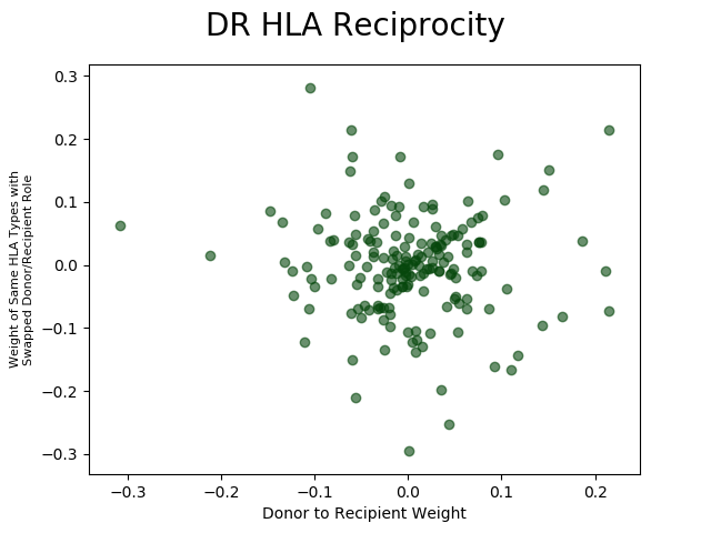
While the kidney transplant network is clearly a bipartite network, justification is needed for how the HLA compatibility network is represented. HLA compatibilities could more simply be represented as a unipartite network between types irrespective of donor or recipient. However, a major assumption required for this is that HLA types have the same compatibility to other types regardless of whether they are from a donor or recipient kidney. To show this assumption does not hold, figure 2 conveys that there is little to no correlation between the compatibility of an HLA type as a donor or as a recipient. Thus, it is necessary to represent the HLA compatibility network as bipartite.

Figure 1: An example of HLA antigens for a pair of donor and recipient

Figure 2: Plot showing the relationship of weights between pairs of HLA types when treated as a bipartite donor or recipient. The x-axis gives the donor to recipient weight of the pair while the y-axis gives the weight of the same pair when the donor type is instead treated as the recipient and vice versa.

2.3 Related Work

Network models are favored to represent relational information among interacting units. Hoff et al. first proposed the latent space approaches to many social network analysis in 2002. In their work, they developed a class of models where the probability of a relation between actors depends on individuals’ positions in an unobserved latent space. This method provides a visual and interpretable model-based spatial representation of social relationships[hoff2002latent]. Hoff’s approaches were extended by many researchers later on. Several latent space approaches have been proposed for bipartite networks[vasques2020latent][friel2016interlocking][sarkar2007latent]. Friel et al. develop a latent space model for dynamic bipartite networks that capture key features of interlocking directorships’ evolution over time. The model attaches latent positions in a low-dimensional space to each director and company. Their analysis reveals that the change of interlocking directorates’ level in Irish companies, as measured by a contraction of the latent space[friel2016interlocking]. Sarkar et al. ’s model are similar to Friel et al.’s, a dynamic adaptation of the latent space model for cooccurrence data. Sarkar et al. investigated the cooccurrence of words and authors in text corpora. It models the probability of cooccurrence of words and authors using the empirical distribution of word and author occurrences and reducing the distance between their latent positions[sarkar2007latent]. Similarly, in our model, donor and recipient nodes are placed in the same latent space. We model edge weights with a linear regression on the distance in the latent space, and our estimation is done to find the maximum a posterior (MAP) estimators of the unknown parameters and latent positions.

3 Methods and Technical Solutions

3.1 HLA compatibility network

The HLA coefficients between donor and recipient are estimated by an $\ell_{2}$-penalized Cox-PH model fitted to the transplant outcome data from the scientific registry of transplant recipients (SRTR) database[Scientific2018]. As mentioned before, we were able to express the HLA coefficients as a weighted bipartite network, namely the HLA compatibility network, with two types of nodes (donor and recipient nodes). Edges only ever link between nodes of different types. The edge value corresponds to the HLA compatibilities. An edge with high positive value represents high HLA compatibility between this donor and recipient pair and is likely to get a better outcome; an edge with low negative value represents low HLA compatibility and less likely to get a better outcome. We consider a network of HLA pairs for each locus separately; this results in three different networks. An example of a partial HLA-DR coefficients table and the corresponding HLA compatibility network are shown in figure 4 and 3. In this network, there is a previously unobserved edge DR2-DR1, marked as red dash line in the figure; our main objective is to predict this unobserved HLA edge value based on past observed edge outcomes. In the HLA compatibility network, we denote $W$ as the weighted matrix, and each entry $w_{ij}$ in the weighted matrix represents the edge weight value between donor node $i$ and recipient node $j$.

Figure 3: The partial HLA-DR coefficients table: the first row denotes donor HLA types, the first column denotes recipient HLA types and the red cell denotes missing value (previously unobserved HLA pair)

Figure 4: The partial HLA-DR compatibility network: the red dash edge denotes missing edge (previously unobserved HLA pair) in this network

3.2 Baseline Prediction Model

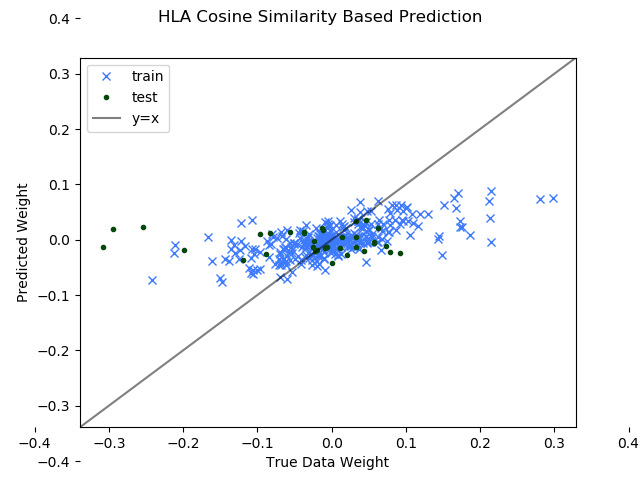
For comparison purposes, it is useful to have a relatively basic and interpretable model that gives a baseline with which to judge our latent space model. To this end, a simple model using weighted averages based on cosine similarity was chosen. Cosine similarity is the normalized dot product of two vectors. From the adjacency matrix of weights between donors and recipients, treating the rows or columns as vectors allows us to compute the cosine similarity between nodes on the same side of the bipartite network. We could treat the resulting cosine similarities as a unipartite network representing similarity amongst either donors or recipients, depending on whether rows or columns were treated as vectors. From this, missing bipartite links from a donor $d$ to a recipient $r$ were able to be predicted by taking the average of the weights of all known edges to $r$ weighted by the cosine similarity between $d$ and the respective edge’s donor. The resulting predictive power of this model can visually be seen in figure 5 by comparing the predictions to the known weights, judged by how closely they align with the line $y$=$x$ (representing perfect predictions). Evaluation criteria for this model averaged over 20 iterations of the train/test splits are shown in Table 1.

Figure 5: Predicted weights vs. actual weights from cosine similarity based model

Table 1: Evaluation of training and testing sets for cosine similarity based model (average over 20 train/test splits)

Train-R^2	Train-MSE	Test-R^2	Test-MSE
0.3597	0.0040	-0.1308	0.0062

3.3 Latent space methods

Within the context of the latent space model, donors and recipients’ node positions are embedded in the latent space where corresponds to features in the observed HLA network with higher edge nodes being put closer. Thus, the HLA network’s dependence could be induced through distances between nodes in the latent space. This method provides a highly intuitive interpretation of the HLA network.

In the donor-recipient latent space model, we let $z_{di}$ and $z_{rj}$ denote the $i^{th}$ donor node and the $j^{th}$ recipient node in the latent space. Let $N_{d}$ and $N_{r}$ be the number of donor nodes and recipient nodes. To model the latent positions, we first sample node positions from the standard Normal distribution with a zero mean and variance $\sigma^{2}$ multiplies a identity matrix $I_{k}$ where k is the dimension of latent space. For each donor and recipient node $i$ = 1,…,$N_{d}$, $j$ = 1,…,$N_{r}$, we have

(3.1) $$z_{d_{i}},z_{r_{j}}\sim Normal(0,\sigma_{z}^{2}I_{k})$$

This differs from Hoff’s model; we model the affinities - the relation of distances in the latent space and edge weights - using linear regression, rather than logistic regression. Then, the affinities between $i^{th}$ donor node and $j^{th}$ recipient node equal to a scalar $\alpha$ subtract by the distance in the latent space, where $\alpha$ and $\beta$ are scalar parameters, the equation of affinities are

(3.2) $$\eta_{ij}=\alpha-\beta*|z_{d_{i}}-z_{r_{j}}|$$

From affinities, weights are sampled from another Normal distribution with the affinities as mean and variance $\sigma_{w}^{2}$; then the weight between $i^{th}$ donor node and $j^{th}$ recipient node is

(3.3) $$w_{ij}\sim Normal(\eta_{ij},\sigma_{w}^{2})$$

Finally, we could perform maximum a posterior(MAP) to estimate model parameters using Edward, a probabilistic programming python library. MAP in Edward implements gradient-based optimization to solve the optimization problem. Each random variable will be implicitly optimized using ’PointMass’ random variable that is defined internally with constrained support, has unconstrained free parameters, and is initialized using standard Normal draws. Edward builds its loss function, differentiates the gradient, and finds an optima automatically[tran2016edward].

4 Empirical Evaluation

4.1 Simulation study

To make a pilot evaluation of our proposed model, we fit our model on a simulated network first. The advantage of running a simulated study is that we could start by simulating the latent positions and derive the weights from the latent positions. We could visually compare the actual latent embedding with the predicted latent embedding; however, we cannot compare this in the practical network because we cannot get the actual latent embedding for the HLA compatibility network.

We simulated a bipartite network with 20 nodes for each type, where $N_{d}$ and $N_{r}$ equal to 20. Their latent positions $z_{d}$ and $z_{r}$ were simulated from a standard Normal distribution. To make the structure easier, we set parameters $\alpha$ = 0 and $\beta$ = 1. Then simulated edge weights $w_{ij}$ can be derive from the equation

(4.4) $$w_{ij}=\alpha-\beta*|z_{d_{i}}-z_{r_{j}}|$$

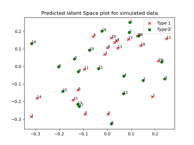
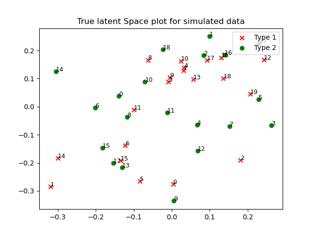
To evaluate the simulated study, we first hold 10 percent of simulated data as the testing set and use the rest 90 percent as the training set to fit our model. Figure 6 and figure 7 is the actual and the estimated latent space plot for the simulated network: we take a Procrustes’s transform[ross2004procrustes] for the estimated plot to make it in the same direction and scaling as the actual latent space embedding; it reveals the estimated plot is high matches the actual plot. We could then predict weights using an estimated latent space plot. We draw a comparison plot, as shown in figure 8; For each point, the x-axis represents the actual weight value, and the y-axis represents the predicted weight value. The black line, which is y = x, suggests that the actual value is equal to the predicted value. The scatter plot revels that our prediction value is close to the actual value - both training and testing set prediction are accurate. Overall, the latent plot and the scatter plot both indicate our model works ideally on the simulated network.

Figure 6: Actual latent space plot for simulated network: red cross and green circle denote two different types of nodes in latent space

Figure 7: Predicted latent space plot for simulated network: red cross and green circle denote two different types of nodes in latent space

Figure 8: Predicted weights vs. true weights on simulated network

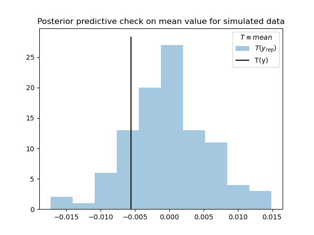
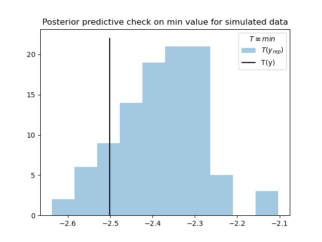
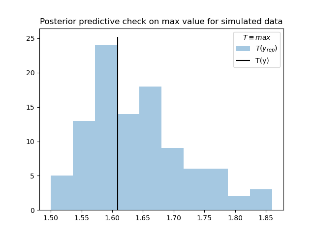
To assess our prediction, we could run a posterior predictive checks [gelman1996posterior] by simulating replicated data under the fitted model and then comparing these to the observed data. The check on the mean, minimum and maximum are shown in figure 9, 10 and 11. The vertical black line indicates the actual statistical variables (mean, minimum, and maximum) for the observed data, and the histogram represents the statistical variables’ distribution of 100 replicated data. The actual values (the vertical black line in the plot) for the observed data are mean: -0.0056, minimum: -2.5008, and maximum: 1.60884. As for the replicated data, we could calculate the average value for these three distribution, which are mean: -0.0029, minimum: -2.4393, and maximum: 1.6242. Results are accurate compared with the actual values. It indicates that our model gives valid predictions on the observed simulated data.

Figure 9: Posterior predictive check on mean value for simulated network

Figure 10: Posterior predictive check on min value for simulated network

Figure 11: Posterior predictive check on max value for simulated network

4.2 HLA compatibility network study

The HLA coefficients data were generated from a Cox-PH fitted to the transplant data set from the SRTR. Since we cannot evaluate the HLA combinations that were unobserved directly, we randomly hold out some of the HLA combinations we have seen before and temporarily hide those entries - 10$\%$ data held out as testing set; we then fit the latent space model to the rest of data - 90$\%$ data as the training set. We could estimate latent positions and plot the latent embedding to predict the hold-out values based on their latent space distance. Finally, we can evaluate the model behavior by comparing predicted hold-out values with the testing set.

Our observed model was trained based on different HLA loci separately. For each type of HLA locus, we have different HLA antigens. The number of antigens for types of HLA loci shown in table 2. Since the HLA-DR network has the least number of HLA combinations and missing values - about 4$\%$ data were missing, it would give us a more leisurely start to fit our proposed model to the HLA-DR network than HLA-A and HLA-B.

Table 2: Number of antigens for each HLA locus

# of types	HLA-A	HLA-B	HLA-DR
Donor	26	53	19
Recipient	26	54	19

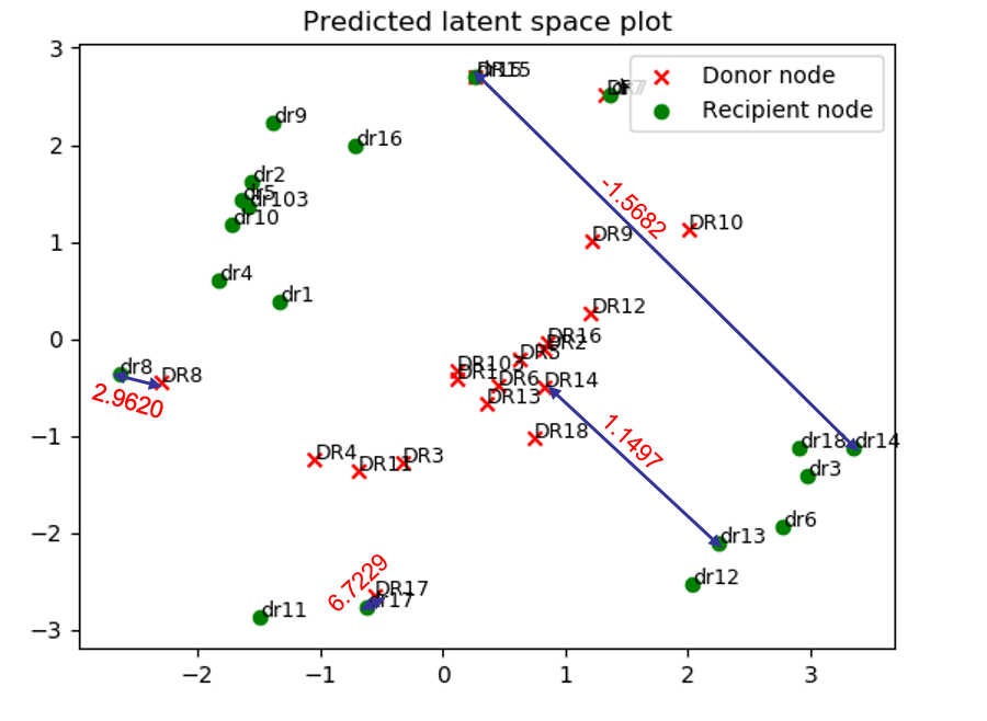
We could estimate and plot the latent space embedding by choosing the latent dimensions to 2. Figure 12 shows the latent space plot estimated from our model. The plot includes donor and recipient nodes (red cross points: donor nodes, green circle points: recipient nodes) for HLA-DR. As we talked earlier, a pair of donor and recipient node with a higher HLA compatibility tends to locate close in the latent space, e.g., donor node DR17 and recipient DR17 have relatively high compatibility: 6.7229, and they were placed pretty close in the latent space.

Figure 12: Predicted latent space plot for HLA network: four HLA pair coefficients are marked as example in this plot

Then we could predict HLA coefficients based on this latent space plot and compare it with the actual coefficients for both training and testing set. We could draw a comparison plot, as shown in figure 16. Each point in the figure denotes a coefficient of a donor-recipient pair (red cross points: training coefficient, green circle points: testing coefficient). For each point, the x-axis represents the actual coefficient, and the y-axis represents the predicted coefficient. The black line, which is y = x, suggests positions that the actual value is equal to the predicted value; in other words, a coefficient point that sits close to the black line indicates the predicted value is similar to the actual value. Although we could not conclude that the actual value and predicted value are giving exactly a good match in this figure, we could see the scatter points’ trend potentially have a positive linear correlation. To test that, we examine only the sign prediction. The percent of correctly predicted signs are 70.91$\%$ for the training set and 69.44$\%$ for the testing set, which is not bad. It indicates that we have some agreement here for our model but not accurate. One potential reason could be that the 2D latent space might not hold all nodes into correct positions.

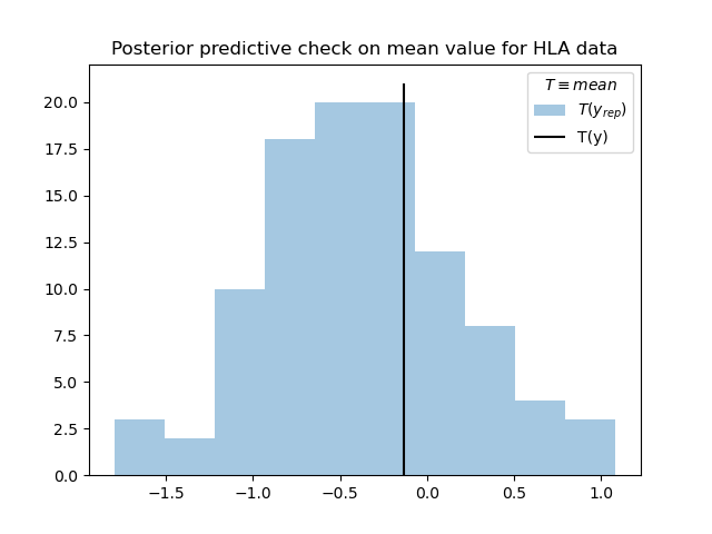
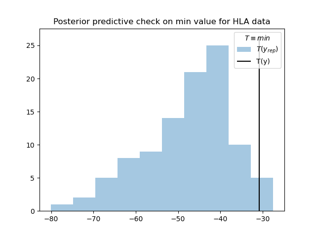
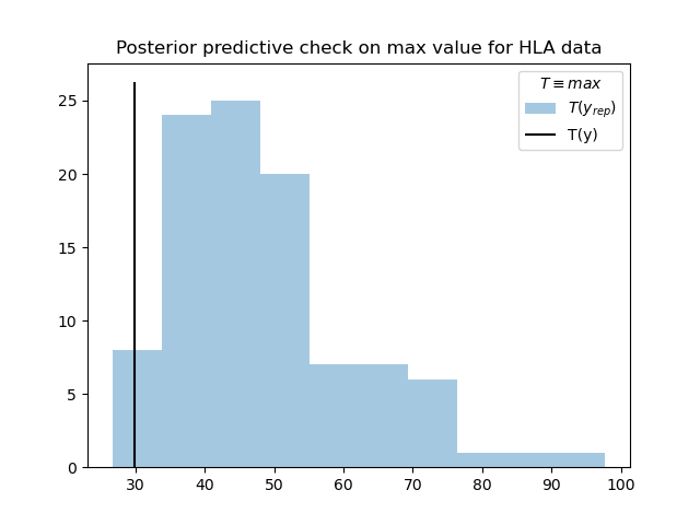
To assess our prediction, we could run the same posterior predictive check as the simulated network. The check on the mean, minimum and maximum are shown in figure 13, 14 and 15. The actual values (the vertical black line in the plot) for the HLA coefficients are mean: -0.1324, minimum: -30.8497, and maximum: 29.8854. We could see the predicted mean seems accurate compared to the actual mean, which has an average value: -0.3759. The minimum and maximum distribution has some deviations and shows to have a broader range than the actual values. The average value of the replicated minimum is -47.4866, and the maximum is 48.5562. It could be accepted because the actual value is also located in the range of the posterior distribution.

Figure 13: Posterior predictive check on mean value for HLA network

Figure 14: Posterior predictive check on min value for HLA network

Figure 15: Posterior predictive check on max value for HLA network

As in figure 12, it seems our model tries to bunches all the same type of nodes together to minimize the loss. To verify this idea, we increase our latent dimensions and get figure 17 and figure 18 - comparison plot in higher latent dimensions. With the dimensions increased, the prediction seems more accurate than 2D latent space. To get a more precise evaluation, we calculate the mean square error (MSE) and R² for both training and testing prediction, varying from different latent dimensions. Results of averaging 20 different hold-out pairs are shown in table 3. We could see that the training set’s prediction significantly improved with the number of latent dimensions increased, but there is no much descent change for the testing set. If we look at the sign prediction table, which is calculated by the mean of accuracy in 20 different hold-out pairs, as shown in table 4, we could conclude that both the training and testing accuracy for sign prediction increased as the latent dimension increase. With a higher latent dimension, we add more flexibility to the model and lead to a better prediction of our HLA coefficients. With sign prediction, we could predict whether a transplant tends to receive a good or bad outcome.

Table 3: Evaluation table for training and testing set as varying from different latent dimensions

Dim.	Train-R^2	Train-MSE	Test-R^2	Test-MSE
2	0.1741	52.0641	-0.0125	46.5739
3	0.3563	40.6329	-0.0051	44.4654
4	0.4560	34.3342	0.0397	42.4126
5	0.5370	29.2216	0.0107	43.2956
6	0.6107	24.5666	0.0005	44.0752
7	0.6693	20.8711	0.0366	42.3331
8	0.7245	17.3943	-0.1563	40.9898
9	0.7646	14.8471	0.0530	40.8297
10	0.7941	12.9931	0.1081	39.1015

Table 4: Sign prediction table for training and testing set as varying from different latent dimensions

Latent dimensions	Train-sign(%)	Test-sign(%)
2	67.15	57.48
3	71.16	62.36
4	75.45	63.66
5	77.75	62.03
6	81.52	65.81
7	84.21	67.45
8	87.06	71.22
9	89.00	71.44
10	90.51	72.05

Figure 16: Predicted weights vs.actual weights in 2D latent space

Figure 17: Predicted weights vs.actual weights in 5D latent space

Figure 18: Predicted weights vs.actual weights in 10D latent space

5 Significance and Impact

This project’s primary impact on society is the benefit to public health, especially for patients on the kidney transplant waiting list. From this project, we hope to extend the graft survival time of a kidney transplant by matching a compatible kidney to a patient who has ESRD. For every kidney transplant, a small improvement in transplant outcomes could lead to significant improvements in outcomes at the societal level. As we mentioned earlier, a 2-year improvement to the median survival time could reduce roughly 17, 000 transplants per year. It could reduce a considerable ratio of patients in the kidney transplant waiting list.

To predict the kidney survival time, we analyze the HLA compatibility, a significant factor affecting graft survival time, by fitting a Cox-PH model. This paper aims to predict those prior infrequent-observed or unobserved donor-recipient HLA pairs by fitting a donor-recipient latent space model. Latent space models are useful for understanding the mechanisms that operate in network formation and provide good visualization on interacting units. However, when it comes to biological network - the HLA compatibility network - latent space model, or other network models, is practically non-existent.

The HLA compatibility network is a signed weighted bipartite network. Our donor-recipient latent space model is an extension of the latent distance model proposed by Hoff et al. and primary focus on the bipartite structure. Our results indicate that we have some reasonable prediction between the predicted and actual weights; this indicates we could predict compatibilities even for those previously unobserved HLA pairs. The sign prediction test reveals that our model works well in predicting whether a transplant tends to have good or bad outcomes. On the other hand, we could raise the idea that network science approaches would also be appropriate in solving biological problems.