Growing Schrödinger’s cat states by local unitary time evolution of product states

Saverio Bocini Université Paris-Saclay, CNRS, LPTMS, 91405, Orsay, France    Maurizio Fagotti maurizio.fagotti@universite-paris-saclay.fr Université Paris-Saclay, CNRS, LPTMS, 91405, Orsay, France
Abstract

We envisage many-body systems that can be described by quantum spin-chain Hamiltonians with a trivial separable eigenstate. For generic Hamiltonians, such a state represents a quantum scar. We show that, typically, a macroscopically-entangled state naturally grows after a single projective measurement of just one spin in the quantum scar. Moreover, we identify a condition under which what is growing is a “Schrödinger’s cat state”. Our analysis does not reveal any particular requirement for the entangled state to develop, provided that the quantum scar does not minimise/maximise a local conservation law. We study two examples explicitly: systems described by generic Hamiltonians and a model that exhibits a U(1)𝑈1U(1) hidden symmetry. The latter can be reinterpreted as a 2-leg ladder in which the interactions along the legs are controlled by the local state on the other leg through transistor-like building blocks.

Quantum superpositions of two macroscopically distinct states, known as “Schrödinger’s cat states”, from the famous Gedankenexperiment proposed by Schrödinger in 1935 [1, 2], or also as “(generalized) GHZ states”, from the observation by Greenberger, Horne, and Zeilingerin [3] on quantum spin models escaping the original Bell’s inequalities [4], are precious for their broad applications, e.g., in quantum metrology and quantum computation, but rare and generally short-lived for their fragility under real experimental conditions (which include decoherence, noise, particle loss, etc.). Several protocols have been proposed to contain the latter problems [5, 6, 7, 8, 9, 10, 11, 12, 13] and some of them have been experimentally realised [14, 15, 16, 17]. While such an instability undermines applications, it is, in fact, the defining feature of cat states, or, more generally, of states with extensive multipartite entanglement [18]. These are somehow unnatural states of matter in which fundamental physical properties such as cluster decomposition are lost. Engineering a cat state requires therefore a lot of control of the system, which, in turn, results in fine-tuned protocols designed with the clear goal of generating such exceptional states.

We propose a theoretical protocol that stands out for its naturalness, in the sense that the growth of macroscopic entanglement is a manifestation of an intriguing physical phenomenon rather than of clever manipulations of a system. The most general system that we consider is described by a quantum spin-1212\frac{1}{2} chain Hamiltonian 𝐇𝐇\boldsymbol{\mathbf{H}} with local interactions and a trivial separable eigenstate. Without loss of generality, the latter can be set equal to

|Ψ(0)=||,ketΨ0ketketabsentabsent\ket{\Psi(0)}=\ket{\Uparrow}\equiv\ket{\uparrow\cdots\uparrow}\,, (1)

where |ket\ket{\uparrow} denotes the eigenvector of the Pauli matrix σzsuperscript𝜎𝑧\sigma^{z} with eigenvalue 111 and \Uparrow will represent in this paper a generic number of adjacent \uparrow. Often the presence of such a trivial eigenstate is a consequence of a U(1)𝑈1U(1) symmetry, e.g., the conservation of 𝐒z=12𝝈zsuperscript𝐒𝑧12subscriptsuperscriptsubscript𝝈𝑧\boldsymbol{\mathbf{S}}^{z}=\frac{1}{2}\sum_{\ell}\boldsymbol{\mathbf{\sigma}}_{\ell}^{z}, where 𝝈αsuperscriptsubscript𝝈𝛼\boldsymbol{\mathbf{\sigma}}_{\ell}^{\alpha} are local operators acting like the Pauli matrices σαsuperscript𝜎𝛼\sigma^{\alpha} on site \ell and like the identity elsewhere. As we will see before long, the most interesting cases are however those in which 𝐒zsuperscript𝐒𝑧\boldsymbol{\mathbf{S}}^{z} is not conserved. If there are no additional relevant conserved operators, either |ket\ket{\Uparrow} is the ground state or it is an exact quantum scar [19, 20, 21]: its properties contrast with those of the eigenstates with similar energy. Quantum scars have recently attracted a lot of attention [22, 23, 24], also in connection with their unusual entanglement properties, displaying low bipartite entanglement, still potentially featuring extensive multipartite entanglement [25]. In our case the quantum scar is exceptional, as it is fully separable.

The basic idea is that the quantum scar is essentially metastable and could be transmuted into a state with extensive multipartite entanglement just by a local perturbation. Specifically, we consider the effect of a quantum measurement of a spin in a tilted direction with respect to z𝑧z, so that the state is projected into

|Ψθ(0+)=eiθ𝝈0y|=cosθ|+sinθ|ketsubscriptΨ𝜃superscript0superscript𝑒𝑖𝜃superscriptsubscript𝝈0𝑦ket𝜃ket𝜃ket\ket{\Psi_{\theta}(0^{+})}=e^{i\theta\boldsymbol{\mathbf{\sigma}}_{0}^{y}}\ket{\Uparrow}=\cos\theta\ket{\Uparrow}+\sin\theta\ket{\Uparrow\downarrow\Uparrow} (2)

with probability cos2θsuperscript2𝜃\cos^{2}\theta. Time evolution affects only the second term on the right hand side of Eq. [2], hence

|Ψθ(t)=cosθ|+sinθei𝐇t|,t>0.formulae-sequenceketsubscriptΨ𝜃𝑡𝜃ket𝜃superscript𝑒𝑖𝐇𝑡ket𝑡0\ket{\Psi_{\theta}(t)}=\cos\theta\ket{\Uparrow}+\sin\theta e^{-i\boldsymbol{\mathbf{H}}t}\ket{\Uparrow\downarrow\Uparrow},\quad t>0\,. (3)

The Lieb-Robinson bounds [26] ensure that the perturbation is irrelevant outside a light cone emerging from the space-time point of the measurement. Since the state before the measurement is an eigenstate, the measurement triggers a nontrivial time evolution only within a region whose length grows linearly with the time. Hence, neglecting the part of the system outside that region does not significantly affect the purity of the state. We call Ωϵ(t)subscriptΩitalic-ϵ𝑡\Omega_{\epsilon}(t) the smallest subsystem that contains the spin that is measured and that, as clarified later, can be considered pure at time t𝑡t with accuracy 1ϵ1italic-ϵ1-\epsilon. In the following, most of our considerations, including the use of terms such as “macroscopic” and “extensive”, will be referred to subsystem Ωϵ(t)subscriptΩitalic-ϵ𝑡\Omega_{\epsilon}(t). This allows us to treat on the same footing infinite systems, which are arguably more interesting from a theoretical point of view, and finite ones (provided that the actual system’s size is larger than Ωϵ(t)subscriptΩitalic-ϵ𝑡\Omega_{\epsilon}(t)), which are instead more relevant for the experiments. The situation is pictorially described in Fig. 1: after the spin flip at the origin, the component |ket\ket{\Uparrow\downarrow\Uparrow} of the state evolves in time, while the component |ket\ket{\Uparrow} stays constant; the effective size of the system is given by the spins that are inside the light cone originating from the local perturbation, while the rest of the spins are neglected.

First we show that, quite generally, in the settings considered the perturbation has everlasting effects on the expectation values of local observables arbitrarily far from the position of the measurement. That is to say, ei𝐇t||Ψπ/2(t)superscript𝑒𝑖𝐇𝑡ketketsubscriptΨ𝜋2𝑡e^{-i\boldsymbol{\mathbf{H}}t}\ket{\Uparrow\downarrow\Uparrow}\equiv\ket{\Psi_{\pi/2}(t)} is macroscopically different from |ket\ket{\Uparrow}, hence there exists an observable 𝐀=𝐚𝐀subscriptsubscript𝐚\boldsymbol{\mathbf{A}}=\sum_{\ell}\boldsymbol{\mathbf{a}}_{\ell}, where 𝐚subscript𝐚\boldsymbol{\mathbf{a}}_{\ell} are finite-support observables, such that |𝐀|Ψπ/2(t)|𝐀|Ψπ/2(t)quantum-operator-product𝐀quantum-operator-productsubscriptΨ𝜋2𝑡𝐀subscriptΨ𝜋2𝑡\braket{\Uparrow}{\boldsymbol{\mathbf{A}}}{\Uparrow}-\braket{\Psi_{\pi/2}(t)}{\boldsymbol{\mathbf{A}}}{\Psi_{\pi/2}(t)} is extensive, i.e., it scales linearly with the (effective) system size |Ωϵ(t)|subscriptΩitalic-ϵ𝑡|\Omega_{\epsilon}(t)| [27]. Such an effect is already remarkable, as, generally, local perturbations in quantum many-body systems either fade away or remain localised. We take it as the starting point of our investigation into the multipartite entanglement properties of |Ψθ(t)ketsubscriptΨ𝜃𝑡\ket{\Psi_{\theta}(t)}. We remind the reader that a state is said to have extensive multipartite entanglement if and only if the variance scales as the square of the system’s length for at least one extensive operator [28, 29, 30]. Being |Ψπ/2(t)ketsubscriptΨ𝜋2𝑡\ket{\Psi_{\pi/2}(t)} macroscopically different from |ket\ket{\Uparrow}, the reader is already in the position to infer that the projective measurement on the quantum scar |ket\ket{\Uparrow} will generate a state with extensive multipartite entanglement. But the situation is even more interesting. We provide evidence and then conjecture that, if the model has a hidden U(1)𝑈1U(1) symmetry (see below for the definition), |Ψπ/2(t)ketsubscriptΨ𝜋2𝑡\ket{\Psi_{\pi/2}(t)} is not macroscopically entangled; under those conditions, the projective measurement generates a genuine Schrödinger cat’s state consisting of an (ideally) arbitrarily large number of sites.

Refer to caption
Figure 1: Cartoon of the protocol. The state with a single spin down time evolves into a state that is macroscopically different from the pre-measurement state. If its fluctuations remain ordinary, the resulting superposition is a Schrödinger’s cat state. The scissors represent the fact that we ignore the region outside Ωϵ(t)subscriptΩitalic-ϵ𝑡\Omega_{\epsilon}(t).

1 The system

We investigate a variety of Hamiltonians with local densities. Our requirement of |ket\ket{\Uparrow} being eigenstate of the Hamiltonian allows for any kind of interactions that commute with the total spin in the z𝑧z direction, 𝐒z=12𝝈zsuperscript𝐒𝑧12subscriptsubscriptsuperscript𝝈𝑧\boldsymbol{\mathbf{S}}^{z}=\frac{1}{2}\sum_{\ell}\boldsymbol{\mathbf{\sigma}}^{z}_{\ell}, (such as the hopping term 𝝈x𝝈+nx+𝝈y𝝈+nysuperscriptsubscript𝝈𝑥superscriptsubscript𝝈𝑛𝑥superscriptsubscript𝝈𝑦superscriptsubscript𝝈𝑛𝑦\boldsymbol{\mathbf{\sigma}}_{\ell}^{x}\boldsymbol{\mathbf{\sigma}}_{\ell+n}^{x}+\boldsymbol{\mathbf{\sigma}}_{\ell}^{y}\boldsymbol{\mathbf{\sigma}}_{\ell+n}^{y} or the longitudinal Dzyaloshinskii–Moriya interaction 𝝈x𝝈+ny𝝈y𝝈+nxsuperscriptsubscript𝝈𝑥superscriptsubscript𝝈𝑛𝑦superscriptsubscript𝝈𝑦superscriptsubscript𝝈𝑛𝑥\boldsymbol{\mathbf{\sigma}}_{\ell}^{x}\boldsymbol{\mathbf{\sigma}}_{\ell+n}^{y}-\boldsymbol{\mathbf{\sigma}}_{\ell}^{y}\boldsymbol{\mathbf{\sigma}}_{\ell+n}^{x}) but not only that. The constraint is much weaker than a U(1)𝑈1U(1) symmetry and the Hamiltonian density can feature any term of the form 𝟏𝝈z2𝐎𝟏𝝈z21superscriptsubscript𝝈𝑧2subscript𝐎1superscriptsubscript𝝈𝑧2\frac{\boldsymbol{\mathbf{1}}-\boldsymbol{\mathbf{\sigma}}_{\ell}^{z}}{2}\boldsymbol{\mathbf{O}}_{\ell}\frac{\boldsymbol{\mathbf{1}}-\boldsymbol{\mathbf{\sigma}}_{\ell}^{z}}{2}, where 𝐎subscript𝐎\boldsymbol{\mathbf{O}}_{\ell} is a local operator with support in a region around \ell. Among the allowed operators, those with a hidden U(1)𝑈1U(1) symmetry (such as 𝝈1x(𝟏𝝈z)𝝈+1xsuperscriptsubscript𝝈1𝑥1superscriptsubscript𝝈𝑧superscriptsubscript𝝈1𝑥\boldsymbol{\mathbf{\sigma}}_{\ell-1}^{x}(\boldsymbol{\mathbf{1}}-\boldsymbol{\mathbf{\sigma}}_{\ell}^{z})\boldsymbol{\mathbf{\sigma}}_{\ell+1}^{x} or 𝝈1x(𝝈x𝝈+1x+𝝈y𝝈+1y)𝝈+2xsuperscriptsubscript𝝈1𝑥superscriptsubscript𝝈𝑥superscriptsubscript𝝈1𝑥superscriptsubscript𝝈𝑦superscriptsubscript𝝈1𝑦superscriptsubscript𝝈2𝑥\boldsymbol{\mathbf{\sigma}}_{\ell-1}^{x}(\boldsymbol{\mathbf{\sigma}}_{\ell}^{x}\boldsymbol{\mathbf{\sigma}}_{\ell+1}^{x}+\boldsymbol{\mathbf{\sigma}}_{\ell}^{y}\boldsymbol{\mathbf{\sigma}}_{\ell+1}^{y})\boldsymbol{\mathbf{\sigma}}_{\ell+2}^{x}) will play a special role.

1.1 Hidden U(1)𝑈1U(1) symmetry

The first class of Hamiltonians we consider has recently sparked some attention because it describes systems that are macroscopically sensitive to local perturbations [31, 32]. Such a sensitivity is triggered by so-called “semilocal conservation laws”, whose densities act as local observables only in a restricted space of operators with a particular symmetry. This unusual property could seem, at first glance, innocuous, but it allows the state to retain memory of so-called “string order” [33, 34, 35], making in turn symmetry-protected topological order survive the limit of infinite time [32]. An example of operator with a semilocal density in a system that is symmetric under the spin flip 𝝈x,y𝝈x,ysuperscriptsubscript𝝈𝑥𝑦superscriptsubscript𝝈𝑥𝑦\boldsymbol{\mathbf{\sigma}}_{\ell}^{x,y}\rightarrow-\boldsymbol{\mathbf{\sigma}}_{\ell}^{x,y} is

𝐒~z=12𝚷z(),superscript~𝐒𝑧12subscriptsuperscript𝚷𝑧\tilde{\boldsymbol{\mathbf{S}}}^{z}=\frac{1}{2}\sum_{\ell}\boldsymbol{\mathbf{\Pi}}^{z}(\ell)\,, (4)

where 𝚷z()superscript𝚷𝑧\boldsymbol{\mathbf{\Pi}}^{z}(\ell) can be thought of as a semi-infinite string of 𝝈zsuperscript𝝈𝑧\boldsymbol{\mathbf{\sigma}}^{z} and is such that [𝚷z()]2=𝐈superscriptdelimited-[]superscript𝚷𝑧2𝐈[\boldsymbol{\mathbf{\Pi}}^{z}(\ell)]^{2}=\boldsymbol{\mathbf{I}}, [𝚷z(),𝝈jz]=0superscript𝚷𝑧superscriptsubscript𝝈𝑗𝑧0[\boldsymbol{\mathbf{\Pi}}^{z}(\ell),\boldsymbol{\mathbf{\sigma}}_{j}^{z}]=0 and 𝚷z()𝝈jx,y=sgn(j12)𝝈jx,y𝚷z()superscript𝚷𝑧superscriptsubscript𝝈𝑗𝑥𝑦sgn𝑗12superscriptsubscript𝝈𝑗𝑥𝑦superscript𝚷𝑧\boldsymbol{\mathbf{\Pi}}^{z}(\ell)\boldsymbol{\mathbf{\sigma}}_{j}^{x,y}=\mathrm{sgn}(\ell-j-\frac{1}{2})\boldsymbol{\mathbf{\sigma}}_{j}^{x,y}\boldsymbol{\mathbf{\Pi}}^{z}(\ell). In spin-flip invariant settings, the density 𝚷z()superscript𝚷𝑧\boldsymbol{\mathbf{\Pi}}^{z}(\ell) of 𝐒~zsuperscript~𝐒𝑧\tilde{\boldsymbol{\mathbf{S}}}^{z} is a local observable and, if 𝐒~zsuperscript~𝐒𝑧\tilde{\boldsymbol{\mathbf{S}}}^{z} commutes with the Hamiltonian, it has important consequences on the evolution of the system, similarly to any other local conservation law — we refer the reader to Ref. [32] for additional details.

The (two) symmetry sectors of the spin-flip symmetry are connected by any odd local operator, e.g., 𝝈jxsuperscriptsubscript𝝈𝑗𝑥\boldsymbol{\mathbf{\sigma}}_{j}^{x}. Acting with it on the state splits the latter in two parts where the expectation value of semilocal operators takes opposite signs. This is at the origin of the macroscopic effects of local perturbations pointed out in Ref. [31]. The behaviour of fluctuations in these systems has not yet been investigated but the sensitivity of local observables to a single spin flip is a strong indication that the quantum measurement of a local observable such as 𝝈jxsuperscriptsubscript𝝈𝑗𝑥\boldsymbol{\mathbf{\sigma}}_{j}^{x} could result in macroscopically entangled states. As a specific example, we consider the following Hamiltonian

𝐇1=𝟏𝝈z8[J𝝈1𝑆𝝈+1++D(𝝈1×𝝈+1)]h2𝝈subscript𝐇1subscript1superscriptsubscript𝝈𝑧8delimited-[]𝐽subscript𝝈1𝑆subscript𝝈1𝐷subscript𝝈1subscript𝝈12subscript𝝈\boldsymbol{\mathbf{H}}_{1}=\sum_{\ell}\frac{\boldsymbol{\mathbf{1}}-\boldsymbol{\mathbf{\sigma}}_{\ell}^{z}}{8}[J\vec{\boldsymbol{\mathbf{\sigma}}}_{\ell-1}\overset{S}{\cdot}\vec{\boldsymbol{\mathbf{\sigma}}}_{\ell+1}+\\ +\vec{D}\cdot(\vec{\boldsymbol{\mathbf{\sigma}}}_{\ell-1}\times\vec{\boldsymbol{\mathbf{\sigma}}}_{\ell+1})]-\frac{\vec{h}}{2}\cdot\vec{\boldsymbol{\mathbf{\sigma}}}_{\ell} (5)

where a𝑆b=a(Sb)𝑎𝑆𝑏𝑎𝑆𝑏\vec{a}\overset{S}{\cdot}\vec{b}=\vec{a}\cdot(S\vec{b}). This Hamiltonian commutes with the semilocal charge 𝐒~zsuperscript~𝐒𝑧\tilde{\boldsymbol{\mathbf{S}}}^{z} — Eq. [4] — provided that

S=[1+γ2w0w1γ2000Δ]D=[00Dz]h=[00hz].formulae-sequence𝑆matrix1𝛾2𝑤0𝑤1𝛾2000Δformulae-sequence𝐷matrix00superscript𝐷𝑧matrix00superscript𝑧S=\begin{bmatrix}\frac{1+\gamma}{2}&w&0\\ w&\frac{1-\gamma}{2}&0\\ 0&0&\Delta\end{bmatrix}\quad\vec{D}=\begin{bmatrix}0\\ 0\\ D^{z}\end{bmatrix}\quad\vec{h}=\begin{bmatrix}0\\ 0\\ h^{z}\end{bmatrix}\,. (6)

It describes a system that can be interpreted as a quantum transistor chain, in which the building blocks 𝐓αβ=𝝈1α𝐈𝝈z2𝝈+1βsubscriptsuperscript𝐓𝛼𝛽superscriptsubscript𝝈1𝛼𝐈superscriptsubscript𝝈𝑧2superscriptsubscript𝝈1𝛽\boldsymbol{\mathbf{T}}^{\alpha\beta}_{\ell}=\boldsymbol{\mathbf{\sigma}}_{\ell-1}^{\alpha}\frac{\boldsymbol{\mathbf{I}}-\boldsymbol{\mathbf{\sigma}}_{\ell}^{z}}{2}\boldsymbol{\mathbf{\sigma}}_{\ell+1}^{\beta}, with (α,β){(x,x),(x,y),(y,x),(y,y),(z,z),(0,0)}𝛼𝛽𝑥𝑥𝑥𝑦𝑦𝑥𝑦𝑦𝑧𝑧00(\alpha,\beta)\in\{(x,x),(x,y),(y,x),(y,y),(z,z),(0,0)\} (𝝈0𝟏subscriptsuperscript𝝈01\boldsymbol{\mathbf{\sigma}}^{0}_{\ell}\equiv\boldsymbol{\mathbf{1}}), commute with 𝐒~zsuperscript~𝐒𝑧\tilde{\boldsymbol{\mathbf{S}}}^{z} — see Fig. 2.

Refer to caption
Figure 2: Pictorial representation of the quantum transistor chain, constructed as a sequence of building blocks 𝐓αβ=𝝈1α𝐈𝝈z2𝝈+1βsubscriptsuperscript𝐓𝛼𝛽superscriptsubscript𝝈1𝛼𝐈superscriptsubscript𝝈𝑧2superscriptsubscript𝝈1𝛽\boldsymbol{\mathbf{T}}^{\alpha\beta}_{\ell}=\boldsymbol{\mathbf{\sigma}}_{\ell-1}^{\alpha}\frac{\boldsymbol{\mathbf{I}}-\boldsymbol{\mathbf{\sigma}}_{\ell}^{z}}{2}\boldsymbol{\mathbf{\sigma}}_{\ell+1}^{\beta}.

It is known that 𝐇1subscript𝐇1\boldsymbol{\mathbf{H}}_{1} has infinitely many conserved operators with quasilocal [36] or semilocal [32] densities in the following regions of the parameter space:

  1. 1.

    If the only nonzero coupling constants are J𝐽J, γ𝛾\gamma, and hzsuperscript𝑧h^{z}, and γ=±1𝛾plus-or-minus1\gamma=\pm 1, the model is dual to the (integrable) Heisenberg XXZ one [37, 31];

  2. 2.

    If the only nonzero coupling constants are J𝐽J, ΔΔ\Delta, and hzsuperscript𝑧h^{z}, the model belongs to the family of hard-rod deformations of XXZ studied in Ref. [38]. In particular, for Δ=0Δ0\Delta=0 it is a special case of the Bariev model [39] and was recently dubbed “dual folded XXZ” [37]. These are special integrable models exhibiting Hilbert-space fragmentation and quantum jamming [37, 40, 41, 42].

For the first family of integrable models, Ref. [31] has already shown that a subsystem of |Ψπ/2(t)ketsubscriptΨ𝜋2𝑡\ket{\Psi_{\pi/2}(t)}, linearly growing in time, is macroscopically different from the corresponding one in |ket\ket{\Uparrow}. An analogous conclusion was drawn in Refs [41, 42] for the second family of integrable models, though starting from slightly different product states (in those systems |ket\ket{\Uparrow\downarrow\Uparrow} is an excited eigenstate as well). Ref. [41] also observed that a similar behaviour could be seen even in generic systems with a jamming sector. We announce that a part of the phenomenology common to all these settings is much more general than the specific models studied so far.

1.2 Generic model

We establish contact with the systems currently studied in quantum simulators, for example with trapped ions [43], by considering the following Hamiltonian

𝐇2=14[r=1Jr𝝈Sr𝝈+r+Dr(𝝈×𝝈+r)]h2𝝈.subscript𝐇214subscriptdelimited-[]subscript𝑟1subscript𝐽𝑟subscript𝝈subscript𝑆𝑟subscript𝝈𝑟subscript𝐷𝑟subscript𝝈subscript𝝈𝑟2subscript𝝈\boldsymbol{\mathbf{H}}_{2}=\frac{1}{4}\sum_{\ell}\Bigl{[}\sum_{r=1}J_{r}\vec{\boldsymbol{\mathbf{\sigma}}}_{\ell}\overset{S_{r}}{\cdot}\vec{\boldsymbol{\mathbf{\sigma}}}_{\ell+r}+\vec{D}_{r}\cdot(\vec{\boldsymbol{\mathbf{\sigma}}}_{\ell}\times\vec{\boldsymbol{\mathbf{\sigma}}}_{\ell+r})\Bigr{]}-\frac{\vec{h}}{2}\cdot\vec{\boldsymbol{\mathbf{\sigma}}}_{\ell}. (7)

This is the most general Hamiltonian where spins interact in pairs: there’s a Heisenberg exchange term, a Dzyaloshinskii-Moriya interaction, and a coupling with an external field. The trivial quantum scar |ket\ket{\Uparrow} appears when

Sr=[1012γrx0112γry12γrx12γry1+γrz]h=[12r=1Jrγrx12r=1Jrγryhz].formulae-sequencesubscript𝑆𝑟matrix1012superscriptsubscript𝛾𝑟𝑥0112superscriptsubscript𝛾𝑟𝑦12superscriptsubscript𝛾𝑟𝑥12superscriptsubscript𝛾𝑟𝑦1superscriptsubscript𝛾𝑟𝑧matrix12subscript𝑟1subscript𝐽𝑟subscriptsuperscript𝛾𝑥𝑟12subscript𝑟1subscript𝐽𝑟subscriptsuperscript𝛾𝑦𝑟superscript𝑧S_{r}=\begin{bmatrix}1&0&\frac{1}{2}\gamma_{r}^{x}\\ 0&1&\frac{1}{2}\gamma_{r}^{y}\\ \frac{1}{2}\gamma_{r}^{x}&\frac{1}{2}\gamma_{r}^{y}&1+\gamma_{r}^{z}\end{bmatrix}\quad\vec{h}=\begin{bmatrix}\frac{1}{2}\sum_{r=1}J_{r}\gamma^{x}_{r}\\ \frac{1}{2}\sum_{r=1}J_{r}\gamma^{y}_{r}\\ h^{z}\end{bmatrix}. (8)

The parameter γ𝛾\vec{\gamma} incorporates both an anisotropy in the Heisenberg interaction and a rotation of the axes (which is relevant because we have fixed the orientation of the spins of the separable eigenstate). As will be clarified before long, the effect we exploit to generate macroscopically entangled states requires a U(1)𝑈1U(1)-breaking interaction, therefore we will only consider systems in which some coupling constants among Drxsuperscriptsubscript𝐷𝑟𝑥D_{r}^{x}, Drysuperscriptsubscript𝐷𝑟𝑦D_{r}^{y}, γrxsuperscriptsubscript𝛾𝑟𝑥\gamma_{r}^{x}, γrysuperscriptsubscript𝛾𝑟𝑦\gamma_{r}^{y} are nonzero.

In such a generic setting there is no a-priori reason to expect the localised perturbation to produce macroscopic effects; for example, the system does not exhibit semilocal charges or special constraining interactions. Is the presence of a simple quantum scar sufficient to trigger the phenomenon?

Before reporting the results of our investigation, we remind the reader of some special regions of the parameter space:

  • If the only nonzero coupling constants are J1subscript𝐽1J_{1}, γ1zsuperscriptsubscript𝛾1𝑧\gamma_{1}^{z}, and hzsuperscript𝑧h^{z}, the system is integrable and known as XXZ model, which is arguably the most important paradigm of quantum magnetism in 1D [44]111Sometimes, especially in experimental works, the name “XXZ model” is referred also to the higher range model with nonzero Jrsubscript𝐽𝑟J_{r} and γrz=γ1zsuperscriptsubscript𝛾𝑟𝑧superscriptsubscript𝛾1𝑧\gamma_{r}^{z}=\gamma_{1}^{z}..

  • More generally, if Dr=0subscript𝐷𝑟0\vec{D}_{r}=0 and γr=γ1subscript𝛾𝑟subscript𝛾1\vec{\gamma}_{r}=\vec{\gamma}_{1}, the system describes an XYZ Heisenberg model with a tilted orientation, the integrable case corresponding to h=00\vec{h}=0 and Jr=δr1J1subscript𝐽𝑟subscript𝛿𝑟1subscript𝐽1J_{r}=\delta_{r1}J_{1}. See also Ref. [45] for a special region of the parameter space in which |ket\ket{\Uparrow} becomes the symmetry-breaking ground state.

  • If the only nonzero coupling constants are J1subscript𝐽1J_{1}, γ1xsuperscriptsubscript𝛾1𝑥\gamma_{1}^{x}, D1ysuperscriptsubscript𝐷1𝑦D_{1}^{y}, and hzsuperscript𝑧h^{z}, in the limit J10subscript𝐽10J_{1}\rightarrow 0 at fixed γ1xJ1=2D1ysuperscriptsubscript𝛾1𝑥subscript𝐽12superscriptsubscript𝐷1𝑦\gamma_{1}^{x}J_{1}=-2D_{1}^{y} the system approaches the so-called quantum East model [46], which has recently attracted a lot of attention for its unusual properties [47].

2 Results

2.1 The effective system Ω(t)Ω𝑡\Omega(t)

We have introduced Ωϵ(t)subscriptΩitalic-ϵ𝑡\Omega_{\epsilon}(t) as the smallest subsystem, containing the measured spin, that can be considered pure at time t𝑡t with accuracy 1ϵ1italic-ϵ1-\epsilon. We clarify here this point. First of all, it can be readily proven that the initial perturbation is irrelevant outside a light cone emerging from the space-time point of the measurement using a corollary of the Lieb-Robinson bounds derived in Ref. [48]. Indeed, the Heisenberg representation of a local operator is exponentially close to an operator with support in a finite region including the support of the operator, the argument of the exponential being proportional to dvLR|t|𝑑subscript𝑣𝐿𝑅𝑡d-v_{LR}|t|, where d𝑑d is the smallest distance between the observable and the boundary of the region and vLRsubscript𝑣𝐿𝑅v_{LR} is the Lieb-Robinson velocity. In our specific case, this means that the following decomposition holds: exp[iθ𝝈0y(t)]=𝐔Ω+𝚫Ω𝑖𝜃superscriptsubscript𝝈0𝑦𝑡subscript𝐔Ωsubscript𝚫Ω\exp[i\theta\boldsymbol{\mathbf{\sigma}}_{0}^{y}(-t)]=\boldsymbol{\mathbf{U}}_{\Omega}+\boldsymbol{\mathbf{\Delta}}_{\Omega}, where 𝐔Ωsubscript𝐔Ω\boldsymbol{\mathbf{U}}_{\Omega} is a unitary operator with support in a region ΩΩ\Omega centered at the measurement position and 𝚫Ωexp[(|Ω|/2vt)/ξ]less-than-or-similar-tonormsubscript𝚫ΩΩ2𝑣𝑡𝜉\parallel\boldsymbol{\mathbf{\Delta}}_{\Omega}\parallel\lesssim\exp[-(|\Omega|/2-vt)/\xi], with ξ𝜉\xi a non-universal constant. This gives

|Ψ(t)Ψ(t)|𝐔Ω||𝐔Ω=𝐔Ω||𝚫Ω+𝚫Ω||𝐔Ω+𝚫Ω||𝚫Ω2𝚫Ω+𝚫Ω2e(|Ω|/2vt);delimited-∥∥ketΨ𝑡braΨ𝑡subscript𝐔Ωketbrasuperscriptsubscript𝐔Ωdelimited-∥∥subscript𝐔Ωketbrasuperscriptsubscript𝚫Ωsubscript𝚫Ωketbrasubscript𝐔Ωsubscript𝚫Ωketbrasuperscriptsubscript𝚫Ω2delimited-∥∥subscript𝚫Ωsuperscriptdelimited-∥∥subscript𝚫Ω2less-than-or-similar-tosuperscript𝑒Ω2𝑣𝑡\parallel\ket{\Psi(t)}\bra{\Psi(t)}-\boldsymbol{\mathbf{U}}_{\Omega}\ket{\Uparrow}\bra{\Uparrow}\boldsymbol{\mathbf{U}}_{\Omega}^{\dagger}\parallel=\\ \parallel\boldsymbol{\mathbf{U}}_{\Omega}\ket{\Uparrow}\bra{\Uparrow}\boldsymbol{\mathbf{\Delta}}_{\Omega}^{\dagger}+\boldsymbol{\mathbf{\Delta}}_{\Omega}\ket{\Uparrow}\bra{\Uparrow}\boldsymbol{\mathbf{U}}_{\Omega}+\boldsymbol{\mathbf{\Delta}}_{\Omega}\ket{\Uparrow}\bra{\Uparrow}\boldsymbol{\mathbf{\Delta}}_{\Omega}^{\dagger}\parallel\\ \leq 2\parallel\boldsymbol{\mathbf{\Delta}}_{\Omega}\parallel+\parallel\boldsymbol{\mathbf{\Delta}}_{\Omega}\parallel^{2}\lesssim e^{-(|\Omega|/2-vt)}\,; (9)

that is to say, up to exponentially small corrections the reduced density matrix of ΩΩ\Omega is pure.

We call Ωϵ(t)subscriptΩitalic-ϵ𝑡\Omega_{\epsilon}(t) the smallest spin block for which trΩϵ(t)[ei𝐇t||ei𝐇t](||)Ωϵ(t)¯normsubscripttrsubscriptΩitalic-ϵ𝑡delimited-[]superscript𝑒𝑖𝐇𝑡ketbrasuperscript𝑒𝑖𝐇𝑡subscriptketbra¯subscriptΩitalic-ϵ𝑡\parallel\mathrm{tr}_{\Omega_{\epsilon}(t)}[e^{-i\boldsymbol{\mathbf{H}}t}\ket{\Uparrow\downarrow\Uparrow}\bra{\Uparrow\downarrow\Uparrow}e^{-i\boldsymbol{\mathbf{H}}t}]-(\ket{\Uparrow}\bra{\Uparrow})_{\overline{\Omega_{\epsilon}(t)}}\parallel is smaller than ϵitalic-ϵ\epsilon, where (||)Ωϵ(t)¯subscriptketbra¯subscriptΩitalic-ϵ𝑡(\ket{\Uparrow}\bra{\Uparrow})_{\overline{\Omega_{\epsilon}(t)}} is the state |ket\ket{\Uparrow} restricted to the complement of Ωϵ(t)subscriptΩitalic-ϵ𝑡\Omega_{\epsilon}(t). Note that Ωϵ(0)subscriptΩitalic-ϵ0\Omega_{\epsilon}(0) contains only the spin at the origin for any choice of ϵitalic-ϵ\epsilon.

2.2 U(1)𝑈1U(1) symmetry

We point out here that, if the total magnetisation 𝐒zsuperscript𝐒𝑧\boldsymbol{\mathbf{S}}^{z} is conserved, the states |ket\ket{\Uparrow} and |Ψπ/2(t)ketsubscriptΨ𝜋2𝑡\ket{\Psi_{\pi/2}(t)} can not become macroscopically different and their linear combination is not macroscopically entangled. Specifically, Appendix C provides a proof that a state |ΨketΨ\ket{\Psi} obtained by time evolution under a U(1)𝑈1U(1)-symmetric Hamiltonian after a local perturbation to |ket\ket{\Uparrow} is macroscopically equivalent to |ket\ket{\Uparrow}; that is to say, the quantity Ψ|𝐎|Ψ|𝐎|quantum-operator-productΨ𝐎Ψquantum-operator-product𝐎\braket{\Psi}{\boldsymbol{\mathbf{O}}}{\Psi}-\braket{\Uparrow}{\boldsymbol{\mathbf{O}}}{\Uparrow} is subextensive for any translational-invariant operator 𝐎=𝐎A𝐎subscriptsubscript𝐎subscript𝐴\boldsymbol{\mathbf{O}}=\sum_{\ell}\boldsymbol{\mathbf{O}}_{A_{\ell}}, with 𝐎Asubscript𝐎subscript𝐴\boldsymbol{\mathbf{O}}_{A_{\ell}} local operators. We also show that the variance of any of such operators 𝐎𝐎\boldsymbol{\mathbf{O}} with respect to the state |ΨketΨ\ket{\Psi} grows at most linearly with system size |Ωϵ(t)|subscriptΩitalic-ϵ𝑡|\Omega_{\epsilon}(t)|, ruling out the possibility to obtain a macroscopically entangled state from time evolution of a locally-perturbed |ket\ket{\Uparrow}. And this holds true for any local perturbation. Physically, we can understand this result from the fact that, first, a local operator can only flip a finite number of spins, and, second, the initial state, |ket\ket{\Uparrow}, has maximal 𝐒zsuperscript𝐒𝑧\boldsymbol{\mathbf{S}}^{z}. As a result, the Hilbert space accessible to time evolution is too small for macroscopic entanglement to develop. This is the first clue supporting the expectation that, in order to build up macroscopic entanglement, |ket\ket{\Uparrow} can not be the ground state of a local conservation law. In generic systems, we can read this as a statement that |ket\ket{\Uparrow} should be a quantum scar.

2.3 Hidden U(1)𝑈1U(1) symmetry

We start with 𝐇1subscript𝐇1\boldsymbol{\mathbf{H}}_{1} — Eq. [5] — in the integrability region in which, as discussed before, we can take for granted that |Ψπ/2(t)ketsubscriptΨ𝜋2𝑡\ket{\Psi_{\pi/2}(t)} becomes macroscopically different from |ket\ket{\Uparrow}:

||ei𝐇1t𝐎ei𝐇1t||𝐎||t,similar-toquantum-operator-productsuperscript𝑒𝑖subscript𝐇1𝑡𝐎superscript𝑒𝑖subscript𝐇1𝑡quantum-operator-product𝐎𝑡|\braket{\Uparrow\downarrow\Uparrow}{e^{i\boldsymbol{\mathbf{H}}_{1}t}\boldsymbol{\mathbf{O}}e^{-i\boldsymbol{\mathbf{H}}_{1}t}}{\Uparrow\downarrow\Uparrow}-\braket{\Uparrow}{\boldsymbol{\mathbf{O}}}{\Uparrow}|\sim t\,, (10)

with 𝐎𝐎\boldsymbol{\mathbf{O}} a generic (spin-flip invariant) extensive operator. This is expected as long as the initial state |ket\ket{\Uparrow} is in the middle of the spectrum of 𝐇1subscript𝐇1\boldsymbol{\mathbf{H}}_{1}. Incidentally, we can understand that this latter condition is necessary by considering the dual XXZ model — Eq. [1] — in which, for |hz|superscript𝑧|h^{z}| large enough, |ket\ket{\Uparrow} becomes the ground state (or the maximum energy state). By applying the Kramers-Wannier duality mapping proposed in Ref. [31] the system is mapped into the time evolution of a domain wall in the XXZ model, where the magnetic field hzsuperscript𝑧h^{z} plays the role of the anisotropy. As proven in Ref. [49], the domain wall does not spread when the anisotropy is larger than a critical value, which is equivalent to say that the perturbation remains localised when |hz|superscript𝑧|h^{z}| is large enough to move |ket\ket{\Uparrow} at the boundaries of the energy spectrum.

In the integrability region of 𝐇1subscript𝐇1\boldsymbol{\mathbf{H}}_{1} there is just one piece of information that we cannot retrieve from the scientific literature: the behaviour of fluctuations. This is important to us because the Lieb-Robinson bound guarantees |Ωϵ(t)|=𝒪(t)subscriptΩitalic-ϵ𝑡𝒪𝑡|\Omega_{\epsilon}(t)|=\mathcal{O}(t), and hence, if the variance of extensive observables in |Ψπ/2(t)ketsubscriptΨ𝜋2𝑡\ket{\Psi_{\pi/2}(t)} were 𝒪(t)𝒪𝑡\mathcal{O}(t), we could readily conclude that the projective measurement generates a genuine cat state.

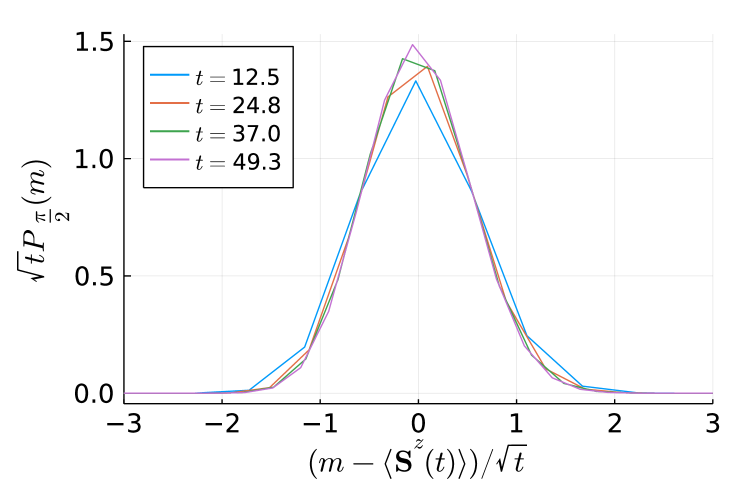
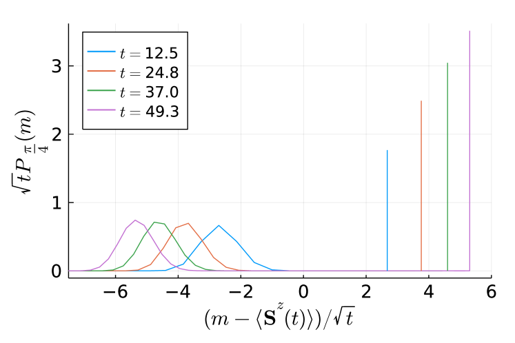
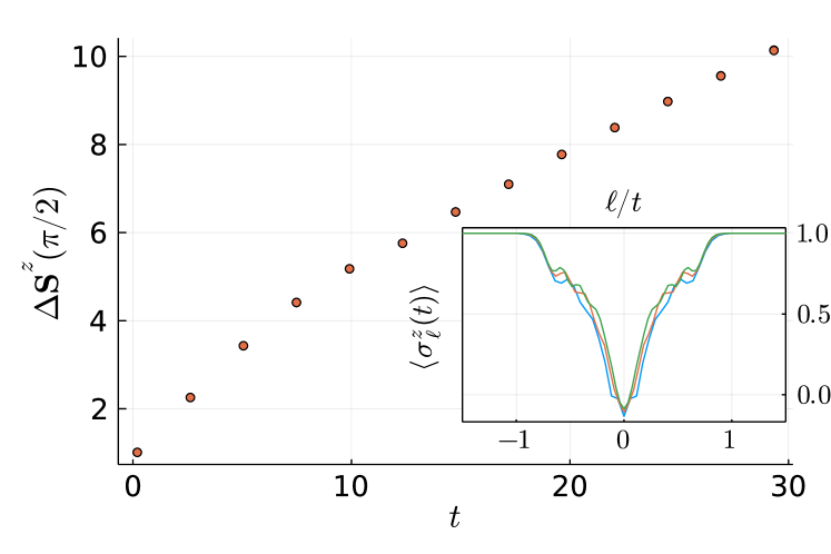
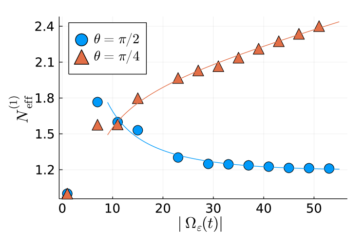
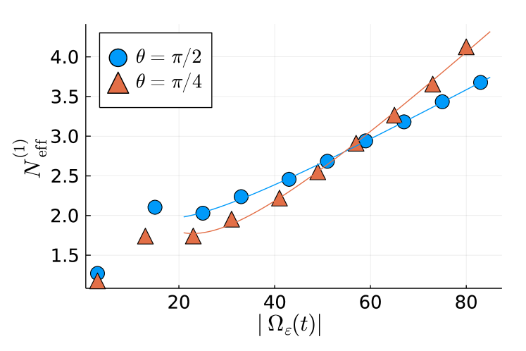
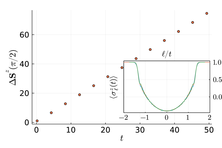
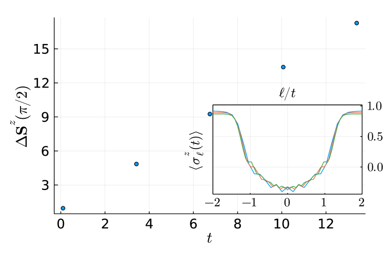
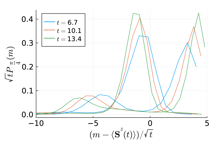
We measure macroscopic entanglement with the so called quantumness, which characterises the asymptotic behaviour of the maximum quantum Fisher information among all extensive observables (see Materials and Methods). In fact, we only compute a lower bound of it, 𝒩eff(1)superscriptsubscript𝒩eff1\mathcal{N}_{\mathrm{eff}}^{(1)}, resulting from reducing the space of observables. An example is reported in Fig. 3, where we plot 𝒩eff(1)superscriptsubscript𝒩eff1\mathcal{N}_{\mathrm{eff}}^{(1)} as a function of the effective system size |Ωϵ(t)|subscriptΩitalic-ϵ𝑡|\Omega_{\epsilon}(t)|. To study the asymptotic behavior of 𝒩eff(1)superscriptsubscript𝒩eff1\mathcal{N}_{\mathrm{eff}}^{(1)} we fit the data with a curve parametrised as β0+β1|Ωϵ(t)|+β21|Ωϵ(t)|subscript𝛽0subscript𝛽1subscriptΩitalic-ϵ𝑡subscript𝛽21subscriptΩitalic-ϵ𝑡\beta_{0}+\beta_{1}|\Omega_{\epsilon}(t)|+\beta_{2}\frac{1}{|\Omega_{\epsilon}(t)|}, where the term 1|Ωϵ(t)|1subscriptΩitalic-ϵ𝑡\frac{1}{|\Omega_{\epsilon}(t)|} stands for a potential sub-leading term. The estimated leading order is consistent with a constant (β10subscript𝛽10\beta_{1}\approx 0) in the case θ=π/2𝜃𝜋2\theta=\pi/2 and with a linear growth (β10subscript𝛽10\beta_{1}\neq 0) in the generic case. The figure also shows how the difference of magnetization between flipping or not the spin is proportional to |Ωϵ(t)|subscriptΩitalic-ϵ𝑡|\Omega_{\epsilon}(t)|, meaning that the two states |ket\ket{\Uparrow} and |Ψπ/2(t)ketsubscriptΨ𝜋2𝑡\ket{\Psi_{\pi/2}(t)} are macroscopically different and therefore the state |Ψθ(t)ketsubscriptΨ𝜃𝑡\ket{\Psi_{\theta}(t)} is macroscopically entangled for generic θ𝜃\theta. Fig. 3 also reports the probability density Pθ(m)subscript𝑃𝜃𝑚P_{\theta}(m) to get m𝑚m from a measurement of 𝐒zsuperscript𝐒𝑧\boldsymbol{\mathbf{S}}^{z} given that the system is in the state |Ψθ(t)ketsubscriptΨ𝜃𝑡\ket{\Psi_{\theta}(t)}; the case θ=π2𝜃𝜋2\theta=\frac{\pi}{2} shows standard fluctuations, while the more general case θ=π4𝜃𝜋4\theta=\frac{\pi}{4} shows the bimodal distribution that is characteristic of a cat state. We have shifted m𝑚m by the expectation value of 𝐒z(t)superscript𝐒𝑧𝑡\boldsymbol{\mathbf{S}}^{z}(t) so as to exhibit plots that are independent of the system’s size (incidentally, this also makes it equivalent to consider either the full chain or Ωϵ(t)subscriptΩitalic-ϵ𝑡\Omega_{\epsilon}(t)). The probability distribution in the GHZ state (|+|)/2ketket2(\ket{\Uparrow}+\ket{\Downarrow})/\sqrt{2} would exhibit two Kronecker deltas at the maximum and minimum magnetisations; here one delta is replaced by a Gaussian centred at a different magnetization, but it is still well separated from the other peak.
Refer to caption
Refer to caption
Refer to caption
Refer to caption
Figure 3: Time evolution of |Ψθ(t)ketsubscriptΨ𝜃𝑡\ket{\Psi_{\theta}(t)} under Hamiltonian 𝐇1subscript𝐇1\boldsymbol{\mathbf{H}}_{1} with J=2.8𝐽2.8J=2.8, γ=1𝛾1\gamma=1, w=Δ=Dz=hz=0𝑤Δsuperscript𝐷𝑧superscript𝑧0w=\Delta=D^{z}=h^{z}=0. From the top we have: 1) Difference between the total magnetization in |ket\ket{\Uparrow} and |Ψπ/2(t)ketsubscriptΨ𝜋2𝑡\ket{\Psi_{\pi/2}(t)}, i.e. Δ𝐒z(θ)=|𝐒z|Ψθ(t)|𝐒z|Ψθ(t)Δsuperscript𝐒𝑧𝜃quantum-operator-productsuperscript𝐒𝑧quantum-operator-productsubscriptΨ𝜃𝑡superscript𝐒𝑧subscriptΨ𝜃𝑡\Delta\boldsymbol{\mathbf{S}}^{z}(\theta)=\braket{\Uparrow}{\boldsymbol{\mathbf{S}}^{z}}{\Uparrow}-\braket{\Psi_{\theta}(t)}{\boldsymbol{\mathbf{S}}^{z}}{\Psi_{\theta}(t)}; inset: local magnetization profile for the last four times of the main plot. 2) Macroscopic quantumness Neff(1)superscriptsubscript𝑁eff1N_{\mathrm{eff}}^{(1)} as a function of the effective system size |Ωϵ(t)|subscriptΩitalic-ϵ𝑡|\Omega_{\epsilon}(t)|, with ϵ=0.001italic-ϵ0.001\epsilon=0.001. 3) and 4) Probability density Pθ(m)subscript𝑃𝜃𝑚P_{\theta}(m) for θ=π2𝜃𝜋2\theta=\tfrac{\pi}{2} and θ=π4𝜃𝜋4\theta=\tfrac{\pi}{4} respectively.

We have checked that, as long as the initial state is in the bulk of the spectrum, the qualitative behaviour remains the same even moving away from integrability. An example is reported in Fig. 4. Remarkably, even in this non-integrable case the profiles of local magnetization (the insets in the plots of the total magnetization) computed at different times collapse to the same curve in the ray coordinate /t𝑡\ell/t, which manifests the ballistic change in the total magnetization. Note also that from the profile of the local magnetization we get a visual definition of Ωϵ(t)subscriptΩitalic-ϵ𝑡\Omega_{\epsilon}(t): it essentially coincides with the region with σz(t)1expectationsubscriptsuperscript𝜎𝑧𝑡1\braket{\sigma^{z}_{\ell}(t)}\not\approx 1.

Refer to caption
Refer to caption
Figure 4: The same as in the top plots of Fig. 3 for Hamiltonian 𝐇1subscript𝐇1\boldsymbol{\mathbf{H}}_{1} with J=1,γ=0.5,w=0.7,Δ=0,Dz=0.6,hz=0formulae-sequence𝐽1formulae-sequence𝛾0.5formulae-sequence𝑤0.7formulae-sequenceΔ0formulae-sequencesuperscript𝐷𝑧0.6superscript𝑧0J=1,\gamma=0.5,w=0.7,\Delta=0,D^{z}=0.6,h^{z}=0.

We mention that the tidy structure of the transistor Hamiltonian 𝐇1subscript𝐇1\boldsymbol{\mathbf{H}}_{1} allows for an alternative interpretation of the protocol. The state before the measurement has all transistor’s switches open, and time evolution is blocked. The measurement has the effect of turning a switch in a quantum superposition of open and closed (the switch is exactly closed only for θ=π2𝜃𝜋2\theta=\frac{\pi}{2}). Closing a switch enables Heisenberg and Dzyaloshinskii-Moriya interactions between the neighboring spins of the opposite leg of the chain, which, in turn, partially close other switches, and so on and so forth, leading to a complete reconfiguration of the state that affects a region whose size grows linearly in time.

2.4 Generic model

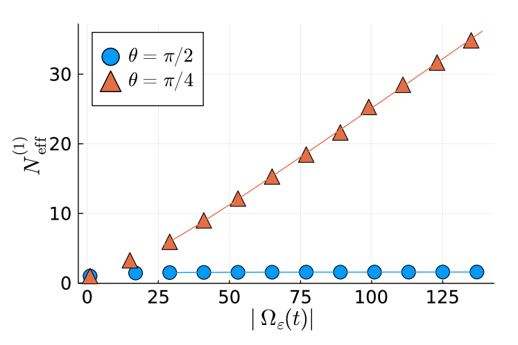
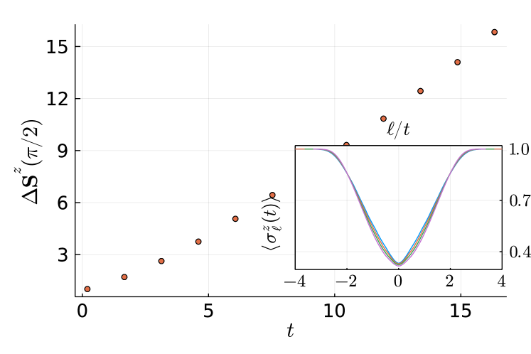
We have considered several models without a hidden U(1)𝑈1U(1) symmetry in which |ket\ket{\Uparrow} is still a quantum scar. We see quite generally that, also in those cases, the spin flip has everlasting effects arbitrarily far from the origin. In Fig. 5 we report an example using the Hamiltonian 𝐇2subscript𝐇2\boldsymbol{\mathbf{H}}_{2}. The plot of the magnetization shows that the states |ket\ket{\Uparrow} and |Ψπ/2(t)ketsubscriptΨ𝜋2𝑡\ket{\Psi_{\pi/2}(t)} are macroscopically different, indeed the difference of the magnetization in the two states grows linearly with the effective system size. Again, we conclude that our protocol leads to the formation of a macroscopically entangled state. Concerning the quantumness, we have fitted the data for the lower bound 𝒩eff(1)superscriptsubscript𝒩eff1\mathcal{N}_{\mathrm{eff}}^{(1)} with the same Ansatz as before β0+β1|Ωϵ(t)|+β21|Ωϵ(t)|subscript𝛽0subscript𝛽1subscriptΩitalic-ϵ𝑡subscript𝛽21subscriptΩitalic-ϵ𝑡\beta_{0}+\beta_{1}|\Omega_{\epsilon}(t)|+\beta_{2}\frac{1}{|\Omega_{\epsilon}(t)|}; the analysis points to an asymptotic linear growth for any θ0𝜃0\theta\neq 0, including this time also θ=π2𝜃𝜋2\theta=\frac{\pi}{2}. Therefore, |Ψθ(t)ketsubscriptΨ𝜃𝑡\ket{\Psi_{\theta}(t)} still exhibits macroscopic entanglement for generic θ𝜃\theta, but, in contrast to the quantum transistor chain, also |Ψπ/2(t)ketsubscriptΨ𝜋2𝑡\ket{\Psi_{\pi/2}(t)} is macroscopically entangled, undermining in turn the formation of a cat state.
Refer to caption
Refer to caption
Figure 5: The same as in the top plots of Fig. 3 for Hamiltonian 𝐇2subscript𝐇2\boldsymbol{\mathbf{H}}_{2} with J1=J2=1subscript𝐽1subscript𝐽21J_{1}=J_{2}=1, Jr>2=0subscript𝐽𝑟20J_{r>2}=0, γ1z=γ2z=0.6subscriptsuperscript𝛾𝑧1subscriptsuperscript𝛾𝑧20.6\gamma^{z}_{1}=\gamma^{z}_{2}=-0.6, Dr>1y=hz=γr>2z=0superscriptsubscript𝐷𝑟1𝑦superscript𝑧subscriptsuperscript𝛾𝑧𝑟20D_{r>1}^{y}=h^{z}=\gamma^{z}_{r>2}=0, D1y=0.9superscriptsubscript𝐷1𝑦0.9D_{1}^{y}=-0.9, γrx=γry=Drx=Drz=0,rformulae-sequencesubscriptsuperscript𝛾𝑥𝑟subscriptsuperscript𝛾𝑦𝑟subscriptsuperscript𝐷𝑥𝑟subscriptsuperscript𝐷𝑧𝑟0for-all𝑟\gamma^{x}_{r}=\gamma^{y}_{r}=D^{x}_{r}=D^{z}_{r}=0,\forall r. The widest profile in the inset corresponds to the largest time.

2.5 Imperfections in the preparation of the state

We investigate the effect of perturbing the state by time evolution under a homogeneous Hamiltonian 𝐇0subscript𝐇0\boldsymbol{\mathbf{H}}_{0} for a fixed time t0subscript𝑡0t_{0}, i.e., |Ψ0(0)=ei𝐇0t0|ketsubscriptΨ0superscript0superscript𝑒𝑖subscript𝐇0subscript𝑡0ket\ket{\Psi_{0}(0^{-})}=e^{-i\boldsymbol{\mathbf{H}}_{0}t_{0}}\ket{\Uparrow}. We then study the time evolution of |Ψθ(0+)=eiθ𝝈0y|Ψ0(0)ketsubscriptΨ𝜃superscript0superscript𝑒𝑖𝜃superscriptsubscript𝝈0𝑦ketsubscriptΨ0superscript0\ket{\Psi_{\theta}(0^{+})}=e^{i\theta\boldsymbol{\mathbf{\sigma}}_{0}^{y}}\ket{\Psi_{0}(0^{-})}, which is the analog of Eq. [2]. We warn the reader of a complication: the initial evolution affects the whole chain, so, strictly speaking, there is no approximately pure subsystem. If we insist on considering the subsystem associated with the spreading of the local perturbation (corresponding to the sharp change of behaviour in the profile of the magnetization), we should analyse the quantum Fisher information of a mixed state, which is a harder quantity to compute. In this preliminary study of the stability of our protocol, we limit ourselves to check the qualitative behaviour of the probability distribution of the magnetization.

We distinguish two classes of perturbations: in the first class, the perturbation is spin-flip symmetric (thus the hidden U(1)𝑈1U(1) symmetry is preserved), e.g., 𝐇0subscript𝐇0\boldsymbol{\mathbf{H}}_{0} could be the integrable Ising Hamiltonian

𝐇0,1=14(𝝈x𝝈+1x+h0z𝝈z);subscript𝐇0114subscriptsuperscriptsubscript𝝈𝑥superscriptsubscript𝝈1𝑥superscriptsubscript0𝑧superscriptsubscript𝝈𝑧\boldsymbol{\mathbf{H}}_{0,1}=-\frac{1}{4}\sum_{\ell}\left(\boldsymbol{\mathbf{\sigma}}_{\ell}^{x}\boldsymbol{\mathbf{\sigma}}_{\ell+1}^{x}+h_{0}^{z}\boldsymbol{\mathbf{\sigma}}_{\ell}^{z}\right)\,; (11)

in the second class, the pre-measuerement Hamiltonian breaks the spin-flip invariance behind the hidden U(1)𝑈1U(1) symmetry, e.g.

𝐇0,2=14(𝝈x𝝈+1x+h0z𝝈z+h0x𝝈x),subscript𝐇0214subscriptsuperscriptsubscript𝝈𝑥superscriptsubscript𝝈1𝑥superscriptsubscript0𝑧superscriptsubscript𝝈𝑧superscriptsubscript0𝑥superscriptsubscript𝝈𝑥\boldsymbol{\mathbf{H}}_{0,2}=-\frac{1}{4}\sum_{\ell}\left(\boldsymbol{\mathbf{\sigma}}_{\ell}^{x}\boldsymbol{\mathbf{\sigma}}_{\ell+1}^{x}+h_{0}^{z}\boldsymbol{\mathbf{\sigma}}_{\ell}^{z}+h_{0}^{x}\boldsymbol{\mathbf{\sigma}}_{\ell}^{x}\right)\,, (12)

which is a non-integrable version of the Ising model. Note that, in both cases, the larger h0zsuperscriptsubscript0𝑧h_{0}^{z}, the smaller the expected effect, therefore h0zsuperscriptsubscript0𝑧h_{0}^{z} can be used as a control parameter.

The first class of perturbations is not expected to destabilize the growth of a cat state: On the one hand, Ref. [31] showed that the perturbation has everlasting macroscopic effects even after so-called “global quenches” from a spin-flip invariant initial state. On the other hand, Ref. [50] indirectly confirms clustering in |Ψπ/2(t)ketsubscriptΨ𝜋2𝑡\ket{\Psi_{\pi/2}(t)} at long times with noninteracting transistor Hamiltonians, indeed the mutual information approaches zero at large distances. Our numerical analysis is consistent with these expectations, indeed we still see the formation of a bimodal probability distribution (with two well separated peaks).

On the contrary, for the second class of perturbations the probability density does not present two well separated peaks, as shown e.g. in the bottom row of Fig. 6. This rules out the formation of a cat state, but the basic features pointing to macroscopic entanglement (such as the linear growth in time of the difference of magnetization between flipping or not the spin) are still present for times longer than our maximum simulation times.
Refer to caption
Refer to caption
Figure 6: Time evolution under 𝐇1subscript𝐇1\boldsymbol{\mathbf{H}}_{1} after perturbing the state |ket\ket{\Uparrow} with 𝐇0,2subscript𝐇02\boldsymbol{\mathbf{H}}_{0,2} for a time t0=0.4subscript𝑡00.4t_{0}=0.4. The parameters are set to J=2.8𝐽2.8J=2.8, γ=1𝛾1\gamma=1, w=Δ=Dz=hz=0𝑤Δsuperscript𝐷𝑧superscript𝑧0w=\Delta=D^{z}=h^{z}=0, for 𝐇1subscript𝐇1\boldsymbol{\mathbf{H}}_{1}, and h0z=0.7subscriptsuperscript𝑧00.7h^{z}_{0}=0.7 and h0x=0.5subscriptsuperscript𝑥00.5h^{x}_{0}=0.5 for 𝐇0,2subscript𝐇02\boldsymbol{\mathbf{H}}_{0,2}. Top: the difference in magnetization with or without the spin flip grows linearly in time, at least for the times reached by our simulation. Bottom: more than two peaks appear and they are not well separated.

3 Discussion

3.1 Local perturbations with macroscopic effects

In ordinary 1D systems a spin flip does not change the macroscopic properties of a state whatever long the time is. The naive expectation is that its effect spreads out across the chain as tαsuperscript𝑡𝛼t^{\alpha} but fades away as tαsuperscript𝑡𝛼t^{-\alpha}, with α=1𝛼1\alpha=1 in integrable models and α=12𝛼12\alpha=\tfrac{1}{2} in most of the generic systems. Recently, three situations have been pointed out in which this picture can break down:

  • ground states in symmetry-broken phases [51, 52].

  • quantum jammed states in systems with Hilbert space fragmentation [41].

  • systems with semilocal conservation laws [31].

To these three known cases, we have added models with a fully separable quantum scar. This novel scenario has two advantages: first, a product state can be easily prepared experimentally, and, second, its stationarity gives the freedom to stop the (virtual) experiment at any time without compromising the outcome.

Remarkably, the norm is that the perturbation generates macroscopic entanglement, indeed, the possible but improbable operators breaking that rule can be cured by the addition of a local operator that does not change the excited state — e.g., ϵ𝝈zitalic-ϵsuperscriptsubscript𝝈𝑧\epsilon\boldsymbol{\mathbf{\sigma}}_{\ell}^{z} for our initial state |ket\ket{\Uparrow}.

In the special case in which there is a hidden U(1)𝑈1U(1) symmetry our analysis of the fluctuations reveals that the entangled part of the system is in a Schrödinger’s cat state.

3.2 On the spreading

The existence of the semilocal charge 𝚷z()subscriptsuperscript𝚷𝑧\sum_{\ell}\boldsymbol{\mathbf{\Pi}}^{z}(\ell) ensures that the effect of the spin flip does not fade away at long time [31, 32], but it is not sufficient to exclude the effect to remain confined around the position of the measurement. This is indeed what happens when hh is too large, in which case the Hamiltonian exhibits localised excitations (see Appendix B). In the generic case, however, the perturbation spreads out. Using the underlying integrable structure, Ref. [31] showed that the spreading is ballistic for γ=1𝛾1\gamma=1, w=Δ=Dz=0𝑤Δsuperscript𝐷𝑧0w=\Delta=D^{z}=0, and |hz|<14superscript𝑧14|h^{z}|<\frac{1}{4}. And for slightly different initial product states, ballistic behaviour was observed [41, 42] also for γ=w=Δ=Dz=hz=0𝛾𝑤Δsuperscript𝐷𝑧superscript𝑧0\gamma=w=\Delta=D^{z}=h^{z}=0, for which the model is integrable as well. A priori one would not expect ballistic spreading in generic models, but rather diffusive. In Ref. [41], in particular, a preliminary analysis of the effect of some integrability-breaking perturbations pointed to a non-ballistic spreading. In contrast, we find numerical evidence that ballistic behaviour extends to a wide range of parameters, at least, within the time window investigated. In order to rule integrability out, we have checked the statistics of the energy levels, and, for generic parameters, our data are in excellent agreement with a Wigner-Dyson distribution (see the Appendix A), supporting, in turn, the non-integrability of the generic models investigated.

4 Materials and Methods

4.1 Simulations of the dynamics

Numerical simulations are performed with Julia ITensor library [53]. We use a time-evolving block decimation (TEBD) algorithm and, in all data reported, time evolution is discretized in time steps δt=0.01𝛿𝑡0.01\delta t=0.01 with 2nd order Trotter-Suzuki gates [54].

4.2 Full counting statistics

The full probability distribution of a given observable encodes the entire information about its moments. Let L𝐿L be the chain’s length. We define Pθ(m)subscript𝑃𝜃𝑚P_{\theta}(m) as the probability to get m𝑚m from a measurement of 𝐒zsuperscript𝐒𝑧\boldsymbol{\mathbf{S}}^{z} given that the system is in the state |Ψθ(t)ketsubscriptΨ𝜃𝑡\ket{\Psi_{\theta}(t)}. Note that m{L2,L2+1,,L2}𝑚𝐿2𝐿21𝐿2m\in\{-\frac{L}{2},-\frac{L}{2}+1,...,\frac{L}{2}\}. To set a convention, we assume L𝐿L to be divisible by 444, so that the maximum possible value m𝑚m of the magnetization is an integer even number. The generating function of the moments of the probability distribution is defined as

Gθ(k)=Ψθ(t)|ei2πkL+1𝐒z|Ψθ(t).subscript𝐺𝜃𝑘quantum-operator-productsubscriptΨ𝜃𝑡superscript𝑒𝑖2𝜋𝑘𝐿1superscript𝐒𝑧subscriptΨ𝜃𝑡G_{\theta}(k)=\braket{\Psi_{\theta}(t)}{e^{i\frac{2\pi k}{L+1}\boldsymbol{\mathbf{S}}^{z}}}{\Psi_{\theta}(t)}. (13)

The probability Pθ(m)subscript𝑃𝜃𝑚P_{\theta}(m) is then the Fourier transform of the generating function:

Pθ(m)=1L+1k=L/2L/2ei2πkL+1mGθ(k).subscript𝑃𝜃𝑚1𝐿1superscriptsubscript𝑘𝐿2𝐿2superscript𝑒𝑖2𝜋𝑘𝐿1𝑚subscript𝐺𝜃𝑘P_{\theta}(m)=\frac{1}{L+1}\sum_{k=-L/2}^{L/2}e^{-i\frac{2\pi k}{L+1}m}G_{\theta}(k). (14)

We compute the generating function numerically using Julia ITensor library [53].

We point out that, if the model is invariant under spin flip 𝝈x,y𝝈x,ysuperscript𝝈𝑥𝑦superscript𝝈𝑥𝑦\boldsymbol{\mathbf{\sigma}}^{x,y}\rightarrow-\boldsymbol{\mathbf{\sigma}}^{x,y}, the state |Ψπ/2(t)ketsubscriptΨ𝜋2𝑡\ket{\Psi_{\pi/2}(t)} belongs to the sector in which the parity operator 𝚷z=𝝈zsuperscript𝚷𝑧subscriptproductsubscriptsuperscript𝝈𝑧\boldsymbol{\mathbf{\Pi}}^{z}=\prod_{\ell}\boldsymbol{\mathbf{\sigma}}^{z}_{\ell} has eigenvalue 11-1, which means Pπ/2(m)=0subscript𝑃𝜋2𝑚0P_{\pi/2}(m)=0 for any even m𝑚m. This implies that, in the generic case of |Ψθ(t)ketsubscriptΨ𝜃𝑡\ket{\Psi_{\theta}(t)} with θπ2𝜃𝜋2\theta\neq\frac{\pi}{2}, Pθ(m)=0subscript𝑃𝜃𝑚0P_{\theta}(m)=0 for any even m𝑚m except for Pθ(L/2)=cos2θsubscript𝑃𝜃𝐿2superscript2𝜃P_{\theta}(L/2)=\cos^{2}\theta. This is why, in the plots of the probability density for models with spin-flip invariance, we report only odd values of m𝑚m and m=L/2𝑚𝐿2m=L/2.

4.3 Quantumness and Quantum Fisher information

Ref. [55] proposed the quantum Fisher information as a measure of the “macroscopicity” of quantum effects in lattice systems. Its computation is however rather complicated when addressed in full generality, both analytically and numerically. For the sake of simplicity, we follow the approach of Refs [56, 28, 29] and restrict ourselves to examining a sufficient condition. Specifically, we investigate the quantum Fisher information (𝐎)𝐎\mathcal{F}(\boldsymbol{\mathbf{O}}) of extensive operators whose densities have support on a single site, i.e., 𝐎[{n}]=jΩϵ(t)nj𝝈j𝐎delimited-[]𝑛subscript𝑗subscriptΩitalic-ϵ𝑡subscript𝑛𝑗subscript𝝈𝑗\boldsymbol{\mathbf{O}}[\{\vec{n}\}]=\sum_{j\in\Omega_{\epsilon}(t)}\vec{n}_{j}\cdot\vec{\boldsymbol{\mathbf{\sigma}}}_{j}, where 𝝈j{𝝈jx,𝝈jy,𝝈jz}subscript𝝈𝑗subscriptsuperscript𝝈𝑥𝑗subscriptsuperscript𝝈𝑦𝑗subscriptsuperscript𝝈𝑧𝑗\vec{\boldsymbol{\mathbf{\sigma}}}_{j}\equiv\{\boldsymbol{\mathbf{\sigma}}^{x}_{j},\boldsymbol{\mathbf{\sigma}}^{y}_{j},\boldsymbol{\mathbf{\sigma}}^{z}_{j}\} and the coefficients are normalised as |nj|2=1superscriptsubscript𝑛𝑗21|\vec{n}_{j}|^{2}=1. In pure states, which is the case we consider, (𝐎)𝐎\mathcal{F}(\boldsymbol{\mathbf{O}}) equals four times the variance of 𝐎𝐎\boldsymbol{\mathbf{O}}. Using the notation of [30], we introduce the quantumness Neffsubscript𝑁effN_{\mathrm{eff}} of a state as its maximal quantum Fisher information with respect to all extensive observables:

Neff=14|Ωϵ(t)|max𝐎(𝐎).subscript𝑁eff14subscriptΩitalic-ϵ𝑡subscript𝐎𝐎N_{\mathrm{eff}}=\frac{1}{4|\Omega_{\epsilon}(t)|}\max_{\boldsymbol{\mathbf{O}}}\mathcal{F}(\boldsymbol{\mathbf{O}}). (15)

We denote by Neff(1)superscriptsubscript𝑁eff1N_{\mathrm{eff}}^{(1)} the maximisation restricted to the observables with single-site density as introduced above. Neffsubscript𝑁effN_{\mathrm{eff}} was interpreted as an effective size of the macroscopic quantum state, thus Neff(1)superscriptsubscript𝑁eff1N_{\mathrm{eff}}^{(1)} is a lower bound for the effective size. We introduce the covariance matrix

[K(t)]n,α;m,β=12Ψπ/2(t)|{𝝈nα,𝝈mβ}|Ψπ/2(t)+Ψπ/2(t)|𝝈nα|Ψπ/2(t)Ψπ/2(t)|𝝈mβ|Ψπ/2(t),[\mathrm{K}(t)]_{n,\alpha;m,\beta}=\frac{1}{2}\braket{\Psi_{\pi/2}(t)}{\{\boldsymbol{\mathbf{\sigma}}_{n}^{\alpha},\boldsymbol{\mathbf{\sigma}}_{m}^{\beta}\}}{\Psi_{\pi/2}(t)}+\\ -\braket{\Psi_{\pi/2}(t)}{\boldsymbol{\mathbf{\sigma}}_{n}^{\alpha}}{\Psi_{\pi/2}(t)}\braket{\Psi_{\pi/2}(t)}{\boldsymbol{\mathbf{\sigma}}_{m}^{\beta}}{\Psi_{\pi/2}(t)}\,, (16)

where {𝝈nα,𝝈mβ}=𝝈nα𝝈mβ+𝝈mβ𝝈nαsuperscriptsubscript𝝈𝑛𝛼superscriptsubscript𝝈𝑚𝛽superscriptsubscript𝝈𝑛𝛼superscriptsubscript𝝈𝑚𝛽superscriptsubscript𝝈𝑚𝛽superscriptsubscript𝝈𝑛𝛼\{\boldsymbol{\mathbf{\sigma}}_{n}^{\alpha},\boldsymbol{\mathbf{\sigma}}_{m}^{\beta}\}=\boldsymbol{\mathbf{\sigma}}_{n}^{\alpha}\boldsymbol{\mathbf{\sigma}}_{m}^{\beta}+\boldsymbol{\mathbf{\sigma}}_{m}^{\beta}\boldsymbol{\mathbf{\sigma}}_{n}^{\alpha}. In pure states, 𝒩eff(1)superscriptsubscript𝒩eff1\mathcal{N}_{\mathrm{eff}}^{(1)} satisfies

𝒩eff(1)=tr[D(t)]|Ωϵ(t)|,withK(t)v(t)=[D(t)I3]v(t),formulae-sequencesuperscriptsubscript𝒩eff1trdelimited-[]D𝑡subscriptΩitalic-ϵ𝑡withK𝑡𝑣𝑡delimited-[]tensor-productD𝑡subscriptI3𝑣𝑡\mathcal{N}_{\mathrm{eff}}^{(1)}=\frac{\mathrm{tr}[\mathrm{D}(t)]}{|\Omega_{\epsilon}(t)|}\,,\quad\text{with}\quad\mathrm{K}(t)\vec{v}(t)=[\mathrm{D}(t)\otimes\mathrm{I}_{3}]\vec{v}(t)\,, (17)

where n,mΩϵ(t)𝑛𝑚subscriptΩitalic-ϵ𝑡n,m\in\Omega_{\epsilon}(t) (the vector space is 3|Ωϵ(t)|3subscriptΩitalic-ϵ𝑡3|\Omega_{\epsilon}(t)|-dimensional) and D(t)D𝑡\mathrm{D}(t) is required to be diagonal ([v]nsubscriptdelimited-[]𝑣𝑛[\vec{v}]_{n} are normalised). We solve Eq. [17] using a Lanczos algorithm with three basic iterative steps:

  1. 1.

    w(n)=Kv(n)superscript𝑤𝑛Ksuperscript𝑣𝑛\vec{w}^{(n)}=\mathrm{K}\vec{v}^{(n)}

  2. 2.

    [D(n)]j=wj(n)1subscriptdelimited-[]superscriptD𝑛𝑗superscriptnormsuperscriptsubscript𝑤𝑗𝑛1[\mathrm{D}^{(n)}]_{j}=\parallel\vec{w}_{j}^{(n)}\parallel^{-1}

  3. 3.

    v(n+1)=(D(n)I3)w(n)superscript𝑣𝑛1tensor-productsuperscriptD𝑛subscriptI3superscript𝑤𝑛\vec{v}^{(n+1)}=(\mathrm{D}^{(n)}\otimes\mathrm{I}_{3})\vec{w}^{(n)}

In most of the cases this procedure worked well without particular stabilizers.

5 Conclusion

We have shown that, quite generally, macroscopic entanglement emerges from a localised inhomogeneity in a state that would be otherwise stationary. This can not happen in an ordinary excited state that maximises the entropy under the constraints of the local conservation laws. In generic systems, indeed, we observe the phenomenon in quantum scars with anomalously low bipartite entanglement. We also argue that, in the specific case in which the excited state maximises instead the entropy under the constraints of also semi-local conservation laws, macroscopic entanglement takes the simple form of a cat state, providing in turn a novel way to generate cat states in a class of quantum many-body systems with local interactions.

This work leaves several open questions. First, a rigorous proof of the generation of cat states is missing. Second, the observation of ballistic behaviour in generic systems could be questioned as a finite-time effect, so additional investigations are imperative. Third, we have only provided a preliminary and incomplete check of the stability of our protocol, but this is clearly an important issue and does require additional investigations.

S.B. thanks Tommaso Roscilde and Augusto Smerzi for useful discussions. This work was supported by the European Research Council under the Starting Grant No. 805252 LoCoMacro.

References

  • Schrödinger [1935] E. Schrödinger. Die gegenwärtige Situation in der Quantenmechanik. Naturwissenschaften, 23(48):807–812, Nov 1935. ISSN 1432-1904. doi: 10.1007/BF01491891. URL https://doi.org/10.1007/BF01491891.
  • Trimmer [1980] John D. Trimmer. The Present Situation in Quantum Mechanics: A Translation of Schrödinger’s "Cat Paradox" Paper. Proceedings of the American Philosophical Society, 124(5):323–338, 1980. ISSN 0003049X. URL http://www.jstor.org/stable/986572.
  • Greenberger et al. [1989] Daniel M. Greenberger, Michael A. Horne, and Anton Zeilinger. Going Beyond Bell’s Theorem, pages 69–72. Springer Netherlands, Dordrecht, 1989. ISBN 978-94-017-0849-4. doi: 10.1007/978-94-017-0849-4_10. URL https://doi.org/10.1007/978-94-017-0849-4_10.
  • Bell [1964] J. S. Bell. On the Einstein Podolsky Rosen paradox. Physics Physique Fizika, 1:195–200, Nov 1964. doi: 10.1103/PhysicsPhysiqueFizika.1.195. URL https://link.aps.org/doi/10.1103/PhysicsPhysiqueFizika.1.195.
  • Agarwal et al. [1997] G. S. Agarwal, R. R. Puri, and R. P. Singh. Atomic schrödinger cat states. Phys. Rev. A, 56:2249–2254, Sep 1997. doi: 10.1103/PhysRevA.56.2249. URL https://link.aps.org/doi/10.1103/PhysRevA.56.2249.
  • Lombardo and Twamley [2015] Daniel Lombardo and Jason Twamley. Deterministic Creation of Macroscopic Cat States. Scientific Reports, 5(1):13884, Sep 2015. ISSN 2045-2322. doi: 10.1038/srep13884. URL https://doi.org/10.1038/srep13884.
  • Wang et al. [2016] Chen Wang, Yvonne Y. Gao, Philip Reinhold, R. W. Heeres, Nissim Ofek, Kevin Chou, Christopher Axline, Matthew Reagor, Jacob Blumoff, K. M. Sliwa, L. Frunzio, S. M. Girvin, Liang Jiang, M. Mirrahimi, M. H. Devoret, and R. J. Schoelkopf. A Schrödinger cat living in two boxes. Science, 352(6289):1087–1091, 2016. doi: 10.1126/science.aaf2941. URL https://www.science.org/doi/abs/10.1126/science.aaf2941.
  • Hacker et al. [2019] Bastian Hacker, Stephan Welte, Severin Daiss, Armin Shaukat, Stephan Ritter, Lin Li, and Gerhard Rempe. Deterministic creation of entangled atom–light Schrödinger-cat states. Nature Photonics, 13(2):110–115, Feb 2019. ISSN 1749-4893. doi: 10.1038/s41566-018-0339-5. URL https://doi.org/10.1038/s41566-018-0339-5.
  • Alexander et al. [2020] Byron Alexander, John J. Bollinger, and Hermann Uys. Generating Greenberger-Horne-Zeilinger states with squeezing and postselection. Phys. Rev. A, 101:062303, Jun 2020. doi: 10.1103/PhysRevA.101.062303. URL https://link.aps.org/doi/10.1103/PhysRevA.101.062303.
  • Zhao et al. [2021] Yajuan Zhao, Rui Zhang, Wenlan Chen, Xiang-Bin Wang, and Jiazhong Hu. Creation of Greenberger-Horne-Zeilinger states with thousands of atoms by entanglement amplification. npj Quantum Information, 7(1):24, Feb 2021. ISSN 2056-6387. doi: 10.1038/s41534-021-00364-8. URL https://doi.org/10.1038/s41534-021-00364-8.
  • Cosacchi et al. [2021] M. Cosacchi, T. Seidelmann, J. Wiercinski, M. Cygorek, A. Vagov, D. E. Reiter, and V. M. Axt. Schrödinger cat states in quantum-dot-cavity systems. Phys. Rev. Research, 3:023088, May 2021. doi: 10.1103/PhysRevResearch.3.023088. URL https://link.aps.org/doi/10.1103/PhysRevResearch.3.023088.
  • Wang et al. [2022] Zhiling Wang, Zenghui Bao, Yukai Wu, Yan Li, Weizhou Cai, Weiting Wang, Yuwei Ma, Tianqi Cai, Xiyue Han, Jiahui Wang, Yipu Song, Luyan Sun, Hongyi Zhang, and Luming Duan. A flying Schrödinger’s cat in multipartite entangled states. Science Advances, 8(10):eabn1778, 2022. doi: 10.1126/sciadv.abn1778. URL https://www.science.org/doi/abs/10.1126/sciadv.abn1778.
  • Comparin et al. [2022] Tommaso Comparin, Fabio Mezzacapo, and Tommaso Roscilde. Multipartite entangled states in dipolar quantum simulators. Phys. Rev. Lett., 129:150503, Oct 2022. doi: 10.1103/PhysRevLett.129.150503. URL https://link.aps.org/doi/10.1103/PhysRevLett.129.150503.
  • Gao et al. [2010] Wei-Bo Gao, Chao-Yang Lu, Xing-Can Yao, Ping Xu, Otfried Gühne, Alexander Goebel, Yu-Ao Chen, Cheng-Zhi Peng, Zeng-Bing Chen, and Jian-Wei Pan. Experimental demonstration of a hyper-entangled ten-qubit Schrödinger cat state. Nature Physics, 6(5):331–335, May 2010. ISSN 1745-2481. doi: 10.1038/nphys1603. URL https://doi.org/10.1038/nphys1603.
  • Etesse et al. [2015] Jean Etesse, Martin Bouillard, Bhaskar Kanseri, and Rosa Tualle-Brouri. Experimental generation of squeezed cat states with an operation allowing iterative growth. Phys. Rev. Lett., 114:193602, May 2015. doi: 10.1103/PhysRevLett.114.193602. URL https://link.aps.org/doi/10.1103/PhysRevLett.114.193602.
  • Omran et al. [2019] A. Omran, H. Levine, A. Keesling, G. Semeghini, T. T. Wang, S. Ebadi, H. Bernien, A. S. Zibrov, H. Pichler, S. Choi, J. Cui, M. Rossignolo, P. Rembold, S. Montangero, T. Calarco, M. Endres, M. Greiner, V. Vuletic, and M. D. Lukin. Generation and manipulation of Schrödinger cat states in Rydberg atom arrays. Science, 365:570–574, 8 2019. doi: 10.1126/science.aax9743.
  • Song et al. [2019] Chao Song, Kai Xu, Hekang Li, Yu-Ran Zhang, Wuxin Liu, Qiujiang Guo, Zhen Wang, Wenhui Ren, Jie Hao, Hui Feng, Heng Fan, Dongning Zheng, Da-Wei Wang, H. Wang, and Shi-Yao Zhu. Generation of multicomponent atomic Schrödinger cat states of up to 20 qubits. Science, 365:574–577, 2019. doi: 10.1126/science.aay0600.
  • Shimizu and Miyadera [2002] Akira Shimizu and Takayuki Miyadera. Stability of quantum states of finite macroscopic systems against classical noises, perturbations from environments, and local measurements. Phys. Rev. Lett., 89:270403, Dec 2002. doi: 10.1103/PhysRevLett.89.270403. URL https://link.aps.org/doi/10.1103/PhysRevLett.89.270403.
  • Bernien et al. [2017] Hannes Bernien, Sylvain Schwartz, Alexander Keesling, Harry Levine, Ahmed Omran, Hannes Pichler, Soonwon Choi, Alexander S. Zibrov, Manuel Endres, Markus Greiner, Vladan Vuletić, and Mikhail D. Lukin. Probing many-body dynamics on a 51-atom quantum simulator. Nature, 551(7682):579–584, Nov 2017. ISSN 1476-4687. doi: 10.1038/nature24622. URL https://doi.org/10.1038/nature24622.
  • Turner et al. [2018] C. J. Turner, A. A. Michailidis, D. A. Abanin, M. Serbyn, and Z. Papić. Weak ergodicity breaking from quantum many-body scars. Nature Physics, 14(7):745–749, Jul 2018. ISSN 1745-2481. doi: 10.1038/s41567-018-0137-5. URL https://doi.org/10.1038/s41567-018-0137-5.
  • Moudgalya et al. [2022a] Sanjay Moudgalya, B Andrei Bernevig, and Nicolas Regnault. Quantum many-body scars and hilbert space fragmentation: a review of exact results. Reports on Progress in Physics, 85(8):086501, 7 2022a. doi: 10.1088/1361-6633/ac73a0. URL https://doi.org/10.1088/1361-6633/ac73a0.
  • Moudgalya et al. [2022b] Sanjay Moudgalya, B Andrei Bernevig, and Nicolas Regnault. Quantum many-body scars and hilbert space fragmentation: a review of exact results. Reports on Progress in Physics, 85(8):086501, jul 2022b. doi: 10.1088/1361-6633/ac73a0. URL https://doi.org/10.1088/1361-6633/ac73a0.
  • Dooley [2021] Shane Dooley. Robust quantum sensing in strongly interacting systems with many-body scars. PRX Quantum, 2:020330, May 2021. doi: 10.1103/PRXQuantum.2.020330. URL https://link.aps.org/doi/10.1103/PRXQuantum.2.020330.
  • Zhang et al. [2022] Pengfei Zhang, Hang Dong, Yu Gao, Liangtian Zhao, Jie Hao, Jean-Yves Desaules, Qiujiang Guo, Jiachen Chen, Jinfeng Deng, Bobo Liu, Wenhui Ren, Yunyan Yao, Xu Zhang, Shibo Xu, Ke Wang, Feitong Jin, Xuhao Zhu, Bing Zhang, Hekang Li, Chao Song, Zhen Wang, Fangli Liu, Zlatko Papić, Lei Ying, H. Wang, and Ying-Cheng Lai. Many-body Hilbert space scarring on a superconducting processor. Nature Physics, 18, 10 2022. ISSN 1745-2481. doi: 10.1038/s41567-022-01784-9. URL https://doi.org/10.1038/s41567-022-01784-9.
  • Desaules et al. [2022] Jean-Yves Desaules, Francesca Pietracaprina, Zlatko Papić, John Goold, and Silvia Pappalardi. Extensive multipartite entanglement from su(2) quantum many-body scars. Phys. Rev. Lett., 129:020601, Jul 2022. doi: 10.1103/PhysRevLett.129.020601. URL https://link.aps.org/doi/10.1103/PhysRevLett.129.020601.
  • Lieb and Robinson [1972] Elliot H. Lieb and Derek W. Robinson. The finite group velocity of quantum spin systems. Commun. Math. Phys., 28:251, 1972. doi: 10.1007/BF01645779. URL https://doi.org/10.1007/BF01645779.
  • Morimae et al. [2005] Tomoyuki Morimae, Ayumu Sugita, and Akira Shimizu. Macroscopic entanglement of many-magnon states. Physical Review A, 71(3), mar 2005. doi: 10.1103/physreva.71.032317. URL https://doi.org/10.1103%2Fphysreva.71.032317.
  • Hyllus et al. [2012] Philipp Hyllus, Wiesław Laskowski, Roland Krischek, Christian Schwemmer, Witlef Wieczorek, Harald Weinfurter, Luca Pezzé, and Augusto Smerzi. Fisher information and multiparticle entanglement. Phys. Rev. A, 85:022321, Feb 2012. doi: 10.1103/PhysRevA.85.022321. URL https://link.aps.org/doi/10.1103/PhysRevA.85.022321.
  • Tóth [2012] Géza Tóth. Multipartite entanglement and high-precision metrology. Phys. Rev. A, 85:022322, 2 2012. doi: 10.1103/PhysRevA.85.022322. URL https://link.aps.org/doi/10.1103/PhysRevA.85.022322.
  • Fröwis et al. [2018] Florian Fröwis, Pavel Sekatski, Wolfgang Dür, Nicolas Gisin, and Nicolas Sangouard. Macroscopic quantum states: Measures, fragility, and implementations. Rev. Mod. Phys., 90:025004, May 2018. doi: 10.1103/RevModPhys.90.025004. URL https://link.aps.org/doi/10.1103/RevModPhys.90.025004.
  • Fagotti [2022] Maurizio Fagotti. Global quenches after localized perturbations. Phys. Rev. Lett., 128:110602, Mar 2022. doi: 10.1103/PhysRevLett.128.110602. URL https://link.aps.org/doi/10.1103/PhysRevLett.128.110602.
  • Fagotti et al. [2022] Maurizio Fagotti, Vanja Marić, and Lenart Zadnik. Nonequilibrium symmetry-protected topological order: emergence of semilocal Gibbs ensembles. https://doi.org/10.48550/arXiv.2205.02221, 2022.
  • den Nijs and Rommelse [1989] Marcel den Nijs and Koos Rommelse. Preroughening transitions in crystal surfaces and valence-bond phases in quantum spin chains. Phys. Rev. B, 40:4709–4734, Sep 1989. doi: 10.1103/PhysRevB.40.4709. URL https://link.aps.org/doi/10.1103/PhysRevB.40.4709.
  • Pérez-García et al. [2008] D. Pérez-García, M. M. Wolf, M. Sanz, F. Verstraete, and J. I. Cirac. String Order and Symmetries in Quantum Spin Lattices. Phys. Rev. Lett., 100:167202, Apr 2008. doi: 10.1103/PhysRevLett.100.167202. URL https://link.aps.org/doi/10.1103/PhysRevLett.100.167202.
  • Endres et al. [2011] M. Endres, M. Cheneau, T. Fukuhara, C. Weitenberg, P. Schauß, C. Gross, L. Mazza, M. C. Bañuls, L. Pollet, I. Bloch, and S. Kuhr. Observation of Correlated Particle-Hole Pairs and String Order in Low-Dimensional Mott Insulators. Science, 334(6053):200–203, 2011. doi: 10.1126/science.1209284. URL https://www.science.org/doi/abs/10.1126/science.1209284.
  • Ilievski et al. [2016] Enej Ilievski, Marko Medenjak, Tomaž Prosen, and Lenart Zadnik. Quasilocal charges in integrable lattice systems. Journal of Statistical Mechanics: Theory and Experiment, 2016(6):064008, jun 2016. doi: 10.1088/1742-5468/2016/06/064008. URL https://doi.org/10.1088/1742-5468/2016/06/064008.
  • Zadnik and Fagotti [2021] Lenart Zadnik and Maurizio Fagotti. The Folded Spin-1/2 XXZ Model: I. Diagonalisation, Jamming, and Ground State Properties. SciPost Phys. Core, 4:10, 2021. doi: 10.21468/SciPostPhysCore.4.2.010. URL https://scipost.org/10.21468/SciPostPhysCore.4.2.010.
  • Pozsgay et al. [2021] Balázs Pozsgay, Tamás Gombor, and Arthur Hutsalyuk. Integrable hard-rod deformation of the heisenberg spin chains. Phys. Rev. E, 104:064124, Dec 2021. doi: 10.1103/PhysRevE.104.064124. URL https://link.aps.org/doi/10.1103/PhysRevE.104.064124.
  • Bariev [1991] R Z Bariev. Integrable spin chain with two- and three-particle interactions. Journal of Physics A: Mathematical and General, 24(10):L549–L553, may 1991. doi: 10.1088/0305-4470/24/10/010. URL https://doi.org/10.1088/0305-4470/24/10/010.
  • Zadnik et al. [2021a] Lenart Zadnik, Kemal Bidzhiev, and Maurizio Fagotti. The Folded Spin-1/2 XXZ Model: II. Thermodynamics and Hydrodynamics with a Minimal Set of Charges. SciPost Phys., 10:99, 2021a. doi: 10.21468/SciPostPhys.10.5.099. URL https://scipost.org/10.21468/SciPostPhys.10.5.099.
  • Bidzhiev et al. [2022] Kemal Bidzhiev, Maurizio Fagotti, and Lenart Zadnik. Macroscopic Effects of Localized Measurements in Jammed States of Quantum Spin Chains. Phys. Rev. Lett., 128:130603, Mar 2022. doi: 10.1103/PhysRevLett.128.130603. URL https://link.aps.org/doi/10.1103/PhysRevLett.128.130603.
  • Zadnik et al. [2021b] Lenart Zadnik, Saverio Bocini, Kemal Bidzhiev, and Maurizio Fagotti. Measurement catastrophe and ballistic spread of charge density with vanishing current. https://arxiv.org/abs/2111.06325, 2021b. URL https://arxiv.org/abs/2111.06325.
  • Monroe et al. [2021] C. Monroe, W. C. Campbell, L.-M. Duan, Z.-X. Gong, A. V. Gorshkov, P. W. Hess, R. Islam, K. Kim, N. M. Linke, G. Pagano, P. Richerme, C. Senko, and N. Y. Yao. Programmable quantum simulations of spin systems with trapped ions. Rev. Mod. Phys., 93:025001, Apr 2021. doi: 10.1103/RevModPhys.93.025001. URL https://link.aps.org/doi/10.1103/RevModPhys.93.025001.
  • Mikeska and Kolezhuk [2004] Hans-Jürgen Mikeska and Alexei K. Kolezhuk. One-dimensional magnetism, pages 1–83. Springer Berlin Heidelberg, Berlin, Heidelberg, 2004. ISBN 978-3-540-40066-0. doi: 10.1007/BFb0119591. URL https://doi.org/10.1007/BFb0119591.
  • Müller and Shrock [1985] Gerhard Müller and Robert E. Shrock. Implications of direct-product ground states in the one-dimensional quantum XYZ and XY spin chains. Phys. Rev. B, 32:5845–5850, Nov 1985. doi: 10.1103/PhysRevB.32.5845. URL https://link.aps.org/doi/10.1103/PhysRevB.32.5845.
  • van Horssen et al. [2015] Merlijn van Horssen, Emanuele Levi, and Juan P. Garrahan. Dynamics of many-body localization in a translation-invariant quantum glass model. Phys. Rev. B, 92:100305, Sep 2015. doi: 10.1103/PhysRevB.92.100305. URL https://link.aps.org/doi/10.1103/PhysRevB.92.100305.
  • Pancotti et al. [2020] Nicola Pancotti, Giacomo Giudice, J. Ignacio Cirac, Juan P. Garrahan, and Mari Carmen Bañuls. Quantum east model: Localization, nonthermal eigenstates, and slow dynamics. Phys. Rev. X, 10:021051, Jun 2020. doi: 10.1103/PhysRevX.10.021051. URL https://link.aps.org/doi/10.1103/PhysRevX.10.021051.
  • Bravyi et al. [2006] S. Bravyi, M. B. Hastings, and F. Verstraete. Lieb-robinson bounds and the generation of correlations and topological quantum order. Phys. Rev. Lett., 97:050401, Jul 2006. doi: 10.1103/PhysRevLett.97.050401. URL https://link.aps.org/doi/10.1103/PhysRevLett.97.050401.
  • Mossel and Caux [2010] Jorn Mossel and Jean-Sébastien Caux. Relaxation dynamics in the gapped XXZ spin-1/2 chain. New Journal of Physics, 12(5):055028, may 2010. doi: 10.1088/1367-2630/12/5/055028. URL https://doi.org/10.1088/1367-2630/12/5/055028.
  • Marić and Fagotti [2022] Vanja Marić and Maurizio Fagotti. Universality in the tripartite information after global quenches. https://doi.org/10.48550/arXiv.2209.14253, 2022.
  • Zauner et al. [2015] V Zauner, M Ganahl, H G Evertz, and T Nishino. Time evolution within a comoving window: scaling of signal fronts and magnetization plateaus after a local quench in quantum spin chains. Journal of Physics: Condensed Matter, 27(42):425602, oct 2015. doi: 10.1088/0953-8984/27/42/425602. URL https://doi.org/10.1088/0953-8984/27/42/425602.
  • Eisler and Maislinger [2020] Viktor Eisler and Florian Maislinger. Front dynamics in the XY chain after local excitations. SciPost Phys., 8:37, 2020. doi: 10.21468/SciPostPhys.8.3.037. URL https://scipost.org/10.21468/SciPostPhys.8.3.037.
  • Fishman et al. [2020] Matthew Fishman, Steven R. White, and E. Miles Stoudenmire. The ITensor software library for tensor network calculations, 2020.
  • Hatano and Suzuki [2005] Naomichi Hatano and Masuo Suzuki. Finding Exponential Product Formulas of Higher Orders, page 37–68. Springer Berlin Heidelberg, Berlin, Heidelberg, 2005. ISBN 978-3-540-31515-5. doi: 10.1007/11526216_2. URL https://doi.org/10.1007/11526216_2.
  • Pezzé and Smerzi [2009] Luca Pezzé and Augusto Smerzi. Entanglement, nonlinear dynamics, and the heisenberg limit. Phys. Rev. Lett., 102:100401, Mar 2009. doi: 10.1103/PhysRevLett.102.100401. URL https://link.aps.org/doi/10.1103/PhysRevLett.102.100401.
  • Fröwis and Dür [2012] Florian Fröwis and Wolfgang Dür. Measures of macroscopicity for quantum spin systems. New Journal of Physics, 14(9):093039, sep 2012. doi: 10.1088/1367-2630/14/9/093039. URL https://doi.org/10.1088/1367-2630/14/9/093039.

Appendix A Energy level statistics

As a test of integrability or otherwise, we investigate the energy level statistics of the Hamiltonian of the spin-1212\frac{1}{2} nearest-neighbor transistor chain

𝐇=𝟏𝝈z8[J𝝈1𝑆𝝈+1+D(𝝈1×𝝈+1)]h2𝝈,𝐇subscript1superscriptsubscript𝝈𝑧8delimited-[]𝐽subscript𝝈1𝑆subscript𝝈1𝐷subscript𝝈1subscript𝝈12subscript𝝈\boldsymbol{\mathbf{H}}=\sum_{\ell}\frac{\boldsymbol{\mathbf{1}}-\boldsymbol{\mathbf{\sigma}}_{\ell}^{z}}{8}[J\vec{\boldsymbol{\mathbf{\sigma}}}_{\ell-1}\overset{S}{\cdot}\vec{\boldsymbol{\mathbf{\sigma}}}_{\ell+1}+\vec{D}\cdot(\vec{\boldsymbol{\mathbf{\sigma}}}_{\ell-1}\times\vec{\boldsymbol{\mathbf{\sigma}}}_{\ell+1})]-\frac{\vec{h}}{2}\cdot\vec{\boldsymbol{\mathbf{\sigma}}}_{\ell}, (18)

where a𝑆b=a(Sb)𝑎𝑆𝑏𝑎𝑆𝑏\vec{a}\overset{S}{\cdot}\vec{b}=\vec{a}\cdot(S\vec{b}) and

S=[1+γ2w0w1γ2000Δ]D=[00Dz]h=[00hz].formulae-sequence𝑆matrix1𝛾2𝑤0𝑤1𝛾2000Δformulae-sequence𝐷matrix00superscript𝐷𝑧matrix00superscript𝑧S=\begin{bmatrix}\frac{1+\gamma}{2}&w&0\\ w&\frac{1-\gamma}{2}&0\\ 0&0&\Delta\end{bmatrix}\quad\vec{D}=\begin{bmatrix}0\\ 0\\ D^{z}\end{bmatrix}\quad\vec{h}=\begin{bmatrix}0\\ 0\\ h^{z}\end{bmatrix}\,. (19)

We enforce periodic boundary conditions and restrict ourselves to the sector characterised by zero momentum, zero semilocal charge 𝐒~zsuperscript~𝐒𝑧\tilde{\boldsymbol{\mathbf{S}}}^{z} (the largest eigenspace), and j𝝈jz=j𝝈2jz=1subscriptproduct𝑗superscriptsubscript𝝈𝑗𝑧subscriptproduct𝑗superscriptsubscript𝝈2𝑗𝑧1\prod_{j}\boldsymbol{\mathbf{\sigma}}_{j}^{z}=\prod_{j}\boldsymbol{\mathbf{\sigma}}_{2j}^{z}=1.

Such a sector is equivalent to the sector with zero momentum, zero magnetization, and j𝝉jx=j𝝉jz=1subscriptproduct𝑗superscriptsubscript𝝉𝑗𝑥subscriptproduct𝑗superscriptsubscript𝝉𝑗𝑧1\prod_{j}\boldsymbol{\mathbf{\tau}}_{j}^{x}=\prod_{j}\boldsymbol{\mathbf{\tau}}_{j}^{z}=1, of the Hamiltonian

𝐇τ=J(1+γ)𝐈+(1γ)𝝉1z𝝉+2z4𝝉x𝝉+1x+𝝉y𝝉+1y4++(Dz+Jw)𝝉+2z+(DzJw)𝝉1z2𝝉x𝝉+1y𝝉y𝝉+1x4hz2𝝉z𝝉+1zsubscript𝐇𝜏subscript𝐽1𝛾𝐈1𝛾superscriptsubscript𝝉1𝑧superscriptsubscript𝝉2𝑧4superscriptsubscript𝝉𝑥superscriptsubscript𝝉1𝑥superscriptsubscript𝝉𝑦superscriptsubscript𝝉1𝑦4superscript𝐷𝑧𝐽𝑤superscriptsubscript𝝉2𝑧superscript𝐷𝑧𝐽𝑤superscriptsubscript𝝉1𝑧2superscriptsubscript𝝉𝑥superscriptsubscript𝝉1𝑦superscriptsubscript𝝉𝑦superscriptsubscript𝝉1𝑥4superscript𝑧2superscriptsubscript𝝉𝑧superscriptsubscript𝝉1𝑧\boldsymbol{\mathbf{H}}_{\tau}=\sum_{\ell}J\frac{(1+\gamma)\boldsymbol{\mathbf{I}}+(1-\gamma)\boldsymbol{\mathbf{\tau}}_{\ell-1}^{z}\boldsymbol{\mathbf{\tau}}_{\ell+2}^{z}}{4}\frac{\boldsymbol{\mathbf{\tau}}_{\ell}^{x}\boldsymbol{\mathbf{\tau}}_{\ell+1}^{x}+\boldsymbol{\mathbf{\tau}}_{\ell}^{y}\boldsymbol{\mathbf{\tau}}_{\ell+1}^{y}}{4}+\\ +\frac{(D^{z}+Jw)\boldsymbol{\mathbf{\tau}}_{\ell+2}^{z}+(D^{z}-Jw)\boldsymbol{\mathbf{\tau}}_{\ell-1}^{z}}{2}\frac{\boldsymbol{\mathbf{\tau}}_{\ell}^{x}\boldsymbol{\mathbf{\tau}}_{\ell+1}^{y}-\boldsymbol{\mathbf{\tau}}_{\ell}^{y}\boldsymbol{\mathbf{\tau}}_{\ell+1}^{x}}{4}-\frac{h^{z}}{2}\boldsymbol{\mathbf{\tau}}_{\ell}^{z}\boldsymbol{\mathbf{\tau}}_{\ell+1}^{z} (20)

with periodic boundary conditions. Indeed, 𝐇τsubscript𝐇𝜏\boldsymbol{\mathbf{H}}_{\tau} is related to 𝐇𝐇\boldsymbol{\mathbf{H}} by a Kramers-Wannier duality mapping which transforms semilocal operators into odd local ones [31]

𝝈jx=𝚷τ,x(j)𝝈jy={𝝉1x𝝉2zj=1𝚷τ,x(j1)𝝉jy𝝉j+1z1<j<L𝝉Lzj=L𝝈jz={𝝉jz𝝉j+1z1j<L𝚷τx𝝉1z𝝉Lzj=L,formulae-sequencesuperscriptsubscript𝝈𝑗𝑥superscriptsubscript𝚷𝜏𝑥𝑗formulae-sequencesuperscriptsubscript𝝈𝑗𝑦casessuperscriptsubscript𝝉1𝑥superscriptsubscript𝝉2𝑧𝑗1subscriptsuperscript𝚷𝑥𝜏𝑗1superscriptsubscript𝝉𝑗𝑦superscriptsubscript𝝉𝑗1𝑧1𝑗𝐿superscriptsubscript𝝉𝐿𝑧𝑗𝐿superscriptsubscript𝝈𝑗𝑧casessuperscriptsubscript𝝉𝑗𝑧superscriptsubscript𝝉𝑗1𝑧1𝑗𝐿subscriptsuperscript𝚷𝑥𝜏superscriptsubscript𝝉1𝑧superscriptsubscript𝝉𝐿𝑧𝑗𝐿\boldsymbol{\mathbf{\sigma}}_{j}^{x}=\boldsymbol{\mathbf{\Pi}}_{\tau,-}^{x}(j)\qquad\quad\boldsymbol{\mathbf{\sigma}}_{j}^{y}=\begin{cases}\boldsymbol{\mathbf{\tau}}_{1}^{x}\boldsymbol{\mathbf{\tau}}_{2}^{z}&j=1\\ \boldsymbol{\mathbf{\Pi}}^{x}_{\tau,-}(j-1)\boldsymbol{\mathbf{\tau}}_{j}^{y}\boldsymbol{\mathbf{\tau}}_{j+1}^{z}&1<j<L\\ -\boldsymbol{\mathbf{\tau}}_{L}^{z}&j=L\end{cases}\qquad\quad\boldsymbol{\mathbf{\sigma}}_{j}^{z}=\begin{cases}\boldsymbol{\mathbf{\tau}}_{j}^{z}\boldsymbol{\mathbf{\tau}}_{j+1}^{z}&1\leq j<L\\ \boldsymbol{\mathbf{\Pi}}^{x}_{\tau}\boldsymbol{\mathbf{\tau}}_{1}^{z}\boldsymbol{\mathbf{\tau}}_{L}^{z}&j=L\,,\end{cases} (21)

where

𝚷τ,x(j)=𝝉1y=2j𝝉x,𝚷τx==1L𝝉x.formulae-sequencesubscriptsuperscript𝚷𝑥𝜏𝑗superscriptsubscript𝝉1𝑦superscriptsubscriptproduct2𝑗superscriptsubscript𝝉𝑥subscriptsuperscript𝚷𝑥𝜏superscriptsubscriptproduct1𝐿superscriptsubscript𝝉𝑥\displaystyle\boldsymbol{\mathbf{\Pi}}^{x}_{\tau,-}(j)=-\boldsymbol{\mathbf{\tau}}_{1}^{y}\prod_{\ell=2}^{j}\boldsymbol{\mathbf{\tau}}_{\ell}^{x},\qquad\boldsymbol{\mathbf{\Pi}}^{x}_{\tau}=\prod_{\ell=1}^{L}\boldsymbol{\mathbf{\tau}}_{\ell}^{x}\,. (22)

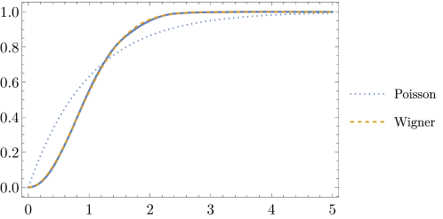
Fig. 7 shows quite clearly that the Hamiltonian of Fig. 3 in the main text is not integrable. Indeed, the cumulative distribution of the energy level spacing is in excellent agreement with the Wigner-Dyson distribution.
Refer to caption
Figure 7: Cumulative distribution of the unfolded energy level spacing in a sector of 𝐇𝐇\boldsymbol{\mathbf{H}} with J=1,γ=0.5,w=0.7,Δ=0,Dz=0.6,hz=0formulae-sequence𝐽1formulae-sequence𝛾0.5formulae-sequence𝑤0.7formulae-sequenceΔ0formulae-sequencesuperscript𝐷𝑧0.6superscript𝑧0J=1,\gamma=0.5,w=0.7,\Delta=0,D^{z}=0.6,h^{z}=0 in a chain with 202020 spins. The data are shown as a solid curve; the dotted and dashed curves are the (normalised) Poisson and Wigner-Dyson predictions expected in integrable and generic models, respectively.

Appendix B Localised excitations

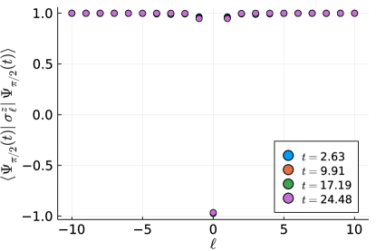
The main exception to the development of macroscopic entanglement after a local projective measurement is when the pre-measurement state is the ground state in a disordered phase. We consider, for example, the dual XXZ Hamiltonian H=𝝈1x1𝝈z8𝝈+1xhz2𝝈z𝐻subscriptsubscriptsuperscript𝝈𝑥11subscriptsuperscript𝝈𝑧8subscriptsuperscript𝝈𝑥1superscript𝑧2subscriptsuperscript𝝈𝑧H=\sum_{\ell}\boldsymbol{\mathbf{\sigma}}^{x}_{\ell-1}\frac{1-\boldsymbol{\mathbf{\sigma}}^{z}_{\ell}}{8}\boldsymbol{\mathbf{\sigma}}^{x}_{\ell+1}-\frac{h^{z}}{2}\boldsymbol{\mathbf{\sigma}}^{z}_{\ell}. If the intensity of the magnetic field |hz|superscript𝑧|h^{z}| is larger than 1212\frac{1}{2}, the pre-measurement state becomes the ground state, and a spin flip excites only local modes that do not spread with time — see Fig. 8.
Refer to caption
Figure 8: The magnetization does not change for any accessible time. The fact that the magnetization is maximal except for a few sites around the origin tells us that most of the system is in the |ket\ket{\Uparrow} state.

Appendix C Absence of macroscopic effects in models with a U(1)𝑈1U(1) symmetry

In this section we prove that a state |ΨketΨ\ket{\Psi} obtained by time evolution under a U(1)𝑈1U(1)-symmetric Hamiltonian after a local perturbation to |ket\ket{\Uparrow} is macroscopically equivalent to |ket\ket{\Uparrow}; that is to say, the quantity Ψ|𝐎|Ψ|𝐎|quantum-operator-productΨ𝐎Ψquantum-operator-product𝐎\braket{\Psi}{\boldsymbol{\mathbf{O}}}{\Psi}-\braket{\Uparrow}{\boldsymbol{\mathbf{O}}}{\Uparrow} is subextensive for any translational-invariant operator 𝐎=𝐎A𝐎subscriptsubscript𝐎subscript𝐴\boldsymbol{\mathbf{O}}=\sum_{\ell}\boldsymbol{\mathbf{O}}_{A_{\ell}}, with 𝐎Asubscript𝐎subscript𝐴\boldsymbol{\mathbf{O}}_{A_{\ell}} local operators. We also prove that the variance of any of such operators 𝐎𝐎\boldsymbol{\mathbf{O}} with respect to the state |ΨketΨ\ket{\Psi} grows at most linearly with system |Ωϵ(t)|subscriptΩitalic-ϵ𝑡|\Omega_{\epsilon}(t)|, ruling out the possibility to obtain a macroscopically entangled state from time-evolution of a locally-perturbed |ket\ket{\Uparrow}.

Let us denote by |ΨsketsubscriptΨ𝑠\ket{\Psi_{s}} a state obtained by flipping s𝑠s spins in |ket\ket{\Uparrow}, or linear combination of them. We start by observing that, if 𝐒zsuperscript𝐒𝑧\boldsymbol{\mathbf{S}}^{z} is conserved, the state time-evolves as

|Ψs(t)=n1<n2<<nsw{n}(t)𝝈n1𝝈n2𝝈ns|,ketsubscriptΨ𝑠𝑡subscriptsubscript𝑛1subscript𝑛2subscript𝑛𝑠subscript𝑤𝑛𝑡superscriptsubscript𝝈subscript𝑛1superscriptsubscript𝝈subscript𝑛2superscriptsubscript𝝈subscript𝑛𝑠ket\ket{\Psi_{s}(t)}=\sum_{n_{1}<n_{2}<...<n_{s}}w_{\{n\}}(t)\boldsymbol{\mathbf{\sigma}}_{n_{1}}^{-}\boldsymbol{\mathbf{\sigma}}_{n_{2}}^{-}...\boldsymbol{\mathbf{\sigma}}_{n_{s}}^{-}\ket{\Uparrow}\,,

for some coefficients such that n1<n2<<ns|w{n}|2=1subscriptsubscript𝑛1subscript𝑛2subscript𝑛𝑠superscriptsubscript𝑤𝑛21\sum_{n_{1}<n_{2}<...<n_{s}}|w_{\{n\}}|^{2}=1. Let 𝐎Asubscript𝐎subscript𝐴\boldsymbol{\mathbf{O}}_{A_{\ell}} be an operator with support in A𝐴A, where Asubscript𝐴A_{\ell} is a set of |A|𝐴|A| adjacent sites starting with the \ell-th spin: A={,,+|A|1}𝐴conditional-setlimit-fromconditional𝐴1A=\{\ell,...,\ell+|A|-1\}. We have

Ψs(t)|𝐎A|Ψs(t)|𝐎A|=i=1sn1<<nsnkAk=i(ninkA,k{i}w{n}(t)w{n},nini(t)|𝝈ni+𝐎A𝝈ni||w{n}(t)|2|𝐎A|)+i=1s1n1<<nsnkAk{i,i+1}(ni<ni+1nkA,k{i,i+1}w{n}(t)w{n},ninini+1ni+1(t)|𝝈ni+𝝈ni+1+𝐎A𝝈ni𝝈ni+1||w{n}(t)|2|𝐎A|)++n1<<nsnkA,k{1,,s}(n1<<nsnkA,k{1,,s}w{n}(t)w{n}(t)|𝝈n1+𝝈ns+𝐎A𝝈n1𝝈ns||w{n}(t)|2|𝐎A|).quantum-operator-productsubscriptΨ𝑠𝑡subscript𝐎subscript𝐴subscriptΨ𝑠𝑡quantum-operator-productsubscript𝐎subscript𝐴superscriptsubscript𝑖1𝑠subscriptsubscript𝑛1subscript𝑛𝑠subscript𝑛𝑘subscript𝐴𝑘𝑖subscriptsuperscriptsubscript𝑛𝑖formulae-sequencesuperscriptsubscript𝑛𝑘subscript𝐴for-all𝑘𝑖superscriptsubscript𝑤𝑛𝑡subscript𝑤𝑛subscript𝑛𝑖subscriptsuperscript𝑛𝑖𝑡quantum-operator-productsubscriptsuperscript𝝈subscriptsuperscript𝑛𝑖subscript𝐎subscript𝐴subscriptsuperscript𝝈subscript𝑛𝑖superscriptsubscript𝑤𝑛𝑡2quantum-operator-productsubscript𝐎subscript𝐴superscriptsubscript𝑖1𝑠1subscriptsubscript𝑛1subscript𝑛𝑠subscript𝑛𝑘subscript𝐴𝑘𝑖𝑖1subscriptsuperscriptsubscript𝑛𝑖subscriptsuperscript𝑛𝑖1formulae-sequencesubscriptsuperscript𝑛𝑘subscript𝐴for-all𝑘𝑖𝑖1superscriptsubscript𝑤𝑛𝑡subscript𝑤𝑛subscript𝑛𝑖subscriptsuperscript𝑛𝑖subscript𝑛𝑖1subscriptsuperscript𝑛𝑖1𝑡quantum-operator-productsubscriptsuperscript𝝈subscriptsuperscript𝑛𝑖subscriptsuperscript𝝈subscriptsuperscript𝑛𝑖1subscript𝐎subscript𝐴subscriptsuperscript𝝈subscript𝑛𝑖subscriptsuperscript𝝈subscript𝑛𝑖1superscriptsubscript𝑤𝑛𝑡2quantum-operator-productsubscript𝐎subscript𝐴subscriptsubscript𝑛1subscript𝑛𝑠formulae-sequencesubscript𝑛𝑘subscript𝐴for-all𝑘1𝑠subscriptsubscriptsuperscript𝑛1subscriptsuperscript𝑛𝑠formulae-sequencesubscriptsuperscript𝑛𝑘subscript𝐴for-all𝑘1𝑠superscriptsubscript𝑤𝑛𝑡subscript𝑤superscript𝑛𝑡quantum-operator-productsubscriptsuperscript𝝈superscriptsubscript𝑛1subscriptsuperscript𝝈superscriptsubscript𝑛𝑠subscript𝐎subscript𝐴subscriptsuperscript𝝈subscript𝑛1subscriptsuperscript𝝈subscript𝑛𝑠superscriptsubscript𝑤𝑛𝑡2quantum-operator-productsubscript𝐎subscript𝐴\braket{\Psi_{s}(t)}{\boldsymbol{\mathbf{O}}_{A_{\ell}}}{\Psi_{s}(t)}-\braket{\Uparrow}{\boldsymbol{\mathbf{O}}_{A_{\ell}}}{\Uparrow}\\ =\sum_{i=1}^{s}\sum_{\begin{subarray}{c}n_{1}<...<n_{s}\\ n_{k}\in A_{\ell}\Leftrightarrow k=i\end{subarray}}\biggl{(}\sum_{\begin{subarray}{c}n_{i}^{\prime}\\ n_{k}^{\prime}\in A_{\ell},\forall k\in\{i\}\end{subarray}}w_{\{n\}}^{*}(t)w_{\{n\},n_{i}\rightarrow n^{\prime}_{i}}(t)\braket{\Uparrow}{\boldsymbol{\mathbf{\sigma}}^{+}_{n^{\prime}_{i}}\boldsymbol{\mathbf{O}}_{A_{\ell}}\boldsymbol{\mathbf{\sigma}}^{-}_{n_{i}}}{\Uparrow}-|w_{\{n\}}(t)|^{2}\braket{\Uparrow}{\boldsymbol{\mathbf{O}}_{A_{\ell}}}{\Uparrow}\biggr{)}\\ +\sum_{i=1}^{s-1}\sum_{\begin{subarray}{c}n_{1}<...<n_{s}\\ n_{k}\in A_{\ell}\Leftrightarrow k\in\{i,i+1\}\end{subarray}}\biggl{(}\sum_{\begin{subarray}{c}n_{i}^{\prime}<n^{\prime}_{i+1}\\ n^{\prime}_{k}\in A_{\ell},\forall k\in\{i,i+1\}\end{subarray}}w_{\{n\}}^{*}(t)w_{\begin{subarray}{c}\{n\},n_{i}\rightarrow n^{\prime}_{i}\\ n_{i+1}\rightarrow n^{\prime}_{i+1}\end{subarray}}(t)\braket{\Uparrow}{\boldsymbol{\mathbf{\sigma}}^{+}_{n^{\prime}_{i}}\boldsymbol{\mathbf{\sigma}}^{+}_{n^{\prime}_{i+1}}\boldsymbol{\mathbf{O}}_{A_{\ell}}\boldsymbol{\mathbf{\sigma}}^{-}_{n_{i}}\boldsymbol{\mathbf{\sigma}}^{-}_{n_{i+1}}}{\Uparrow}-|w_{\{n\}}(t)|^{2}\braket{\Uparrow}{\boldsymbol{\mathbf{O}}_{A_{\ell}}}{\Uparrow}\biggr{)}\\ +...+\sum_{\begin{subarray}{c}n_{1}<...<n_{s}\\ n_{k}\in A_{\ell},\forall k\in\{1,...,s\}\end{subarray}}\biggl{(}\sum_{\begin{subarray}{c}n^{\prime}_{1}<...<n^{\prime}_{s}\\ n^{\prime}_{k}\in A_{\ell},\forall k\in\{1,...,s\}\end{subarray}}w_{\{n\}}^{*}(t)w_{\{n^{\prime}\}}(t)\braket{\Uparrow}{\boldsymbol{\mathbf{\sigma}}^{+}_{n_{1}^{\prime}}...\boldsymbol{\mathbf{\sigma}}^{+}_{n_{s}^{\prime}}\boldsymbol{\mathbf{O}}_{A_{\ell}}\boldsymbol{\mathbf{\sigma}}^{-}_{n_{1}}...\boldsymbol{\mathbf{\sigma}}^{-}_{n_{s}}}{\Uparrow}-|w_{\{n\}}(t)|^{2}\braket{\Uparrow}{\boldsymbol{\mathbf{O}}_{A_{\ell}}}{\Uparrow}\biggr{)}\,. (23)

An upper bound for the absolute value of the left hand side of the equation is obtained using v|𝐎|v𝐎v|vquantum-operator-product𝑣𝐎𝑣norm𝐎inner-product𝑣𝑣\braket{v}{\boldsymbol{\mathbf{O}}}{v}\leq\parallel\boldsymbol{\mathbf{O}}\parallel\braket{v}{v}, where 𝐎norm𝐎\parallel\boldsymbol{\mathbf{O}}\parallel denotes the operator norm, indeed we have

|Ψs(t)|𝐎A|Ψs(t)|𝐎A||2𝐎A(i=1sn1<<nsnkAk=i|w{n}(t)|2+i=1s1n1<<nsnkAk{i,i+1}|w{n}(t)|2++n1<<nsnkA,k{1,,s}|w{n}(t)|2)2𝐎Ai=1sn1<<nsniA|w{n}(t)|2,quantum-operator-productsubscriptΨ𝑠𝑡subscript𝐎subscript𝐴subscriptΨ𝑠𝑡quantum-operator-productsubscript𝐎subscript𝐴2delimited-∥∥subscript𝐎subscript𝐴superscriptsubscript𝑖1𝑠subscriptsubscript𝑛1subscript𝑛𝑠subscript𝑛𝑘subscript𝐴𝑘𝑖superscriptsubscript𝑤𝑛𝑡2superscriptsubscript𝑖1𝑠1subscriptsubscript𝑛1subscript𝑛𝑠subscript𝑛𝑘subscript𝐴𝑘𝑖𝑖1superscriptsubscript𝑤𝑛𝑡2subscriptsubscript𝑛1subscript𝑛𝑠formulae-sequencesubscript𝑛𝑘subscript𝐴for-all𝑘1𝑠superscriptsubscript𝑤𝑛𝑡22delimited-∥∥subscript𝐎subscript𝐴superscriptsubscript𝑖1𝑠subscriptsubscript𝑛1subscript𝑛𝑠subscript𝑛𝑖subscript𝐴superscriptsubscript𝑤𝑛𝑡2|\braket{\Psi_{s}(t)}{\boldsymbol{\mathbf{O}}_{A_{\ell}}}{\Psi_{s}(t)}-\braket{\Uparrow}{\boldsymbol{\mathbf{O}}_{A_{\ell}}}{\Uparrow}|\leq\\ \leq 2\parallel\boldsymbol{\mathbf{O}}_{A_{\ell}}\parallel\left(\sum_{i=1}^{s}\sum_{\begin{subarray}{c}n_{1}<...<n_{s}\\ n_{k}\in A_{\ell}\Leftrightarrow k=i\end{subarray}}|w_{\{n\}}(t)|^{2}+\sum_{i=1}^{s-1}\sum_{\begin{subarray}{c}n_{1}<...<n_{s}\\ n_{k}\in A_{\ell}\Leftrightarrow k\in\{i,i+1\}\end{subarray}}|w_{\{n\}}(t)|^{2}+...+\sum_{\begin{subarray}{c}n_{1}<...<n_{s}\\ n_{k}\in A_{\ell},\forall k\in\{1,...,s\}\end{subarray}}|w_{\{n\}}(t)|^{2}\right)\leq\\ \leq 2\parallel\boldsymbol{\mathbf{O}}_{A_{\ell}}\parallel\sum_{i=1}^{s}\sum_{\begin{subarray}{c}n_{1}<...<n_{s}\\ n_{i}\in A_{\ell}\end{subarray}}|w_{\{n\}}(t)|^{2}\,, (24)

where the last step is not an equality because there are some coefficients w𝑤w that are counted more than once in the last line (e.g., if we take s=2𝑠2s=2 and A={,+1}subscript𝐴1A_{\ell}=\{\ell,\ell+1\}, there is originally just one term |w,+1|2superscriptsubscript𝑤12|w_{\ell,\ell+1}|^{2}, coming from the sum n1<<nsnkA,k{1,,s}subscriptsubscript𝑛1subscript𝑛𝑠formulae-sequencesubscript𝑛𝑘subscript𝐴for-all𝑘1𝑠\sum_{\begin{subarray}{c}n_{1}<...<n_{s}\\ n_{k}\in A_{\ell},\forall k\in\{1,...,s\}\end{subarray}}, but the sum i=1sn1<<nsniAsuperscriptsubscript𝑖1𝑠subscriptsubscript𝑛1subscript𝑛𝑠subscript𝑛𝑖subscript𝐴\sum_{i=1}^{s}\sum_{\begin{subarray}{c}n_{1}<...<n_{s}\\ n_{i}\in A_{\ell}\end{subarray}} has two of such terms, that we get for i=𝑖i=\ell and i=+1𝑖1i=\ell+1). Let us now consider the corresponding translational-invariant extensive operator 𝐎=Ωϵ(t)𝐎A𝐎subscriptsubscriptΩitalic-ϵ𝑡subscript𝐎subscript𝐴\boldsymbol{\mathbf{O}}=\sum_{\ell\in\Omega_{\epsilon}(t)}\boldsymbol{\mathbf{O}}_{A_{\ell}}, where here ΩϵsubscriptΩitalic-ϵ\Omega_{\epsilon} has a generalised definition with respect to the main text, since we want it to include all the light cones steaming from each spin flip. This gives

|Ψs(t)|𝐎|Ψs(t)|𝐎||Ωϵ(t)|Ψs(t)|𝐎A|Ψs(t)|𝐎A||2𝐎A1Ωϵ(t)i=1sn1<<nsniA|w{n}(t)|22𝐎A1|A|i=1sn1<<ns|w{n}(t)|2=2s𝐎A1|A|,quantum-operator-productsubscriptΨ𝑠𝑡𝐎subscriptΨ𝑠𝑡quantum-operator-product𝐎subscriptsubscriptΩitalic-ϵ𝑡quantum-operator-productsubscriptΨ𝑠𝑡subscript𝐎subscript𝐴subscriptΨ𝑠𝑡quantum-operator-productsubscript𝐎subscript𝐴2delimited-∥∥subscript𝐎subscript𝐴1subscriptsubscriptΩitalic-ϵ𝑡superscriptsubscript𝑖1𝑠subscriptsubscript𝑛1subscript𝑛𝑠subscript𝑛𝑖subscript𝐴superscriptsubscript𝑤𝑛𝑡2less-than-or-similar-to2delimited-∥∥subscript𝐎subscript𝐴1𝐴superscriptsubscript𝑖1𝑠subscriptsubscript𝑛1subscript𝑛𝑠superscriptsubscript𝑤𝑛𝑡22𝑠delimited-∥∥subscript𝐎subscript𝐴1𝐴|\braket{\Psi_{s}(t)}{\boldsymbol{\mathbf{O}}}{\Psi_{s}(t)}-\braket{\Uparrow}{\boldsymbol{\mathbf{O}}}{\Uparrow}|\leq\sum_{\ell\in\Omega_{\epsilon}(t)}|\braket{\Psi_{s}(t)}{\boldsymbol{\mathbf{O}}_{A_{\ell}}}{\Psi_{s}(t)}-\braket{\Uparrow}{\boldsymbol{\mathbf{O}}_{A_{\ell}}}{\Uparrow}|\leq\\ \leq 2\parallel\boldsymbol{\mathbf{O}}_{A_{1}}\parallel\sum_{\ell\in\Omega_{\epsilon}(t)}\sum_{i=1}^{s}\sum_{\begin{subarray}{c}n_{1}<...<n_{s}\\ n_{i}\in A_{\ell}\end{subarray}}|w_{\{n\}}(t)|^{2}\lesssim 2\parallel\boldsymbol{\mathbf{O}}_{A_{1}}\parallel|A|\sum_{i=1}^{s}\sum_{n_{1}<...<n_{s}}|w_{\{n\}}(t)|^{2}=2s\parallel\boldsymbol{\mathbf{O}}_{A_{1}}\parallel|A|\,, (25)

where we used translational invariance and less-than-or-similar-to\lesssim rather than \leq because Ωϵ(t)subscriptΩitalic-ϵ𝑡\Omega_{\epsilon}(t) is only approximately pure. This shows that |Ψs(t)ketsubscriptΨ𝑠𝑡\ket{\Psi_{s}(t)} and |ket\ket{\Uparrow} are macroscopically indistinguishable for any time t𝑡t.

We want now to extend the result to the square of the operator. We follow the same steps:

Ψs(t)|𝐎A𝐎A|Ψs(t)|𝐎A𝐎A|=i=1sn1<<nsnkAAk=i(ninkAA,k{i}w{n}(t)w{n},nini(t)|𝝈ni+𝐎A𝐎A𝝈ni||w{n}(t)|2|𝐎A𝐎A|)+i<j=1sn1<<nsnkAAk{i,j}(ni<njnkAA,k{i,j}w{n}(t)w{n},nininjnj(t)|𝝈ni+𝝈nj+𝐎A𝐎A𝝈ni𝝈nj|+|w{n}(t)|2|𝐎A𝐎A|)++n1<<nsnkAA,k{1,,s}(n1<<nsnkAA,k{1,,s}w{n}(t)w{n}(t)××|𝝈n1+𝝈ns+𝐎A𝐎A𝝈n1𝝈ns||w{n}(t)|2|𝐎A𝐎A|),\braket{\Psi_{s}(t)}{\boldsymbol{\mathbf{O}}_{A_{\ell}}\boldsymbol{\mathbf{O}}_{A_{\ell^{\prime}}}}{\Psi_{s}(t)}-\braket{\Uparrow}{\boldsymbol{\mathbf{O}}_{A_{\ell}}\boldsymbol{\mathbf{O}}_{A_{\ell^{\prime}}}}{\Uparrow}\\ =\sum_{i=1}^{s}\sum_{\begin{subarray}{c}n_{1}<...<n_{s}\\ n_{k}\in A_{\ell}\cup A_{\ell^{\prime}}\Leftrightarrow k=i\end{subarray}}\biggl{(}\sum_{\begin{subarray}{c}n_{i}^{\prime}\\ n_{k}^{\prime}\in A_{\ell}\cup A_{\ell^{\prime}},\forall k\in\{i\}\end{subarray}}w_{\{n\}}^{*}(t)w_{\{n\},n_{i}\rightarrow n^{\prime}_{i}}(t)\braket{\Uparrow}{\boldsymbol{\mathbf{\sigma}}^{+}_{n^{\prime}_{i}}\boldsymbol{\mathbf{O}}_{A_{\ell}}\boldsymbol{\mathbf{O}}_{A_{\ell^{\prime}}}\boldsymbol{\mathbf{\sigma}}^{-}_{n_{i}}}{\Uparrow}-|w_{\{n\}}(t)|^{2}\braket{\Uparrow}{\boldsymbol{\mathbf{O}}_{A_{\ell}}\boldsymbol{\mathbf{O}}_{A_{\ell^{\prime}}}}{\Uparrow}\biggr{)}\\ +\sum_{i<j=1}^{s}\sum_{\begin{subarray}{c}n_{1}<...<n_{s}\\ n_{k}\in A_{\ell}\cup A_{\ell^{\prime}}\Leftrightarrow k\in\{i,j\}\end{subarray}}\biggl{(}\sum_{\begin{subarray}{c}n_{i}^{\prime}<n^{\prime}_{j}\\ n^{\prime}_{k}\in A_{\ell}\cup A_{\ell^{\prime}},\forall k\in\{i,j\}\end{subarray}}w_{\{n\}}^{*}(t)w_{\begin{subarray}{c}\{n\},n_{i}\rightarrow n^{\prime}_{i}\\ n_{j}\rightarrow n^{\prime}_{j}\end{subarray}}(t)\braket{\Uparrow}{\boldsymbol{\mathbf{\sigma}}^{+}_{n^{\prime}_{i}}\boldsymbol{\mathbf{\sigma}}^{+}_{n^{\prime}_{j}}\boldsymbol{\mathbf{O}}_{A_{\ell}}\boldsymbol{\mathbf{O}}_{A_{\ell^{\prime}}}\boldsymbol{\mathbf{\sigma}}^{-}_{n_{i}}\boldsymbol{\mathbf{\sigma}}^{-}_{n_{j}}}{\Uparrow}+\\ -|w_{\{n\}}(t)|^{2}\braket{\Uparrow}{\boldsymbol{\mathbf{O}}_{A_{\ell}}\boldsymbol{\mathbf{O}}_{A_{\ell^{\prime}}}}{\Uparrow}\biggr{)}+\dots+\sum_{\begin{subarray}{c}n_{1}<...<n_{s}\\ n_{k}\in A_{\ell}\cup A_{\ell^{\prime}},\forall k\in\{1,...,s\}\end{subarray}}\biggl{(}\sum_{\begin{subarray}{c}n^{\prime}_{1}<...<n^{\prime}_{s}\\ n^{\prime}_{k}\in A_{\ell}\cup A_{\ell^{\prime}},\forall k\in\{1,...,s\}\end{subarray}}w_{\{n\}}^{*}(t)w_{\{n^{\prime}\}}(t)\times\\ \times\braket{\Uparrow}{\boldsymbol{\mathbf{\sigma}}^{+}_{n_{1}^{\prime}}...\boldsymbol{\mathbf{\sigma}}^{+}_{n_{s}^{\prime}}\boldsymbol{\mathbf{O}}_{A_{\ell}}\boldsymbol{\mathbf{O}}_{A_{\ell^{\prime}}}\boldsymbol{\mathbf{\sigma}}^{-}_{n_{1}}...\boldsymbol{\mathbf{\sigma}}^{-}_{n_{s}}}{\Uparrow}-|w_{\{n\}}(t)|^{2}\braket{\Uparrow}{\boldsymbol{\mathbf{O}}_{A_{\ell}}\boldsymbol{\mathbf{O}}_{A_{\ell^{\prime}}}}{\Uparrow}\biggr{)}\,, (26)

from which

|Ψs(t)|𝐎A𝐎A|Ψs(t)|𝐎A𝐎A||2𝐎A2i=1sn1<<nsnkAAk=i|w{n}(t)|2++2𝐎A2i<j=1sn1<<nsnkAAk{i,j}|w{n}(t)|2++2𝐎A2n1<<nsnkAA,k{1,,s}|w{n}(t)|22𝐎A2i=1sn1<<nsniAA|w{n}(t)|2,quantum-operator-productsubscriptΨ𝑠𝑡subscript𝐎subscript𝐴subscript𝐎subscript𝐴superscriptsubscriptΨ𝑠𝑡quantum-operator-productsubscript𝐎subscript𝐴subscript𝐎subscript𝐴superscript2superscriptdelimited-∥∥subscript𝐎subscript𝐴2superscriptsubscript𝑖1𝑠subscriptsubscript𝑛1subscript𝑛𝑠subscript𝑛𝑘subscript𝐴subscript𝐴superscript𝑘𝑖superscriptsubscript𝑤𝑛𝑡22superscriptdelimited-∥∥subscript𝐎subscript𝐴2superscriptsubscript𝑖𝑗1𝑠subscriptsubscript𝑛1subscript𝑛𝑠subscript𝑛𝑘subscript𝐴subscript𝐴superscript𝑘𝑖𝑗superscriptsubscript𝑤𝑛𝑡22superscriptdelimited-∥∥subscript𝐎subscript𝐴2subscriptsubscript𝑛1subscript𝑛𝑠formulae-sequencesubscript𝑛𝑘subscript𝐴subscript𝐴superscriptfor-all𝑘1𝑠superscriptsubscript𝑤𝑛𝑡22superscriptdelimited-∥∥subscript𝐎subscript𝐴2superscriptsubscript𝑖1𝑠subscriptsubscript𝑛1subscript𝑛𝑠subscript𝑛𝑖subscript𝐴subscript𝐴superscriptsuperscriptsubscript𝑤𝑛𝑡2|\braket{\Psi_{s}(t)}{\boldsymbol{\mathbf{O}}_{A_{\ell}}\boldsymbol{\mathbf{O}}_{A_{\ell^{\prime}}}}{\Psi_{s}(t)}-\braket{\Uparrow}{\boldsymbol{\mathbf{O}}_{A_{\ell}}\boldsymbol{\mathbf{O}}_{A_{\ell^{\prime}}}}{\Uparrow}|\leq 2\parallel\boldsymbol{\mathbf{O}}_{A_{\ell}}\parallel^{2}\sum_{i=1}^{s}\sum_{\begin{subarray}{c}n_{1}<...<n_{s}\\ n_{k}\in A_{\ell}\cup A_{\ell^{\prime}}\Leftrightarrow k=i\end{subarray}}|w_{\{n\}}(t)|^{2}+\\ +2\parallel\boldsymbol{\mathbf{O}}_{A_{\ell}}\parallel^{2}\sum_{i<j=1}^{s}\sum_{\begin{subarray}{c}n_{1}<...<n_{s}\\ n_{k}\in A_{\ell}\cup A_{\ell^{\prime}}\Leftrightarrow k\in\{i,j\}\end{subarray}}|w_{\{n\}}(t)|^{2}+\dots+2\parallel\boldsymbol{\mathbf{O}}_{A_{\ell}}\parallel^{2}\sum_{\begin{subarray}{c}n_{1}<...<n_{s}\\ n_{k}\in A_{\ell}\cup A_{\ell^{\prime}},\forall k\in\{1,...,s\}\end{subarray}}|w_{\{n\}}(t)|^{2}\\ \leq 2\parallel\boldsymbol{\mathbf{O}}_{A_{\ell}}\parallel^{2}\sum_{i=1}^{s}\sum_{\begin{subarray}{c}n_{1}<...<n_{s}\\ n_{i}\in A_{\ell}\cup A_{\ell^{\prime}}\end{subarray}}|w_{\{n\}}(t)|^{2}\,, (27)

and finally

|Ψs(t)|𝐎2|Ψs(t)|𝐎2||,Ωϵ(t)|Ψs(t)|𝐎A𝐎A|Ψs(t)|𝐎A𝐎A||2𝐎A12,Ωϵ(t)i=1sn1<<nsniAA|w{n}(t)|24𝐎A12,Ωϵ(t)i=1sn1<<nsniA|w{n}(t)|24𝐎A12|A||Ωϵ(t)|i=1sn1<<ns|w{n}(t)|2=4s𝐎A12|A||Ωϵ(t)|.quantum-operator-productsubscriptΨ𝑠𝑡superscript𝐎2subscriptΨ𝑠𝑡quantum-operator-productsuperscript𝐎2subscriptsuperscriptsubscriptΩitalic-ϵ𝑡quantum-operator-productsubscriptΨ𝑠𝑡subscript𝐎subscript𝐴subscript𝐎subscript𝐴superscriptsubscriptΨ𝑠𝑡quantum-operator-productsubscript𝐎subscript𝐴subscript𝐎subscript𝐴superscript2superscriptdelimited-∥∥subscript𝐎subscript𝐴12subscriptsuperscriptsubscriptΩitalic-ϵ𝑡superscriptsubscript𝑖1𝑠subscriptsubscript𝑛1subscript𝑛𝑠subscript𝑛𝑖subscript𝐴subscript𝐴superscriptsuperscriptsubscript𝑤𝑛𝑡24superscriptdelimited-∥∥subscript𝐎subscript𝐴12subscriptsuperscriptsubscriptΩitalic-ϵ𝑡superscriptsubscript𝑖1𝑠subscriptsubscript𝑛1subscript𝑛𝑠subscript𝑛𝑖subscript𝐴superscriptsubscript𝑤𝑛𝑡2less-than-or-similar-to4superscriptdelimited-∥∥subscript𝐎subscript𝐴12𝐴subscriptΩitalic-ϵ𝑡superscriptsubscript𝑖1𝑠subscriptsubscript𝑛1subscript𝑛𝑠superscriptsubscript𝑤𝑛𝑡24𝑠superscriptdelimited-∥∥subscript𝐎subscript𝐴12𝐴subscriptΩitalic-ϵ𝑡|\braket{\Psi_{s}(t)}{\boldsymbol{\mathbf{O}}^{2}}{\Psi_{s}(t)}-\braket{\Uparrow}{\boldsymbol{\mathbf{O}}^{2}}{\Uparrow}|\leq\sum_{\ell,\ell^{\prime}\in\Omega_{\epsilon}(t)}|\braket{\Psi_{s}(t)}{\boldsymbol{\mathbf{O}}_{A_{\ell}}\boldsymbol{\mathbf{O}}_{A_{\ell^{\prime}}}}{\Psi_{s}(t)}-\braket{\Uparrow}{\boldsymbol{\mathbf{O}}_{A_{\ell}}\boldsymbol{\mathbf{O}}_{A_{\ell^{\prime}}}}{\Uparrow}|\\ \leq 2\parallel\boldsymbol{\mathbf{O}}_{A_{1}}\parallel^{2}\sum_{\ell,\ell^{\prime}\in\Omega_{\epsilon}(t)}\sum_{i=1}^{s}\sum_{\begin{subarray}{c}n_{1}<...<n_{s}\\ n_{i}\in A_{\ell}\cup A_{\ell^{\prime}}\end{subarray}}|w_{\{n\}}(t)|^{2}\leq 4\parallel\boldsymbol{\mathbf{O}}_{A_{1}}\parallel^{2}\sum_{\ell,\ell^{\prime}\in\Omega_{\epsilon}(t)}\sum_{i=1}^{s}\sum_{\begin{subarray}{c}n_{1}<...<n_{s}\\ n_{i}\in A_{\ell}\end{subarray}}|w_{\{n\}}(t)|^{2}\\ \lesssim 4\parallel\boldsymbol{\mathbf{O}}_{A_{1}}\parallel^{2}|A||\Omega_{\epsilon}(t)|\sum_{i=1}^{s}\sum_{n_{1}<...<n_{s}}|w_{\{n\}}(t)|^{2}=4s\parallel\boldsymbol{\mathbf{O}}_{A_{1}}\parallel^{2}|A||\Omega_{\epsilon}(t)|\,. (28)

This shows that the variance of the any operator 𝐎𝐎\boldsymbol{\mathbf{O}} on the state |Ψs(t)ketsubscriptΨ𝑠𝑡\ket{\Psi_{s}(t)} coincides with the one on the state |ket\ket{\Uparrow} modulo corrections of order 𝒪(|Ωϵ(t)|)𝒪subscriptΩitalic-ϵ𝑡\mathcal{O}(|\Omega_{\epsilon}(t)|). Since |ket\ket{\Uparrow} is a state for which clustering of correlations holds and his variance cannot be larger than system’s size, we obtain that the state |Ψs(t)ketsubscriptΨ𝑠𝑡\ket{\Psi_{s}(t)} has the same properties, implying that it is not macroscopically entangled. Our proof can be easily generalised to any power of the operator, but higher powers are not needed to our purposes.

We now extend the results above to more general states. We consider, first, the quantity Ψs|𝐎|Ψsquantum-operator-productsubscriptΨsuperscript𝑠𝐎subscriptΨ𝑠\braket{\Psi_{s^{\prime}}}{\boldsymbol{\mathbf{O}}}{\Psi_{s}}, ss𝑠superscript𝑠s\neq s^{\prime}, for two different states |ΨsketsubscriptΨ𝑠\ket{\Psi_{s}} and |ΨsketsubscriptΨsuperscript𝑠\ket{\Psi_{s^{\prime}}}. Without loss of generality, we can assume s>s𝑠superscript𝑠s>s^{\prime}. We start from

|Ψs|𝐎|Ψs|Ωϵ(t)n1<<nsn1<<ns||𝝈n1+𝝈ns+𝐎A𝝈n1𝝈ns|||w{n}(t)||w{n}(t)|,quantum-operator-productsubscriptΨsuperscript𝑠𝐎subscriptΨ𝑠subscriptsubscriptΩitalic-ϵ𝑡subscriptsubscriptsuperscript𝑛1subscriptsuperscript𝑛superscript𝑠subscriptsubscript𝑛1subscript𝑛𝑠quantum-operator-productsubscriptsuperscript𝝈subscriptsuperscript𝑛1subscriptsuperscript𝝈subscriptsuperscript𝑛superscript𝑠subscript𝐎subscript𝐴subscriptsuperscript𝝈subscript𝑛1subscriptsuperscript𝝈subscript𝑛𝑠subscriptsuperscript𝑤superscript𝑛𝑡subscript𝑤𝑛𝑡|\braket{\Psi_{s^{\prime}}}{\boldsymbol{\mathbf{O}}}{\Psi_{s}}|\leq\sum_{\ell\in\Omega_{\epsilon}(t)}\sum_{n^{\prime}_{1}<...<n^{\prime}_{s^{\prime}}}\sum_{n_{1}<...<n_{s}}|\braket{\Uparrow}{\boldsymbol{\mathbf{\sigma}}^{+}_{n^{\prime}_{1}}...\boldsymbol{\mathbf{\sigma}}^{+}_{n^{\prime}_{s^{\prime}}}\boldsymbol{\mathbf{O}}_{A_{\ell}}\boldsymbol{\mathbf{\sigma}}^{-}_{n_{1}}...\boldsymbol{\mathbf{\sigma}}^{-}_{n_{s}}}{\Uparrow}||w^{\prime}_{\{n^{\prime}\}}(t)||w_{\{n\}}(t)|, (29)

and rewrite the sums regrouping them, for fixed \ell, according to how many of the primed indices {n}superscript𝑛\{n^{\prime}\} are outside the set Asubscript𝐴A_{\ell}. This is a number p𝑝p that goes from 0 to ssuperscript𝑠s^{\prime}. In order to get a non-zero contribution, the number of indices {n}𝑛\{n\} outside Asubscript𝐴A_{\ell} should also be p𝑝p. The number of indices {n}Asuperscript𝑛subscript𝐴\{n^{\prime}\}\in A_{\ell} is then sp{0,,s}superscript𝑠𝑝0superscript𝑠s^{\prime}-p\in\{0,...,s^{\prime}\}, while the number of indices {n}A𝑛subscript𝐴\{n\}\in A_{\ell} is sp{ss,,s}𝑠𝑝𝑠superscript𝑠𝑠s-p\in\{s-s^{\prime},...,s\}; note that there is no contribution from |A|<spsubscript𝐴𝑠𝑝|A_{\ell}|<s-p. For given p𝑝p, there are p+1𝑝1p+1 distinct subsets of consecutive n𝑛n that can be in Asubscript𝐴A_{\ell} (they are characterised by the position of the first element of the subset); to keep track of this fact, we introduce a sum over an index j𝑗j, such that the index njsubscript𝑛𝑗n_{j} is the smallest of the indices {n}A𝑛subscript𝐴\{n\}\in A_{\ell}. Such a decomposition leads to

|Ψs|𝐎|Ψs|Ωϵ(t)p=0sj=1p+1n1<<nsnkAjk<j+spn1<<nspnkA,k{1,,sp}||𝝈n1+𝝈nsp+𝐎A𝝈nj𝝈nj+sp1|||w{n}{nj,,nj+sp1}{n1,,nsp}(t)||w{n}(t)|𝐎Ap=0sj=1p+1Ωϵ(t)n1<<nsnkAjk<j+spn1<<nspnkA,k{1,,sp}|w{n}{nj,,nj+sp1}{n1,,nsp}(t)||w{n}(t)|.quantum-operator-productsubscriptΨsuperscript𝑠𝐎subscriptΨ𝑠subscriptsubscriptΩitalic-ϵ𝑡superscriptsubscript𝑝0superscript𝑠superscriptsubscript𝑗1𝑝1subscriptsubscript𝑛1subscript𝑛𝑠subscript𝑛𝑘subscript𝐴𝑗𝑘𝑗𝑠𝑝subscriptsubscriptsuperscript𝑛1subscriptsuperscript𝑛superscript𝑠𝑝formulae-sequencesubscriptsuperscript𝑛𝑘subscript𝐴for-all𝑘1superscript𝑠𝑝quantum-operator-productsubscriptsuperscript𝝈subscriptsuperscript𝑛1subscriptsuperscript𝝈subscriptsuperscript𝑛superscript𝑠𝑝subscript𝐎subscript𝐴subscriptsuperscript𝝈subscript𝑛𝑗subscriptsuperscript𝝈subscript𝑛𝑗𝑠𝑝1subscriptsuperscript𝑤𝑛subscript𝑛𝑗subscript𝑛𝑗𝑠𝑝1subscriptsuperscript𝑛1subscriptsuperscript𝑛superscript𝑠𝑝𝑡subscript𝑤𝑛𝑡delimited-∥∥subscript𝐎subscript𝐴superscriptsubscript𝑝0superscript𝑠superscriptsubscript𝑗1𝑝1subscriptsubscriptΩitalic-ϵ𝑡subscriptsubscript𝑛1subscript𝑛𝑠subscript𝑛𝑘subscript𝐴𝑗𝑘𝑗𝑠𝑝subscriptsubscriptsuperscript𝑛1subscriptsuperscript𝑛superscript𝑠𝑝formulae-sequencesubscriptsuperscript𝑛𝑘subscript𝐴for-all𝑘1superscript𝑠𝑝subscriptsuperscript𝑤𝑛subscript𝑛𝑗subscript𝑛𝑗𝑠𝑝1subscriptsuperscript𝑛1subscriptsuperscript𝑛superscript𝑠𝑝𝑡subscript𝑤𝑛𝑡|\braket{\Psi_{s^{\prime}}}{\boldsymbol{\mathbf{O}}}{\Psi_{s}}|\leq\sum_{\ell\in\Omega_{\epsilon}(t)}\sum_{p=0}^{s^{\prime}}\sum_{j=1}^{p+1}\sum_{\begin{subarray}{c}n_{1}<...<n_{s}\\ n_{k}\in A_{\ell}\Leftrightarrow j\leq k<j+s-p\end{subarray}}\sum_{\begin{subarray}{c}n^{\prime}_{1}<...<n^{\prime}_{s^{\prime}-p}\\ n^{\prime}_{k}\in A_{\ell},\forall k\in\{1,...,s^{\prime}-p\}\end{subarray}}\\ |\braket{\Uparrow}{\boldsymbol{\mathbf{\sigma}}^{+}_{n^{\prime}_{1}}...\boldsymbol{\mathbf{\sigma}}^{+}_{n^{\prime}_{s^{\prime}-p}}\boldsymbol{\mathbf{O}}_{A_{\ell}}\boldsymbol{\mathbf{\sigma}}^{-}_{n_{j}}...\boldsymbol{\mathbf{\sigma}}^{-}_{n_{j+s-p-1}}}{\Uparrow}||w^{\prime}_{\{n\}\setminus\{n_{j},...,n_{j+s-p-1}\}\cup\{n^{\prime}_{1},...,n^{\prime}_{s^{\prime}-p}\}}(t)||w_{\{n\}}(t)|\leq\\ \leq\parallel\boldsymbol{\mathbf{O}}_{A_{\ell}}\parallel\sum_{p=0}^{s^{\prime}}\sum_{j=1}^{p+1}\sum_{\ell\in\Omega_{\epsilon}(t)}\sum_{\begin{subarray}{c}n_{1}<...<n_{s}\\ n_{k}\in A_{\ell}\Leftrightarrow j\leq k<j+s-p\end{subarray}}\sum_{\begin{subarray}{c}n^{\prime}_{1}<...<n^{\prime}_{s^{\prime}-p}\\ n^{\prime}_{k}\in A_{\ell},\forall k\in\{1,...,s^{\prime}-p\}\end{subarray}}|w^{\prime}_{\{n\}\setminus\{n_{j},...,n_{j+s-p-1}\}\cup\{n^{\prime}_{1},...,n^{\prime}_{s^{\prime}-p}\}}(t)||w_{\{n\}}(t)|. (30)

It is now convenient to write the sum over the indices n,n𝑛superscript𝑛n,n^{\prime} in Asubscript𝐴A_{\ell} in another way. We introduce PkKsuperscriptsubscript𝑃𝑘𝐾P_{k}^{K} as the set of all the k𝑘k-tuples of increasing numbers in {0,,K1}0𝐾1\{0,...,K-1\}. Note that PkKsuperscriptsubscript𝑃𝑘𝐾P_{k}^{K} has (Kk)binomial𝐾𝑘\binom{K}{k} elements. We then have

|Ψs|𝐎|Ψs|𝐎Ap=0sj=1p+1Ωϵ(t)(k1,,ksp)Psp|A|(k1,,ksp)Psp|A|n1<<nj1<A<nj+sp<<ns|w{n1,,nj1,+k1,,+ksp,nj+sp,,ns}(t)||w{n1,,nj1,+k1,,+ksp,nj+sp,,ns(t)|,|\braket{\Psi_{s^{\prime}}}{\boldsymbol{\mathbf{O}}}{\Psi_{s}}|\leq\parallel\boldsymbol{\mathbf{O}}_{A_{\ell}}\parallel\sum_{p=0}^{s^{\prime}}\sum_{j=1}^{p+1}\sum_{\ell\in\Omega_{\epsilon}(t)}\sum_{(k_{1},...,k_{s-p})\in P_{s-p}^{|A|}}\sum_{(k^{\prime}_{1},...,k^{\prime}_{s^{\prime}-p})\in P_{s^{\prime}-p}^{|A|}}\sum_{n_{1}<...<n_{j-1}<A_{\ell}<n_{j+s-p}<...<n_{s}}\\ |w^{\prime}_{\{n_{1},...,n_{j-1},\ell+k^{\prime}_{1},...,\ell+k^{\prime}_{s^{\prime}-p},n_{j+s-p},...,n_{s}\}}(t)||w_{\{n_{1},...,n_{j-1},\ell+k_{1},...,\ell+k_{s-p},n_{j+s-p},...,n_{s}}(t)|, (31)

which we rewrite isolating the term with p=s𝑝superscript𝑠p=s^{\prime} (the case in which all the indices {n}superscript𝑛\{n^{\prime}\} are outside Asubscript𝐴A_{\ell}), which is special:

|Ψs|𝐎|Ψs|𝐎Ap=0s1j=1p+1(k1,,ksp)Psp|A|(k1,,ksp)Psp|A|Ωϵ(t)n1<<nj1<A<nj+sp<<ns|w{n1,,nj1,+k1,,+ksp,nj+sp,,ns}(t)||w{n1,,nj1,+k1,,+ksp,nj+sp,,ns(t)|+𝐎Aj=1s+1(k1,,kss)Pss|A|Ωϵ(t)n1<<nj1<A<nj+ss<<ns|w{n1,,nj1,nj+ss,,ns}(t)||w{n1,,nj1,+k1,,+kss,nj+ss,,ns(t)|.|\braket{\Psi_{s^{\prime}}}{\boldsymbol{\mathbf{O}}}{\Psi_{s}}|\leq\parallel\boldsymbol{\mathbf{O}}_{A_{\ell}}\parallel\sum_{p=0}^{s^{\prime}-1}\sum_{j=1}^{p+1}\sum_{(k_{1},...,k_{s-p})\in P_{s-p}^{|A|}}\sum_{(k^{\prime}_{1},...,k^{\prime}_{s^{\prime}-p})\in P_{s^{\prime}-p}^{|A|}}\sum_{\ell\in\Omega_{\epsilon}(t)}\sum_{n_{1}<...<n_{j-1}<A_{\ell}<n_{j+s-p}<...<n_{s}}\\ |w^{\prime}_{\{n_{1},...,n_{j-1},\ell+k^{\prime}_{1},...,\ell+k^{\prime}_{s^{\prime}-p},n_{j+s-p},...,n_{s}\}}(t)||w_{\{n_{1},...,n_{j-1},\ell+k_{1},...,\ell+k_{s-p},n_{j+s-p},...,n_{s}}(t)|\\ +\parallel\boldsymbol{\mathbf{O}}_{A_{\ell}}\parallel\sum_{j=1}^{s^{\prime}+1}\sum_{(k_{1},...,k_{s-s^{\prime}})\in P_{s-s^{\prime}}^{|A|}}\sum_{\ell\in\Omega_{\epsilon}(t)}\sum_{n_{1}<...<n_{j-1}<A_{\ell}<n_{j+s-s^{\prime}}<...<n_{s}}\\ |w^{\prime}_{\{n_{1},...,n_{j-1},n_{j+s-s^{\prime}},...,n_{s}\}}(t)||w_{\{n_{1},...,n_{j-1},\ell+k_{1},...,\ell+k_{s-s^{\prime}},n_{j+s-s^{\prime}},...,n_{s}}(t)|. (32)

Now, for fixed p,j,{k},{k}𝑝𝑗𝑘superscript𝑘p,j,\{k\},\{k^{\prime}\}, we want to maximize the sums over ,{n}𝑛\ell,\{n\} independently, which gives an upper bound to the full quantity. To that aim, we introduce the following compact notation: for the terms with p<s𝑝superscript𝑠p<s^{\prime}

Ωϵ(t)n1<<nj1<A<nj+sp<<ns|w{n1,,nj1,+k1,,+ksp,nj+sp,,ns}(t)|××|w{n1,,nj1,+k1,,+ksp,nj+sp,,ns(t)|bBWbWb,\sum_{\ell\in\Omega_{\epsilon}(t)}\sum_{n_{1}<...<n_{j-1}<A_{\ell}<n_{j+s-p}<...<n_{s}}|w^{\prime}_{\{n_{1},...,n_{j-1},\ell+k^{\prime}_{1},...,\ell+k^{\prime}_{s^{\prime}-p},n_{j+s-p},...,n_{s}\}}(t)|\times\\ \times|w_{\{n_{1},...,n_{j-1},\ell+k_{1},...,\ell+k_{s-p},n_{j+s-p},...,n_{s}}(t)|\quad\equiv\sum_{b\in B}W^{\prime}_{b}W_{b}\,, (33)

and for the term p=s𝑝superscript𝑠p=s^{\prime}

Ωϵ(t)n1<<nj1<A<nj+ss<<ns|w{n1,,nj1,nj+ss,,ns}(t)||w{n1,,nj1,+k1,,+kss,nj+ss,,ns(t)|Ωϵ(t)cCWcWc,,\sum_{\ell\in\Omega_{\epsilon}(t)}\sum_{n_{1}<...<n_{j-1}<A_{\ell}<n_{j+s-s^{\prime}}<...<n_{s}}|w^{\prime}_{\{n_{1},...,n_{j-1},n_{j+s-s^{\prime}},...,n_{s}\}}(t)||w_{\{n_{1},...,n_{j-1},\ell+k_{1},...,\ell+k_{s-s^{\prime}},n_{j+s-s^{\prime}},...,n_{s}}(t)|\\ \equiv\sum_{\ell\in\Omega_{\epsilon}(t)}\sum_{c\in C}W^{\prime}_{c}W_{c,\ell}\,, (34)

where b𝑏b and c𝑐c regroup all the indices that w𝑤w and wsuperscript𝑤w^{\prime} have in common and W,W𝑊superscript𝑊W,W^{\prime} are a synthetic expression for the coefficients that report only the indices we are interested in; note that in the first case there are as many independent w𝑤w as wsuperscript𝑤w^{\prime}, while, for p=s𝑝superscript𝑠p=s^{\prime}, wsuperscript𝑤w^{\prime} does not depend on \ell anymore. In order to maximize the expressions above, we should take into accounts the constraints n1<<ns|w{n}|2=1subscriptsubscriptsuperscript𝑛1subscriptsuperscript𝑛superscript𝑠superscriptsubscriptsuperscript𝑤superscript𝑛21\sum_{n^{\prime}_{1}<...<n^{\prime}_{s^{\prime}}}|w^{\prime}_{\{n^{\prime}\}}|^{2}=1 and n1<<ns|w{n}|2=1subscriptsubscript𝑛1subscript𝑛𝑠superscriptsubscript𝑤𝑛21\sum_{n_{1}<...<n_{s}}|w_{\{n\}}|^{2}=1. In our search for the maximum, we can use the stronger conditions bBWb2=1subscript𝑏𝐵superscriptsubscript𝑊𝑏21\sum_{b\in B}W_{b}^{2}=1 and bB(Wb)2=1subscript𝑏𝐵superscriptsubscriptsuperscript𝑊𝑏21\sum_{b\in B}(W^{\prime}_{b})^{2}=1 in the first case and cC(Wc)2=1subscript𝑐𝐶superscriptsuperscriptsubscript𝑊𝑐21\sum_{c\in C}(W_{c}^{\prime})^{2}=1 and cC,Ωϵ(t)Wc,2=1subscriptformulae-sequence𝑐𝐶subscriptΩitalic-ϵ𝑡superscriptsubscript𝑊𝑐21\sum_{c\in C,\ell\in\Omega_{\epsilon}(t)}W_{c,\ell}^{2}=1 in the second case, which amount to require that the coefficients that are not involved in the sum are zero (given the original constraint, this maximises the sum because all the terms are positive). Using the method of Lagrange multipliers, one can show that, under these constraints, bBWbWbsubscript𝑏𝐵subscriptsuperscript𝑊𝑏subscript𝑊𝑏\sum_{b\in B}W^{\prime}_{b}W_{b} is maximised by Wb=Wbsubscript𝑊𝑏subscriptsuperscript𝑊𝑏W_{b}=W^{\prime}_{b} and equals 1, while Ωϵ(t)cCWcWc,subscriptsubscriptΩitalic-ϵ𝑡subscript𝑐𝐶subscriptsuperscript𝑊𝑐subscript𝑊𝑐\sum_{\ell\in\Omega_{\epsilon}(t)}\sum_{c\in C}W^{\prime}_{c}W_{c,\ell} has degenerate points of maximum in Wc,=|Ωϵ(t)|1/2Wcsubscript𝑊𝑐superscriptsubscriptΩitalic-ϵ𝑡12subscriptsuperscript𝑊𝑐W_{c,\ell}=|\Omega_{\epsilon}(t)|^{-1/2}W^{\prime}_{c} and gives |Ωϵ(t)|1/2superscriptsubscriptΩitalic-ϵ𝑡12|\Omega_{\epsilon}(t)|^{1/2}. In the end

|Ψs|𝐎|Ψs|𝐎Aj=1s+1(k1,,kss)Pss|A||Ωϵ(t)|1/2+𝒪(|Ωϵ(t)|0)==𝐎A(s+1)(|A|ss)|Ωϵ(t)|1/2+𝒪(|Ωϵ(t)|0).quantum-operator-productsubscriptΨsuperscript𝑠𝐎subscriptΨ𝑠delimited-∥∥subscript𝐎subscript𝐴superscriptsubscript𝑗1superscript𝑠1subscriptsubscript𝑘1subscript𝑘𝑠superscript𝑠superscriptsubscript𝑃𝑠superscript𝑠𝐴superscriptsubscriptΩitalic-ϵ𝑡12𝒪superscriptsubscriptΩitalic-ϵ𝑡0delimited-∥∥subscript𝐎subscript𝐴superscript𝑠1binomial𝐴𝑠superscript𝑠superscriptsubscriptΩitalic-ϵ𝑡12𝒪superscriptsubscriptΩitalic-ϵ𝑡0|\braket{\Psi_{s^{\prime}}}{\boldsymbol{\mathbf{O}}}{\Psi_{s}}|\leq\parallel\boldsymbol{\mathbf{O}}_{A_{\ell}}\parallel\sum_{j=1}^{s^{\prime}+1}\sum_{(k_{1},...,k_{s-s^{\prime}})\in P_{s-s^{\prime}}^{|A|}}|\Omega_{\epsilon}(t)|^{1/2}+\mathcal{O}(|\Omega_{\epsilon}(t)|^{0})=\\ =\parallel\boldsymbol{\mathbf{O}}_{A_{\ell}}\parallel(s^{\prime}+1)\binom{|A|}{s-s^{\prime}}|\Omega_{\epsilon}(t)|^{1/2}+\mathcal{O}(|\Omega_{\epsilon}(t)|^{0})\,. (35)

This result will be used below.

We finally consider a finite sum of states obtained by flipping different numbers of spins: |Ψ(S)=s=1Sas|ΨsketsuperscriptΨ𝑆superscriptsubscript𝑠1𝑆subscript𝑎𝑠ketsubscriptΨ𝑠\ket{\Psi^{(S)}}=\sum_{s=1}^{S}a_{s}\ket{\Psi_{s}}, where aj,jsubscript𝑎𝑗for-all𝑗a_{j}\in\mathbb{R},\forall j (any potential phase can be absorbed in the states), and s=1Saj2=1superscriptsubscript𝑠1𝑆superscriptsubscript𝑎𝑗21\sum_{s=1}^{S}a_{j}^{2}=1. From Eq. [35] it readily follows

|ΨS+1|𝐎|Ψ(S)|s=1S|ΨS+1|𝐎|Ψs|𝒪(|Ωϵ(t)|1/2).quantum-operator-productsubscriptΨ𝑆1𝐎superscriptΨ𝑆superscriptsubscript𝑠1𝑆quantum-operator-productsubscriptΨ𝑆1𝐎subscriptΨ𝑠less-than-or-similar-to𝒪superscriptsubscriptΩitalic-ϵ𝑡12|\braket{\Psi_{S+1}}{\boldsymbol{\mathbf{O}}}{\Psi^{(S)}}|\leq\sum_{s=1}^{S}|\braket{\Psi_{S+1}}{\boldsymbol{\mathbf{O}}}{\Psi_{s}}|\lesssim\mathcal{O}(|\Omega_{\epsilon}(t)|^{1/2})\,. (36)

Let us now consider the state |Ψ(2)=a1|Ψ1+a2|Ψ2ketsuperscriptΨ2subscript𝑎1ketsubscriptΨ1subscript𝑎2ketsubscriptΨ2\ket{\Psi^{(2)}}=a_{1}\ket{\Psi_{1}}+a_{2}\ket{\Psi_{2}}, with a1,a2subscript𝑎1subscript𝑎2a_{1},a_{2}\in\mathbb{R} and a12+a22=1superscriptsubscript𝑎12superscriptsubscript𝑎221a_{1}^{2}+a_{2}^{2}=1. First of all, note that such a state is macroscopically equivalent to |ket\ket{\Uparrow}. Indeed, using Ψ2|𝐎|Ψ2=Ψ1|𝐎|Ψ1+𝒪(|Ωϵ(t)|0)quantum-operator-productsubscriptΨ2𝐎subscriptΨ2quantum-operator-productsubscriptΨ1𝐎subscriptΨ1𝒪superscriptsubscriptΩitalic-ϵ𝑡0\braket{\Psi_{2}}{\boldsymbol{\mathbf{O}}}{\Psi_{2}}=\braket{\Psi_{1}}{\boldsymbol{\mathbf{O}}}{\Psi_{1}}+\mathcal{O}(|\Omega_{\epsilon}(t)|^{0}) (a corollary of Eq. [25]), we have

Ψ(2)|𝐎|Ψ(2)|𝐎|=a12Ψ1|𝐎|Ψ1+a22Ψ2|𝐎|Ψ2+2a1a2Re(Ψ1|𝐎|Ψ2)|𝐎|=2a1a2Re(Ψ1|𝐎|Ψ2)+𝒪(|Ωϵ(t)|0)𝒪(|Ωϵ(t)|1/2),quantum-operator-productsuperscriptΨ2𝐎superscriptΨ2quantum-operator-product𝐎superscriptsubscript𝑎12quantum-operator-productsubscriptΨ1𝐎subscriptΨ1superscriptsubscript𝑎22quantum-operator-productsubscriptΨ2𝐎subscriptΨ22subscript𝑎1subscript𝑎2𝑅𝑒quantum-operator-productsubscriptΨ1𝐎subscriptΨ2quantum-operator-product𝐎2subscript𝑎1subscript𝑎2𝑅𝑒quantum-operator-productsubscriptΨ1𝐎subscriptΨ2𝒪superscriptsubscriptΩitalic-ϵ𝑡0less-than-or-similar-to𝒪superscriptsubscriptΩitalic-ϵ𝑡12\braket{\Psi^{(2)}}{\boldsymbol{\mathbf{O}}}{\Psi^{(2)}}-\braket{\Uparrow}{\boldsymbol{\mathbf{O}}}{\Uparrow}=a_{1}^{2}\braket{\Psi_{1}}{\boldsymbol{\mathbf{O}}}{\Psi_{1}}+a_{2}^{2}\braket{\Psi_{2}}{\boldsymbol{\mathbf{O}}}{\Psi_{2}}+2a_{1}a_{2}Re(\braket{\Psi_{1}}{\boldsymbol{\mathbf{O}}}{\Psi_{2}})-\braket{\Uparrow}{\boldsymbol{\mathbf{O}}}{\Uparrow}\\ =2a_{1}a_{2}Re(\braket{\Psi_{1}}{\boldsymbol{\mathbf{O}}}{\Psi_{2}})+\mathcal{O}(|\Omega_{\epsilon}(t)|^{0})\lesssim\mathcal{O}(|\Omega_{\epsilon}(t)|^{1/2})\,, (37)

which is sub-extensive. Similarly, we can conclude that Ψ(S)|𝐎|Ψ(S)|𝐎|𝒪(|Ωϵ(t)|1/2)less-than-or-similar-toquantum-operator-productsuperscriptΨ𝑆𝐎superscriptΨ𝑆quantum-operator-product𝐎𝒪superscriptsubscriptΩitalic-ϵ𝑡12\braket{\Psi^{(S)}}{\boldsymbol{\mathbf{O}}}{\Psi^{(S)}}-\braket{\Uparrow}{\boldsymbol{\mathbf{O}}}{\Uparrow}\lesssim\mathcal{O}(|\Omega_{\epsilon}(t)|^{1/2}), meaning that |Ψ(S)ketsuperscriptΨ𝑆\ket{\Psi^{(S)}} is macroscopically equivalent to |ket\ket{\Uparrow} for any finite S𝑆S. Let us now look at the variance of 𝐎𝐎\boldsymbol{\mathbf{O}} in |Ψ(2)ketsuperscriptΨ2\ket{\Psi^{(2)}}:

Ψ(2)(t)|𝐎2|Ψ(2)(t)Ψ(2)(t)|𝐎|Ψ(2)(t)2=a12Ψ1|𝐎2|Ψ1+a22Ψ2|𝐎2|Ψ2+2a1a2Re(Ψ1|𝐎2|Ψ2)+(a12Ψ1|𝐎|Ψ1+a22Ψ2(t)|𝐎|Ψ2(t)+2a1a2Re(Ψ1|𝐎|Ψ2(t)))2==Ψ1|𝐎2|Ψ1+2a1a2Re(Ψ1|𝐎2|Ψ2(t))+𝒪(|Ωϵ(t)|)+(Ψ1|𝐎|Ψ1+2a1a2Re(Ψ1|𝐎|Ψ2(t))+𝒪(|Ωϵ(t)|0))2,\braket{\Psi^{(2)}(t)}{\boldsymbol{\mathbf{O}}^{2}}{\Psi^{(2)}(t)}-\braket{\Psi^{(2)}(t)}{\boldsymbol{\mathbf{O}}}{\Psi^{(2)}(t)}^{2}=a_{1}^{2}\braket{\Psi_{1}}{\boldsymbol{\mathbf{O}}^{2}}{\Psi_{1}}+a_{2}^{2}\braket{\Psi_{2}}{\boldsymbol{\mathbf{O}}^{2}}{\Psi_{2}}+2a_{1}a_{2}Re\left(\braket{\Psi_{1}}{\boldsymbol{\mathbf{O}}^{2}}{\Psi_{2}}\right)+\\ -\left(a_{1}^{2}\braket{\Psi_{1}}{\boldsymbol{\mathbf{O}}}{\Psi_{1}}+a_{2}^{2}\braket{\Psi_{2}(t)}{\boldsymbol{\mathbf{O}}}{\Psi_{2}(t)}+2a_{1}a_{2}Re\left(\braket{\Psi_{1}}{\boldsymbol{\mathbf{O}}}{\Psi_{2}(t)}\right)\right)^{2}=\\ =\braket{\Psi_{1}}{\boldsymbol{\mathbf{O}}^{2}}{\Psi_{1}}+2a_{1}a_{2}Re\left(\braket{\Psi_{1}}{\boldsymbol{\mathbf{O}}^{2}}{\Psi_{2}(t)}\right)+\mathcal{O}(|\Omega_{\epsilon}(t)|)+\\ -\left(\braket{\Psi_{1}}{\boldsymbol{\mathbf{O}}}{\Psi_{1}}+2a_{1}a_{2}Re\left(\braket{\Psi_{1}}{\boldsymbol{\mathbf{O}}}{\Psi_{2}(t)}\right)+\mathcal{O}(|\Omega_{\epsilon}(t)|^{0})\right)^{2}\,, (38)

where we used Ψ2|𝐎|Ψ2=Ψ1|𝐎|Ψ1+𝒪(|Ωϵ(t)|0)quantum-operator-productsubscriptΨ2𝐎subscriptΨ2quantum-operator-productsubscriptΨ1𝐎subscriptΨ1𝒪superscriptsubscriptΩitalic-ϵ𝑡0\braket{\Psi_{2}}{\boldsymbol{\mathbf{O}}}{\Psi_{2}}=\braket{\Psi_{1}}{\boldsymbol{\mathbf{O}}}{\Psi_{1}}+\mathcal{O}(|\Omega_{\epsilon}(t)|^{0}) and Ψ2|𝐎2|Ψ2=Ψ1|𝐎2|Ψ1+𝒪(|Ωϵ(t)|)quantum-operator-productsubscriptΨ2superscript𝐎2subscriptΨ2quantum-operator-productsubscriptΨ1superscript𝐎2subscriptΨ1𝒪subscriptΩitalic-ϵ𝑡\braket{\Psi_{2}}{\boldsymbol{\mathbf{O}}^{2}}{\Psi_{2}}=\braket{\Psi_{1}}{\boldsymbol{\mathbf{O}}^{2}}{\Psi_{1}}+\mathcal{O}(|\Omega_{\epsilon}(t)|) (corollaries of Eq. [25] and Eq. [28]). Using that the variance of any state |ΨsketsubscriptΨ𝑠\ket{\Psi_{s}} can not grow faster than |Ωϵ(t)|subscriptΩitalic-ϵ𝑡|\Omega_{\epsilon}(t)|, we get

Ψ(2)(t)|𝐎2|Ψ(2)(t)Ψ(2)(t)|𝐎|Ψ(2)(t)2=2a1a2[Re(Ψ1|𝐎2|Ψ2(t))Ψ1|𝐎|Ψ1Re(Ψ1|𝐎|Ψ2(t))]+𝒪(|Ωϵ(t)|).quantum-operator-productsuperscriptΨ2𝑡superscript𝐎2superscriptΨ2𝑡superscriptquantum-operator-productsuperscriptΨ2𝑡𝐎superscriptΨ2𝑡22subscript𝑎1subscript𝑎2delimited-[]𝑅𝑒quantum-operator-productsubscriptΨ1superscript𝐎2subscriptΨ2𝑡quantum-operator-productsubscriptΨ1𝐎subscriptΨ1𝑅𝑒quantum-operator-productsubscriptΨ1𝐎subscriptΨ2𝑡𝒪subscriptΩitalic-ϵ𝑡\braket{\Psi^{(2)}(t)}{\boldsymbol{\mathbf{O}}^{2}}{\Psi^{(2)}(t)}-\braket{\Psi^{(2)}(t)}{\boldsymbol{\mathbf{O}}}{\Psi^{(2)}(t)}^{2}\\ =2a_{1}a_{2}\left[Re\left(\braket{\Psi_{1}}{\boldsymbol{\mathbf{O}}^{2}}{\Psi_{2}(t)}\right)-\braket{\Psi_{1}}{\boldsymbol{\mathbf{O}}}{\Psi_{1}}Re\left(\braket{\Psi_{1}}{\boldsymbol{\mathbf{O}}}{\Psi_{2}(t)}\right)\right]+\mathcal{O}(|\Omega_{\epsilon}(t)|)\,. (39)

If the leading contribution to the variance were larger than 𝒪(|Ωϵ(t)|)𝒪subscriptΩitalic-ϵ𝑡\mathcal{O}(|\Omega_{\epsilon}(t)|), by changing the sign of a1subscript𝑎1a_{1} we could make the variance negative; since the variance is by definition positive, by contradiction, we have that the leading order cannot be larger than 𝒪(|Ωϵ(t)|)𝒪subscriptΩitalic-ϵ𝑡\mathcal{O}(|\Omega_{\epsilon}(t)|). We can now assume that the variance in the state |Ψ(S1)ketsuperscriptΨ𝑆1\ket{\Psi^{(S-1)}} is of order 𝒪(|Ωϵ(t)|)𝒪subscriptΩitalic-ϵ𝑡\mathcal{O}(|\Omega_{\epsilon}(t)|) and show that this implies that also the variance in |Ψ(S)ketsuperscriptΨ𝑆\ket{\Psi^{(S)}} is. The proof is essentially the same as above with just a small modification, namely, Ψ(S1)|𝐎|Ψ(S1)|𝐎|quantum-operator-productsuperscriptΨ𝑆1𝐎superscriptΨ𝑆1quantum-operator-product𝐎\braket{\Psi^{(S-1)}}{\boldsymbol{\mathbf{O}}}{\Psi^{(S-1)}}-\braket{\Uparrow}{\boldsymbol{\mathbf{O}}}{\Uparrow} is 𝒪(|Ωϵ(t)|1/2)𝒪superscriptsubscriptΩitalic-ϵ𝑡12\mathcal{O}(|\Omega_{\epsilon}(t)|^{1/2}) rather than 𝒪(|Ωϵ(t)|1/2)𝒪superscriptsubscriptΩitalic-ϵ𝑡12\mathcal{O}(|\Omega_{\epsilon}(t)|^{1/2}). This gives an extra term in the potential leading order, which however does not affect the final result: calling |Ψ(S)=a1|ΨS+a2|Ψ(S1)ketsuperscriptΨ𝑆subscript𝑎1ketsubscriptΨ𝑆subscript𝑎2ketsuperscriptΨ𝑆1\ket{\Psi^{(S)}}=a_{1}\ket{{\Psi_{S}}}+a_{2}\ket{\Psi^{(S-1)}}, we have

Ψ(S)(t)|𝐎2|Ψ(S)(t)Ψ(S)(t)|𝐎|Ψ(S)(t)2=a12ΨS|𝐎2|ΨS+a22Ψ(S1)|𝐎2|Ψ(S1)+2a1a2Re(ΨS|𝐎2|Ψ(S1))(a12ΨS|𝐎|ΨS+a22Ψ(S1)(t)|𝐎|Ψ(S1)(t)+2a1a2Re(ΨS|𝐎|Ψ(S1)(t)))2=ΨS|𝐎2|ΨS+2a1a2Re(ΨS|𝐎2|Ψ(S1)(t))+𝒪(|Ωϵ(t)|)(ΨS|𝐎|ΨS+2a1a2Re(ΨS|𝐎|Ψ(S1)(t))+𝒪(a10|Ωϵ(t)|1/2))22a1a2[Re(ΨS|𝐎2|Ψ(S1)(t))ΨS|𝐎|ΨSRe(ΨS|𝐎|Ψ(S1)(t)+𝒪(a10|Ωϵ(t)|1/2)]+𝒪(|Ωϵ(t)|).\braket{\Psi^{(S)}(t)}{\boldsymbol{\mathbf{O}}^{2}}{\Psi^{(S)}(t)}-\braket{\Psi^{(S)}(t)}{\boldsymbol{\mathbf{O}}}{\Psi^{(S)}(t)}^{2}\\ =a_{1}^{2}\braket{\Psi_{S}}{\boldsymbol{\mathbf{O}}^{2}}{\Psi_{S}}+a_{2}^{2}\braket{\Psi^{(S-1)}}{\boldsymbol{\mathbf{O}}^{2}}{\Psi^{(S-1)}}+2a_{1}a_{2}Re\left(\braket{\Psi_{S}}{\boldsymbol{\mathbf{O}}^{2}}{\Psi^{(S-1)}}\right)\\ -\left(a_{1}^{2}\braket{\Psi_{S}}{\boldsymbol{\mathbf{O}}}{\Psi_{S}}+a_{2}^{2}\braket{\Psi^{(S-1)}(t)}{\boldsymbol{\mathbf{O}}}{\Psi^{(S-1)}(t)}+2a_{1}a_{2}Re\left(\braket{\Psi_{S}}{\boldsymbol{\mathbf{O}}}{\Psi^{(S-1)}(t)}\right)\right)^{2}\\ =\braket{\Psi_{S}}{\boldsymbol{\mathbf{O}}^{2}}{\Psi_{S}}+2a_{1}a_{2}Re\left(\braket{\Psi_{S}}{\boldsymbol{\mathbf{O}}^{2}}{\Psi^{(S-1)}(t)}\right)+\mathcal{O}(|\Omega_{\epsilon}(t)|)\\ -\left(\braket{\Psi_{S}}{\boldsymbol{\mathbf{O}}}{\Psi_{S}}+2a_{1}a_{2}Re\left(\braket{\Psi_{S}}{\boldsymbol{\mathbf{O}}}{\Psi^{(S-1)}(t)}\right)+\mathcal{O}(a_{1}^{0}|\Omega_{\epsilon}(t)|^{1/2})\right)^{2}\\ \lesssim 2a_{1}a_{2}\left[Re\left(\braket{\Psi_{S}}{\boldsymbol{\mathbf{O}}^{2}}{\Psi^{(S-1)}(t)}\right)-\braket{\Psi_{S}}{\boldsymbol{\mathbf{O}}}{\Psi_{S}}Re\left(\braket{\Psi_{S}}{\boldsymbol{\mathbf{O}}}{\Psi^{(S-1)}(t)}+\mathcal{O}(a_{1}^{0}|\Omega_{\epsilon}(t)|^{1/2}\right)\right]+\mathcal{O}(|\Omega_{\epsilon}(t)|)\,. (40)

Since a1subscript𝑎1a_{1} appears linearly as in the case S=2𝑆2S=2, we can use the same trick and we have by contradiction that the variance in |Ψ(S)ketsuperscriptΨ𝑆\ket{\Psi^{(S)}} cannot grow faster than the system’s size.

In conclusion, we have proved that the state obtained by any local perturbation of |ket\ket{\Uparrow} is macroscopically equivalent to |ket\ket{\Uparrow} and the variance of any operator in this state does not grow faster than system size, where the system size is defined by Ωϵ(t)subscriptΩitalic-ϵ𝑡\Omega_{\epsilon}(t).