Transport Reversible Jump Proposals
Laurence Davies1,3 Robert Salomone2,3 Matthew Sutton1,3 Christopher Drovandi1,3
1 School of Mathematical Sciences, Queensland University of Technology 2 School of Computer Science, Queensland University of Technology 3 Centre for Data Science, Queensland University of Technology
Abstract
Reversible jump Markov chain Monte Carlo (RJMCMC) proposals that achieve reasonable acceptance rates and mixing are notoriously difficult to design in most applications. Inspired by recent advances in deep neural network-based normalizing flows and density estimation, we demonstrate an approach to enhance the efficiency of RJMCMC sampling by performing transdimensional jumps involving reference distributions. In contrast to other RJMCMC proposals, the proposed method is the first to apply a non-linear transport-based approach to construct efficient proposals between models with complicated dependency structures. It is shown that, in the setting where exact transports are used, our RJMCMC proposals have the desirable property that the acceptance probability depends only on the model probabilities. Numerical experiments demonstrate the efficacy of the approach.
1 INTRODUCTION
The problem of interest is sampling from a probability distribution with support
| (1) |
where is a discrete index set, and , where the may differ, and hence is a transdimensional space. The choice of notation is made as the problem typically arises in Bayesian model selection, where such sets correspond to the space of model parameters, and is a model index or indicator. The reversible jump Markov chain Monte Carlo (RJMCMC) algorithm, formally introduced by Green, (1995), generalizes the Metropolis–Hastings algorithm Hastings, (1970) via the introduction of user-specified diffeomorphisms111bijective functions that are differentiable and have a differentiable inverse where are (possibly empty) sets chosen to ensure dimensions are matched. Due to this additional complexity, RJMCMC proposals that perform well in practice are generally challenging to design.
RJMCMC methods are a frequently revisited research topic for which many approaches exist. Brooks et al., (2003) outline several approaches to improve the efficiency of jump proposals on various problem types, including variable selection and nested models. Green and Mira, (2001) identify the efficiency issues associated with naïve transdimensional proposals between non-overlapping targets and propose a delayed-rejection auxiliary-proposal mechanism. Al-Awadhi et al., (2004) employ an auxiliary target density instead of an auxiliary proposal. Hastie, (2005) proposes an approach for (potentially) multi-modal conditional target densities, achieved by fitting a Gaussian mixture model to each individual conditional target, and using a shift and whitening transformation corresponding to a randomly selected mixture component. Fan et al., (2008) propose a conditional factorization of a differentiable target density to sequentially construct a proposal density. Karagiannis and Andrieu, (2013) propose the construction of a Markov chain through an annealed sequence of intermediate distributions between models to encourage higher acceptance rates between model jumps. Farr et al., (2015) propose a KD-tree approximation of the target density for auxiliary variable draws to improve the efficiency of RJMCMC proposals. Gagnon, (2021) uses the locally-informed MCMC approach for discrete spaces developed by Zanella, (2020) to improve the exploration efficiency of the model space when global jump proposals are unavailable. However, there appears to be no general strategy for the design of across-model proposals that is widely applicable, theoretically justified, and of practical use.
The use of measure transport to enhance sampling methods is an area of recent interest. This was first formalized and demonstrated in Parno and Marzouk, (2018), where approximate transport maps (TMs) are used for accelerating MCMC. The form of the approximate transports as applied to MCMC sampling is described in general terms, but their choice of transports uses systems of orthogonal multivariate polynomials. The application of approximate TMs to enhance sampling methods includes mapping a deterministic step within sequential Monte Carlo Arbel et al., (2021); the transformation of a continuous target distribution to an easier-to-sample distribution via a map learned using stochastic variational inference Hoffman et al., (2018); and the use of approximate TMs for the construction of independence proposals in an adaptive MCMC algorithm Gabrié et al., (2022).
However, despite the considerable promise of incorporating approximate TMs into sampling methodology, to our knowledge, such ideas have not been considered in the transdimensional sampling setting. Such an omission is somewhat surprising, as RJMCMC samplers are constructed using a form of invertible maps involving distributions, and hence it would intuitively appear natural that distributional transport could feature in a useful capacity. This work aims to develop such an approach and to demonstrate its benefits.
Contribution.
The primary contributions of this work are as follows:
I. A new class of RJMCMC proposals for across-model moves, called transport reversible jump (TRJ) proposals are developed. In the idealized case where exact transports are used, the proposals are shown to have a desirable property (Proposition 1).
II. A numerical study is conducted on challenging examples demonstrating the efficacy of the proposed approach in the setting where approximate transport maps are used.
III. An alternative “all-in-one” approach to training approximate TMs is developed, which involves combining a saturated state space formulation of the target distribution with conditional TMs.
Code for the numerical experiments is made available at https://github.com/daviesl/trjp.
Structure of this Article.
The remainder of this article is structured as follows: Section 2 discusses the required background concepts regarding RJMCMC, transport maps, and flow-based models. Section 3 introduces a general strategy for using transport maps within RJMCMC and discusses its properties. Section 4 conducts a numerical study to demonstrate the efficacy of the strategy in the case where approximate transports are used. Section 5 explores an alternative “all-in-one” approach to training transport maps and provides an associated numerical example. Section 6 concludes the paper.
Notation.
For a function and distribution , denotes the pushforward of under . That is, if , then is the probability distribution of . For a univariate probability distribution , define as Throughout, univariate functions are to be interpreted as applied element-wise when provided with a vector as input. The symbol denotes the Hadamard (element-wise) product. The univariate standard normal probability density function is denoted as , is the -dimensional multivariate standard normal probability density function, and is the -dimensional multivariate normal probability density function centered at with covariance . For a function , the notation denotes the absolute value of the determinant of the Jacobian matrix of evaluated at some . For distributions defined on sets of the form in (1), we write for the distribution conditional on , and for its -marginal distribution.
2 BACKGROUND
2.1 Reversible Jump Markov Chain Monte Carlo
For a distribution defined on a space of the form in (1), with associated probability density function , the standard method to construct a -invariant Metropolis–Hastings kernel (and thus an associated MCMC sampler) is the reversible jump approach introduced in the seminal work by Green, (1995). The proposal mechanism is constructed to take to where the dimensions of and are and , respectively. The approach employs dimension matching, introducing auxiliary random variables and of dimensions and , which are arbitrary provided that . A proposal is then made using these auxiliary random variables and a chosen diffeomorphism defined so that . A discrete proposal distribution is also specified for each , where defines the probability of proposing to model from model . More generally, the distributions may also depend on , but we do not consider this case. With the above formulation of the proposal, the RJMCMC acceptance probability is
| (2) |
2.2 Transport Maps and Flow-Based Models
Consider two random vectors and , such that their distributions and are absolutely continuous with respect to -dimensional Lebesgue measure. A function is called a transport map (TM) from to if . In this setting, we refer to as the target distribution and as the reference distribution. Transport maps between two prescribed distributions are known to exist under mild conditions (see e.g., Parno and Marzouk, (2018) and the references therein).
One strategy for obtaining approximate TMs from samples of a target is via density estimation with a family of distributions arising from transformations. Let be a family of diffeomorphisms parameterized by with domain on the support of some arbitrary base distribution . Then, for fixed , the probability density function of the random vector is
| (3) |
An approximate TM from to some prescribed target distribution can be learned as a result of fitting a model of the above form to samples from by minimizing KL divergence between the model and an empirical distribution of possibly-approximate samples from , which is equivalent to maximum likelihood estimation.
Families of distributions arising from the specification of highly flexible and scalable have been an area of intense recent interest in the machine learning literature, often referred to as flow-based models, with the families often referred to as flows or normalizing flows (NF). A general class of transform is autoregressive flows, briefly described as follows. Let , called the transformer, be a univariate diffeomorphism parametrized by , where is the set of admissible parameters. Then, the transformation is defined elementwise via
| (4) |
where the functions are called the conditioners. In practice, the are each individually subsets of the output of a single neural network that takes as input and is designed to respect the autoregressive structure. When fitting approximate transports to samples in our experiments in Section 4, for additional flexibility the flow-based model used arises from several chained transformations of the form in (4), each with different parameters, and where the transformer is a piecewise function involving monotonic rational-quadratic splines (Durkan et al.,, 2019). For further details and a comprehensive overview of other flows, see Papamakarios et al., (2021).
3 TRANSPORT REVERSIBLE JUMP PROPOSALS
We introduce a special form of general proposal between two models, corresponding to indices and . Let be some univariate reference distribution, and let be a collection of diffeomorphisms such that , i.e., is an approximate TM from the conditional target corresponding to index , to an appropriately-dimensioned product of independent reference distributions. Similarly, is an approximate TM from the reference to the conditional target for index . The general idea of the proposal scheme from model to model is to first apply the transformation that would (approximately) transport to its product reference, drawing auxiliary variables (if proposing to a higher-dimensional model), optionally applying a product reference measure preserving diffeomorphism, discarding auxiliary variables (if proposing to a lower dimensional model), and then applying the transformation that would (approximately) transport the augmented vector to the new conditional target. Figure 1 illustrates this idea for jumps between targets of one and two dimensions.
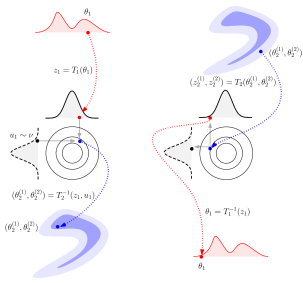
Formally, we first restrict the dimension of proposed auxiliary variables (if any) to , which is defined to be the dimension difference between and , i.e., . Then, assuming (a jump is proposed to a model of equal or higher dimension), the proposal is obtained via
| (5) | ||||
where each , is a diffeomorphism that both satisfies the pushforward-invariance condition
| (6) | ||||
and is volume-preserving (i.e., the absolute value of the Jacobian determinant is always equal to one). The default choice is to set each equal to the identity (resulting in the concatenation of the two inputs), but other choices are possible. For example, as is exchangeable, permutations are also suitable. Proposal moves to lower dimensions are similar to those in (5), but auxiliary variables of appropriate dimension are discarded as opposed to being drawn. The procedure of using our TRJ proposals within RJMCMC is given in Algorithm 1.
The following proposition provides a formal justification for the proposed approach, showing that when exact transports are used, (2) reduces to a form depending only on the marginal posterior model probabilities (i.e., there is a marginalizing effect).
Proposition 1.
Corollary 1.
Provided the conditions of Proposition 1 are satisfied, choosing such that
| (8) |
leads to a rejection-free proposal.
A natural choice when allowing global moves, i.e., for all that solves the above detailed balance condition (8), is simply to choose for all . Of course, in practice the marginal probabilities are typically unknown. However, the above observation is potentially instructive as to what a good choice may be if some approximation of model probabilities is available.
4 NUMERICAL EXPERIMENTS
For all experiments, we use masked autoregressive transforms with rational quadratic splines (RQMA) Durkan et al., (2020). Prior to the RQMA transforms, a fixed (i.e., non-trainable) element-wise standardization is applied, which we find has a positive effect on the speed and stability of training. We also consider simpler NFs in the form of affine transformations, which are constructed using the sample mean vector and Cholesky factorization of the sample covariance matrix of the training set (Affine NFs). We highlight that in general, the choice of normalizing flow family is essentially arbitrary. However, as the proposed TRJ approach requires that the flows be evaluated in both directions (i.e., both the original flow and its inverse are needed in order to transform both to and from the reference distribution), it is computationally convenient to employ flows that are analytically tractable in both directions (as is the case for RQMA and Affine flows). Such tractability does not hold for all flows. For example, Invertible Residual Networks (Behrmann et al.,, 2019) require numerical fixed-point iteration to evaluate in the inverse direction. In all experiments, flows are fit for each individual -conditional target using a set of training samples obtained via a pilot run of either MCMC, Sequential Monte Carlo samplers (Del Moral et al.,, 2006), or exact sampling. The performance of transdimensional proposals is benchmarked in two ways, discussed below.
Model Probability (Running Estimates).
One way to benchmark the performance of an RJMCMC chain is to visualize the running estimates of the marginal posterior probability of a given model as the RJMCMC chain progresses. On average, a chain that mixes more rapidly is expected to produce more accurate results with fewer iterations.
Bartolucci Bridge Estimator.
To assess the effect of different transdimensional proposals alone (as opposed to in combination with within-model moves), we employ the Bayes factor bridge-sampling estimator of Bartolucci et al., (2006, Eq.16). The estimator relies on constructing a Rao-Blackwellized bridge sampling approach. An advantage of the approach as originally introduced is that the estimators can be computed from stored values obtained from a standard RJMCMC run. Specifically, the Bayes factor (ratio of marginal likelihoods) is estimated via
| (9) |
where and are the number of proposed moves from model to , and from to , respectively in the run of the chain. The and terms are simply the acceptance probabilities corresponding to those proposals, respectively. Rather than use the output of an RJMCMC run, a straightforward alternative when one has samples from the individual conditionals (not necessarily obtained via RJMCMC) is the following. First, for each sample from each target, make one proposal of RJMCMC (inclusive of the random choice of model to jump to). Then, treat each of these as if they were a proposal obtained from a standard RJMCMC chain, used together to compute estimators of the form (9). In the special case when prior model probabilities are uniform, it is straightforward to convert estimators of Bayes factors to estimators of model probabilities (Bartolucci et al.,, 2006) via
| (10) |
for arbitrary . In the sequel, the combination of multiple estimators of the form (9) within (10) is referred to as the Bartolucci bridge estimator (BBE) of model probabilities. We expect the BBE to exhibit the lowest variance for the best across-model proposal type when computed using the same input set of samples from all models (as well as the same model jump probabilities ). When evaluating performance using the BBE, we generate an additional set of samples (for each model ) that are independent of the training samples. This set is referred to as the evaluation set. One proposal of RJMCMC is made using each of these evaluation samples to obtain the BBE (9) terms within the estimator of model probabilities (10).
4.1 Illustrative Example
To construct an illustrative example where the exact TMs are known, we use the (element-wise) inverse sinh-arcsinh (SAS) transformation (Jones and Pewsey,, 2009),
where , and . For an matrix , define a transform where
| (11) |
and . The probability density function for the transformed variable is
where . We consider a transdimensional target consisting of two models of dimension and . We assign a probability of for model with parameters and model probability of for with parameters . The target of interest for this example is
| (12) |
where
| (13) | ||||||
and is a lower-triangular matrix such that
By construction, for a reference distribution chosen to be a multidimensional standard Gaussian of appropriate dimension, an exact transport is given by the function
| (14) |
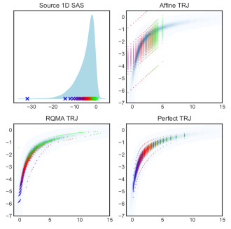
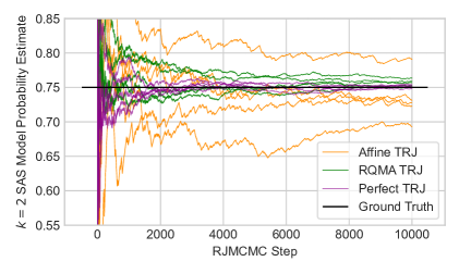
Note that the choice of , for , i.e., the mixture weights, correspond to a rejection-free proposal when the exact transports of the form in (14) are used. Both the affine and RQMA NF are trained on a set of samples obtained via exact simulation for each of the two targets. Figure 2 depicts a visualization of the proposal distributions (including those obtained using an exact transport map), and Figure 3 visualizes the running estimate of model probabilities for each proposal type, where is set to the mixture weights as above. On average, the accuracy of the running model probability estimates is best for the exact TM, followed by RQMC NF, which provides a better approximation of the exact TM compared to Affine.
4.2 Bayesian Factor Analysis Example
Here we consider the factor analysis (FA) model from Lopes and West, (2004). Factor analysis assumes the model where the covariance matrix takes the form , where is a positive diagonal matrix, is a lower-triangular matrix with a positive diagonal, is the number of factors, and the total number of parameters is . We model monthly exchange rates of six currencies relative to the British pound, spanning January 1975 to December 1986 West and Harrison, (1997) as 143 realizations, denoted as for . For this example, we are interested in or factors, yielding parameter spaces of dimensions 17 and 21 respectively. Following Lopes and West, (2004), for each with , , the priors are
| (15) | ||||
where denotes the positive half-normal distribution and the inverse gamma distribution. We are interested in the posterior of for or factors. Via Bayes’ Theorem, the posterior is
| (16) |
where . In this example, we compare TRJ proposals to the original RJMCMC proposal from Lopes and West, (2004). The form of the Lopes and West, (2004) RJMCMC proposal is an independence proposal trained on the conditional posterior of each model. Write and as the posterior mean and covariance matrix of , respectively. Defining , the independence proposal is , where for , , and where each is chosen to be an estimate of the marginal mode of for model obtained from the training samples.
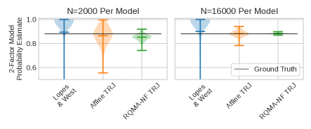
To obtain training and evaluation sets of samples from (16), we use the No-U-Turn Sampler (NUTS) Hoffman and Gelman, (2014) as implemented in PyMC Salvatier et al., (2016) for the three-factor model, and static temperature-annealed sequential Monte Carlo (SMC) Del Moral et al., (2006) for the two-factor model. The number of training and evaluation samples is kept equal, and the experiments consider both and for each. Ten pairs of training and evaluation sample sets are generated. Each evaluation process produces a single BBE estimate, and this is conducted 100 times per training/evaluation pair, yielding a total of BBE estimates.
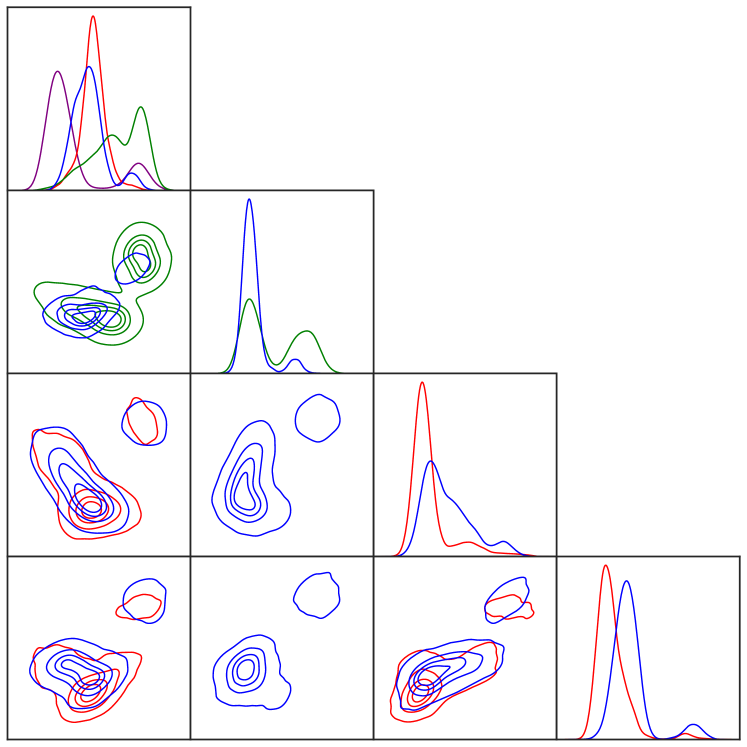
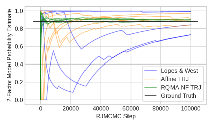
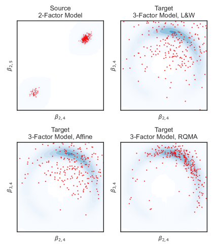
Figure 4 visualizes a comparison of the running estimate of the two-factor posterior model probability for RJMCMC chains that use the independence proposal and the RQMA-NF TRJ proposal against the ground truth value of as reported in Lopes and West, (2004). Each chain was run for steps with an RJMCMC proposal and a within-model random walk proposal used at each step in sequence. Figure 5 visualizes the variability of model probability estimates obtained from the BBE. Both figures demonstrate the superior performance of the TRJ sampler approach with RQMA flows compared to the standard approach of Lopes and West, (2004). Figure 6 visualizes the transdimensional proposals with respect to selected bivariate marginals.
5 CONDITIONAL TRANSPORT PROPOSALS
So far, we have introduced a proposition for rejection-free RJMCMC moves based on perfect TMs and model probabilities, and an approach to approximate both of the unknown quantities. However, there is one clear drawback to this approach: larger model spaces, such as those encountered in variable selection problems, would still require individual approximate TMs to be trained. This section explores how to overcome the above problem by modifying the sampling problem appropriately via a saturated space approach, so one can obtain the approximate TMs by training a single conditional NF (e.g., Winkler et al., (2019)). The general idea of the approach is that the model indicator is given as an input (context) to a function that outputs the parameters of a flow (or sequence thereof). Such an approach implicitly defines a family of flows across all models, yet only requires training once. The benefit is thus primarily computational. We employ the notation for the flow obtained by providing the conditional normalizing flow model with context .
The dimension-saturation approach, originally considered in Brooks et al., (2003), is an equivalent formulation of RJMCMC that involves an augmented target. Writing the maximum model dimension as (assumed to be finite) and recalling that , we define our augmented target to be
| (17) |
where , and “” identifies that the auxiliary variable is of dimension . In this setting, one can obtain approximate TMs by training a single conditional NF with the conditioning vector being the model index (further details are provided in the supplement). The associated proposals analogous to those in (5) are constructed as , where , and is simply concatenation. The above yields Algorithm 2.
5.1 Variable Selection in Robust Regression Example
Here, a variable selection example is provided as a proof of concept for the conditional transport approach just described. For this example, we seek a challenging Bayesian model choice problem where conventional methods do not perform well. The interest is in realizations of a random response variable , where for each , we have associated covariates where . Writing for the associated design matrix, our model is , where is the vector of unknown regression parameters and is the residual error term. We model as a vector of independently and identically distributed random variables, each distributed as a mixture of a standard normal variable and a zero-mean normal variable with variance . To ease the exposition, we adjust the notation slightly to accommodate the Bayesian variable selection literature. Let be an indicator vector where the th position of equals 1 if the variable is included in model and 0 otherwise — e.g., the model indexed by corresponds to the model with parameters . We consider a model space of cardinality of 4, composed of all models of the form where for . These models will include or exclude the parameters and jointly as commonly considered in group variable selection (e.g. Xu and Ghosh, (2015)). The prior distributions are specified as
| (18) | ||||
The target distribution is then the posterior distribution over the set of models and regression coefficients, obtained via Bayes’ Theorem.
The dataset for the example was simulated from the model , which has corresponding parameters . We simulated half of the observations of the response using and half using . This choice was made to induce further challenging multi-modal features in the resulting posterior. The elements of the matrix were simulated independently from a standard normal distribution, and the elements of the residual vector were simulated from a normal distribution with a mean of zero and a variance of 25. See the supplementary material for visualizations of the multimodal posterior behavior. The design of each proposal is as follows. The “standard” proposal adopts the independent auxiliary variable method of Brooks et al., (2003), which is equivalent to using the augmented target (17) where is the prior distribution for , i.e., . The standard proposals are deterministic in the sense that no auxiliary variables are drawn, but rather the block of parameters is reinstated to its previous value when . The TRJ affine and RQMA-NF proposals apply Algorithm 1 with approximate affine, and RQMA-NF TMs respectively trained on samples from the conditional target distributions. The CTRJ proposal adopts the augmented target (17) where is set to the reference univariate density as described in Section 5, and proceeds as per Algorithm 2. The empirical performance of each proposal is examined for training and evaluation sets via the BBE. The number of training and evaluation samples was kept the same, and we considered both and sampled from a single SMC run. The process of training the flow and estimation of model probability via BBE was repeated eighty times.
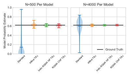
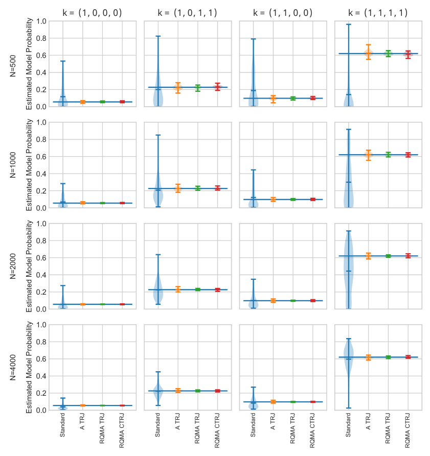
Figure 7 visualizes the variability of the model probability estimate using the same approach as in Section 4.2. The figure shows the vastly superior accuracy and variability of model probability estimates using the TRJ proposals relative to the independent auxiliary method. The performance of the conditional RQMA flow appears similar to that of the individual RQMA and affine flows but only requires fitting a single conditional flow as opposed to a flow per model.
6 DISCUSSION
The work introduces a method to design across-model RJMCMC proposals using ideas from measure transport. The approach was shown to have desirable properties in the case where exact TMs are used, while still providing good performance in the case where the TMs are approximate. Although some form of initial effort to obtain samples from each conditional target is somewhat common when calibrating proposals (e.g., as in Lopes and West, (2004); Hastie, (2005)), this is still a weakness of TRJ proposals, along with the computational effort required to train the approximate transport maps. The use of conditional NFs may mitigate the latter somewhat, but a promising avenue for future research would be some form of amortized approach in model spaces where there is some shared structure (and thus perhaps samples from only some models would suffice). Moreover, the effort may be justified in settings where likelihoods are particularly expensive, gradient-based methods are unavailable (e.g., implicit models), or by and large the gain in performance appropriately justifies the effort in obtaining the approximate TMs. Finally, while we mainly repurposed the BBE to benchmark cross-model proposal quality, the results seem promising, and it may be interesting to explore its use in lieu of standard RJMCMC if efforts to obtain approximate TMs have already occurred.
Acknowledgements
Christopher Drovandi acknowledges support from an Australian Research Council Discovery Project (DP200102101), which Laurence Davies was also partially supported by.
References
- Al-Awadhi et al., (2004) Al-Awadhi, F., Hurn, M., and Jennison, C. (2004). Improving the acceptance rate of reversible jump MCMC proposals. Statistics & Probability Letters, 69(2):189–198.
- Arbel et al., (2021) Arbel, M., Matthews, A., and Doucet, A. (2021). Annealed flow transport Monte Carlo. In International Conference on Machine Learning, pages 318–330. PMLR.
- Bartolucci et al., (2006) Bartolucci, F., Scaccia, L., and Mira, A. (2006). Efficient Bayes factor estimation from the reversible jump output. Biometrika, 93(1):41–52.
- Behrmann et al., (2019) Behrmann, J., Grathwohl, W., Chen, R. T. Q., Duvenaud, D., and Jacobsen, J.-H. (2019). Invertible residual networks. In Chaudhuri, K. and Salakhutdinov, R., editors, Proceedings of the 36th International Conference on Machine Learning, volume 97 of Proceedings of Machine Learning Research, pages 573–582. PMLR.
- Brooks et al., (2003) Brooks, S. P., Giudici, P., and Roberts, G. O. (2003). Efficient construction of reversible jump Markov chain Monte Carlo proposal distributions. Journal of the Royal Statistical Society: Series B (Statistical Methodology), 65(1):3–39.
- Del Moral et al., (2006) Del Moral, P., Doucet, A., and Jasra, A. (2006). Sequential Monte Carlo samplers. Journal of the Royal Statistical Society: Series B (Statistical Methodology), 68(3):411–436.
- Durkan et al., (2019) Durkan, C., Bekasov, A., Murray, I., and Papamakarios, G. (2019). Neural Spline Flows. In Advances in Neural Information Processing Systems, volume 32. Curran Associates, Inc.
- Durkan et al., (2020) Durkan, C., Bekasov, A., Murray, I., and Papamakarios, G. (2020). nflows: normalizing flows in PyTorch. https://zenodo.org/record/4296287.
- Fan et al., (2008) Fan, Y., Peters, G. W., and Sisson, S. A. (2008). Automating and evaluating reversible jump MCMC proposal distributions. Statistics and Computing, 19(4):409.
- Farr et al., (2015) Farr, W. M., Mandel, I., and Stevens, D. (2015). An efficient interpolation technique for jump proposals in reversible-jump Markov chain Monte Carlo calculations. Royal Society Open Science, 2(6):150030.
- Gabrié et al., (2022) Gabrié, M., Rotskoff, G. M., and Vanden-Eijnden, E. (2022). Adaptive Monte Carlo augmented with normalizing flows. Proceedings of the National Academy of Sciences, 119(10):e2109420119.
- Gagnon, (2021) Gagnon, P. (2021). Informed reversible jump algorithms. Electronic Journal of Statistics, 15(2):3951–3995.
- Green, (1995) Green, P. J. (1995). Reversible jump Markov chain Monte Carlo computation and Bayesian model determination. Biometrika, 82(4):711–732.
- Green and Mira, (2001) Green, P. J. and Mira, A. (2001). Delayed rejection in reversible jump Metropolis-Hastings. Biometrika, 88(4):1035–1053.
- Hastie, (2005) Hastie, D. (2005). Towards Automatic Reversible Jump Markov Chain Monte Carlo. PhD thesis, University of Bristol.
- Hastings, (1970) Hastings, W. K. (1970). Monte Carlo sampling methods using Markov chains and their applications. Biometrika, 57(1):97–109.
- Hoffman et al., (2018) Hoffman, M., Sountsov, P., Dillon, J. V., Langmore, I., Tran, D., and Vasudevan, S. (2018). NeuTra-lizing bad geometry in Hamiltonian Monte Carlo using neural transport. In 1st Symposium on Advances in Approximate Bayesian Inference.
- Hoffman and Gelman, (2014) Hoffman, M. D. and Gelman, A. (2014). The No-U-turn sampler: adaptively setting path lengths in Hamiltonian Monte Carlo. The Journal of Machine Learning Research, 15(1):1593–1623.
- Jones and Pewsey, (2009) Jones, M. C. and Pewsey, A. (2009). Sinh-arcsinh distributions. Biometrika, 96(4):761–780.
- Karagiannis and Andrieu, (2013) Karagiannis, G. and Andrieu, C. (2013). Annealed importance sampling reversible jump MCMC algorithms. Journal of Computational and Graphical Statistics, 22(3):623–648.
- Lopes and West, (2004) Lopes, H. F. and West, M. (2004). Bayesian model assessment in factor analysis. Statistica Sinica, 14(1):41–67.
- Papamakarios et al., (2021) Papamakarios, G., Nalisnick, E. T., Rezende, D. J., Mohamed, S., and Lakshminarayanan, B. (2021). Normalizing flows for probabilistic modeling and inference. Journal of Machine Learning Research, 22(57):1–64.
- Parno and Marzouk, (2018) Parno, M. D. and Marzouk, Y. M. (2018). Transport map accelerated Markov chain Monte Carlo. SIAM/ASA Journal on Uncertainty Quantification, 6(2):645–682.
- Salvatier et al., (2016) Salvatier, J., Wiecki, T. V., and Fonnesbeck, C. (2016). Probabilistic programming in Python using PyMC3. PeerJ Computer Science, 2:e55.
- South et al., (2019) South, L. F., Pettitt, A. N., and Drovandi, C. (2019). Sequential Monte Carlo samplers with independent Markov chain Monte Carlo proposals. Bayesian Analysis, 14(3):753–776.
- West and Harrison, (1997) West, M. and Harrison, J. (1997). Bayesian forecasting and dynamic models. Springer series in statistics. Springer, New York, 2nd ed edition.
- Winkler et al., (2019) Winkler, C., Worrall, D., Hoogeboom, E., and Welling, M. (2019). Learning likelihoods with conditional normalizing flows. arXiv preprint arXiv:1912.00042.
- Xu and Ghosh, (2015) Xu, X. and Ghosh, M. (2015). Bayesian variable selection and estimation for group lasso. Bayesian Analysis, 10(4):909–936.
- Zanella, (2020) Zanella, G. (2020). Informed proposals for local MCMC in discrete spaces. Journal of the American Statistical Association, 115(530):852–865.
SUPPLEMENTARY MATERIAL
Appendix A PROOF OF PROPOSITION 1
Proof.
Here, we employ the shorthand notation and for measure and probability density functions, respectively. For a diffeomorphism , auxiliary variables , of respective dimensions and , if the dimension matching requirement is satisfied, then the standard choice (Green,, 1995) for the acceptance probability that satisfies detailed balance is
| (19) |
First, consider the case that . The proposed move from index to is
| (20) |
In this setting, we have , , and . Note that (i.e., an “empty” distribution), so . Further, the dimension-matching requirement reduces to . Using the properties that and , along with the assumption that is a volume-preserving map, i.e., , we have that
| (21) |
Making the above substitutions into (19), and employing the conditional factorization identity to both and yields
| (22) |
Hence, showing that the bracketed term above must always be equal to one establishes the desired result. To accomplish this, we make use of several identities. First, note that by hypothesis, and are diffeomorphic and satisfy and . Thus, by the standard change of variables theorem, we obtain the identities
| (23) | ||||
Next, by hypothesis , and since is a volume-preserving diffeomorphism we obtain
| (24) |
Finally, observe
| (25) |
where the final equality above uses associativity of function composition. Using the above identities, and that , we obtain
and the result is established for the stated case. The result is established for the case by repeating the above argument but setting because in that case. Similarly, for the case where , repeat the above argument by applying the reverse move (replacing with ), and using . ∎
Appendix B NORMALIZING FLOW CONFIGURATIONS
This section gives details regarding the flows used in the experiments. Write to denote the sigmoid function (applied element-wise). Define
| (26) |
The flow-based models used are of the form , where is the composition of three (3) masked autoregressive rational quadratic spline transforms, implemented in the Python package nflows. Parameters used for each of the three transforms were bins (corresponding to “knot” points), the autoregressive neural networks used in each transform had two hidden layers, each with hidden features. A Stochastic Gradient Descent (SGD) algorithm is used to train the parameters of the sequence of transforms . The transform is fixed at the beginning of training and remains so during training, with the values of and taken to be the marginal means and reciprocal standard deviations of the data (samples), respectively, from a given . It is beneficial to fix as described above as it essentially standardizes the data prior to model training.
B.1 Conditional Normalizing Flow
The conditional approach uses the conditional transform . In the previous equation, is now a conditional normalizing flow model that, given as input a context (conditioning) variable , outputs a flow of the same form as in the non-conditional case. Additionally, the CNF base distribution is now a conditional base — an independent Gaussian whose mean and scale parameters are determined via a context (implemented as ConditionalDiagonalNormal in nflows). Finally, is a conditional standardization that takes into account the known distribution of the auxiliary variables as well as when they feature for different models. Note that under the augmented target distribution, conditional on , is distributed according to the conditional target , and the auxiliary variables are distributed according to . Rather than simply standardize the auxilliary variables (which are known to be marginally distributed according to ) for each model, it is often straightforward to apply a perfect Gaussianizing transform. Write for the cumulative density function (cdf) of the reference distribution , and for the inverse cdf of the univariate standard normal distribution (i.e., the probit function). The generalization of the standardizing transform to the saturated state space (defined for output ) is then
| (27) |
Similar to the unconditional case, the vectors and are fixed to be the reciprocal standard deviation and mean vectors of the data (samples) from each . Optionally, one can set and for all using the same quantities obtained from pooling the samples (this is the approach implemented). In the considered example, the reference distribution was taken to be a standard Gaussian, and thus the second case above reduces simply to returning . We highlight that the check for which case to apply in the function above is implemented via a masking function that, for input , returns one if the condition is satisfied, and zero otherwise.
Appendix C BLOCK VARIABLE SELECTION EXAMPLE
Figure 8 depicts the distributions for each conditional target in the example. Note that each is multi-modal. However, there are overlaps in some regions of high probability mass, which could possibly assist the performance of the CTRJ proposal. Figure 9 is an extended version of Figure 7 in the paper, showing results of the Bartolucci estimator across varying number of samples for each of the four estimated model probabilities.
