Coupling chemotaxis and growth poromechanics
for the modelling of feather primordia patterning

Nicolás A. Barnafi Department of Mathematics, Università di Pavia, Via Ferrata 1, 27100 Pavia, Italy. E-mail: nicolas.barnafi@unipv.it    Luis Miguel De Oliveira Vilaca Laboratory of Artificial & Natural Evolution (LANE), Department of Genetics and Evolution, University of Geneva, 4 Boulevard d’Yvoy, 1205 Geneva, Switzerland; and SIB Swiss Institute of Bioinformatics, Geneva, Switzerland. E-mail: LuisMiguel.DeOliveiraVilaca@unige.ch, Michel.Milinkovitch@unige.ch    Michel C. Milinkovitch22footnotemark: 2    Ricardo Ruiz-Baier School of Mathematics, Monash University, 9 Rainforest Walk, Melbourne 3800 VIC, Australia; and Universidad Adventista de Chile, Casilla 7-D, Chillán, Chile. E-mail: ricardo.ruizbaier@monash.edu
Abstract

We propose a new mathematical model for the interaction of skin cell populations with fibroblast growth factor and bone morphogenetic protein, occurring within deformable porous media. The equations for feather primordia pattering are based on the work by K.J. Painter et al. [J. Theoret. Biol., 437 (2018) 225–238]. We perform a linear stability analysis to identify relevant parameters in the coupling mechanisms, focusing in the regime of infinitesimal strains. We also extend the model to the case of nonlinear poroelasticity and include solid growth by means of Lee decompositions of the deformation gradient. We present a few illustrative computational examples in 2D and 3D, and briefly discuss the design of tailored efficient solvers.

1 Introduction

Chemotaxis models [24] describe the directed movement of cells in response to chemicals (attractants or repellents), and can predict the formation of clustered structures. This process has been observed in a variety of embryogenesis processes, such as gastrulation [48] and feather development [27]. In the latter, we refer to the buds that then give origin to feathers as primordia, and their origin has been modelled through Keller–Segel type chemotaxis models considering fibroblast growth factor (FGF) and bone morphogenic protein (BMP) [33, 35, 36].

Poroelasticity is a mixture model in which a solid phase coexists with (at least) one fluid phase [12]. Biological organs and tissues are naturally porous at the tissue level, as they are composed, for example, of both muscle and blood. This phase separation persists even up to the cellular level, as there is the cytoskeleton and the cytoplasm. For this reason, poroelastic models have become very pervasive in the modelling of soft living tissue, such as in oedema formation [3, 28], cardiac perfusion [47, 2], lung characterisation [7], and brain injury [46].

In the context of biologically-oriented problems, experiments have shown that the rheology of cytoplasm within living cells exhibits a poroelastic behaviour [31], and in turn, the composition of cells and the extracellular matrix constitutes an overall poromechanical system. The presence of chemical solutes locally modifies morphoelastic properties and these processes can be homogenised to obtain macroscopic models of poroelasticity coupled with advection-reaction-diffusion equations (see e.g. [11, 37]). With this biological basis, the scope of our work is twofold: on one hand, we extend the existing pattern formation models for primordia by considering their interaction with the intracellular space in the outset of growth. On the other hand, we perform a thorough stability analysis to understand the coupling mechanisms in the model and to investigate the conditions that give rise to pattern formation.

We have structured the remainder of this paper in the following manner. Section 2 describes the coupled model for poro-mechano-chemical interactions, restricting the presentation to the regime of linear poroelasticity. We give an adimensional form of the governing equations, making precise boundary and initial conditions. In Section  3 we perform a linear stability analysis addressing pattern formation according to Turing instabilities. We separate the discussion in some relevant cases and derive and portray patterning spaces. Section 4 is devoted to extending the model to the case of nonlinear (finite-strain) poroelasticity and material growth, stating also the coupling with chemotaxis in the undeformed configuration. Some numerical examples are given in Section 5 and we close with a summary and discussion of model extensions in Section 6.

2 A coupled model of linear poroelasticity and chemotaxis

Let us consider a piece of soft material as a porous medium in dsuperscript𝑑\mathbb{R}^{d}, d=2,3𝑑23d=2,3, composed by a mixture of incompressible grains and interstitial fluid, whose description can be placed in the context of the classical Biot consolidation problem (see e.g. [42]). In the absence of gravitational forces, of body loads, and of mass sources or sinks, we seek for each time t(0,tfinal]𝑡0subscript𝑡finalt\in(0,t_{\mathrm{final}}], the displacement of the porous skeleton, 𝒖(t):Ωd:𝒖𝑡Ωsuperscript𝑑\boldsymbol{u}(t):\Omega\to\mathbb{R}^{d}, and the pore pressure of the fluid, p(t):Ω:𝑝𝑡Ωp(t):\Omega\to\mathbb{R}, such that

t(C0p+αBWdiv𝒖)1ηdiv{κp}subscript𝑡subscript𝐶0𝑝subscript𝛼𝐵𝑊div𝒖1𝜂div𝜅𝑝\displaystyle\partial_{t}\bigl{(}C_{0}p+\alpha_{BW}\mathop{\mathrm{div}}\nolimits\boldsymbol{u}\bigr{)}-\frac{1}{\eta}\mathop{\mathrm{div}}\nolimits\{\kappa\nabla p\} =0absent0\displaystyle=0 in Ω×(0,tfinal],in Ω×(0,tfinal]\displaystyle\text{in $\Omega\times(0,t_{\mathrm{final}}]$}, (2.1a)
𝝈𝝈\displaystyle\boldsymbol{\sigma} =𝝈poroelast+𝝈actabsentsubscript𝝈poroelastsubscript𝝈act\displaystyle=\boldsymbol{\sigma}_{\text{poroelast}}+\boldsymbol{\sigma}_{\text{act}} in Ω×(0,tfinal],in Ω×(0,tfinal]\displaystyle\text{in $\Omega\times(0,t_{\mathrm{final}}]$}, (2.1b)
ρtt𝒖𝐝𝐢𝐯𝝈𝜌subscript𝑡𝑡𝒖𝐝𝐢𝐯𝝈\displaystyle\rho\partial_{tt}\boldsymbol{u}-\mathop{\mathbf{div}}\nolimits\boldsymbol{\sigma} =𝟎absent0\displaystyle=\boldsymbol{0} in Ω×(0,tfinal],in Ω×(0,tfinal]\displaystyle\text{in $\Omega\times(0,t_{\mathrm{final}}]$}, (2.1c)

where κ(𝒙)𝜅𝒙\kappa(\boldsymbol{x}) is the hydraulic conductivity of the porous medium, ρ𝜌\rho is the density of the solid material, η𝜂\eta is the constant viscosity of the interstitial fluid, C0subscript𝐶0C_{0} is the constrained specific storage coefficient, αBWsubscript𝛼𝐵𝑊\alpha_{BW} is the Biot-Willis consolidation parameter, In (2.1b) we are supposing that the poromechanical deformations are also actively influenced by microscopic tension generation. A very simple description is given in terms of active stresses: we assume that the total Cauchy stress contains a passive and an active component, where

𝝈poroelast=λ(div𝒖)𝐈+2μ𝜺(𝒖)p𝐈,subscript𝝈poroelast𝜆div𝒖𝐈2𝜇𝜺𝒖𝑝𝐈\boldsymbol{\sigma}_{\text{poroelast}}=\lambda(\mathop{\mathrm{div}}\nolimits\boldsymbol{u})\mathbf{I}+2\mu\boldsymbol{\varepsilon}(\boldsymbol{u})-p\mathbf{I}, (2.2)

and 𝝈actsubscript𝝈act\boldsymbol{\sigma}_{\text{act}} is specified in (2.5), below. The tensor 𝜺(𝒖)=12(𝒖+𝒖)𝜺𝒖12bold-∇𝒖bold-∇superscript𝒖\boldsymbol{\varepsilon}(\boldsymbol{u})=\frac{1}{2}(\boldsymbol{\nabla}\boldsymbol{u}+\boldsymbol{\nabla}\boldsymbol{u}^{\intercal}) is that of infinitesimal strains, 𝐈𝐈\mathbf{I} denotes the second-order identity tensor, and μ,λ𝜇𝜆\mu,\lambda are the Lamé constants (shear and dilation moduli) of the solid structure. Equations (2.1a)-(2.1c) represent the conservation of mass, the constitutive relation, and the conservation of linear momentum, respectively.

In addition, let us consider a modified Patlak–Keller–Segel model for the distribution of chemotactic cell populations of mesenchymal cells, m𝑚m, epithelium activation state, e𝑒e, fibroblast growth factor (FGF), f𝑓f, and bone morphogenetic protein (BMP), b𝑏b. The base-line model has been developed in [36] and (after being properly modified to account for the motion of the underlying deformable porous media) it can be summarised as follows

tm+t𝒖mdiv(Dmmαmexp(γm)f)subscript𝑡𝑚subscript𝑡𝒖𝑚divsubscript𝐷𝑚𝑚𝛼𝑚𝛾𝑚𝑓\displaystyle\partial_{t}m+\partial_{t}\boldsymbol{u}\cdot\nabla m-\mathop{\mathrm{div}}\nolimits\bigl{(}D_{m}\nabla m-\alpha m\exp(-\gamma m)\nabla f\bigr{)} =0absent0\displaystyle=0 in Ω×(0,tfinal],in Ω0subscript𝑡final\displaystyle\text{in }\Omega\times(0,t_{\mathrm{final}}], (2.3a)
te[κ1w(𝒙,t)h1(m)+κ2h2(m)](1e)+[1h1(m)](κ3+κ4b)esubscript𝑡𝑒delimited-[]subscript𝜅1𝑤𝒙𝑡subscript1𝑚subscript𝜅2subscript2𝑚1𝑒delimited-[]1subscript1𝑚subscript𝜅3subscript𝜅4𝑏𝑒\displaystyle\partial_{t}e-[\kappa_{1}w(\boldsymbol{x},t)h_{1}(m)+\kappa_{2}h_{2}(m)](1-e)+[1-h_{1}(m)](\kappa_{3}+\kappa_{4}b)e =0absent0\displaystyle=0 in Ω×(0,tfinal],in Ω0subscript𝑡final\displaystyle\text{in }\Omega\times(0,t_{\mathrm{final}}], (2.3b)
tf+t𝒖fdiv(Dff)κFe+δFf+ξfdiv𝒖subscript𝑡𝑓subscript𝑡𝒖𝑓divsubscript𝐷𝑓𝑓subscript𝜅𝐹𝑒subscript𝛿𝐹𝑓subscript𝜉𝑓div𝒖\displaystyle\partial_{t}f+\partial_{t}\boldsymbol{u}\cdot\nabla f-\mathop{\mathrm{div}}\nolimits(D_{f}\,\nabla f)-\kappa_{F}e+\delta_{F}f+\xi_{f}\mathop{\mathrm{div}}\nolimits\boldsymbol{u} =0absent0\displaystyle=0 in Ω×(0,tfinal],in Ω0subscript𝑡final\displaystyle\text{in }\Omega\times(0,t_{\mathrm{final}}], (2.3c)
tb+t𝒖bdiv(Dbb)κBh3(m)m+δBbsubscript𝑡𝑏subscript𝑡𝒖𝑏divsubscript𝐷𝑏𝑏subscript𝜅𝐵subscript3𝑚𝑚subscript𝛿𝐵𝑏\displaystyle\partial_{t}b+\partial_{t}\boldsymbol{u}\cdot\nabla b-\mathop{\mathrm{div}}\nolimits(D_{b}\,\nabla b)-\kappa_{B}h_{3}(m)m+\delta_{B}b =0absent0\displaystyle=0 in Ω×(0,tfinal],in Ω0subscript𝑡final\displaystyle\text{in }\Omega\times(0,t_{\mathrm{final}}], (2.3d)

where Dm,Df,Dbsubscript𝐷𝑚subscript𝐷𝑓subscript𝐷𝑏D_{m},D_{f},D_{b} are positive definite diffusion matrices, and the spatio-temporal and nonlinear coefficients (in this case, the priming wave responsible for the generation of spatial patterns and the degree of clustering of mesenchymal cells, respectively) are defined as

w(𝒙,t)=ω12{1+tanh(ω2[tx2/ω3])},hi(m)=mPi[KiPi+mPi]1,formulae-sequence𝑤𝒙𝑡subscript𝜔121subscript𝜔2delimited-[]𝑡subscript𝑥2subscript𝜔3subscript𝑖𝑚superscript𝑚subscript𝑃𝑖superscriptdelimited-[]superscriptsubscript𝐾𝑖subscript𝑃𝑖superscript𝑚subscript𝑃𝑖1w(\boldsymbol{x},t)=\frac{\omega_{1}}{2}\{1+\tanh(\omega_{2}[t-x_{2}/\omega_{3}])\},\qquad h_{i}(m)=m^{P_{i}}[K_{i}^{P_{i}}+m^{P_{i}}]^{-1}, (2.4)

where κi,ωi,Pi,γ,δi,ξfsubscript𝜅𝑖subscript𝜔𝑖subscript𝑃𝑖𝛾subscript𝛿𝑖subscript𝜉𝑓\kappa_{i},\omega_{i},P_{i},\gamma,\delta_{i},\xi_{f} are positive model constants. Note that the mechano-chemical feedback (the process where mechanical forces modify the reaction-diffusion effects) is here assumed only through an additional reaction term in the FGF equation (2.3c), depending linearly on volume change. Since ξf>0subscript𝜉𝑓0\xi_{f}>0, this contribution acts as a local sink of FGF during dilation.

On the other hand, we assume that the active stress component acts isotropically on the medium (see e.g. [22]), and it depends nonlinearly on the concentration of mesenchymal cells, as proposed for instance in [34]

𝝈act=(λ+2μ3)τm1+ζm2𝐈,subscript𝝈act𝜆2𝜇3𝜏𝑚1𝜁superscript𝑚2𝐈\boldsymbol{\sigma}_{\text{act}}=\biggl{(}\lambda+\frac{2\mu}{3}\biggr{)}\frac{\tau m}{1+\zeta m^{2}}\mathbf{I}, (2.5)

with τ𝜏\tau a model constant to be specified later on, which can be positive (implying that the function modifies the motion of the medium as a local dilation) or negative (isotropically distributed compression).

In order to reduce the number of model parameters, we focus on a dimensionless counterpart of systems (2.1a)-(2.1c) and (2.3a)-(2.3d), which can be derived using the following transformation, suggested in [36]

m=mγ,e=e,f=κFfδB,b=κBbγ,formulae-sequence𝑚superscript𝑚𝛾formulae-sequence𝑒superscript𝑒formulae-sequence𝑓subscript𝜅𝐹superscript𝑓subscript𝛿𝐵𝑏subscript𝜅𝐵superscript𝑏𝛾\displaystyle m=\frac{m^{*}}{\gamma},\quad e=e^{*},\quad f=\frac{\kappa_{F}f^{*}}{\delta_{B}},\quad b=\frac{\kappa_{B}b^{*}}{\gamma},
𝒖=DbδB𝒖,p=p,t=tδB,𝒙=DbδB𝒙,formulae-sequence𝒖subscript𝐷𝑏subscript𝛿𝐵superscript𝒖formulae-sequence𝑝superscript𝑝formulae-sequence𝑡superscript𝑡subscript𝛿𝐵𝒙subscript𝐷𝑏subscript𝛿𝐵superscript𝒙\displaystyle\boldsymbol{u}=\sqrt{\frac{D_{b}}{\delta_{B}}}\boldsymbol{u}^{*},\quad p=p^{*},\quad t=\frac{t^{*}}{\delta_{B}},\quad\boldsymbol{x}=\sqrt{\frac{D_{b}}{\delta_{B}}}\boldsymbol{x}^{*},

where hereafter the stars are dropped for notational convenience. The adimensional coupled system is then equipped with appropriate initial data at rest

m(0)=m0,e(0)=e0=κ1w(𝒙,0)h1(m0)+κ2h2(m0)κ1w(𝒙,0)h1(m0)+κ2h2(m0)+[1h1(m0)](κ3+κ4b),formulae-sequence𝑚0subscript𝑚0𝑒0subscript𝑒0subscript𝜅1𝑤𝒙0subscript1subscript𝑚0subscript𝜅2subscript2subscript𝑚0subscript𝜅1𝑤𝒙0subscript1subscript𝑚0subscript𝜅2subscript2subscript𝑚0delimited-[]1subscript1subscript𝑚0subscript𝜅3subscript𝜅4𝑏\displaystyle m(0)=m_{0},\quad e(0)=e_{0}=\frac{\kappa_{1}w(\boldsymbol{x},0)h_{1}(m_{0})+\kappa_{2}h_{2}(m_{0})}{\kappa_{1}w(\boldsymbol{x},0)h_{1}(m_{0})+\kappa_{2}h_{2}(m_{0})+[1-h_{1}(m_{0})](\kappa_{3}+\kappa_{4}b)},
f(0)=e0δF,b(0)=h3(m0)m0,𝒖(0)=𝟎,t𝒖(0)=𝟎,p(0)=0,formulae-sequence𝑓0subscript𝑒0subscript𝛿𝐹formulae-sequence𝑏0subscript3subscript𝑚0subscript𝑚0formulae-sequence𝒖00formulae-sequencesubscript𝑡𝒖00𝑝00\displaystyle f(0)=\frac{e_{0}}{\delta_{F}},\quad b(0)=h_{3}(m_{0})m_{0},\quad\boldsymbol{u}(0)=\boldsymbol{0},\quad\partial_{t}\boldsymbol{u}(0)=\boldsymbol{0},\quad p(0)=0, (2.6)

defined in ΩΩ\Omega; and boundary conditions in the following manner

{Dmmαmexp(γm)f}𝒏=Dff𝒏=b𝒏subscript𝐷𝑚𝑚𝛼𝑚𝛾𝑚𝑓𝒏subscript𝐷𝑓𝑓𝒏𝑏𝒏\displaystyle\{D_{m}\,\nabla m-\alpha m\exp(-\gamma m)\nabla f\}\cdot\boldsymbol{n}=D_{f}\,\nabla f\cdot\boldsymbol{n}=\nabla b\cdot\boldsymbol{n} =0absent0\displaystyle=0 on Ω×(0,tfinal],on Ω×(0,tfinal]\displaystyle\text{on $\partial\Omega\times(0,t_{\text{final}}]$}, (2.7a)
𝒖=𝒖Γandκηp𝒏𝒖subscript𝒖Γand𝜅𝜂𝑝𝒏\displaystyle\boldsymbol{u}=\boldsymbol{u}_{\Gamma}\quad\text{and}\quad\frac{\kappa}{\eta}\nabla p\cdot\boldsymbol{n} =0absent0\displaystyle=0 on Γ×(0,tfinal],on Γ×(0,tfinal]\displaystyle\text{on $\Gamma\times(0,t_{\text{final}}]$}, (2.7b)
𝝈𝒏=𝒕andp𝝈𝒏𝒕and𝑝\displaystyle\boldsymbol{\sigma}\boldsymbol{n}=\boldsymbol{t}\quad\text{and}\quad p =p0absentsubscript𝑝0\displaystyle=p_{0} on Σ×(0,tfinal],on Σ×(0,tfinal]\displaystyle\text{on $\Sigma\times(0,t_{\text{final}}]$}, (2.7c)

where 𝒏𝒏\boldsymbol{n} denotes the outward unit normal on the boundary, and Ω=ΓΣΩΓΣ\partial\Omega=\Gamma\cup\Sigma is disjointly split into ΓΓ\Gamma and ΣΣ\Sigma where we prescribe clamped boundaries and zero fluid normal fluxes; and a given traction 𝒕𝒕\boldsymbol{t} together with constant fluid pressure p0subscript𝑝0p_{0}, respectively.

3 Linear stability analysis and dispersion relation

3.1 Preliminaries.

We proceed to derive a linear stability analysis for the coupled problem (2.1a)-(2.5). As usual the analysis is performed on an infinite domain in dsuperscript𝑑\mathbb{R}^{d}, with d=2,3𝑑23d=2,3. The first step consists in linearising the poro-mechano-chemical system around a steady state, defined in (2). The linearised dimensionless equations are given by

t(C0p+αBWdiv𝒖)1ηdiv{κp}=0,ρtt𝒖𝐝𝐢𝐯(𝝈poroelast+𝝈actlin)=𝟎,tmdiv{Dmmαm0em0f}=0,teAm(m0,e0)m+Ae(m0,b0)e+Ab(m0,e0)b=0,tfdiv{Dff}e+δFf+ξfdiv𝒖=0,tbΔbH3(m0)m+δBb=0,formulae-sequencesubscript𝑡subscript𝐶0𝑝subscript𝛼𝐵𝑊div𝒖1𝜂div𝜅𝑝0formulae-sequence𝜌subscript𝑡𝑡𝒖𝐝𝐢𝐯subscript𝝈poroelastsuperscriptsubscript𝝈actlin0formulae-sequencesubscript𝑡𝑚divsubscript𝐷𝑚𝑚𝛼subscript𝑚0superscriptesubscript𝑚0𝑓0formulae-sequencesubscript𝑡𝑒subscript𝐴𝑚subscript𝑚0subscript𝑒0𝑚subscript𝐴𝑒subscript𝑚0subscript𝑏0𝑒subscript𝐴𝑏subscript𝑚0subscript𝑒0𝑏0formulae-sequencesubscript𝑡𝑓divsubscript𝐷𝑓𝑓𝑒subscript𝛿𝐹𝑓subscript𝜉𝑓div𝒖0subscript𝑡𝑏Δ𝑏subscript𝐻3subscript𝑚0𝑚subscript𝛿𝐵𝑏0\begin{split}\partial_{t}\bigl{(}C_{0}p+\alpha_{BW}\mathop{\mathrm{div}}\nolimits\boldsymbol{u}\bigr{)}-\frac{1}{\eta}\mathop{\mathrm{div}}\nolimits\{\kappa\nabla p\}&=0,\\ \rho\partial_{tt}\boldsymbol{u}-\mathop{\mathbf{div}}\nolimits\bigl{(}\boldsymbol{\sigma}_{\text{poroelast}}+\boldsymbol{\sigma}_{\text{act}}^{\text{lin}}\bigr{)}&=\boldsymbol{0},\\ \partial_{t}m-\mathop{\mathrm{div}}\nolimits\{D_{m}\nabla m-\alpha m_{0}\mathrm{e}^{-m_{0}}\nabla f\}&=0,\\ \partial_{t}e-A_{m}(m_{0},e_{0})m+A_{e}(m_{0},b_{0})e+A_{b}(m_{0},e_{0})b&=0,\\ \partial_{t}f-\mathop{\mathrm{div}}\nolimits\{D_{f}\,\nabla f\}-e+\delta_{F}f+\xi_{f}\mathop{\mathrm{div}}\nolimits\boldsymbol{u}&=0,\\ \partial_{t}b-\Delta b-H_{3}(m_{0})m+\delta_{B}b&=0,\end{split} (3.1)

where

𝝈actlin=((λ+2μ3)τ1ζm02(1+ζm02)2)m𝐈,superscriptsubscript𝝈actlin𝜆2𝜇3𝜏1𝜁superscriptsubscript𝑚02superscript1𝜁superscriptsubscript𝑚022𝑚𝐈\boldsymbol{\sigma}_{\text{act}}^{\text{lin}}=\left(\left(\lambda+\frac{2\mu}{3}\right)\tau\frac{1-\zeta m_{0}^{2}}{\left(1+\zeta m_{0}^{2}\right)^{2}}\right)m\mathbf{I},

and Amsubscript𝐴𝑚A_{m}, Aesubscript𝐴𝑒A_{e}, Absubscript𝐴𝑏A_{b}, H3subscript𝐻3H_{3} are functions of the steady state values, which will be made precise in Definition 3.1, below. We look then for solutions of the form 𝒖,p,m,e,f,bei𝒌𝒙+ϕtproportional-to𝒖𝑝𝑚𝑒𝑓𝑏superscript𝑒i𝒌𝒙italic-ϕ𝑡\boldsymbol{u},p,m,e,f,b\propto e^{\mathrm{i}\boldsymbol{k}\cdot\boldsymbol{x}+\phi t}, where 𝒌𝒌\boldsymbol{k} is the wave vector (a measure of spatial structure) and ϕitalic-ϕ\phi is the linear growth factor. By substituting this ansatz on the system (3.1), we get a system of linear equations for the vector 𝒘=(𝒖,p,m,e,f,b)𝒘superscript𝒖𝑝𝑚𝑒𝑓𝑏\boldsymbol{w}=\left(\boldsymbol{u},p,m,e,f,b\right)^{\intercal}, where the associated complex eigenvalues ϕitalic-ϕ\phi, give information on occurrence of instability of the steady state (i.e., pattern formation), when its real component is positive.111We stress that the present analysis will only address Turing patterning (Hopf bifurcations or other forms of instability that relate to analysing the imaginary part of ϕitalic-ϕ\phi, are not considered). In order to specify such system, we collect in Proposition 3.1 some useful preliminary relations. The proof is postponed to the Appendix.

Proposition 3.1

Let g,𝐯𝑔𝐯g,\boldsymbol{v} be sufficiently regular scalar and vector functions defined by g=exp(i𝐤𝐱+ϕt)𝑔i𝐤𝐱italic-ϕ𝑡g=\exp(\mathrm{i}\boldsymbol{k}\cdot\boldsymbol{x}+\phi t) and 𝐯=𝐯0exp(i𝐤𝐱+ϕt)𝐯subscript𝐯0i𝐤𝐱italic-ϕ𝑡\boldsymbol{v}=\boldsymbol{v}_{0}\exp(\mathrm{i}\boldsymbol{k}\cdot\boldsymbol{x}+\phi t) (with 𝐯0subscript𝐯0\boldsymbol{v}_{0}, a constant vector), respectively. Let us also set θ=div𝐯𝜃div𝐯\theta=\mathop{\mathrm{div}}\nolimits\boldsymbol{v}. Then

f=i𝒌f,Δf=i2f𝒌𝒌=k2f,tf=ϕf,𝒗=i𝒗𝒌,div𝒗=i𝒗𝒌,t𝒗=ϕ𝒗,formulae-sequenceformulae-sequence𝑓i𝒌𝑓Δ𝑓superscripti2𝑓𝒌𝒌superscript𝑘2𝑓formulae-sequencesubscript𝑡𝑓italic-ϕ𝑓formulae-sequencebold-∇𝒗tensor-producti𝒗𝒌formulae-sequencediv𝒗i𝒗𝒌subscript𝑡𝒗italic-ϕ𝒗\displaystyle\nabla f=\mathrm{i}\boldsymbol{k}f,\ \Delta f=\mathrm{i}^{2}f\boldsymbol{k}\cdot\boldsymbol{k}=-k^{2}f,\ \partial_{t}f=\phi f,\ \boldsymbol{\nabla}\boldsymbol{v}=\mathrm{i}\boldsymbol{v}\otimes\boldsymbol{k},\ \mathop{\mathrm{div}}\nolimits\,\boldsymbol{v}=\mathrm{i}\boldsymbol{v}\cdot\boldsymbol{k},\ \partial_{t}\boldsymbol{v}=\phi\boldsymbol{v}, (3.2a)
𝐝𝐢𝐯𝜺(𝒗)=(𝒗𝒌)𝒌+k2𝒗2,t𝜺(𝒗)=ϕ𝜺(𝒗),𝐝𝐢𝐯(θ𝐈)=(𝒗𝒌)𝒌,tθ=ϕθ.formulae-sequence𝐝𝐢𝐯𝜺𝒗𝒗𝒌𝒌superscript𝑘2𝒗2formulae-sequencesubscript𝑡𝜺𝒗italic-ϕ𝜺𝒗formulae-sequence𝐝𝐢𝐯𝜃𝐈𝒗𝒌𝒌subscript𝑡𝜃italic-ϕ𝜃\displaystyle\mathop{\mathbf{div}}\nolimits\boldsymbol{\varepsilon}(\boldsymbol{v})=-\frac{(\boldsymbol{v}\cdot\boldsymbol{k})\boldsymbol{k}+k^{2}\boldsymbol{v}}{2},\ \partial_{t}\boldsymbol{\varepsilon}(\boldsymbol{v})=\phi\boldsymbol{\varepsilon}(\boldsymbol{v}),\ \mathop{\mathbf{div}}\nolimits(\theta\mathbf{I})=-(\boldsymbol{v}\cdot\boldsymbol{k})\boldsymbol{k},\ \partial_{t}\theta=\phi\theta. (3.2b)

The sought system is defined next, starting from (3.1).

Definition 3.1

Let 𝐰=(𝐮,p,m,e,f,b)d+5𝐰superscript𝐮𝑝𝑚𝑒𝑓𝑏superscript𝑑5\boldsymbol{w}=\left(\boldsymbol{u},p,m,e,f,b\right)^{\intercal}\in\mathbb{R}^{d+5}, d=2,3𝑑23d=2,3 be the vector of independent variables. Then the associated linear system is given by 𝐌𝐰=𝟎d+5𝐌𝐰subscript0𝑑5\mathbf{M}\boldsymbol{w}=\boldsymbol{0}_{d+5}, where the matrix 𝐌(d+5)×(d+5)subscript𝐌𝑑5𝑑5\mathbf{M}_{(d+5)\times(d+5)} adopts the form

𝐌=[𝐌11𝐌12𝐌21𝐌22],𝐌matrixsubscript𝐌11subscript𝐌12subscript𝐌21subscript𝐌22\mathbf{M}=\begin{bmatrix}\mathbf{M}_{11}&\mathbf{M}_{12}\\ \mathbf{M}_{21}&\mathbf{M}_{22}\\ \end{bmatrix},

with the blocks defined as

𝐌11subscript𝐌11\displaystyle\mathbf{M}_{11} =[A1k1+BA1k2A1kdik1A2k1A2k2+BA2kdik2Adk1A1k2Adkd+BikdiαBWϕk1iαBWϕk2iαBWϕkdC],absentmatrixsubscript𝐴1subscript𝑘1𝐵subscript𝐴1subscript𝑘2subscript𝐴1subscript𝑘𝑑isubscript𝑘1subscript𝐴2subscript𝑘1subscript𝐴2subscript𝑘2𝐵subscript𝐴2subscript𝑘𝑑isubscript𝑘2subscript𝐴𝑑subscript𝑘1subscript𝐴1subscript𝑘2subscript𝐴𝑑subscript𝑘𝑑𝐵isubscript𝑘𝑑isubscript𝛼𝐵𝑊italic-ϕsubscript𝑘1isubscript𝛼𝐵𝑊italic-ϕsubscript𝑘2isubscript𝛼𝐵𝑊italic-ϕsubscript𝑘𝑑𝐶\displaystyle=\begin{bmatrix}A_{1}k_{1}+B&A_{1}k_{2}&\cdots&A_{1}k_{d}&\mathrm{i}k_{1}\\ A_{2}k_{1}&A_{2}k_{2}+B&\cdots&A_{2}k_{d}&\mathrm{i}k_{2}\\ \vdots&\vdots&\ddots&\vdots&\vdots\\ A_{d}k_{1}&A_{1}k_{2}&\cdots&A_{d}k_{d}+B&\mathrm{i}k_{d}\\ \mathrm{i}\alpha_{BW}\phi k_{1}&\mathrm{i}\alpha_{BW}\phi k_{2}&\cdots&\mathrm{i}\alpha_{BW}\phi k_{d}&C\\ \end{bmatrix},
𝐌12subscript𝐌12\displaystyle\mathbf{M}_{12} =[i(λ+2μ3)τ1ζm02(1+ζm02)2k1000i(λ+2μ3)τ1ζm02(1+ζm02)2kd000],absentmatrixi𝜆2𝜇3𝜏1𝜁superscriptsubscript𝑚02superscript1𝜁superscriptsubscript𝑚022subscript𝑘1000i𝜆2𝜇3𝜏1𝜁superscriptsubscript𝑚02superscript1𝜁superscriptsubscript𝑚022subscript𝑘𝑑000\displaystyle=\begin{bmatrix}-\mathrm{i}\left(\lambda+\frac{2\mu}{3}\right)\tau\frac{1-\zeta m_{0}^{2}}{\left(1+\zeta m_{0}^{2}\right)^{2}}k_{1}&0&0&0\\ \vdots&\vdots&\vdots&\vdots\\ -\mathrm{i}\left(\lambda+\frac{2\mu}{3}\right)\tau\frac{1-\zeta m_{0}^{2}}{\left(1+\zeta m_{0}^{2}\right)^{2}}k_{d}&0&0&0\\ \end{bmatrix},
𝐌21subscript𝐌21\displaystyle\mathbf{M}_{21} =[0000iξfk1iξfkd00],absentmatrix0000isubscript𝜉𝑓subscript𝑘1isubscript𝜉𝑓subscript𝑘𝑑00\displaystyle=\begin{bmatrix}0&\cdots&0\\ 0&\cdots&0\\ \mathrm{i}\xi_{f}k_{1}&\cdots&\mathrm{i}\xi_{f}k_{d}\\ 0&\cdots&0\\ \end{bmatrix},
𝐌22subscript𝐌22\displaystyle\mathbf{M}_{22} =[ϕ+Dmk20αm0em0k20Amϕ+Ae0Ab01ϕ+Dfk2+δF0H300ϕ+k2+1],absentmatrixitalic-ϕsubscript𝐷𝑚superscript𝑘20𝛼subscript𝑚0superscriptesubscript𝑚0superscript𝑘20subscript𝐴𝑚italic-ϕsubscript𝐴𝑒0subscript𝐴𝑏01italic-ϕsubscript𝐷𝑓superscript𝑘2subscript𝛿𝐹0subscript𝐻300italic-ϕsuperscript𝑘21\displaystyle=\begin{bmatrix}\phi+D_{m}k^{2}&0&-\alpha m_{0}\mathrm{e}^{-m_{0}}k^{2}&0\\ -A_{m}&\phi+A_{e}&0&A_{b}\\ 0&-1&\phi+D_{f}k^{2}+\delta_{F}&0\\ -H_{3}&0&0&\phi+k^{2}+1\end{bmatrix},

and where the relevant entries are defined as B=ρϕ2+μk2𝐵𝜌superscriptitalic-ϕ2𝜇superscript𝑘2B=\rho\phi^{2}+\mu k^{2}, C=C0ϕ+κηk2𝐶subscript𝐶0italic-ϕ𝜅𝜂superscript𝑘2C=C_{0}\phi+\frac{\kappa}{\eta}k^{2}, and

Aisubscript𝐴𝑖\displaystyle A_{i} =(μ+λ)ki,for all i in {1,,d},absent𝜇𝜆subscript𝑘𝑖for all i in {1,,d},\displaystyle=\left(\mu+\lambda\right)k_{i},\quad\text{for all $i$ in $\{1,\ldots,d\}$, }
Amsubscript𝐴𝑚\displaystyle A_{m} =(κ1ω1h1(m0)+κ2h2(m0))(1e0)+h1(m0)(κ3+κ4b0)e0,absentsubscript𝜅1subscript𝜔1superscriptsubscript1subscript𝑚0subscript𝜅2superscriptsubscript2subscript𝑚01subscript𝑒0superscriptsubscript1subscript𝑚0subscript𝜅3subscript𝜅4subscript𝑏0subscript𝑒0\displaystyle=\left(\kappa_{1}\omega_{1}h_{1}^{\prime}(m_{0})+\kappa_{2}h_{2}^{\prime}(m_{0})\right)(1-e_{0})+h_{1}^{\prime}(m_{0})(\kappa_{3}+\kappa_{4}b_{0})e_{0},
Aesubscript𝐴𝑒\displaystyle A_{e} =κ1ω1h1(m0)+κ2h2(m0)+(1h1(m0))(κ3+κ4b0),absentsubscript𝜅1subscript𝜔1subscript1subscript𝑚0subscript𝜅2subscript2subscript𝑚01subscript1subscript𝑚0subscript𝜅3subscript𝜅4subscript𝑏0\displaystyle=\kappa_{1}\omega_{1}h_{1}(m_{0})+\kappa_{2}h_{2}(m_{0})+(1-h_{1}(m_{0}))(\kappa_{3}+\kappa_{4}b_{0}),
Absubscript𝐴𝑏\displaystyle A_{b} =(1h1(m0))κ4e0,H3=h3(m0)+h3(m0)m0.formulae-sequenceabsent1subscript1subscript𝑚0subscript𝜅4subscript𝑒0subscript𝐻3subscript3subscript𝑚0superscriptsubscript3subscript𝑚0subscript𝑚0\displaystyle=(1-h_{1}(m_{0}))\kappa_{4}e_{0},\quad H_{3}=h_{3}(m_{0})+h_{3}^{\prime}(m_{0})m_{0}.

We then proceed to obtain a dispersion relation associated with the characteristic polynomial P(ϕ)=det(𝐌)𝑃italic-ϕ𝐌P(\phi)=\det(\mathbf{M}) of the matrix described in Definition 3.1. We obtain

P(ϕ;k2)=B(ϕ;k2)d1(P1(ϕ;k2)+P2(ϕ;k2)P3(ϕ;k2)),𝑃italic-ϕsuperscript𝑘2𝐵superscriptitalic-ϕsuperscript𝑘2𝑑1subscript𝑃1italic-ϕsuperscript𝑘2subscript𝑃2italic-ϕsuperscript𝑘2subscript𝑃3italic-ϕsuperscript𝑘2P(\phi;k^{2})=B(\phi;k^{2})^{d-1}\left(P_{1}(\phi;k^{2})+P_{2}(\phi;k^{2})P_{3}(\phi;k^{2})\right), (3.3)

where B(ϕ;k2)=ρϕ2+μk2𝐵italic-ϕsuperscript𝑘2𝜌superscriptitalic-ϕ2𝜇superscript𝑘2B(\phi;k^{2})=\rho\phi^{2}+\mu k^{2} is a polynomial with pure imaginary roots. Consequently, it does not have an influence on the stability of the steady state of system (2.1a)-(2.5). The polynomials Pisubscript𝑃𝑖P_{i}, i=1,2,3𝑖123i=1,2,3, are given in what follows.

Definition 3.2

The polynomials conforming the characteristic equation (3.3) are

P1(ϕ;k2)subscript𝑃1italic-ϕsuperscript𝑘2\displaystyle P_{1}(\phi;k^{2}) =b3ϕ3+b2ϕ2+b1ϕ+b0,absentsubscript𝑏3superscriptitalic-ϕ3subscript𝑏2superscriptitalic-ϕ2subscript𝑏1italic-ϕsubscript𝑏0\displaystyle=b_{3}\phi^{3}+b_{2}\phi^{2}+b_{1}\phi+b_{0},
P2(ϕ;k2)subscript𝑃2italic-ϕsuperscript𝑘2\displaystyle P_{2}(\phi;k^{2}) =a4ϕ4+a3ϕ3+a2ϕ2+a1ϕ+a0,absentsubscript𝑎4superscriptitalic-ϕ4subscript𝑎3superscriptitalic-ϕ3subscript𝑎2superscriptitalic-ϕ2subscript𝑎1italic-ϕsubscript𝑎0\displaystyle=a_{4}\phi^{4}+a_{3}\phi^{3}+a_{2}\phi^{2}+a_{1}\phi+a_{0}, (3.4)
P3(ϕ;k2)subscript𝑃3italic-ϕsuperscript𝑘2\displaystyle P_{3}(\phi;k^{2}) =c3ϕ3+c2ϕ2+c1ϕ+c0,absentsubscript𝑐3superscriptitalic-ϕ3subscript𝑐2superscriptitalic-ϕ2subscript𝑐1italic-ϕsubscript𝑐0\displaystyle=c_{3}\phi^{3}+c_{2}\phi^{2}+c_{1}\phi+c_{0},

where all coefficients in (3.4) adopt the following forms

a0subscript𝑎0\displaystyle a_{0} =DmDf(kon+koff)k6+((DmδB+DmDf)(kon+koff)αm0em0Am)k4absentsubscript𝐷𝑚subscript𝐷𝑓subscript𝑘onsubscript𝑘offsuperscript𝑘6subscript𝐷𝑚subscript𝛿𝐵subscript𝐷𝑚subscript𝐷𝑓subscript𝑘onsubscript𝑘off𝛼subscript𝑚0superscriptesubscript𝑚0subscript𝐴𝑚superscript𝑘4\displaystyle=D_{m}D_{f}(k_{\text{on}}+k_{\text{off}})k^{6}+\left((D_{m}\delta_{B}+D_{m}D_{f})(k_{\text{on}}+k_{\text{off}})-\alpha m_{0}\mathrm{e}^{-m_{0}}A_{m}\right)k^{4}
+(DmδB(kon+koff)+αm0em0H3Abαm0em0Am)k2,subscript𝐷𝑚subscript𝛿𝐵subscript𝑘onsubscript𝑘off𝛼subscript𝑚0superscriptesubscript𝑚0subscript𝐻3subscript𝐴𝑏𝛼subscript𝑚0superscriptesubscript𝑚0subscript𝐴𝑚superscript𝑘2\displaystyle\qquad+\left(D_{m}\delta_{B}(k_{\text{on}}+k_{\text{off}})+\alpha m_{0}\mathrm{e}^{-m_{0}}H_{3}A_{b}-\alpha m_{0}\mathrm{e}^{-m_{0}}A_{m}\right)k^{2},
a1subscript𝑎1\displaystyle a_{1} =DmDfk6+((DmDf+Dm+Df)(kon+koff)+DmδB+DmDf)k4absentsubscript𝐷𝑚subscript𝐷𝑓superscript𝑘6subscript𝐷𝑚subscript𝐷𝑓subscript𝐷𝑚subscript𝐷𝑓subscript𝑘onsubscript𝑘offsubscript𝐷𝑚subscript𝛿𝐵subscript𝐷𝑚𝐷𝑓superscript𝑘4\displaystyle=D_{m}D_{f}k^{6}+\left((D_{m}D_{f}+D_{m}+D_{f})(k_{\text{on}}+k_{\text{off}})+D_{m}\delta_{B}+D_{m}Df\right)k^{4}
+((DmδB+δB+Dm+Df)(kon+koff)+DmδBαm0em0Am)k2+δB(kon+koff),subscript𝐷𝑚subscript𝛿𝐵subscript𝛿𝐵subscript𝐷𝑚subscript𝐷𝑓subscript𝑘onsubscript𝑘offsubscript𝐷𝑚subscript𝛿𝐵𝛼subscript𝑚0superscriptesubscript𝑚0subscript𝐴𝑚superscript𝑘2subscript𝛿𝐵subscript𝑘onsubscript𝑘off\displaystyle\qquad+\left((D_{m}\delta_{B}+\delta_{B}+D_{m}+D_{f})(k_{\text{on}}+k_{\text{off}})+D_{m}\delta_{B}-\alpha m_{0}\mathrm{e}^{-m_{0}}A_{m}\right)k^{2}+\delta_{B}(k_{\text{on}}+k_{\text{off}}),
a2subscript𝑎2\displaystyle a_{2} =(DmDf+Dm+Df)k4+(DmδB+(Dm+Df+1)(kon+koff)+δ+Dm+Df)k2absentsubscript𝐷𝑚subscript𝐷𝑓subscript𝐷𝑚subscript𝐷𝑓superscript𝑘4subscript𝐷𝑚subscript𝛿𝐵subscript𝐷𝑚subscript𝐷𝑓1subscript𝑘onsubscript𝑘off𝛿subscript𝐷𝑚subscript𝐷𝑓superscript𝑘2\displaystyle=\left(D_{m}D_{f}+D_{m}+D_{f}\right)k^{4}+\left(D_{m}\delta_{B}+(D_{m}+D_{f}+1)(k_{\text{on}}+k_{\text{off}})+\delta+D_{m}+D_{f}\right)k^{2}
+(δB+1)(kon+koff)+δB,subscript𝛿𝐵1subscript𝑘onsubscript𝑘offsubscript𝛿𝐵\displaystyle\qquad+(\delta_{B}+1)(k_{\text{on}}+k_{\text{off}})+\delta_{B},
a3subscript𝑎3\displaystyle a_{3} =(Dm+Df+1)k2+δB+kon+koff+1,a4=1,formulae-sequenceabsentsubscript𝐷𝑚subscript𝐷𝑓1superscript𝑘2subscript𝛿𝐵subscript𝑘onsubscript𝑘off1subscript𝑎41\displaystyle=\left(D_{m}+D_{f}+1\right)k^{2}+\delta_{B}+k_{\text{on}}+k_{\text{off}}+1,\qquad a_{4}=1,
bisubscript𝑏𝑖\displaystyle b_{i} =(ξf(λ+2μ3)τ1ζm02(1+ζm02)2αm0em0k2)b^i,b^0=κη(kon+koff)(k2+1)k2,formulae-sequenceabsentsubscript𝜉𝑓𝜆2𝜇3𝜏1𝜁superscriptsubscript𝑚02superscript1𝜁superscriptsubscript𝑚022𝛼subscript𝑚0superscriptesubscript𝑚0superscript𝑘2subscript^𝑏𝑖subscript^𝑏0𝜅𝜂subscript𝑘onsubscript𝑘offsuperscript𝑘21superscript𝑘2\displaystyle=-\left(\xi_{f}\left(\lambda+\frac{2\mu}{3}\right)\tau\frac{1-\zeta m_{0}^{2}}{\left(1+\zeta m_{0}^{2}\right)^{2}}\alpha m_{0}\mathrm{e}^{-m_{0}}k^{2}\right)\widehat{b}_{i},\qquad\widehat{b}_{0}=\frac{\kappa}{\eta}\left(k_{\text{on}}+k_{\text{off}}\right)\left(k^{2}+1\right)k^{2},
b^1subscript^𝑏1\displaystyle\widehat{b}_{1} =κηk4+((C0+κη)(kon+koff)+κη)k2+C0(kon+koff),absent𝜅𝜂superscript𝑘4subscript𝐶0𝜅𝜂subscript𝑘onsubscript𝑘off𝜅𝜂superscript𝑘2subscript𝐶0subscript𝑘onsubscript𝑘off\displaystyle=\frac{\kappa}{\eta}k^{4}+\left(\left(C_{0}+\frac{\kappa}{\eta}\right)\left(k_{\text{on}}+k_{\text{off}}\right)+\frac{\kappa}{\eta}\right)k^{2}+C_{0}\left(k_{\text{on}}+k_{\text{off}}\right),
b^2subscript^𝑏2\displaystyle\widehat{b}_{2} =(C0+κη)k2+C0(kon+koff+1),b^3=C0,formulae-sequenceabsentsubscript𝐶0𝜅𝜂superscript𝑘2subscript𝐶0subscript𝑘onsubscript𝑘off1subscript^𝑏3subscript𝐶0\displaystyle=\left(C_{0}+\frac{\kappa}{\eta}\right)k^{2}+C_{0}\left(k_{\text{on}}+k_{\text{off}}+1\right),\qquad\widehat{b}_{3}=C_{0},
c0subscript𝑐0\displaystyle c_{0} =κη(2μ+λ)k4,c1=(C0(2μ+λ)+αBW)k2,c2=ρκηk2,c3=ρC0,formulae-sequenceabsent𝜅𝜂2𝜇𝜆superscript𝑘4formulae-sequencesubscript𝑐1subscript𝐶02𝜇𝜆subscript𝛼𝐵𝑊superscript𝑘2formulae-sequencesubscript𝑐2𝜌𝜅𝜂superscript𝑘2subscript𝑐3𝜌subscript𝐶0\displaystyle=\frac{\kappa}{\eta}(2\mu+\lambda)k^{4},\qquad c_{1}=\left(C_{0}(2\mu+\lambda)+\alpha_{BW}\right)k^{2},\qquad c_{2}=\rho\frac{\kappa}{\eta}k^{2},\qquad c_{3}=\rho C_{0},
konsubscript𝑘on\displaystyle k_{\text{on}} =κ1ω1h1(m0)+κ2h2(m0),koff=(1h1(m0))(κ3+κ4b0).formulae-sequenceabsentsubscript𝜅1subscript𝜔1subscript1subscript𝑚0subscript𝜅2subscript2subscript𝑚0subscript𝑘off1subscript1subscript𝑚0subscript𝜅3subscript𝜅4subscript𝑏0\displaystyle=\kappa_{1}\omega_{1}h_{1}(m_{0})+\kappa_{2}h_{2}(m_{0}),\qquad k_{\text{off}}=(1-h_{1}(m_{0}))(\kappa_{3}+\kappa_{4}b_{0}).

From Definition 3.2 we immediately see that the characteristic polynomial is of up to seventh degree, making it difficult to determine analytically the main features of the system.

Next we concentrate on addressing some specific scenarios of particular interest. Unless specified otherwise, we will employ the parameter values provided in Table 1. Note that the term 𝝈actlinsuperscriptsubscript𝝈actlin\boldsymbol{\sigma}_{\text{act}}^{\text{lin}} vanishes for m0=1subscript𝑚01m_{0}=1, so, differently from [36], we modify the steady state for mesenchymal cells concentration to m0=2subscript𝑚02m_{0}=2.

m0=2subscript𝑚02m_{0}=2, Dm=0.01subscript𝐷𝑚0.01D_{m}=0.01, Df=0.1subscript𝐷𝑓0.1D_{f}=0.1, α=4𝛼4\alpha=4, κ1=0.05subscript𝜅10.05\kappa_{1}=0.05, κ2=0.025subscript𝜅20.025\kappa_{2}=0.025, κ3=1subscript𝜅31\kappa_{3}=1, κ4=1subscript𝜅41\kappa_{4}=1,
K1=1subscript𝐾11K_{1}=1, K2=2subscript𝐾22K_{2}=2, K3=5subscript𝐾35K_{3}=5, P1=P2=P3=2subscript𝑃1subscript𝑃2subscript𝑃32P_{1}=P_{2}=P_{3}=2, δF=1subscript𝛿𝐹1\delta_{F}=1, ω1=1subscript𝜔11\omega_{1}=1, ω2=5subscript𝜔25\omega_{2}=5, ω3=0.04subscript𝜔30.04\omega_{3}=0.04
E=3104𝐸3superscript104E=3\cdot 10^{4}, ν=0.4𝜈0.4\nu=0.4, C0=103subscript𝐶0superscript103C_{0}=10^{-3}, κ=104𝜅superscript104\kappa=10^{-4}, αBW=0.1subscript𝛼𝐵𝑊0.1\alpha_{BW}=0.1, τ=60𝜏60\tau=60, η=0.1𝜂0.1\eta=0.1, ξf=0.15subscript𝜉𝑓0.15\xi_{f}=0.15, ρ=1𝜌1\rho=1, ζ=1𝜁1\zeta=1
Table 1: Model parameters used in the linear stability analysis of the poro-mechano-chemical system.

3.2 Spatially homogeneous distributions.

If k2=0superscript𝑘20k^{2}=0 then the characteristic polynomial P(ϕ;k2)𝑃italic-ϕsuperscript𝑘2P(\phi;k^{2}) is

P(ϕ;0)=𝑃italic-ϕ0absent\displaystyle P(\phi;0)= ρC0ϕ8[ϕ3+(δB+kon+koff+1)ϕ2\displaystyle\rho C_{0}\phi^{8}\bigl{[}\phi^{3}+\left(\delta_{B}+k_{\text{on}}+k_{\text{off}}+1\right)\phi^{2}
+((δB+1)(kon+koff)+δB)ϕ+δ(kon+koff)].\displaystyle\qquad\quad+\left((\delta_{B}+1)(k_{\text{on}}+k_{\text{off}})+\delta_{B}\right)\phi+\delta(k_{\text{on}}+k_{\text{off}})\bigr{]}.

The well-known Routh–Hurwitz conditions (see e.g. [40]) state that for any polynomial of order 3, a necessary and sufficient set of conditions should be satisfied in order to ensure that all the roots are in the space of complex non-positive real values, ={z:(z)0}subscriptconditional-set𝑧𝑧0\mathbb{C}_{-}=\{z\in\mathbb{C}\,:\,\Re({z})\leq 0\}. For a general polynomial P(ϕ)=α3ϕ3+α2ϕ2+α1ϕ+α0𝑃italic-ϕsubscript𝛼3superscriptitalic-ϕ3subscript𝛼2superscriptitalic-ϕ2subscript𝛼1italic-ϕsubscript𝛼0P(\phi)=\alpha_{3}\phi^{3}+\alpha_{2}\phi^{2}+\alpha_{1}\phi+\alpha_{0}, where all the αi>0subscript𝛼𝑖0\alpha_{i}>0, we have

α2α1α3α0>0.subscript𝛼2subscript𝛼1subscript𝛼3subscript𝛼00\alpha_{2}\alpha_{1}-\alpha_{3}\alpha_{0}>0. (3.5)

In our case, α2α1α3α0=((δB+1)(kon+koff)+δB)(δB+kon+koff)+δB+kon+koffsubscript𝛼2subscript𝛼1subscript𝛼3subscript𝛼0subscript𝛿𝐵1subscript𝑘onsubscript𝑘offsubscript𝛿𝐵subscript𝛿𝐵subscript𝑘onsubscript𝑘offsubscript𝛿𝐵subscript𝑘onsubscript𝑘off\alpha_{2}\alpha_{1}-\alpha_{3}\alpha_{0}=\left((\delta_{B}+1)(k_{\text{on}}+k_{\text{off}})+\delta_{B}\right)\left(\delta_{B}+k_{\text{on}}+k_{\text{off}}\right)+\delta_{B}+k_{\text{on}}+k_{\text{off}}, which is a real positive constant. This indicates that the steady state is stable in a spatially homogeneous system, irrespective of the value of the model parameters.

3.3 Zero chemotaxis.

When α=0𝛼0\alpha=0, all the coefficients bisubscript𝑏𝑖b_{i} from Definition 3.2 are zero. Consequently, the characteristic polynomial is defined by the sub-polynomials P2subscript𝑃2P_{2} and P3subscript𝑃3P_{3} only. As all the parameters implied in cisubscript𝑐𝑖c_{i} are positive and the Routh–Hurwitz condition (3.5) is satisfied, we know that the P3subscript𝑃3P_{3} polynomial has only non-positive real part complex solutions and therefore does not influence the stability of the steady state. Thus, the instability condition can only come from P2subscript𝑃2P_{2}, related only to the chemotaxis model analysed in [36]. Substituting α=0𝛼0\alpha=0 in the sub-matrix 𝐌22subscript𝐌22\mathbf{M}_{22} leads to a dispersion relation

P(ϕ)=(ϕ+Dmk2)(ϕ+Ae)(ϕ+Dfk2+δF)(ϕ+k2+1),𝑃italic-ϕitalic-ϕsubscript𝐷𝑚superscript𝑘2italic-ϕsubscript𝐴𝑒italic-ϕsubscript𝐷𝑓superscript𝑘2subscript𝛿𝐹italic-ϕsuperscript𝑘21P(\phi)=(\phi+D_{m}k^{2})(\phi+A_{e})(\phi+D_{f}k^{2}+\delta_{F})(\phi+k^{2}+1),

and consequently the roots are negative real numbers. The absence of chemotaxis prevents then any pattern formation irrespective of the presence or absence of poro-mechanical coupling.

3.4 Uncoupled system.

Similarly as in the no-chemotaxis scenario above, imposing τ=0𝜏0\tau=0 or ξf=0subscript𝜉𝑓0\xi_{f}=0 leads to P1(ϕ;k2)=0subscript𝑃1italic-ϕsuperscript𝑘20P_{1}(\phi;k^{2})=0 for all ϕ,k2italic-ϕsuperscript𝑘2\phi,k^{2}. Additionally, as P3(ϕ;k2)subscript𝑃3italic-ϕsuperscript𝑘2P_{3}(\phi;k^{2}) has only non-positive roots, only the chemotaxis sub-polynomial enables us to find eigenvalues that lead to unstable systems. For P2subscript𝑃2P_{2} the Routh–Hurwitz conditions are given by

ai>0,a2a3a1a4>0 and a1a2a3a0a32a12a4>0.formulae-sequencesubscript𝑎𝑖0subscript𝑎2subscript𝑎3subscript𝑎1subscript𝑎40 and subscript𝑎1subscript𝑎2subscript𝑎3subscript𝑎0superscriptsubscript𝑎32superscriptsubscript𝑎12subscript𝑎40a_{i}>0,\quad a_{2}a_{3}-a_{1}a_{4}>0\,\text{ and }\,a_{1}a_{2}a_{3}-a_{0}a_{3}^{2}-a_{1}^{2}a_{4}>0. (3.6)

Then, from Definition 3.2, we can readily observe that a4subscript𝑎4a_{4}, a3subscript𝑎3a_{3} and a2subscript𝑎2a_{2} are real positive coefficients for any positive parameter value. A complete analysis of (3.6) is analytically quite involved. Nevertheless, and in accordance with the analysis in [36], we can restrict the discussion to the conditions that break a0>0subscript𝑎00a_{0}>0.

We first observe, from its definition, that a0subscript𝑎0a_{0} is a polynomial of even order with respect to k2superscript𝑘2k^{2}, guaranteeing that it has at least one local extrema. Consequently, we look for the critical wave number, kc2>0subscriptsuperscript𝑘2𝑐0k^{2}_{c}>0, defined by the equation a0(k2)=0superscriptsubscript𝑎0superscript𝑘20a_{0}^{\prime}(k^{2})=0, that substituting in a0subscript𝑎0a_{0} will lead exactly to be at zero for the associated critical parameter θcsubscript𝜃𝑐\theta_{c} that we want to analyse (i.e., a0(θc;kc2)=0subscript𝑎0subscript𝜃𝑐superscriptsubscript𝑘𝑐20a_{0}(\theta_{c};k_{c}^{2})=0). In the uncoupled scenario, a0superscriptsubscript𝑎0a_{0}^{\prime} is a quadratic polynomial with respect to k2superscript𝑘2k^{2} and roots can be easily obtained. Nonetheless, in order to have a0subscript𝑎0a_{0} negative for positive k2superscript𝑘2k^{2}, one has to satisfy the following three conditions

(DmδB+DmDf)(kon+koff)αm0em0Amsubscript𝐷𝑚subscript𝛿𝐵subscript𝐷𝑚subscript𝐷𝑓subscript𝑘onsubscript𝑘off𝛼subscript𝑚0superscriptesubscript𝑚0subscript𝐴𝑚\displaystyle(D_{m}\delta_{B}+D_{m}D_{f})(k_{\text{on}}+k_{\text{off}})-\alpha m_{0}\mathrm{e}^{-m_{0}}A_{m} <0,absent0\displaystyle<0, (3.7a)
DmδB(kon+koff)+αm0em0H3Abαm0em0Amsubscript𝐷𝑚subscript𝛿𝐵subscript𝑘onsubscript𝑘off𝛼subscript𝑚0superscriptesubscript𝑚0subscript𝐻3subscript𝐴𝑏𝛼subscript𝑚0superscriptesubscript𝑚0subscript𝐴𝑚\displaystyle D_{m}\delta_{B}(k_{\text{on}}+k_{\text{off}})+\alpha m_{0}\mathrm{e}^{-m_{0}}H_{3}A_{b}-\alpha m_{0}\mathrm{e}^{-m_{0}}A_{m} <0,absent0\displaystyle<0, (3.7b)
4((DmδB+DmDf)(kon+koff)αm0em0Am)2limit-from4superscriptsubscript𝐷𝑚subscript𝛿𝐵subscript𝐷𝑚subscript𝐷𝑓subscript𝑘onsubscript𝑘off𝛼subscript𝑚0superscriptesubscript𝑚0subscript𝐴𝑚2\displaystyle 4\left((D_{m}\delta_{B}+D_{m}D_{f})(k_{\text{on}}+k_{\text{off}})-\alpha m_{0}\mathrm{e}^{-m_{0}}A_{m}\right)^{2}-\qquad\qquad\qquad\qquad\qquad\qquad
12DmDf(kon+koff)(DmδB(kon+koff)+αm0em0H3Abαm0em0Am)12subscript𝐷𝑚subscript𝐷𝑓subscript𝑘onsubscript𝑘offsubscript𝐷𝑚subscript𝛿𝐵subscript𝑘onsubscript𝑘off𝛼subscript𝑚0superscriptesubscript𝑚0subscript𝐻3subscript𝐴𝑏𝛼subscript𝑚0superscriptesubscript𝑚0subscript𝐴𝑚\displaystyle 12D_{m}D_{f}(k_{\text{on}}+k_{\text{off}})\left(D_{m}\delta_{B}(k_{\text{on}}+k_{\text{off}})+\alpha m_{0}\mathrm{e}^{-m_{0}}H_{3}A_{b}-\alpha m_{0}\mathrm{e}^{-m_{0}}A_{m}\right) >0.absent0\displaystyle>0. (3.7c)
Refer to caption
Refer to caption
Refer to caption
Refer to caption
Refer to caption
Refer to caption
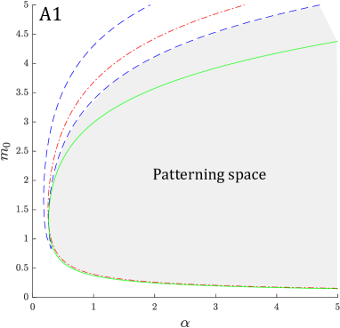
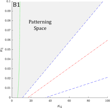
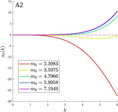
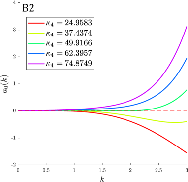
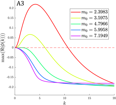
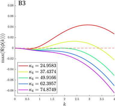
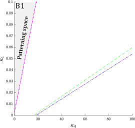
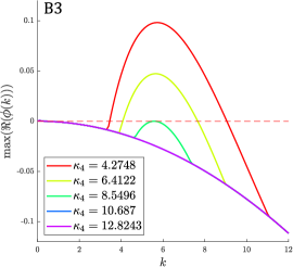
Figure 3.1: Patterning space, parameter condition and dispersion relations for the uncoupled poro-mechano-chemical model. (A1) Predicted pattering space for a selected interval in (m0,α)subscript𝑚0𝛼(m_{0},\alpha) parameter space: (green plain) boundary constructed from (3.7a); (red-dashed) boundary coming from (3.7b); (blue-dot-dashed) boundary built from (3.7c). (A2) Parameter coefficient condition a0subscript𝑎0a_{0}. Curves are drawn from the critical value m0csuperscriptsubscript𝑚0𝑐m_{0}^{c} (green) and for 25% and 50% increase/decrease parameter values. (A3) Associated dispersion relations. Colour code is kept identical with (A2). (B1-B3) Similar analysis for the (κ1,κ4)subscript𝜅1subscript𝜅4(\kappa_{1},\kappa_{4}) parameter space.

Either (3.7a) or (3.7b) enforces that k2superscript𝑘2k^{2} has a real positive part, while (3.7c) is necessary to have a real wave number. These conditions are similar to the ones stated in [36]. The inequality (3.7b) emphasises how the positive feedback mechanism of the accumulation of mesenchymal cells through chemotaxis leads to stimulate further FGF secretion, based on the activation of the epithelium. When the condition is satisfied, patterning is achieved.

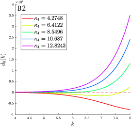
Condition (3.7a) indicates that the steady state is destabilised when Am>0subscript𝐴𝑚0A_{m}>0, occurring when the clustering-mediated activation is sufficiently strong. Figure 3.1 (panels (A1)-(B1)) present the patterning space based on the implicit functions defined in (3.7a)-(3.7c) for the (m0,α)subscript𝑚0𝛼(m_{0},\alpha) and (κ1,κ4)subscript𝜅1subscript𝜅4(\kappa_{1},\kappa_{4}) space. The conditions are represented in both Figures by a plain-green curve (3.7a), a red-dot-dashed curve (3.7b), and a blue-dashed curve (3.7c). The boundaries present very similar results to the linear analysis from [36]. Here, we accentuate the region by filling with light grey. Panels (A2)-(A3) and (B2)-(B3) in Figure 3.1 portray the functions a0(k2)subscript𝑎0superscript𝑘2a_{0}(k^{2}) (parameter condition) and λ(k2)𝜆superscript𝑘2\lambda(k^{2}) (dispersion relation) for the studied parameters m0subscript𝑚0m_{0} and κ4subscript𝜅4\kappa_{4}. We present in different colours the behaviour of the system for the critical parameter value (green curve), as well as parameter values obtained by increasing and decreasing by 25% and 50% the critical value, where we recall that fixed parameters are taken from Table 1. We see that moving above or below the critical value results in a finite interval of wave numbers for which the complex eigenvalue presented positive real component and thus leading to instability (patterning). As illustrated also in [36], for a specific parameter set, panels (A1)-(A3) from Figure 3.1 show that a sufficiently dense dermis cells concentration is necessary to produce instability. While increasing the chemotaxis sensibility of the system we spread the range of possible mesenchymal cells density, by the u-shape form of the boundary, a too-high density cell can lead to prevention of pattern formation (see Figure 3.1 (A1)). The capacity of BMP to deactivate the epithelium by increasing κ4subscript𝜅4\kappa_{4}, drops rapidly the patterning ability of the system.

3.5 Zero activation/inactivation of epithelium.

Different scenarios are possible in such case: only zero activation (κ1=κ2=0subscript𝜅1subscript𝜅20\kappa_{1}=\kappa_{2}=0, e0=0subscript𝑒00e_{0}=0), only zero inactivation (κ3=κ4=0subscript𝜅3subscript𝜅40\kappa_{3}=\kappa_{4}=0, e0=1subscript𝑒01e_{0}=1) or both zero activation and inactivation of the epithelium. Contrary to [36], the coupling to poroelastic structure leads to a more involved analysis of the system and in particular, it does not guarantee that patterning is not predicted. In any case, the coefficients Amsubscript𝐴𝑚A_{m} and Absubscript𝐴𝑏A_{b} will be zero and bring the coefficients of P2subscript𝑃2P_{2} to be strictly positive. As the coefficients of P3subscript𝑃3P_{3} are also non-negative, P(ϕ;k2)𝑃italic-ϕsuperscript𝑘2P(\phi;k^{2}) can only lead to negative eigenvalues if the coefficients of P1subscript𝑃1P_{1} are negative. By Definition 3.2, we know that the bisubscript𝑏𝑖b_{i}’s are negative only if the coupled-dependent constant is itself negative. This occurs when the following conditions are satisfied

(λ+2μ3)τ1ζm02(1+ζm02)2>0{τ>0 and m0<1ζτ<0 and m0>1ζ.-\left(\lambda+\frac{2\mu}{3}\right)\tau\frac{1-\zeta m_{0}^{2}}{\left(1+\zeta m_{0}^{2}\right)^{2}}>0\Leftrightarrow\Bigg{\{}\begin{matrix}\tau>0&\text{ and }&m_{0}<\sqrt{\frac{1}{\zeta}}\\ \tau<0&\text{ and }&m_{0}>\sqrt{\frac{1}{\zeta}}\end{matrix}.

If one of the condition is satisfied, the formation of patterns is expected. This is an opposite conclusion as that drawn in the case of chemotaxis only [36].
Refer to caption
Refer to caption
Refer to caption
Refer to caption
Refer to caption
Refer to caption
Refer to caption
Refer to caption
Refer to caption
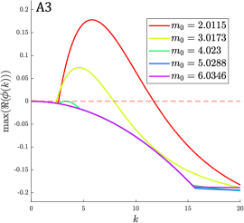
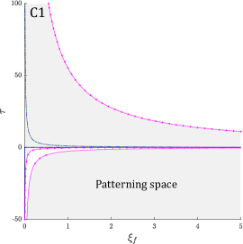
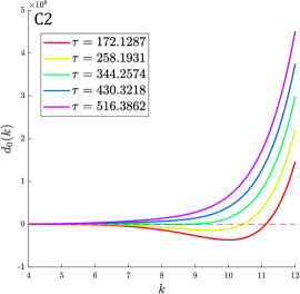
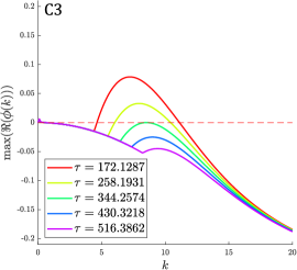
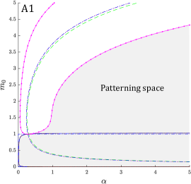
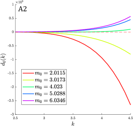
Figure 3.2: Patterning space, parameter condition and dispersion relations for the coupled poro-mechano-chemical model. (A1): predicted pattering space for a selected interval in (m0,α)subscript𝑚0𝛼(m_{0},\alpha). Parameter space: (black plain) boundary built from (3.8a) for θ1subscript𝜃1\theta_{1}; (green-dashed) boundary built from (3.8a) for θ2subscript𝜃2\theta_{2}; (red-dot-dot) boundary built from (3.8b); (blue-dot-dashed) boundary from (3.8c); (magenta-dot-plain) boundary built from (3.9). (A2): Coefficient condition on d0subscript𝑑0d_{0}. Curves are drawn from the critical value m0csuperscriptsubscript𝑚0𝑐m_{0}^{c} (green) and for the 25% and 50% increase/decrease parameter value. (A3): associated dispersion relations. Colour code is kept identical with (A2). (B1-B4): similar analysis for the (κ1,κ4)subscript𝜅1subscript𝜅4(\kappa_{1},\kappa_{4}) parameter space. (C1-C3): similar analysis for the (τ,ξf)𝜏subscript𝜉𝑓(\tau,\xi_{f}) parameter space.

3.6 General case.

The thorough analysis of the coupled system involves a seventh-order polynomial. Analytical Routh–Hurwitz conditions in this case are hardly accessible and the crossed effects due to multiple parameters and conditions will inevitably make difficult the interpretation of the system behaviour. We can however restrict then the analysis to ϕ0superscriptitalic-ϕ0\phi^{0}, with coefficients d0=a0c0+b0subscript𝑑0subscript𝑎0subscript𝑐0subscript𝑏0d_{0}=a_{0}c_{0}+b_{0}, where a0subscript𝑎0a_{0}, b0subscript𝑏0b_{0}, c0subscript𝑐0c_{0} are as in Definition 3.2. After some algebraic manipulations, we derive d0subscript𝑑0d_{0} with respect to k2superscript𝑘2k^{2} and obtain

d0(k2)=θ4k8+θ3k6+θ2k4+θ1k2,superscriptsubscript𝑑0superscript𝑘2subscript𝜃4superscript𝑘8subscript𝜃3superscript𝑘6subscript𝜃2superscript𝑘4subscript𝜃1superscript𝑘2d_{0}^{\prime}(k^{2})=\theta_{4}k^{8}+\theta_{3}k^{6}+\theta_{2}k^{4}+\theta_{1}k^{2},

where

θ1subscript𝜃1\displaystyle\theta_{1} =2ξf(λ+2μ3)τ1ζm02(1+ζm02)2αm0em0(kon+koff),absent2subscript𝜉𝑓𝜆2𝜇3𝜏1𝜁superscriptsubscript𝑚02superscript1𝜁superscriptsubscript𝑚022𝛼subscript𝑚0superscriptesubscript𝑚0subscript𝑘onsubscript𝑘off\displaystyle=-2\xi_{f}\left(\lambda+\frac{2\mu}{3}\right)\tau\frac{1-\zeta m_{0}^{2}}{\left(1+\zeta m_{0}^{2}\right)^{2}}\alpha m_{0}\mathrm{e}^{-m_{0}}(k_{\text{on}}+k_{\text{off}}),
θ2subscript𝜃2\displaystyle\theta_{2} =3[(2μ+λ)(DmδB(kon+koff)+αm0em0H3Abαm0em0Am)\displaystyle=3\Bigg{[}(2\mu+\lambda)\Big{(}D_{m}\delta_{B}(k_{\text{on}}+k_{\text{off}})+\alpha m_{0}\mathrm{e}^{-m_{0}}H_{3}A_{b}-\alpha m_{0}\mathrm{e}^{-m_{0}}A_{m}\Big{)}
ξf(λ+2μ3)τ1ζm02(1+ζm02)2αm0em0(kon+koff)],\displaystyle\qquad-\xi_{f}\left(\lambda+\frac{2\mu}{3}\right)\tau\frac{1-\zeta m_{0}^{2}}{\left(1+\zeta m_{0}^{2}\right)^{2}}\alpha m_{0}\mathrm{e}^{-m_{0}}(k_{\text{on}}+k_{\text{off}})\Bigg{]},
θ3subscript𝜃3\displaystyle\theta_{3} =4(2μ+λ)((DmδB+DmDf)(kon+koff)αm0em0Am),absent42𝜇𝜆subscript𝐷𝑚subscript𝛿𝐵subscript𝐷𝑚subscript𝐷𝑓subscript𝑘onsubscript𝑘off𝛼subscript𝑚0superscriptesubscript𝑚0subscript𝐴𝑚\displaystyle=4(2\mu+\lambda)\left((D_{m}\delta_{B}+D_{m}D_{f})(k_{\text{on}}+k_{\text{off}})-\alpha m_{0}\mathrm{e}^{-m_{0}}A_{m}\right),
θ4subscript𝜃4\displaystyle\theta_{4} =5DmDf(2μ+λ)(kon+koff).absent5subscript𝐷𝑚subscript𝐷𝑓2𝜇𝜆subscript𝑘onsubscript𝑘off\displaystyle=5D_{m}D_{f}(2\mu+\lambda)(k_{\text{on}}+k_{\text{off}}).
Refer to caption
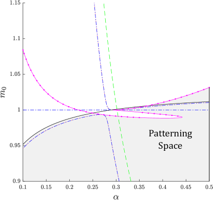
Figure 3.3: Patterning space for the coupled poro-mechano-chemical model. Selected interval in the (m0,α)subscript𝑚0𝛼(m_{0},\alpha) parameter space. (black plain) boundary built from (3.8a) for θ1subscript𝜃1\theta_{1}; (green-dashed) boundary from (3.8a) for θ2subscript𝜃2\theta_{2}; (red-dot-dot) boundary from (3.8b); (blue-dot-dashed) boundary from (3.8c); (magenta-dot-plain) boundary built from (3.9).

In contrast with the uncoupled case studied above, here kc2superscriptsubscript𝑘𝑐2k_{c}^{2} is found by solving a quartic polynomial (employing the intrinsic MATLAB function roots, after constructing the associated vector of polynomial coefficients). In addition, one needs to satisfy some additional conditions leading to d0<0subscript𝑑00d_{0}<0 for any positive k2superscript𝑘2k^{2}. More specifically, the constrains consist on at least one of the Routh–Hurwitz conditions [40], stated as

θ1>0,θ2>0,θ3formulae-sequencesubscript𝜃10subscript𝜃20subscript𝜃3\displaystyle\theta_{1}>0,\qquad\theta_{2}>0,\qquad\theta_{3} >0,absent0\displaystyle>0, (3.8a)
θ2θ3θ1θ4subscript𝜃2subscript𝜃3subscript𝜃1subscript𝜃4\displaystyle\theta_{2}\theta_{3}-\theta_{1}\theta_{4} >0,absent0\displaystyle>0, (3.8b)
θ1θ2θ3θ12θ4subscript𝜃1subscript𝜃2subscript𝜃3superscriptsubscript𝜃12subscript𝜃4\displaystyle\theta_{1}\theta_{2}\theta_{3}-\theta_{1}^{2}\theta_{4} >0,absent0\displaystyle>0, (3.8c)

or the discriminant

27θ42θ14+18θ4θ3θ2θ134θ4θ23θ134θ33θ13+θ32θ22θ12>0.27superscriptsubscript𝜃42superscriptsubscript𝜃1418subscript𝜃4subscript𝜃3subscript𝜃2superscriptsubscript𝜃134subscript𝜃4superscriptsubscript𝜃23superscriptsubscript𝜃134superscriptsubscript𝜃33superscriptsubscript𝜃13superscriptsubscript𝜃32superscriptsubscript𝜃22superscriptsubscript𝜃120-27\theta_{4}^{2}\theta_{1}^{4}+18\theta_{4}\theta_{3}\theta_{2}\theta_{1}^{3}-4\theta_{4}\theta_{2}^{3}\theta_{1}^{3}-4\theta_{3}^{3}\theta_{1}^{3}+\theta_{3}^{2}\theta_{2}^{2}\theta_{1}^{2}>0. (3.9)

Condition (3.8b) highlights the effect of poromechanics towards the instability of the system, in comparison against the uncoupled cased. Increasing the influence of the mesenchymal cells through τ𝜏\tau, or the influence of mechanics on f𝑓f through ξfsubscript𝜉𝑓\xi_{f}, can relax the requirement that the feedback-positive loop from (3.7b) should be sufficiently strong to create instability. As mentioned in the activation/inactivation of epithelium scenario, this will depend mostly on the sign of the active stress component of the coefficient, and thus on the sign of τ𝜏\tau and the value of m0subscript𝑚0m_{0}, see Figure 3.2(C1). The dispersion relation for the (m0,α)subscript𝑚0𝛼(m_{0},\alpha)- and (κ1,κ2)subscript𝜅1subscript𝜅2(\kappa_{1},\kappa_{2})– parameter spaces illustrates how, for the same fixed set of parameters from Table 1, the poromechanical coupling leads to a decrease of the critical parameter value (Figures 3.2(A3) and (B3)). Unfortunately, the ease to push the system to instability is counter-balanced by a more restrictive space of parameters values where patterns can be formed (more precisely, compared to Figures 3.1(A1),(B1) and 3.2 (A1),(B1),(C1)). This can increase the difficulty in tuning parameters to produce specific patterns. Indeed, zooming into the parameters-pair (m0,α)subscript𝑚0𝛼(m_{0},\alpha) on the region where the boundary conditions cross (see Figure 3.3), exposes how easily the patterns can disappear after a relatively small variation in parameter values.

4 Extension to finite-strain poroelasticity and growth

We briefly recall some kinematic considerations, needed in order to incorporate growth effects. Thorough reviews of mechanical models for growth of soft living tissues can be found in [22, 25]. Let us denote by 𝐗𝐗\mathbf{X} the position of a material point in the reference (or initial) configuration (region Ω0subscriptΩ0\Omega_{0} with boundary Ω0=Γ0Σ0subscriptΩ0subscriptΓ0subscriptΣ0\partial\Omega_{0}=\Gamma_{0}\cup\Sigma_{0} and outward pointing unit normal 𝐍0subscript𝐍0\mathbf{N}_{0}) and let 𝒙=𝝋(𝐗)𝒙𝝋𝐗\boldsymbol{x}=\boldsymbol{\varphi}(\mathbf{X}) denote its position at time t𝑡t in the current configuration of the domain, ΩΩ\Omega, determined by the deformation mapping 𝝋(,t):Ω0Ω:𝝋𝑡subscriptΩ0Ω\boldsymbol{\varphi}(\cdot,t):\Omega_{0}\to\Omega. We adopt the notation 𝐃𝐢𝐯,Div𝐃𝐢𝐯Div\mathop{\mathbf{Div}}\nolimits,\mathop{\mathrm{Div}}\nolimits for the divergence of tensor and vector fields, and 𝐆𝐫𝐚𝐝,Grad𝐆𝐫𝐚𝐝Grad\mathop{\mathbf{Grad}}\nolimits,\mathop{\mathrm{Grad}}\nolimits for the gradients of vector and scalar fields, respectively; all with respect to the material coordinates. The geometric deformation tensor is 𝐅=𝐆𝐫𝐚𝐝𝝋=𝐈+𝐆𝐫𝐚𝐝𝒖𝐅𝐆𝐫𝐚𝐝𝝋𝐈𝐆𝐫𝐚𝐝𝒖\mathbf{F}=\mathop{\mathbf{Grad}}\nolimits\boldsymbol{\varphi}=\mathbf{I}+\mathop{\mathbf{Grad}}\nolimits\boldsymbol{u} (where the gradient of the deformation map and of the displacement field is taken with respect to the reference coordinates) and its Jacobian is J=det𝐅>0𝐽𝐅0J=\det\mathbf{F}>0. The velocity in Lagrangian coordinates is denoted as 𝒗=𝒖˙𝒗˙𝒖\boldsymbol{v}=\dot{\boldsymbol{u}}, and 𝐂=𝐅𝐅𝐂superscript𝐅𝐅\mathbf{C}=\mathbf{F}^{\intercal}\mathbf{F} is the right Cauchy–Green strain tensor.

As in the linearised regime, we assume that the region occupied by the tissue is fully saturated, and consisting of a fluid and of a solid phase:

ϕf+ϕs=1,subscriptitalic-ϕ𝑓subscriptitalic-ϕ𝑠1\phi_{f}+\phi_{s}=1, (4.1)

where the ϕjsubscriptitalic-ϕ𝑗\phi_{j}’s denote the volume fraction of each phase. The phase s𝑠s is assumed a neo–Hookean solid whereas the liquid phase is considered as an ideal fluid. Both phases are assumed intrinsically incompressible. The expected growth is due to proliferation of cells, and implying a mass exchange between the phases. The mass balances in the Eulerian framework assume the form

ϕst+div(ϕs𝒗s)subscriptitalic-ϕ𝑠𝑡divsubscriptitalic-ϕ𝑠subscript𝒗𝑠\displaystyle\frac{\partial\phi_{s}}{\partial t}+\mathop{\mathrm{div}}\nolimits(\phi_{s}\boldsymbol{v}_{s}) =rs,absentsubscript𝑟𝑠\displaystyle=r_{s}, (4.2a)
ϕft+div(ϕf𝒗f)subscriptitalic-ϕ𝑓𝑡divsubscriptitalic-ϕ𝑓subscript𝒗𝑓\displaystyle\frac{\partial\phi_{f}}{\partial t}+\mathop{\mathrm{div}}\nolimits(\phi_{f}\boldsymbol{v}_{f}) =rs,absentsubscript𝑟𝑠\displaystyle=-r_{s}, (4.2b)

with 𝒗s,𝒗fsubscript𝒗𝑠subscript𝒗𝑓\boldsymbol{v}_{s},\boldsymbol{v}_{f} the Eulerian velocities in each phase, and rs=α0ϕs(1ϕs)(mm0)subscript𝑟𝑠subscript𝛼0subscriptitalic-ϕ𝑠1subscriptitalic-ϕ𝑠𝑚subscript𝑚0r_{s}=\alpha_{0}\phi_{s}(1-\phi_{s})(m-m_{0}) being the mass growth rate (net proliferation rate of cells in the solid phase), here assumed linearly dependent on the concentration of mesynchemal cells and decreasing as the available space decreases. In turn, the general form of the momentum balances is

𝐝𝐢𝐯(ϕs𝝈eff,s)ϕsp+𝒇sf𝐝𝐢𝐯subscriptitalic-ϕ𝑠subscript𝝈eff𝑠subscriptitalic-ϕ𝑠𝑝subscript𝒇𝑠𝑓\displaystyle\mathop{\mathbf{div}}\nolimits(\phi_{s}\boldsymbol{\sigma}_{\mathrm{eff},s})-\phi_{s}\nabla p+\boldsymbol{f}_{sf} =𝟎,absent0\displaystyle=\boldsymbol{0},
𝐝𝐢𝐯(ϕf𝝈eff,f)ϕfp+𝒇fs𝐝𝐢𝐯subscriptitalic-ϕ𝑓subscript𝝈eff𝑓subscriptitalic-ϕ𝑓𝑝subscript𝒇𝑓𝑠\displaystyle\mathop{\mathbf{div}}\nolimits(\phi_{f}\boldsymbol{\sigma}_{\mathrm{eff},f})-\phi_{f}\nabla p+\boldsymbol{f}_{fs} =𝟎,absent0\displaystyle=\boldsymbol{0},

where the 𝝈eff,jsubscript𝝈eff𝑗\boldsymbol{\sigma}_{\mathrm{eff},j}’s are the respective effective Cauchy stresses, p𝑝p is the average pressure of the liquid phase, and

𝒇sf=pϕs+η/κϕsϕf(𝒗f𝒗s),𝒇fs=pϕfη/κϕfϕs(𝒗f𝒗s),formulae-sequencesubscript𝒇𝑠𝑓𝑝subscriptitalic-ϕ𝑠𝜂𝜅subscriptitalic-ϕ𝑠subscriptitalic-ϕ𝑓subscript𝒗𝑓subscript𝒗𝑠subscript𝒇𝑓𝑠𝑝subscriptitalic-ϕ𝑓𝜂𝜅subscriptitalic-ϕ𝑓subscriptitalic-ϕ𝑠subscript𝒗𝑓subscript𝒗𝑠\boldsymbol{f}_{sf}=p\nabla\phi_{s}+\eta/\kappa\phi_{s}\phi_{f}(\boldsymbol{v}_{f}-\boldsymbol{v}_{s}),\quad\boldsymbol{f}_{fs}=p\nabla\phi_{f}-\eta/\kappa\phi_{f}\phi_{s}(\boldsymbol{v}_{f}-\boldsymbol{v}_{s}),

are the respective drag terms and net sources of momentum, where κ,η𝜅𝜂\kappa,\eta are the permeability and dynamic viscosity, respectively. The effective stress of the liquid phase 𝝈eff,fsubscript𝝈eff𝑓\boldsymbol{\sigma}_{\mathrm{eff},f} is assumed negligible with respect to the interstitial pressure gradient and therefore the mixture stress is 𝝈eff=𝝈eff,ssubscript𝝈effsubscript𝝈eff𝑠\boldsymbol{\sigma}_{\mathrm{eff}}=\boldsymbol{\sigma}_{\mathrm{eff},s}. In addition, Darcy’s law gives

𝒗f𝒗s=κηϕfp,subscript𝒗𝑓subscript𝒗𝑠𝜅𝜂subscriptitalic-ϕ𝑓𝑝\boldsymbol{v}_{f}-\boldsymbol{v}_{s}=-\frac{\kappa}{\eta\phi_{f}}\nabla p, (4.3)

and then the mixture momentum balance is written as

𝐝𝐢𝐯(𝝈eff)+p=𝟎in Ω×(0,tfinal].𝐝𝐢𝐯subscript𝝈eff𝑝0in Ω0subscript𝑡final-\mathop{\mathbf{div}}\nolimits(\boldsymbol{\sigma}_{\mathrm{eff}})+\nabla p=\boldsymbol{0}\qquad\text{in }\Omega\times(0,t_{\mathrm{final}}]. (4.4)

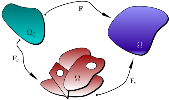
The deformation mapping can be decomposed into a purely growth part and the remainder, elastic, deformation. Such splitting implies that there exists an intermediate configuration Ω~~Ω\widetilde{\Omega} between Ω0subscriptΩ0\Omega_{0} and ΩΩ\Omega which is not necessarily compatible (and which we assume is completely stress free, see sketch in Figure 4.1), and consequently a multiplicative decomposition of the deformation gradient into a growth deformation gradient (describing local generation or removal of material points) and an elastic deformation gradient tensor is admitted (see, for instance, [26, 39, 23])

𝐅=𝐅e𝐅g,𝐅subscript𝐅𝑒subscript𝐅𝑔\mathbf{F}=\mathbf{F}_{e}\mathbf{F}_{g}, (4.5)

and therefore J=JeJg𝐽subscript𝐽𝑒subscript𝐽𝑔J=J_{e}J_{g} with Je:=det𝐅eassignsubscript𝐽𝑒subscript𝐅𝑒J_{e}:=\det\mathbf{F}_{e}, Jg:=det𝐅gassignsubscript𝐽𝑔subscript𝐅𝑔J_{g}:=\det\mathbf{F}_{g}. Note also that since 𝐅𝐅\mathbf{F} is assumed nonsingular, so are the tensors 𝐅e,𝐅gsubscript𝐅𝑒subscript𝐅𝑔\mathbf{F}_{e},\mathbf{F}_{g}.

Refer to caption
Figure 4.1: Decomposition of the tensor gradient of deformation 𝐅𝐅\mathbf{F} into pure growth 𝐅gsubscript𝐅𝑔\mathbf{F}_{g} and an elastic deformation tensor 𝐅esubscript𝐅𝑒\mathbf{F}_{e}. The intermediate configuration Ω~~Ω\widetilde{\Omega}, between the undeformed reference state Ω0subscriptΩ0\Omega_{0} and the current/final configuration ΩΩ\Omega including growth and elastic response with stress, is an incompatible and stress-free growth state.

Since the intermediate configuration is considered stress-free, stresses are exerted only by the elastic deformation, and the constitutive relations between a given strain energy function ΨΨ\Psi (that characterises the material response of the solid for hyperelastic materials) and the measures of stress can be stated with respect to the intermediate configuration Ω~~Ω\widetilde{\Omega}. For the Cauchy stress this gives

𝝈eff=2Je1𝐅eΨ𝐂e𝐅e,subscript𝝈eff2superscriptsubscript𝐽𝑒1subscript𝐅𝑒Ψsubscript𝐂𝑒superscriptsubscript𝐅𝑒absent\boldsymbol{\sigma}_{\mathrm{eff}}=2J_{e}^{-1}\mathbf{F}_{e}\frac{\partial\Psi}{\partial\mathbf{C}_{e}}\mathbf{F}_{e}^{-\intercal}, (4.6)

where 𝐂e=𝐅e𝐅esubscript𝐂𝑒superscriptsubscript𝐅𝑒subscript𝐅𝑒\mathbf{C}_{e}=\mathbf{F}_{e}^{\intercal}\mathbf{F}_{e} and Je=det(𝐅𝐅g1)subscript𝐽𝑒superscriptsubscript𝐅𝐅𝑔1J_{e}=\det(\mathbf{F}\mathbf{F}_{g}^{-1}) is the reversible part of the Jacobian. This constitutive equation requires to describe also 𝐅𝐅\mathbf{F} and 𝐅gsubscript𝐅𝑔\mathbf{F}_{g}, but from the relation 𝐅˙𝐅1=𝒗s˙𝐅superscript𝐅1bold-∇subscript𝒗𝑠\dot{\mathbf{F}}{\mathbf{F}^{-1}}=\boldsymbol{\nabla}\boldsymbol{v}_{s}, we realise that only 𝐅gsubscript𝐅𝑔\mathbf{F}_{g} needs to be specified.

In order to translate equations (4.2a)-(4.6) into Lagrangian form, we recall the change in volume and area relations dV=JdV0d𝑉𝐽dsubscript𝑉0\mathrm{d}V=J\mathrm{d}V_{0} and dS=J𝐅dS0d𝑆𝐽superscript𝐅absentdsubscript𝑆0\mathrm{d}S=J\mathbf{F}^{-\intercal}\mathrm{d}S_{0} together with the transformation of unit outward normal vectors 𝒏=𝐅𝐍0𝒏superscript𝐅absentsubscript𝐍0\boldsymbol{n}=\mathbf{F}^{-\intercal}\mathbf{N}_{0}. For the solid mass balance (4.2a) it suffices to apply Reynolds transport theorem, the change of coordinates, and Maxwell’s localisation to obtain

Jϕs¯˙=Jrs.˙¯𝐽subscriptitalic-ϕ𝑠𝐽subscript𝑟𝑠\dot{\overline{J\phi_{s}}}=Jr_{s}. (4.7)

The Lagrangian form of Darcy’s law

𝒗f𝒗s=𝐅κηϕf𝐂1Gradp,subscript𝒗𝑓subscript𝒗𝑠𝐅𝜅𝜂subscriptitalic-ϕ𝑓superscript𝐂1Grad𝑝\boldsymbol{v}_{f}-\boldsymbol{v}_{s}=-\mathbf{F}\frac{\kappa}{\eta\phi_{f}}\mathbf{C}^{-1}\mathop{\mathrm{Grad}}\nolimits p, (4.8)

results from (4.3) in combination with transport, localisation, as well as pull-back operations. For the liquid mass balance (4.2b), one can apply the generalised Reynolds transport theorem, (4.8), divergence’s theorem, and localisation, to arrive at

Jϕf¯˙+Div(Jκη𝐂1Gradp)=Jrs.˙¯𝐽subscriptitalic-ϕ𝑓Div𝐽𝜅𝜂superscript𝐂1Grad𝑝𝐽subscript𝑟𝑠\dot{\overline{J\phi_{f}}}+\mathop{\mathrm{Div}}\nolimits(J\frac{\kappa}{\eta}\mathbf{C}^{-1}\mathop{\mathrm{Grad}}\nolimits p)=-Jr_{s}. (4.9)

Summing up (4.7) and (4.9) and taking an approximation of the fluid volume fraction in terms of fluid pressure and volume change we obtain (4.12b), below.

For transforming the momentum balance (4.4) we use the divergence theorem, the change of coordinates, we recall the relation between Cauchy and first Piola–Kirchhoff stress 𝐏=J𝝈𝐅𝐏𝐽𝝈superscript𝐅\mathbf{P}=J\boldsymbol{\sigma}\mathbf{F}^{\intercal}, and use again the divergence theorem to get (4.12a), below. The hyperelastic component to the stress is

𝐏e=Ψ𝐅|Ω~,subscript𝐏𝑒evaluated-atΨ𝐅~Ω\mathbf{P}_{e}=\frac{\partial\Psi}{\partial\mathbf{F}}|_{\widetilde{\Omega}}, (4.10)

and for a neo–Hookean material, equations (4.5)-(4.10) imply that the effective stress tensor is

𝐏e=J(μ𝐁eψ𝐈)𝐅,subscript𝐏𝑒𝐽𝜇subscript𝐁𝑒𝜓𝐈superscript𝐅absent\mathbf{P}_{e}=J(\mu\mathbf{B}_{e}-\psi\mathbf{I})\mathbf{F}^{-\intercal}, (4.11)

where μ𝜇\mu is the shear modulus, ψ𝜓\psi denotes a Lagrange multiplier, and 𝐁e=𝐅e𝐅esubscript𝐁𝑒subscript𝐅𝑒superscriptsubscript𝐅𝑒\mathbf{B}_{e}=\mathbf{F}_{e}\mathbf{F}_{e}^{\intercal} is the right Cauchy–Green deformation tensor associated with the intermediate configuration Ω~~Ω\widetilde{\Omega}. Note that in this context, rather than material incompressibility of the mixture, the Lagrange multiplier ψ𝜓\psi enforces a mass conservation kinematic constraint of the form Je=1subscript𝐽𝑒1J_{e}=1, confirming that for a hyperelastically incompressible material all volume changes are solely due to growth factors (Jg=det𝐅gsubscript𝐽𝑔subscript𝐅𝑔J_{g}=\det\mathbf{F}_{g} is in turn irreversible) [6]. If Jg>1subscript𝐽𝑔1J_{g}>1 the body undergoes growth.

In summary, the equations of nonlinear poroelasticity with growth (including momentum conservation of the solid-fluid mixture, fluid mass balance, and incompressibility of elastic deformations) read as follows

ρ𝒖¨𝐃𝐢𝐯(𝐏e+𝐏f)𝜌¨𝒖𝐃𝐢𝐯subscript𝐏𝑒subscript𝐏𝑓\displaystyle\rho\ddot{\boldsymbol{u}}-\mathop{\mathbf{Div}}\nolimits(\mathbf{P}_{e}+\mathbf{P}_{f}) =𝟎absent0\displaystyle=\boldsymbol{0} in Ω0×(0,tfinal],in subscriptΩ00subscript𝑡final\displaystyle\text{in }\Omega_{0}\times(0,t_{\mathrm{final}}], (4.12a)
(C0p+αBW[tr𝐂d])¯˙1JDiv(κηJ𝐂1Gradp)˙¯subscript𝐶0𝑝subscript𝛼𝐵𝑊delimited-[]tr𝐂𝑑1𝐽Div𝜅𝜂𝐽superscript𝐂1Grad𝑝\displaystyle\dot{\overline{\bigl{(}C_{0}p+\alpha_{BW}[\mathop{\mathrm{tr}}\nolimits\mathbf{C}-d]\bigr{)}}}-\frac{1}{J}\mathop{\mathrm{Div}}\nolimits\biggl{(}\frac{\kappa}{\eta}J\mathbf{C}^{-1}\mathop{\mathrm{Grad}}\nolimits p\biggr{)} =absent\displaystyle=\ell in Ω0×(0,tfinal],in subscriptΩ00subscript𝑡final\displaystyle\text{in }\Omega_{0}\times(0,t_{\mathrm{final}}], (4.12b)
Jesubscript𝐽𝑒\displaystyle J_{e} =1absent1\displaystyle=1 in Ω0×(0,tfinal],in subscriptΩ00subscript𝑡final\displaystyle\text{in }\Omega_{0}\times(0,t_{\mathrm{final}}], (4.12c)

where the stress exerted by the fluid (when pulled back to the reference configuration) is simply 𝐏f=αBWJp𝐅subscript𝐏𝑓subscript𝛼𝐵𝑊𝐽𝑝superscript𝐅absent\mathbf{P}_{f}=-\alpha_{BW}Jp\mathbf{F}^{-\intercal}, and the divergence and gradient operators are now understood with respect to the undeformed coordinates. In contrast with the model from Section 2, now the fluid has a source that we relate to the growth process and make it precise below. The divergence of displacement accompanying the Biot–Willis constant has now been replaced by tr𝐂dtr𝐂𝑑\mathop{\mathrm{tr}}\nolimits\mathbf{C}-d, where d𝑑d is the spatial dimension.

It remains to characterise the growth deformation gradient. We suppose that growth occurs due to a set of internal variables γ1,γ2,γ3subscript𝛾1subscript𝛾2subscript𝛾3\gamma_{1},\gamma_{2},\gamma_{3} acting on local orthonormal directions 𝒌1subscript𝒌1\boldsymbol{k}_{1}, 𝒌2subscript𝒌2\boldsymbol{k}_{2}, 𝒌3subscript𝒌3\boldsymbol{k}_{3} in the undeformed configuration (and in 2D we consider only γ1,γ2subscript𝛾1subscript𝛾2\gamma_{1},\gamma_{2} acting on 𝒌1subscript𝒌1\boldsymbol{k}_{1}, 𝒌2subscript𝒌2\boldsymbol{k}_{2}, respectively), and a general form for the growth deformation tensor is simply

𝐅g=𝐈+γ1𝒌1𝒌1+γ2𝒌2𝒌2+γ3𝒌3𝒌3.subscript𝐅𝑔𝐈tensor-productsubscript𝛾1subscript𝒌1subscript𝒌1tensor-productsubscript𝛾2subscript𝒌2subscript𝒌2tensor-productsubscript𝛾3subscript𝒌3subscript𝒌3\mathbf{F}_{g}=\mathbf{I}+\sqrt{\gamma_{1}}\,\boldsymbol{k}_{1}\otimes\boldsymbol{k}_{1}+\sqrt{\gamma_{2}}\,\boldsymbol{k}_{2}\otimes\boldsymbol{k}_{2}+\gamma_{3}\boldsymbol{k}_{3}\otimes\boldsymbol{k}_{3}.

Assuming that a transversely isotropic growth due to a constant rate occurs on the plane (𝒌1,𝒌2)subscript𝒌1subscript𝒌2(\boldsymbol{k}_{1},\boldsymbol{k}_{2}) and the growth due to morphogen concentrations acts mainly on the direction 𝒌3subscript𝒌3\boldsymbol{k}_{3}, we employ the following specification for the growth factors γisubscript𝛾𝑖\gamma_{i}:

γ1=δ1t,γ2=δ1t,γ3=δ2t+δ3m1+m2,formulae-sequencesubscript𝛾1subscript𝛿1𝑡formulae-sequencesubscript𝛾2subscript𝛿1𝑡subscript𝛾3subscript𝛿2𝑡subscript𝛿3𝑚1superscript𝑚2\gamma_{1}=\delta_{1}t,\quad\gamma_{2}=\delta_{1}t,\quad\gamma_{3}=\delta_{2}t+\delta_{3}\frac{m}{1+m^{2}}, (4.13)

where δ1,δ2,δ3subscript𝛿1subscript𝛿2subscript𝛿3\delta_{1},\delta_{2},\delta_{3} are positive constants and we recall that m𝑚m is the concentration of mesenchymal cells in the form used in the active stress from (2.5). In the 2D case, (4.13) will be replaced by

γ1=γ2=δ2t+δ3m1+m2.subscript𝛾1subscript𝛾2subscript𝛿2𝑡subscript𝛿3𝑚1superscript𝑚2\gamma_{1}=\gamma_{2}=\delta_{2}t+\delta_{3}\frac{m}{1+m^{2}}. (4.14)

As in [16, 30] a more general description that defines a functional relation between the rates of the growth factors and the exchange of mass implies a dependence on the solid volume fraction

i=1dγi˙γi=rsϕs.superscriptsubscript𝑖1𝑑˙subscript𝛾𝑖subscript𝛾𝑖subscript𝑟𝑠subscriptitalic-ϕ𝑠\sum_{i=1}^{d}\frac{\dot{\gamma_{i}}}{\gamma_{i}}=\frac{r_{s}}{\phi_{s}}.

Following [19], we can write a constitutive equation for the mass source in (4.12b) depending on the constants γisubscript𝛾𝑖\gamma_{i} as follows

=0(2δ1+δ2+δ3m(γ3)tm),subscript02subscript𝛿1subscript𝛿2subscript𝛿3subscript𝑚subscript𝛾3subscript𝑡𝑚\ell=\ell_{0}(2\delta_{1}+\delta_{2}+\delta_{3}\partial_{m}(\gamma_{3})\partial_{t}m), (4.15)

where 0subscript0\ell_{0} is a constant and where we stress that ρ𝜌\rho in this section refers to the density of the solid in the reference configuration.

The set of equations is complemented with suitable boundary and initial conditions, formulated in the reference configuration. In contrast with (2.7b)-(2.7c), here we impose Robin conditions for the poroelasticity on the whole undeformed boundary

(𝐏e+𝐏f)𝐍0+ξRJ𝐅𝒖subscript𝐏𝑒subscript𝐏𝑓subscript𝐍0subscript𝜉𝑅𝐽superscript𝐅absent𝒖\displaystyle(\mathbf{P}_{e}+\mathbf{P}_{f})\mathbf{N}_{0}+\xi_{R}J\mathbf{F}^{-\intercal}\boldsymbol{u} =𝟎on (Γ0Σ0)×(0,tfinal],absent0on subscriptΓ0subscriptΣ00subscript𝑡final\displaystyle=\boldsymbol{0}\quad\hbox{on }\quad(\Gamma_{0}\cup\Sigma_{0})\times(0,t_{\text{final}}], (4.16a)
κηJ𝐂1Gradp𝐍0𝜅𝜂𝐽superscript𝐂1Grad𝑝subscript𝐍0\displaystyle\frac{\kappa}{\eta}J\mathbf{C}^{-1}\mathop{\mathrm{Grad}}\nolimits p\cdot\mathbf{N}_{0} =0on Γ0×(0,tfinal],p=pDon Σ0×(0,tfinal],formulae-sequenceabsent0on subscriptΓ00subscript𝑡final𝑝subscript𝑝𝐷on subscriptΣ00subscript𝑡final\displaystyle=0\quad\hbox{on }\quad\Gamma_{0}\times(0,t_{\text{final}}],\qquad p=p_{D}\quad\hbox{on }\quad\Sigma_{0}\times(0,t_{\text{final}}], (4.16b)

where ξRsubscript𝜉𝑅\xi_{R} is the stiffness of the springs attached to Ω0subscriptΩ0\partial\Omega_{0}.

Also the chemotaxis system is recast in the reference domain. In particular, the advection terms are absorbed by the material derivatives (since we are assuming that all species are transported by the whole mixture and can diffuse in both phases) and the diffusion coefficients are modified by the Piola transformation. As in (4.12b), the divergence of displacement in the sink term from (2.3c) now is replaced by tr𝐂dtr𝐂𝑑\mathop{\mathrm{tr}}\nolimits\mathbf{C}-d. The transformation also involves Reynolds transport theorem, divergence theorem, and localisation. Assuming that Dm,Df,Dbsubscript𝐷𝑚subscript𝐷𝑓subscript𝐷𝑏D_{m},D_{f},D_{b} are isotropic, we have

m˙1JDiv(DmJ𝐂1Gradmαmexp(γm)J𝐂1Gradf)˙𝑚1𝐽Divsubscript𝐷𝑚𝐽superscript𝐂1Grad𝑚𝛼𝑚𝛾𝑚𝐽superscript𝐂1Grad𝑓\displaystyle\dot{m}-\frac{1}{J}\mathop{\mathrm{Div}}\nolimits\bigl{(}D_{m}J\mathbf{C}^{-1}\,\mathop{\mathrm{Grad}}\nolimits m-\alpha m\exp(-\gamma m)J\mathbf{C}^{-1}\mathop{\mathrm{Grad}}\nolimits f\bigr{)} =0absent0\displaystyle=0 in Ω0×(0,tfinal],in subscriptΩ00subscript𝑡final\displaystyle\text{in }\Omega_{0}\times(0,t_{\mathrm{final}}], (4.17a)
e˙[κ1w(𝐗,t)h1(m)+κ2h2(m)](1e)+[1h1(m)](κ3+κ4b)e˙𝑒delimited-[]subscript𝜅1𝑤𝐗𝑡subscript1𝑚subscript𝜅2subscript2𝑚1𝑒delimited-[]1subscript1𝑚subscript𝜅3subscript𝜅4𝑏𝑒\displaystyle\dot{e}-[\kappa_{1}w(\mathbf{X},t)h_{1}(m)+\kappa_{2}h_{2}(m)](1-e)+[1-h_{1}(m)](\kappa_{3}+\kappa_{4}b)e =0absent0\displaystyle=0 in Ω0×(0,tfinal],in subscriptΩ00subscript𝑡final\displaystyle\text{in }\Omega_{0}\times(0,t_{\mathrm{final}}], (4.17b)
f˙1JDiv(DfJ𝐂1Gradf)κFe+δFf+ξf(tr𝐂d)˙𝑓1𝐽Divsubscript𝐷𝑓𝐽superscript𝐂1Grad𝑓subscript𝜅𝐹𝑒subscript𝛿𝐹𝑓subscript𝜉𝑓tr𝐂𝑑\displaystyle\dot{f}-\frac{1}{J}\mathop{\mathrm{Div}}\nolimits\bigl{(}D_{f}J\mathbf{C}^{-1}\,\mathop{\mathrm{Grad}}\nolimits f\bigr{)}-\kappa_{F}e+\delta_{F}f+\xi_{f}(\mathop{\mathrm{tr}}\nolimits\mathbf{C}-d) =0absent0\displaystyle=0 in Ω0×(0,tfinal],in subscriptΩ00subscript𝑡final\displaystyle\text{in }\Omega_{0}\times(0,t_{\mathrm{final}}], (4.17c)
b˙1JDiv(DbJ𝐂1Gradb)κBh3(m)m+δBb˙𝑏1𝐽Divsubscript𝐷𝑏𝐽superscript𝐂1Grad𝑏subscript𝜅𝐵subscript3𝑚𝑚subscript𝛿𝐵𝑏\displaystyle\dot{b}-\frac{1}{J}\mathop{\mathrm{Div}}\nolimits\bigl{(}D_{b}J\mathbf{C}^{-1}\,\mathop{\mathrm{Grad}}\nolimits b\bigr{)}-\kappa_{B}h_{3}(m)m+\delta_{B}b =0absent0\displaystyle=0 in Ω0×(0,tfinal],in subscriptΩ00subscript𝑡final\displaystyle\text{in }\Omega_{0}\times(0,t_{\mathrm{final}}], (4.17d)

where divergence and gradients are taken with respect to the undeformed configuration, and the zero-flux boundary conditions (2.7a) are changed accordingly

(DmJ𝐂1Gradmαmexp(γm)J𝐂1Gradf)𝐍0subscript𝐷𝑚𝐽superscript𝐂1Grad𝑚𝛼𝑚𝛾𝑚𝐽superscript𝐂1Grad𝑓subscript𝐍0\displaystyle\bigl{(}D_{m}J\mathbf{C}^{-1}\mathop{\mathrm{Grad}}\nolimits m-\alpha m\exp(-\gamma m)J\mathbf{C}^{-1}\mathop{\mathrm{Grad}}\nolimits f\bigr{)}\cdot\mathbf{N}_{0} =DfJ𝐂1Gradf𝐍0absentsubscript𝐷𝑓𝐽superscript𝐂1Grad𝑓subscript𝐍0\displaystyle=D_{f}J\mathbf{C}^{-1}\mathop{\mathrm{Grad}}\nolimits f\cdot\mathbf{N}_{0}
=DmJ𝐂1Gradm𝐍0absentsubscript𝐷𝑚𝐽superscript𝐂1Grad𝑚subscript𝐍0\displaystyle=D_{m}J\mathbf{C}^{-1}\mathop{\mathrm{Grad}}\nolimits m\cdot\mathbf{N}_{0}
=0on Ω0×(0,tfinal].absent0on Ω0×(0,tfinal]\displaystyle=0\qquad\text{on $\partial\Omega_{0}\times(0,t_{\text{final}}]$}.

5 Numerical tests

Refer to caption
Refer to caption
Refer to caption
Refer to caption
Refer to caption
Refer to caption
Refer to caption
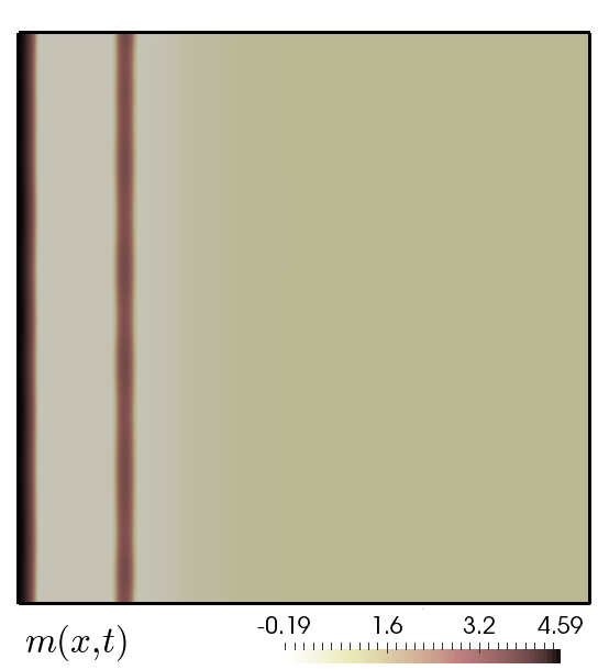
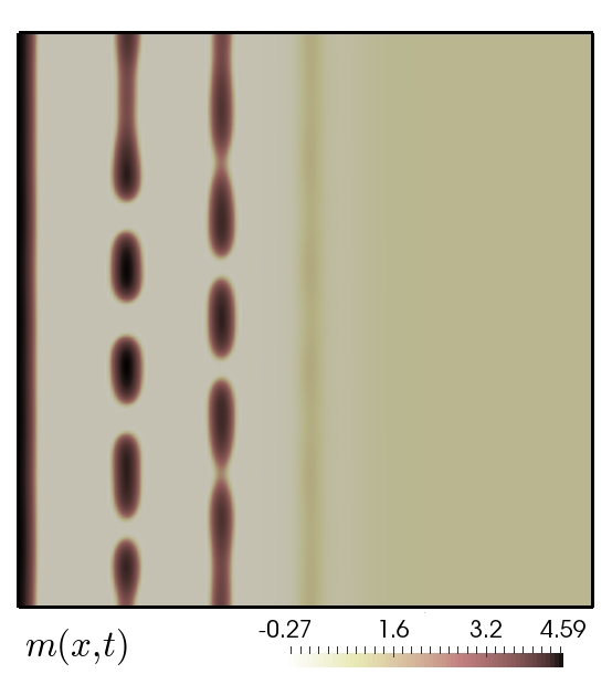
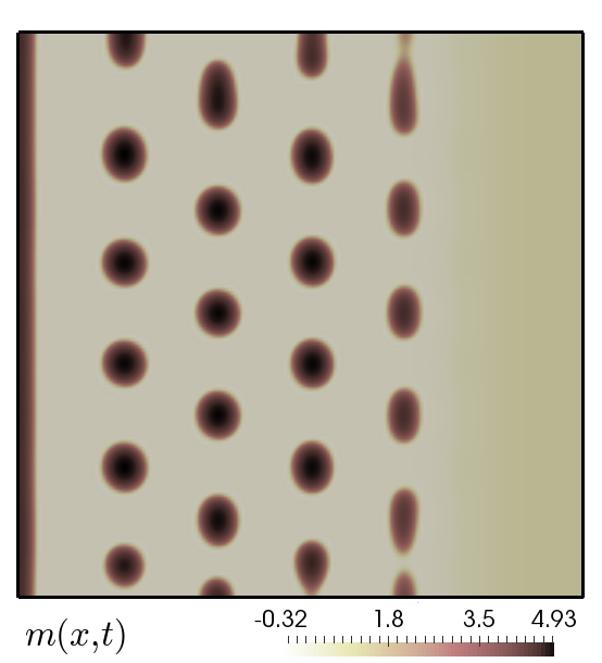
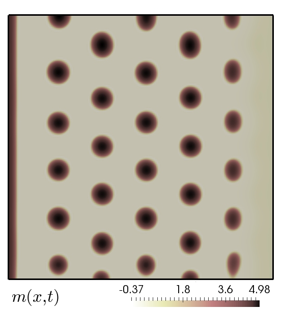
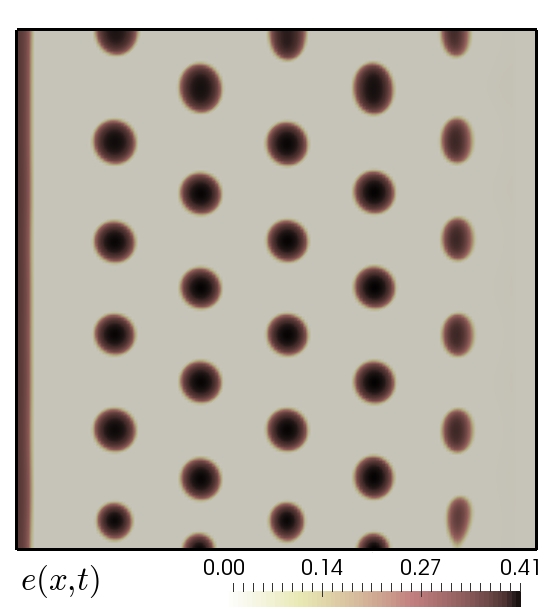
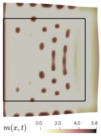
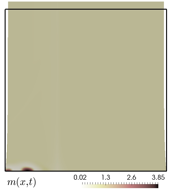
Figure 5.1: Evolution of the mesenchymal cell concentration at t=160,280,400,520𝑡160280400520t=160,280,400,520, under no deformation (top panels); and epithelium, FGF, and BMP concentrations at t=520𝑡520t=520 (bottom).

5.1 Discretisation and implementation.

We have employed mixed finite element methods for the spatial discretisation of systems (2.3a)-(2.5) and (4.12a)-(4.17d). We use quasi-uniform triangular/tetrahedral meshes in all cases. For the first system described in Section 2, since the linear poroelasticity equations are away from the nearly incompressibility limit (here the Poisson ratio is ν=0.4𝜈0.4\nu=0.4), it suffices with using piecewise linear and continuous approximation of solid displacements (as well for all other unknowns). For the system proposed in Section 4, we employ the so-called Taylor-Hood mixed approximation of solid displacements and solid pressure composed by piecewise quadratic and continuous functions for each displacement component combined with piecewise linear and overall continuous functions for the solid pressure (this pair is known to satisfy an adequate inf-sup condition for the linearised hyperelasticity equations, see, e.g., [9]); and the fluid pressure as well as the chemical species concentrations are approximated with piecewise linear and continuous polynomials. For all problems, an outer fixed-point algorithm decouples the chemotaxis system from the poromechanics. An implicit-explicit method is employed to generate a full discretisation of the chemotaxis system and of the linear poroelasticity equations from Section 2, whereas for the poroelastic-growth system (4.12a)-(4.12c) with boundary conditions (4.16a)-(4.16b), an inner Newton–Raphson method is used to solve the corresponding nonlinear equations written in implicit form. All routines for the 2D tests have been implemented in the open-source finite element library FEniCS [1]. The solution of all nonlinear systems was carried out with Newton’s method using a tolerance of 1E-7 on either the relative or absolute 2limit-fromsuperscript2\ell^{2}-norm of the vector residuals, and the linear systems on each step were solved with the distributed direct solver MUMPS. For the 3D case we used the Firedrake library [15] due to its facility in handling block preconditioners. We provide details regarding the preconditioners in Section 5.2. The nonlinear tolerances are taken identical to the 2D case. For the linear solvers, we use a GMRES with the nested Schur preconditioner recently proposed in [3], with an absolute tolerance of 1E-12 and a relative one of 1E-2. The use of such a big relative tolerance yields a simplified inexact-Newton method [21] that results in more nonlinear iterations that require much less time.

5.2 Efficient preconditioners.

Given that we are using a Newton solver, an efficient preconditioner is fundamental to obtain computational times that are feasible for the 3D case. The splitting strategy we are considering allows us to consider the poroelastic and chemotaxis problems separately, where each of them consideres a different preconditioning strategy. In what follows we give the details of the preconditioners used for the solution of the tangent operator for each physics.

  • Chemotaxis. This problem considers four similar building block physics, consisting essentially of three parabolic problems (m,f,b)𝑚𝑓𝑏(m,f,b) and one algebraic constraint (e)𝑒(e). We consider an additive block solver, meaning that we use a block-wise Jacobi preconditioner with only the diagonal block of each variable. At the block level, we consider the action of an AMG preconditioner for the parabolic problems and the action of a Jacobi preconditioner for the algebraic one.

  • Poromechanics. The poromechanics block is more difficult, which is reflected in the complexity of the preconditioner under consideration. It is based on the block preconditioner proposed in [3] for large-strain poromechanics, where we use a lower Schur complement block factorisation with the fields 𝒖𝒖\boldsymbol{u} and (ψ,p)𝜓𝑝(\psi,p). For such a block we consider the action of an AMG preconditioner, whereas for the corresponding Schur complement block we consider instead a sparse representation given by an ad-hoc extension of the fixed-stress splitting scheme proposed in [5]. For this, we add two stabilisation terms given by

    Ω0βsψψ+βfppdx,subscriptsubscriptΩ0subscript𝛽𝑠𝜓superscript𝜓subscript𝛽𝑓𝑝superscript𝑝d𝑥\int_{\Omega_{0}}\beta_{s}\psi\psi^{*}+\beta_{f}pp^{*}\,\mbox{d}x,

    where we have denoted with ()superscript(\cdot)^{*} the test function corresponding to each variable and have used the values βs=1.0subscript𝛽𝑠1.0\beta_{s}=1.0 and βf=0.1subscript𝛽𝑓0.1\beta_{f}=0.1 [5]. As this approach yields a sparse operator that approximates the Schur complement, we simply use the action of an AMG preconditioner based on it.

We highlight that the proposed preconditioner represents an improvement over [3], as we employ only preconditioner actions on each block, which allows us to use a GMRES linear solver instead of a flexible GMRES (which can be substantially more demanding in terms of computational cost).
Refer to caption
Refer to caption
Refer to caption
Refer to caption
Refer to caption
Refer to caption
Refer to caption
Refer to caption
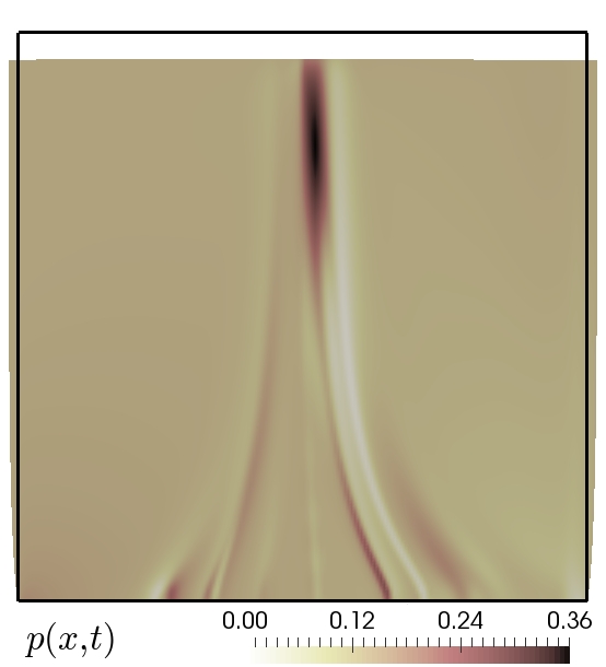
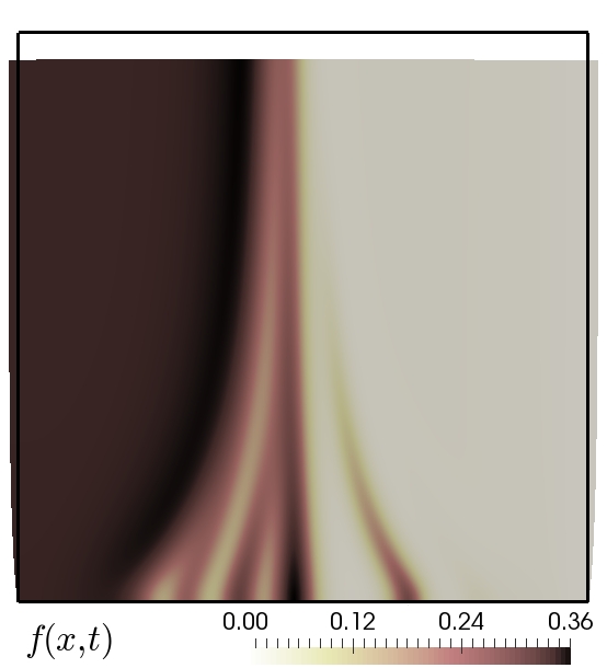
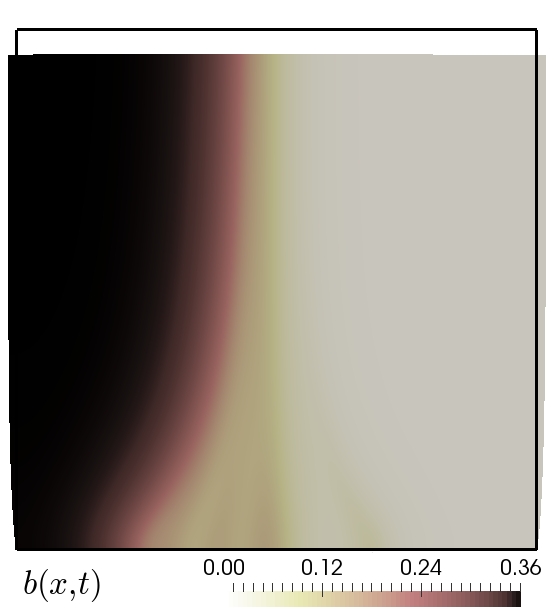
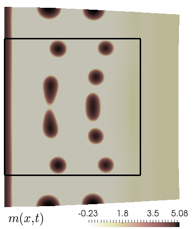
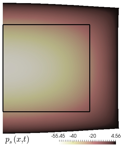
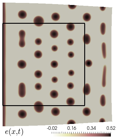
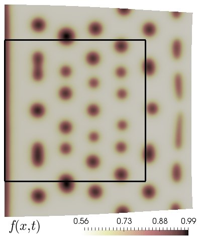
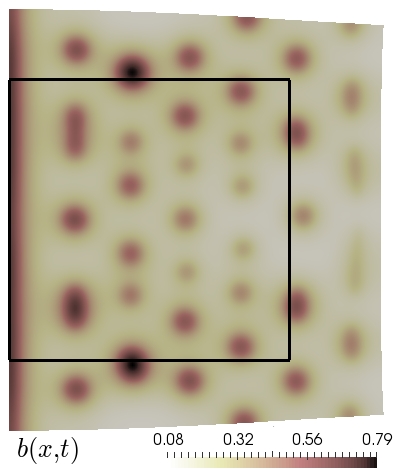
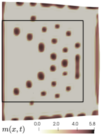
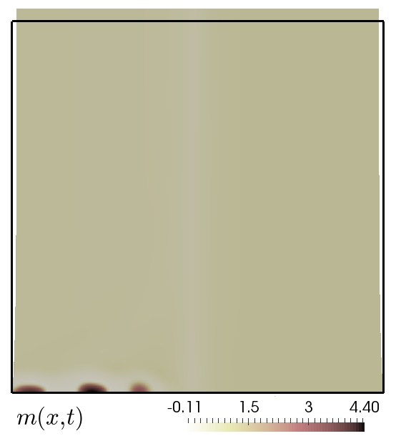
Figure 5.2: Evolution of the mesenchymal cell concentration at t=160,280,400,520𝑡160280400520t=160,280,400,520 under periodic traction applied on the top edge of the domain (top); and snapshots of fluid pressure, epithelium, FGF, and BMP at t=520𝑡520t=520 (bottom row).

5.3 Suppressed solid motion vs. periodic boundary traction.

In order to emphasise the effect of the stretch and deformation on the formation of patterns we compare the concentration of mesenchymal cells in two cases, one where the motion of the domain is suppressed (by setting τ=0𝜏0\tau=0), and another scenario where the bottom of the domain, (Γ)Γ(\Gamma), is kept clamped, the top of the domain undergoes a (relatively small) periodic traction, and the vertical faces are kept with zero traction. In this case we employ the linear poroelastic model from Section 2, and a zero fluid pressure flux is imposed on Σ=ΩΓΣΩΓ\Sigma=\partial\Omega\setminus\Gamma. The spatial domain is a square Ω=(0,20)2Ωsuperscript0202\Omega=(0,20)^{2} discretised into 58482 triangular elements, and the model parameters that are modified with respect to those in Table 1 adopt the values

m0=0.75,Dm=0.03,τ=ξf=0.001.formulae-sequencesubscript𝑚00.75formulae-sequencesubscript𝐷𝑚0.03𝜏subscript𝜉𝑓0.001m_{0}=0.75,\quad D_{m}=0.03,\quad\tau=\xi_{f}=0.001.

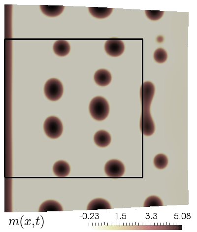
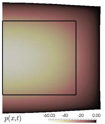
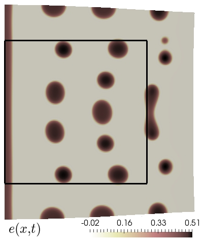
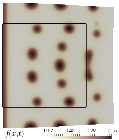
The traction is 𝒕=(0,s0sin(πt/t^))𝒕superscript0subscript𝑠0𝜋𝑡^𝑡\boldsymbol{t}=(0,s_{0}\sin(\pi t/\hat{t}))^{\intercal}, with magnitude s0=1500subscript𝑠01500s_{0}=1500 and period t^=320^𝑡320\hat{t}=320. We employ a fixed time step Δt=0.2Δ𝑡0.2\Delta t=0.2 and advance the system until t=520𝑡520t=520. The outcome of these tests is collected in Figure 5.1 and Figure 5.2, where we observed that slight modifications in the poromechanics result in quite drastic alterations of the clustering of mesenchymal cells. For instance, in Figure 5.2 we see that on the bottom edge of the domain (where displacements are zero during the whole simulation), the relatively large stretches applied elsewhere on the body do not break the formation of dotted-shaped patterns at early stages, but they are swept away as time advances.
Refer to caption
Refer to caption
Refer to caption
Refer to caption
Refer to caption
Refer to caption
Refer to caption
Refer to caption
Refer to caption
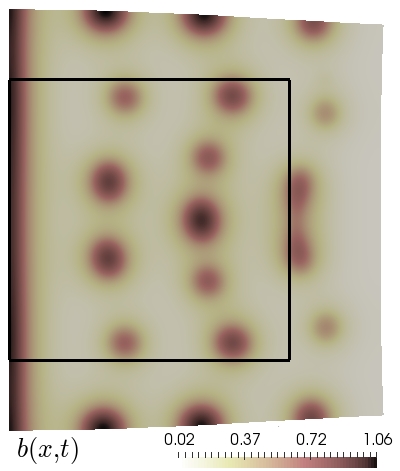
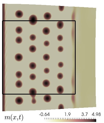
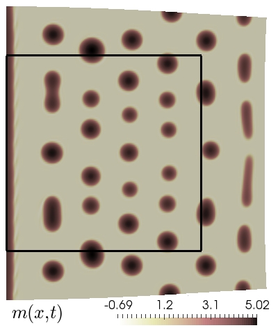
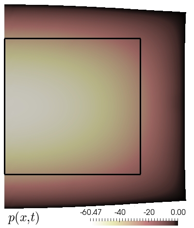
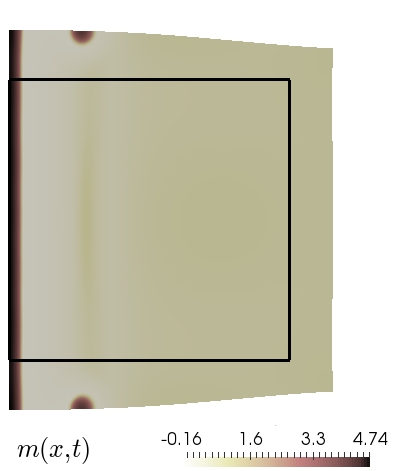
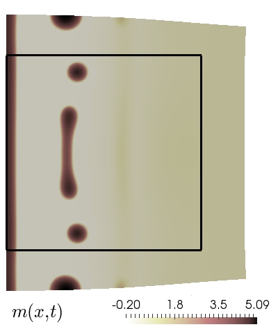
Figure 5.3: Evolution of the mesenchymal cell concentration under finite growth using the formulation (4.14), snapshots are taken at t=160,280,400,520𝑡160280400520t=160,280,400,520 (first row). Bottom: plots at t=520𝑡520t=520 of fluid pressure, solid pressure, epithelium, FGF, and BMP. Mechano-chemical coupling governed by ξf=0.5subscript𝜉𝑓0.5\xi_{f}=0.5.

5.4 Finite growth in 2D.

Next we maintain the domain and most model parameters as in the previous case and focus on the coupled model defined in Section 4. Determining the total first Piola-Kirchhoff stress from (4.11) and the growth specification (4.14) (with δ2=0.15subscript𝛿20.15\delta_{2}=0.15, δ3=0.045subscript𝛿30.045\delta_{3}=0.045), we modify also the boundary treatment and consider that Γ0subscriptΓ0\Gamma_{0} is the left edge of the domain whereas the remainder of Ω0subscriptΩ0\partial\Omega_{0} is Σ0subscriptΣ0\Sigma_{0}. On Γ0subscriptΓ0\Gamma_{0} we impose zero normal displacement 𝒖𝐍0=0𝒖subscript𝐍00\boldsymbol{u}\cdot\mathbf{N}_{0}=0 and a Robin boundary condition with constant ξR=0.0001subscript𝜉𝑅0.0001\xi_{R}=0.0001 is set on Σ0subscriptΣ0\Sigma_{0}. The shear modulus is μ=4𝜇4\mu=4, the solid permeability is augmented to κ=0.001𝜅0.001\kappa=0.001, and we take ξf=0.3subscript𝜉𝑓0.3\xi_{f}=0.3. The fluid mass source is specified by (4.15) with 0=0.001subscript00.001\ell_{0}=0.001.

The panels in Figure 5.3 display transients of the growth of the initial domain and we plot the concentration of mesenchymal cells on the deformed configuration. We can observe that the patterns follow a different alignment than those formed in Figure 5.1, in particular disrupting the symmetry and the size distribution of the dotted-shaped patterns. The plots in the bottom row show the fluid and solid pressure together with the remaining chemical concentrations at the final time. Note that both solid and fluid pressures accumulate near Σ0subscriptΣ0\Sigma_{0}. In addition, we note that the values of FGF at later times are negative since the last term on the left-hand side of (4.17c) represents a sink of f𝑓f as the domain only grows (and tr𝐂dtr𝐂𝑑\mathop{\mathrm{tr}}\nolimits\mathbf{C}-d is non-negative) throughout the simulation. We then change the sign of ξf=0.3subscript𝜉𝑓0.3\xi_{f}=-0.3 and obtain positive FGF concentrations as well as similar patterns in all fields (but exhibiting a higher wave-number than in the previous case). The results from these tests are shown in Figure 5.4.

Refer to caption
Refer to caption
Refer to caption
Refer to caption
Refer to caption
Refer to caption
Refer to caption
Refer to caption
Refer to caption
Figure 5.4: Evolution of the mesenchymal cell concentration under finite growth using the formulation (4.14), snapshots are taken at t=160,280,400,520𝑡160280400520t=160,280,400,520 (top). Second row: plots at t=520𝑡520t=520 of fluid pressure, solid pressure, epithelium, FGF, and BMP. Simulations using ξf=0.5subscript𝜉𝑓0.5\xi_{f}=-0.5.

5.5 Finite growth in 3D.

To close this section we proceed to extend the previous example to the 3D case. The undeformed domain is still a simple geometry Ω0=(0,20)×(0,20)×(0,1)subscriptΩ002002001\Omega_{0}=(0,20)\times(0,20)\times(0,1), where to obtain an accurate solution we used 140 elements per side in the X1subscript𝑋1X_{1} and X2subscript𝑋2X_{2} directions, and instead considered only 8 in the X3subscript𝑋3X_{3} direction. This results in roughly 10 million degrees of freedom. The sides at X1=0subscript𝑋10X_{1}=0 and X3=0subscript𝑋30X_{3}=0 constitute Γ0subscriptΓ0\Gamma_{0}, where zero normal displacements are considered, and on the remainder of the boundary we set Robin conditions as above, but using ξR=0.001subscript𝜉𝑅0.001\xi_{R}=0.001. The growth factors are considered as in (4.13) with the specification δ1=1/52subscript𝛿1152\delta_{1}=1/52, δ2=0subscript𝛿20\delta_{2}=0, δ3=1/104subscript𝛿31104\delta_{3}=1/104. The results are shown in Figure 5.5, where we plot the evolution of the chemicals in the deformed configuration, and where the outline of the undeformed domain is also shown for visualisation purposes. We can see that as time progresses, the transversally isotropic growth depending only on time occurs mainly in the plane X1X2subscript𝑋1subscript𝑋2X_{1}X_{2} as in the 2D case. Most interestingly, the mesenchymal concentration exhibits new complex structures. From the upper view, an arrow-like structure can be seen, where from higher concentrations appear more distant when going from right to left. From the slice view below, it can be seen how these distant concentrations are instead connected within the geometry, and we stress that this type of patterns can only be described by the 3D model. Still, these patterns are not representative of the actual primordial patterns, which are composed by independent buds, so this aspect still requires further investigation.
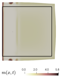
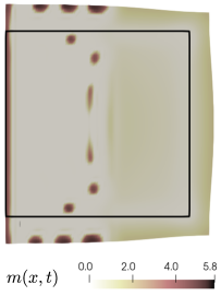
Refer to caption
Refer to caption
Refer to caption
Refer to caption
Refer to caption
Refer to caption
Refer to caption
Refer to caption
Refer to caption
Refer to caption
Figure 5.5: Evolution of the mesenchymal cell concentration under finite growth using the formulation (4.13), snapshots are taken at t=160,280,400,520𝑡160280400520t=160,280,400,520 (top). We also display the fluid and solid pressures (second row), the mesenchymal and epithelium concentrations (third row), and the FGF and BMP (fourth row).

6 Concluding remarks

We have proposed a model for describing the interaction between poroelastic deformations and chemotactical displacement of mesenchymal cells, FGF, BMP and epithelium. In the regime of small strains, the coupling mechanisms include degradation of FGF due to local solid compression, advection of chemicals through solid velocity, and an active stress driven by mesenchymal cells. We have derived a set of conditions for Turing patterns to emerge, focusing on the two-way coupling and the main coupling variables. We have proposed an extended model that accounts for growth and hyperelastic deformations of the solid matrix, and the coupling mechanisms in this case consist in intrinsic growth functions depending on time and on the concentration of mesenchymal cells, as well as modification of the diffusion coefficients in the chemotaxis model due to changes from spatial to reference coordinates.

The linear stability analysis for the nonlinearly coupled system from Section 4 could be carried out extending our results from Section 3 following the ideas from [6]. As the main application is on skin patterning for feather development, we could also incorporate growth models specifically targeted for shells or thin plates as in [14], and concentrate on bi-layered structures extending the formulations in [13].

Acknowledgements

This research was funded by the Monash Mathematics Research Fund S05802-3951284; and by the Australian Research Council through the Discovery Project grant DP220103160.

Appendix

Proof of Proposition 3.1.

The spatial derivatives in the scalar case follow trivially from the definition of f𝑓f. Both scalar and vector time derivatives also follow directly from the definition of f,𝒗𝑓𝒗f,\boldsymbol{v}. For the spatial derivatives of 𝒗𝒗\boldsymbol{v}, using the definition of the differential operators and denoting {𝐞^n}1,,dsubscriptsubscript^𝐞𝑛1𝑑\{\widehat{\mathrm{\boldsymbol{e}}}_{n}\}_{1,\ldots,d}, the standard basis vectors in dsuperscript𝑑\mathbb{R}^{d}, we can readily write

div𝒗div𝒗\displaystyle\mathop{\mathrm{div}}\nolimits\boldsymbol{v} =nxnvn,0ei𝒌𝒙+ϕt=niknvn,0ei𝒌𝒙+ϕt=niknvn=i𝒗𝒌,absentsubscript𝑛subscriptsubscript𝑥𝑛subscript𝑣𝑛0superscriptei𝒌𝒙italic-ϕ𝑡subscript𝑛isubscript𝑘𝑛subscript𝑣𝑛0superscriptei𝒌𝒙italic-ϕ𝑡subscript𝑛isubscript𝑘𝑛subscript𝑣𝑛i𝒗𝒌\displaystyle=\sum_{n}\partial_{x_{n}}v_{n,0}\mathrm{e}^{\mathrm{i}\boldsymbol{k}\cdot\boldsymbol{x}+\phi t}=\sum_{n}\mathrm{i}k_{n}v_{n,0}\mathrm{e}^{\mathrm{i}\boldsymbol{k}\cdot\boldsymbol{x}+\phi t}=\sum_{n}\mathrm{i}k_{n}v_{n}=\mathrm{i}\boldsymbol{v}\cdot\boldsymbol{k},
𝒗bold-∇𝒗\displaystyle\boldsymbol{\nabla}\boldsymbol{v} =mxm𝒗𝐞^m=n,mxmvn,0ei𝒌𝒙+ϕt𝐞^n𝐞^m=n,mikmvn,0ei𝒌𝒙+ϕt𝐞^n𝐞^mabsentsubscript𝑚subscriptsubscript𝑥𝑚tensor-product𝒗subscript^𝐞𝑚subscript𝑛𝑚subscriptsubscript𝑥𝑚tensor-productsubscript𝑣𝑛0superscriptei𝒌𝒙italic-ϕ𝑡subscript^𝐞𝑛subscript^𝐞𝑚subscript𝑛𝑚tensor-productisubscript𝑘𝑚subscript𝑣𝑛0superscriptei𝒌𝒙italic-ϕ𝑡subscript^𝐞𝑛subscript^𝐞𝑚\displaystyle=\sum_{m}\partial_{x_{m}}\boldsymbol{v}\otimes\widehat{\mathrm{\boldsymbol{e}}}_{m}=\sum_{n,m}\partial_{x_{m}}v_{n,0}\mathrm{e}^{\mathrm{i}\boldsymbol{k}\cdot\boldsymbol{x}+\phi t}\widehat{\mathrm{\boldsymbol{e}}}_{n}\otimes\widehat{\mathrm{\boldsymbol{e}}}_{m}=\sum_{n,m}\mathrm{i}k_{m}v_{n,0}\mathrm{e}^{\mathrm{i}\boldsymbol{k}\cdot\boldsymbol{x}+\phi t}\widehat{\mathrm{\boldsymbol{e}}}_{n}\otimes\widehat{\mathrm{\boldsymbol{e}}}_{m}
=n,mikmvn𝐞^n𝐞^m=mikm𝒗𝐞^m=i𝒗𝒌.absentsubscript𝑛𝑚tensor-productisubscript𝑘𝑚subscript𝑣𝑛subscript^𝐞𝑛subscript^𝐞𝑚subscript𝑚tensor-productisubscript𝑘𝑚𝒗subscript^𝐞𝑚tensor-producti𝒗𝒌\displaystyle=\sum_{n,m}\mathrm{i}k_{m}v_{n}\widehat{\mathrm{\boldsymbol{e}}}_{n}\otimes\widehat{\mathrm{\boldsymbol{e}}}_{m}=\sum_{m}\mathrm{i}k_{m}\boldsymbol{v}\otimes\widehat{\mathrm{\boldsymbol{e}}}_{m}=\mathrm{i}\boldsymbol{v}\otimes\boldsymbol{k}.

On the other hand, using (3.2a) we can then straightforwardly derive (3.2b) as follows

𝐝𝐢𝐯𝜺(𝒗)𝐝𝐢𝐯𝜺𝒗\displaystyle\mathop{\mathbf{div}}\nolimits\boldsymbol{\varepsilon}(\boldsymbol{v}) =𝐝𝐢𝐯(n,mivnkm+vmkn2𝐞^n𝐞^m)=n,mi2vnknkm+vmkn22𝐞^mabsent𝐝𝐢𝐯subscript𝑛𝑚tensor-productisubscript𝑣𝑛subscript𝑘𝑚subscript𝑣𝑚subscript𝑘𝑛2subscript^𝐞𝑛subscript^𝐞𝑚subscript𝑛𝑚superscripti2subscript𝑣𝑛subscript𝑘𝑛subscript𝑘𝑚subscript𝑣𝑚superscriptsubscript𝑘𝑛22subscript^𝐞𝑚\displaystyle=\mathop{\mathbf{div}}\nolimits\left(\sum_{n,m}\mathrm{i}\frac{v_{n}k_{m}+v_{m}k_{n}}{2}\widehat{\mathrm{\boldsymbol{e}}}_{n}\otimes\widehat{\mathrm{\boldsymbol{e}}}_{m}\right)=\sum_{n,m}\mathrm{i}^{2}\frac{v_{n}k_{n}k_{m}+v_{m}k_{n}^{2}}{2}\widehat{\mathrm{\boldsymbol{e}}}_{m}
=12m(𝒗𝒌)km𝐞^m+k2vm𝐞^m=(𝒗𝒌)𝒌+k2𝒗2,absent12subscript𝑚𝒗𝒌subscript𝑘𝑚subscript^𝐞𝑚superscript𝑘2subscript𝑣𝑚subscript^𝐞𝑚𝒗𝒌𝒌superscript𝑘2𝒗2\displaystyle=-\frac{1}{2}\sum_{m}(\boldsymbol{v}\cdot\boldsymbol{k})k_{m}\widehat{\mathrm{\boldsymbol{e}}}_{m}+k^{2}v_{m}\widehat{\mathrm{\boldsymbol{e}}}_{m}=-\frac{(\boldsymbol{v}\cdot\boldsymbol{k})\boldsymbol{k}+k^{2}\boldsymbol{v}}{2},
t𝜺(𝒗)subscript𝑡𝜺𝒗\displaystyle\partial_{t}\boldsymbol{\varepsilon}(\boldsymbol{v}) =(12(t𝒗+t𝒗))=(ϕ2(𝒗+𝒗))=ϕ𝜺(𝒗),absent12bold-∇subscript𝑡𝒗bold-∇subscript𝑡superscript𝒗italic-ϕ2bold-∇𝒗bold-∇superscript𝒗italic-ϕ𝜺𝒗\displaystyle=\left(\frac{1}{2}(\boldsymbol{\nabla}\partial_{t}\boldsymbol{v}+\boldsymbol{\nabla}\partial_{t}\boldsymbol{v}^{\intercal})\right)=\left(\frac{\phi}{2}(\boldsymbol{\nabla}\boldsymbol{v}+\boldsymbol{\nabla}\boldsymbol{v}^{\intercal})\right)=\phi\boldsymbol{\varepsilon}(\boldsymbol{v}),
𝐝𝐢𝐯(θ𝐈)𝐝𝐢𝐯𝜃𝐈\displaystyle\mathop{\mathbf{div}}\nolimits(\theta\mathbf{I}) =θ=(i𝒗𝒌)=inxn(𝒗𝒌)𝐞^n=in,mkmxnvm𝐞^n=i2n,mkmknvm𝐞^nabsent𝜃i𝒗𝒌isubscript𝑛subscriptsubscript𝑥𝑛𝒗𝒌subscript^𝐞𝑛isubscript𝑛𝑚subscript𝑘𝑚subscriptsubscript𝑥𝑛subscript𝑣𝑚subscript^𝐞𝑛superscripti2subscript𝑛𝑚subscript𝑘𝑚subscript𝑘𝑛subscript𝑣𝑚subscript^𝐞𝑛\displaystyle=\nabla\theta=\nabla(\mathrm{i}\boldsymbol{v}\cdot\boldsymbol{k})=\mathrm{i}\sum_{n}\partial_{x_{n}}(\boldsymbol{v}\cdot\boldsymbol{k})\widehat{\mathrm{\boldsymbol{e}}}_{n}=\mathrm{i}\sum_{n,m}k_{m}\partial_{x_{n}}v_{m}\widehat{\mathrm{\boldsymbol{e}}}_{n}=\mathrm{i}^{2}\sum_{n,m}k_{m}k_{n}v_{m}\widehat{\mathrm{\boldsymbol{e}}}_{n}
=nkn(𝒗𝒌)𝐞^n=(𝒗𝒌)𝒌,absentsubscript𝑛subscript𝑘𝑛𝒗𝒌subscript^𝐞𝑛𝒗𝒌𝒌\displaystyle=-\sum_{n}k_{n}(\boldsymbol{v}\cdot\boldsymbol{k})\widehat{\mathrm{\boldsymbol{e}}}_{n}=-(\boldsymbol{v}\cdot\boldsymbol{k})\boldsymbol{k},
tθsubscript𝑡𝜃\displaystyle\partial_{t}\theta =divt𝒗=ϕdiv𝒗=ϕθ.absentdivsubscript𝑡𝒗italic-ϕdiv𝒗italic-ϕ𝜃\displaystyle=\mathop{\mathrm{div}}\nolimits\partial_{t}\boldsymbol{v}=\phi\mathop{\mathrm{div}}\nolimits\boldsymbol{v}=\phi\theta.

References

  • [1] M.S. Alnæs, J. Blechta, J. Hake, A. Johansson, B. Kehlet, A. Logg, C. Richardson, J. Ring, M.E. Rognes, and G.N. Wells, The FEniCS project version 1.5. Arch. Numer. Softw., 3(100) (2015) 9–23.
  • [2] N. Barnafi, S. Di Gregorio, L. Dedè, P. Zunino, C. Vergara, and A. Quarteroni, A multiscale poromechanics model integrating myocardial perfusion and systemic circulation. SIAM J. Appl. Math., 82(4) (2021) 1113–1660.
  • [3] N. Barnafi, B. Gómez-Vargas, W.J. Lourenço, R.F. Reis, B.M. Rocha, M. Lobosco, R. Ruiz-Baier, and R. Weber dos Santos, Finite element methods for large-strain poroelasticity/chemotaxis models simulating the formation of myocardial oedema. J. Sci. Comput., 92 (2022) e92(1–40).
  • [4] N. Barnafi, P. Zunino, L. Dedè, and A. Quarteroni, Mathematical analysis and numerical approximation of a general linearized poro-hyperelastic model. Comput. Math. Appl., 91 (2021) 202–228.
  • [5] M. Borregales, F.A. Radu, K. Kumar, and J.M. Nordbotten, Robust iterative schemes for non-linear poromechanics. Computat. Geosci., 22 (2018) 1021–1038.
  • [6] M. Ben Amar and A. Goriely, Growth and instability in elastic tissues. J. Mech. Phys. Solids, 53 (2005) 2284–2319.
  • [7] L. Berger, R. Bordas, K. Burrowes, V. Grau, S. Tavener, D. Kay, A poroelastic model coupled to a fluid network with applications in lung modelling. Int. J. Numer. Meth. Bio., 32(1) (2016) e02731.
  • [8] L. Berger, R. Bordas, D. Kay, and S. Tavener, A stabilized finite element method for finite-strain three-field poroelasticity. Comput. Mech., 60(1) (2017) 51–68.
  • [9] D. Braess and P. Ming, A finite element method for nearly incompressible elasticity problems. Math. Comp., 74 (2005) 25–52.
  • [10] D. Chapelle, J.-F. Gerbeau, J. Sainte-Marie, and I.E. Vignon-Clementel, A poroelastic model valid in large strains with applications to perfusion in cardiac modeling. Comput. Mech., 46 (2010) 91–101.
  • [11] J. Collis, D.L. Brown, M.E. Hubbard, and R.D. O’Dea, Effective equations governing an active poroelastic medium. Proc. R. Soc. A, 473 (2017) e20160755.
  • [12] O. Coussy, Poromechanics. John Wiley & Sons, (2004).
  • [13] L.M. De Oliveira Vilaca, M.C. Milinkovitch, and R. Ruiz-Baier, Numerical approximation of a 3D mechanochemical interface model for skin patterning. J. Comput. Phys., 384 (2019) 283–404.
  • [14] J. Dervaux, P. Ciarletta, and M. Ben Amar, Morphogenesis of thin hyperelastic plates: A constitutive theory of biological growth in the Föppl–von Kármaán limit. J. Mech. Phys. Solids, 57 (2009) 458–471.
  • [15] F. Rathgeber, D.A. Ham, L. Mitchell, M. Lange, F. Luporini, A.T.T. McRae, G.T. Bercea, G.R. Markall, and P.H.J. Kelly, Firedrake: automating the finite element method by composing abstractions. ACM T. Math. Software (TOMS), 43 (2016), 1–27.
  • [16] C. Giverso, M. Scianna, and A. Grillo, Growing avascular tumours as elastoplastic bodies by the theory of evolving natural configurations. Mech. Res. Comm., 68 (2015), 31–39.
  • [17] J.D. Glover, K.L. Wells, F. Matthäus, K.J. Painter, W. Ho, J. Riddell, J.A. Johansson, M.J. Ford, C.A.B. Jahoda, V. Klika, R.L. Mort, and D.J. Headon, Hierarchical patterning modes orchestrate hair follicle morphogenesis. PLOS Bio., 15(7) (2007) 1–31.
  • [18] J. Guiu-Souto and A. P. Munuzuri, Influence of oscillatory centrifugal forces on the mechanism of Turing pattern formation, Phys. Rev. E, 91(1) (2015) e012917.
  • [19] M. Hine Armstrong, A. Buganza Tepole, E. Kuhl, B.R. Simon, and J.P. Vande Geest, A finite element model for mixed porohyperelasticity with transport, swelling, and growth. PLOS One, 11(4) (2016) e0152806.
  • [20] W.K.W. Ho, L. Freem, D. Zhao, K.J. Painter, T.E. Woolley, E.A. Gaffney, M.J. McGrew, A. Tzika, M. Milinkovitch, P. Schneider, A. Drusko, F. Matthäus, J.L. Glover, K.L. Wells, J.A. Johansson, M.G. Davey, H.M. Sang, M. Clinton, and D.J. Headon, Feather arrays are patterned by interacting signalling and cell density waves. PLOS Bio., 17(2) (2019) e3000132.
  • [21] R.S. Dembo, S.C Eisenstat, and T. Steihaug, Inexact Newton methods. SIAM J. Numer. anal., 19(2) (1982) 400-408.
  • [22] G.W. Jones and S.J. Chapman, Modeling growth in biological materials. SIAM Rev., 54(1) (2012) 52–118.
  • [23] N. Kida and Y. Morishita, Continuum mechanical modeling of developing epithelial tissues withanisotropic surface growth. Finite Element Anal. Design, 144 (2018) 49–60.
  • [24] E.F. Keller and L.A. Segel, Initiation of slime mold aggregation viewed as an instability. J. Theor. Biol., 26(3) (1970) 399-415.
  • [25] E. Kuhl, Growing matter: a review of growth in living systems. J. Mech. Behav. Biomed. Mater., 29 (2014) 529–543.
  • [26] E.H. Lee, Elastic-plastic deformation at finite strains. J. Appl. Mech., 36(1) (1969) 1–6.
  • [27] C.M. Lin, T.X. Jiang, R.E. Baker, P.K. Maini, R.B. Widelitz, and C.M. Chuong, Spots and stripes: pleomorphic patterning of stem cells via p-ERK-dependent cell chemotaxis shown by feather morphogenesis and mathematical simulation. Dev. Biol., 334(2) (2009) 369–382.
  • [28] W.d.J. Lourenço, R.F. Reis, R. Ruiz-Baier, B.M. Rocha, R. Weber dos Santos, and M. Lobosco, A poroelastic approach for modelling myocardial oedema in acute myocarditis, Frontiers Physiol., 13 (2022) e888515(1–14).
  • [29] C.W. MacMinn, E.R. Dufresne, and J.S. Wettlaufer, Large deformations of a soft porous material. Phys. Rev. Appl., 5 (2016) e044020.
  • [30] P. Mascheroni, M. Carfagna, A. Grillo, D.P. Boso, and B.A. Schrefler, An avascular tumor growth model based on porous media mechanics and evolving natural states. Math. Mech. Solids, 23 (2018) 686–712.
  • [31] E. Moeendarbary, L. Valon, M. Fritzsche, A.R. Harris, D.A. Moulding, A.J. Thrasher, E. Stride, L. Mahadevan, and G.T. Charras, The cytoplasm of living cells behaves as a poroelastic material. Nature Materials, 12 (2013) e3517.
  • [32] P. Moreo, E.A. Gaffney, J.M. García-Aznar, and M. Doblaré, On the modelling of biological patterns with mechanochemical models: Insights from analysis and computation. Bull. Math. Biol., 72 (2010) 400–431.
  • [33] C. Mou, F. Pitel, D. Gourichon, F. Vignoles, A. Tzika, P. Tato, L. Yu, D.W. Burt, B. Bed’Hom, M. Tixier-Boichard, K.J. Painter, D.J. Headon, Cryptic patterning of avian skin confers a developmental facility for loss of neck feathering. PLoS Biol., 9(3) (2011) e1001028.
  • [34] J.D. Murray, P.K. Maini, and R.T. Tranquillo, Mechanochemical models for generating biological pattern and form in development. Phys. Reports, 171(2) (1988) 59–84.
  • [35] K.J. Painter, G.S. Hunt, K.L. Wells, J.A. Johansson, and D.J. Headon, Towards an integrated experimental–theoretical approach for assessing the mechanistic basis of hair and feather morphogenesis. Interface Focus, 2(4) (2012) 433-450.
  • [36] K.J. Painter, W. Ho, and D.J. Headon, A chemotaxis model of feather primordia pattern formation during avian development. J. Theor. Biol., 437 (2018) 225–238.
  • [37] R. Penta, D. Ambrosi, and R.J. Shipley, Effective governing equations for poroelastic growing media. Q. J. Mech. Appl. Math., 67 (2014) 69–91.
  • [38] P. Recho, A. Hallou, and E. Hannezo, Theory of mechano-chemical pattering in biphasic biological tissues. PNAS, 116(12) (2019) 5344–5349.
  • [39] E.K. Rodriguez, A. Hoger, and A.D. McCulloch, Stress-dependent finite growth in soft elastic tissues. J. Biomech., 27 (4) (1994) 455–467.
  • [40] E.J. Routh, A Treatise on the Stability of a Given State of Motion: Particularly Steady Motion. Macmillan and Company, London (1877).
  • [41] R. Sacco, P. Causin, C. Lelli, and M.T. Raimondi, A poroelastic mixture model of mechanobiological processes in biomass growth: theory and application to tissue engineering. Meccanica, 52(14) (2017) 3273–3297.
  • [42] R.E. Showalter, Diffusion in poro-elastic media. J. Math. Anal. Appl., 251 (2000) 310–340.
  • [43] L. Socci, G. Pennati, F. Gervaso, and P. Vena, An axisymmetric computational model of skin expansion and growth. Biomech. Model. Mechanobiol., 6(3) (2007) 177–188.
  • [44] A. Tosin, Mechanics and chemotaxis in the morphogenesis of vascular networks. B. Math. Biol., 68(7) (2006) 1819–1836.
  • [45] N. Verma, B. Gómez-Vargas, L. M. De Oliveira Vilaca, S. Kumar, and R. Ruiz-Baier, Well-posedness and discrete analysis for advection-diffusion-reaction in poroelastic media. Applic. Analysis, 101(14) (2022) 4914–4941.
  • [46] L.M.D.O. Vilaca, B. Gómez-Vargas, S. Kumar, R. Ruiz-Baier, and N. Verma, Stability analysis for a new model of multi-species convection-diffusion-reaction in poroelastic tissue. Appl. Math. Model., 84 (2020) 425–446.
  • [47] A.-T. Vuong, L. Yoshihara, and W.A. Wall, A general approach for modeling nteracting flow through porous media under finite deformations. Comput. Methods Appl. Mech. Engrg., 283 (2015) 1240–1259.
  • [48] X. Yang, D. Dormann, A.E. Münsterberg, and C.J. Weijer, Cell movement patterns during gastrulation in the chick are controlled by positive and negative chemotaxis mediated by FGF4 and FGF8. Dev. Cell, 3(3) (2002) 425–437.