\jyear

2022

[1]\fnmXiaolin \surHuang

1]\orgdivInstitute of Image Processing and Pattern Recognition, \orgnameShanghai Jiao Tong University, \orgaddress\street800 Dongchuan RD. Minhang District, \cityShanghai, \postcode200240, \countryChina

2]\orgdivLaboratory for Information and Inference Systems, \orgnameÉcole Polytechnique Fédérale de Lausanne, \orgaddress\streetEPFL SV-BMC AA-B118, \cityLausanne, \postcode1015, \countrySwitzerland

Random Fourier Features for Asymmetric kernels

\fnmMingzhen \surHe mingzhen_he@sjtu.edu.cn    \fnmFan \surHe hf-inspire@sjtu.edu.cn    \fnmFanghui \surLiu fanghui.liu@epfl.ch    xiaolinhuang@sjtu.edu.cn [ [
Abstract

The random Fourier features (RFFs) method is a powerful and popular technique in kernel approximation for scalability of kernel methods. The theoretical foundation of RFFs is based on the Bochner theorem (Bochner,, 2005) that relates symmetric, positive definite (PD) functions to probability measures. This condition naturally excludes asymmetric functions with a wide range applications in practice, e.g., directed graphs, conditional probability, and asymmetric kernels. Nevertheless, understanding asymmetric functions (kernels) and its scalability via RFFs is unclear both theoretically and empirically. In this paper, we introduce a complex measure with the real and imaginary parts corresponding to four finite positive measures, which expands the application scope of the Bochner theorem. By doing so, this framework allows for handling classical symmetric, PD kernels via one positive measure; symmetric, non-positive definite kernels via signed measures; and asymmetric kernels via complex measures, thereby unifying them into a general framework by RFFs, named AsK-RFFs. Such approximation scheme via complex measures enjoys theoretical guarantees in the perspective of the uniform convergence. In algorithmic implementation, to speed up the kernel approximation process, which is expensive due to the calculation of total mass, we employ a subset-based fast estimation method that optimizes total masses on a sub-training set, which enjoys computational efficiency in high dimensions. Our AsK-RFFs method is empirically validated on several typical large-scale datasets and achieves promising kernel approximation performance, which demonstrate the effectiveness of AsK-RFFs.

keywords:
Kernel approximation, random Fourier features, asymmetric kernels, convergence bounds

1 Introduction

Kernel methods (Schölkopf and Smola,, 2002; Suykens et al.,, 2002; Vapnik,, 2013) play a significant role in statistical machine learning in almost all the topics, e.g., classification (Soman et al.,, 2009), regression (Drucker et al.,, 1997), clustering (Girolami,, 2002), and dimension reduction (Schölkopf et al.,, 1997). One significant limitation is the lack of scalability due to the fact that kernel methods are working on the kernel matrices which have the size N×N𝑁𝑁N\times N with N𝑁N being the number of samples. Kernel approximation (Williams and Seeger,, 2001; Drineas et al.,, 2005; Liu et al., 2021b, ) is able to address this issue by approximating the original kernel matrix or kernel function. One typical technique tool is Random Fourier features (RFFs) that introduces low dimensional randomized feature mappings for approximating the original kernel function (Rahimi and Recht,, 2007, 2008). The theoretical foundation of RFFs is established by the Bochner’s theorem in harmonic analysis (Bochner,, 2005; Rahimi and Recht,, 2007). The Bochner’s theorem claims that a continuous, symmetric, shift-invariant and positive definite (PD) function can be approximated by a finite non-negative measure. Besides, RFFs can be regarded as a two-layer neural network with only training the second layer, which naturally bridges kernel methods and neural networks in deep learning theory (Mehrkanoon and Suykens,, 2018; Belkin et al.,, 2019; Malach et al.,, 2020); refer to one recent survey (Liu et al., 2021b, ).

The target of RFFs is to establish an explicit feature mapping via the sampled random features and then approximate the original kernel function via inner product. There is a strict pre-condition on RFFs that the sampling measure is well-defined only when the kernel is stationary, PD, and symmetric. Extension of RFFs to other kernels, e.g., polynomial kernels (Pennington et al.,, 2015), non-positive definite kernel, e.g., the neural tangent kernel of two-layer ReLU networks with unit spherical constraints (Liu et al., 2021a, ) is important and has been discussed. However, study on RFFs for asymmetric kernels is missing in the machine learning community.

In practice, asymmetric similarities/dissimilarities are commonly used. Here we take several typical examples to illustrate this. 1) In directed graphs, the adjacency matrices that record (weighted) connections between two samples can efficiently represent asymmetric similarities. The relationship between a central and a local node can be asymmetric. For example, in federated learning, the central update is aggregated by updates of all local nodes. In this case, neural tangent kernel-based federated learning is asymmetric (Huang et al.,, 2021). 2) the conditional probability is another popular scene we may meet asymmetric similarities due to P(A|B)P(B|A)Pconditional𝐴𝐵Pconditional𝐵𝐴{\rm P}(A|B)\neq{\rm P}(B|A) in general, where A𝐴A and B𝐵B are two events in an event space. Some applications for conditional probabilities could be found in the works of Hinton and Roweis, (2002); Tang et al., 2015a ; Tang et al., 2015b . 3) Asymmetric kernels, as a tool more flexible than PD kernels, are promising to connect to deep models. As an encouraging attempt, Wright and Gonzalez, (2021) successfully characterize the dot-product attention by asymmetric kernels and provides a theoretical understanding of transformer models (Vaswani et al.,, 2017).

In theory, the function space associated with asymmetric kernels is often built on reproducing kernel Banach spaces (RKBS) (Zhang et al.,, 2009; Song et al.,, 2013; Fasshauer et al.,, 2015; Bartolucci et al.,, 2021; Lin et al.,, 2022) instead of the classical reproducing kernel Hilbert spaces (RKHS). For the primal feature analysis, Suykens, (2016, 2017) introduce a variational principle for understanding the singular value decomposition from the perspective of asymmetric kernels associated with different feature mappings. These theories are helpful for understanding asymmetric kernels but are not suitable to handle the approximation problem.

Extension of standard RFFs to asymmetric kernels is unanswered and non-trivial both theoretically and algorithmically. To be specific, theoretically, the original probability measure for PD kernels (Rahimi and Recht,, 2007) and signed measure for indefinite but symmetric kernels (Huang et al.,, 2017; Liu et al., 2021a, ) cannot be used as the sampling measure for asymmetric kernels, which is the main obstacle of RFFs for asymmetric kernels. Algorithmically, the point evaluation at the origin is not sufficient to represent the corresponding total masses of measures, which differs from that in the Bochner’s theorem. In this scene, calculation of total masses often involves a d𝑑d dimensional numerical integral, which is time-consuming in high dimensions.

In this paper, we propose a unified kernel approximation framework for asymmetric kernels by RFFs, called AsK-RFFs, which fills the gap of asymmetric kernels from theory to practice. Ask-RFFs design a complex measure on the sample space for a real, absolutely integrable, and shift-invariant kernel, without any requirement on symmetry. In theory, we provide the uniform convergence bound of the proposed AsK-RFFs, which is not only for asymmetric kernels but is also applicable to PD and indefinite kernels. In the algorithm, we partition a complex measure into four finite positive measures and then approximate asymmetric kernels by using the Monte Carlo sampling method to sample a series of random Fourier features. One crucial and skillful point is to efficiently calculate total masses via a subset-based strategy. By doing so, Ask-RFFs enjoys nice theoretical guarantees and promising approximation performance in several large-scale benchmark datasets.

In the rest of this paper, Section 2 briefly introduces preliminaries about RFF and measures. Then, we give the formulation of AsK-RFFs with its uniform convergence bound in Section 3. We give three typical asymmetric kernels and investigate an estimation algorithm for total masses in Section 4. Section 5 shows the experimental results of the proposed AsK-RFFs on several large datasets. Finally, a brief conclusion is drawn in Section 6.

2 Preliminaries

In this section, we briefly sketch several basic properties of random Fourier features and complex measures which are needful in the approximation for asymmetric kernels. Let 𝒳={𝒙𝒌}k=1Nd𝒳superscriptsubscriptsubscript𝒙𝒌𝑘1𝑁superscript𝑑\mathcal{X}=\{\bm{x_{k}}\}_{k=1}^{N}\subset\mathbb{R}^{d} be the sample set. Denote 𝗂=1𝗂1\mathsf{i}=\sqrt{-1}.

Theorem 1 (Bochner’s theorem (Bochner,, 2005)).

Let k:d×d:𝑘superscript𝑑superscript𝑑k:\mathbb{R}^{d}\times\mathbb{R}^{d}\rightarrow\mathbb{R} be a continuous, symmetric, and shift-invariant function, i.e., k(𝐱,𝐲)=k(𝐱𝐲)𝑘𝐱𝐲𝑘𝐱𝐲k(\bm{x},\bm{y})=k(\bm{x}-\bm{y}) and k(𝟎)=1𝑘01k(\bm{0})=1. Then k𝑘k is a positive definite function if and only if it is the Fourier transform of a finite non-negative Borel measure μ𝜇\mu.

k(𝒙𝒚)=de𝗂𝝎(𝒙𝒚)μ(d𝝎)=𝔼𝝎μ[e𝗂𝝎(𝒙𝒚)].𝑘𝒙𝒚subscriptsuperscript𝑑superscript𝑒𝗂superscript𝝎top𝒙𝒚𝜇d𝝎subscript𝔼similar-to𝝎𝜇delimited-[]superscript𝑒𝗂superscript𝝎top𝒙𝒚k(\bm{x}-\bm{y})=\int_{\mathbb{R}^{d}}e^{\mathsf{i}\bm{\omega}^{\top}(\bm{x}-\bm{y})}\mu(\mathrm{d}\bm{\omega})=\mathbb{E}_{\bm{\omega}\sim\mu}\left[e^{\mathsf{i}\bm{\omega}^{\top}(\bm{x}-\bm{y})}\right]\,.

A positive definite kernel can be constructed by a finite non-negative Borel measure. According to Theorem 1, one can approximate a positive definite (symmetric) kernel k(𝒙𝒚)=𝔼𝝎μ[ei𝝎(𝒙𝒚)]𝑘𝒙𝒚subscript𝔼similar-to𝝎𝜇delimited-[]superscript𝑒𝑖superscript𝝎top𝒙𝒚k(\bm{x}-\bm{y})=\mathbb{E}_{\bm{\omega}\sim\mu}\left[e^{i\bm{\omega}^{\top}(\bm{x}-\bm{y})}\right] by the Monte Carlo sampling method to sample a series of random Fourier features {𝝎𝒌}k=1Msuperscriptsubscriptsubscript𝝎𝒌𝑘1𝑀\{\bm{\omega_{k}}\}_{k=1}^{M} from the normalized measure μ𝜇\mu which can be regarded as a probability measure by taking k(𝟎)=1𝑘01k(\bm{0})=1 (Rahimi and Recht,, 2007). However, for asymmetric kernels, their Fourier transform can not be associated with a probability measure, which does not allows for designing the random features sampling strategy in our problem. To address this, we need study the conjugate property and complex measure that are required for analysis of non-positive definite kernels.

Theorem 2 (Conjugate property (Pinsky,, 2008)).

Given a real absolutely integrable function k(𝚫)𝑘𝚫k(\bm{\Delta}) and its Fourier transform μ(𝛚)𝜇𝛚\mu(\bm{\omega}) where 𝚫,𝛚d𝚫𝛚superscript𝑑\bm{\Delta},\bm{\omega}\in\mathbb{R}^{d}, then one has the reality condition μ(𝛚)=μ(𝛚)¯𝜇𝛚¯𝜇𝛚\mu(-\bm{\omega})=\overline{\mu(\bm{\omega})}.

Denote μ:=μR+𝗂μIassign𝜇subscript𝜇𝑅𝗂subscript𝜇𝐼\mu:=\mu_{R}+\mathsf{i}\mu_{I}, then it is obvious that μRsubscript𝜇𝑅\mu_{R} is even and μIsubscript𝜇𝐼\mu_{I} is odd with respect to 𝝎𝝎\bm{\omega}, i.e., μR(𝝎)=μR(𝝎)subscript𝜇𝑅𝝎subscript𝜇𝑅𝝎\mu_{R}(\bm{\omega})=\mu_{R}(-\bm{\omega}) and μI(𝝎)=μI(𝝎)subscript𝜇𝐼𝝎subscript𝜇𝐼𝝎\mu_{I}(\bm{\omega})=-\mu_{I}(-\bm{\omega}). In the following, we introduce complex measures which will help to build the asymmetric kernel approximation. Actually, a finite positive measure and a finite signed measure have been used in approaching PD kernels (Rahimi and Recht,, 2007) and indefinite kernels (Liu et al., 2021a, ), respectively.

Definition 1 (Complex measures (Cohn,, 2013)).

Let ΩΩ\Omega be a sample set, \mathcal{M} be a σ𝜎\sigma-algebra of subsets on ΩΩ\Omega and (Ω,)Ω(\Omega,\mathcal{M}) be a measurable space. A complex measure on (Ω,)Ω(\Omega,\mathcal{M}) is a complex-valued function μ::𝜇\mu:\mathcal{M}\rightarrow\mathbb{C} that satisfies μ()=0𝜇0\mu(\varnothing)=0 and countable additivity.

A complex measure μ𝜇\mu on a measurable space (Ω,)Ω(\Omega,\mathcal{M}) can be formulated as μ=μR+𝗂μI𝜇subscript𝜇𝑅𝗂subscript𝜇𝐼\mu=\mu_{R}+\mathsf{i}\mu_{I}, where μRsubscript𝜇𝑅\mu_{R} and μIsubscript𝜇𝐼\mu_{I} are two finite signed measures on (Ω,)Ω(\Omega,\mathcal{M}).

Theorem 3 (Jordan decomposition (Athreya and Lahiri,, 2006)).

Every signed measure is the difference of two positive measures ζ=ζ+ζ𝜁superscript𝜁superscript𝜁\zeta=\zeta^{+}-\zeta^{-}, at least one of which is finite.

The Jordan decomposition theory implies that a complex measure μ𝜇\mu consists of four finite positive measures μR+superscriptsubscript𝜇𝑅\mu_{R}^{+}, μRsuperscriptsubscript𝜇𝑅\mu_{R}^{-}, μI+superscriptsubscript𝜇𝐼\mu_{I}^{+} and μIsuperscriptsubscript𝜇𝐼\mu_{I}^{-} on a measurable space (Ω,)Ω(\Omega,\mathcal{M}) as the following,

μ=μR+μR+𝗂μI+𝗂μI.𝜇superscriptsubscript𝜇𝑅superscriptsubscript𝜇𝑅𝗂superscriptsubscript𝜇𝐼𝗂superscriptsubscript𝜇𝐼\mu=\mu_{R}^{+}-\mu_{R}^{-}+\mathsf{i}\mu_{I}^{+}-\mathsf{i}\mu_{I}^{-}\,. (1)

Notice that the decomposition of a complex measure is not unique.

3 Methods

In this section, we propose a novel framework for approximating asymmetric kernels by random Fourier features (AsK-RFFs). We will first introduce the random features and then establish a uniform convergence on the approximation ability. The algorithms including the sampling method and the total mass estimation are given in the next section.

Given a real and absolutely integrable kernel function k:d×d:𝑘superscript𝑑superscript𝑑k:\mathbb{R}^{d}\times\mathbb{R}^{d}\rightarrow\mathbb{R}, k(𝒙,𝒚)=k(𝒙𝒚)=k(𝚫)𝑘𝒙𝒚𝑘𝒙𝒚𝑘𝚫k(\bm{x},\bm{y})=k(\bm{x}-\bm{y})=k(\bm{\Delta}) (maybe not symmetric), 𝒙,𝒚𝒳d𝒙𝒚𝒳superscript𝑑\bm{x},\bm{y}\in\mathcal{X}\subset\mathbb{R}^{d} and its Fourier transform as a complex measure μ(𝝎)=μR(𝝎)+𝗂μI(𝝎)𝜇𝝎subscript𝜇𝑅𝝎𝗂subscript𝜇𝐼𝝎\mu(\bm{\omega})=\mu_{R}(\bm{\omega})+\mathsf{i}\mu_{I}(\bm{\omega}) where 𝝎d𝝎superscript𝑑\bm{\omega}\in\mathbb{R}^{d}, we can define four positive measures as the following,

{μR+=max{μR,0},μR=max{μR,0}μI+=max{μI,0},μI=max{μI,0}.\left\{\begin{aligned} {}&\mu_{R}^{+}=\max\{\mu_{R},0\},~{}\mu_{R}^{-}=\max\{-\mu_{R},0\}\\ &\mu_{I}^{+}=\max\{\mu_{I},0\},~{}\mu_{I}^{-}=\max\{-\mu_{I},0\}\,.\\ \end{aligned}\right. (2)

According to Theorem 2, the imaginary part μIsubscript𝜇𝐼\mu_{I} is odd, and then the following equation holds,

μI+(𝝎)=max{μI(𝝎),0}=max{μI(𝝎),0}=μI(𝝎).superscriptsubscript𝜇𝐼𝝎subscript𝜇𝐼𝝎0subscript𝜇𝐼𝝎0superscriptsubscript𝜇𝐼𝝎\mu_{I}^{+}(-\bm{\omega})=\max\{\mu_{I}(-\bm{\omega}),0\}=\max\{-\mu_{I}(\bm{\omega}),0\}=\mu_{I}^{-}(\bm{\omega})\,. (3)
Definition 2.

(Total masses of positive measures) Suppose ζ𝜁\zeta is a finite positive measure on a measurable space (Ω,)Ω(\Omega,\mathcal{M}), the total mass of ζ𝜁\zeta, denoted ζnorm𝜁\|\zeta\|, is defined by ζ=𝛚Ωζ(d𝛚)=ζ(Ω)<norm𝜁subscript𝛚Ω𝜁d𝛚𝜁Ω\|\zeta\|=\int_{\bm{\omega}\in\Omega}\zeta(\mathrm{d}\bm{\omega})=\zeta(\Omega)<\infty.

Remark 1.

Specifically, a (normalized) measure ζ~=ζ/ζ~𝜁𝜁norm𝜁\tilde{\zeta}=\zeta/\|\zeta\| is a probability measure i.e., ζ~(Ω)=1~𝜁Ω1\tilde{\zeta}(\Omega)=1. Then a mathematical triple (Ω,,ζ~)Ω~𝜁(\Omega,\mathcal{M},\tilde{\zeta}) is the corresponding probability space. It helps us to “sample” from a finite positive measure ζ𝜁\zeta, Ωf𝑑ζ=Ωfζ𝑑ζ~=𝔼ζ~[fζ]subscriptΩ𝑓differential-d𝜁subscriptΩ𝑓norm𝜁differential-d~𝜁subscript𝔼~𝜁delimited-[]𝑓norm𝜁\int_{\Omega}fd\zeta=\int_{\Omega}f\|\zeta\|d\tilde{\zeta}=\mathbb{E}_{\tilde{\zeta}}[f\|\zeta\|].

According to the Jordan decomposition, a complex measure is made up of four finite positive measures, as shown in (1). In this paper, the total mass of a complex measure is defined as follows,

Definition 3.

(Total masses of complex measures) Suppose a complex measure μ𝜇\mu on a measurable space (Ω,)Ω(\Omega,\mathcal{M}) can be written in the form of (1) i.e., μ=μR+μR+𝗂μI+𝗂μI𝜇superscriptsubscript𝜇𝑅superscriptsubscript𝜇𝑅𝗂superscriptsubscript𝜇𝐼𝗂superscriptsubscript𝜇𝐼\mu=\mu_{R}^{+}-\mu_{R}^{-}+\mathsf{i}\mu_{I}^{+}-\mathsf{i}\mu_{I}^{-}. The total mass of μ𝜇\mu, denoted μnorm𝜇\|\mu\|, is defined by

μ=μR++μR+μI++μI.norm𝜇normsuperscriptsubscript𝜇𝑅normsuperscriptsubscript𝜇𝑅normsuperscriptsubscript𝜇𝐼normsuperscriptsubscript𝜇𝐼\|\mu\|=\|\mu_{R}^{+}\|+\|\mu_{R}^{-}\|+\|\mu_{I}^{+}\|+\|\mu_{I}^{-}\|\,. (4)

Then, we begin to introduce the approximation process of the proposed AsK-RFFs. Firstly, a real, absolutely integrable, shift-invariant kernel function k𝑘k can be represented by the following proposition.

Proposition 4 (Representation of kernels by complex measures).

A real, absolutely integrable, shift-invariant kernel function k𝑘k can be represented by its Fourier transform μ𝜇\mu with μ<norm𝜇\|\mu\|<\infty which can be regarded as a complex measure on a measurable space (Ω,)Ω(\Omega,\mathcal{M}), where μR+,μR,μI+,μIsuperscriptsubscript𝜇𝑅superscriptsubscript𝜇𝑅superscriptsubscript𝜇𝐼superscriptsubscript𝜇𝐼\mu_{R}^{+},\mu_{R}^{-},\mu_{I}^{+},\mu_{I}^{-} are defined by (2),

k(𝚫)𝑘𝚫\displaystyle k(\bm{\Delta}) =dcos(𝝎𝚫)μR+(d𝝎)dcos(𝝎𝚫)μR(d𝝎)absentsubscriptsuperscript𝑑superscript𝝎top𝚫superscriptsubscript𝜇𝑅d𝝎subscriptsuperscript𝑑superscript𝝎top𝚫superscriptsubscript𝜇𝑅d𝝎\displaystyle=\int_{\mathbb{R}^{d}}\cos(\bm{\omega}^{\top}\bm{\Delta})\mu_{R}^{+}(\mathrm{d}\bm{\omega})-\int_{\mathbb{R}^{d}}\cos(\bm{\omega}^{\top}\bm{\Delta})\mu_{R}^{-}(\mathrm{d}\bm{\omega})
dsin(𝝎𝚫)μI+(d𝝎)+dsin(𝝎𝚫)μI(d𝝎).subscriptsuperscript𝑑superscript𝝎top𝚫superscriptsubscript𝜇𝐼d𝝎subscriptsuperscript𝑑superscript𝝎top𝚫superscriptsubscript𝜇𝐼d𝝎\displaystyle-\int_{\mathbb{R}^{d}}\sin(\bm{\omega}^{\top}\bm{\Delta})\mu_{I}^{+}(\mathrm{d}\bm{\omega})+\int_{\mathbb{R}^{d}}\sin(\bm{\omega}^{\top}\bm{\Delta})\mu_{I}^{-}(\mathrm{d}\bm{\omega})\,.
Proof.

An inverse Fourier transform between a kernel function and the complex measure can be formulated as follows,

k(𝚫)𝑘𝚫\displaystyle k(\bm{\Delta}) =de𝗂𝝎𝚫μ(d𝝎)=de𝗂𝝎𝚫μR(d𝝎)+𝗂de𝗂𝝎𝚫μI(d𝝎)absentsubscriptsuperscript𝑑superscript𝑒𝗂superscript𝝎top𝚫𝜇d𝝎subscriptsuperscript𝑑superscript𝑒𝗂superscript𝝎top𝚫subscript𝜇𝑅d𝝎𝗂subscriptsuperscript𝑑superscript𝑒𝗂superscript𝝎top𝚫subscript𝜇𝐼d𝝎\displaystyle=\int_{\mathbb{R}^{d}}e^{\mathsf{i}\bm{\omega}^{\top}\bm{\Delta}}\mu(\mathrm{d}\bm{\omega})=\int_{\mathbb{R}^{d}}e^{\mathsf{i}\bm{\omega}^{\top}\bm{\Delta}}\mu_{R}(\mathrm{d}\bm{\omega})+\mathsf{i}\int_{\mathbb{R}^{d}}e^{\mathsf{i}\bm{\omega}^{\top}\bm{\Delta}}\mu_{I}(\mathrm{d}\bm{\omega}) (5)
=d[cos(𝝎𝚫)+𝗂sin(𝝎𝚫)]μR(d𝝎)+d[𝗂cos(𝝎𝚫)sin(𝝎𝚫)]μI(d𝝎)absentsubscriptsuperscript𝑑delimited-[]superscript𝝎top𝚫𝗂superscript𝝎top𝚫subscript𝜇𝑅d𝝎subscriptsuperscript𝑑delimited-[]𝗂superscript𝝎top𝚫superscript𝝎top𝚫subscript𝜇𝐼d𝝎\displaystyle=\int_{\mathbb{R}^{d}}\left[\cos(\bm{\omega}^{\top}\bm{\Delta})+\mathsf{i}\sin(\bm{\omega}^{\top}\bm{\Delta})\right]\mu_{R}(\mathrm{d}\bm{\omega})+\int_{\mathbb{R}^{d}}\left[\mathsf{i}\cos(\bm{\omega}^{\top}\bm{\Delta})-\sin(\bm{\omega}^{\top}\bm{\Delta})\right]\mu_{I}(\mathrm{d}\bm{\omega})
=dcos(𝝎𝚫)μR(d𝝎)dsin(𝝎𝚫)μI(d𝝎)+𝗂dsin(𝝎𝚫)μR(d𝝎)absentsubscriptsuperscript𝑑superscript𝝎top𝚫subscript𝜇𝑅d𝝎subscriptsuperscript𝑑superscript𝝎top𝚫subscript𝜇𝐼d𝝎𝗂subscriptsuperscript𝑑superscript𝝎top𝚫subscript𝜇𝑅d𝝎\displaystyle=\int_{\mathbb{R}^{d}}\cos(\bm{\omega}^{\top}\bm{\Delta})\mu_{R}(\mathrm{d}\bm{\omega})-\int_{\mathbb{R}^{d}}\sin(\bm{\omega}^{\top}\bm{\Delta})\mu_{I}(\mathrm{d}\bm{\omega})+\mathsf{i}\int_{\mathbb{R}^{d}}\sin(\bm{\omega}^{\top}\bm{\Delta})\mu_{R}(\mathrm{d}\bm{\omega})
+𝗂dcos(𝝎𝚫)μI(d𝝎)𝗂subscriptsuperscript𝑑superscript𝝎top𝚫subscript𝜇𝐼d𝝎\displaystyle\quad+\mathsf{i}\int_{\mathbb{R}^{d}}\cos(\bm{\omega}^{\top}\bm{\Delta})\mu_{I}(\mathrm{d}\bm{\omega})
=dcos(𝝎𝚫)μR(d𝝎)dsin(𝝎𝚫)μI(d𝝎)absentsubscriptsuperscript𝑑superscript𝝎top𝚫subscript𝜇𝑅d𝝎subscriptsuperscript𝑑superscript𝝎top𝚫subscript𝜇𝐼d𝝎\displaystyle=\int_{\mathbb{R}^{d}}\cos(\bm{\omega}^{\top}\bm{\Delta})\mu_{R}(\mathrm{d}\bm{\omega})-\int_{\mathbb{R}^{d}}\sin(\bm{\omega}^{\top}\bm{\Delta})\mu_{I}(\mathrm{d}\bm{\omega})
=dcos(𝝎𝚫)μR+(d𝝎)dcos(𝝎𝚫)μR(d𝝎)dsin(𝝎𝚫)μI+(d𝝎)absentsubscriptsuperscript𝑑superscript𝝎top𝚫superscriptsubscript𝜇𝑅d𝝎subscriptsuperscript𝑑superscript𝝎top𝚫superscriptsubscript𝜇𝑅d𝝎subscriptsuperscript𝑑superscript𝝎top𝚫superscriptsubscript𝜇𝐼d𝝎\displaystyle=\int_{\mathbb{R}^{d}}\cos(\bm{\omega}^{\top}\bm{\Delta})\mu_{R}^{+}(\mathrm{d}\bm{\omega})-\int_{\mathbb{R}^{d}}\cos(\bm{\omega}^{\top}\bm{\Delta})\mu_{R}^{-}(\mathrm{d}\bm{\omega})-\int_{\mathbb{R}^{d}}\sin(\bm{\omega}^{\top}\bm{\Delta})\mu_{I}^{+}(\mathrm{d}\bm{\omega})
+dsin(𝝎𝚫)μI(d𝝎).subscriptsuperscript𝑑superscript𝝎top𝚫superscriptsubscript𝜇𝐼d𝝎\displaystyle\quad+\int_{\mathbb{R}^{d}}\sin(\bm{\omega}^{\top}\bm{\Delta})\mu_{I}^{-}(\mathrm{d}\bm{\omega})\,.

The fourth equation holds because k𝑘k is a real kernel thus the imaginary part of the representation can be ignored.

According to (5), there are two constraints on μ𝜇\mu for being the complex measure of a kernel.

Corollary 5 (Constraints of complex measures).

Suppose μ=μR+μR+𝗂μI+𝗂μI𝜇superscriptsubscript𝜇𝑅superscriptsubscript𝜇𝑅𝗂superscriptsubscript𝜇𝐼𝗂superscriptsubscript𝜇𝐼\mu=\mu_{R}^{+}-\mu_{R}^{-}+\mathsf{i}\mu_{I}^{+}-\mathsf{i}\mu_{I}^{-} is a Fourier transform of a real kernel function k𝑘k and the total mass μnorm𝜇\|\mu\| is finite, then

{μR+μR=k(𝟎)μI+μI=0.\left\{\begin{aligned} {}&\|\mu_{R}^{+}\|-\|\mu_{R}^{-}\|=k(\bm{0})\\ &\|\mu_{I}^{+}\|-\|\mu_{I}^{-}\|=0.\,\\ \end{aligned}\right. (6)
Proof.

Substituting 𝚫=𝟎𝚫0\bm{\Delta}=\bm{0} into (5), one can obtain that

k(𝟎)𝑘0\displaystyle k(\bm{0}) =de𝗂𝝎𝟎μ(d𝝎)=dμR(d𝝎)+𝗂dμI(d𝝎)absentsubscriptsuperscript𝑑superscript𝑒𝗂superscript𝝎top0𝜇d𝝎subscriptsuperscript𝑑subscript𝜇𝑅d𝝎𝗂subscriptsuperscript𝑑subscript𝜇𝐼d𝝎\displaystyle=\int_{\mathbb{R}^{d}}e^{\mathsf{i}\bm{\omega}^{\top}\bm{0}}\mu(\mathrm{d}\bm{\omega})=\int_{\mathbb{R}^{d}}\mu_{R}(\mathrm{d}\bm{\omega})+\mathsf{i}\int_{\mathbb{R}^{d}}\mu_{I}(\mathrm{d}\bm{\omega})
=dμR+(d𝝎)dμR(d𝝎)+𝗂dμI+(d𝝎)𝗂dμI(d𝝎)absentsubscriptsuperscript𝑑superscriptsubscript𝜇𝑅d𝝎subscriptsuperscript𝑑superscriptsubscript𝜇𝑅d𝝎𝗂subscriptsuperscript𝑑superscriptsubscript𝜇𝐼d𝝎𝗂subscriptsuperscript𝑑superscriptsubscript𝜇𝐼d𝝎\displaystyle=\int_{\mathbb{R}^{d}}\mu_{R}^{+}(\mathrm{d}\bm{\omega})-\int_{\mathbb{R}^{d}}\mu_{R}^{-}(\mathrm{d}\bm{\omega})+\mathsf{i}\int_{\mathbb{R}^{d}}\mu_{I}^{+}(\mathrm{d}\bm{\omega})-\mathsf{i}\int_{\mathbb{R}^{d}}\mu_{I}^{-}(\mathrm{d}\bm{\omega})
=μR+μR+𝗂(μI+μI).absentnormsuperscriptsubscript𝜇𝑅normsuperscriptsubscript𝜇𝑅𝗂normsuperscriptsubscript𝜇𝐼normsuperscriptsubscript𝜇𝐼\displaystyle=\|\mu_{R}^{+}\|-\|\mu_{R}^{-}\|+\mathsf{i}\left(\|\mu_{I}^{+}\|-\|\mu_{I}^{-}\|\right).\,

k𝑘k is a real kernel thus k(𝟎)𝑘0k(\bm{0}) is of course real. In other words, the imaginary part is zero, and thus (6) should hold.

Remark 2.

Corollary 5 provides two rules for a complex measure μ𝜇\mu to be a Fourier transform of a real kernel function k𝑘k. According to Definition 3, the total mass of the measure μ𝜇\mu can also be defined by μ=μR++μR+2μI+norm𝜇normsuperscriptsubscript𝜇𝑅normsuperscriptsubscript𝜇𝑅2normsuperscriptsubscript𝜇𝐼\|\mu\|=\|\mu_{R}^{+}\|+\|\mu_{R}^{-}\|+2\|\mu_{I}^{+}\|.

According to (3), i.e., μI+(𝝎)=μI(𝝎)superscriptsubscript𝜇𝐼𝝎superscriptsubscript𝜇𝐼𝝎\mu_{I}^{+}(-\bm{\omega})=\mu_{I}^{-}(\bm{\omega}), we know that (μI++μI)(𝝎)superscriptsubscript𝜇𝐼superscriptsubscript𝜇𝐼𝝎(\mu_{I}^{+}+\mu_{I}^{-})(\bm{\omega}) is an even function with respect to 𝝎𝝎\bm{\omega}, i.e., (μI++μI)(𝝎)=μI+(𝝎)+μI(𝝎)=μI(𝝎)+μI+(𝝎)=(μI++μI)(𝝎)superscriptsubscript𝜇𝐼superscriptsubscript𝜇𝐼𝝎superscriptsubscript𝜇𝐼𝝎superscriptsubscript𝜇𝐼𝝎superscriptsubscript𝜇𝐼𝝎superscriptsubscript𝜇𝐼𝝎superscriptsubscript𝜇𝐼superscriptsubscript𝜇𝐼𝝎(\mu_{I}^{+}+\mu_{I}^{-})(-\bm{\omega})=\mu_{I}^{+}(-\bm{\omega})+\mu_{I}^{-}(-\bm{\omega})=\mu_{I}^{-}(\bm{\omega})+\mu_{I}^{+}(\bm{\omega})=(\mu_{I}^{+}+\mu_{I}^{-})(\bm{\omega}). Then, sin(𝝎𝚫)[μI+(d𝝎)+μI(d𝝎)]superscript𝝎top𝚫delimited-[]superscriptsubscript𝜇𝐼d𝝎superscriptsubscript𝜇𝐼d𝝎\sin(\bm{\omega}^{\top}\bm{\Delta})\cdot\big{[}\mu_{I}^{+}(\mathrm{d}\bm{\omega})+\mu_{I}^{-}(\mathrm{d}\bm{\omega})\big{]} is an odd function with respect to 𝝎𝝎\bm{\omega}. Thus we have dsin(𝝎𝚫)[μI+(d𝝎)+μI(d𝝎)]=0subscriptsuperscript𝑑superscript𝝎top𝚫delimited-[]superscriptsubscript𝜇𝐼d𝝎superscriptsubscript𝜇𝐼d𝝎0\int_{\mathbb{R}^{d}}\sin(\bm{\omega}^{\top}\bm{\Delta})\big{[}\mu_{I}^{+}(\mathrm{d}\bm{\omega})+\mu_{I}^{-}(\mathrm{d}\bm{\omega})\big{]}=0, which indicates that

dsin(𝝎𝚫)μI+(d𝝎)=dsin(𝝎𝚫)μI(d𝝎).subscriptsuperscript𝑑superscript𝝎top𝚫superscriptsubscript𝜇𝐼d𝝎subscriptsuperscript𝑑superscript𝝎top𝚫superscriptsubscript𝜇𝐼d𝝎\int_{\mathbb{R}^{d}}\sin(\bm{\omega}^{\top}\bm{\Delta})\mu_{I}^{+}(\mathrm{d}\bm{\omega})=-\int_{\mathbb{R}^{d}}\sin(\bm{\omega}^{\top}\bm{\Delta})\mu_{I}^{-}(\mathrm{d}\bm{\omega})\,.

The contributions of the positive imaginary measure μI+superscriptsubscript𝜇𝐼\mu_{I}^{+} and the negative imaginary measure μIsuperscriptsubscript𝜇𝐼\mu_{I}^{-} are equivalent. Secondly, we can speed up the approximation process since only one of μI+superscriptsubscript𝜇𝐼\mu_{I}^{+} and μIsuperscriptsubscript𝜇𝐼\mu_{I}^{-} need to be sampled.

k(𝚫)𝑘𝚫\displaystyle k(\bm{\Delta}) =dcos(𝝎𝚫)μR+(d𝝎)dcos(𝝎𝚫)μR(d𝝎)2dsin(𝝎𝚫)μI+(d𝝎)absentsubscriptsuperscript𝑑superscript𝝎top𝚫superscriptsubscript𝜇𝑅d𝝎subscriptsuperscript𝑑superscript𝝎top𝚫superscriptsubscript𝜇𝑅d𝝎2subscriptsuperscript𝑑superscript𝝎top𝚫superscriptsubscript𝜇𝐼d𝝎\displaystyle=\int_{\mathbb{R}^{d}}\cos(\bm{\omega}^{\top}\bm{\Delta})\mu_{R}^{+}(\mathrm{d}\bm{\omega})-\int_{\mathbb{R}^{d}}\cos(\bm{\omega}^{\top}\bm{\Delta})\mu_{R}^{-}(\mathrm{d}\bm{\omega})-2\int_{\mathbb{R}^{d}}\sin(\bm{\omega}^{\top}\bm{\Delta})\mu_{I}^{+}(\mathrm{d}\bm{\omega}) (7)
=𝔼𝝎μ~R+[μR+cos(𝝎𝚫)]𝔼𝜻μ~R[μRcos(𝜻𝚫)]absentsubscript𝔼similar-to𝝎superscriptsubscript~𝜇𝑅delimited-[]normsuperscriptsubscript𝜇𝑅superscript𝝎top𝚫subscript𝔼similar-to𝜻superscriptsubscript~𝜇𝑅delimited-[]normsuperscriptsubscript𝜇𝑅superscript𝜻top𝚫\displaystyle=\mathbb{E}_{\bm{\omega}\sim\tilde{\mu}_{R}^{+}}\left[\|\mu_{R}^{+}\|\cos(\bm{\omega}^{\top}\bm{\Delta})\right]-\mathbb{E}_{\bm{\zeta}\sim\tilde{\mu}_{R}^{-}}\left[\|\mu_{R}^{-}\|\cos(\bm{\zeta}^{\top}\bm{\Delta})\right]
2𝔼𝝂μ~I+[μI+sin(𝝂𝚫)]2subscript𝔼similar-to𝝂superscriptsubscript~𝜇𝐼delimited-[]normsuperscriptsubscript𝜇𝐼superscript𝝂top𝚫\displaystyle\quad-2\mathbb{E}_{\bm{\nu}\sim\tilde{\mu}_{I}^{+}}\left[\|\mu_{I}^{+}\|\sin(\bm{\nu}^{\top}\bm{\Delta})\right]
:=kR+(𝚫)kR+(𝚫)kI(𝚫)assignabsentsuperscriptsubscript𝑘𝑅𝚫superscriptsubscript𝑘𝑅𝚫subscript𝑘𝐼𝚫\displaystyle:=k_{R}^{+}(\bm{\Delta})-k_{R}^{+}(\bm{\Delta})-k_{I}(\bm{\Delta})
μR+ϕ(𝝎,𝒙)ϕ(𝝎,𝒚)μRϕ(𝜻,𝒙)ϕ(𝜻,𝒚)2μI+ϕ(𝝂,𝒙)ψ(𝝂,𝒚)absentnormsuperscriptsubscript𝜇𝑅italic-ϕsuperscript𝝎𝒙topitalic-ϕ𝝎𝒚normsuperscriptsubscript𝜇𝑅italic-ϕsuperscript𝜻𝒙topitalic-ϕ𝜻𝒚2normsuperscriptsubscript𝜇𝐼italic-ϕsuperscript𝝂𝒙top𝜓𝝂𝒚\displaystyle\approx\|\mu_{R}^{+}\|\phi(\bm{\omega},\bm{x})^{\top}\phi(\bm{\omega},\bm{y})-\|\mu_{R}^{-}\|\phi(\bm{\zeta},\bm{x})^{\top}\phi(\bm{\zeta},\bm{y})-2\|\mu_{I}^{+}\|\phi(\bm{\nu},\bm{x})^{\top}\psi(\bm{\nu},\bm{y})
:=s(𝚫),assignabsent𝑠𝚫\displaystyle:=s(\bm{\Delta})\,,

where kR+superscriptsubscript𝑘𝑅k_{R}^{+} and kR+superscriptsubscript𝑘𝑅k_{R}^{+} are two symmetric PD functions, kIsubscript𝑘𝐼k_{I} is a skew-symmetric function, μ~R+,μ~R,μ~I+superscriptsubscript~𝜇𝑅superscriptsubscript~𝜇𝑅superscriptsubscript~𝜇𝐼\tilde{\mu}_{R}^{+},\tilde{\mu}_{R}^{-},\tilde{\mu}_{I}^{+} are three normalized measures corresponding to μR+superscriptsubscript𝜇𝑅\mu_{R}^{+}, μRsuperscriptsubscript𝜇𝑅\mu_{R}^{-} and μI+superscriptsubscript𝜇𝐼\mu_{I}^{+}, respectively. The feature mapping ϕ(𝝎,𝒙),ψ(𝝎,𝒚)italic-ϕ𝝎𝒙𝜓𝝎𝒚\phi(\bm{\omega},\bm{x}),\psi(\bm{\omega},\bm{y}), {𝝎k}k=1Mμ~similar-tosuperscriptsubscriptsubscript𝝎𝑘𝑘1𝑀~𝜇\{\bm{\omega}_{k}\}_{k=1}^{M}\sim\tilde{\mu} can be sampled by the Monte Carlo sampling method, where M𝑀M is the sampling number. Specifically,

{ϕ(𝝎,𝒙)=1M[cos(𝝎1𝒙),,cos(𝝎M𝒙),sin(𝝎1𝒙),,sin(𝝎M𝒙)]ψ(𝝎,𝒚)=1M[sin(𝝎1𝒚),,sin(𝝎M𝒚),cos(𝝎1𝒚),,cos(𝝎M𝒚)].\left\{\begin{aligned} {}&\phi(\bm{\omega},\bm{x})=\frac{1}{\sqrt{M}}\left[\cos({\bm{\omega}}_{1}^{\top}\bm{x}),\cdots,\cos({\bm{\omega}}_{M}^{\top}\bm{x}),\sin({\bm{\omega}}_{1}^{\top}\bm{x}),\cdots,\sin({\bm{\omega}}_{M}^{\top}\bm{x})\right]^{\top}\\ &\psi(\bm{\omega},\bm{y})=\frac{1}{\sqrt{M}}\left[-\sin({\bm{\omega}}_{1}^{\top}\bm{y}),\cdots,-\sin({\bm{\omega}}_{M}^{\top}\bm{y}),\cos({\bm{\omega}}_{1}^{\top}\bm{y}),\cdots,\cos({\bm{\omega}}_{M}^{\top}\bm{y})\right]^{\top}\,.\\ \end{aligned}\right. (8)

As a general framework, Ask-RFFs also covers symmetric kernels, including PD and indefinite ones. In that case, the complex measures reduce to real signed measures, i.e., μI=0subscript𝜇𝐼0\mu_{I}=0. Then the proposed AsK-RFF is equivalent to that in Liu et al., 2021a , where the kernels to be approximated are symmetric. When the positive definiteness is imposed, the complex measure further degenerates to a finite real and positive measure. In this sense, the Bochner’s theorem (Bochner,, 2005) can be regarded as a special case of the AsK-RFFs.

As a kernel approximation method, the approximation error with respect to the feature dimension is the most concerned. We give and prove the following uniform convergence for Ask-RFFs.

Proposition 6 (Uniform convergence of RFFs for asymmetric kernels).

Let k be a real and continuous kernel function, k(𝐱,𝐲)=k(𝚫)𝑘𝐱𝐲𝑘𝚫k(\bm{x},\bm{y})=k(\bm{\Delta}) and μ=μR+μR+i(μI+μI)𝜇superscriptsubscript𝜇𝑅superscriptsubscript𝜇𝑅𝑖superscriptsubscript𝜇𝐼superscriptsubscript𝜇𝐼\mu=\mu_{R}^{+}-\mu_{R}^{-}+i(\mu_{I}^{+}-\mu_{I}^{-}) be its Fourier transform with μ=μR++μR+2μI+<norm𝜇normsuperscriptsubscript𝜇𝑅normsuperscriptsubscript𝜇𝑅2normsuperscriptsubscript𝜇𝐼\|\mu\|=\|\mu_{R}^{+}\|+\|\mu_{R}^{-}\|+2\|\mu_{I}^{+}\|<\infty, defined on a compact subset 𝒳d𝒳superscript𝑑\mathcal{X}\subset\mathbb{R}^{d} with diameter l𝑙l. Let the approximation function s(𝐱,𝐲)=s(𝚫)𝑠𝐱𝐲𝑠𝚫s(\bm{x},\bm{y})=s(\bm{\Delta}) be as in (7) and σμ2:=𝔼ωμ~R+ω2+𝔼ζμ~Rζ2+2𝔼νμ~I+ν2assignsuperscriptsubscript𝜎𝜇2subscript𝔼similar-to𝜔superscriptsubscript~𝜇𝑅superscriptnorm𝜔2subscript𝔼similar-to𝜁superscriptsubscript~𝜇𝑅superscriptnorm𝜁22subscript𝔼similar-to𝜈superscriptsubscript~𝜇𝐼superscriptnorm𝜈2\sigma_{\mu}^{2}:=\mathbb{E}_{\omega\sim\tilde{\mu}_{R}^{+}}\|\omega\|^{2}+\mathbb{E}_{\zeta\sim\tilde{\mu}_{R}^{-}}\|\zeta\|^{2}+2\mathbb{E}_{\nu\sim\tilde{\mu}_{I}^{+}}\|\nu\|^{2}. Let αμ2=(μR+2+μR2+2μI+2)σμ2superscriptsubscript𝛼𝜇2superscriptnormsuperscriptsubscript𝜇𝑅2superscriptnormsuperscriptsubscript𝜇𝑅22superscriptnormsuperscriptsubscript𝜇𝐼2superscriptsubscript𝜎𝜇2\alpha_{\mu}^{2}=\left(\|\mu_{R}^{+}\|^{2}+\|\mu_{R}^{-}\|^{2}+2\|\mu_{I}^{+}\|^{2}\right)\cdot\sigma_{\mu}^{2} and βd=((d2)dd+2+(d2)2d+2)26d+2d+2subscript𝛽𝑑superscript𝑑2𝑑𝑑2superscript𝑑22𝑑2superscript26𝑑2𝑑2\beta_{d}=\left((\frac{d}{2})^{\frac{-d}{d+2}}+(\frac{d}{2})^{\frac{2}{d+2}}\right)\cdot 2^{\frac{6d+2}{d+2}}. Then, for any ϵ>0italic-ϵ0\epsilon>0, then sksubscriptnorm𝑠𝑘\|s-k\|_{\infty} is at most ϵitalic-ϵ\epsilon with probability at least 1δ1𝛿1-\delta as long as

M4(d+2)μ2ϵ2(logβdδ+2dd+2logαμlϵ).𝑀4𝑑2superscriptnorm𝜇2superscriptitalic-ϵ2subscript𝛽𝑑𝛿2𝑑𝑑2subscript𝛼𝜇𝑙italic-ϵ\displaystyle{}M\geq\frac{4(d+2)\|\mu\|^{2}}{\epsilon^{2}}\left(\log\frac{\beta_{d}}{\delta}+\frac{2d}{d+2}\log\frac{\alpha_{\mu}l}{\epsilon}\right)\,.

The proof sketch follows Rahimi and Recht, (2007); Sutherland and Schneider, (2015) but differs in the considered complex measure. The details can be found in Appendix A. The one sentence conclusion is: Pointwise error of Ask-RFF is no more than ϵitalic-ϵ\epsilon almost surely if the number of random Fourier features M=𝒪(dμ2ϵ2logαμlϵ)𝑀𝒪𝑑superscriptnorm𝜇2superscriptitalic-ϵ2subscript𝛼𝜇𝑙italic-ϵM=\mathcal{O}\left(d\|\mu\|^{2}\epsilon^{-2}\log\frac{\alpha_{\mu}l}{\epsilon}\right).

4 Computational Aspects

The overall process of Ask-RFFs is summarized in Algorithm 1, which allows for approximating asymmetric kernels by random Fourier features. The measures μ𝜇\mu, μR+superscriptsubscript𝜇𝑅\mu_{R}^{+}, μRsuperscriptsubscript𝜇𝑅\mu_{R}^{-}, and μI+superscriptsubscript𝜇𝐼\mu_{I}^{+} and their total masses are kernel-dependent, which can be calculated in advance. By this means, the proposed method has the same complexity as RFFs with PD and indefinite kernels (Rahimi and Recht,, 2007; Liu et al., 2021a, ): 𝒪(NM2)𝒪𝑁superscript𝑀2\mathcal{O}\left(NM^{2}\right) time cost and 𝒪(NM)𝒪𝑁𝑀\mathcal{O}\left(NM\right) memory.

Algorithm 1 AsK-RFFs via complex measures.
1:A kernel function k(𝒙,𝒚)=k(𝒖)𝑘𝒙𝒚𝑘𝒖k(\bm{x},\bm{y})=k(\bm{u}) with 𝒖:=𝒙𝒚assign𝒖𝒙𝒚\bm{u}:=\bm{x}-\bm{y} and #random features M𝑀M.
2:The random Fourier features ϕ,ψ:d×d2M:italic-ϕ𝜓superscript𝑑superscript𝑑superscript2𝑀\phi,\psi:\mathbb{R}^{d}\times\mathbb{R}^{d}\rightarrow\mathbb{R}^{2M}.
3:Obtain a complex measure μ=μR+𝗂μI𝜇subscript𝜇𝑅𝗂subscript𝜇𝐼\mu=\mu_{R}+\mathsf{i}\mu_{I} of the kernel k𝑘k via the Fourier transform.
4:Let μR=μR+μRsubscript𝜇𝑅superscriptsubscript𝜇𝑅superscriptsubscript𝜇𝑅\mu_{R}=\mu_{R}^{+}-\mu_{R}^{-} and μI=μI+μIsubscript𝜇𝐼superscriptsubscript𝜇𝐼superscriptsubscript𝜇𝐼\mu_{I}=\mu_{I}^{+}-\mu_{I}^{-} with four finite positive measures μR+superscriptsubscript𝜇𝑅\mu_{R}^{+}, μRsuperscriptsubscript𝜇𝑅\mu_{R}^{-}, μI+superscriptsubscript𝜇𝐼\mu_{I}^{+} and μIsuperscriptsubscript𝜇𝐼\mu_{I}^{-}
5:Sample {ωk}k=1Mμ~R+similar-tosuperscriptsubscriptsubscript𝜔𝑘𝑘1𝑀superscriptsubscript~𝜇𝑅\{\omega_{k}\}_{k=1}^{M}\sim\tilde{\mu}_{R}^{+}, {ζk}k=1Mμ~Rsimilar-tosuperscriptsubscriptsubscript𝜁𝑘𝑘1𝑀superscriptsubscript~𝜇𝑅\{\zeta_{k}\}_{k=1}^{M}\sim\tilde{\mu}_{R}^{-} and {νk}k=1Mμ~I+similar-tosuperscriptsubscriptsubscript𝜈𝑘𝑘1𝑀superscriptsubscript~𝜇𝐼\{\nu_{k}\}_{k=1}^{M}\sim\tilde{\mu}_{I}^{+}.
6:Return explicit feature mappings ϕ,ψitalic-ϕ𝜓\phi,\psi given in (8).

Beyond the general algorithm, there are some tricky but important details for AsK-RFFs. To better demonstrate the computational details, we first list three practical asymmetric kernels. In the first kernel, the asymmetric part comes from shift and for the last two, the functions are the product of a symmetric part and an asymmetric part.

  • Shift-Gaussian kernels are generalized from Gaussian kernels by shifting 𝒓𝒓\bm{r} in the time domain. The resulted kernel function and its Fourier transform are given as follows,

    k1(𝚫)subscript𝑘1𝚫\displaystyle k_{1}(\bm{\Delta}) =exp(𝚫+𝒓22σ2)absentsuperscriptnorm𝚫𝒓22superscript𝜎2\displaystyle=\exp(-\frac{\|\bm{\Delta}+\bm{r}\|^{2}}{2\sigma^{2}}) (9)
    μ1(𝝎)subscript𝜇1𝝎\displaystyle\mu_{1}(\bm{\omega}) =(σ2π)dexp(σ2𝝎22)exp(𝗂𝒓𝝎),absentsuperscript𝜎2𝜋𝑑superscript𝜎2superscriptnorm𝝎22𝗂superscript𝒓top𝝎\displaystyle=\big{(}\frac{\sigma}{\sqrt{2\pi}}\big{)}^{d}\exp(-\frac{\sigma^{2}\|\bm{\omega}\|^{2}}{2})\exp(\mathsf{i}\cdot\bm{r}^{\top}\bm{\omega})\,,

    where σ𝜎\sigma is the kernel bandwidth as in Gaussian kernels.

  • Sinh-Gaussian kernels are generalized from Gaussian kernels with an asymmetric skew part sinh(x)=(exex)/2𝑥superscript𝑒𝑥superscript𝑒𝑥2\sinh(x)=(e^{x}-e^{-x})/2. The resulted kernel function and its Fourier transform are given as follows,

    k2(𝚫)subscript𝑘2𝚫\displaystyle k_{2}(\bm{\Delta}) =exp(𝚫22σ2)(1+sinh(𝜷𝚫))absentsuperscriptnorm𝚫22superscript𝜎21superscript𝜷top𝚫\displaystyle=\exp(-\frac{\|\bm{\Delta}\|^{2}}{2\sigma^{2}})\cdot(1+\sinh{(\bm{\beta}^{\top}\bm{\Delta})}) (10)
    μ2(𝝎)subscript𝜇2𝝎\displaystyle\mu_{2}(\bm{\omega}) =(σ2π)dexp(σ2𝝎22)[1𝗂exp(σ2𝜷22)sin(σ2𝜷𝝎)].absentsuperscript𝜎2𝜋𝑑superscript𝜎2superscriptnorm𝝎22delimited-[]1𝗂superscript𝜎2superscriptnorm𝜷22superscript𝜎2superscript𝜷top𝝎\displaystyle=\big{(}\frac{\sigma}{\sqrt{2\pi}}\big{)}^{d}\exp(-\frac{\sigma^{2}\|\bm{\omega}\|^{2}}{2})\big{[}1-\mathsf{i}\cdot\exp(\frac{\sigma^{2}\|\bm{\beta}\|^{2}}{2})\sin(\sigma^{2}\bm{\beta}^{\top}\bm{\omega})\big{]}\,.
  • Cosh-Gaussian kernels are generalized from Gaussian kernels with an asymmetric part, i.e., exp(x)𝑥\exp(x). The resulted kernel function and its Fourier transform are given as follows,

    k3(𝚫)subscript𝑘3𝚫\displaystyle k_{3}(\bm{\Delta}) =exp(𝚫22σ2)exp(𝜷𝚫)absentsuperscriptnorm𝚫22superscript𝜎2superscript𝜷top𝚫\displaystyle=\exp(-\frac{\|\bm{\Delta}\|^{2}}{2\sigma^{2}})\cdot\exp(\bm{\beta}^{\top}\bm{\Delta}) (11)
    μ3(𝝎)subscript𝜇3𝝎\displaystyle\mu_{3}(\bm{\omega}) =(σ2π)dexp(σ2𝝎22)exp(σ2𝜷22)exp(𝗂σ2𝜷𝝎).absentsuperscript𝜎2𝜋𝑑superscript𝜎2superscriptnorm𝝎22superscript𝜎2superscriptnorm𝜷22𝗂superscript𝜎2superscript𝜷top𝝎\displaystyle=\big{(}\frac{\sigma}{\sqrt{2\pi}}\big{)}^{d}\exp(-\frac{\sigma^{2}\|\bm{\omega}\|^{2}}{2})\exp(\frac{\sigma^{2}\|\bm{\beta}\|^{2}}{2})\exp(-\mathsf{i}\cdot\sigma^{2}\bm{\beta}^{\top}\bm{\omega})\,.

With the specific kernels, we can better illustrate the process of estimating AsK-RFFs based on the total masses in (7), which can be computed in advance as they only depend on the kernel function type. Notice that the four positive measures forms a complex measure, see (2), defined by the non-smooth operator. That means, no analytical integral is allowed and thus we in turn focus on numerical integration for the estimation of total masses.

Conducting numerical integration for total masses estimation involves computationally extensive in high dimensions (i.e., d𝑑d is large). To accelerate the estimation, we approximate the total masses on a subset of training data 𝒳ssubscript𝒳𝑠\mathcal{X}_{s} and formulate this estimation task as a least squares regression problem under the constraints (6). To be specific: denote the number of sub-training samples as Ns=|𝒳s|subscript𝑁𝑠subscript𝒳𝑠N_{s}=|\mathcal{X}_{s}| and 𝑲Ns×Ns𝑲superscriptsubscript𝑁𝑠subscript𝑁𝑠\bm{K}\in\mathbb{R}^{N_{s}\times N_{s}} be a sub-Gram matrix. Let 𝝎𝝎\bm{\omega},𝜻𝜻\bm{\zeta} and 𝝂𝝂\bm{\nu} be as in (7), denote ξ1:=μR+assignsubscript𝜉1normsuperscriptsubscript𝜇𝑅\xi_{1}:=\|\mu_{R}^{+}\|, ξ2:=μRassignsubscript𝜉2normsuperscriptsubscript𝜇𝑅\xi_{2}:=\|\mu_{R}^{-}\| and ξ3:=μI+assignsubscript𝜉3normsuperscriptsubscript𝜇𝐼\xi_{3}:=\|\mu_{I}^{+}\|. We focus on the following optimization problem

minξ1,ξ2,ξ3𝑲ξ1ϕ(𝝎,𝒳s)ϕ(𝝎,𝒳s)+ξ2ϕ(𝜻,𝒳s)ϕ(𝜻,𝒳s)2ξ3ϕ(𝝂,𝒳s)ψ(𝝂,𝒳s)F2s.t.ξ1ξ2=k(𝟎),ξ1,ξ2,ξ30,\begin{split}&\min_{\xi_{1},\xi_{2},\xi_{3}}\,\,\|\bm{K}-\xi_{1}\cdot\phi\left(\bm{\omega},\mathcal{X}_{s}\right)\phi\left(\bm{\omega},\mathcal{X}_{s}\right)^{\top}+\xi_{2}\cdot\phi\left(\bm{\zeta},\mathcal{X}_{s}\right)\phi\left(\bm{\zeta},\mathcal{X}_{s}\right)^{\top}\\ &\qquad\qquad-2\xi_{3}\cdot\phi\left(\bm{\nu},\mathcal{X}_{s}\right)\psi\left(\bm{\nu},\mathcal{X}_{s}\right)^{\top}\|_{F}^{2}\\ &\rm{s.t.}\quad\begin{array}[]{lc}\xi_{1}-\xi_{2}=k(\bm{0}),~{}\xi_{1},\xi_{2},\xi_{3}\geq 0,\\ \end{array}\end{split} (12)

where

{ϕ(𝝎,𝒳s):=[ϕ(𝝎,𝒙𝟏),,ϕ(𝝎,𝒙𝑵𝒔)]ψ(𝝂,𝒳s):=[ψ(𝝂,𝒙𝟏),,ψ(𝝂,𝒙𝑵𝒔)].\left\{\begin{aligned} {}&\phi(\bm{\omega},\mathcal{X}_{s}):=\left[\phi(\bm{\omega},\bm{x_{1}}),\cdots,\phi(\bm{\omega},\bm{x_{N_{s}}})\right]^{\!\top}\\ &\psi(\bm{\nu},\mathcal{X}_{s}):=\left[\psi(\bm{\nu},\bm{x_{1}}),\cdots,\psi(\bm{\nu},\bm{x_{N_{s}}})\right]^{\!\top}\,.\\ \end{aligned}\right.

The optimization problem converts the original d𝑑d dimensional integral problem to a least square problem with Nssubscript𝑁𝑠N_{s} samples, and thus the computational complexity is 𝒪(Ns3)𝒪superscriptsubscript𝑁𝑠3\mathcal{O}(N_{s}^{3}), determined by Nssubscript𝑁𝑠N_{s}. We remark that, the total masses do not need to be known before sampling 𝝎,𝜻,𝝂𝝎𝜻𝝂\bm{\omega},\bm{\zeta},\bm{\nu}, since a modified acceptance-rejection algorithm that samples random variables (r.v.) 𝝎𝝎\bm{\omega} from a finite positive measure f/f𝑓norm𝑓f/\|f\| works as follows:

  1. 1.

    Given a proposal distribution g/g𝑔norm𝑔g/\|g\| satisfying sup𝝎f(𝝎)g(𝝎)csubscriptsupremum𝝎𝑓𝝎𝑔𝝎𝑐\sup_{\bm{\omega}}\frac{f(\bm{\omega})}{g(\bm{\omega})}\leq c where c𝑐c is a constant.

  2. 2.

    Sample a r.v. 𝜻𝜻\bm{\zeta} distributed as g/g𝑔norm𝑔g/\|g\|.

  3. 3.

    Sample a r.v. U𝑈U distributed as a uniform distribution 𝒰[0,1]𝒰01\mathcal{U}[0,1].

  4. 4.

    If Uf(𝜻)cg(𝜻)𝑈𝑓𝜻𝑐𝑔𝜻U\leq\frac{f(\bm{\zeta})}{cg(\bm{\zeta})} then set 𝝎=𝜻𝝎𝜻\bm{\omega}=\bm{\zeta}; otherwise go back to the step 2.

The proof that the acceptance-rejection algorithm works is deferred to Appendix B. The total mass of g𝑔g can be calculated analytically if g𝑔g is a good measure such as the Gaussian distribution. As shown in the above steps, fnorm𝑓\|f\| is not required to be necessarily known before the acceptance-rejection sampling. Thus, we can sample the frequency components before estimating total masses. The AsK-RFFs method with the estimation total masses process is shown in Algorithm 2.

Algorithm 2 AsK-RFFs with total masses estimation.
1:A kernel function k(𝒙𝒚)𝑘𝒙𝒚k(\bm{x}-\bm{y}), #random features M𝑀M and a sub-training set 𝒳ssubscript𝒳𝑠\mathcal{X}_{s}.
2:The random Fourier features ϕ,ψ:d×d2M:italic-ϕ𝜓superscript𝑑superscript𝑑superscript2𝑀\phi,\psi:\mathbb{R}^{d}\times\mathbb{R}^{d}\rightarrow\mathbb{R}^{2M}.
3:Obtain a complex measure μ=μR+𝗂μI𝜇subscript𝜇𝑅𝗂subscript𝜇𝐼\mu=\mu_{R}+\mathsf{i}\mu_{I} of the kernel k𝑘k via the Fourier transform.
4:Let μR=μR+μRsubscript𝜇𝑅superscriptsubscript𝜇𝑅superscriptsubscript𝜇𝑅\mu_{R}=\mu_{R}^{+}-\mu_{R}^{-} and μI=μI+μIsubscript𝜇𝐼superscriptsubscript𝜇𝐼superscriptsubscript𝜇𝐼\mu_{I}=\mu_{I}^{+}-\mu_{I}^{-} be the Jordan decomposition with four finite positive measures μR+superscriptsubscript𝜇𝑅\mu_{R}^{+}, μRsuperscriptsubscript𝜇𝑅\mu_{R}^{-}, μI+superscriptsubscript𝜇𝐼\mu_{I}^{+} and μIsuperscriptsubscript𝜇𝐼\mu_{I}^{-}. Sample {ωk}k=1MμR+similar-tosuperscriptsubscriptsubscript𝜔𝑘𝑘1𝑀superscriptsubscript𝜇𝑅\{\omega_{k}\}_{k=1}^{M}\sim\mu_{R}^{+}, {ζk}k=1MμRsimilar-tosuperscriptsubscriptsubscript𝜁𝑘𝑘1𝑀superscriptsubscript𝜇𝑅\{\zeta_{k}\}_{k=1}^{M}\sim\mu_{R}^{-} and {νk}k=1MμI+similar-tosuperscriptsubscriptsubscript𝜈𝑘𝑘1𝑀superscriptsubscript𝜇𝐼\{\nu_{k}\}_{k=1}^{M}\sim\mu_{I}^{+}.
5:Randomly sample Ns=|𝒳s|subscript𝑁𝑠subscript𝒳𝑠N_{s}=|\mathcal{X}_{s}| data points and optimize the total masses μR+normsuperscriptsubscript𝜇𝑅\|\mu_{R}^{+}\|, μRnormsuperscriptsubscript𝜇𝑅\|\mu_{R}^{-}\|, μI+normsuperscriptsubscript𝜇𝐼\|\mu_{I}^{+}\| according to (12).
6:Return explicit feature mappings ϕ,ψitalic-ϕ𝜓\phi,\psi given in (8).

5 Experiments

This section will numerically evaluate the proposed AsK-RFFs from both kernel approximation and classification performance. Four benchmark datasets are involved, including spambase111https://archive.ics.uci.edu/ml/datasets.php(Dua and Graff,, 2017), ijcnn1222https://www.csie.ntu.edu.tw/ cjlin/libsvmtools/datasets/, letter2, and cod-RNA2(Chang and Lin,, 2011). In pre-processing, all data are normalized to [0,1]dsuperscript01𝑑[0,1]^{d} and have been randomly partitioned into training and testing set; see Table 1 for the statistics.We will evaluate the kernel approximation and classification performance of AsK-RFF for three asymmetric kernels (9-11) with hyperparameters 𝒓=2/d×𝟏𝒓2𝑑1\bm{r}=2/d\times\bm{1}, σ=2𝜎2\sigma=2, 𝜷=0.5π/d×𝟏𝜷0.5𝜋𝑑1\bm{\beta}=0.5\pi/d\times\bm{1}, and #sub-training Ns=50subscript𝑁𝑠50N_{s}=50 for Algorithm 2 where 𝟏1\bm{1} is an all 1 vector with dimension d𝑑d. All the reported results are obtained by running over 101010 trials. The experiments are implemented in MATLAB on a PC with Intel i7-10700K CPU (3.8GHz) and 32GB memory.

5.1 Total masses estimation

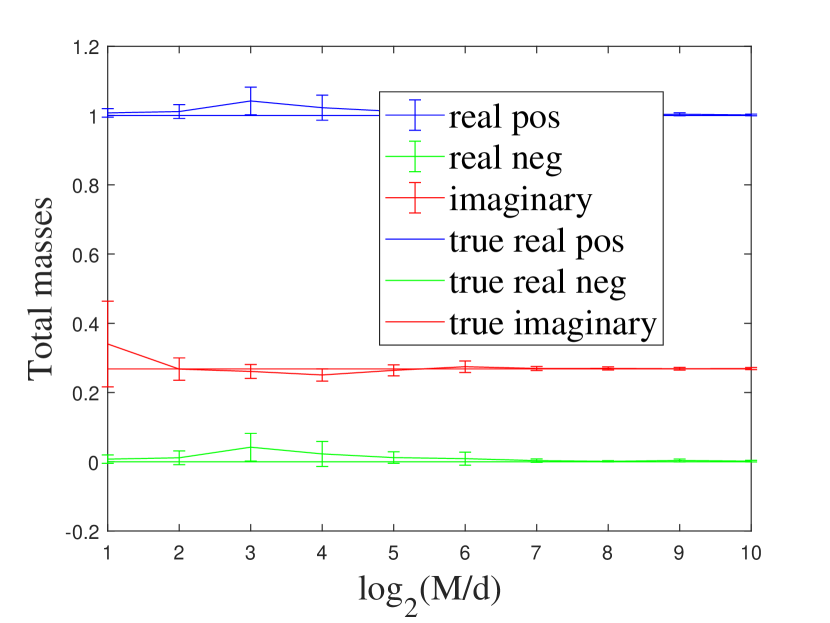
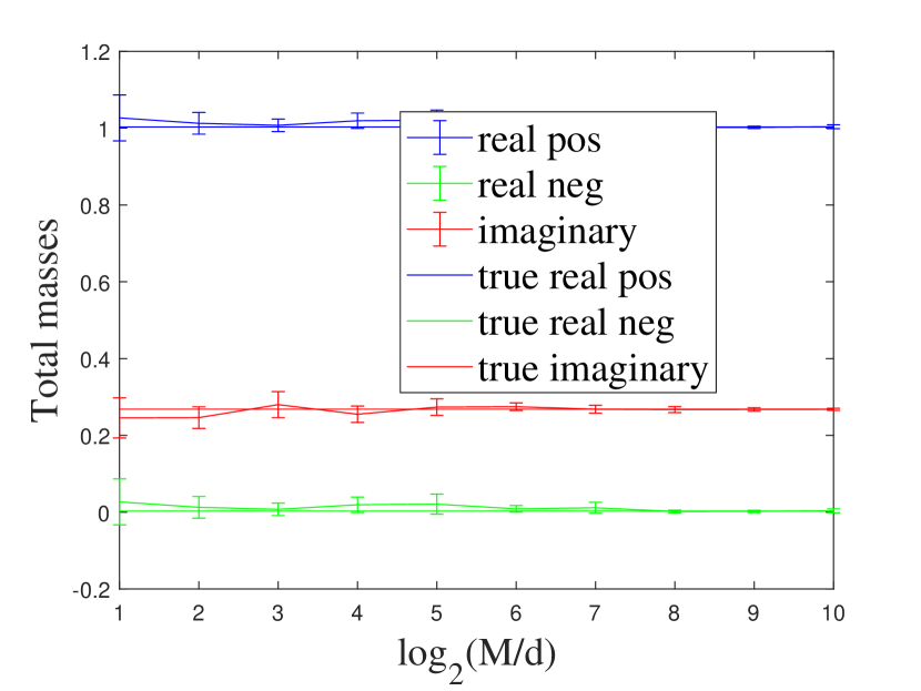
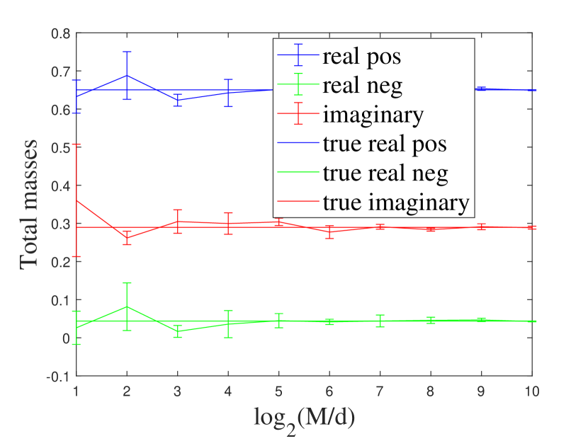
We first estimate the total masses with Ns=10subscript𝑁𝑠10N_{s}=10 on 200020002000 random points sampled from a 111 dimensional Gaussian distribution as a toy example. In this case, the total mass can be accurately calculated and then can be used to evaluate the performance of our estimation. The results is plotted in Figure 1, where the solid lines are the accurate total masses calculated by numerical integral. The bars show the average and standard deviation of estimated total masses. Overall, the estimated total masses stabilize around the accurate total masses and the standard deviation decrease as #random features increases. The proposed optimization provides a valid estimation for total masses even if Nssubscript𝑁𝑠N_{s} is sufficiently small, which illustrates the effectiveness of our estimation method.
Refer to caption
Refer to caption
Refer to caption
Figure 1: Estimated and accurate total masses of three asymmetric kernels (left: Shift-Gaussian; middle: Sinh-Gaussian; right: Cosh-Gaussian) over 1-dimensional data with hyperparameter Ns=10subscript𝑁𝑠10N_{s}=10. “real pos”, “real neg” and “imaginary” on the legend are the estimation bars with the average and the standard deviation, respectively. “true real pos”, “true real neg” and “true imaginary” on the legend are the accurate total masses, respectively. We report the average and the standard deviation of the estimation result (12) over 10 trials, against #random features log2(M/d)subscript2𝑀𝑑\log_{2}(M/d).

5.2 Kernel approximation

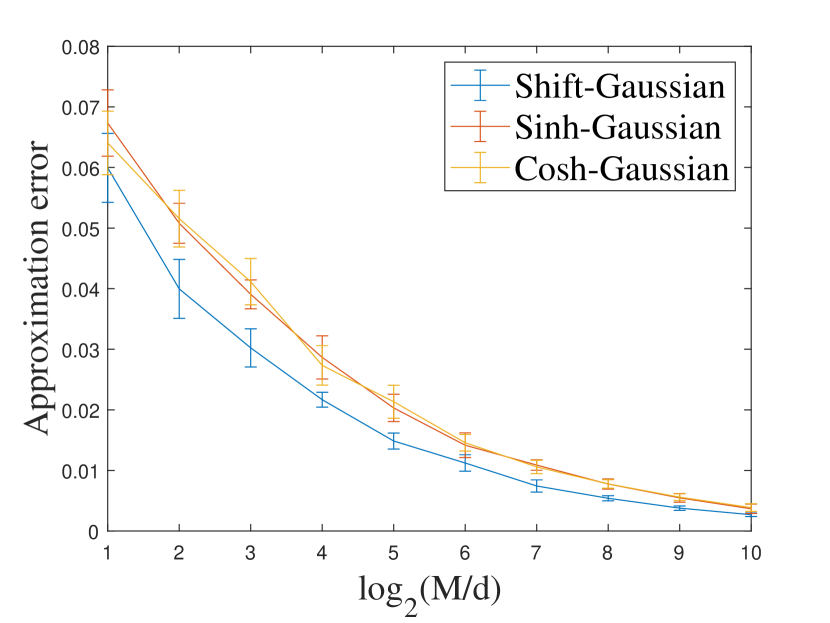
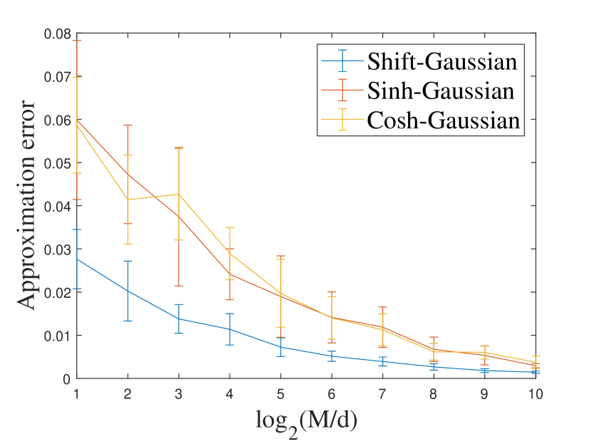
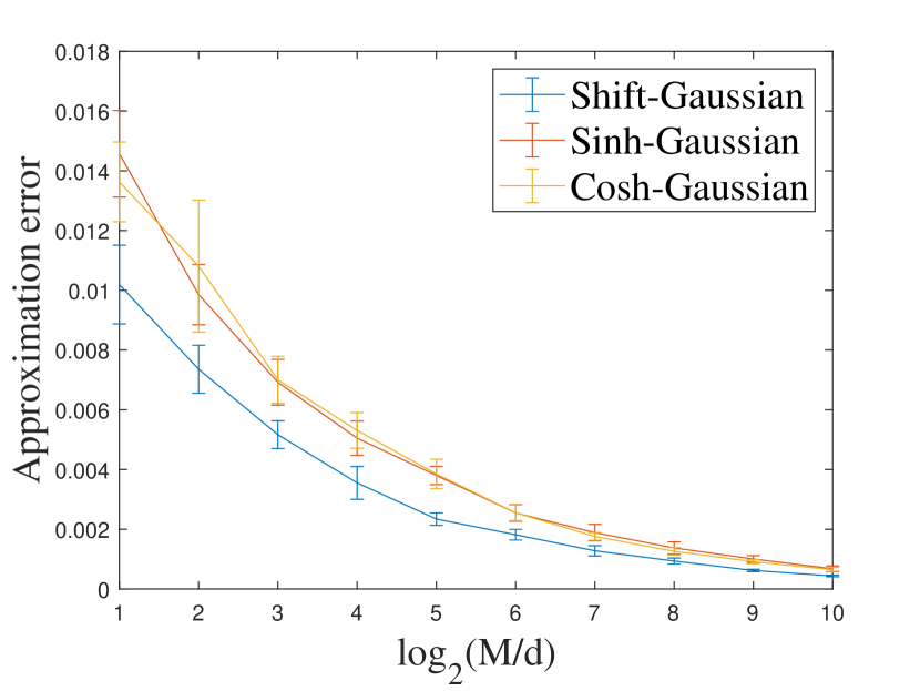
Next, we evaluate the kernel approximation performance of AsK-RFFs. Suppose 𝑲𝑲\bm{K} and 𝑲~~𝑲\widetilde{\bm{K}} are the exact Gram matrix and the approximated Gram matrix on 100010001000 random selected samples, respectively. We use the relative error 𝑲𝑲~F/𝑲Fsubscriptnorm𝑲~𝑲𝐹subscriptnorm𝑲𝐹\|\bm{K}-\widetilde{\bm{K}}\|_{F}/\|\bm{K}\|_{F} to measure the approximation error, where F\|\cdot\|_{F} denotes the Frobenius norm. Figure 2 demonstrate the approximation error bars for three asymmetric kernels in terms of #random features M=d×[21,22,,29,210]𝑀𝑑superscript21superscript22superscript29superscript210M=d\times[2^{1},2^{2},\cdots,2^{9},2^{10}] on four datasets. It is clear that the average approximation error of AsK-RFFs decreases as M𝑀M increases on the four datasets and AsK-RFFs can effectively approximate asymmetric kernel functions. Furthermore, as M𝑀M increases, the approximation performance becomes more stable, i.e., the standard deviations reduce significantly. The experimental results perfectly coincide with Proposition 6.
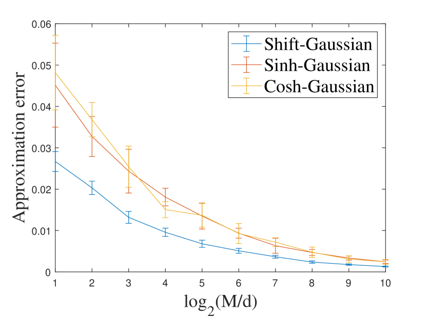
Refer to caption
(a) spambase
Refer to caption
(b) letter
Refer to caption
(c) ijcnn1
Refer to caption
(d) cod-RNA
Figure 2: The approximation error bars across three asymmetric kernels on the four benchmark datasets. For each dataset, we run Algorithm 2 with Ns=50subscript𝑁𝑠50N_{s}=50 over 10 trials and plot the average and the standard deviation of the approximation error against #random features log2(M/d)subscript2𝑀𝑑\log_{2}(M/d).

5.3 Classification

After obtaining the explicit feature mapping, one can apply linear classifiers, e.g., Liblinear (Fan et al.,, 2008), for nonlinear tasks. According to the AsK-RFFs method shown in (7) and (8), we can obtain a pair of features for each asymmetric kernel function. In this paper, we concatenate two random features as an explicit feature mapping Φ(x)=[μR+ϕ(𝝎,𝒙),𝗂μRϕ(𝜻,𝒙),2μI+ϕ(𝝂,𝒙),2μI+ψ(𝝂,𝒙)]Φ𝑥superscriptnormsuperscriptsubscript𝜇𝑅italic-ϕsuperscript𝝎𝒙top𝗂normsuperscriptsubscript𝜇𝑅italic-ϕsuperscript𝜻𝒙top2normsuperscriptsubscript𝜇𝐼italic-ϕsuperscript𝝂𝒙top2normsuperscriptsubscript𝜇𝐼𝜓superscript𝝂𝒙toptop\Phi(x)=\left[\sqrt{\|\mu_{R}^{+}\|}\phi(\bm{\omega},\bm{x})^{\top},\mathsf{i}\sqrt{\|\mu_{R}^{-}\|}\phi(\bm{\zeta},\bm{x})^{\top},\sqrt{2\|\mu_{I}^{+}\|}\phi(\bm{\nu},\bm{x})^{\top},\sqrt{2\|\mu_{I}^{+}\|}\psi(\bm{\nu},\bm{x})^{\top}\right]^{\top} which is then send to LibLinear. The hyperparameter in Liblinear is tuned by 5-folds cross-validation on a parameter grid C=[25,24,,24,25]𝐶superscript25superscript24superscript24superscript25C=\left[2^{-5},2^{-4},\cdots,2^{4},2^{5}\right].

Refer to caption
Refer to caption
Refer to caption
Refer to caption
Refer to caption
Refer to caption
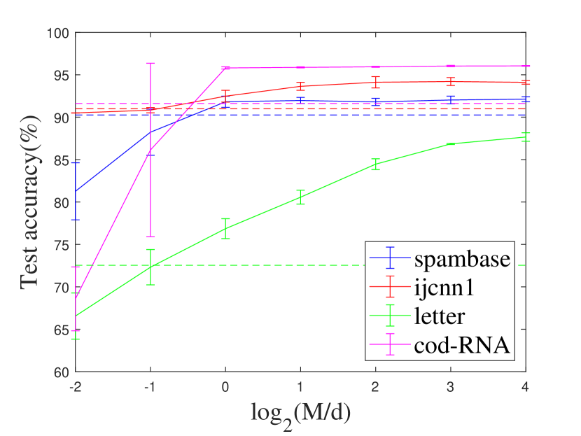
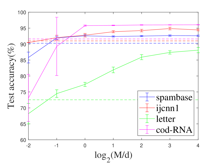
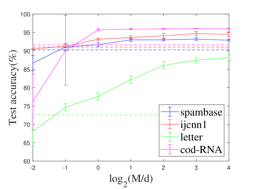
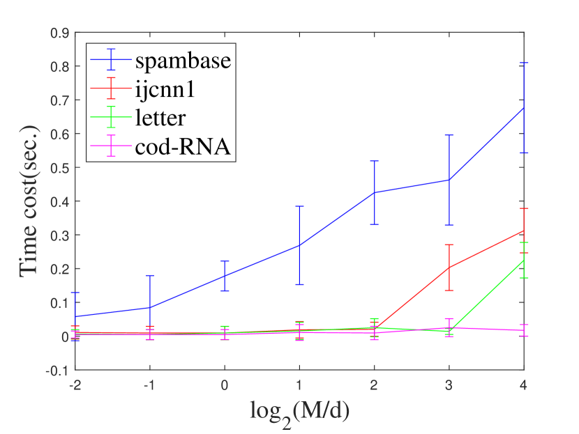
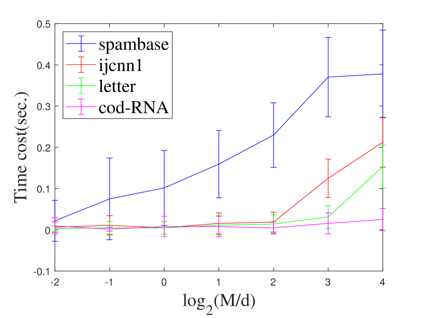
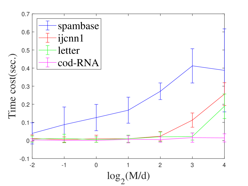
Figure 3: Comparisons of asymmetric kernels for the classification accuracy and sampling time cost with LibLinear on the four datasets. For each asymmetric kernel (left: Shift-Gaussian; middle: Sinh-Gaussian; right: Cosh-Gaussian), we run Algorithm 2 with Ns=50subscript𝑁𝑠50N_{s}=50 over 10 trials and plot the test accuracy bars and sampling time cost bars against #random features log2(M/d)subscript2𝑀𝑑\log_{2}(M/d).

Test accuracy and sampling time cost across three asymmetric kernels on the four datasets are illustrated in Figure 3. The accuracy of a linear classifier is given by dashed lines for reference and the solid bars reflect how well the AsK-RFFs extracts information from nonlinear kernels. It also could be found that with more random features, the accuracy is generally higher until saturation and the AsK-RFFs performs better than the linear classifier when Md𝑀𝑑M\geq d. But with more features, the AsK-RFF needs more computational time, which, however, is always significantly cheaper to calculate the kernel function and solve SVMs in the dual space.

5.4 Asymmetric kernels vs symmetric kernels

The above experiments verified that AsK-RFF can efficiently approximate asymmetric kernels in the view of both kernel approximation and classification. Another possible way of handling asymmetric kernels is to make them symmetric, e.g., K+K2superscript𝐾top𝐾2\frac{K^{\top}+K}{2}, and then extract regular RFFs from the symmetric part. Here in this part, we compare the performance of AsK-RFF and RFF of the above symmetrization method. Additionally, symmetric kernels, including the linear and the radial basis kernel (RBF), are compared as well. Here, the number of random features is M=2d𝑀2𝑑M=2d and the bandwidth of the RBF kernel is 222.

The results are reported in Table 1 where “Asy” and “Sym” denote the asymmetric kernel and its symmetric part, respectively. Generally, Ask-RFFs output a higher classification accuracy than their symmetric parts, the RBF kernel, and the linear kernel. The better performance over RBF, especially there is nearly 5%percent55\% improvement on “letter”, shows that when asymmetric information is crucial, asymmetric kernels may be good choice. The better performance over RFF on the symmetric part, a.k. “Sym”, verifies the effectiveness of AsK-RFF for approximating asymmetric kernels.

Table 1: Test accuracy (the average and the standard deviation over 10 tirals) for different kernels and different approximation methods.
Datasets spambase ijcnn1 letter cod-RNA
Dimension 57 16 22 8
#Train 2760 12000 49990 59535
#Test 1841 6000 91701 271617
Shift- Asy 92.689±plus-or-minus\pm0.207 93.763±plus-or-minus\pm0.599 80.631±plus-or-minus\pm1.269 95.881±plus-or-minus\pm0.122
Gaussian Sym 92.591±plus-or-minus\pm0.228 93.180±plus-or-minus\pm0.614 77.975±plus-or-minus\pm1.229 95.789±plus-or-minus\pm0.008
Sinh- Asy 92.787±plus-or-minus\pm0.351 93.683±plus-or-minus\pm0.481 82.455±plus-or-minus\pm0.851 95.932±plus-or-minus\pm0.001
Gaussian Sym 92.624±plus-or-minus\pm0.247 93.110±plus-or-minus\pm0.587 78.553±plus-or-minus\pm0.806 95.866±plus-or-minus\pm0.011
Cosh- Asy 92.787±plus-or-minus\pm0.210 93.583±plus-or-minus\pm0.278 82.237±plus-or-minus\pm1.206 95.95±plus-or-minus\pm0.038
Gaussian Sym 92.520±plus-or-minus\pm0.210 93.464±plus-or-minus\pm0.406 77.652±plus-or-minus\pm1.585 95.794±plus-or-minus\pm0.008
RBF 92.461±plus-or-minus\pm0.300 93.157±plus-or-minus\pm0.548 77.547±plus-or-minus\pm1.158 95.831±plus-or-minus\pm0.069
Linear 90.261±plus-or-minus\pm0.120 91.011±plus-or-minus\pm0.048 72.541±plus-or-minus\pm0.029 91.618±plus-or-minus\pm0.002

6 Conclusion

In this paper, we investigated a unified kernel approximation framework by RFFs which can uniformly approximate asymmetric kernels. A spectral representation of asymmetric kernels via complex measure was presented by the proposed AsK-RFFs method which could be applied to both asymmetric and symmetric kernels including positive definite and indefinite kernels. In this framework, we could design kernels by altering their complex measures from a statistics perspective. Besides, we proposed a subset-based fast estimation method for total masses on a sub-training set to speed up our approximation process. The effecietnveness of AsK-RFFs was evaluated in experimental results on several large classification datasets. Another intererting avenue for asymmetric kernel approximation is the Nyström-type method (Williams and Seeger,, 2001; Drineas et al.,, 2005). The Nyström-type approximation process that uses low-rank matrices to approximate the asymmetric kernel matrix is worthy of further research.

Appendix A Proof of Proposition 6

The proof strategy closely follows which of (Rahimi and Recht,, 2007; Sutherland and Schneider,, 2015). Suppose k(𝚫)𝑘𝚫k(\bm{\Delta}) is twice differentiable. Denote f(𝚫):=s(𝚫)k(𝚫)assign𝑓𝚫𝑠𝚫𝑘𝚫f(\bm{\Delta}):=s(\bm{\Delta})-k(\bm{\Delta}). Let 𝒳Δ={𝒙𝒚|𝒙,𝒚𝒳}subscript𝒳bold-script-Δconditional-set𝒙𝒚𝒙𝒚𝒳\mathcal{X_{\bm{\Delta}}}=\{\bm{x}-\bm{y}|\bm{x},\bm{y}\in\mathcal{X}\} which is compact with diameter l𝑙l. An ϵitalic-ϵ\epsilon-net can be found that covers 𝒳Δsubscript𝒳bold-script-Δ\mathcal{X_{\bm{\Delta}}} with at most T=(4lr)d𝑇superscript4𝑙𝑟𝑑T=(\frac{4l}{r})^{d} balls of radius r𝑟r (Cucker and Smale,, 2002). Let {𝚫𝒌}k=1Tsuperscriptsubscriptsubscript𝚫𝒌𝑘1𝑇\{\bm{\Delta_{k}}\}_{k=1}^{T} be centers and Lfsubscript𝐿𝑓L_{f} be the Lipschitz constant of f𝑓f. There is a fact that |f(𝚫)|<ϵ𝑓𝚫italic-ϵ|f(\bm{\Delta})|<\epsilon for all 𝚫𝒳Δ𝚫subscript𝒳bold-script-Δ\bm{\Delta}\in\mathcal{X_{\bm{\Delta}}} if |f(𝚫𝒌)|<ϵ2𝑓subscript𝚫𝒌italic-ϵ2|f(\bm{\Delta_{k}})|<\frac{\epsilon}{2} and Lf<ϵ2rsubscript𝐿𝑓italic-ϵ2𝑟L_{f}<\frac{\epsilon}{2r} for all k𝑘k.

Since f𝑓f is differentiable, we denote Lf=f(𝚫)subscript𝐿𝑓𝑓superscript𝚫L_{f}=\triangledown f(\bm{\Delta}^{\star}) where 𝚫=argmax𝚫𝒳Δf(𝚫)superscript𝚫subscript𝚫subscript𝒳bold-script-Δnorm𝑓𝚫\bm{\Delta}^{\star}=\arg\max_{\bm{\Delta}\in\mathcal{X_{\bm{\Delta}}}}\|\triangledown f(\bm{\Delta})\|. We have

𝔼[Lf2]𝔼delimited-[]superscriptsubscript𝐿𝑓2\displaystyle\mathbb{E}[L_{f}^{2}] =𝔼f(𝚫)2absent𝔼superscriptnorm𝑓superscript𝚫2\displaystyle=\mathbb{E}\|\triangledown f(\bm{\Delta}^{\star})\|^{2}
𝔼s(𝚫)2𝔼k(𝚫)2absent𝔼superscriptnorm𝑠superscript𝚫2𝔼superscriptnorm𝑘superscript𝚫2\displaystyle\leq\mathbb{E}\|\triangledown s(\bm{\Delta}^{\star})\|^{2}-\mathbb{E}\|\triangledown k(\bm{\Delta}^{\star})\|^{2}
𝔼s(𝚫)2absent𝔼superscriptnorm𝑠superscript𝚫2\displaystyle\leq\mathbb{E}\|\triangledown s(\bm{\Delta}^{\star})\|^{2}
=𝔼1Ml=1MμR+cos(𝝎l𝚫)μRcos(𝜻l𝚫)2μI+sin(𝝂l𝚫)2absent𝔼norm1𝑀superscriptsubscript𝑙1𝑀superscriptsubscript𝜇𝑅normlimit-fromsuperscriptsubscript𝝎𝑙topsuperscript𝚫superscriptsubscript𝜇𝑅normsuperscriptsubscript𝜻𝑙topsuperscript𝚫2superscriptsubscript𝜇𝐼superscriptnormsuperscriptsubscript𝝂𝑙topsuperscript𝚫2\displaystyle=\mathbb{E}\big{\|}\frac{1}{M}\triangledown\sum_{l=1}^{M}\|\mu_{R}^{+}\|\cos(\bm{\omega}_{l}^{\top}\bm{\Delta}^{\star})-\|\mu_{R}^{-}\|\cos(\bm{\zeta}_{l}^{\top}\bm{\Delta}^{\star})-2\|\mu_{I}^{+}\|\sin(\bm{\nu}_{l}^{\top}\bm{\Delta}^{\star})\big{\|}^{2}
=𝔼[μR+cos(𝝎𝚫)μRcos(𝜻𝚫)2μI+sin(𝝂𝚫)]2absent𝔼superscriptnormdelimited-[]normsuperscriptsubscript𝜇𝑅superscript𝝎topsuperscript𝚫normsuperscriptsubscript𝜇𝑅superscript𝜻topsuperscript𝚫2normsuperscriptsubscript𝜇𝐼superscript𝝂topsuperscript𝚫2\displaystyle=\mathbb{E}\big{\|}\triangledown\big{[}\|\mu_{R}^{+}\|\cos(\bm{\omega}^{\top}\bm{\Delta}^{\star})-\|\mu_{R}^{-}\|\cos(\bm{\zeta}^{\top}\bm{\Delta}^{\star})-2\|\mu_{I}^{+}\|\sin(\bm{\nu}^{\top}\bm{\Delta}^{\star})\big{]}\big{\|}^{2}
=𝔼μR+sin(𝝎𝚫)𝝎μRsin(𝜻𝚫)𝜻+2μI+cos(𝝂𝚫)𝝂2absent𝔼superscriptnormnormsuperscriptsubscript𝜇𝑅superscript𝝎topsuperscript𝚫𝝎normsuperscriptsubscript𝜇𝑅superscript𝜻topsuperscript𝚫𝜻2normsuperscriptsubscript𝜇𝐼superscript𝝂topsuperscript𝚫𝝂2\displaystyle=\mathbb{E}\left\|\|\mu_{R}^{+}\|\sin(\bm{\omega}^{\top}\bm{\Delta}^{\star})\bm{\omega}-\|\mu_{R}^{-}\|\sin(\bm{\zeta}^{\top}\bm{\Delta}^{\star})\bm{\zeta}+2\|\mu_{I}^{+}\|\cos(\bm{\nu}^{\top}\bm{\Delta}^{\star})\bm{\nu}\right\|^{2}
𝔼[|sin(𝝎𝚫)|μR+𝝎+|sin(𝜻𝚫)|μR𝜻\displaystyle\leq\mathbb{E}\big{[}|\sin(\bm{\omega}^{\top}\bm{\Delta}^{\star})|\cdot\|\mu_{R}^{+}\|\|\bm{\omega}\|+|\sin(\bm{\zeta}^{\top}\bm{\Delta}^{\star})|\cdot\|\mu_{R}^{-}\|\|\bm{\zeta}\|
+2|cos(𝝂𝚫)|μI+𝝂]2\displaystyle\quad+2|\cos(\bm{\nu}^{\top}\bm{\Delta}^{\star})|\cdot\|\mu_{I}^{+}\|\|\bm{\nu}\|\big{]}^{2}
𝔼[μR+𝝎+μR𝜻+2μI+𝝂]2absent𝔼superscriptdelimited-[]normsuperscriptsubscript𝜇𝑅norm𝝎normsuperscriptsubscript𝜇𝑅norm𝜻2normsuperscriptsubscript𝜇𝐼norm𝝂2\displaystyle\leq\mathbb{E}\big{[}\|\mu_{R}^{+}\|\cdot\|\bm{\omega}\|+\|\mu_{R}^{-}\|\cdot\|\bm{\zeta}\|+2\|\mu_{I}^{+}\|\cdot\|\bm{\nu}\|\big{]}^{2}
𝔼[(μR+2+μR2+(2μI+)2)(𝝎2+𝜻2+(2𝝂)2)]absent𝔼delimited-[]superscriptnormsuperscriptsubscript𝜇𝑅2superscriptnormsuperscriptsubscript𝜇𝑅2superscript2normsuperscriptsubscript𝜇𝐼2superscriptnorm𝝎2superscriptnorm𝜻2superscript2norm𝝂2\displaystyle\leq\mathbb{E}\left[\left(\|\mu_{R}^{+}\|^{2}+\|\mu_{R}^{-}\|^{2}+(\sqrt{2}\|\mu_{I}^{+}\|)^{2}\right)\cdot\left(\|\bm{\omega}\|^{2}+\|\bm{\zeta}\|^{2}+(\sqrt{2}\|\bm{\nu}\|)^{2}\right)\right]
=(μR+2+μR2+2μI+2)𝔼(𝝎2+𝜻2+2𝝂2):=αμ2.absentsuperscriptnormsuperscriptsubscript𝜇𝑅2superscriptnormsuperscriptsubscript𝜇𝑅22superscriptnormsuperscriptsubscript𝜇𝐼2𝔼superscriptnorm𝝎2superscriptnorm𝜻22superscriptnorm𝝂2assignsuperscriptsubscript𝛼𝜇2\displaystyle=\left(\|\mu_{R}^{+}\|^{2}+\|\mu_{R}^{-}\|^{2}+2\|\mu_{I}^{+}\|^{2}\right)\cdot\mathbb{E}\left(\|\bm{\omega}\|^{2}+\|\bm{\zeta}\|^{2}+2\|\bm{\nu}\|^{2}\right):=\alpha_{\mu}^{2}\,.

The first and second inequalities are derived in a similar fashion with (Sutherland and Schneider,, 2015). The third inequality is from the triangle inequality a+b+ca+b+cnorm𝑎𝑏𝑐norm𝑎norm𝑏norm𝑐\|a+b+c\|\leq\|a\|+\|b\|+\|c\| with a,b,c𝑎𝑏𝑐a,b,c being vectors. The fourth inequality holds because the sine and cosine functions are bounded by ±1plus-or-minus1\pm 1. The fifth inequality is from the Cauchy–Schwarz inequality (i=1nuivi)2(i=1nui2)(i=1nvi2)superscriptsuperscriptsubscript𝑖1𝑛subscript𝑢𝑖subscript𝑣𝑖2superscriptsubscript𝑖1𝑛superscriptsubscript𝑢𝑖2superscriptsubscript𝑖1𝑛superscriptsubscript𝑣𝑖2(\sum_{i=1}^{n}u_{i}v_{i})^{2}\leq(\sum_{i=1}^{n}u_{i}^{2})(\sum_{i=1}^{n}v_{i}^{2}) with ui,visubscript𝑢𝑖subscript𝑣𝑖u_{i},v_{i} being real numbers.

According to the Markov’s inequality, we obtain a probability bound for the Lipschitz constant,

Pr(Lfϵ2r)=Pr(Lf2(ϵ2r)2)αμ2(2rϵ)2.Prsubscript𝐿𝑓italic-ϵ2𝑟Prsuperscriptsubscript𝐿𝑓2superscriptitalic-ϵ2𝑟2superscriptsubscript𝛼𝜇2superscript2𝑟italic-ϵ2{\rm Pr}\left(L_{f}\geq\frac{\epsilon}{2r}\right)={\rm Pr}\left(L_{f}^{2}\geq(\frac{\epsilon}{2r})^{2}\right)\leq\alpha_{\mu}^{2}\left(\frac{2r}{\epsilon}\right)^{2}\,. (13)

Given a fixed 𝚫𝚫\bm{\Delta}, s(𝚫)𝑠𝚫s(\bm{\Delta}) is bounded by ±(μR++μR+2μI+)plus-or-minusnormsuperscriptsubscript𝜇𝑅normsuperscriptsubscript𝜇𝑅2normsuperscriptsubscript𝜇𝐼\pm\left(\|\mu_{R}^{+}\|+\|\mu_{R}^{-}\|+2\|\mu_{I}^{+}\|\right) with the expectation k(𝚫)𝑘𝚫k(\bm{\Delta}). Applying the Hoeffding’s inequality and a union bound to anchors in the ϵitalic-ϵ\epsilon-net, we have

Pr(k=1T|f(𝚫𝒌)|ϵ2)TPr(|f(𝚫𝒌)|ϵ2)2Texp(Mϵ28μ2).Prsuperscriptsubscript𝑘1𝑇𝑓subscript𝚫𝒌italic-ϵ2𝑇Pr𝑓subscript𝚫𝒌italic-ϵ22𝑇𝑀superscriptitalic-ϵ28superscriptnorm𝜇2{\rm Pr}\left(\cup_{k=1}^{T}|f(\bm{\Delta_{k}})|\geq\frac{\epsilon}{2}\right)\leq T{\rm Pr}\left(|f(\bm{\Delta_{k}}\right)|\geq\frac{\epsilon}{2})\leq 2T\exp\left(-\frac{M\epsilon^{2}}{8\|\mu\|^{2}}\right)\,. (14)

Combining bounds (13) and (14), we obtain a bound in terms of r𝑟r,

Pr(sup𝚫𝒳Δ|f(𝚫)|ϵ)1κ1rdκ2r2,Prsubscriptsupremum𝚫subscript𝒳bold-script-Δ𝑓𝚫italic-ϵ1subscript𝜅1superscript𝑟𝑑subscript𝜅2superscript𝑟2{\rm Pr}\left(\sup_{\bm{\Delta}\in\mathcal{X_{\bm{\Delta}}}}|f(\bm{\Delta})|\leq\epsilon\right)\geq 1-\kappa_{1}r^{-d}-\kappa_{2}r^{2},

where κ1=2(4l)dexp(Mϵ28μ2)subscript𝜅12superscript4𝑙𝑑𝑀superscriptitalic-ϵ28superscriptnorm𝜇2\kappa_{1}=2(4l)^{d}\exp\left(-\frac{M\epsilon^{2}}{8\|\mu\|^{2}}\right) , κ2=4αμ2ϵ2subscript𝜅24superscriptsubscript𝛼𝜇2superscriptitalic-ϵ2\kappa_{2}=4\alpha_{\mu}^{2}\epsilon^{-2}. We choose r𝑟r such that dκ1rd12κ2r=0𝑑subscript𝜅1superscript𝑟𝑑12subscript𝜅2𝑟0d\kappa_{1}r^{-d-1}-2\kappa_{2}r=0 i.e., r=(dκ12κ2)1d+2𝑟superscript𝑑subscript𝜅12subscript𝜅21𝑑2r=\left(\frac{d\kappa_{1}}{2\kappa_{2}}\right)^{\frac{1}{d+2}}, as did in (Sutherland and Schneider,, 2015). Then we have a bound

Pr(sup𝚫𝒳Δ|f(𝚫)|>ϵ)Prsubscriptsupremum𝚫subscript𝒳bold-script-Δ𝑓𝚫italic-ϵ\displaystyle{}{\rm Pr}\left(\sup_{\bm{\Delta}\in\mathcal{X_{\bm{\Delta}}}}|f(\bm{\Delta})|>\epsilon\right) ((d2)dd+2+(d2)2d+2)26d+2d+2(αμlϵ)2dd+2exp(Mϵ24(d+2)μ2)absentsuperscript𝑑2𝑑𝑑2superscript𝑑22𝑑2superscript26𝑑2𝑑2superscriptsubscript𝛼𝜇𝑙italic-ϵ2𝑑𝑑2𝑀superscriptitalic-ϵ24𝑑2superscriptnorm𝜇2\displaystyle\leq\left((\frac{d}{2})^{\frac{-d}{d+2}}+(\frac{d}{2})^{\frac{2}{d+2}}\right)\cdot 2^{\frac{6d+2}{d+2}}\left(\frac{\alpha_{\mu}l}{\epsilon}\right)^{\frac{2d}{d+2}}\exp\left(\frac{-M\epsilon^{2}}{4(d+2)\|\mu\|^{2}}\right)
=βd(αμlϵ)2dd+2exp(ϵ2M4(d+2)μ2).absentsubscript𝛽𝑑superscriptsubscript𝛼𝜇𝑙italic-ϵ2𝑑𝑑2superscriptitalic-ϵ2𝑀4𝑑2superscriptnorm𝜇2\displaystyle=\beta_{d}\left(\frac{\alpha_{\mu}l}{\epsilon}\right)^{\frac{2d}{d+2}}\exp\left(\frac{-\epsilon^{2}M}{4(d+2)\|\mu\|^{2}}\right)\,.

Thus, we can control the pointwise error no more than ϵitalic-ϵ\epsilon with probability at least 1δ1𝛿1-\delta as long as M4(d+2)μ2ϵ2(logβdδ+2dd+2logαμlϵ)𝑀4𝑑2superscriptnorm𝜇2superscriptitalic-ϵ2subscript𝛽𝑑𝛿2𝑑𝑑2subscript𝛼𝜇𝑙italic-ϵM\geq 4(d+2)\|\mu\|^{2}\epsilon^{-2}\left(\log\frac{\beta_{d}}{\delta}+\frac{2d}{d+2}\log\frac{\alpha_{\mu}l}{\epsilon}\right). Sutherland and Schneider, (2015) provide the maximum value β64=66subscript𝛽6466\beta_{64}=66 and asymptotic values limdβd=64subscript𝑑subscript𝛽𝑑64\lim_{d\rightarrow\infty}\beta_{d}=64 and the exponent of the second factor can be loosened to 2 if αμlϵsubscript𝛼𝜇𝑙italic-ϵ\alpha_{\mu}l\geq\epsilon.

Appendix B Proof of the Acceptance-Rejection sampling algorithm works

Denote F(𝒕):=f(𝜻𝒕)assign𝐹𝒕𝑓𝜻𝒕F(\bm{t}):=f(\bm{\zeta}\leq\bm{t}) and G(𝒕):=g(𝜻𝒕)assign𝐺𝒕𝑔𝜻𝒕G(\bm{t}):=g(\bm{\zeta}\leq\bm{t}). Denote two events A={𝜻𝒕}𝐴𝜻𝒕A=\{\bm{\zeta}\leq\bm{t}\} and B={Uf(𝜻)cg(𝜻)}𝐵𝑈𝑓𝜻𝑐𝑔𝜻B=\{U\leq\frac{f(\bm{\zeta})}{cg(\bm{\zeta})}\}. Then, F/f𝐹norm𝑓F/\|f\| and G/g𝐺norm𝑔G/\|g\| are two probability measures. Suppose a r.v. 𝜻𝜻\bm{\zeta} is sampled from a distribution G/g𝐺norm𝑔G/\|g\| and a r.v. U𝑈U is sampled from a uniform distribution 𝒰[0,1]𝒰01\mathcal{U}[0,1].

We need to prove Pr(A|B)=F/fPrconditional𝐴𝐵𝐹norm𝑓{\rm Pr}(A|B)=F/\|f\|. To this end, we utilize the Bayes’ theorem, i.e., Pr(A|B)=Pr(B|A)Pr(A)/Pr(B)Prconditional𝐴𝐵Prconditional𝐵𝐴Pr𝐴Pr𝐵{\rm Pr}(A|B)={\rm Pr}(B|A)\cdot{\rm Pr}(A)/{\rm Pr}(B).

Firstly, 𝜻𝜻\bm{\zeta} follows the distribution G/g𝐺norm𝑔G/\|g\|, then Pr(A)=Pr(𝜻𝒕)=G(𝒕)/gPr𝐴Pr𝜻𝒕𝐺𝒕norm𝑔{\rm Pr}(A)={\rm Pr}(\bm{\zeta}\leq\bm{t})=G(\bm{t})/\|g\|. Secondly, the probability Pr(B)Pr𝐵{\rm Pr}(B) is given as follows,

Pr(B)Pr𝐵\displaystyle{\rm Pr}(B) =dPr(Uf(𝜻)cg(𝜻)|𝜻=𝒕))Pr(𝜻=𝒕)d𝒕\displaystyle=\int_{\mathbb{R}^{d}}{\rm Pr}\left(U\leq\frac{f(\bm{\zeta})}{cg(\bm{\zeta})}|\bm{\zeta}=\bm{t})\right)\cdot{\rm Pr}(\bm{\zeta}=\bm{t})\mathrm{d}\bm{t}
=df(𝒕)cg(𝒕)g(𝒕)gd𝒕absentsubscriptsuperscript𝑑𝑓𝒕𝑐𝑔𝒕𝑔𝒕norm𝑔differential-d𝒕\displaystyle=\int_{\mathbb{R}^{d}}\frac{f(\bm{t})}{cg(\bm{t})}\cdot\frac{g(\bm{t})}{\|g\|}\mathrm{d}\bm{t}
=fcg.absentnorm𝑓𝑐norm𝑔\displaystyle=\frac{\|f\|}{c\|g\|}.\,

Thirdly, the probability Pr(B|A)Prconditional𝐵𝐴{\rm Pr}(B|A) can be derived by,

Pr(B|A)Prconditional𝐵𝐴\displaystyle{\rm Pr}(B|A) =Pr(Uf(𝜻)cg(𝜻)|𝜻𝒕)absentPr𝑈conditional𝑓𝜻𝑐𝑔𝜻𝜻𝒕\displaystyle={\rm Pr}\left(U\leq\frac{f(\bm{\zeta})}{cg(\bm{\zeta})}|\bm{\zeta}\leq\bm{t}\right)
=Pr(Uf(𝜻)cg(𝜻),𝜻𝒕)Pr(𝜻𝒕)absentPrformulae-sequence𝑈𝑓𝜻𝑐𝑔𝜻𝜻𝒕Pr𝜻𝒕\displaystyle=\frac{{\rm Pr}\left(U\leq\frac{f(\bm{\zeta})}{cg(\bm{\zeta})},\bm{\zeta}\leq\bm{t}\right)}{{\rm Pr}(\bm{\zeta}\leq\bm{t})}
=gG(𝒕)[]d𝒕Pr(Uf(𝜻)cg(𝜻)|𝜻=𝒘𝒕)g(𝒘)gd𝒘absentnorm𝑔𝐺𝒕superscriptsubscriptsuperscriptdelimited-[]𝑑𝒕Pr𝑈conditional𝑓𝜻𝑐𝑔𝜻𝜻𝒘𝒕𝑔𝒘norm𝑔differential-d𝒘\displaystyle=\frac{\|g\|}{G(\bm{t})}\int_{[-\infty]^{d}}^{\bm{t}}{\rm Pr}\left(U\leq\frac{f(\bm{\zeta})}{cg(\bm{\zeta})}|\bm{\zeta}=\bm{w}\leq\bm{t}\right)\cdot\frac{g(\bm{w})}{\|g\|}\mathrm{d}\bm{w}
=gG(𝒕)[]d𝒕f(𝒘)cg(𝒘)g(𝒘)gd𝒘absentnorm𝑔𝐺𝒕superscriptsubscriptsuperscriptdelimited-[]𝑑𝒕𝑓𝒘𝑐𝑔𝒘𝑔𝒘norm𝑔differential-d𝒘\displaystyle=\frac{\|g\|}{G(\bm{t})}\int_{[-\infty]^{d}}^{\bm{t}}\frac{f(\bm{w})}{cg(\bm{w})}\frac{g(\bm{w})}{\|g\|}\mathrm{d}\bm{w}
=F(t)cG(t).absent𝐹𝑡𝑐𝐺𝑡\displaystyle=\frac{F(t)}{cG(t)}.\,

Then, the probability Pr(𝜻𝒕|Uf(𝜻)cg(𝜻))=Pr(A|B)Pr𝜻conditional𝒕𝑈𝑓𝜻𝑐𝑔𝜻Prconditional𝐴𝐵{\rm Pr}\left(\bm{\zeta}\leq\bm{t}|U\leq\frac{f(\bm{\zeta})}{cg(\bm{\zeta})}\right)={\rm Pr}(A|B) can be calculated by the following equation.

Pr(𝜻𝒕|Uf(𝜻)cg(𝜻))Pr𝜻conditional𝒕𝑈𝑓𝜻𝑐𝑔𝜻\displaystyle{\rm Pr}\left(\bm{\zeta}\leq\bm{t}|U\leq\frac{f(\bm{\zeta})}{cg(\bm{\zeta})}\right) =Pr(A|B)absentPrconditional𝐴𝐵\displaystyle={\rm Pr}(A|B)
=Pr(B|A)Pr(A)Pr(B)absentPrconditional𝐵𝐴Pr𝐴Pr𝐵\displaystyle=\frac{{\rm Pr}(B|A)\cdot{\rm Pr}(A)}{{\rm Pr}(B)}
=F(t)cG(t)G(𝒕)gcgfabsent𝐹𝑡𝑐𝐺𝑡𝐺𝒕norm𝑔𝑐norm𝑔norm𝑓\displaystyle=\frac{F(t)}{cG(t)}\cdot\frac{G(\bm{t})}{\|g\|}\cdot\frac{c\|g\|}{\|f\|}
=F(t)f,absent𝐹𝑡norm𝑓\displaystyle=\frac{F(t)}{\|f\|}\,,

which concludes the proof.

Declarations

  • Funding This work was supported by National Natural Science Foundation of China (No. 61977046), Shanghai Municipal Science and Technology Major Project (2021SHZDZX0102).

  • Competing interests The authors declare that they have no known competing financial interests or personal relationships that could have appeared to influence the work reported in this paper.

  • Ethics approval Not applicable.

  • Consent to participate Not applicable.

  • Consent for publication Not applicable.

  • Availability of data and materials Not applicable.

  • Code availability Not applicable.

  • Authors’ contributions Not applicable.

References

  • Athreya and Lahiri, (2006) Athreya, K. B. and Lahiri, S. N. (2006). Measure theory and probability theory, volume 19. Springer.
  • Bartolucci et al., (2021) Bartolucci, F., De Vito, E., Rosasco, L., and Vigogna, S. (2021). Understanding neural networks with reproducing kernel banach spaces. arXiv preprint arXiv:2109.09710.
  • Belkin et al., (2019) Belkin, M., Hsu, D., Ma, S., and Mandal, S. (2019). Reconciling modern machine-learning practice and the classical bias–variance trade-off. Proceedings of the National Academy of Sciences, 116(32):15849–15854.
  • Bochner, (2005) Bochner, S. (2005). Harmonic analysis and the theory of probability. Courier Corporation.
  • Chang and Lin, (2011) Chang, C.-C. and Lin, C.-J. (2011). Libsvm: a library for support vector machines. ACM transactions on intelligent systems and technology (TIST), 2(3):1–27.
  • Cohn, (2013) Cohn, D. L. (2013). Measure theory, volume 1. Springer.
  • Cucker and Smale, (2002) Cucker, F. and Smale, S. (2002). On the mathematical foundations of learning. Bulletin of the American Mathematical Society, 39(1):1–49.
  • Drineas et al., (2005) Drineas, P., Mahoney, M. W., and Cristianini, N. (2005). On the Nyström method for approximating a gram matrix for improved kernel-based learning. Journal of Machine Learning Research, 6:2153–2175.
  • Drucker et al., (1997) Drucker, H., Burges, C. J., Kaufman, L., Smola, A., Vapnik, V., et al. (1997). Support vector regression machines. Advances in Neural Information Processing Systems, 9:155–161.
  • Dua and Graff, (2017) Dua, D. and Graff, C. (2017). UCI machine learning repository.
  • Fan et al., (2008) Fan, R.-E., Chang, K.-W., Hsieh, C.-J., Wang, X.-R., and Lin, C.-J. (2008). Liblinear: A library for large linear classification. Journal of Machine Learning Research, 9:1871–1874.
  • Fasshauer et al., (2015) Fasshauer, G. E., Hickernell, F. J., and Ye, Q. (2015). Solving support vector machines in reproducing kernel banach spaces with positive definite functions. Applied and Computational Harmonic Analysis, 38(1):115–139.
  • Girolami, (2002) Girolami, M. (2002). Mercer kernel-based clustering in feature space. IEEE Transactions on Neural Networks, 13(3):780–784.
  • Hinton and Roweis, (2002) Hinton, G. and Roweis, S. T. (2002). Stochastic neighbor embedding. In Advances in Neural Information Processing Systems, volume 15, pages 833–840. Citeseer.
  • Huang et al., (2021) Huang, B., Li, X., Song, Z., and Yang, X. (2021). FL-NTK: A neural tangent kernel-based framework for federated learning analysis. In International Conference on Machine Learning, pages 4423–4434. PMLR.
  • Huang et al., (2017) Huang, X., Maier, A., Hornegger, J., and Suykens, J. A. K. (2017). Indefinite kernels in least squares support vector machines and principal component analysis. Applied and Computational Harmonic Analysis, 43(1):162–172.
  • Lin et al., (2022) Lin, R. R., Zhang, H. Z., and Zhang, J. (2022). On reproducing kernel banach spaces: Generic definitions and unified framework of constructions. Acta Mathematica Sinica, English Series, pages 1–25.
  • (18) Liu, F., Huang, X., Chen, Y., and Suykens, J. A. K. (2021a). Fast learning in reproducing kernel krein spaces via signed measures. In International Conference on Artificial Intelligence and Statistics, pages 388–396. PMLR.
  • (19) Liu, F., Huang, X., Chen, Y., and Suykens, J. A. K. (2021b). Random features for kernel approximation: A survey on algorithms, theory, and beyond. IEEE Transactions on Pattern Analysis and Machine Intelligence, pages 1–1. doi:https://doi.org/10.1109/TPAMI.2021.3097011.
  • Malach et al., (2020) Malach, E., Yehudai, G., Shalev-Schwartz, S., and Shamir, O. (2020). Proving the lottery ticket hypothesis: Pruning is all you need. In International Conference on Machine Learning, pages 6682–6691. PMLR.
  • Mehrkanoon and Suykens, (2018) Mehrkanoon, S. and Suykens, J. A. K. (2018). Deep hybrid neural-kernel networks using random fourier features. Neurocomputing, 298:46–54.
  • Pennington et al., (2015) Pennington, J., Yu, F. X., and Kumar, S. (2015). Spherical random features for polynomial kernels. In Proceedings of the 28th International Conference on Neural Information Processing Systems-Volume 2, pages 1846–1854.
  • Pinsky, (2008) Pinsky, M. A. (2008). Introduction to Fourier analysis and wavelets, volume 102. American Mathematical Soc.
  • Rahimi and Recht, (2007) Rahimi, A. and Recht, B. (2007). Random features for large-scale kernel machines. In Proceedings of the 20th International Conference on Neural Information Processing Systems, pages 1177–1184.
  • Rahimi and Recht, (2008) Rahimi, A. and Recht, B. (2008). Weighted sums of random kitchen sinks: replacing minimization with randomization in learning. In Proceedings of the 21st International Conference on Neural Information Processing Systems, pages 1313–1320.
  • Schölkopf et al., (1997) Schölkopf, B., Smola, A., and Müller, K.-R. (1997). Kernel principal component analysis. In International Conference on Artificial Neural Networks, pages 583–588. Springer.
  • Schölkopf and Smola, (2002) Schölkopf, B. and Smola, A. J. (2002). Learning with Kernels: Support Vector Machines, Regularization, Optimization, and Beyond. MIT press.
  • Soman et al., (2009) Soman, K., Loganathan, R., and Ajay, V. (2009). Machine Learning with SVM and other Kernel Methods. PHI Learning Pvt. Ltd.
  • Song et al., (2013) Song, G., Zhang, H., and Hickernell, F. J. (2013). Reproducing kernel banach spaces with the \ell1 norm. Applied and Computational Harmonic Analysis, 34(1):96–116.
  • Sutherland and Schneider, (2015) Sutherland, D. J. and Schneider, J. (2015). On the error of random fourier features. In Proceedings of the Thirty-First Conference on Uncertainty in Artificial Intelligence, page 862–871. AUAI Press.
  • Suykens, (2016) Suykens, J. A. K. (2016). SVD revisited: A new variational principle, compatible feature maps and nonlinear extensions. Applied and Computational Harmonic Analysis, 40(3):600–609.
  • Suykens et al., (2002) Suykens, J. A. K., Van Gestel, T., De Brabanter, J., De Moor, B., and Vandewalle, J. (2002). Least Squares Support Vector Machines. World Scientific.
  • (33) Tang, J., Qu, M., and Mei, Q. (2015a). Pte: Predictive text embedding through large-scale heterogeneous text networks. In Proceedings of the 21th ACM SIGKDD International Conference on Knowledge Discovery and Data Mining, pages 1165–1174.
  • (34) Tang, J., Qu, M., Wang, M., Zhang, M., Yan, J., and Mei, Q. (2015b). Line: Large-scale information network embedding. In Proceedings of the 24th International Conference on World Wide Web, pages 1067–1077.
  • Vapnik, (2013) Vapnik, V. (2013). The Nature of Statistical Learning Theory. Springer Science & Business Media.
  • Vaswani et al., (2017) Vaswani, A., Shazeer, N., Parmar, N., Uszkoreit, J., Jones, L., Gomez, A. N., Kaiser, L., and Polosukhin, I. (2017). Attention is all you need. In Proceedings of the 31st International Conference on Neural Information Processing Systems, page 6000–6010. Curran Associates Inc.
  • Suykens, (2017) Suykens, J. A. K. (2017). Deep restricted kernel machines using conjugate feature duality. Neural Computation, 29(8):2123–2163.
  • Williams and Seeger, (2001) Williams, C. and Seeger, M. (2001). Using the Nyström method to speed up kernel machines. In Advances in Neural Information Processing Systems 13, pages 682–688. MIT Press.
  • Wright and Gonzalez, (2021) Wright, M. A. and Gonzalez, J. E. (2021). Transformers are deep infinite-dimensional non-mercer binary kernel machines. arXiv preprint arXiv:2106.01506.
  • Zhang et al., (2009) Zhang, H., Xu, Y., and Zhang, J. (2009). Reproducing kernel banach spaces for machine learning. Journal of Machine Learning Research, 10:2741–2775.