Optimal empirical Bayes estimation for the Poisson model via minimum-distance methods

Abstract

The Robbins estimator is the most iconic and widely used procedure in the empirical Bayes literature for the Poisson model. On one hand, this method has been recently shown to be minimax optimal in terms of the regret (excess risk over the Bayesian oracle that knows the true prior) for various nonparametric classes of priors. On the other hand, it has been long recognized in practice that Robbins estimator lacks the desired smoothness and monotonicity of Bayes estimators and can be easily derailed by those data points that were rarely observed before. Based on the minimum-distance distance method, we propose a suite of empirical Bayes estimators, including the classical nonparametric maximum likelihood, that outperform the Robbins method in a variety of synthetic and real data sets and retain its optimality in terms of minimax regret.

1 Introduction

Suppose we have an observation $Y$ distributed as $\mathrm{Poi}(\theta)$, the Poisson distribution with an unknown mean $\theta$. In a Bayesian setting, $\theta$ is assumed to sampled from some prior $G$ on the positive real line $\mathbb{R}_{+}$, and the Bayes estimator of $\theta$ minimizing the average loss is the posterior mean $\mathbb{E}\left[\theta|Y\right]$. Denote by $f_{G}$ the marginal distribution of $Y$, given by the mixture of the Poisson mass function $f_{\theta}(y)=e^{-\theta}{\theta^{y}\over y!},y\in\mathbb{Z}_{+}\triangleq\left\{0,1,\dots\right\}$ and the prior distribution $G$:

$$f_{G}(y)=\int f_{\theta}(y)G(d\theta)$$ (1)

Then the Bayes estimator of $\theta$ is given by

$$\widehat{\theta}_{G}(Y)=\mathbb{E}_{G}\left[\theta|Y\right]={\int\theta e^{-\theta}{\theta^{Y}\over Y!}G(d\theta)\over\int e^{-\theta}{\theta^{Y}\over Y!}G(d\theta)}=(Y+1){f_{G}(Y+1)\over f_{G}(Y)}.$$ (2)

In practice, the prior is rarely known exactly. The main observation of the Empirical Bayes (EB) theory, introduced by Robbins [Rob51, Rob56], is that when independent and seemingly unrelated training samples $Y^{n}\triangleq(Y_{1},\ldots,Y_{n}){\stackrel{{\scriptstyle\text{i.i.d.}}}{{\sim}}}f_{G}$ are available, it is possible to produce approximation of $\widehat{\theta}_{G}(Y)$ that has vanishing regret (excess risk) over the Bayesian oracle that knows the true prior. Since then, the theory and methodology of empirical Bayes have been well developed and widely applied in large-scale data analysis in practice cf. e.g. [ETST01, VH96, Bro08, PLLB10]. We refer the reader to the surveys and monographs on the theory and practice of empirical Bayes [Mor83, Cas85, Zha03, Efr14, ML18, Efr21].

In the literature, there are two main avenues to obtain solutions to the EB problem:

• $f$-modeling: Construct an approximate Bayes estimator by approximating the marginal density. For example, the Robbins estimator [Rob56] is a plug-in estimate of (2) replacing the true $f_{G}$ with the empirical distribution, leading to

  $$\widehat{\theta}_{\text{Robbins}}(Y)\triangleq\widehat{\theta}_{\text{Robbins}}(Y;Y_{1},\dots,Y_{n})=(Y+1){N_{n}(Y+1)\over N_{n}(Y)+1},$$ (3)

  where $N_{n}(y)\triangleq\sum_{i=1}^{n}{{\mathbf{1}_{\left\{{Y_{i}=y}\right\}}}}$ is the empirical count of $y\in\mathbb{Z}_{+}$.

• $g$-modeling: We first obtain an estimate ${\widehat{G}}$ of the prior $G$ from $Y^{n}$ and then apply the corresponding Bayes estimator $\widehat{\theta}_{{\widehat{G}}}(Y)$. Examples of ${\widehat{G}}$ include the celebrated nonparametric maximum likelihood estimator (NPMLE) [KW56]

  $${\widehat{G}}=\mathop{\rm argmax}_{G}\frac{1}{n}\sum_{i=1}^{n}\log f_{G}(Y_{i})$$ (4)

  where the maximization is over all priors on $\mathbb{R}_{+}$ (unconstrained NPMLE). When additional information about the prior is available (e.g., compactly supported), it is convenient to incorporate this as constraints into the above optimization, leading to constrained NPMLE.

In a nutshell, both $f$-modeling and $g$-modeling rely on estimate of the population density $f_{G}$; the difference is that the former applies improper density estimate such as the empirical distribution or kernel density estimate (see, e.g., [LGL05, BG09, Zha09] for Gaussian models), while the latter applies proper density estimate of the form $f_{\widehat{G}}$.

In recent years, there have been significant advances in the theoretical analysis of $f$-modeling EB estimators for the Poisson model, specifically, the Robbins method. For compactly supported priors, [BGR13] showed that with Poisson sampling (replacing the sample size $n$ by $\mathrm{Poi}(n)$), the Robbins estimator achieves a $O\left({(\log n)^{2}\over n(\log\log n)^{2}}\right)$ regret. Later [PW21] showed the same regret bound holds with fixed sample size $n$ and established the optimality of the Robbins estimator by proving a matching minimax lower bound. In addition, for the class of subexponential priors, the Robbins estimator also achieves optimal minimax regret $\Theta\left({(\log n)^{3}\over n}\right)$.

On the other hand, despite its simplicity and optimality, it has been long recognized that the Robbins method often produces unstable estimates in practice. This occurs particularly for those $y$ which appears few times or none whatsoever, so that $N(y)$ is small or zero. Thus, unless $N(y+1)$ is also small, the formula (3) produces exceptionally large value of $\widehat{\theta}_{\text{Robbins}}(y)$. In addition, if $N(y+1)=0$ (e.g., when $y\geq\max\{Y_{1},\ldots,Y_{n}\}$), we have $\widehat{\theta}_{\text{Robbins}}(y)=0$ irrespective of any existing information about $y$, which is at odds with the fact that the Bayes estimator $\widehat{\theta}_{G}(y)$ is always monotonically increasing in $y$ for any $G$ [HS83]. These issues of the Robbins estimator have been well-documented and discussed in the literature; see, for example, [Mar68, Section 1] and [ML18, Section 1.9] for a finite-sample study and [EH21, Section 6.1] for the destabilized behavior of Robbins estimator in practice (e.g., in analyzing insurance claims data). To alleviate the shortcomings of the Robbins estimator, a number of modifications have been proposed [Mar68, BGR13] that enforce smoothness or monotonicity; nevertheless, it is unclear they still retain the regret optimality of the Robbins method. This raises the question of whether it is possible to construct a well-behaved EB estimator that is provably optimal in terms of regret.

In this paper, we answer this question in the positive. This is accomplished by a class of $g$-modeling EB estimators, which are free from the unstable behavior of Robbins estimator, thanks to their Bayesian form which guarantees monotonicity among many other desirable properties. The prior is learned using the minimum-distance method, including the NPMLE (4) as a special case. Introduced in the pioneering works [Wol53, Wol54, Wol57], the minimum-distance method aims to find the best fit in class to the data with respect to a given distance. As such, it is well-suited for the task of estimating the prior and the obtained density estimate is proper and of the desired mixture type.

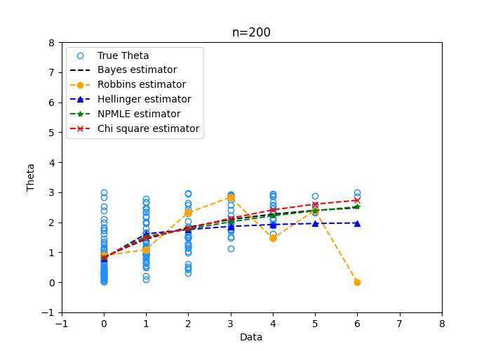
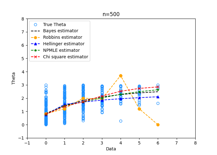
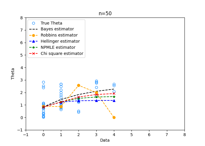
As a concrete example, we consider a simple uniform prior and compare the numerical performance of Robbins and three prototypical examples of minimum-distance estimators of $G$, with respect to the Kullback-Leibler (KL) divergence (i.e., the NPMLE), the Hellinger distance, and the $\chi^{2}$-divergence, respectively (see Section 2.1 for the formal definitions). As evident in Fig. 1, the minimum-distance EB estimators provide a much more consistent approximation of the Bayes estimator compared to the Robbins estimator. This advantage is even more pronounced for unbounded priors (cf. Fig. 4 in Section 5.3); see also Fig. 2 for a real-world example where EB methodology is applied to a prediction task with sports data.

Figure 1: Comparison of Robbins estimator with different minimum-distance EB estimators. Here the latent $\theta_{i}{\stackrel{{\scriptstyle\text{i.i.d.}}}{{\sim}}}\mathrm{Uniform}[0,3]$ and the observation $Y_{i}{\stackrel{{\scriptstyle\text{ind.}}}{{\sim}}}\mathrm{Poi}(\theta_{i})$, for $i=1,\ldots,n$. We plot $\widehat{\theta}(Y_{i})$ against $Y_{i}$ for various EB estimators $\widehat{\theta}$. For reference, we also plot the true value $\theta_{i}$ and the Bayes estimator $\widehat{\theta}_{G}(Y_{i})$. The sample sizes are $n=50,100,200,500$.

The superior performance of minimum-distance EB estimators in practice is also justified by theory. In addition to characterizing their structural properties (existence, uniqueness, discreteness) in the Poisson model, we show that, under appropriate conditions on the distance functional, their regret is minimax optimal for both compactly supported and subexponential priors. This is accomplished by first proving the optimality of minimum-distance estimate for density estimation in Hellinger distance, then establishing a generic regret upper bound for $g$-modeling EB estimators in terms of the Hellinger error of the corresponding density estimates.

1.1 Related works

Searching for a stable and smooth alternative to the classical Robbins method for the Poisson EB problem has a long history. [Mar66] was one of the proponents of using $g$-modeling estimators to resolve this problem. The author considered modeling the prior using the Gamma distribution and estimated the scale and shape parameters using a $\chi^{2}$-distance minimization; this is a parametric approach as opposed to the nonparametric approach in this paper. Based on the monotonicity of the Bayes estimator, [Mar69] used non-decreasing polynomials to approximate the Bayes oracle. [LK69] proposed an iterative method of estimating of the prior, by first using the empirical distribution of the training sample $Y^{n}$ and then using corresponding posterior means of the $\theta_{i}$’s to denoise. On a similar vein, [BM72] assumed the existence of density of the prior distribution and used kernel method to approximate the prior. For a detailed exposition on other smooth EB methods, see [ML18]. However, none of these methods has theoretical guarantees in terms of the regret for nonparametric class of priors considered in the present paper.

Applying NPMLE for estimating the mixture distribution has been well-studied in the literature. [KW56] was one of the preliminary papers to prove the consistency of the NPMLE, which was subsequently extended in [HS84, Jew82, LT84, Pfa88]; for a more recent discussion, see [Che17]. In the present paper we focus on the Poisson mixture model and sharpen these results by obtaining the optimal rate of convergence for the NPMLE. In additional to the aforementioned statistical results, structural understanding of the NPMLE (existence, uniqueness, and discreteness) has been obtained in [Sim76, Jew82, Lin83a, Lin83b, Lin95] for general univariate exponential family. We extend these structural results to a class of minimum-distance estimators for Poisson mixture models following [Sim76]. Finally, we mention the recent work [MKV⁺21] which explored the application of NPMLE in a related scenario of heterogeneous Poisson mixtures.

Initial work on applying NPMLE for EB estimation was carried out in [Lai82] for the Binomial and the normal location models, and the analysis is primarily numerical. For theoretical results, [GvdV01, Zha09] analyzed the Hellinger risk of NPMLE-based mixture density estimates, which forms the basis of the analysis of NPMLE for EB estimation in [JZ09]. The resulting regret bounds, though state of the art, still differ from the minimax lower bounds in [PW21] by logarithmic factors for both the classes of compactly supported and subgaussian priors. This is because (a) the density estimation analysis in [Zha09] is potentially suboptimal compared to the lower bounds in [Kim14]; (b) the Fourier-analytic reduction from the Hellinger distance for mixture density to regret in [JZ09] is loose. In comparison, in this paper both the density estimation and the regret bounds are optimal with exact logarithmic factors. This can be attributed to the discrete nature of the Poisson model so that for light-tailed priors a simple truncation-based analysis suffices. Additionally, these sharp results are generalized from the NPMLE-based EB estimator to the minimum-distance estimators.

1.2 Organization

The rest of the paper is organized as follows. In Section 2 we introduce the class of minimum distance estimators and identify conditions on the distance function that guarantees the existence and uniqueness of the minimizer. The theoretical guarantees of in terms of density estimation and regret are presented in Theorem 2 and Theorem 3 therein. The proof of these theorems are presented in Section 3 and Section 4 respectively. In Section 5 we present an algorithm for computing minimum-distance estimators and study their numerical performance in empirical Bayes estimation with both simulated and real datasets.

1.3 Notations

Denote by $\mathbb{Z}_{+}$ (resp. $\mathbb{R}_{+}$) the set of non-negative integers (resp. real numbers). For a Borel measurable subset $\Theta\subset\mathbb{R}$, let ${\mathcal{P}}(\Theta)$ be the collection of all probability measures on $\Theta$. For any $\theta\in\mathbb{R}_{+}$ let $\delta_{\theta}$ denote the Dirac measure at $\theta$. Denote by $\mathsf{SubE}(s)$ the set of all $s$-subexponential distributions on $\mathbb{R}_{+}$: $\mathsf{SubE}(s)=\left\{G:G([t,\infty)])\leq 2e^{-t/s},\forall t>0\right\}$. Let $Y_{i}\sim\mathrm{Poi}(\theta_{i})$ for $i=1,\dots,n$ and $Y\sim\mathrm{Poi}(\theta)$, with $\theta_{1},\dots,\theta_{n},\theta{\stackrel{{\scriptstyle\text{i.i.d.}}}{{\sim}}}G$. This also implies $Y_{1},\dots,Y_{n},Y{\stackrel{{\scriptstyle\text{i.i.d.}}}{{\sim}}}f_{G}$ where $f_{G}$ is the mixture distribution defined in (1). Let $\mathbb{E}_{G}$ and $\mathbb{P}_{G}$ respectively denote the expectation and probability where the true mixing distribution is $G$.

2 Problem formulation and results

2.1 Minimum-distance estimators

Denote by ${\mathcal{P}}(\mathbb{Z}_{+})$ the collection of probability distributions (pmfs) on $\mathbb{Z}_{+}$. We call $d:{\mathcal{P}}(\mathbb{Z}_{+})\times{\mathcal{P}}(\mathbb{Z}_{+})\to\mathbb{R}_{+}$ a generalized distance if $d(p\|q)\geq 0$ for any $p,q\in{\mathcal{P}}(\mathbb{Z}_{+})$, with equality if and only if $p=q$. Note that any metric or $f$-divergence [Csi67] qualifies as a generalized distance.

The minimum-distance methodology aims to find the closest fit in the model class to the data. While it is widely used and well-studied in parametric models [Ber77, Ber55, Pol80, Bol77, Mil84], it is also useful in nonparametric settings such as mixture models. Denote by

$$p^{\mathsf{emp}}_{n}=\frac{1}{n}\sum_{i=1}^{n}\delta_{Y_{i}}$$ (5)

the empirical distribution of the sample $Y_{1},\dots,Y_{n}$. The minimum-distance estimator for the mixing distribution with respect to $d$, over some target class of distributions ${\mathcal{G}}$, is

$$\widehat{G}\in\mathop{\rm argmin}_{Q\in{\mathcal{G}}}d(p^{\mathsf{emp}}_{n}\|f_{Q}).$$ (6)

Primary examples of minimum-distance estimators considered in this paper include the following

• Maximum likelihood: $d(p\|q)=\mathrm{KL}(p\|q)\triangleq\sum_{y\geq 0}p(y)\log\frac{p(y)}{q(y)}$ is the KL divergence. In this case, one can verify that the minimum-KL estimator coincides with the NPMLE (4).

• Minimum-Hellinger estimator: $d(p\|q)=H^{2}(p,q)\triangleq\sum_{y\geq 0}\left(\sqrt{p(y)}-\sqrt{q(y)}\right)^{2}$ is the squared Hellinger distance.

• Minimum-$\chi^{2}$ estimator: $d(p\|q)=\chi^{2}(p\|q)\triangleq\sum_{y\geq 0}{(p(y)-q(y))^{2}\over q(y)}$ is the $\chi^{2}$-divergence.

We note that there are other minimum-distance estimators previously studied for Gaussian mixture models such as those respect to $L_{p}$-distance of the CDFs, aiming at estimation of the mixing distribution [DK68, Che95, HK18, Ede88]. These are outside the scope of the theory developed in this paper.

In general, the solution to (6) need not be unique; nevertheless, for the Poisson mixture model, the uniqueness is guaranteed provided that the generalized distance $d$ admits the following decomposition:

Assumption 1.

There exist maps $t:{\mathcal{P}}(\mathbb{Z}_{+})\to\mathbb{R}$ and $\ell:\mathbb{R}^{2}\to\mathbb{R}$ such that for any two distributions $q_{1},q_{2}\in{\mathcal{P}}(\mathbb{Z}_{+})$

$$d\left(q_{1}\|q_{2}\right)=t(q_{1})+\sum_{y\geq 0}\ell(q_{1}(y),q_{2}(y)),$$

where $b\mapsto\ell(a,b)$ is strictly decreasing and strictly convex for each $a>0$ and $\ell(0,b)=0$ for each $b\geq 0$.

The following theorem guarantees the existence, uniqueness, and discreteness of both unconstrained and support-constrained minimum-distance estimators. For the special case of unconstrained NPMLE this result was previously shown by [Sim76] and later extended to all one-dimensional exponential family [Lin95].

Theorem 1.

Let $d$ satisfy Assumption 1. Let $p$ be a probability distribution on $\mathbb{Z}_{+}$ with support size $m$. Then for any $h>0$, the constrained solution $\mathop{\rm argmin}_{Q\in{\mathcal{P}}([0,h])}d(p\|f_{Q})$ exist uniquely and is a discrete distribution with support size at most $m$. Furthermore, the same conclusion also applies to the unconstrained solution $\mathop{\rm argmin}_{Q\in{\mathcal{P}}(\mathbb{R}_{+})}d(p\|f_{Q})$, which in addition is supported on $[\min_{i=1,\ldots,m}y_{i},\max_{i=1,\ldots,m}y_{i}]$, where $\{y_{1},\dots,y_{m}\}$ is the support of $p$.

To analyze the statistical performance of minimum-distance estimators, we impose the following regulatory condition on the generalized distance $d$:

Assumption 2.

There exist absolute constants $c_{1},c_{2}>0$ such that

$$c_{1}H^{2}(q_{1},q_{2})\leq d(q_{1}\|q_{2})\leq c_{2}\chi^{2}(q_{1}\|q_{2})$$ (7)

for pmfs $q_{1},q_{2}$ on $\mathbb{Z}_{+}$.

Major examples of generalized distance satisfying Assumptions 1 and 2 include the KL divergence, squared Hellinger distance, and $\chi^{2}$-divergence. This follows from noting that $2H^{2}\leq\text{KL}\leq\chi^{2}$ and each of them satisfies the decomposition Assumption 1: for squared Hellinger $t\equiv 2,\ell(a,b)=-2\sqrt{ab}$, for KL divergence $t\equiv 0,\ell(a,b)=a\log\frac{a}{b}$, for $\chi^{2}$-divergence $t\equiv-1,\ell(a,b)={a^{2}\over b}$. On the other hand, total variation (TV) satisfies neither Assumption 1 nor 2 so the theory in the present paper does not apply to the minimum-TV estimator.

2.2 Main results

In this section we state the statistical guarantee for the minimum-distance estimator $\widehat{G}$ defined in the previous section. Our main results are two-fold (both minimax optimal):

1. Density estimation, in terms of the Hellinger distance $f_{\widehat{G}}$ and the true mixture $f_{G}$;

2. Empirical Bayes, in terms of the regret of the Bayes estimator with the learned prior $\widehat{G}$.

As mentioned in Section 1, the regret analysis in fact relies on bounding the density estimation error. We start with the result for density estimation. Recall from Section 1.3 ${\mathcal{P}}([0,h])$ and $\mathsf{SubE}(s)$ denote the class of compactly supported and subexponential priors respectively.

Theorem 2 (Density estimation).

Let $d$ satisfy Assumptions 1 and 2. Given any $h,s>0$, there exist constants $C_{1}=C_{1}(h)$ and $C_{2}=C_{2}(s)$ such that the following are satisfied.

1. Let $G\in{\mathcal{P}}([0,h])$ and ${\widehat{G}}=\mathop{\rm argmin}_{Q\in{\mathcal{P}}([0,h])}d(p^{\mathsf{emp}}_{n}\|f_{Q})$, then $\mathbb{E}\left[H^{2}(f_{G},f_{{\widehat{G}}})\right]\leq{C_{1}\over n}{\log n\over\log\log n}$ for any $n\geq 3$.

2. Let $G\in\mathsf{SubE}(s)$ and ${\widehat{G}}=\mathop{\rm argmin}_{Q}d(p^{\mathsf{emp}}_{n}\|f_{Q})$, then $\mathbb{E}\left[H^{2}(f_{G},f_{{\widehat{G}}})\right]\leq{C_{2}\over n}{\log n}$ for any $n\geq 2$.

Remark 1.

It has been shown recently in [PW21, Theorem 21] that for any fixed $h,s$, the minimax squared Hellinger density estimation errors are at least $\Omega\left(\log n\over n\log\log n\right)$ and $\Omega\left(\log n\over n\right)$ for priors in the class ${\mathcal{P}}([0,h])$ and $\mathsf{SubE}(s)$, respectively. This establishes the minimax optimality of our minimum-distance density estimates.

Next we turn to the empirical Bayes problem of estimating $\theta$ from $Y$ using the training sample $Y_{1},\dots,Y_{n}$, where $\theta,\theta_{1},\ldots,\theta_{n}{\stackrel{{\scriptstyle\text{i.i.d.}}}{{\sim}}}G$ and $Y,Y_{1},\ldots,Y_{n}$ are independent Poisson with these means. The mean squared error of an estimator $\widehat{\theta}(\cdot):=\widehat{\theta}(\cdot;Y_{1},\dots,Y_{n})$ is $\mathbb{E}_{G}\left[(\widehat{\theta}(Y;Y_{1},\ldots,Y_{n})-\theta)^{2}\right]$, where $\mathbb{E}_{G}$ is taken over the joint distribution of $(\theta,\theta_{1},\ldots,\theta_{n},Y,Y_{1},\ldots,Y_{n})$. When $G$ is known, the training data $Y_{1},\ldots,Y_{n}$ are useless and the best estimator is given by the Bayes estimator $\widehat{\theta}_{G}$ in (2), which produces the minimum mean squared error (mmse):

$$\text{mmse}(G)\triangleq\inf_{\widehat{\theta}}\mathbb{E}_{G}\left[\left(\widehat{\theta}(Y)-\theta\right)^{2}\right]=\mathbb{E}_{G}\left[(\widehat{\theta}_{G}(Y)-\theta)^{2}\right].$$ (8)

In practice $G$ is unknown and one resorts to approximating the Bayes estimator such that minimizes the regret

$${\mathbb{E}_{G}\left[\left(\widehat{\theta}(Y)-\theta\right)^{2}\right]-\text{mmse}(G)}={\mathbb{E}_{G}\left[\left(\widehat{\theta}(Y)-\widehat{\theta}_{G}(Y)\right)^{2}\right]},$$

where the last equality followed using the orthogonality principle: the average risk of any estimator $\widehat{\theta}$ can be decomposed as

$$\mathbb{E}_{G}[(\widehat{\theta}-\theta)^{2}]=\text{mmse}(G)+\mathbb{E}_{G}[(\widehat{\theta}-\widehat{\theta}_{G})^{2}].$$ (9)

The estimator $\widehat{\theta}$ need not take a Bayesian form, e.g., the Robbins estimator. When $\widehat{\theta}$ is given by $\widehat{\theta}_{\widehat{G}}$ for some estimate $\widehat{G}$ of $G$ the estimation scheme is known as $g$-modeling which is the focus of this paper. Nevertheless, the obtained performance guarantees of the $g$-modeling estimators we consider here match the minimax lower bound in [PW21] that applies to all forms of estimators.

Given any estimator ${\widehat{G}}$ of $G$ we define the regret of $\widehat{\theta}_{\widehat{G}}$ as

$$\mathsf{Regret}({\widehat{G}};G) ={\mathbb{E}_{G}\left[\left(\widehat{\theta}_{{\widehat{G}}}(Y)-\theta\right)^{2}\right]}-\text{mmse}(G)$$

$$={\mathbb{E}_{G}\left[\left(\widehat{\theta}_{{\widehat{G}}}(Y)-\widehat{\theta}_{G}(Y)\right)^{2}\right]}=\mathbb{E}_{G}\left[\sum_{y\geq 0}(\widehat{\theta}_{{\widehat{G}}}(y)-\widehat{\theta}_{G}(y))^{2}f_{G}(y)\right],$$ (10)

where the test data point $Y\sim f_{G}$ is independent of $\widehat{G}$. Similarly we define the maximum regret of ${\widehat{G}}$ over the class of model distributions ${\mathcal{G}}$

$$\mathsf{Regret}({\widehat{G}};{\mathcal{G}})=\sup_{G\in{\mathcal{G}}}\mathsf{Regret}({\widehat{G}};G).$$ (11)

Then we have the following estimation guarantees.

Theorem 3 (Empirical Bayes).

Let $d$ satisfy Assumptions 1 and 2. Given any $h,s>0$, there exist constants $C_{1}=C_{1}(h)$ and $C_{2}=C_{2}(s)$ such that the following are satisfied.

1. If ${\widehat{G}}=\mathop{\rm argmin}_{Q\in{\mathcal{P}}([0,h])}d(p^{\mathsf{emp}}_{n}\|f_{Q})$, then for any $n\geq 3$,

   $$\mathsf{Regret}({\widehat{G}};{\mathcal{P}}([0,h]))\leq{\frac{C_{1}}{n}\left(\log n\over\log\log n\right)^{2}}.$$ (12)

2. If ${\widehat{G}}=\mathop{\rm argmin}_{Q}d(p^{\mathsf{emp}}_{n}\|f_{Q})$, then for any $n\geq 2$,

   $$\mathsf{Regret}({\widehat{G}};\mathsf{SubE}(s))\leq{\frac{C_{2}}{n}\left(\log n\right)^{3}}.$$ (13)

Remark 2.

1. As mentioned in Section 1, for fixed $h$ and $s$, both (12) and (13) match the minimax lower bounds recently shown in [PW21, Theorem 1]. This establishes the regret optimality of minimum-distance EB estimators, which was only known for the $f$-modeling-based Robbins estimator before.

2. When $d$ is the KL divergence, the minimum-distance estimator ${\widehat{G}}=\mathop{\rm argmin}_{Q}\mathsf{KL}(p\|q)$ is the NPMLE. This follows from the expansion

   $$\text{KL}(p^{\mathsf{emp}}_{n}\|f_{Q})=\sum_{y\geq 0}p^{\mathsf{emp}}_{n}(y)\log{p^{\mathsf{emp}}_{n}(y)\over f_{Q}(y)}=\sum_{y\geq 0}p^{\mathsf{emp}}_{n}(y)\log{p^{\mathsf{emp}}_{n}(y)}-\frac{1}{n}\sum_{i=1}^{n}\log f_{Q}(Y_{i}).$$

3. Theorem 3 holds for approximate solutions. Consider the following approximate minimum-distance estimators $\widehat{G}$, over some target class of distributions ${\mathcal{G}}$, that satisfies

   $$d(p^{\mathsf{emp}}_{n}\|f_{{\widehat{G}}})\leq\inf_{Q\in{\mathcal{G}}}d(p^{\mathsf{emp}}_{n}\|f_{Q})+\delta.$$ (14)

   for some $\delta>0$. Then (12) (resp. (13)) continues to hold if $\delta\lesssim{\log n\over n\log\log n}$ (resp. ${\log n\over n}$). Note that ${\widehat{G}}$ is the NPMLE over ${\mathcal{G}}$ if $\delta=0$ and $d$ is given by KL divergence. In case of NPMLE, (14) translates to an approximate likelihood maximizer ${\widehat{G}}$ such that

   $$\frac{1}{n}\sum_{i=1}^{n}\log f_{{\widehat{G}}}(Y_{i})\geq\mathop{\rm argmax}_{G\in{\mathcal{G}}}\frac{1}{n}\sum_{i=1}^{n}\log f_{G}(Y_{i})-\delta.$$

   This type of results is well-known in the literature, see, for example, [JZ09, Zha09] for the normal location-mixture model.

3 Proof for density estimation

The proof of Theorem 2 is based on a simple truncation idea. It is straightforward to show that the density estimation error for any minimum $d$-distance estimator can be bounded from above, within a constant factor, by the expected squared Hellinger distance between the empirical distribution $p^{\mathsf{emp}}_{n}$ and the data-generating distribution $f_{G}$, which is further bounded by the expected $\chi^{2}$-distance. The major contribution to $\chi^{2}(p^{\mathsf{emp}}_{n}\|f_{G})$ comes from the “effective support” of $f_{G}$, outside of which the total probability is $o(\frac{1}{n})$. For the the prior classes ${\mathcal{P}}([0,h])$ and $\mathsf{SubE}(s)$, the Poisson mixture $f_{G}$ is effectively supported on $\{0,\ldots,O({\log n\over\log\log n})\}$ and $\{0,\ldots,O(\log n)\}$. Each point in the effective support contributes $\frac{1}{n}$ to $\chi^{2}(p^{\mathsf{emp}}_{n}\|f_{G})$ from which our results follow.

Proof of Theorem 2.

For any $K\geq 1$ and distribution $G$ denote the tail probabilities of the Poisson mixture as

$$\epsilon_{K}(G)\triangleq\mathbb{P}\left[Y\geq K\right]=\sum_{y=K}^{\infty}f_{G}(y)$$ (15)

Note that $d$ satisfies Assumption 2, namely (7). We first prove the following general inequality

$$\mathbb{E}\left[H^{2}(f_{G},f_{{\widehat{G}}})\right]\leq{4c_{2}\over c_{1}}{K\over n}+\left({4c_{2}\over c_{1}}+2n\right)\epsilon_{K}(G).$$ (16)

Using the triangle inequality, the elementary fact $(a+b)^{2}\leq 2(a^{2}+b^{2})$, and the minimizing property of ${\widehat{G}}$, we get

$$H^{2}(f_{G},f_{{\widehat{G}}}) \leq\left(H(p^{\mathsf{emp}}_{n},f_{{\widehat{G}}})+H(p^{\mathsf{emp}}_{n},f_{G})\right)^{2}$$

$$\leq 2[H^{2}(p^{\mathsf{emp}}_{n},f_{{\widehat{G}}})+H^{2}(p^{\mathsf{emp}}_{n},f_{G})]$$

$$\leq\frac{2}{c_{1}}{(d(p^{\mathsf{emp}}_{n}\|f_{{\widehat{G}}})+d(p^{\mathsf{emp}}_{n}\|f_{G}))}\leq\frac{4}{c_{1}}{d(p^{\mathsf{emp}}_{n}\|f_{G})}.$$ (17)

Define

$$Y_{\max}\triangleq\max_{i=1}^{n}Y_{i}.$$ (18)

as before. Then, bounding ${1\over c_{2}}d$ by $\chi^{2}$ we get the following chain

$$\frac{1}{c_{2}}\mathbb{E}\left[d(p^{\mathsf{emp}}_{n}\|f_{G}){\mathbf{1}_{\left\{{Y_{\max}<K}\right\}}}\right] \leq\mathbb{E}\left[\chi^{2}(p^{\mathsf{emp}}_{n}\|f_{G}){\mathbf{1}_{\left\{{Y_{\max}<K}\right\}}}\right]$$

$$=\sum_{y\geq 0}{\mathbb{E}\left[(p^{\mathsf{emp}}_{n}(y)-f_{G}(y))^{2}{\mathbf{1}_{\left\{{Y_{\max}<K}\right\}}}\right]\over f_{G}(y)}$$

$$\overset{\rm(a)}{=}\sum_{y<K}{\mathbb{E}\left[(p^{\mathsf{emp}}_{n}(y)-f_{G}(y))^{2}{\mathbf{1}_{\left\{{Y_{\max}<K}\right\}}}\right]\over f_{G}(y)}+\sum_{y\geq K}f_{G}(y)\mathbb{P}[Y_{\max}<K]$$

$$=\sum_{y<K}{\mathbb{E}\left[(p^{\mathsf{emp}}_{n}(y)-f_{G}(y))^{2}{\mathbf{1}_{\left\{{Y_{\max}<K}\right\}}}\right]\over f_{G}(y)}+\epsilon_{K}(G)(1-\epsilon_{K}(G))^{n}$$

$$\leq\sum_{y<K}{\mathbb{E}\left[(p^{\mathsf{emp}}_{n}(y)-f_{G}(y))^{2}\right]\over f_{G}(y)}+\epsilon_{K}(G)(1-\epsilon_{K}(G))^{n}$$

$$\overset{\rm(b)}{=}\frac{1}{n}\sum_{y<K}(1-f_{G}(y))+\epsilon_{K}(G)(1-\epsilon_{K}(G))^{n}\leq{K\over n}+\epsilon_{K}(G).$$ (19)

where (a) follows from the fact that under $\{Y_{\max}<K\}$ we have $p^{\mathsf{emp}}_{n}(y)=0$ for any $y\geq K$; and (b) follows from $\mathbb{E}[p^{\mathsf{emp}}_{n}(y)]=f_{G}(y)$ and, thus, $\mathbb{E}[(p^{\mathsf{emp}}_{n}(y)-f_{G}(y))^{2}]=\mathrm{Var}(p^{\mathsf{emp}}_{n}(y))=\frac{1}{n^{2}}\sum_{i=1}^{n}\mathrm{Var}({\mathbf{1}_{\left\{{Y_{i}=y}\right\}}})={f_{G}(y)(1-f_{G}(y))\over n}$.

Using the union bound and the fact $H^{2}\leq 2$ we have

$$\mathbb{E}\left[H^{2}(f_{G},f_{{\widehat{G}}}){\mathbf{1}_{\left\{{Y_{\max}\geq K}\right\}}}\right]\leq 2\mathbb{P}\left[Y_{\max}\geq K\right]\leq 2n\epsilon_{K}(G).$$

Combining this with (17) and (19) yields

$$\mathbb{E}\left[H^{2}(f_{G},f_{{\widehat{G}}})\right] \leq\mathbb{E}\left[H^{2}(f_{G},f_{{\widehat{G}}}){\mathbf{1}_{\left\{{Y_{\max}<K}\right\}}}\right]+\mathbb{E}\left[H^{2}(f_{G},f_{{\widehat{G}}}){\mathbf{1}_{\left\{{Y_{\max}\geq K}\right\}}}\right]$$

$$\leq\frac{4}{c_{1}}\mathbb{E}\left[d(p^{\mathsf{emp}}_{n}\|f_{G}){\mathbf{1}_{\left\{{Y_{\max}<K}\right\}}}\right]+2n\epsilon_{K}(G)\leq{4c_{2}\over c_{1}}{K\over n}+\left({4c_{2}\over c_{1}}+2n\right)\epsilon_{K}(G)\,,$$

which completes the proof of (16).

To complete the proof of the theorem we need to estimate the value of $K$ such that $\epsilon_{K}(G)\lesssim{1\over n^{2}}$. This is done slightly differently for each of the two different classes of priors:

1. Let $G\in{\mathcal{P}}([0,h])$. Note that for $y>0$ the function $e^{-\theta}\theta^{y}$ is increasing in $\theta\in[0,y]$. So for any $K>2h$,

   $$\epsilon_{K}(G)=\sum_{y=K}^{\infty}\int_{0}^{h}{e^{-\theta}\theta^{y}\over y!}G(d\theta)\leq\sum_{y=K}^{\infty}{e^{-h}h^{y}\over y!}\leq{e^{-h}h^{K}\over K!}{\sum_{y-K=0}^{\infty}\left(\frac{h}{K}\right)^{y-K}}\leq{2e^{-h}h^{K}\over K!}.$$ (20)

   We choose $K={\left\lceil{2(2+he)\log n\over\log\log n}\right\rceil}$. Using $K!\geq\left(\frac{K}{e}\right)^{K}$ from the Stirling’s formula and the fact $\log\log\log n<\frac{\log\log n}{2}$ for all $n\geq 3$ we continue the last display to get

   $$\epsilon_{K}(G) \leq 2\left(he\over K\right)^{K}$$

   $$\leq 2\left(\log\log n\over 2\log n\right)^{2(2+he)\log n\over\log\log n}\leq 2e^{-\left(\log\log n-\log\log\log n\right){2(2+he)\log n\over\log\log n}}\leq 2e^{-2\log n}\leq\frac{2}{n^{2}}$$ (21)

   as required.

2. Let $G\in\mathsf{SubE}(s)$. Choose $K={2\log n\over\log\left(1+\frac{1}{2s}\right)}$. Then (38) in Appendix C implies that $\epsilon_{K}(G)\leq\frac{3}{2n^{2}}$. Plugging this in (16) completes the proof.

∎

4 Proof of regret upper bound

4.1 General regret upper bound via density estimation

The proof of Theorem 3 relies on relating the regret in EB estimation to estimating the mixture density in the Hellinger distance. This idea has been previously noted in [JZ09, Theorem 3] for the Gaussian location models using Fourier analysis and an ingenious induction argument. Here the analysis turns out to be much simpler thanks in part to the discreteness of the Poisson model and the light tail of the prior, leading to the following deterministic result which is crucial for proving the regret optimality of minimum-distance EB estimators.

Lemma 4.

Let $G$ be a distribution such that $\mathbb{E}_{G}[\theta^{4}]\leq M$ for some constant $M$. Then for any distribution $\widehat{G}$ supported on $[0,\widehat{h}]$, any $h>0$ with $G([0,h])>\frac{1}{2}$ and any $K\geq 1$,

$$\mathsf{Regret}(\widehat{G};G)\leq \left\{12(h^{2}+\widehat{h}^{2})+48(h+\widehat{h})K\right\}(H^{2}(f_{{G}},f_{\widehat{G}})+2G((h,\infty)))$$

$$\quad+2(h+\widehat{h})^{2}\epsilon_{K}(G)+{2(1+2\sqrt{2})\sqrt{(M+\widehat{h}^{4})G((h,\infty))}}$$

where $\mathsf{Regret}(\widehat{G};G)$ and $\epsilon_{K}(G)$ were defined in (15) and (10) respectively.

We provide a sketch of the proof here (see Appendix B for the full proof.) It is relatively easy to bound the regret if the corresponding Bayes estimator is also bounded, which is the case if the prior $G$ is compactly supported. Otherwise, one can consider its restriction $G_{h}$ on $[0,h]$ defined by $G_{h}(\cdot)={G(\cdot\cap[0,h])\over G([0,h])}$. The truncation error can be controlled using properties of the mmse as follows:

$$\mathsf{Regret}(\widehat{G};G)\leq\mathsf{Regret}(\widehat{G};G_{h})+{(1+2\sqrt{2})\sqrt{(M+\widehat{h}^{4})G((h,\infty))}\over G([0,h])}.$$

Then we use the structure of the Bayes estimator (2) in the Poisson model to relate $\mathsf{Regret}(\widehat{G};G_{h})$ to the squared Hellinger distance between $f_{G_{h}}$ and $f_{\widehat{G}}$

$$\mathsf{Regret}(\widehat{G};G_{h})\leq\left\{6(h^{2}+\widehat{h}^{2})+24(h+\widehat{h})K\right\}H^{2}(f_{{G}_{h}},f_{\widehat{G}})+(h+\widehat{h})^{2}\epsilon_{K}(G_{h}),$$ (22)

for any $K\geq 0$. We then show that $\epsilon_{K}(G_{h})$ and $H^{2}(f_{{G}_{h}},f_{\widehat{G}})$ can be related to those for the original prior $G$ as

$$\epsilon_{K}(G_{h})\leq 2\epsilon_{K}(G),\quad H^{2}(f_{\widehat{G}},f_{{G}_{h}})\leq 2H^{2}(f_{G},f_{\widehat{G}})+4G((h,\infty)).$$

Replacing these bounds in (22) we get the desired result.

4.2 Proof of Theorem 3

For rest of the section, let $C_{1},C_{2},\dots$ denote constants depending on $h,s,d$ as required.

For Part (a), recall that ${\widehat{G}}=\mathop{\rm argmin}_{Q\in{\mathcal{P}}([0,h])}d\left(p^{\mathsf{emp}}_{n}\|f_{Q}\right)$ is the support-constrained NPMLE. To apply Lemma 4, set $\widehat{h}=h,M=h^{4},$ and $K={\left\lceil{2(2+he)\log n\over\log\log n}\right\rceil}$. For any $G\in{\mathcal{P}}([0,h])$ we have from the proof of Theorem 2(a)

$$\epsilon_{K}(G)\leq\frac{2}{n^{2}},\quad G((h,\infty))=0,\quad\mathbb{E}\left[H^{2}(f_{G},f_{\widehat{G}})\right]\leq C_{1}\left(\frac{1}{n}\frac{\log n}{\log\log n}\right).$$

Then Lemma 4 yields

$$\mathsf{Regret}({\widehat{G}};G) =\mathbb{E}\left[\sum_{y=0}^{\infty}(\widehat{\theta}_{\widehat{G}}(y)-\widehat{\theta}_{G}(y))^{2}f_{G}(y)\right]$$

$$\leq\left\{12h^{2}+48hK\right\}\mathbb{E}\left[H^{2}\left(f_{G},f_{\widehat{G}}\right)\right]+{\frac{C_{2}}{n}}\leq{\frac{C_{3}}{n}\left(\frac{\log n}{\log\log n}\right)^{2}},$$

as required.

For Part (b), ${\widehat{G}}=\mathop{\rm argmin}_{Q}d(p^{\mathsf{emp}}_{n}\|f_{Q})$ is the unconstrained minimum-distance estimator. Choose

$$h={4s\log n},\quad K={2\log n\over\log\left(1+\frac{1}{2s}\right)},\quad M=30s^{4}.$$ (23)

Since $G$ is $s$-subexponential, we have (see Appendix C for details)

$$\mathbb{E}_{G}[\theta^{4}]\leq M,\quad G((h,\infty))\leq{2\over n^{4}},\quad\epsilon_{K}(G)\leq{3\over 2n^{2}}.$$ (24)

In view of Lemma 6 we get that ${\widehat{G}}$ is supported on $[0,\widehat{h}]$ where $\widehat{h}=Y_{\max}$ as defined in (18). Then using Lemma 4 and $(\mathbb{E}_{G}[Y_{\max}^{2}])^{2}\leq\mathbb{E}_{G}[Y_{\max}^{4}]\leq C_{4}(\log n)^{4})$ (see Appendix C for a proof) we get

$$\mathsf{Regret}({\widehat{G}};G)\leq\mathbb{E}\left[\left\{6(h^{2}+Y_{\max}^{2})+24K(h+Y_{\max})\right\}H^{2}(f_{G},f_{{\widehat{G}}})\right]+{\frac{C_{5}}{n}}.$$ (25)

Next we bound the expectation in the last display. Using the fact that $H^{2}\leq 2$, we get

$$\mathbb{E}\left[\left\{(h^{2}+Y_{\max}^{2})+4K(h+Y_{\max})\right\}H^{2}(f_{{G}},f_{{\widehat{G}}})\right]$$

$$\leq(h^{2}+4Kh+12K^{2})\mathbb{E}\left[H^{2}\left(f_{{G}},f_{\widehat{G}}\right)\right]+2\mathbb{E}\left[\left\{(h^{2}+Y_{\max}^{2})+4K(h+Y_{\max})\right\}{\mathbf{1}_{\left\{{Y_{\max}\geq 2K}\right\}}}\right]$$ (26)

Using Theorem 2(b) we get $\mathbb{E}\left[H^{2}(f_{G},f_{{\widehat{G}}})\right]\leq{C_{6}\log n\over n}$. For the second term in (26) we use Cauchy-Schwarz inequality and union bound to get

$$\mathbb{E}\left[\left\{6(h^{2}+Y_{\max}^{2})+24K(h+Y_{\max})\right\}{\mathbf{1}_{\left\{{Y_{\max}\geq 2K}\right\}}}\right]$$

$${\leq}\sqrt{\mathbb{E}\left[\left\{6(h^{2}+Y_{\max}^{2})+24K(h+Y_{\max})\right\}^{2}\right]\mathbb{P}_{G}\left[{Y_{\max}\geq 2K}\right]}$$

$${\leq}\sqrt{\mathbb{E}\left[\left\{6(h^{2}+Y_{\max}^{2})+24K(h+Y_{\max})\right\}^{2}\right]n\epsilon_{2K}(G)}$$

$$\leq{6\over n}\sqrt{\mathbb{E}\left[\left\{4(h^{4}+Y_{\max}^{4})+16K^{2}(h^{2}+Y_{\max}^{2})\right\}\right]}\leq{12\over n}\sqrt{h^{4}+(\log n)^{4}+4K^{2}(h^{2}+C_{7}(\log n)^{2}))}.$$

Plugging the bounds back in (26) and in view of (25), we complete the proof.

5 Numerical experiments

In this section we analyze the performances of the empirical Bayes estimators based on the minimum-$H^{2}$, the minimum-$\chi^{2}$, and the minimum-KL divergence estimator (i.e., the NPMLE). We compare them against the Robbins estimator and also draw comparisons among their individual performances. Unlike the Robbins estimator, the minimum-distance based estimators do not admit a closed form solution. Our algorithm to compute the solution is closely related to the vertex direction method (VDM) algorithms for finding NPMLE [Lin83a, Lin95], specialized for the Poisson family and modified to work with the generalized distance that we considered. In case of the NPMLE, the convergence of the VDM method to the unique optimizer is well-known [Fed72, Wyn70], and the algorithms for finding the other minimum $d$-distance estimators are expected to show similar convergence guarantees as well. Additionally, thanks to the form of the Poisson density, the first-order optimality condition takes on a polynomial form, which allow us to use existing root-finding algorithms for polynomial to update the support points of the solution. See [Sim76] for a similar VDM-type algorithm for Poisson mixtures and [KM14, KG17] for discretization-based algorithms.

5.1 First-order optimality condition and algorithm

In the numerical experiments we focus on the unconstrained minimum-distance estimator ${\widehat{G}}=\mathop{\rm argmin}_{Q}d(p^{\mathsf{emp}}_{n}\|f_{Q})$, which is a discrete distribution (Theorem 1). For any $\theta\in\mathbb{R}_{+}$ let $\delta_{\theta}$ denote the Dirac measure at $\theta$. Suppose that the support of $p^{\mathsf{emp}}_{n}$ be $\{y_{1},\dots,y_{m}\}$. The optimality of $\widehat{G}$ implies that for all $\theta,\epsilon\in[0,1]$

$$d(p^{\mathsf{emp}}_{n}\|f_{{\widehat{G}}})\leq d(p^{\mathsf{emp}}_{n}\|f_{(1-\epsilon){\widehat{G}}+\epsilon\delta_{\theta}}),$$ (27)

leading to the first-order optimality condition $\left.{d\over d\epsilon}d(p^{\mathsf{emp}}_{n}\|f_{(1-\epsilon){\widehat{G}}+\epsilon\delta_{\theta}})\right|_{\epsilon=0}\geq 0$, namely

$$D_{\widehat{G}}(\theta)\triangleq\sum_{i=1}^{m}\left.\frac{d}{df}\ell(p^{\mathsf{emp}}_{n}(y_{i}),f)\right|_{f=f_{\widehat{G}}(y_{i})}(f_{\theta}(y_{i})-f_{\widehat{G}}(y_{i}))\geq 0.$$ (28)

Averaging the left hand side over $\theta\sim\widehat{G}$, we get $\int D_{\widehat{G}}(\theta)d\widehat{G}(\theta)=0$. This implies that each $\theta$ in the support of $\widehat{G}$ satisfies $D_{\widehat{G}}(\theta)=0$. Simplifying the above equation we get that the atoms of ${\widehat{G}}$ satisfies the following polynomial equation in $\theta$

$$\sum_{i=1}^{m}w_{i}({\widehat{G}})\left(y_{i}\theta^{y_{i}-1}-\theta^{y_{i}}\right)=0,\quad w_{i}({\widehat{G}})={\left.\frac{d}{df}\ell(p^{\mathsf{emp}}_{n}(y_{i}),f)\right|_{f=f_{{\widehat{G}}}(y_{i})}\over y_{i}!}.$$

Iterating the above conditions leads to following algorithm to compute the minimum-distance estimators.

Algorithm 1 Computing the minimum $d$-distance estimators

Input: Data points $Y_{1},\dots,Y_{n}$. Target distribution $G_{\bm{\theta},\bm{\mu}}=\sum_{j}\mu_{j}\delta_{\theta_{j}}$. Divergence $d$ with $t-\ell$ decomposition $d(q_{1}\|q_{2})=t(q_{1})+\sum_{y\geq 0}\ell(q_{1}(y),q_{2}(y))$. Initialization of $(\bm{\theta},\bm{\mu})$. Tolerance $\epsilon,\eta_{1},\eta_{2}$.
Steps:

1:Calculate empirical distribution $p_{n}^{\mathsf{emp}}$. Obtain the set of distinct sample entries $\left\{y_{1},\dots,y_{m}\right\}$.

2:while $d(p_{n}^{\mathsf{emp}}\|f_{G_{\bm{\theta},\bm{\mu}}})$ decreases by less than $\epsilon$ in the new update, do

3:     $newroots=\left\{\theta:\theta\geq 0,\sum_{i=1}^{m}w_{i}({G}_{\bm{\theta},\bm{\mu}})\left(y_{i}\theta^{y_{i}-1}-\theta^{y_{i}}\right)=0\right\}$.

4:     Combine $\bm{\theta}$ and $newroots$ and denote the new vector as $\bm{\theta}^{\prime}$.

5:     Merge entries of $\bm{\theta}^{\prime}$ that are within $\eta_{1}$ distance of each other.

6:     Find $\mathop{\rm argmin}_{\widetilde{\bm{\mu}}}\sum_{i=1}^{m}\ell(p^{\mathsf{emp}}_{n}(y_{i}),f_{G_{\bm{\theta}^{\prime},\widetilde{\bm{\mu}}}}(y_{i})),$ via gradient descent with initialization at $\widetilde{\bm{\mu}}=\bm{\mu}$.

7:     Remove entries of $\bm{\theta}^{\prime}$ and $\bm{\mu}^{\prime}$ corresponding to the entries of $\bm{\mu}^{\prime}$ that are less than $\eta_{2}$ and re-normalize $\bm{\mu}^{\prime}$.

8:     $(\bm{\theta},\bm{\mu})\leftarrow(\bm{\theta}^{\prime},\bm{\mu}^{\prime})$.

9:end while

Output: $(\bm{\theta},\bm{\mu})$.

We apply this algorithm for finding the minimum-distance estimators in the following examples. In all our experiments we used $\eta_{1}=0.01,\eta_{2}=0.001$. Instead of a pre-specified tolerance $\epsilon$ we set the maximum number of iteration to be 15. We choose the initialization for $\bm{\theta}$ as the uniform grid of size 1000 over the interval $[0,Y_{\max}]$, with initial probability assignment $\bm{\mu}$ being uniform as well.

5.2 Real-data analysis: Prediction of hockey goals

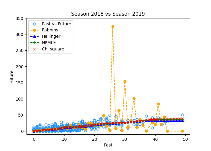
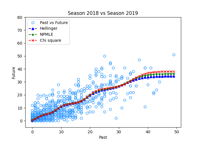
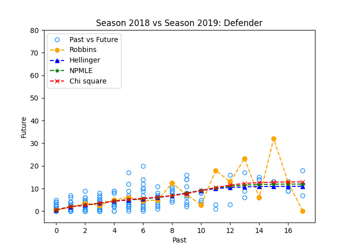
We study the data on total number of goals scored in the National Hockey League for the seasons 2017-18 and 2018-19 (the data is available at https://www.hockey-reference.com/). We consider the statistics of $n=745$ players, for whom the data were collected for both the seasons. Let $Y_{i}$ be the total number of goal scored by the $i^{\text{th}}$ player in the season 2017-18. We model $Y_{i}$ as independently distributed $\mathrm{Poi}(\theta_{i})$, where $\theta_{i}$’s are independently distributed according to some prior $G$ on $\mathbb{R}_{+}$. Based on the observations we intend to predict the goal scored by each player in the season 2018-19. Specifically, for the $i^{\text{th}}$ player our prediction is $\widehat{\theta}(Y_{i})$, where $\widehat{\theta}$ is an empirical Bayes estimator driven by the 2017-18 data, either through $f$-modeling (e.g. $\widehat{\theta}=\widehat{\theta}_{\text{Robbins}}$) or $g$-modeling (e.g. $\widehat{\theta}=\widehat{\theta}_{\widehat{G}}$, where $\widehat{G}$ is learned by minimum-distance methods.) In Fig. 2 we plot the EB estimators based on the Robbins method, the minimum $H^{2}$, the minimum-$\chi^{2}$ distance estimator and the NPMLE against the 2017-18 data (denoted as “Past” on the $x$-axis) and compare their estimates against the real values of goals in 2018-19 (denoted by “Future” on the $y$-axis).

Figure 2: Prediction of hockey goals with empirical Bayes, comparing Robbins and minimum-distance estimators. On the right panel, the Robbins estimator is omitted.

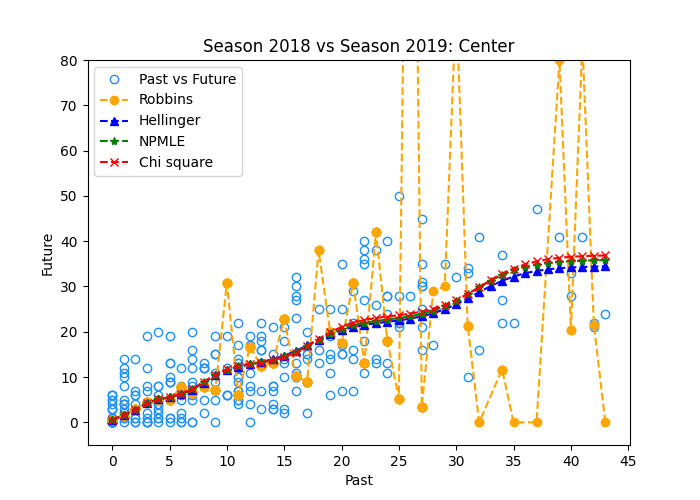
The left panel shows that there exists a large number of individuals for whom the Robbins estimator produces unstable prediction that is significantly worse than all minimum-distance methods. This difference is significant for values of scored goals which have lower sample representations. Thus on the right panel we omit the Robbins estimator and provide a more detailed comparison for the three minimum-distance estimators, which shows that their behavior are mostly comparable except near the tail end of the data-points. Interestingly, all three estimators seem to do shrinkage towards several fixed values. There could be several explanations for this multi-modality. One is that different clusters correspond to different player positions (defense, winger, center). The other is that clusters correspond to the line of the player (different lines get different amount of ice time). To test this hypothesis we also redid on Fig. 3 the estimation for each position separately. Since the multi-modality is retained, we conclude that the second option is more likely to be the real explanation. We also tabulate performance of the estimators in terms of the root mean squared error (RMSE) and the Mean absolute deviation (MAD) with respect to the true goal values in 2018-19:

Methods	Robbins	minimum-$H^{2}$	NPMLE	minimum-$\chi^{2}$
RMSE	15.59	6.02	6.04	6.05
MAD	6.64	4.37	4.38	4.39

Table 1: Robbins vs. minimum-distance: Prediction error comparison.

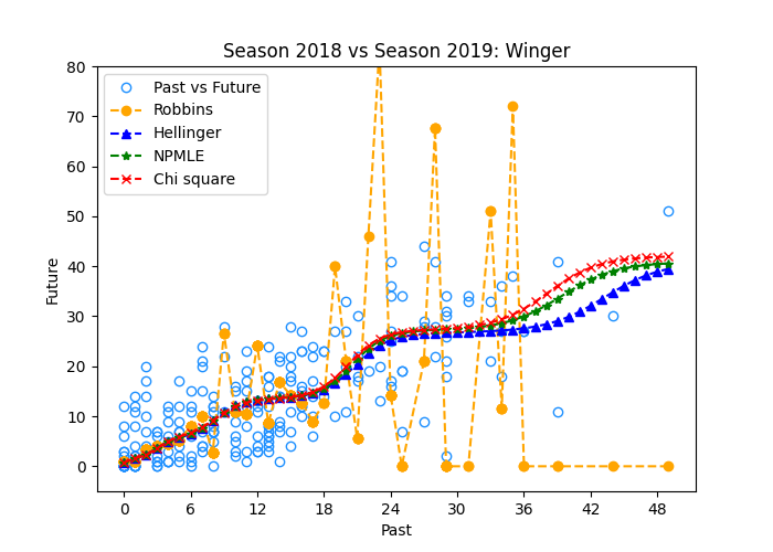
In addition we also compared the four goal-prediction methods based on different EB estimators across the possible playing positions: defender, center, winger. Similar as before, we used the Poisson model and tried to predict the goal scoring for the year 2019 using the goal scoring data from the year 2018 for players in each playing position separately. As expected, the minimum distance methodology provides more stable and accurate estimates that the estimates based on the Robbins method. The plots showing closeness of the predictions to the true number of goals for the different EB methods are provided below.

Figure 3: Prediction of hockey goals at different playing positions.

5.3 More simulation studies

In this subsection, we test more priors in addition to the uniform prior in Fig. 1, including discrete priors and priors with unbounded support. In Section 5.2 we see that the three minimum-distance estimators performed similarly. However, question arises whether the best choice among the minimum-distance EB methods can be argued when some information about the prior is available. With the specific goal of differentiating the three minimum-distance estimators among themselves, we carry out simulation studies in the end of this section using different priors.

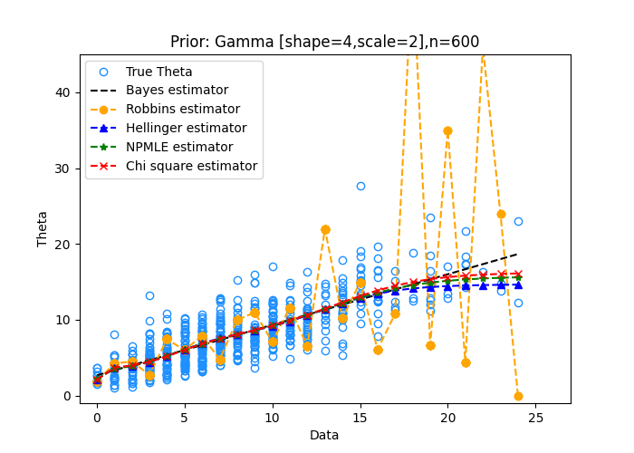
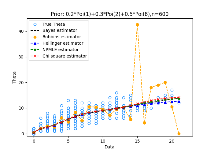
For comparing the EB methods in the discrete setup we choose the prior $G$ to be $0.2\mathrm{Poi}(1)+0.3\mathrm{Poi}(2)+0.5\mathrm{Poi}(8)$ and for the continuous unbounded setup we choose the prior $G$ to be the Gamma distribution with scale parameter 2 and shape parameter 4, i.e. with prior density $f(x)=\frac{1}{96}x^{3}e^{-\frac{x}{2}}$. In both of the cases we simulate $\left\{\theta_{i}\right\}_{i=1}^{600}$ independently from the prior distribution and correspondingly generate data $Y_{i}\sim\mathrm{Poi}(\theta_{i})$. For each of the priors we calculate the Bayes estimator numerically (denoted by the black dashed line in the plots). Then from the generated datasets we compute the Robbins estimator, the NPMLE based EB estimator, the $H^{2}$-distance based EB estimator and the $\chi^{2}$-distance based EB estimator. All the estimators are then plotted against $\theta$ and the data (Fig. 4). As expected, the Robbins estimator shows high deviation from the true $\theta$ values in many instances whereas the minimum-distance based estimators are much more stable.

Figure 4: Robbins vs. minimum-distance estimators: Unbounded priors

To differentiate the different minimum-distance based EB methods we analyze the effect of the tail properties of the prior in the simulations below. Consider the exponential distribution parameterized by scale ($\alpha$) and with density $g_{\alpha}(x)=\frac{1}{\alpha}e^{-x/\alpha}$. Note that the higher values of $\alpha$ generate distributions with heavier tails. We consider three values of $\alpha$: 0.3,1.05 and 2. For each $\alpha$ we estimate the training regret for sample sizes $n$ in the range $[50,300]$. Given sample $Y_{1},\dots,Y_{n}$ from the mixture distribution with prior $G$ we define the training regret for any estimator $\widehat{G}$ of $G$ as $\mathbb{E}_{G}[\frac{1}{n}\sum_{i=1}^{n}(\widehat{\theta}_{G}(Y_{i})-\widehat{\theta}_{\widehat{G}}(Y_{i}))^{2}]$. We compute the Bayes estimator $\widehat{\theta}_{G}(y)$ numerically for each $y$. For every pair $(\alpha,n)$ we replicate the following experiment independently 10,000 times for each minimum-distance method:

• Generate $\{\theta_{i}\}_{i=1}^{n}$ and $Y_{i}\sim\mathrm{Poi}(\theta_{i})$,

• Calculate ${\widehat{G}}$ using minimum-distance method,

• Calculate prediction error $\textsf{E}(Y^{n})=\frac{1}{n}\sum_{i=1}^{n}(\widehat{\theta}_{G}(Y_{i})-\widehat{\theta}_{\widehat{G}}(Y_{i}))^{2}$.

Then we take the average of $\textsf{E}(Y^{n})$ values from all the 10,000 replications to estimate the training error. For each $\alpha$ and each minimum distance method, at every $n$ we also estimate the $95\%$ confidence interval as $[\overline{\textsf{E}(Y^{n})}\mp 0.0196*\textsf{sd}(\textsf{E}(Y^{n}))]$ where $\overline{\textsf{E}(Y^{n})}$ and $\textsf{sd}(\textsf{E}(Y^{n}))$ define respectively the sample mean and the sample standard deviation of the $\textsf{E}(Y^{n})$ values over the 10,000 independent runs. Below we plot the training regrets and their 95% confidence bands against the training sample sizes (Fig. 5).

Figure 5: Comparison of minimum-distance estimators

We observe that that minimum-$H^{2}$ based estimator outperforms the other estimators when the scale of the exponential distribution is small. As the tails of the prior distributions become heavier, the performance of the minimum-$H^{2}$ based estimator gets worse and the NPMLE based estimator comes out as a better choice.

Appendix A Proof of Theorem 1

We first prove the result for the constrained solution $\mathop{\rm argmin}_{Q\in{\mathcal{P}}([0,h])}d(p\|f_{Q})$. As mentioned towards the end of the proof, this also implies the desired result for the unconstrained solution. Suppose that $p$ is supported on $\{y_{1},\dots,y_{m}\}\subset\mathbb{Z}_{+}$. Define

$$S\triangleq\left\{(f_{Q}(y_{1}),\dots,f_{Q}(y_{m})):Q\in{\mathcal{P}}([0,h])\right\},$$ (29)

where $f_{Q}(y)=\mathbb{E}_{\theta\sim Q}[f_{\theta}(y)]$ is the probability mass function of the Poisson mixture (1), and $f_{\theta}(y)=e^{-\theta}\theta^{y}/y!$. We claim that $S$ is convex and compact. The convexity follows from definition. For compactness, note that $S$ is bounded since $\sup_{\theta\geq 0}f_{\theta}(y)=e^{-y}y^{y}/y!$, so it suffices to check $S$ is closed. Let $(f_{1}^{\prime},\ldots,f_{m}^{\prime})\in\mathbb{R}_{+}^{m}$ be the limiting point of $(f_{Q_{k}}(y_{1}),\dots,f_{Q_{k}}(y_{m}))$ for some sequence $\{Q_{k}\}$ in ${\mathcal{P}}([0,h])$. By Prokhorov’s theorem, there is a subsequence $\{Q_{k_{\ell}}\}$ that converges weakly to some $Q^{\prime}\in{\mathcal{P}}([0,h])$. Since $\theta\mapsto f_{\theta}(y)$ is continuous and bounded, we have $f_{j}^{\prime}=f_{Q^{\prime}}(y_{j})$ for all $j$. In other words, $S$ is closed.

Next, define $v:S\to\mathbb{R}$ by $v(f_{1},\dots,f_{m})=\sum_{i=1}^{m}{\ell(p(y_{i}),f_{i})}$. By Assumption 1, the value of the min-distance optimization can be written as

$$\min_{Q\in{\mathcal{P}}([0,h])}d(p\|f_{Q})=t(p)+\min_{(f_{1},\ldots,f_{m})\in S}v(f_{1},\ldots,f_{m}).$$ (30)

Furthermore, by assumption $\ell(0,b)\equiv 0$ and $b\mapsto\ell(a,b)$ is strictly convex for $a>0$. Thus $v$ is strictly convex. Therefore, there exists a unique point $(f_{1}^{*},\dots,f_{m}^{*})\in S$ that achieves the minimum on the right side of (30). Thus, the left side has a minimizer $\widehat{G}\in{\mathcal{P}}([0,h])$ that satisfies

$$f_{\widehat{G}}(y_{j})=f_{j}^{*},j=1,\dots,m$$ (31)

It remains to show that the above representation is unique at the special point $(f_{1}^{*},\dots,f_{m}^{*})$; this argument relies on the specific form of the Poisson density. Let ${\widehat{G}}$ be one such minimizer. By the first-order optimality condition (see (28) in Section 5.1),

$$D_{\widehat{G}}(\theta) =\sum_{i=1}^{m}a_{i}(f_{\theta}(y_{i})-f_{i}^{*})\geq 0,\quad\forall 0\leq\theta\leq h;$$

$$D_{\widehat{G}}(\theta) =0,\quad\text{for $\widehat{G}$-almost every $\theta$},$$ (32)

where $a_{i}\triangleq\frac{d}{df}\ell(p(y_{i}),f)|_{f=f_{i}^{*}}<0$, since $\ell$ is strictly decreasing in the second coordinate and $f_{i}^{*}>0$. Define

$$b_{i}={a_{i}\over\sum_{i=1}^{m}a_{i}f_{i}^{*}}>0.$$

As $\ell$ is strictly decreasing in second coordinate, $\frac{d}{df}\ell(p(y_{i}),f)<0$ for all $f\in\mathbb{R}_{+},i=1,\dots,m$. Using this, we rearrange (A) to get

$$\sum_{i=1}^{m}{b_{i}\over y_{i}!}\theta^{y_{i}} \leq e^{\theta},\forall\theta\in[0,h],$$

$$\sum_{i=1}^{m}{b_{i}\over y_{i}!}\theta^{y_{i}} =e^{\theta}\text{ for each $\theta$ in the support of }\widehat{G}.$$ (33)

Then the following lemma shows that the support of $\widehat{G}$ has at most $m$ points.

Lemma 5.

Suppose that $\sum_{i=1}^{m}\beta_{i}\theta^{y_{i}}\leq e^{\theta}$ for all $\theta\in[0,h]$ where $\beta_{i}\in\mathbb{R}$ and $h>0$. Then the number of solutions to $\sum_{i=1}^{m}\beta_{i}\theta^{y_{i}}=e^{\theta}$ in $\theta\in[0,h]$ is at most $m$.

Proof.

The proof is a modification of [Sim76, Lemma 3.1(2)], which deals with the specific case $h=\infty$. Recall the following version of Descartes’ rule of signs [PS98, Part V, Problem 38 and 40]: Consider an entire function (i.e., a power series whose radius of convergence is infinity) $\phi(x)=a_{0}+a_{1}x+a_{2}x^{2}+\dots$ with real coefficients. Let $r$ be the number of strictly positive zeros of $\phi$ counted with their multiplicities and let $s$ be the number of sign changes in the sequence $a_{0},a_{1},\dots$. Then $r\leq s$. We apply this fact to the function

$$\phi(\theta)=\sum_{i=1}^{m}\beta_{i}\theta^{y_{i}}-e^{\theta}=\sum_{j=0}^{\infty}a_{j}\theta^{j},$$

where

$$a_{j}=\begin{cases}\beta_{i}-\frac{1}{y_{i}!}&j=y_{i},i=1,\dots,m\\ -\frac{1}{j!}<0&\text{else}\\ \end{cases}$$

Case 1:

Suppose that 0 is a root of $\phi(\cdot)$. Then $a_{0}=0$. As there are at most $m-1$ positive coefficients in $a_{0},a_{1},\dots$, there can be at most $2(m-1)$ sign changes, which implies at most $2(m-1)$ positive roots of $s$ counting multiplicities. Note that, as $\phi(\theta){\mathbf{1}_{\left\{{\theta\in(0,h)}\right\}}}\leq 0$ and $s$ is an entire function, each root of $s$ inside $(0,h)$ has multiplicity at least 2. Suppose that $m_{h}$ is the multiplicity of $h$ as a root of $\phi(\cdot)$, which we define to be 0 when $h$ is not a root. This means that the total number of distinct roots in $(0,h)$ is at most the largest integer before $(2(m-1)-m_{h})/2$. If $h$ is not a root then the number distinct roots in $(0,h)$ is at most $m-1$. If $h$ is a root, then its multiplicity is at least 1, and hence, the number of distinct roots in $(0,h)$ is at most $m-2$. Hence, there are at most $m$ many distinct roots in $[0,h]$.

Case 2:

Suppose that 0 is not a root of $\phi(\cdot)$. As there are at most $m$ positive coefficients in $a_{0},a_{1},\dots$, there can be at most $2m$ sign changes, which implies at most $2m$ positive roots counting multiplicities. By a similar argument as in the previous case, the total number of distinct roots in $(0,h)$ is at most than the largest integer before $(2m-m_{h})/2$. If $h$ is not a root then the number distinct roots in $(0,h)$ is at most $m$. If $h$ is a root, then the number of distinct roots in $(0,h)$ is at most $m-1$. Hence, in total at most $m$ distinct roots in $[0,h]$. ∎ Suppose that there are $r(\leq m)$ different $\theta_{i}$’s (denote them by $\theta_{1}\dots,\theta_{r}$) for which (A) holds. This implies given any optimizer ${\widehat{G}}$ its atoms form a subset of $\left\{\theta_{1}\dots,\theta_{r}\right\}$. Let $w_{j}$ be the weight ${\widehat{G}}$ puts on $\theta_{j}$. Then in view of (31) we get that

$$\sum_{j=1}^{r}{w_{j}e^{-\theta_{j}}}\theta_{j}^{y_{i}}=f_{i}^{*}y_{i}!,\quad i=1,\dots,r.$$

The matrix $\{\theta_{j}^{y_{i}}:j=1,\dots,r,i=1,\dots,m\}$ has full column rank, and hence the vector $(w_{1},\dots,w_{r})$ can be solve uniquely. This implies uniqueness of the optimizer ${\widehat{G}}$ as well. This finishes the proof for the constrained solution.

Next we argue for the unconstrained minimizer $\mathop{\rm argmin}_{Q}d(p\|f_{Q})$. In view of Lemma 6 below, we get that the unconstrained minimum-distance estimator is supported on $[0,h]$ with $h=\max_{i=1,\dots,m}y_{i}$. Then from the above proof for $\mathop{\rm argmin}_{Q\in{\mathcal{P}}([0,h])}d(p\|f_{Q})$ the existence and uniqueness of the unconstrained estimator follow.

Lemma 6.

Let $d$ satisfy Assumption 1 and let $p$ be a probability distribution on $\mathbb{Z}_{+}$ with support $\{y_{1},\dots,y_{m}\}$. Then the minimizer $\mathop{\rm argmin}_{Q}d(p\|f_{Q})$ is supported on the interval $[y_{\min},y_{\max}]$, where $y_{\min}=\min_{i=1,\dots,m}y_{i},y_{\max}=\max_{i=1,\dots,m}y_{i}$.

Proof.

Let $Q$ be a distribution with $Q([0,y_{\min}))+Q((y_{\max},\infty))>0$. Define another distribution $\widetilde{Q}$ by

$$\widetilde{Q}(\cdot)=Q([0,y_{\min}))\delta_{y_{\min}}(\cdot)+Q(\cdot\cap[y_{\min},y_{\max}])+Q((y_{\max},\infty))\delta_{y_{\max}}(\cdot).$$

In other words, $\widetilde{Q}$ moves the masses of $Q$ on the intervals $[0,y_{\min})$ (resp. $(y_{\max},\infty)$) to the point $y_{\min}$ (resp. $y_{\max}$). As $f_{\theta}(y)$ is strictly increasing in $\theta\in[0,y)$ and strictly decreasing in $\theta\in(y,\infty)$ we get for each $i=1,\dots,n$

$$f_{Q}(y_{i}) =\int f_{\theta}(y_{i})dQ(\theta)$$

$$=\int_{0\leq\theta<y_{\min}}f_{\theta}(y_{i})dQ(\theta)+\int_{y_{\min}\leq\theta\leq y_{\max}}f_{\theta}(y_{i})dQ(\theta)+\int_{y_{\max}>\theta}f_{\theta}(y_{i})dQ(\theta)$$

$$<Q([0,y_{\min}))f_{y_{\min}}(y_{i})+\int_{y_{\min}\leq\theta\leq y_{\max}}f_{\theta}(y_{i})dQ(\theta)+Q((y_{\max},\infty))f_{y_{\max}}(y_{i})$$

$$=\int f_{\theta}(y_{i})d\widetilde{Q}(\theta)=f_{\widetilde{Q}}(y_{i}).$$

Hence, by Assumption 1, we get

$$d(p\|f_{Q}) =t(p)+\sum_{y:p(y)>0}\ell(p(y),f_{Q}(y))$$

$$\overset{\rm(a)}{=}t(p)+\sum_{y:p(y)>0}{\ell(p(y),f_{Q}(y))}\overset{\rm(b)}{>}t(p)+\sum_{y:p(y)>0}{\ell\left(p(y),f_{\widetilde{Q}}(y)\right)}=d(p\|f_{\widetilde{Q}}),$$ (34)

where (a) follows from $\ell(0,\cdot)=0$; (b) follows as the function $b\mapsto\ell(a,b)$ is strictly decreasing. In other words, given any $Q$ with $Q([0,y_{\min}))+Q((y_{\max},\infty))>0$ we can produce $\widetilde{Q}$ supported on $[y_{\min},y_{\max}]$ such that $d(p\|f_{\widetilde{Q}})<d(p\|f_{Q})$. Hence, the claim follows. ∎

Appendix B Proof of Lemma 4

Let $\theta\sim G,Y|\theta\sim f_{\theta}$. Then for any $\widehat{G}$ independent of $Y$, we can write $\mathsf{Regret}(\widehat{G};G)=\sum_{y=0}^{\infty}(\widehat{\theta}_{\widehat{G}}(y)-\widehat{\theta}_{G}(y))^{2}f_{G}(y)=\mathbb{E}_{G}\left[\left(\widehat{\theta}_{{\widehat{G}}}(Y)-\widehat{\theta}_{G}(Y)\right)^{2}\right]$; cf. (10). Fix $h>0$ and note the following

• $\text{mmse}({G_{h}})\leq{\text{mmse}(G)\over G([0,h])}$ [WV10, Lemma 2],

• $\text{mmse}(G)\leq\sqrt{\mathbb{E}_{G}[\theta^{4}]}\leq\sqrt{M}$, and

• For any fixed distribution $\widehat{G}$

  $$\mathbb{E}_{G}\left[(\widehat{\theta}_{{{\widehat{G}}}}(Y)-\theta)^{2}\right] \leq\mathbb{E}_{G}\left[(\widehat{\theta}_{{{\widehat{G}}}}(Y)-\theta)^{2}{\mathbf{1}_{\left\{{\theta\leq h}\right\}}}\right]+\mathbb{E}_{G}\left[(\widehat{\theta}_{{{\widehat{G}}}}(Y)-\theta)^{2}{\mathbf{1}_{\left\{{\theta>h}\right\}}}\right]$$

  $$\overset{\rm(a)}{\leq}\mathbb{E}_{G}\left[\left.(\widehat{\theta}_{{{\widehat{G}}}}(Y)-\theta)^{2}\right|{\theta\leq h}\right]+\sqrt{\mathbb{E}_{G}\left[(\widehat{\theta}_{{{\widehat{G}}}}(Y)-\theta)^{4}\right]\mathbb{E}_{G}\left[{\mathbf{1}_{\left\{{\theta>h}\right\}}}\right]}$$

  $$\overset{\rm(b)}{\leq}\mathbb{E}_{G_{h}}\left[(\widehat{\theta}_{{{\widehat{G}}}}(Y)-\theta)^{2}\right]+\sqrt{8(\widehat{h}^{4}+\mathbb{E}_{G}[\theta^{4}])G((h,\infty))}$$

  $$=\mathbb{E}_{G_{h}}\left[(\widehat{\theta}_{{{\widehat{G}}}}(Y)-\theta)^{2}\right]+\sqrt{8(\widehat{h}^{4}+M)G((h,\infty))}.$$

  where step (a) followed by Cauchy-Schwarz inequality and step (b) followed as $(x+y)^{4}\leq 8(x^{4}+y^{4})$ for any $x,y\in\mathbb{R}$.

Using these we get

$$\mathsf{Regret}(\widehat{G};G) =\mathbb{E}_{G}\left[(\widehat{\theta}_{{{\widehat{G}}}}(Y)-\theta)^{2}\right]-\text{mmse}(G)$$

$$\leq\mathbb{E}_{G_{h}}\left[(\widehat{\theta}_{{{\widehat{G}}}}(Y)-\theta)^{2}\right]-\text{mmse}(G_{h})+\text{mmse}({G_{h}})-\text{mmse}(G)+\sqrt{8(\widehat{h}^{4}+M)G((h,\infty))}$$

$$\leq\mathbb{E}_{G_{h}}\left[(\widehat{\theta}_{{{\widehat{G}}}}(Y)-\widehat{\theta}_{G_{h}}(Y))^{2}\right]+\left(\frac{1}{G([0,h])}-1\right){\text{mmse}(G)}+\sqrt{8(\widehat{h}^{4}+M)G((h,\infty))}$$

$$\leq\mathbb{E}_{G_{h}}\left[(\widehat{\theta}_{{{\widehat{G}}}}(Y)-\widehat{\theta}_{G_{h}}(Y))^{2}\right]+{\frac{G((h,\infty))}{G([0,h])}}\sqrt{M}+\sqrt{8(\widehat{h}^{4}+M)G((h,\infty))}$$

$$\leq\mathbb{E}_{G_{h}}\left[(\widehat{\theta}_{{{\widehat{G}}}}(Y)-\widehat{\theta}_{G_{h}}(Y))^{2}\right]+{(1+2\sqrt{2})\sqrt{(\widehat{h}^{4}+M)G((h,\infty))}\over G([0,h])}.$$ (35)

Next we bound the first term. Fix $K\geq 1$. Using $\widehat{\theta}_{{G_{h}}}(y)\leq h,\widehat{\theta}_{\widehat{G}}(y)\leq\widehat{h}$ we have

$$\mathbb{E}_{G_{h}}\left[(\widehat{\theta}_{\widehat{G}}(Y)-\widehat{\theta}_{{G}_{h}}(Y))^{2}{\mathbf{1}_{\left\{{Y\leq K-1}\right\}}}\right]$$

$$=\sum_{y=0}^{K-1}(y+1)^{2}f_{G_{h}}(y)\left({f_{\widehat{G}}(y+1)\over f_{\widehat{G}}(y)}-{f_{G_{h}}(y+1)\over f_{G_{h}}(y)}\right)^{2}$$

$$\overset{\rm(a)}{\leq}\sum_{y=0}^{K-1}(y+1)^{2}f_{G_{h}}(y)\left\{3\left({f_{\widehat{G}}(y+1)\over f_{\widehat{G}}(y)}-{2f_{\widehat{G}}(y+1)\over f_{G_{h}}(y)+f_{\widehat{G}}(y)}\right)^{2}+3\left({f_{G_{h}}(y+1)\over f_{G_{h}}(y)}-{2f_{G_{h}}(y+1)\over f_{G_{h}}(y)+f_{\widehat{G}}(y)}\right)^{2}\right.$$

$$\quad\left.+3\left(2f_{G_{h}}(y+1)-2f_{\widehat{G}}(y+1)\over f_{G_{h}}(y)+f_{\widehat{G}}(y)\right)^{2}\right\}$$

$$\leq 3\sum_{y=0}^{K-1}\left\{\left((y+1)f_{\widehat{G}}(y+1)\over f_{\widehat{G}}(y)\right)^{2}{(f_{G_{h}}(y)-f_{\widehat{G}}(y))^{2}\over f_{G_{h}}(y)+f_{\widehat{G}}(y)}+\left((y+1)f_{G_{h}}(y+1)\over f_{G_{h}}(y)\right)^{2}{(f_{G_{h}}(y)-f_{\widehat{G}}(y))^{2}\over f_{G_{h}}(y)+f_{\widehat{G}}(y)}\right.$$

$$\quad\left.+4(y+1)^{2}{(f_{G_{h}}(y+1)-f_{\widehat{G}}(y+1))^{2}\over f_{G_{h}}(y)+f_{\widehat{G}}(y)}\right\}$$

$$=3(\{\widehat{\theta}_{G_{h}}(y)\}^{2}+\{\widehat{\theta}_{\widehat{G}}(y)\}^{2})\sum_{y=0}^{K-1}{(f_{G_{h}}(y)-f_{\widehat{G}}(y))^{2}\over f_{G_{h}}(y)+f_{\widehat{G}}(y)}+12\sum_{y=0}^{K-1}(y+1)^{2}{(f_{G_{h}}(y+1)-f_{\widehat{G}}(y+1))^{2}\over f_{G_{h}}(y)+f_{\widehat{G}}(y)}$$

$$\leq 3(h^{2}+\widehat{h}^{2})\sum_{y=0}^{K-1}{(f_{G_{h}}(y)-f_{\widehat{G}}(y))^{2}\over f_{G_{h}}(y)+f_{\widehat{G}}(y)}+12\sum_{y=0}^{K-1}(y+1)^{2}{(f_{G_{h}}(y+1)-f_{\widehat{G}}(y+1))^{2}\over f_{G_{h}}(y)+f_{\widehat{G}}(y)}$$

where (a) followed from $(x+y+z)^{2}\leq 3(x^{2}+y^{2}+z^{2})$ for any $x,y,z\in\mathbb{R}$. Using $(\sqrt{f_{G_{h}}(x)}+\sqrt{f_{\widehat{G}}(x)})^{2}\leq 2(f_{G_{h}}(x)+f_{\widehat{G}}(x))$ for $x=y,y+1$ we continue the last display to get

$$\mathbb{E}_{G_{h}}\left[(\widehat{\theta}_{{\widehat{G}}}(Y)-\widehat{\theta}_{G_{h}}(Y))^{2}{\mathbf{1}_{\left\{{Y\leq K-1}\right\}}}\right]$$

$$\leq 6(h^{2}+\widehat{h}^{2})\sum_{y=0}^{K-1}(\sqrt{f_{G_{h}}(y)}-\sqrt{f_{\widehat{G}}(y)})^{2}$$

$$\quad+24K\max_{y=0}^{K-1}{(y+1)f_{G_{h}}(y+1)+(y+1)f_{\widehat{G}}(y+1)\over f_{G_{h}}(y)+f_{\widehat{G}}(y)}\sum_{y=0}^{K-1}(\sqrt{f_{G_{h}}(y+1)}-\sqrt{f_{\widehat{G}}(y+1)})^{2}$$

$$\leq\left(6(h^{2}+\widehat{h}^{2})+24(h+\widehat{h})K\right){H^{2}(f_{\widehat{G}},f_{G_{h}})}.$$

Again using $\widehat{\theta}_{{G_{h}}}(y)\leq h,\widehat{\theta}_{\widehat{G}}(y)\leq\widehat{h}$ we bound $\mathbb{E}_{G_{h}}\left[(\widehat{\theta}_{{\widehat{G}}}(Y)-\widehat{\theta}_{G_{h}}(Y))^{2}{\mathbf{1}_{\left\{{Y\geq K}\right\}}}\right]$ by $(h+\widehat{h})^{2}\epsilon_{K}(G_{h})$. Combining this with the last display we get

$$\mathbb{E}_{G_{h}}\left[(\widehat{\theta}_{{\widehat{G}}}(Y)-\widehat{\theta}_{G_{h}}(Y))^{2}\right]\leq\left\{6(h^{2}+\widehat{h}^{2})+24(h+\widehat{h})K\right\}{H^{2}(f_{\widehat{G}},f_{G_{h}})}+(h+\widehat{h})^{2}\epsilon_{K}(G_{h}).$$

In view of above continuing (B) we have

$$\mathsf{Regret}(\widehat{G};G)\leq \left\{6(h^{2}+\widehat{h}^{2})+24(h+\widehat{h})K\right\}{H^{2}(f_{\widehat{G}},f_{G_{h}})}$$

$$\quad+(h+\widehat{h})^{2}\epsilon_{K}(G_{h})+{(1+2\sqrt{2})\sqrt{(M+\widehat{h}^{4})G((h,\infty))}\over G([0,h])}.$$ (36)

Using triangle inequality and $(x+y)^{2}\leq 2(x^{2}+y^{2})$ we get

$$H^{2}(f_{{\widehat{G}}},f_{G_{h}})\leq 2\left\{H^{2}(f_{G},f_{{\widehat{G}}})+H^{2}(f_{G_{h}},f_{G})\right\}.$$ (37)

Note that

$$H^{2}(f_{G_{h}},f_{G})\leq 2{\rm TV}(f_{G_{h}},f_{G})\leq 2{\rm TV}(G_{h},G)=2G((h,\infty)).$$

where ${\rm TV}$ denotes the total variation and the middle inequality applies the data-processing inequality [Csi67].

Then, combining (36), (37) and (21) we get

$$\mathsf{Regret}(\widehat{G};G) \leq\left\{12(h^{2}+\widehat{h}^{2})+48(h+\widehat{h})K\right\}\left(H^{2}(f_{\widehat{G}},f_{G})+2G((h,\infty))\right)$$

$$\quad+(h+\widehat{h})^{2}{\epsilon_{K}(G)\over G([0,h])}+{(1+2\sqrt{2})\sqrt{(M+\widehat{h}^{4})G((h,\infty))}\over G([0,h])}$$

This finishes the proof.

Appendix C Auxiliary results

Given any $s>0$ and $G\in\mathsf{SubE}(s)$, the following are satisfied.

1. If $\theta\sim{G}$, then $\mathbb{E}[\theta^{4}]\leq 30s^{4}$.

2. If $\left\{Y_{i}\right\}_{i=1}^{n}{\stackrel{{\scriptstyle\text{i.i.d.}}}{{\sim}}}f_{G}$, then

   $$\mathbb{P}\left[Y_{1}\geq K\right]\leq\frac{3}{2}e^{-K\log\left(1+\frac{1}{2s}\right)},\quad\mathbb{E}\left[Y_{\max}^{4}\right]\leq{64(\log n)^{4}+45\over\left(\log\left(1+\frac{1}{2s}\right)\right)^{4}}.$$ (38)

To prove (i) we note that $z^{3}\leq 15e^{\frac{z}{2}},z\in\mathbb{R}$. Then we have

$$\mathbb{E}[\theta^{4}]=4\int y^{3}\mathbb{P}\left[\theta>y\right]dy\leq 2\int y^{3}e^{-\frac{y}{s}}dy\leq 30s^{4}\int e^{-\frac{z}{2}}dz\leq 30s^{4}.$$

The proof of the property (ii) is as follows. Using $\mathbb{E}_{Z\sim\mathrm{Poi}(\theta)}\left[e^{Zt}\right]=e^{\theta(e^{t}-1)},t>0$ and denoting $c(s)=\log{1+2s\over 2s}$ we have

$$\mathbb{E}\left[e^{Y_{1}c(s)}\right]=\mathbb{E}_{\theta\sim{G}}\left[\mathbb{E}_{Y_{1}\sim\mathrm{Poi}(\theta)}\left[\left.e^{Y_{1}c(s)}\right|\theta\right]\right]=\mathbb{E}_{G}\left[e^{\theta\over 2s}\right]=\int e^{\theta/2s}G(d\theta)$$

$$=\int_{\theta}\int_{x<\theta}{e^{x/2s}\over 2s}dxG(d\theta)=\int_{x}{e^{x/2s}\over 2s}G([x,\infty))dx\overset{\rm(a)}{\leq}\int_{x<0}{e^{x/2s}\over 2s}dx+\int_{x>0}{e^{-x/2s}\over s}dx\leq\frac{3}{2}$$

where (a) followed by using tail bound for $\mathsf{SubE}(s)$ distribution $G$. In view of Markov inequality

$$\mathbb{P}\left[Y_{1}\geq K\right]\leq\mathbb{E}\left[e^{Y_{1}c(s)}\right]e^{-c(s)K}\leq\frac{3}{2}e^{-K\log\left(1+\frac{1}{2s}\right)}.$$ (39)

For the expectation term we have for any $L>0$

$$\mathbb{E}\left[\left(Y_{\max}\right)^{4}\right] =4\int y^{3}\mathbb{P}\left[Y_{\max}>y\right]$$

$$\leq 4L^{4}+n\int_{y>L}y^{3}\mathbb{P}\left[Y_{1}>y\right]dy$$

$$\leq 4L^{4}+{3n\over 2}\int_{y>L}y^{3}e^{-y\log\left(1+\frac{1}{2s}\right)}dy$$

$$\leq 4L^{4}+\frac{3n}{2\left\{\log\left(1+\frac{1}{2s}\right)\right\}^{4}}\int_{z>L\log\left(1+\frac{1}{2s}\right)}z^{3}e^{-z}dz$$

$$\leq 4L^{4}+\frac{45n}{2\left\{\log\left(1+\frac{1}{2s}\right)\right\}^{4}}\int_{z>L\log\left(1+\frac{1}{2s}\right)}e^{-z/2}dz\leq 4L^{4}+{45ne^{-\frac{L}{2}\log\left(1+\frac{1}{2s}\right)}\over\left\{\log\left(1+\frac{1}{2s}\right)\right\}^{4}}.$$

Choosing $L={2\log n\over\log\left(1+\frac{1}{2s}\right)}$ we get the desired result.

References

• [Ber55] Joseph Berkson. Maximum likelihood and minimum χ2superscript𝜒2\chi^{2} estimates of the logistic function. Journal of the American statistical association, 50(269):130–162, 1955.
• [Ber77] Rudolf Beran. Minimum Hellinger distance estimates for parametric models. The annals of Statistics, pages 445–463, 1977.
• [BG09] Lawrence D Brown and Eitan Greenshtein. Nonparametric empirical Bayes and compound decision approaches to estimation of a high-dimensional vector of normal means. The Annals of Statistics, pages 1685–1704, 2009.
• [BGR13] Lawrence D Brown, Eitan Greenshtein, and Ya’acov Ritov. The poisson compound decision problem revisited. Journal of the American Statistical Association, 108(502):741–749, 2013.
• [BM72] G Kemble Bennett and HF Martz. A continuous empirical Bayes smoothing technique. Biometrika, 59(2):361–368, 1972.
• [Bol77] E Bolthausen. Convergence in distribution of minimum-distance estimators. Metrika, 24(1):215–227, 1977.
• [Bro08] Lawrence D Brown. In-season prediction of batting averages: A field test of empirical Bayes and Bayes methodologies. The Annals of Applied Statistics, 2(1):113–152, 2008.
• [Cas85] George Casella. An introduction to empirical Bayes data analysis. The American Statistician, 39(2):83–87, 1985.
• [Che95] Jiahua Chen. Optimal rate of convergence for finite mixture models. The Annals of Statistics, 23:221–233, 1995.
• [Che17] Jiahua Chen. Consistency of the MLE under mixture models. Statistical Science, 32(1):47–63, 2017.
• [Csi67] I. Csiszár. Information-type measures of difference of probability distributions and indirect observations. Studia Sci. Math. Hungar., 2:299–318, 1967.
• [DK68] JJ Deely and RL Kruse. Construction of sequences estimating the mixing distribution. The Annals of Mathematical Statistics, 39(1):286–288, 1968.
• [Ede88] David Edelman. Estimation of the mixing distribution for a normal mean with applications to the compound decision problem. The Annals of Statistics, 16(4):1609–1622, 1988.
• [Efr14] Bradley Efron. Two modeling strategies for empirical Bayes estimation. Statistical science: a review journal of the Institute of Mathematical Statistics, 29(2):285, 2014.
• [Efr21] Bradley Efron. Empirical Bayes: Concepts and Methods. 2021. http://statweb.stanford.edu/~ckirby/brad/papers/2021EB-concepts-methods.pdf.
• [EH21] Bradley Efron and Trevor Hastie. Computer Age Statistical Inference, Student Edition: Algorithms, Evidence, and Data Science, volume 6. Cambridge University Press, 2021.
• [ETST01] Bradley Efron, Robert Tibshirani, John D Storey, and Virginia Tusher. Empirical Bayes analysis of a microarray experiment. Journal of the American statistical association, 96(456):1151–1160, 2001.
• [Fed72] Valerii Vadimovich Fedorov. Theory of optimal experiments. Elsevier, 1972.
• [GvdV01] S. Ghosal and A.W. van der Vaart. Entropies and rates of convergence for maximum likelihood and Bayes estimation for mixtures of normal densities. The Annals of Statistics, 29(5):1233–1263, 2001.
• [HK18] Philippe Heinrich and Jonas Kahn. Strong identifiability and optimal minimax rates for finite mixture estimation. The Annals of Statistics, 46(6A):2844–2870, 2018.
• [HS83] JC van Houwelingen and Th Stijnen. Monotone empirical Bayes estimators for the continuous one-parameter exponential family. Statistica Neerlandica, 37(1):29–43, 1983.
• [HS84] James Heckman and Burton Singer. A method for minimizing the impact of distributional assumptions in econometric models for duration data. Econometrica: Journal of the Econometric Society, pages 271–320, 1984.
• [Jew82] Nicholas P Jewell. Mixtures of exponential distributions. The annals of statistics, pages 479–484, 1982.
• [JZ09] Wenhua Jiang and Cun-Hui Zhang. General maximum likelihood empirical Bayes estimation of normal means. The Annals of Statistics, 37(4):1647–1684, 2009.
• [KG17] Roger Koenker and Jiaying Gu. Rebayes: an r package for empirical bayes mixture methods. Journal of Statistical Software, 82:1–26, 2017.
• [Kim14] Arlene KH Kim. Minimax bounds for estimation of Normal mixtures. bernoulli, 20(4):1802–1818, 2014.
• [KM14] Roger Koenker and Ivan Mizera. Convex optimization, shape constraints, compound decisions, and empirical Bayes rules. Journal of the American Statistical Association, 109(506):674–685, 2014.
• [KW56] Jack Kiefer and Jacob Wolfowitz. Consistency of the maximum likelihood estimator in the presence of infinitely many incidental parameters. The Annals of Mathematical Statistics, pages 887–906, 1956.
• [Lai82] Nan M Laird. Empirical Bayes estimates using the nonparametric maximum likelihood estimate for the prior. Journal of Statistical Computation and Simulation, 15(2-3):211–220, 1982.
• [LGL05] Jianjun Li, Shanti S Gupta, and Friedrich Liese. Convergence rates of empirical Bayes estimation in exponential family. Journal of statistical planning and inference, 131(1):101–115, 2005.
• [Lin83a] Bruce G Lindsay. The geometry of mixture likelihoods: a general theory. The annals of statistics, pages 86–94, 1983.
• [Lin83b] Bruce G Lindsay. The geometry of mixture likelihoods, part II: the Exponential family. The Annals of Statistics, 11(3):783–792, 1983.
• [Lin95] Bruce G Lindsay. Mixture models: theory, geometry and applications. In NSF-CBMS regional conference series in probability and statistics, pages i–163. JSTOR, 1995.
• [LK69] Glen H Lemon and Richard G Krutchkoff. An empirical Bayes smoothing technique. Biometrika, 56(2):361–365, 1969.
• [LT84] Diane Lambert and Luke Tierney. Asymptotic properties of maximum likelihood estimates in the mixed Poisson model. The Annals of Statistics, pages 1388–1399, 1984.
• [Mar66] JS Maritz. Smooth empirical Bayes estimation for one-parameter discrete distributions. Biometrika, 53(3-4):417–429, 1966.
• [Mar68] JS Maritz. On the smooth empirical Bayes approach to testing of hypotheses and the compound decision problem. Biometrika, 55(1):83–100, 1968.
• [Mar69] JS Maritz. Empirical bayes estimation for the Poisson distribution. Biometrika, 56(2):349–359, 1969.
• [Mil84] PW Millar. A general approach to the optimality of minimum distance estimators. Transactions of the American Mathematical Society, 286(1):377–418, 1984.
• [MKV+21] Zhen Miao, Weihao Kong, Ramya Korlakai Vinayak, Wei Sun, and Fang Han. Fisher-pitman permutation tests based on nonparametric Poisson mixtures with application to single cell genomics. arXiv preprint arXiv:2106.03022, 2021.
• [ML18] Johannes S Maritz and T Lwin. Empirical Bayes methods. Chapman and Hall/CRC, 2018.
• [Mor83] Carl N Morris. Parametric empirical Bayes inference: theory and applications. Journal of the American statistical Association, 78(381):47–55, 1983.
• [Pfa88] Johann Pfanzagl. Consistency of maximum likelihood estimators for certain nonparametric families, in particular: mixtures. Journal of Statistical Planning and Inference, 19(2):137–158, 1988.
• [PLLB10] Bhagwant Persaud, Bo Lan, Craig Lyon, and Ravi Bhim. Comparison of empirical Bayes and full Bayes approaches for before–after road safety evaluations. Accident Analysis & Prevention, 42(1):38–43, 2010.
• [Pol80] David Pollard. The minimum distance method of testing. Metrika, 27(1):43–70, 1980.
• [PS98] G Pólya and G Szegö. Problems and Theorems in Analysis II,(reprint ed.). Springer, Heidelburg, 1998.
• [PW21] Yury Polyanskiy and Yihong Wu. Sharp regret bounds for empirical Bayes and compound decision problems. arXiv preprint arXiv:2109.03943, 2021.
• [Rob51] Herbert Robbins. Asymptotically subminimax solutions of compound statistical decision problems. In Proceedings of the second Berkeley symposium on mathematical statistics and probability, pages 131–149. University of California Press, 1951.
• [Rob56] Herbert Robbins. An Empirical Bayes Approach to Statistics. In Proceedings of the Third Berkeley Symposium on Mathematical Statistics and Probability, Volume 1: Contributions to the Theory of Statistics. The Regents of the University of California, 1956.
• [Sim76] Leopold Simar. Maximum likelihood estimation of a compound Poisson process. The Annals of Statistics, 4(6):1200–1209, 1976.
• [VH96] Jay M Ver Hoef. Parametric empirical Bayes methods for ecological applications. Ecological Applications, 6(4):1047–1055, 1996.
• [Wol53] J Wolfowitz. Estimation by the minimum distance method. Annals of the Institute of Statistical Mathematics, 5(1):9–23, 1953.
• [Wol54] J Wolfowitz. Estimation by the minimum distance method in nonparametric stochastic difference equations. The Annals of Mathematical Statistics, 25(2):203–217, 1954.
• [Wol57] Jacob Wolfowitz. The minimum distance method. The Annals of Mathematical Statistics, pages 75–88, 1957.
• [WV10] Yihong Wu and Sergio Verdú. Functional properties of MMSE. In 2010 IEEE International Symposium on Information Theory, pages 1453–1457. IEEE, 2010.
• [Wyn70] Henry P Wynn. The sequential generation of d𝑑d-optimum experimental designs. The Annals of Mathematical Statistics, 41(5):1655–1664, 1970.
• [Zha03] Cun-Hui Zhang. Compound decision theory and empirical Bayes methods. Annals of Statistics, pages 379–390, 2003.
• [Zha09] Cun-Hui Zhang. Generalized maximum likelihood estimation of normal mixture densities. Statistica Sinica, pages 1297–1318, 2009.