Soft breaking of the μτ𝜇𝜏\mu\leftrightarrow\tau symmetry by 𝐒4𝐙2tensor-productsubscript𝐒4subscript𝐙2\mathbf{S}_{4}\otimes\mathbf{Z}_{2}

J. D. García-Aguilar jdgarcia@ipn.mx Centro de Estudios Científicos y Tecnológicos No 16, Instituto Politécnico Nacional, Kilómetro 1.500, Actopan - Pachuca, Distrito de Educación, Salud, Ciencia, Tecnología e Innovación, San Agustín Tlaxiaca, Hidalgo; México.    Asahel Enrique Pozas Ramírez apozasr1700@alumno.ipn.mx Escuela Superior de Física y Matemáticas, Instituto Politécnico Nacional, Av. Instituto Politécnico Nacional s/n Edificio 9 Unidad Profesional “Adolfo López Mateos” Col. San Pedro Zacatenco, Alcaldía Gustavo A. Madero, C.P. 07738, Ciudad de México; México.    Marlon Michael Suárez Castañeda msuarezc1700@alumno.ipn.mx Escuela Superior de Física y Matemáticas, Instituto Politécnico Nacional, Av. Instituto Politécnico Nacional s/n Edificio 9 Unidad Profesional “Adolfo López Mateos” Col. San Pedro Zacatenco, Alcaldía Gustavo A. Madero, C.P. 07738, Ciudad de México; México.    Juan Carlos Gómez-Izquierdo cizquierdo@ipn.mx
Centro de Estudios Científicos y Tecnológicos No 16, Instituto Politécnico Nacional, Kilómetro 1.500, Actopan - Pachuca, Distrito de Educación, Salud, Ciencia, Tecnología e Innovación, San Agustín Tlaxiaca, Hidalgo; México.
Abstract

The μτ𝜇𝜏\mu\leftrightarrow\tau symmetry has been ruled out by its predictions on the reactor and atmospheric angles, nevertheless, a breaking of this symmetry might provide correct values. For that reason, we build a non-renormalizable lepton model where the mixings arise from the spontaneous breaking of the 𝐒4𝐙2tensor-productsubscript𝐒4subscript𝐙2\mathbf{S}_{4}\otimes\mathbf{Z}_{2} discrete group, subsequently the μτ𝜇𝜏\mu\leftrightarrow\tau symmetry is broken in the effective neutrino mass matrix, that comes from the type II see-saw mechanism. As main result, the reactor and atmospheric angles are corrected and their values are in good agreement with the experimental data for the inverted hierarchy. Furthermore, we point out a link between the atmospheric angle and reactor one. In the quark sector, under certain assumptions, the generalized Fritzsch textures shape to the quark mass matrices so that the CKM matrix values are guaranteed.

CECyT 16-21-I

I Introduction

The confirmed (g2)μsubscript𝑔2𝜇(g-2)_{\mu} anomaly by the Fermilab [1] and the W𝑊W boson mass new measurement [2], which are not consistent with the theoretical prediction, have shown again that the Standard Model (SM) is incomplete. Along with this, the flavor puzzle remains to be solved so that there is a need to enlarge the SM.

The neutrino oscillation opened the window to search physics beyond the SM, as it is well known, these established that neutrinos have mass so they mix. Although there are many mechanism [3] to get tiny neutrino masses, so far there is no a convincing theory that explains the origin of such mass and the peculiar pattern which is completely different from the quark sector. In the last years, several experiments have measured the neutrino mixing angles with great accuracy, also the masses seem to obey two orderings (normal and inverted hierarchy) due to the lacking of information on the absolute neutrino mass. Certainly, the normal ordering is preferred by the available data [4, 5] but the inverted hierarchy is not completely discarded [6]. Another important point is that, conforming to the experimental data, the PMNS mixing matrix exhibits large values in its entries, in addition, the second and third rows satisfy the relation |𝐔μi|=|𝐔τi|subscript𝐔𝜇𝑖subscript𝐔𝜏𝑖|\mathbf{U}_{\mu i}|=|\mathbf{U}_{\tau i}| (i=1,2,3𝑖123i=1,2,3) in good approximation for the normal and inverted hierarchy. The aforementioned facts might be understood by means of a symmetry in the effective neutrino mass matrix, then the concept of flavor symmetry turn out being crucial to explain the mixings, and a variety of discrete symmetries [7, 8, 9, 10, 11, 8, 12, 13, 14] have been applied to the lepton sector. In particular, the neutrino data seem to obey an approximated μτ𝜇𝜏\mu\leftrightarrow\tau symmetry (for a complete review see [15]), that consists in the exchange label μτ𝜇𝜏\mu\leftrightarrow\tau in the effective neutrino mass matrix when the charged lepton mass one is diagonal. Speaking of exact μτ𝜇𝜏\mu\leftrightarrow\tau symmetry, which is is outdated currently due to its predictions, would imply to obtain 0superscript00^{\circ} and 45superscript4545^{\circ} for the reactor and atmospheric angles, respectively. Besides that, the solar angle and the Dirac CP-violating phase keep as a free and unknown parameters. Despite this, from the model building point of view, the well studied μτ𝜇𝜏\mu\leftrightarrow\tau symmetry has been a guide to construct lepton models [16, 17, 18, 19, 20, 21, 22, 23, 24] and there is a possibility that a soft breaking  [25, 26, 27, 28, 21, 22, 23, 29] of this symmetry can accommodate the experimental results so that there is still strong motivation to study on the μτ𝜇𝜏\mu\leftrightarrow\tau symmetry. Apart from this, elaborated flavored models have been proposed to face the lepton mixings and related issues as leptogenesis, dark matter, and so forth [30, 31, 14].

On the other hand, in the quark sector, according to the available data [32] the CKM matrix is close to the identity one, this pattern might be explained by the notable hierarchy among the quark masses. In addition, this feature is exhibited by some matrices like the nearest neighbor interactions (NNI) [33, 34, 35, 36] and the generalized Fritzsch [37, 38, 39] mass textures which can be obtained by means the flavor symmetries [7, 8, 9, 10]. The contrasting behavior between the PMNS and CKM mixing matrices is undoubtedly a puzzling problem, so far one of the main task for model builders is to match simultaneously the fermion mixings by the same flavor symmetry in the suitable framework.

In order to address the masses and mixing problem, a phenomenological scalar extension of the SM is realized where the type II see-saw mechanism is responsible to obtain small neutrino masses and special emphasis is put on the lepton sector under a soft breaking of the μτ𝜇𝜏\mu\leftrightarrow\tau symmetry scheme. To do so, we use the 𝐒4subscript𝐒4\mathbf{S}_{4}[40, 41, 42, 43, 44, 45, 46, 47, 48] non-abelian discrete group to handle the Yukawa couplings, at the same time, this symmetry allows to treat the quark, lepton and scalar sector in different manner. Additionally, we include a 𝐙2subscript𝐙2\mathbf{Z}_{2} symmetry, to have a non-renormalizable Yukawa mass term for neutrinos. On the other hand, the inclusion of three Higgs doublets are required to obtain the quark and charged lepton masses and mixings, this latter comes out being diagonal as result of the matter assignation under the flavor symmetry. Then, an enriched scalar (flavons) sector is included to provide desirable mass textures. In consequence, the mixings arises from the spontaneous breaking of the 𝐒4𝐙2tensor-productsubscript𝐒4subscript𝐙2\mathbf{S}_{4}\otimes\mathbf{Z}_{2} discrete group and the μτ𝜇𝜏\mu\leftrightarrow\tau symmetry is broken in the effective neutrino mass matrix. Eventually, the reactor and atmospheric angles come out being different of 0superscript00^{\circ} and 45superscript4545^{\circ} respectively. CP parities phases in the neutrino masses play an important role to get sizable values for θ13subscript𝜃13\theta_{13} and the deviation of θ23subscript𝜃23\theta_{23} from maximality which turn out being consistent with neutrino data for the inverted hierarchy. In the quark sector, under certain assumptions, the generalized Fritzsch textures shape to the quark mass matrices so that the CKM matrix values are guaranteed.

It is worthy mentioned that a similar study was carried out [24], nonetheless there are clear differences namely. The first one is scalar matter and the flavor symmetry, the second one is related with the mechanism to generate small neutrino masses and the corresponding predictions: in the aforementioned paper, they got exact μτ𝜇𝜏\mu\leftrightarrow\tau symmetry. Lastly, the NNI textures, in the quark mass matrices, appeared in a natural way so that they obtained correct values for the mixings. Although our model has some limitations like the flavon alignments and one benchmark (in the quark sector), the main purpose of this work was to show that a simple soft breaking of the μτ𝜇𝜏\mu\leftrightarrow\tau symmetry is enough to correct the lepton mixing angles.

The layout of the paper is as follows. In section II, we describe the general framework to explore the 𝐒4subscript𝐒4\mathbf{S}_{4} discrete symmetry, the full assignation for the matter content is shown and the mass matrices and the corresponding mixing matrix are obtained. In addition, a brief analytical study is carried out to fix some free parameters in the model. Main results are presented in scattered plots where the set of free parameters values, that fit the mixing angles, are shown. All of this is included in section III. We give some conclusions in section IV.

II Flavored Model

II.1 General framework

Although, there are fascinating theoretical frameworks that can be good candidates to replace the SM, conforming to our interest, a scalar extension of the SM will be considered. Thus, apart from the SM matter content a Higgs triplet (ΔΔ\Delta) is required to generate tiny neutrino masses by means the type II see-saw mechanism. Furthermore, extra Higgs doublets and flavon gauge singlets (ϕitalic-ϕ\phi, φ𝜑\varphi and ξ𝜉\xi) will be added to provide the CKM and PMNS matrices, respectively. In Table 1, we can see the rest of the matter fields.

Matter QL=(ud)Lsubscript𝑄𝐿subscriptmatrix𝑢𝑑𝐿Q_{L}=\begin{pmatrix}u\\ d\\ \end{pmatrix}_{L} dRsubscript𝑑𝑅d_{R} uRsubscript𝑢𝑅u_{R} L=(ν)𝐿matrix𝜈L=\begin{pmatrix}\nu\\ \ell\\ \end{pmatrix} eRsubscript𝑒𝑅e_{R} H=(H+H0)𝐻matrixsuperscript𝐻superscript𝐻0H=\begin{pmatrix}H^{+}\\ H^{0}\end{pmatrix} ΔL=(δ+2δ++δ0δ+2)subscriptΔ𝐿matrixsuperscript𝛿2superscript𝛿absentsuperscript𝛿0superscript𝛿2\Delta_{L}=\begin{pmatrix}\frac{\delta^{+}}{2}&\delta^{++}\\ \delta^{0}&-\frac{\delta^{+}}{2}\\ \end{pmatrix}
𝐒𝐔(𝟑)c𝐒𝐔subscript3𝑐{\bf SU(3)}_{c} 333 333 333 111 111 1 1
𝐒𝐔(𝟐)L𝐒𝐔subscript2𝐿{\bf SU(2)}_{L} 222 111 111 222 111 222 333
𝐔(𝟏)𝐘𝐔subscript1𝐘{\bf U(1)_{Y}} 1313\frac{1}{3} -2323\frac{2}{3} 4343\frac{4}{3} 11-1 22-2 111 222
Table 1: Matter content

The relevant gauge invariant Lagrangian is given by

=ydQ¯LHdR+yuQ¯LH~uR+yeL¯HeR+12yνL¯(iσ2)Δ(L)c+V(H,Δ,ϕ,φ,ξ)+h.c.formulae-sequencesuperscript𝑦𝑑subscript¯𝑄𝐿𝐻subscript𝑑𝑅superscript𝑦𝑢subscript¯𝑄𝐿~𝐻subscript𝑢𝑅superscript𝑦𝑒¯𝐿𝐻subscript𝑒𝑅12superscript𝑦𝜈¯𝐿𝑖subscript𝜎2Δsuperscript𝐿𝑐𝑉𝐻Δitalic-ϕ𝜑𝜉𝑐-\mathcal{L}=y^{d}\bar{Q}_{L}Hd_{R}+y^{u}\bar{Q}_{L}\tilde{H}u_{R}+y^{e}\bar{L}He_{R}+\frac{1}{2}y^{\nu}\bar{L}(i\sigma_{2})\Delta\left(L\right)^{c}+V(H,\Delta,\phi,\varphi,\xi)+h.c. (1)

with H~=iσ2H~𝐻𝑖subscript𝜎2superscript𝐻\tilde{H}=i\sigma_{2}H^{\ast} and the scalar potential

V(H,Δ,ϕ,φ,ξ)𝑉𝐻Δitalic-ϕ𝜑𝜉\displaystyle V(H,\Delta,\phi,\varphi,\xi) =\displaystyle= mH2HH+12λH(HH)2+mΔ2Tr(ΔΔ)+12λΔ(Tr(ΔΔ))2+λHΔ(HH)Tr(ΔΔ)subscriptsuperscript𝑚2𝐻superscript𝐻𝐻12subscript𝜆𝐻superscriptsuperscript𝐻𝐻2subscriptsuperscript𝑚2ΔTrsuperscriptΔΔ12subscript𝜆ΔsuperscriptTrsuperscriptΔΔ2subscript𝜆𝐻Δsuperscript𝐻𝐻TrsuperscriptΔΔ\displaystyle m^{2}_{H}H^{\dagger}H+\frac{1}{2}\lambda_{H}\left(H^{\dagger}H\right)^{2}+m^{2}_{\Delta}\textrm{Tr}(\Delta^{\dagger}\Delta)+\frac{1}{2}\lambda_{\Delta}\left(\textrm{Tr}(\Delta^{\dagger}\Delta)\right)^{2}+\lambda_{H\Delta}\left(H^{\dagger}H\right)\textrm{Tr}\left(\Delta^{\dagger}\Delta\right) (2)
+\displaystyle+ λHΔHTΔH+mϕ2|ϕ|2+12λϕ|ϕ|4+λHϕ(HH)|ϕ|2+λΔϕTr(ΔΔ)|ϕ|2+mφ2|φ|2+12λφ|φ|4subscriptsuperscript𝜆𝐻Δsuperscript𝐻𝑇superscriptΔ𝐻subscriptsuperscript𝑚2italic-ϕsuperscriptitalic-ϕ212subscript𝜆italic-ϕsuperscriptitalic-ϕ4subscript𝜆𝐻italic-ϕsuperscript𝐻𝐻superscriptitalic-ϕ2subscript𝜆Δitalic-ϕTrsuperscriptΔΔsuperscriptitalic-ϕ2subscriptsuperscript𝑚2𝜑superscript𝜑212subscript𝜆𝜑superscript𝜑4\displaystyle\lambda^{\prime}_{H\Delta}H^{T}\Delta^{\dagger}H+m^{2}_{\phi}|\phi|^{2}+\frac{1}{2}\lambda_{\phi}|\phi|^{4}+\lambda_{H\phi}\left(H^{\dagger}H\right)|\phi|^{2}+\lambda_{\Delta\phi}\textrm{Tr}\left(\Delta^{\dagger}\Delta\right)|\phi|^{2}+m^{2}_{\varphi}|\varphi|^{2}+\frac{1}{2}\lambda_{\varphi}|\varphi|^{4}
+\displaystyle+ λHφ(HH)|φ|2+λΔφTr(ΔΔ)|φ|2+mξ2|ξ|2+12λξ|ξ|4+λHξ(HH)|ξ|2+λΔξTr(ΔΔ)|ξ|2subscript𝜆𝐻𝜑superscript𝐻𝐻superscript𝜑2subscript𝜆Δ𝜑TrsuperscriptΔΔsuperscript𝜑2subscriptsuperscript𝑚2𝜉superscript𝜉212subscript𝜆𝜉superscript𝜉4subscript𝜆𝐻𝜉superscript𝐻𝐻superscript𝜉2subscript𝜆Δ𝜉TrsuperscriptΔΔsuperscript𝜉2\displaystyle\lambda_{H\varphi}\left(H^{\dagger}H\right)|\varphi|^{2}+\lambda_{\Delta\varphi}\textrm{Tr}\left(\Delta^{\dagger}\Delta\right)|\varphi|^{2}+m^{2}_{\xi}|\xi|^{2}+\frac{1}{2}\lambda_{\xi}|\xi|^{4}+\lambda_{H\xi}\left(H^{\dagger}H\right)|\xi|^{2}+\lambda_{\Delta\xi}\textrm{Tr}\left(\Delta^{\dagger}\Delta\right)|\xi|^{2}
+\displaystyle+ λφϕ|φ|2|ϕ|2+λξϕ|ξ|2|ϕ|2+λξφ|ξ|2|φ|2.subscript𝜆𝜑italic-ϕsuperscript𝜑2superscriptitalic-ϕ2subscript𝜆𝜉italic-ϕsuperscript𝜉2superscriptitalic-ϕ2subscript𝜆𝜉𝜑superscript𝜉2superscript𝜑2\displaystyle\lambda_{\varphi\phi}|\varphi|^{2}|\phi|^{2}+\lambda_{\xi\phi}|\xi|^{2}|\phi|^{2}+\lambda_{\xi\varphi}|\xi|^{2}|\varphi|^{2}.

In flavored models, the scalar potential turns out being important to get a viable model, in here, a detailed study on the scalar potential is not the purpose of this paper however we add a comment about it. The 𝐒4subscript𝐒4\mathbf{S}_{4} discrete symmetry [7, 8, 9, 10] was selected to control the flavor mixings since it has singlet, doublet and triplet irreducible representations (see the appendix A for more details), this feature represents an advantage for us because the quark and Higgs sector will be assigned in doublets and singlets whereas the lepton sector in triplets. The main achievement to do that is to get desirable mass textures in both sectors.

Along with this, we wish to highlight the scalar potential, where the three Higgs doublets are only involved, has been study exhaustively  [49, 50, 51]. In the aforementioned paper, three Higgs doublets were assigned under the 𝐒3subscript𝐒3\mathbf{S}_{3} group as follows: the first and second family were put in a 𝟐2\mathbf{2} whereas the third one in 𝟏1subscript11\mathbf{1}_{1}. In these circumstances the scalar potential was minimized and the H2=H1delimited-⟨⟩subscript𝐻2delimited-⟨⟩subscript𝐻1\langle H_{2}\rangle=\langle H_{1}\rangle alignment is allowed by the flavor symmetry. Having commented that, we go back to our work where the 𝐒4subscript𝐒4\mathbf{S}_{4} flavor symmetry drives the Yukawa couplings as well as the scalar potential. It is worthy mentioned that the non-abelian groups 𝐒4subscript𝐒4\mathbf{S}_{4} and 𝐒3subscript𝐒3\mathbf{S}_{3} are completely different from each other (𝐒3subscript𝐒3\mathbf{S}_{3} is a subgroup of the 𝐒4subscript𝐒4\mathbf{S}_{4}), however, the 𝐒4subscript𝐒4\mathbf{S}_{4} scalar potential with three Higgs doublets can be mimicked from the previous study [49, 50, 51]. This asseveration is supported due to the 𝐒4subscript𝐒4\mathbf{S}_{4} representation can be decomposed in the 𝐒3subscript𝐒3\mathbf{S}_{3} ones [7]. To be more explicit, as we can see in the appendix B, the irreducible representations 𝟏𝟏subscript11\mathbf{1_{1}}, 𝟏𝟐subscript12\mathbf{1_{2}} and 𝟐2\mathbf{2} of both groups coincide so that the tensor product respects the same rules among them as can be verified. Then, in this sense, similar results are expected for the Higgs alignments because we are using the same assignation for the three Higgs families under the 𝐒4subscript𝐒4\mathbf{S}_{4}, as one can see in Table 2. On the other hand, a complete analysis of the scalar potential is beyond the scope of this work so that the flavor alignments will be considered as a matter of fact.

Further to our previous comments, the full symmetry breaks down as follows: 𝐒𝐔(𝟑)C𝐒𝐔(𝟐)L𝐔(𝟏)Y𝐒4𝐙2tensor-producttensor-producttensor-product𝐒𝐔subscript3𝐶𝐒𝐔subscript2𝐿𝐔subscript1𝑌subscript𝐒4subscript𝐙2\mathbf{SU(3)}_{C}\otimes\mathbf{SU(2)}_{L}\otimes\mathbf{U(1)}_{Y}\otimes\mathbf{S}_{4}\otimes\mathbf{Z}_{2} \rightarrow 𝐒𝐔(𝟑)C𝐒𝐔(𝟐)L𝐔(𝟏)Ytensor-producttensor-product𝐒𝐔subscript3𝐶𝐒𝐔subscript2𝐿𝐔subscript1𝑌\mathbf{SU(3)}_{C}\otimes\mathbf{SU(2)}_{L}\otimes\mathbf{U(1)}_{Y} \rightarrow 𝐒𝐔(𝟑)C𝐔(𝟏)Qtensor-product𝐒𝐔subscript3𝐶𝐔subscript1𝑄\mathbf{SU(3)}_{C}\otimes\mathbf{U(1)}_{Q}, where the ΛΛ\Lambda scale of the spontaneous breaking of the 𝐒4𝐙2tensor-productsubscript𝐒4subscript𝐙2\mathbf{S}_{4}\otimes\mathbf{Z}_{2} group is larger than the v=246GeV𝑣246𝐺𝑒𝑉v=246~{}GeV electroweak one.

II.2 The model

Having commented briefly the theoretical framework, we put now attention to the matter field assignation under the 𝐒4subscript𝐒4\mathbf{S}_{4} flavor symmetry. Hence, those are assigned as follows: the first and second family of quark and Higgs are put in 𝟐2\mathbf{2} doublet; the third family is assigned to the 𝟏1subscript11\mathbf{1}_{1} singlet. This choice has been exploited in many 𝐒3subscript𝐒3\mathbf{S}_{3} models with three Higgs doublets (see for instance [52]) and interesting mass textures can be obtained, for this reason, the same assignation is used in our work. On the other hand, the lepton sector is treated in different way since the three families of L𝐿L (eRsubscript𝑒𝑅e_{R}) left-handed (right-handed) doublets (singlets) are put in the 𝟑1subscript31\mathbf{3}_{1} triplet irreducible representations. This allows to obtain a diagonal charged lepton mass matrix so that the mixings will arise from the neutrino sector where an enriched scalar one is needed as can be seen in Table 2. Let us add a comment on the role 𝐙2subscript𝐙2\mathbf{Z}_{2} symmetry, the main purpose is to prohibit the renormalizable neutrino mass term, L¯(iσ2)ΔLC¯𝐿𝑖subscript𝜎2Δsuperscript𝐿𝐶\bar{L}(i\sigma_{2})\Delta L^{C}.

Matter QILsubscript𝑄𝐼𝐿Q_{IL} Q3Lsubscript𝑄3𝐿Q_{3L} dIRsubscript𝑑𝐼𝑅d_{IR} d3Rsubscript𝑑3𝑅d_{3R} uIRsubscript𝑢𝐼𝑅u_{IR} u3Rsubscript𝑢3𝑅u_{3R} Lisubscript𝐿𝑖L_{i} eiRsubscript𝑒𝑖𝑅e_{iR} HIsubscript𝐻𝐼H_{I} H3subscript𝐻3H_{3} ΔΔ\Delta ϕitalic-ϕ\phi φIsubscript𝜑𝐼\varphi_{I} ξisubscript𝜉𝑖\xi_{i}
𝐒4subscript𝐒4\mathbf{S}_{4} 222 11subscript111_{1} 222 11subscript111_{1} 222 11subscript111_{1} 31subscript313_{1} 31subscript313_{1} 222 11subscript111_{1} 11subscript111_{1} 11subscript111_{1} 222 31subscript313_{1}
𝐙2subscript𝐙2\mathbf{Z}_{2} 1 1 1 1 1 1 1 1 1 1 -1 -1 -1 -1
Table 2: Assignment under 𝐒4subscript𝐒4\mathbf{S}_{4} flavor group. Here, I=1,2𝐼12I=1,2 and i=1,2,3𝑖123i=1,2,3.

Consequently, the most relevant terms which are flavor and gauge invariant are written as111 We ought to comment there are terms as for example (L¯ILIC)11(H~I2)11/Λ2subscriptsubscript¯𝐿𝐼subscriptsuperscript𝐿𝐶𝐼subscript11subscriptsubscriptsuperscript~𝐻2𝐼subscript11superscriptΛ2(\bar{L}_{I}L^{C}_{I})_{1_{1}}(\tilde{H}^{2}_{I})_{1_{1}}/\Lambda^{2}, (L¯ILIC)2(H~I2)2/Λ2subscriptsubscript¯𝐿𝐼subscriptsuperscript𝐿𝐶𝐼2subscriptsubscriptsuperscript~𝐻2𝐼2superscriptΛ2(\bar{L}_{I}L^{C}_{I})_{2}(\tilde{H}^{2}_{I})_{2}/\Lambda^{2} and (L¯ILIC)11(H~32)11/Λ2subscriptsubscript¯𝐿𝐼subscriptsuperscript𝐿𝐶𝐼subscript11subscriptsubscriptsuperscript~𝐻23subscript11superscriptΛ2(\bar{L}_{I}L^{C}_{I})_{1_{1}}(\tilde{H}^{2}_{3})_{1_{1}}/\Lambda^{2} which are invariant under all symmetries but these contributions are very subleading due to the hierarchy ΔvΛmuch-less-thandelimited-⟨⟩Δ𝑣much-less-thanΛ\langle\Delta\rangle\ll v\ll\Lambda.

\displaystyle\mathcal{L} =\displaystyle= y1d[Q¯1L(H1d2R+H2d1R)+Q¯2L(H1d1RH2d2R)]+y2d[Q¯1LH3d1R+Q¯2LH3d2R]+y3d[Q¯1LH1+Q¯2LH2]d3Rsuperscriptsubscript𝑦1𝑑delimited-[]subscript¯𝑄1𝐿subscript𝐻1subscript𝑑2𝑅subscript𝐻2subscript𝑑1𝑅subscript¯𝑄2𝐿subscript𝐻1subscript𝑑1𝑅subscript𝐻2subscript𝑑2𝑅superscriptsubscript𝑦2𝑑delimited-[]subscript¯𝑄1𝐿subscript𝐻3subscript𝑑1𝑅subscript¯𝑄2𝐿subscript𝐻3subscript𝑑2𝑅superscriptsubscript𝑦3𝑑delimited-[]subscript¯𝑄1𝐿subscript𝐻1subscript¯𝑄2𝐿subscript𝐻2subscript𝑑3𝑅\displaystyle y_{1}^{d}\left[\bar{Q}_{1L}\left(H_{1}d_{2R}+H_{2}d_{1R}\right)+\bar{Q}_{2L}\left(H_{1}d_{1R}-H_{2}d_{2R}\right)\right]+y_{2}^{d}\left[\bar{Q}_{1L}H_{3}d_{1R}+\bar{Q}_{2L}H_{3}d_{2R}\right]+y_{3}^{d}\left[\bar{Q}_{1L}H_{1}+\bar{Q}_{2L}H_{2}\right]d_{3R} (3)
+y4dQ¯3L[H1d1R+H2d2R]+y5dQ¯3LH3d3R+y1u[Q¯1L(H~1u2R+H~2u1R)+Q¯2L(H~1u1RH~2u2R)]superscriptsubscript𝑦4𝑑subscript¯𝑄3𝐿delimited-[]subscript𝐻1subscript𝑑1𝑅subscript𝐻2subscript𝑑2𝑅superscriptsubscript𝑦5𝑑subscript¯𝑄3𝐿subscript𝐻3subscript𝑑3𝑅superscriptsubscript𝑦1𝑢delimited-[]subscript¯𝑄1𝐿subscript~𝐻1subscript𝑢2𝑅subscript~𝐻2subscript𝑢1𝑅subscript¯𝑄2𝐿subscript~𝐻1subscript𝑢1𝑅subscript~𝐻2subscript𝑢2𝑅\displaystyle+y_{4}^{d}\bar{Q}_{3L}\left[H_{1}d_{1R}+H_{2}d_{2R}\right]+y_{5}^{d}\bar{Q}_{3L}H_{3}d_{3R}+y_{1}^{u}\left[\bar{Q}_{1L}\left(\tilde{H}_{1}u_{2R}+\tilde{H}_{2}u_{1R}\right)+\bar{Q}_{2L}\left(\tilde{H}_{1}u_{1R}-\tilde{H}_{2}u_{2R}\right)\right]
+y2u[Q¯1LH~3u1R+Q¯2LH~3u2R]+y3u[Q¯1LH~1+Q¯2LH~2]u3R+y4uQ¯3L[H~1u1R+H~2u2R]+y5uQ¯3LH~3u3Rsuperscriptsubscript𝑦2𝑢delimited-[]subscript¯𝑄1𝐿subscript~𝐻3subscript𝑢1𝑅subscript¯𝑄2𝐿subscript~𝐻3subscript𝑢2𝑅superscriptsubscript𝑦3𝑢delimited-[]subscript¯𝑄1𝐿subscript~𝐻1subscript¯𝑄2𝐿subscript~𝐻2subscript𝑢3𝑅superscriptsubscript𝑦4𝑢subscript¯𝑄3𝐿delimited-[]subscript~𝐻1subscript𝑢1𝑅subscript~𝐻2subscript𝑢2𝑅superscriptsubscript𝑦5𝑢subscript¯𝑄3𝐿subscript~𝐻3subscript𝑢3𝑅\displaystyle+y_{2}^{u}\left[\bar{Q}_{1L}\tilde{H}_{3}u_{1R}+\bar{Q}_{2L}\tilde{H}_{3}u_{2R}\right]+y_{3}^{u}\left[\bar{Q}_{1L}\tilde{H}_{1}+\bar{Q}_{2L}\tilde{H}_{2}\right]u_{3R}+y_{4}^{u}\bar{Q}_{3L}\left[\tilde{H}_{1}u_{1R}+\tilde{H}_{2}u_{2R}\right]+y_{5}^{u}\bar{Q}_{3L}\tilde{H}_{3}u_{3R}
+y1e[L¯1H3e1R+L¯2H3e2R+L¯3H3e3R]+y2e[L¯1H2e1R12L¯2(3H1+H2)e2R+12L¯3(3H1H2)e3R]subscriptsuperscript𝑦𝑒1delimited-[]subscript¯𝐿1subscript𝐻3subscript𝑒1𝑅subscript¯𝐿2subscript𝐻3subscript𝑒2𝑅subscript¯𝐿3subscript𝐻3subscript𝑒3𝑅subscriptsuperscript𝑦𝑒2delimited-[]subscript¯𝐿1subscript𝐻2subscript𝑒1𝑅12subscript¯𝐿23subscript𝐻1subscript𝐻2subscript𝑒2𝑅12subscript¯𝐿33subscript𝐻1subscript𝐻2subscript𝑒3𝑅\displaystyle+y^{e}_{1}\left[\bar{L}_{1}H_{3}e_{1R}+\bar{L}_{2}H_{3}e_{2R}+\bar{L}_{3}H_{3}e_{3R}\right]+y^{e}_{2}\left[\bar{L}_{1}H_{2}e_{1R}-\frac{1}{2}\bar{L}_{2}\left(\sqrt{3}H_{1}+H_{2}\right)e_{2R}+\frac{1}{2}\bar{L}_{3}\left(\sqrt{3}H_{1}-H_{2}\right)e_{3R}\right]
+y1N[L¯1(iσ2)ΔϕL1C+L¯2(iσ2)ΔϕL2C+L¯3(iσ2)ΔϕL3C]1Λsubscriptsuperscript𝑦𝑁1delimited-[]subscript¯𝐿1𝑖subscript𝜎2Δitalic-ϕsubscriptsuperscript𝐿𝐶1subscript¯𝐿2𝑖subscript𝜎2Δitalic-ϕsubscriptsuperscript𝐿𝐶2subscript¯𝐿3𝑖subscript𝜎2Δitalic-ϕsubscriptsuperscript𝐿𝐶31Λ\displaystyle+y^{N}_{1}\left[\bar{L}_{1}(i\sigma_{2})\Delta\phi L^{C}_{1}+\bar{L}_{2}(i\sigma_{2})\Delta\phi L^{C}_{2}+\bar{L}_{3}(i\sigma_{2})\Delta\phi L^{C}_{3}\right]\frac{1}{\Lambda}
+y2N[L¯1(iσ2)Δφ2L1C12L¯2(iσ2)Δ(3φ1+φ2)L2C+12L¯3(iσ2)Δ(3φ1φ2)L3C]1Λsubscriptsuperscript𝑦𝑁2delimited-[]subscript¯𝐿1𝑖subscript𝜎2Δsubscript𝜑2subscriptsuperscript𝐿𝐶112subscript¯𝐿2𝑖subscript𝜎2Δ3subscript𝜑1subscript𝜑2subscriptsuperscript𝐿𝐶212subscript¯𝐿3𝑖subscript𝜎2Δ3subscript𝜑1subscript𝜑2subscriptsuperscript𝐿𝐶31Λ\displaystyle+y^{N}_{2}\left[\bar{L}_{1}(i\sigma_{2})\Delta\varphi_{2}L^{C}_{1}-\frac{1}{2}\bar{L}_{2}(i\sigma_{2})\Delta\left(\sqrt{3}\varphi_{1}+\varphi_{2}\right)L^{C}_{2}+\frac{1}{2}\bar{L}_{3}(i\sigma_{2})\Delta\left(\sqrt{3}\varphi_{1}-\varphi_{2}\right)L^{C}_{3}\right]\frac{1}{\Lambda}
+y3N[L¯1(iσ2)Δ(ξ2L3C+ξ3L2C)+L¯2(iσ2)Δ(ξ1L3C+ξ3L1C)+L¯3(iσ2)Δ(ξ1L2C+ξ2L1C)]1Λ+h.c.formulae-sequencesubscriptsuperscript𝑦𝑁3delimited-[]subscript¯𝐿1𝑖subscript𝜎2Δsubscript𝜉2subscriptsuperscript𝐿𝐶3subscript𝜉3subscriptsuperscript𝐿𝐶2subscript¯𝐿2𝑖subscript𝜎2Δsubscript𝜉1subscriptsuperscript𝐿𝐶3subscript𝜉3subscriptsuperscript𝐿𝐶1subscript¯𝐿3𝑖subscript𝜎2Δsubscript𝜉1subscriptsuperscript𝐿𝐶2subscript𝜉2subscriptsuperscript𝐿𝐶11Λ𝑐\displaystyle+y^{N}_{3}\left[\bar{L}_{1}(i\sigma_{2})\Delta\left(\xi_{2}L^{C}_{3}+\xi_{3}L^{C}_{2}\right)+\bar{L}_{2}(i\sigma_{2})\Delta\left(\xi_{1}L^{C}_{3}+\xi_{3}L^{C}_{1}\right)+\bar{L}_{3}(i\sigma_{2})\Delta\left(\xi_{1}L^{C}_{2}+\xi_{2}L^{C}_{1}\right)\right]\frac{1}{\Lambda}+h.c.

Once the scalar fields get their vev’s, the fermion masses are written as

qsubscript𝑞\displaystyle{\bf\mathcal{M}}_{q} =\displaystyle= (y2qH3+y1qH2y1qH1y3qH1y1qH1y2qH3y1qH2y3qH2y4qH1y4qH2y5qH3);matrixsubscriptsuperscript𝑦𝑞2delimited-⟨⟩subscript𝐻3subscriptsuperscript𝑦𝑞1delimited-⟨⟩subscript𝐻2subscriptsuperscript𝑦𝑞1delimited-⟨⟩subscript𝐻1subscriptsuperscript𝑦𝑞3delimited-⟨⟩subscript𝐻1subscriptsuperscript𝑦𝑞1delimited-⟨⟩subscript𝐻1subscriptsuperscript𝑦𝑞2delimited-⟨⟩subscript𝐻3subscriptsuperscript𝑦𝑞1delimited-⟨⟩subscript𝐻2subscriptsuperscript𝑦𝑞3delimited-⟨⟩subscript𝐻2subscriptsuperscript𝑦𝑞4delimited-⟨⟩subscript𝐻1subscriptsuperscript𝑦𝑞4delimited-⟨⟩subscript𝐻2subscriptsuperscript𝑦𝑞5delimited-⟨⟩subscript𝐻3\displaystyle\begin{pmatrix}y^{q}_{2}\langle H_{3}\rangle+y^{q}_{1}\langle H_{2}\rangle&y^{q}_{1}\langle H_{1}\rangle&y^{q}_{3}\langle H_{1}\rangle\\ y^{q}_{1}\langle H_{1}\rangle&y^{q}_{2}\langle H_{3}\rangle-y^{q}_{1}\langle H_{2}\rangle&y^{q}_{3}\langle H_{2}\rangle\\ y^{q}_{4}\langle H_{1}\rangle&y^{q}_{4}\langle H_{2}\rangle&y^{q}_{5}\langle H_{3}\rangle\end{pmatrix};
esubscript𝑒\displaystyle\mathbf{\mathcal{M}}_{e} =\displaystyle= (y1eH3+y2eH2000y1eH312y2e(3H1+H2)000y1eH3+12y2e(3H1H2));matrixsubscriptsuperscript𝑦𝑒1delimited-⟨⟩subscript𝐻3subscriptsuperscript𝑦𝑒2delimited-⟨⟩subscript𝐻2000subscriptsuperscript𝑦𝑒1delimited-⟨⟩subscript𝐻312subscriptsuperscript𝑦𝑒23delimited-⟨⟩subscript𝐻1delimited-⟨⟩subscript𝐻2000subscriptsuperscript𝑦𝑒1delimited-⟨⟩subscript𝐻312subscriptsuperscript𝑦𝑒23delimited-⟨⟩subscript𝐻1delimited-⟨⟩subscript𝐻2\displaystyle\begin{pmatrix}y^{e}_{1}\langle H_{3}\rangle+y^{e}_{2}\langle H_{2}\rangle&0&0\\ 0&y^{e}_{1}\langle H_{3}\rangle-\frac{1}{2}y^{e}_{2}\left(\sqrt{3}\langle H_{1}\rangle+\langle H_{2}\rangle\right)&0\\ 0&0&y^{e}_{1}\langle H_{3}\rangle+\frac{1}{2}y^{e}_{2}\left(\sqrt{3}\langle H_{1}\rangle-\langle H_{2}\rangle\right)\end{pmatrix};
νsubscript𝜈\displaystyle\mathbf{\mathcal{M}}_{\nu} =\displaystyle= (y1Nϕ+y2Nφ2y3Nξ3y3Nξ2y3Nξ3y1Nϕ12y2N(3φ1+φ2)y3Nξ1y3Nξ2y3Nξ1y1Nϕ+12y2N(3φ1φ2))ΔΛ.matrixsubscriptsuperscript𝑦𝑁1delimited-⟨⟩italic-ϕsubscriptsuperscript𝑦𝑁2delimited-⟨⟩subscript𝜑2subscriptsuperscript𝑦𝑁3delimited-⟨⟩subscript𝜉3subscriptsuperscript𝑦𝑁3delimited-⟨⟩subscript𝜉2subscriptsuperscript𝑦𝑁3delimited-⟨⟩subscript𝜉3subscriptsuperscript𝑦𝑁1delimited-⟨⟩italic-ϕ12subscriptsuperscript𝑦𝑁23delimited-⟨⟩subscript𝜑1delimited-⟨⟩subscript𝜑2subscriptsuperscript𝑦𝑁3delimited-⟨⟩subscript𝜉1subscriptsuperscript𝑦𝑁3delimited-⟨⟩subscript𝜉2subscriptsuperscript𝑦𝑁3delimited-⟨⟩subscript𝜉1subscriptsuperscript𝑦𝑁1delimited-⟨⟩italic-ϕ12subscriptsuperscript𝑦𝑁23delimited-⟨⟩subscript𝜑1delimited-⟨⟩subscript𝜑2delimited-⟨⟩ΔΛ\displaystyle\begin{pmatrix}y^{N}_{1}\langle\phi\rangle+y^{N}_{2}\langle\varphi_{2}\rangle&y^{N}_{3}\langle\xi_{3}\rangle&y^{N}_{3}\langle\xi_{2}\rangle\\ y^{N}_{3}\langle\xi_{3}\rangle&y^{N}_{1}\langle\phi\rangle-\frac{1}{2}y^{N}_{2}\left(\sqrt{3}\langle\varphi_{1}\rangle+\langle\varphi_{2}\rangle\right)&y^{N}_{3}\langle\xi_{1}\rangle\\ y^{N}_{3}\langle\xi_{2}\rangle&y^{N}_{3}\langle\xi_{1}\rangle&y^{N}_{1}\langle\phi\rangle+\frac{1}{2}y^{N}_{2}\left(\sqrt{3}\langle\varphi_{1}\rangle-\langle\varphi_{2}\rangle\right)\end{pmatrix}\frac{\langle\Delta\rangle}{\Lambda}. (4)

Evidently, there are too many free parameters in the fermion mass matrices however some ones can be reduce notably by making an alignment in the vev’s of the scalar fields. In particular, H1=H2delimited-⟨⟩subscript𝐻1delimited-⟨⟩subscript𝐻2\langle H_{1}\rangle=\langle H_{2}\rangle will be assumed in the Higgs sector as we already commented. Also, Higgs vev’s have to satisfy the relation H12+H22+H32=v=246GeVsuperscriptdelimited-⟨⟩subscript𝐻12superscriptdelimited-⟨⟩subscript𝐻22superscriptdelimited-⟨⟩subscript𝐻32𝑣246𝐺𝑒𝑉\sqrt{\langle H_{1}\rangle^{2}+\langle H_{2}\rangle^{2}+\langle H_{3}\rangle^{2}}=v=246~{}GeV. For the flavon sector, the alignment that provides a good phenomenology in the neutrino mass matrix is given by

ξ=(vξ1,vξ,vξ),ϕ=vϕ(1,1,1),φ=vφ(1,0).formulae-sequencedelimited-⟨⟩𝜉subscript𝑣subscript𝜉1subscript𝑣𝜉subscript𝑣𝜉formulae-sequencedelimited-⟨⟩italic-ϕsubscript𝑣italic-ϕ111delimited-⟨⟩𝜑subscript𝑣𝜑10\displaystyle\langle\xi\rangle=\left(v_{\xi_{1}},v_{\xi},v_{\xi}\right),\qquad\langle\phi\rangle=v_{\phi}\left(1,1,1\right),\qquad\langle\varphi\rangle=v_{\varphi}\left(1,0\right). (5)

As it is usual, each vev’s of the flavons are set to be proportional to λΛ𝜆Λ\lambda\Lambda where λ𝜆\lambda (0.2250.2250.225) is the Wolfenstein parameter and the cutoff scale of the model.

II.3 Fermion masses and mixings

II.3.1 Lepton sector

As was already commented, we put special emphasis on the lepton sector. To start with, let us focus in the charged lepton sector which is diagonal and the physical masses can be obtained straightforwardly. Nonetheless, a particular alignment was assumed, this is, H1=H2delimited-⟨⟩subscript𝐻1delimited-⟨⟩subscript𝐻2\langle H_{1}\rangle=\langle H_{2}\rangle [49, 50, 51] and the principal motivation has to do with the quark sector where outstanding mass textures appear.

As consequence of the mentioned choice in the Higgs sector, the y2esubscriptsuperscript𝑦𝑒2y^{e}_{2} Yukawa coupling has to be negative and an extra rotations in the fields are necessary to obtain 𝐌^e=Diag.(me,mμ,mτ)=𝐔eLe𝐔eRsubscript^𝐌𝑒Diag.subscript𝑚𝑒subscript𝑚𝜇subscript𝑚𝜏subscriptsuperscript𝐔𝑒𝐿subscript𝑒subscript𝐔𝑒𝑅\hat{\mathbf{M}}_{e}=\textrm{Diag.}\left(m_{e},m_{\mu},m_{\tau}\right)=\mathbf{U}^{\dagger}_{eL}\mathbf{\mathcal{M}}_{e}\mathbf{U}_{eR} with 𝐔e(L,R)=𝐒23𝐮e(L,R)subscript𝐔𝑒𝐿𝑅subscript𝐒23subscript𝐮𝑒𝐿𝑅\mathbf{U}_{e(L,R)}=\mathbf{S}_{23}\mathbf{u}_{e(L,R)}, therefore 𝐌^e=𝐮eL𝐦e𝐮eRsubscript^𝐌𝑒subscriptsuperscript𝐮𝑒𝐿subscript𝐦𝑒subscript𝐮𝑒𝑅\hat{\mathbf{M}}_{e}=\mathbf{u}^{\dagger}_{eL}\mathbf{m}_{e}\mathbf{u}_{eR} with

𝐦e=(y1eH3+y2eH2000y1eH3+12y2e(31)H2000y1eH312y2e(3+1)H2),𝐒23=(100001010).formulae-sequencesubscript𝐦𝑒matrixsubscriptsuperscript𝑦𝑒1delimited-⟨⟩subscript𝐻3subscriptsuperscript𝑦𝑒2delimited-⟨⟩subscript𝐻2000subscriptsuperscript𝑦𝑒1delimited-⟨⟩subscript𝐻312subscriptsuperscript𝑦𝑒231delimited-⟨⟩subscript𝐻2000subscriptsuperscript𝑦𝑒1delimited-⟨⟩subscript𝐻312subscriptsuperscript𝑦𝑒231delimited-⟨⟩subscript𝐻2subscript𝐒23matrix100001010\mathbf{m}_{e}=\begin{pmatrix}y^{e}_{1}\langle H_{3}\rangle+y^{e}_{2}\langle H_{2}\rangle&0&0\\ 0&y^{e}_{1}\langle H_{3}\rangle+\frac{1}{2}y^{e}_{2}\left(\sqrt{3}-1\right)\langle H_{2}\rangle&0\\ 0&0&y^{e}_{1}\langle H_{3}\rangle-\frac{1}{2}y^{e}_{2}\left(\sqrt{3}+1\right)\langle H_{2}\rangle\end{pmatrix},\qquad\mathbf{S}_{23}=\begin{pmatrix}1&0&0\\ 0&0&1\\ 0&1&0\end{pmatrix}. (6)

From Eqn. 6, one can identify the charged lepton masses

me=|y1eH3+y2eH2|,mμ=|y1eH3+12y2e(31)H2|,mτ=|y1eH312y2e(3+1)H2|.formulae-sequencesubscript𝑚𝑒subscriptsuperscript𝑦𝑒1delimited-⟨⟩subscript𝐻3subscriptsuperscript𝑦𝑒2delimited-⟨⟩subscript𝐻2formulae-sequencesubscript𝑚𝜇subscriptsuperscript𝑦𝑒1delimited-⟨⟩subscript𝐻312subscriptsuperscript𝑦𝑒231delimited-⟨⟩subscript𝐻2subscript𝑚𝜏subscriptsuperscript𝑦𝑒1delimited-⟨⟩subscript𝐻312subscriptsuperscript𝑦𝑒231delimited-⟨⟩subscript𝐻2m_{e}=|y^{e}_{1}\langle H_{3}\rangle+y^{e}_{2}\langle H_{2}\rangle|,\quad m_{\mu}=|y^{e}_{1}\langle H_{3}\rangle+\frac{1}{2}y^{e}_{2}\left(\sqrt{3}-1\right)\langle H_{2}\rangle|,\quad m_{\tau}=|y^{e}_{1}\langle H_{3}\rangle-\frac{1}{2}y^{e}_{2}\left(\sqrt{3}+1\right)\langle H_{2}\rangle|. (7)

We stress that there are few parameters to adjust the three charged lepton masses and this can be a weak point. This can be solved by including extra flavons however we want to keep the model simple so that this will not be carried out.

In the neutrino sector, on the other hand, due to phenomenological implications in the mass matrix we assume the alignments given in Eqn. (5) Along with this, in the standard basis, νsubscript𝜈\mathbf{\mathcal{M}}_{\nu} is diagonalized by the 𝐔νsubscript𝐔𝜈\mathbf{U}_{\nu} matrix such that 𝐌^ν=Diag.(m1,m2,m3)=𝐔νν𝐔νsubscript^𝐌𝜈Diag.subscript𝑚1subscript𝑚2subscript𝑚3subscriptsuperscript𝐔𝜈subscript𝜈subscriptsuperscript𝐔𝜈\hat{\mathbf{M}}_{\nu}=\textrm{Diag.}\left(m_{1},m_{2},m_{3}\right)=\mathbf{U}^{\dagger}_{\nu}\mathbf{\mathcal{M}}_{\nu}\mathbf{U}^{\ast}_{\nu} with 𝐔ν=𝐒23𝐮νsubscript𝐔𝜈subscript𝐒23subscript𝐮𝜈\mathbf{U}_{\nu}=\mathbf{S}_{23}\mathbf{u}_{\nu}, then 𝐌^ν=𝐮ν𝐦ν𝐮νsubscript^𝐌𝜈subscriptsuperscript𝐮𝜈subscript𝐦𝜈subscriptsuperscript𝐮𝜈\hat{\mathbf{M}}_{\nu}=\mathbf{u}^{\dagger}_{\nu}\mathbf{m}_{\nu}\mathbf{u}^{\ast}_{\nu} where 𝐒23subscript𝐒23\mathbf{S}_{23} has been shown before and 𝐦νsubscript𝐦𝜈\mathbf{m}_{\nu} is given by

𝐦ν=(y1Nvϕy3Nvξy3Nvξy3Nvξy1Nvϕ+32y2Nvφy3Nvξ1y3Nvξy3Nvξ1y1Nvϕ32y2Nvφ)ΔΛ=(meemeμmeμmeμmμμmμτmeμmμτmττ).subscript𝐦𝜈matrixsubscriptsuperscript𝑦𝑁1subscript𝑣italic-ϕsubscriptsuperscript𝑦𝑁3subscript𝑣𝜉subscriptsuperscript𝑦𝑁3subscript𝑣𝜉subscriptsuperscript𝑦𝑁3subscript𝑣𝜉subscriptsuperscript𝑦𝑁1subscript𝑣italic-ϕ32subscriptsuperscript𝑦𝑁2subscript𝑣𝜑subscriptsuperscript𝑦𝑁3subscript𝑣subscript𝜉1subscriptsuperscript𝑦𝑁3subscript𝑣𝜉subscriptsuperscript𝑦𝑁3subscript𝑣subscript𝜉1subscriptsuperscript𝑦𝑁1subscript𝑣italic-ϕ32subscriptsuperscript𝑦𝑁2subscript𝑣𝜑delimited-⟨⟩ΔΛmatrixsubscript𝑚𝑒𝑒subscript𝑚𝑒𝜇subscript𝑚𝑒𝜇subscript𝑚𝑒𝜇subscript𝑚𝜇𝜇subscript𝑚𝜇𝜏subscript𝑚𝑒𝜇subscript𝑚𝜇𝜏subscript𝑚𝜏𝜏\mathbf{m}_{\nu}=\begin{pmatrix}y^{N}_{1}v_{\phi}&y^{N}_{3}v_{\xi}&y^{N}_{3}v_{\xi}\\ y^{N}_{3}v_{\xi}&y^{N}_{1}v_{\phi}+\frac{\sqrt{3}}{2}y^{N}_{2}v_{\varphi}&y^{N}_{3}v_{\xi_{1}}\\ y^{N}_{3}v_{\xi}&y^{N}_{3}v_{\xi_{1}}&y^{N}_{1}v_{\phi}-\frac{\sqrt{3}}{2}y^{N}_{2}v_{\varphi}\end{pmatrix}\frac{\langle\Delta\rangle}{\Lambda}=\begin{pmatrix}m_{ee}&m_{e\mu}&m_{e\mu}\\ m_{e\mu}&m_{\mu\mu}&m_{\mu\tau}\\ m_{e\mu}&m_{\mu\tau}&m_{\tau\tau}\end{pmatrix}. (8)

Due to the charged lepton mass matrix is diagonal, one can identify clearly the physical masses, see Eqn.(7). Therefore, in the effective mass matrix, 𝐦νsubscript𝐦𝜈\mathbf{m}_{\nu}, the μτ𝜇𝜏\mu\leftrightarrow\tau symmetry is broken because of the difference mμμmττsubscript𝑚𝜇𝜇subscript𝑚𝜏𝜏m_{\mu\mu}\neq m_{\tau\tau} as one can notice. As result of this, the reactor and atmospheric angles will be deviated from 0superscript00^{\circ} and 45superscript4545^{\circ}, respectively. As it is usual, in the context of μτ𝜇𝜏\mu\leftrightarrow\tau, the solar angle is a free parameter which can be fixed to the current experimental values but this will get correction since that mμμmττsubscript𝑚𝜇𝜇subscript𝑚𝜏𝜏m_{\mu\mu}\neq m_{\tau\tau}.

In order to diagonalize the neutrino mass matrix, a perturbative analysis will be done in such a way that the matrix can be written as

𝐦ν=(meemeμmeμmeμmμμmμτmeμmμτmμμ)𝐦ν0+(00000000mμμϵ)𝐦νϵ,subscript𝐦𝜈superscriptmatrixsubscript𝑚𝑒𝑒subscript𝑚𝑒𝜇subscript𝑚𝑒𝜇subscript𝑚𝑒𝜇subscript𝑚𝜇𝜇subscript𝑚𝜇𝜏subscript𝑚𝑒𝜇subscript𝑚𝜇𝜏subscript𝑚𝜇𝜇subscriptsuperscript𝐦0𝜈superscriptmatrix00000000subscript𝑚𝜇𝜇italic-ϵsubscriptsuperscript𝐦italic-ϵ𝜈\mathbf{m}_{\nu}=\overbrace{\begin{pmatrix}m_{ee}&m_{e\mu}&m_{e\mu}\\ m_{e\mu}&m_{\mu\mu}&m_{\mu\tau}\\ m_{e\mu}&m_{\mu\tau}&m_{\mu\mu}\end{pmatrix}}^{\mathbf{m}^{0}_{\nu}}+\overbrace{\begin{pmatrix}0&0&0\\ 0&0&0\\ 0&0&m_{\mu\mu}\epsilon\end{pmatrix}}^{\mathbf{m}^{\epsilon}_{\nu}}, (9)

where the former matrix possesses exact μτ𝜇𝜏\mu\leftrightarrow\tau symmetry and it is broken in the latter one where the dimensionless parameter ϵ(mττmμμ)/mμμitalic-ϵsubscript𝑚𝜏𝜏subscript𝑚𝜇𝜇subscript𝑚𝜇𝜇\epsilon\equiv\left(m_{\tau\tau}-m_{\mu\mu}\right)/m_{\mu\mu} has been defined and this quantify the breaking. As we observe, this can be written as ϵy2N/(y1Ny2N)similar-toitalic-ϵsubscriptsuperscript𝑦𝑁2subscriptsuperscript𝑦𝑁1subscriptsuperscript𝑦𝑁2\epsilon\sim y^{N}_{2}/(y^{N}_{1}-y^{N}_{2}) (vev’s of the flavons are proportional to λΛ𝜆Λ\lambda\Lambda). So that, if y2Nsubscriptsuperscript𝑦𝑁2y^{N}_{2} was zero, the μτ𝜇𝜏\mu\leftrightarrow\tau symmetry would be exact, then we assume that ϵitalic-ϵ\epsilon is small such that this parameter will be treated as a perturbation, thus, a pertubative study at first order in ϵitalic-ϵ\epsilon will be carried out. Therefore, we demand that |ϵ|0.3italic-ϵ0.3|\epsilon|\leq 0.3 as consequence quadratic (|ϵ|2superscriptitalic-ϵ2|\epsilon|^{2}) terms will be neglected.

As a result of having a diagonal charged lepton mass matrix, there is no contribution to the mixings, then the neutrino sector will provide it. To see this, we go back to the 𝐦νsubscript𝐦𝜈\mathbf{m}_{\nu} mass matrix where 𝐦ν0subscriptsuperscript𝐦0𝜈\mathbf{m}^{0}_{\nu} is diagonalized by the following mixing matrix 222See appendix B for a brief overview on μτ𝜇𝜏\mu\leftrightarrow\tau symmetry.

𝐔ν0=(cosθsinθ0sinθ2cosθ212sinθ2cosθ212),subscriptsuperscript𝐔0𝜈matrix𝜃𝜃0𝜃2𝜃212𝜃2𝜃212\mathbf{U}^{0}_{\nu}=\begin{pmatrix}\cos{\theta}&\sin{\theta}&0\\ -\frac{\sin{\theta}}{\sqrt{2}}&\frac{\cos{\theta}}{\sqrt{2}}&-\frac{1}{\sqrt{2}}\\ -\frac{\sin{\theta}}{\sqrt{2}}&\frac{\cos{\theta}}{\sqrt{2}}&\frac{1}{\sqrt{2}}\end{pmatrix}, (10)

Hereafter, the superscripted in 𝐔ν0subscriptsuperscript𝐔0𝜈\mathbf{U}^{0}_{\nu} and the matrix elements mαβ0subscriptsuperscript𝑚0𝛼𝛽m^{0}_{\alpha\beta} (α,β=e,μ,τformulae-sequence𝛼𝛽𝑒𝜇𝜏\alpha,\beta=e,\mu,\tau), denotes quantities when the μτ𝜇𝜏\mu\leftrightarrow\tau symmetry is exact.

Going back to the expression 𝐌^ν=𝐮ν𝐦ν𝐮νsubscript^𝐌𝜈subscriptsuperscript𝐮𝜈subscript𝐦𝜈subscriptsuperscript𝐮𝜈\hat{\mathbf{M}}_{\nu}=\mathbf{u}^{\dagger}_{\nu}\mathbf{m}_{\nu}\mathbf{u}^{\ast}_{\nu}, then 𝐮ν𝐔ν0𝐔νϵsubscript𝐮𝜈subscriptsuperscript𝐔0𝜈subscriptsuperscript𝐔italic-ϵ𝜈\mathbf{u}_{\nu}\approx\mathbf{U}^{0}_{\nu}\mathbf{U}^{\epsilon}_{\nu} which implies

𝐌^ν=𝐔νϵ[𝐔ν0𝐦ν0𝐔ν0+𝐔ν0𝐦νϵ𝐔ν0]𝐔νϵ,with𝐔ν0𝐦ν0𝐔ν0=Diag.(m10,m20,m30).formulae-sequencesubscript^𝐌𝜈subscriptsuperscript𝐔italic-ϵ𝜈delimited-[]subscriptsuperscript𝐔0𝜈subscriptsuperscript𝐦0𝜈subscriptsuperscript𝐔0𝜈subscriptsuperscript𝐔0𝜈subscriptsuperscript𝐦italic-ϵ𝜈subscriptsuperscript𝐔0𝜈subscriptsuperscript𝐔italic-ϵ𝜈withsubscriptsuperscript𝐔0𝜈subscriptsuperscript𝐦0𝜈subscriptsuperscript𝐔0𝜈Diag.subscriptsuperscript𝑚01subscriptsuperscript𝑚02subscriptsuperscript𝑚03\hat{\mathbf{M}}_{\nu}=\mathbf{U}^{\epsilon\dagger}_{\nu}\left[\mathbf{U}^{0\dagger}_{\nu}\mathbf{m}^{0}_{\nu}\mathbf{U}^{0\ast}_{\nu}+\mathbf{U}^{0\dagger}_{\nu}\mathbf{m}^{\epsilon}_{\nu}\mathbf{U}^{0\ast}_{\nu}\right]\mathbf{U}^{\epsilon\ast}_{\nu},\quad\textrm{with}\quad\mathbf{U}^{0\dagger}_{\nu}\mathbf{m}^{0}_{\nu}\mathbf{U}^{0\ast}_{\nu}=\textrm{Diag.}\left(m^{0}_{1},m^{0}_{2},m^{0}_{3}\right). (11)

In addition, we have

𝐔ν0𝐦νϵ𝐔ν0=ϵmμμ02(sin2θsin2θ2sinθsin2θ2cos2θcosθsinθcosθ1),mμμ0=12(m10sin2θ+m20cos2θm30).formulae-sequencesubscriptsuperscript𝐔0𝜈subscriptsuperscript𝐦italic-ϵ𝜈subscriptsuperscript𝐔0𝜈italic-ϵsubscriptsuperscript𝑚0𝜇𝜇2matrixsuperscript2𝜃2𝜃2𝜃2𝜃2superscript2𝜃𝜃𝜃𝜃1subscriptsuperscript𝑚0𝜇𝜇12subscriptsuperscript𝑚01superscript2𝜃subscriptsuperscript𝑚02superscript2𝜃subscriptsuperscript𝑚03\mathbf{U}^{0\dagger}_{\nu}\mathbf{m}^{\epsilon}_{\nu}\mathbf{U}^{0\ast}_{\nu}=\frac{\epsilon~{}m^{0}_{\mu\mu}}{2}\begin{pmatrix}\sin^{2}{\theta}&-\frac{\sin{2\theta}}{2}&-\sin{\theta}\\ -\frac{\sin{2\theta}}{2}&\cos^{2}{\theta}&\cos{\theta}\\ -\sin{\theta}&\cos{\theta}&1\end{pmatrix},\qquad m^{0}_{\mu\mu}=\frac{1}{2}\left(m^{0}_{1}\sin^{2}{\theta}+m^{0}_{2}\cos^{2}{\theta}-m^{0}_{3}\right). (12)

As we already commented, the parameter ϵitalic-ϵ\epsilon is considered as a perturbation so that the mixing matrix 𝐔νϵsubscriptsuperscript𝐔italic-ϵ𝜈\mathbf{U}^{\epsilon}_{\nu} is obtained by using perturbation theory333In Appendix C, we detail the process to figure out 𝐔νϵ.subscriptsuperscript𝐔italic-ϵ𝜈\mathbf{U}^{\epsilon}_{\nu}. at first order in |ϵ|italic-ϵ|\epsilon|. Consequently, we obtain

𝐔νϵ(N1mμμ0m20m10sin2θ4ϵN2mμμ0m10m30sinθ2ϵN3mμμ0m20m10sin2θ4ϵN1N2mμμ0m20m30cosθ2ϵN3mμμ0m10m30sinθ2ϵN1mμμ0m20m30cosθ2ϵN2N3),subscriptsuperscript𝐔italic-ϵ𝜈matrixsubscript𝑁1subscriptsuperscript𝑚0𝜇𝜇subscriptsuperscript𝑚02subscriptsuperscript𝑚012𝜃4italic-ϵsubscript𝑁2subscriptsuperscript𝑚0𝜇𝜇subscriptsuperscript𝑚01subscriptsuperscript𝑚03𝜃2italic-ϵsubscript𝑁3subscriptsuperscript𝑚0𝜇𝜇subscriptsuperscript𝑚02subscriptsuperscript𝑚012𝜃4italic-ϵsubscript𝑁1subscript𝑁2subscriptsuperscript𝑚0𝜇𝜇subscriptsuperscript𝑚02subscriptsuperscript𝑚03𝜃2italic-ϵsubscript𝑁3subscriptsuperscript𝑚0𝜇𝜇subscriptsuperscript𝑚01subscriptsuperscript𝑚03𝜃2italic-ϵsubscript𝑁1subscriptsuperscript𝑚0𝜇𝜇subscriptsuperscript𝑚02subscriptsuperscript𝑚03𝜃2italic-ϵsubscript𝑁2subscript𝑁3\mathbf{U}^{\epsilon}_{\nu}\approx\begin{pmatrix}N_{1}&-\frac{m^{0}_{\mu\mu}}{m^{0}_{2}-m^{0}_{1}}\frac{\sin{2\theta}}{4}\epsilon N_{2}&\frac{m^{0}_{\mu\mu}}{m^{0}_{1}-m^{0}_{3}}\frac{\sin{\theta}}{2}\epsilon N_{3}\\ \frac{m^{0}_{\mu\mu}}{m^{0}_{2}-m^{0}_{1}}\frac{\sin{2\theta}}{4}\epsilon N_{1}&N_{2}&-\frac{m^{0}_{\mu\mu}}{m^{0}_{2}-m^{0}_{3}}\frac{\cos{\theta}}{2}\epsilon N_{3}\\ -\frac{m^{0}_{\mu\mu}}{m^{0}_{1}-m^{0}_{3}}\frac{\sin{\theta}}{2}\epsilon N_{1}&\frac{m^{0}_{\mu\mu}}{m^{0}_{2}-m^{0}_{3}}\frac{\cos{\theta}}{2}\epsilon N_{2}&N_{3}\end{pmatrix}, (13)

where the normalization factors are written as

N1subscript𝑁1\displaystyle N_{1} =\displaystyle= [1+|ϵ|2sin2θ4(|mμμ0m10m30|2+cos2θ|mμμ0m20m10|2)]1/2,superscriptdelimited-[]1superscriptitalic-ϵ2superscript2𝜃4superscriptsubscriptsuperscript𝑚0𝜇𝜇subscriptsuperscript𝑚01subscriptsuperscript𝑚032superscript2𝜃superscriptsubscriptsuperscript𝑚0𝜇𝜇subscriptsuperscript𝑚02subscriptsuperscript𝑚01212\displaystyle\left[1+\frac{|\epsilon|^{2}\sin^{2}{\theta}}{4}\left(\bigg{|}\frac{m^{0}_{\mu\mu}}{m^{0}_{1}-m^{0}_{3}}\bigg{|}^{2}+\cos^{2}{\theta}\bigg{|}\frac{m^{0}_{\mu\mu}}{m^{0}_{2}-m^{0}_{1}}\bigg{|}^{2}\right)\right]^{-1/2},
N2subscript𝑁2\displaystyle N_{2} =\displaystyle= [1+|ϵ|2cos2θ4(|mμμ0m20m30|2+sin2θ|mμμ0m20m10|2)]1/2,superscriptdelimited-[]1superscriptitalic-ϵ2superscript2𝜃4superscriptsubscriptsuperscript𝑚0𝜇𝜇subscriptsuperscript𝑚02subscriptsuperscript𝑚032superscript2𝜃superscriptsubscriptsuperscript𝑚0𝜇𝜇subscriptsuperscript𝑚02subscriptsuperscript𝑚01212\displaystyle\left[1+\frac{|\epsilon|^{2}\cos^{2}{\theta}}{4}\left(\bigg{|}\frac{m^{0}_{\mu\mu}}{m^{0}_{2}-m^{0}_{3}}\bigg{|}^{2}+\sin^{2}{\theta}\bigg{|}\frac{m^{0}_{\mu\mu}}{m^{0}_{2}-m^{0}_{1}}\bigg{|}^{2}\right)\right]^{-1/2},
N3subscript𝑁3\displaystyle N_{3} =\displaystyle= [1+|ϵ|24(sin2θ|mμμ0m10m30|2+cos2θ|mμμ0m20m30|2)]1/2.superscriptdelimited-[]1superscriptitalic-ϵ24superscript2𝜃superscriptsubscriptsuperscript𝑚0𝜇𝜇subscriptsuperscript𝑚01subscriptsuperscript𝑚032superscript2𝜃superscriptsubscriptsuperscript𝑚0𝜇𝜇subscriptsuperscript𝑚02subscriptsuperscript𝑚03212\displaystyle\left[1+\frac{|\epsilon|^{2}}{4}\left(\sin^{2}{\theta}\bigg{|}\frac{m^{0}_{\mu\mu}}{m^{0}_{1}-m^{0}_{3}}\bigg{|}^{2}+\cos^{2}{\theta}\bigg{|}\frac{m^{0}_{\mu\mu}}{m^{0}_{2}-m^{0}_{3}}\bigg{|}^{2}\right)\right]^{-1/2}. (14)

At last, the theoretical formulas for the mixing angles are obtained by comparing our PMNS mixing matrix, 𝐔𝐔e𝐔ν=𝐔ν0𝐔νϵ𝐔subscriptsuperscript𝐔𝑒subscript𝐔𝜈subscriptsuperscript𝐔0𝜈subscriptsuperscript𝐔italic-ϵ𝜈\mathbf{U}\approx\mathbf{U}^{\dagger}_{e}\mathbf{U}_{\nu}=\mathbf{U}^{0}_{\nu}\mathbf{U}^{\epsilon}_{\nu}, with the standard parametrization, then we finally get

sinθ13subscript𝜃13\displaystyle\sin{\theta_{13}} =\displaystyle= |𝐔13|=N34|mμμ0(m20m10)ϵ(m20m30)(m10m30)|sin2θ;subscript𝐔13subscript𝑁34subscriptsuperscript𝑚0𝜇𝜇subscriptsuperscript𝑚02subscriptsuperscript𝑚01italic-ϵsubscriptsuperscript𝑚02subscriptsuperscript𝑚03subscriptsuperscript𝑚01subscriptsuperscript𝑚032𝜃\displaystyle\big{|}\mathbf{U}_{13}\big{|}=\frac{N_{3}}{4}\bigg{|}\frac{m^{0}_{\mu\mu}\left(m^{0}_{2}-m^{0}_{1}\right)\epsilon}{\left(m^{0}_{2}-m^{0}_{3}\right)\left(m^{0}_{1}-m^{0}_{3}\right)}\bigg{|}\sin{2\theta};
sinθ12subscript𝜃12\displaystyle\sin{\theta_{12}} =\displaystyle= |𝐔12|1sin2θ13=N2sinθ|1ϵ2(mμμ0m20m10)cos2θ|1sin2θ13;subscript𝐔121superscript2subscript𝜃13subscript𝑁2𝜃1italic-ϵ2subscriptsuperscript𝑚0𝜇𝜇subscriptsuperscript𝑚02subscriptsuperscript𝑚01superscript2𝜃1superscript2subscript𝜃13\displaystyle\frac{\big{|}\mathbf{U}_{12}\big{|}}{\sqrt{1-\sin^{2}{\theta_{13}}}}=N_{2}\sin{\theta}\frac{\bigg{|}1-\frac{\epsilon}{2}\left(\frac{m^{0}_{\mu\mu}}{m^{0}_{2}-m^{0}_{1}}\right)\cos^{2}{\theta}\bigg{|}}{\sqrt{1-\sin^{2}{\theta_{13}}}};
sinθ23subscript𝜃23\displaystyle\sin{\theta_{23}} =\displaystyle= |𝐔23|1sin2θ13=N32|1+ϵ2mμμ0(m20sin2θ+m10cos2θm30)(m20m30)(m10m30)|1sin2θ13.subscript𝐔231superscript2subscript𝜃13subscript𝑁321italic-ϵ2subscriptsuperscript𝑚0𝜇𝜇subscriptsuperscript𝑚02superscript2𝜃subscriptsuperscript𝑚01superscript2𝜃subscriptsuperscript𝑚03subscriptsuperscript𝑚02subscriptsuperscript𝑚03subscriptsuperscript𝑚01subscriptsuperscript𝑚031superscript2subscript𝜃13\displaystyle\frac{\big{|}\mathbf{U}_{23}\big{|}}{\sqrt{1-\sin^{2}{\theta_{13}}}}=\frac{N_{3}}{\sqrt{2}}\frac{\bigg{|}1+\frac{\epsilon}{2}\frac{m^{0}_{\mu\mu}\left(m^{0}_{2}\sin^{2}{\theta}+m^{0}_{1}\cos^{2}{\theta}-m^{0}_{3}\right)}{\left(m^{0}_{2}-m^{0}_{3}\right)\left(m^{0}_{1}-m^{0}_{3}\right)}\bigg{|}}{\sqrt{1-\sin^{2}{\theta_{13}}}}. (15)

As one can realize if ϵitalic-ϵ\epsilon goes to zero, one would obtain the well known predictions: θ13=0subscript𝜃130\theta_{13}=0, θ12=θsubscript𝜃12𝜃\theta_{12}=\theta and θ23=π4subscript𝜃23𝜋4\theta_{23}=\dfrac{\pi}{4}.

In order to figure out the set of free parameter values, an analytical study on the theoretical formulas is carried out. It is important to note that the reactor angle depends strongly on the breaking parameter and the ratio among complex masses, mi0=|mi0|eiαisubscriptsuperscript𝑚0𝑖subscriptsuperscript𝑚0𝑖superscript𝑒𝑖subscript𝛼𝑖m^{0}_{i}=|m^{0}_{i}|e^{i\alpha_{i}}. In the former factor, the associated phase ϵ=|ϵ|eiαϵitalic-ϵitalic-ϵsuperscript𝑒𝑖subscript𝛼italic-ϵ\epsilon=|\epsilon|e^{i\alpha_{\epsilon}} is irrelevant however the difference m20m10subscriptsuperscript𝑚02subscriptsuperscript𝑚01m^{0}_{2}-m^{0}_{1} and m10m30subscriptsuperscript𝑚01subscriptsuperscript𝑚03m^{0}_{1}-m^{0}_{3} are crucial to enhance the reactor angle value, then CP parities values turn out being relevant to accommodate the reactor angle. As result of this, we choose the following CP parities values m20=|m20|subscriptsuperscript𝑚02subscriptsuperscript𝑚02m^{0}_{2}=-|m^{0}_{2}|, m10=|m10|subscriptsuperscript𝑚01subscriptsuperscript𝑚01m^{0}_{1}=|m^{0}_{1}| and m30=|m30|subscriptsuperscript𝑚03subscriptsuperscript𝑚03m^{0}_{3}=|m^{0}_{3}|. To add to it, the solar and atmospheric angles are sensitive to the associated phase αϵsubscript𝛼italic-ϵ\alpha_{\epsilon} and the CP parities values of the neutrino masses.

In the current analysis, the normal hierarchy is not favored as one can check straightforward, then we just focus in the inverted ordering. Due to the CP parities in the neutrino masses, we obtain

sinθ13subscript𝜃13\displaystyle\sin{\theta_{13}} =\displaystyle= |𝐔13|=N38|[(|m20|+|m10|)cos2θ(|m10||m30|)](|m20|+|m10|)(|m20|+|m30|)(|m10||m30|)||ϵ|sin2θ;subscript𝐔13subscript𝑁38delimited-[]subscriptsuperscript𝑚02subscriptsuperscript𝑚01superscript2𝜃subscriptsuperscript𝑚01subscriptsuperscript𝑚03subscriptsuperscript𝑚02subscriptsuperscript𝑚01subscriptsuperscript𝑚02subscriptsuperscript𝑚03subscriptsuperscript𝑚01subscriptsuperscript𝑚03italic-ϵ2𝜃\displaystyle\big{|}\mathbf{U}_{13}\big{|}=\frac{N_{3}}{8}\bigg{|}\frac{\left[\left(|m^{0}_{2}|+|m^{0}_{1}|\right)\cos^{2}{\theta}-\left(|m^{0}_{1}|-|m^{0}_{3}|\right)\right]\left(|m^{0}_{2}|+|m^{0}_{1}|\right)}{\left(|m^{0}_{2}|+|m^{0}_{3}|\right)\left(|m^{0}_{1}|-|m^{0}_{3}|\right)}\bigg{|}|\epsilon|\sin{2\theta};
sinθ12subscript𝜃12\displaystyle\sin{\theta_{12}} =\displaystyle= |𝐔12|1sin2θ13=N2sinθ|1ϵ4[cos2θ(|m10||m30||m20|+|m10|)]cos2θ|1sin2θ13;subscript𝐔121superscript2subscript𝜃13subscript𝑁2𝜃1italic-ϵ4delimited-[]superscript2𝜃subscriptsuperscript𝑚01subscriptsuperscript𝑚03subscriptsuperscript𝑚02subscriptsuperscript𝑚01superscript2𝜃1superscript2subscript𝜃13\displaystyle\frac{\big{|}\mathbf{U}_{12}\big{|}}{\sqrt{1-\sin^{2}{\theta_{13}}}}=N_{2}\sin{\theta}\frac{\bigg{|}1-\frac{\epsilon}{4}\left[\cos^{2}{\theta}-\left(\frac{|m^{0}_{1}|-|m^{0}_{3}|}{|m^{0}_{2}|+|m^{0}_{1}|}\right)\right]\cos^{2}{\theta}\bigg{|}}{\sqrt{1-\sin^{2}{\theta_{13}}}};
sinθ23subscript𝜃23\displaystyle\sin{\theta_{23}} =\displaystyle= |𝐔23|1sin2θ13=N32|1ϵ4[(|m20|+|m10|)2cos2θsin2θ(|m20|+|m10|)(|m10||m30|)+(|m10||m30|)2](|m20|+|m30|)(|m10||m30|)|1sin2θ13.subscript𝐔231superscript2subscript𝜃13subscript𝑁321italic-ϵ4delimited-[]superscriptsubscriptsuperscript𝑚02subscriptsuperscript𝑚012superscript2𝜃superscript2𝜃subscriptsuperscript𝑚02subscriptsuperscript𝑚01subscriptsuperscript𝑚01subscriptsuperscript𝑚03superscriptsubscriptsuperscript𝑚01subscriptsuperscript𝑚032subscriptsuperscript𝑚02subscriptsuperscript𝑚03subscriptsuperscript𝑚01subscriptsuperscript𝑚031superscript2subscript𝜃13\displaystyle\frac{\big{|}\mathbf{U}_{23}\big{|}}{\sqrt{1-\sin^{2}{\theta_{13}}}}=\frac{N_{3}}{\sqrt{2}}\frac{\bigg{|}1-\frac{\epsilon}{4}\frac{\left[\left(|m^{0}_{2}|+|m^{0}_{1}|\right)^{2}\cos^{2}{\theta}\sin^{2}{\theta}-\left(|m^{0}_{2}|+|m^{0}_{1}|\right)\left(|m^{0}_{1}|-|m^{0}_{3}|\right)+\left(|m^{0}_{1}|-|m^{0}_{3}|\right)^{2}\right]}{\left(|m^{0}_{2}|+|m^{0}_{3}|\right)\left(|m^{0}_{1}|-|m^{0}_{3}|\right)}\bigg{|}}{\sqrt{1-\sin^{2}{\theta_{13}}}}. (16)

Let us consider two extreme cases where the lightest neutrino mass takes part. According to the squared mass scales Δm212=|m20|2|m10|2Δsubscriptsuperscript𝑚221superscriptsubscriptsuperscript𝑚022superscriptsubscriptsuperscript𝑚012\Delta m^{2}_{21}=|m^{0}_{2}|^{2}-|m^{0}_{1}|^{2} and Δm132=|m10|2|m30|2Δsubscriptsuperscript𝑚213superscriptsubscriptsuperscript𝑚012superscriptsubscriptsuperscript𝑚032\Delta m^{2}_{13}=|m^{0}_{1}|^{2}-|m^{0}_{3}|^{2}, two neutrino masses might write as |m20|=|m10|2+Δm212subscriptsuperscript𝑚02superscriptsubscriptsuperscript𝑚012Δsubscriptsuperscript𝑚221|m^{0}_{2}|=\sqrt{|m^{0}_{1}|^{2}+\Delta m^{2}_{21}} and |m10|=|m30|2+Δm132subscriptsuperscript𝑚01superscriptsubscriptsuperscript𝑚032Δsubscriptsuperscript𝑚213|m^{0}_{1}|=\sqrt{|m^{0}_{3}|^{2}+\Delta m^{2}_{13}}.

Strict inverted hierarchy (|m30|=0subscriptsuperscript𝑚030|m^{0}_{3}|=0)

In this case, we have |m10|=Δm132subscriptsuperscript𝑚01Δsubscriptsuperscript𝑚213|m^{0}_{1}|=\sqrt{\Delta m^{2}_{13}} and

|m20||m10|(1+12Δm212|m10|2).subscriptsuperscript𝑚02subscriptsuperscript𝑚01112Δsubscriptsuperscript𝑚221superscriptsubscriptsuperscript𝑚012|m^{0}_{2}|\approx|m^{0}_{1}|\left(1+\frac{1}{2}\frac{\Delta m^{2}_{21}}{|m^{0}_{1}|^{2}}\right). (17)

Then, one can obtain a precise values for the mixing angles

sinθ13subscript𝜃13\displaystyle\sin{\theta_{13}} \displaystyle\approx N34|ϵ|sin2θ|[2(1+rA)cos2θ1](1rA)|=218|ϵ|(112rA);subscript𝑁34italic-ϵ2𝜃delimited-[]21subscript𝑟𝐴superscript2𝜃11subscript𝑟𝐴218italic-ϵ112subscript𝑟𝐴\displaystyle\frac{N_{3}}{4}|\epsilon|\sin{2\theta}\bigg{|}\left[2(1+r_{A})\cos^{2}{\theta}-1\right]\left(1-r_{A}\right)\bigg{|}=\frac{\sqrt{2}}{18}|\epsilon|(1-\frac{1}{2}r_{A});
sinθ12subscript𝜃12\displaystyle\sin{\theta_{12}} \displaystyle\approx N2sinθ|1ϵ4[cos2θ12(1rA)]cos2θ|1sin2θ13=13|1ϵ36|1sin2θ13;subscript𝑁2𝜃1italic-ϵ4delimited-[]superscript2𝜃121subscript𝑟𝐴superscript2𝜃1superscript2subscript𝜃13131italic-ϵ361superscript2subscript𝜃13\displaystyle N_{2}\sin{\theta}\frac{\bigg{|}1-\frac{\epsilon}{4}\left[\cos^{2}{\theta}-\frac{1}{2}\left(1-r_{A}\right)\right]\cos^{2}{\theta}\bigg{|}}{\sqrt{1-\sin^{2}{\theta_{13}}}}=\frac{1}{\sqrt{3}}\frac{\big{|}1-\frac{\epsilon}{36}\big{|}}{\sqrt{1-\sin^{2}{\theta_{13}}}};
sinθ23subscript𝜃23\displaystyle\sin{\theta_{23}} \displaystyle\approx N32|1ϵ4[4sin2θcos2θ1]|1sin2θ13=12|1+ϵ36|1sin2θ13,subscript𝑁321italic-ϵ4delimited-[]4superscript2𝜃superscript2𝜃11superscript2subscript𝜃13121italic-ϵ361superscript2subscript𝜃13\displaystyle\frac{N_{3}}{\sqrt{2}}\frac{\bigg{|}1-\frac{\epsilon}{4}\left[4\sin^{2}{\theta}\cos^{2}{\theta}-1\right]\bigg{|}}{\sqrt{1-\sin^{2}{\theta_{13}}}}=\frac{1}{\sqrt{2}}\frac{\big{|}1+\frac{\epsilon}{36}\big{|}}{\sqrt{1-\sin^{2}{\theta_{13}}}}, (18)

where rA=Δm212/2Δm132subscript𝑟𝐴Δsubscriptsuperscript𝑚2212Δsubscriptsuperscript𝑚213r_{A}=\Delta m^{2}_{21}/2\Delta m^{2}_{13}.

In the above expressions, we have considered sinθ=1/3𝜃13\sin{\theta}=1/\sqrt{3} which is a good approximation to the tribimaximal scenario [53, 54, 55, 56], |ϵ|=0.3italic-ϵ0.3|\epsilon|=0.3 and αϵ=0subscript𝛼italic-ϵ0\alpha_{\epsilon}=0 we obtain sinθ130.0234subscript𝜃130.0234\sin{\theta_{13}}\approx 0.0234, sinθ120.587subscript𝜃120.587\sin{\theta_{12}}\approx 0.587 and sinθ230.713subscript𝜃230.713\sin{\theta_{23}}\approx 0.713. In the case where αϵ=πsubscript𝛼italic-ϵ𝜋\alpha_{\epsilon}=\pi, the solar and atmospheric angles have similar values in comparison to above case.

Almost degenerate |m30|Δm132much-greater-thansubscriptsuperscript𝑚03Δsubscriptsuperscript𝑚213|m^{0}_{3}|\gg\sqrt{\Delta m^{2}_{13}}

In this limit, we obtain the following masses

|m10||m30|[1+rB],|m20||m30|[1+rB+rC]formulae-sequencesubscriptsuperscript𝑚01subscriptsuperscript𝑚03delimited-[]1subscript𝑟𝐵subscriptsuperscript𝑚02subscriptsuperscript𝑚03delimited-[]1subscript𝑟𝐵subscript𝑟𝐶|m^{0}_{1}|\approx|m^{0}_{3}|\left[1+r_{B}\right],\qquad|m^{0}_{2}|\approx|m^{0}_{3}|\left[1+r_{B}+r_{C}\right] (19)

with rBΔm132/2|m30|2subscript𝑟𝐵Δsubscriptsuperscript𝑚2132superscriptsubscriptsuperscript𝑚032r_{B}\approx\Delta m^{2}_{13}/2|m^{0}_{3}|^{2} and rCΔm212/2|m30|2subscript𝑟𝐶Δsubscriptsuperscript𝑚2212superscriptsubscriptsuperscript𝑚032r_{C}\approx\Delta m^{2}_{21}/2|m^{0}_{3}|^{2}.

For this reason, the mixing angles formulas are written as

sinθ13subscript𝜃13\displaystyle\sin{\theta_{13}} \displaystyle\approx N32sinθcos3θ|ϵ|rB=29|ϵ|rB;subscript𝑁32𝜃superscript3𝜃italic-ϵsubscript𝑟𝐵29italic-ϵsubscript𝑟𝐵\displaystyle\frac{N_{3}}{2}\sin{\theta}\cos^{3}{\theta}\frac{|\epsilon|}{r_{B}}=\frac{\sqrt{2}}{9}\frac{|\epsilon|}{r_{B}};
sinθ12subscript𝜃12\displaystyle\sin{\theta_{12}} \displaystyle\approx N2sinθ|1ϵ4cos4θ|1sin2θ13=13|1ϵ9|1sin2θ13;subscript𝑁2𝜃1italic-ϵ4superscript4𝜃1superscript2subscript𝜃13131italic-ϵ91superscript2subscript𝜃13\displaystyle N_{2}\sin{\theta}\frac{\bigg{|}1-\frac{\epsilon}{4}\cos^{4}{\theta}\bigg{|}}{\sqrt{1-\sin^{2}{\theta_{13}}}}=\frac{1}{\sqrt{3}}\frac{\big{|}1-\frac{\epsilon}{9}\big{|}}{\sqrt{1-\sin^{2}{\theta_{13}}}};
sinθ23subscript𝜃23\displaystyle\sin{\theta_{23}} \displaystyle\approx N32|1ϵ2rBsin2θcos2θ|1sin2θ13=12|1ϵ9rB|1sin2θ13.subscript𝑁321italic-ϵ2subscript𝑟𝐵superscript2𝜃superscript2𝜃1superscript2subscript𝜃13121italic-ϵ9subscript𝑟𝐵1superscript2subscript𝜃13\displaystyle\frac{N_{3}}{\sqrt{2}}\frac{\bigg{|}1-\frac{\epsilon}{2r_{B}}\sin^{2}{\theta}\cos^{2}{\theta}\bigg{|}}{\sqrt{1-\sin^{2}{\theta_{13}}}}=\frac{1}{\sqrt{2}}\frac{\big{|}1-\frac{\epsilon}{9r_{B}}\big{|}}{\sqrt{1-\sin^{2}{\theta_{13}}}}. (20)

Remarkably, in this scheme the three angles can be accommodated with great accuracy according to the experimental data as we will see later.

Before finishing this section, it is worthy of mentioning the relation among the reactor angle and the deviation of the solar and atmospheric angles, respectively. To do so, in the strict hierarchy case we have

|ϵ|182sinθ13,italic-ϵ182subscript𝜃13|\epsilon|\approx\frac{18}{\sqrt{2}}\sin{\theta_{13}}, (21)

then

sinθ1213|1±sinθ138|1sin2θ13,sinθ2312|1±sinθ138|1sin2θ13.formulae-sequencesubscript𝜃1213plus-or-minus1subscript𝜃1381superscript2subscript𝜃13subscript𝜃2312plus-or-minus1subscript𝜃1381superscript2subscript𝜃13\sin{\theta_{12}}\approx\frac{1}{\sqrt{3}}\frac{\big{|}1\pm\frac{\sin{\theta_{13}}}{\sqrt{8}}\big{|}}{\sqrt{1-\sin^{2}{\theta_{13}}}},\qquad\sin{\theta_{23}}\approx\frac{1}{\sqrt{2}}\frac{\big{|}1\pm\frac{\sin{\theta_{13}}}{\sqrt{8}}\big{|}}{\sqrt{1-\sin^{2}{\theta_{13}}}}. (22)

In the almost degenerate case, one can write

|ϵ|92rBsinθ13,italic-ϵ92subscript𝑟𝐵subscript𝜃13|\epsilon|\approx\frac{9}{\sqrt{2}}r_{B}\sin{\theta_{13}}, (23)

subsequently

sinθ1213|1±rB2sinθ13|1sin2θ13,sinθ2312|1±sinθ132|1sin2θ13.formulae-sequencesubscript𝜃1213plus-or-minus1subscript𝑟𝐵2subscript𝜃131superscript2subscript𝜃13subscript𝜃2312plus-or-minus1subscript𝜃1321superscript2subscript𝜃13\sin{\theta_{12}}\approx\frac{1}{\sqrt{3}}\frac{\big{|}1\pm\frac{r_{B}}{\sqrt{2}}\sin{\theta_{13}}\big{|}}{\sqrt{1-\sin^{2}{\theta_{13}}}},\qquad\sin{\theta_{23}}\approx\frac{1}{\sqrt{2}}\frac{\big{|}1\pm\frac{\sin{\theta_{13}}}{\sqrt{2}}\big{|}}{\sqrt{1-\sin^{2}{\theta_{13}}}}. (24)

where the ±plus-or-minus\pm represents the π𝜋\pi and 00 values for the αϵsubscript𝛼italic-ϵ\alpha_{\epsilon} phase.

II.3.2 Quark sector

As we already commented, the lepton sector was studied mainly in this paper. Then, we want to address briefly the quark sector within a particular benchmark as follows. We adopted the following alignments H1=H2delimited-⟨⟩subscript𝐻1delimited-⟨⟩subscript𝐻2\langle H_{1}\rangle=\langle H_{2}\rangle which is consistent with the minimization of the scalar potential [49, 50, 51]. Hence, one gets

q=(BqbqCqbqAqCqDqDqEq),subscript𝑞matrixsubscript𝐵𝑞subscript𝑏𝑞subscript𝐶𝑞subscript𝑏𝑞subscript𝐴𝑞subscript𝐶𝑞subscript𝐷𝑞subscript𝐷𝑞subscript𝐸𝑞{\bf\mathcal{M}}_{q}=\begin{pmatrix}B_{q}&b_{q}&C_{q}\\ b_{q}&A_{q}&C_{q}\\ D_{q}&D_{q}&E_{q}\end{pmatrix}, (25)

where q=u,d𝑞𝑢𝑑q=u,d and the defined parameters can be read of Eqn. (4). Let us remark that qsubscript𝑞{\bf\mathcal{M}}_{q} has bee studied exhaustively in [52] and significant results were released. Nonetheless, we want to address the quark mass matrices in different way so that some assumption will be done. To do so, notice that qsubscript𝑞{\bf\mathcal{M}}_{q} is diagonalized 444See Appendix C to more detail in the diagonalization process. by 𝐔q(L,R)subscript𝐔𝑞𝐿𝑅\mathbf{U}_{q(L,R)} such that ^q=𝐔qLq𝐔qRsubscript^𝑞subscriptsuperscript𝐔𝑞𝐿subscript𝑞subscript𝐔𝑞𝑅\hat{{\bf\mathcal{M}}}_{q}=\mathbf{U}^{\dagger}_{qL}\mathbf{\mathcal{M}}_{q}\mathbf{U}_{qR} with ^q=Diag.(mq1,mq2,mq3)subscript^𝑞Diag.subscript𝑚subscript𝑞1subscript𝑚subscript𝑞2subscript𝑚subscript𝑞3\hat{{\bf\mathcal{M}}}_{q}=\textrm{Diag.}\left(m_{q_{1}},m_{q_{2}},m_{q_{3}}\right) denoting the quark physical masses. Then, the following rotations is realized 𝐔q(L,R)=𝐔π/4𝐮q(L,R)subscript𝐔𝑞𝐿𝑅subscript𝐔𝜋4subscript𝐮𝑞𝐿𝑅\mathbf{U}_{q(L,R)}=\mathbf{U}_{\pi/4}\mathbf{u}_{q(L,R)} so that ^q=𝐮qL𝐦q𝐮qRsubscript^𝑞subscriptsuperscript𝐮𝑞𝐿subscript𝐦𝑞subscript𝐮𝑞𝑅\hat{{\bf\mathcal{M}}}_{q}=\mathbf{u}^{\dagger}_{qL}\mathbf{m}_{q}\mathbf{u}_{qR}. Notice that

𝐦q=(Aqbq0bqBq2Cq02DqEq),𝐔π/4=(1212012120000).formulae-sequencesubscript𝐦𝑞matrixsubscript𝐴𝑞subscript𝑏𝑞0subscript𝑏𝑞subscript𝐵𝑞2subscript𝐶𝑞02subscript𝐷𝑞subscript𝐸𝑞subscript𝐔𝜋4matrix1212012120000{\bf m}_{q}=\begin{pmatrix}A_{q}&b_{q}&0\\ b_{q}&B_{q}&\sqrt{2}C_{q}\\ 0&\sqrt{2}D_{q}&E_{q}\end{pmatrix},\qquad\mathbf{U}_{\pi/4}=\begin{pmatrix}\frac{1}{\sqrt{2}}&\frac{1}{\sqrt{2}}&0\\ -\frac{1}{\sqrt{2}}&\frac{1}{\sqrt{2}}&0\\ 0&0&0\end{pmatrix}. (26)

At this stage, two assumptions are made Aq=0subscript𝐴𝑞0A_{q}=0 and Cq=Dqsubscript𝐶𝑞subscript𝐷𝑞C_{q}=D_{q}. To be honest, we could not eliminate the former entry by means the 𝐒4Z2tensor-productsubscript𝐒4subscript𝑍2\mathbf{S}_{4}\otimes Z_{2} discrete symmetry and the latter assumption might be realized within the left-right theory[57, 58, 59, 60] by invoking parity symmetry. Also, as was shown in [37], the second assumption can be realized by a suitable transformation in the right-handed quarks fields (there are no right-handed currents in the model), which are 𝐒𝐔(𝟐)𝐋𝐒𝐔subscript2𝐋\mathbf{SU(2)_{L}} singlets, such that the resultant quark mass matrix turns out being hermitian. Due to this fact, we could have assumed that qsubscript𝑞{\bf\mathcal{M}}_{q} is hermitian but only the aforementioned simplification was carried out. In this benchmark the quark mass matrix has the generalized Fritzsch textures [37, 38, 39] which fit with great accuracy the CKM mixing matrix.

As a result, the CKM mixing matrix is given by 𝐕=𝐔u𝐔d=𝐎uT𝐏¯q𝐎d𝐕subscriptsuperscript𝐔𝑢subscript𝐔𝑑subscriptsuperscript𝐎𝑇𝑢subscript¯𝐏𝑞subscript𝐎𝑑\mathbf{V}=\mathbf{U}^{\dagger}_{u}\mathbf{U}_{d}=\mathbf{O}^{T}_{u}\bar{\mathbf{P}}_{q}\mathbf{O}_{d} where 𝐏¯q=𝐏u𝐏dsubscript¯𝐏𝑞subscriptsuperscript𝐏𝑢subscript𝐏𝑑\bar{\mathbf{P}}_{q}=\mathbf{P}^{\dagger}_{u}\mathbf{P}_{d} and the 𝐎qsubscript𝐎𝑞\mathbf{O}_{q} orthogonal matrix has the following form

𝐎q=(mq3|mq2|(|Eq|mq1)Rq1mq1mq3(|Eq|+|mq2|)Rq2mq1|mq2|(mq3|Eq|)Rq3mq1(|Eq|mq1)|Eq|Rq1|mq2|(|Eq|+|mq2|)|Eq|Rq2mq3(mq3|Eq|)|Eq|Rq3mq1(|Eq|+|mq2|)(mq3|Eq|)Rq1|mq2|(|Eq|mq1)(mq3|Eq|)Rq2mq3(|Eq|mq1)(|Eq|+|mq2|)Rq3).subscript𝐎𝑞matrixsubscript𝑚subscript𝑞3subscript𝑚subscript𝑞2subscript𝐸𝑞subscript𝑚subscript𝑞1subscript𝑅subscript𝑞1subscript𝑚subscript𝑞1subscript𝑚subscript𝑞3subscript𝐸𝑞subscript𝑚subscript𝑞2subscript𝑅subscript𝑞2subscript𝑚subscript𝑞1subscript𝑚subscript𝑞2subscript𝑚subscript𝑞3subscript𝐸𝑞subscript𝑅subscript𝑞3subscript𝑚subscript𝑞1subscript𝐸𝑞subscript𝑚subscript𝑞1subscript𝐸𝑞subscript𝑅subscript𝑞1subscript𝑚subscript𝑞2subscript𝐸𝑞subscript𝑚subscript𝑞2subscript𝐸𝑞subscript𝑅subscript𝑞2subscript𝑚subscript𝑞3subscript𝑚subscript𝑞3subscript𝐸𝑞subscript𝐸𝑞subscript𝑅subscript𝑞3subscript𝑚subscript𝑞1subscript𝐸𝑞subscript𝑚subscript𝑞2subscript𝑚subscript𝑞3subscript𝐸𝑞subscript𝑅subscript𝑞1subscript𝑚subscript𝑞2subscript𝐸𝑞subscript𝑚subscript𝑞1subscript𝑚subscript𝑞3subscript𝐸𝑞subscript𝑅subscript𝑞2subscript𝑚subscript𝑞3subscript𝐸𝑞subscript𝑚subscript𝑞1subscript𝐸𝑞subscript𝑚subscript𝑞2subscript𝑅subscript𝑞3\mathbf{O}_{q}=\begin{pmatrix}\sqrt{\frac{m_{q_{3}}|m_{q_{2}}|\left(|E_{q}|-m_{q_{1}}\right)}{R_{q_{1}}}}&-\sqrt{\frac{m_{q_{1}}m_{q_{3}}\left(|E_{q}|+|m_{q_{2}}|\right)}{R_{q_{2}}}}&\sqrt{\frac{m_{q_{1}}|m_{q_{2}}|\left(m_{q_{3}}-|E_{q}|\right)}{R_{q_{3}}}}\\ \sqrt{\frac{m_{q_{1}}\left(|E_{q}|-m_{q_{1}}\right)|E_{q}|}{R_{q_{1}}}}&\sqrt{\frac{|m_{q_{2}}|\left(|E_{q}|+|m_{q_{2}}|\right)|E_{q}|}{R_{q_{2}}}}&\sqrt{\frac{m_{q_{3}}\left(m_{q_{3}}-|E_{q}|\right)|E_{q}|}{R_{q_{3}}}}\\ -\sqrt{\frac{m_{q_{1}}\left(|E_{q}|+|m_{q_{2}}|\right)\left(m_{q_{3}}-|E_{q}|\right)}{R_{q_{1}}}}&-\sqrt{\frac{|m_{q_{2}}|\left(|E_{q}|-m_{q_{1}}\right)\left(m_{q_{3}}-|E_{q}|\right)}{R_{q_{2}}}}&\sqrt{\frac{m_{q_{3}}\left(|E_{q}|-m_{q_{1}}\right)\left(|E_{q}|+|m_{q_{2}}|\right)}{R_{q_{3}}}}\end{pmatrix}. (27)

where q=u,d𝑞𝑢𝑑q=u,d. In addition,

Rq1subscript𝑅subscript𝑞1\displaystyle R_{q_{1}} =\displaystyle= (mq3mq1)(|mq2|+mq1)|Eq|;subscript𝑚subscript𝑞3subscript𝑚subscript𝑞1subscript𝑚subscript𝑞2subscript𝑚subscript𝑞1subscript𝐸𝑞\displaystyle\left(m_{q_{3}}-m_{q_{1}}\right)\left(|m_{q_{2}}|+m_{q_{1}}\right)|E_{q}|;
Rq2subscript𝑅subscript𝑞2\displaystyle R_{q_{2}} =\displaystyle= (mq3+|mq2|)(|mq2|+mq1)|Eq|;subscript𝑚subscript𝑞3subscript𝑚subscript𝑞2subscript𝑚subscript𝑞2subscript𝑚subscript𝑞1subscript𝐸𝑞\displaystyle\left(m_{q_{3}}+|m_{q_{2}}|\right)\left(|m_{q_{2}}|+m_{q_{1}}\right)|E_{q}|;
Rq3subscript𝑅subscript𝑞3\displaystyle R_{q_{3}} =\displaystyle= (mq3+|mq2|)(mq3mq1)|Eq|.subscript𝑚subscript𝑞3subscript𝑚subscript𝑞2subscript𝑚subscript𝑞3subscript𝑚subscript𝑞1subscript𝐸𝑞\displaystyle\left(m_{q_{3}}+|m_{q_{2}}|\right)\left(m_{q_{3}}-m_{q_{1}}\right)|E_{q}|. (28)

As we can show in the Appendix B, in the CKM matrix there are four parameters namely |Eq|subscript𝐸𝑞|E_{q}| (q=u,d𝑞𝑢𝑑q=u,d) and two effective CP-violating phases (α𝛼\alpha and β𝛽\beta) so that a numerical study will be realized to fix them.

III Results

III.1 Lepton sector

We have shown that our theoretical formulas on the mixing angles can accommodate the experimental data where the inverted hierarchy is favored. In order to get a full set of free parameter values that fit the mixing angles, then some scattered plot will be elaborated as follows.

The mixing angles depend on three free parameters, explicitly

sinθ13subscript𝜃13\displaystyle\sin{\theta_{13}} =\displaystyle= sinθ13(ϵ,θ,|m30|),subscript𝜃13italic-ϵ𝜃subscriptsuperscript𝑚03\displaystyle\sin{\theta_{13}}\left(\epsilon,\theta,|m^{0}_{3}|\right),
sinθ12subscript𝜃12\displaystyle\sin{\theta_{12}} =\displaystyle= sinθ13(ϵ,θ,|m30|),subscript𝜃13italic-ϵ𝜃subscriptsuperscript𝑚03\displaystyle\sin{\theta_{13}}\left(\epsilon,\theta,|m^{0}_{3}|\right),
sinθ23subscript𝜃23\displaystyle\sin{\theta_{23}} =\displaystyle= sinθ13(ϵ,θ,|m30|).subscript𝜃13italic-ϵ𝜃subscriptsuperscript𝑚03\displaystyle\sin{\theta_{13}}\left(\epsilon,\theta,|m^{0}_{3}|\right). (29)

Hence, from the previous analytical study the three free parameters let vary on the following ranges: ϵ[0.3,0]italic-ϵ0.30\epsilon\in\left[-0.3,0\right], θ[0,π/3]𝜃0𝜋3\theta\in\left[0,\pi/3\right] and |m30|[0,0.09]eVsubscriptsuperscript𝑚0300.09𝑒𝑉|m^{0}_{3}|\in\left[0,0.09\right]~{}eV. Therefore, we demand our theoretical formulas satisfy (at 3σ3𝜎3\sigma) the following values [4]

sin2θ12/101superscript2subscript𝜃12superscript101\displaystyle\sin^{2}{\theta_{12}}/10^{-1} \displaystyle\in 2.713.69,2.713.69\displaystyle 2.71-3.69,
sin2θ13/102superscript2subscript𝜃13superscript102\displaystyle\sin^{2}{\theta_{13}}/10^{-2} \displaystyle\in 2.0182.424,2.0182.424\displaystyle 2.018-2.424,
sin2θ23/101superscript2subscript𝜃23superscript101\displaystyle\sin^{2}{\theta_{23}}/10^{-1} \displaystyle\in 4.336.08,4.336.08\displaystyle 4.33-6.08, (30)

for the inverted hierarchy. Additionally,

Δm212[105eV2]Δsubscriptsuperscript𝑚221delimited-[]superscript105𝑒superscript𝑉2\displaystyle\Delta m^{2}_{21}\left[10^{-5}~{}eV^{2}\right] \displaystyle\in 6.948.14,6.948.14\displaystyle 6.94-8.14,
Δm132[103eV2]Δsubscriptsuperscript𝑚213delimited-[]superscript103𝑒superscript𝑉2\displaystyle\Delta m^{2}_{13}\left[10^{-3}~{}eV^{2}\right] \displaystyle\in 2.372.53.2.372.53\displaystyle 2.37-2.53. (31)

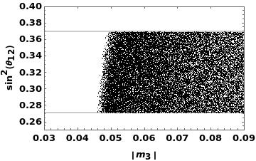
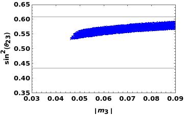
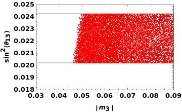
Having included the experimental data, the scattered plots are constructed by using the theoretical formulas given in Eqn.(16) which have to satisfy the experimental values. As a result, the mixing angles as function of the lightest neutrino mass are displayed in Fig. (1). The allowed region of values for the |m30|subscriptsuperscript𝑚03|m^{0}_{3}| is consistent with the previous analytical study.
Refer to caption
Refer to caption
Refer to caption
Figure 1: From left to right: the reactor, solar and atmospheric angles versus the |m30|subscriptsuperscript𝑚03|m^{0}_{3}| lightest neutrino mass. The thick line stands for 3σ3𝜎3\sigma of C. L.

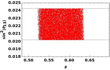
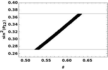
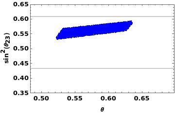
As it was already commented, the θ𝜃\theta parameter is identified with the solar angle in the limit of μτ𝜇𝜏\mu\leftrightarrow\tau exact. Then, the following scattered plots exhibit the region where θ𝜃\theta parameter lies around the experimental value of the solar angle. In fact, this value is close to tribimaximal prediction since the solar angle receives a small correction from ϵitalic-ϵ\epsilon.

Refer to caption
Refer to caption
Refer to caption
Figure 2: From left to right: the reactor, solar and atmospheric angles versus the θ𝜃\theta parameter. The thick line stands for 3σ3𝜎3\sigma of C. L.

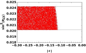
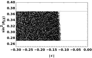
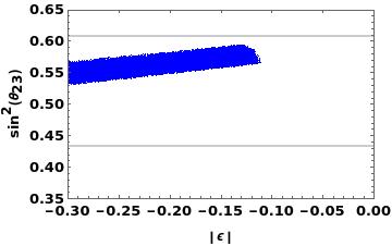
In the previous analytical study, we showed the ϵitalic-ϵ\epsilon parameter must be negative and this may vary in the interval [0,0.3]00.3\left[0,-0.3\right]. The numerical study shows the favored region where the mixing angles are fitted at 3σ3𝜎3\sigma, see Fig. (3). Evidently, the case with |ϵ|=0italic-ϵ0|\epsilon|=0 is excluded due to this stands for the limit of exact μτ𝜇𝜏\mu\leftrightarrow\tau symmetry.

Refer to caption
Refer to caption
Refer to caption
Figure 3: From left to right: the reactor, solar and atmospheric angles versus the |ϵ|italic-ϵ|\epsilon| parameter. The thick line stands for 3σ3𝜎3\sigma of C. L.

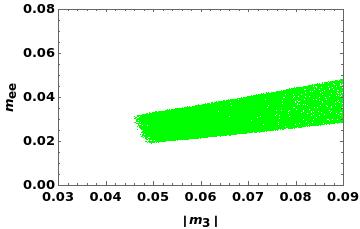
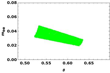
As model prediction, we have calculated numerical the effective Majorana mass of electron neutrino which is defined as follows

|mee|=|i=13mi𝐔ei2|subscript𝑚𝑒𝑒subscriptsuperscript3𝑖1subscript𝑚𝑖subscriptsuperscript𝐔2𝑒𝑖|m_{ee}|=\left|\sum^{3}_{i=1}m_{i}\mathbf{U}^{2}_{ei}\right| (32)

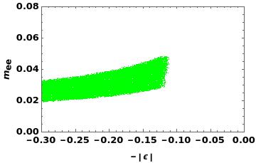
with misubscript𝑚𝑖m_{i} represents the physical neutrino mass and 𝐔eisubscript𝐔𝑒𝑖\mathbf{U}_{ei} PMNS matrix elements. This effective mass has been measured by GERDA phase I[61] and II [62], and the lowest upper bound is |mee|<0.22eVsubscript𝑚𝑒𝑒0.22𝑒𝑉|m_{ee}|<0.22~{}eV.

In our model, CP parities have been used in the neutrino masses. In particular, we utilized m20=|m20|subscriptsuperscript𝑚02subscriptsuperscript𝑚02m^{0}_{2}=-|m^{0}_{2}|, m10=|m10|subscriptsuperscript𝑚01subscriptsuperscript𝑚01m^{0}_{1}=|m^{0}_{1}| and m30=|m30|subscriptsuperscript𝑚03subscriptsuperscript𝑚03m^{0}_{3}=|m^{0}_{3}| since this fit quite well the mixing angles. Consequently, the predicted region for the effective Majorana mass of electron neutrino is shown in the following scattered plots.
Refer to caption
Refer to caption
Refer to caption
Figure 4: The effective Majorana mass of neutrino electron versus the fitted parameters.

III.2 Quark sector

Our numerical study consists in making scattering plots. To do so, we compare our CKM theoretical expression with the standard parametrization one. In particular, we consider the entries (𝐕ui)thsuperscriptsubscript𝐕𝑢𝑖𝑡\left(\mathbf{V}_{ui}\right)^{th} (i=d,s,b𝑖𝑑𝑠𝑏i=d,s,b) and (𝐕cb)thsuperscriptsubscript𝐕𝑐𝑏𝑡\left(\mathbf{V}_{cb}\right)^{th} that depend on the free parameters

|(𝐕ui)th|superscriptsubscript𝐕𝑢𝑖𝑡\displaystyle|\left(\mathbf{V}_{ui}\right)^{th}| =\displaystyle= |(𝐕ui)th(|Eu|,|Ed|,α,β)|;superscriptsubscript𝐕𝑢𝑖𝑡subscript𝐸𝑢subscript𝐸𝑑𝛼𝛽\displaystyle|\left(\mathbf{V}_{ui}\right)^{th}\left(|E_{u}|,|E_{d}|,\alpha,\beta\right)|;
|(𝐕cb)th|superscriptsubscript𝐕𝑐𝑏𝑡\displaystyle|\left(\mathbf{V}_{cb}\right)^{th}| =\displaystyle= |(𝐕ui)th(|Eu|,|Ed|,α,β)|.superscriptsubscript𝐕𝑢𝑖𝑡subscript𝐸𝑢subscript𝐸𝑑𝛼𝛽\displaystyle|\left(\mathbf{V}_{ui}\right)^{th}\left(|E_{u}|,|E_{d}|,\alpha,\beta\right)|. (33)

Therefore, we demand the magnitude of mentioned entries must satisfy the following experimental values [32]

|(𝐕ud)ex|superscriptsubscript𝐕𝑢𝑑𝑒𝑥\displaystyle|\left(\mathbf{V}_{ud}\right)^{ex}| =\displaystyle= 0.97401±0.0001;plus-or-minus0.974010.0001\displaystyle 0.97401\pm 0.0001;
|(𝐕us)ex|superscriptsubscript𝐕𝑢𝑠𝑒𝑥\displaystyle|\left(\mathbf{V}_{us}\right)^{ex}| =\displaystyle= 0.22650±0.0004;plus-or-minus0.226500.0004\displaystyle 0.22650\pm 0.0004;
|(𝐕ub)ex|superscriptsubscript𝐕𝑢𝑏𝑒𝑥\displaystyle|\left(\mathbf{V}_{ub}\right)^{ex}| =\displaystyle= 0.003610.00009+0.00011;subscriptsuperscript0.003610.000110.00009\displaystyle 0.00361^{+0.00011}_{-0.00009};
|(𝐕cb)ex|superscriptsubscript𝐕𝑐𝑏𝑒𝑥\displaystyle|\left(\mathbf{V}_{cb}\right)^{ex}| =\displaystyle= 0.040530.00061+0.00083.subscriptsuperscript0.040530.000830.00061\displaystyle 0.04053^{+0.00083}_{-0.00061}. (34)

In the current study, the physical quark masses are considered as input values. To be more precise, the normalized quark masses (mqi/mq3subscript𝑚subscript𝑞𝑖subscript𝑚subscript𝑞3m_{q_{i}}/m_{q_{3}}) will be used due to their ratios do not change drastically at different energy scales as one can verify directly from [63]. So that, at the top quark mass scale we have [22]

m~usubscript~𝑚𝑢\displaystyle\tilde{m}_{u} =\displaystyle= (1.33±0.73)×105,plus-or-minus1.330.73superscript105\displaystyle(1.33\pm 0.73)\times 10^{-5},
m~csubscript~𝑚𝑐\displaystyle\tilde{m}_{c} =\displaystyle= (3.91±0.42)×103,plus-or-minus3.910.42superscript103\displaystyle(3.91\pm 0.42)\times 10^{-3},
m~dsubscript~𝑚𝑑\displaystyle\tilde{m}_{d} =\displaystyle= (1.49±0.39)×103,plus-or-minus1.490.39superscript103\displaystyle(1.49\pm 0.39)\times 10^{-3},
m~ssubscript~𝑚𝑠\displaystyle\tilde{m}_{s} =\displaystyle= (2.19±0.53)×102.plus-or-minus2.190.53superscript102\displaystyle(2.19\pm 0.53)\times 10^{-2}. (35)

In addition, for simplicity, two dimensionless parameters have been defined yq|Eq|/mq3subscript𝑦𝑞subscript𝐸𝑞subscript𝑚subscript𝑞3y_{q}\equiv|E_{q}|/m_{q_{3}} (q=u,d𝑞𝑢𝑑q=u,d), then we now have the constraint 1>yq>m~q2|mq2|/mq3>m~q11subscript𝑦𝑞subscript~𝑚subscript𝑞2subscript𝑚subscript𝑞2subscript𝑚subscript𝑞3subscript~𝑚subscript𝑞11>y_{q}>\tilde{m}_{q_{2}}\equiv|m_{q_{2}}|/m_{q_{3}}>\tilde{m}_{q_{1}}. Explicitly, for the up and down sector 1>yu>m~c|mc|/mt>m~u1subscript𝑦𝑢subscript~𝑚𝑐subscript𝑚𝑐subscript𝑚𝑡subscript~𝑚𝑢1>y_{u}>\tilde{m}_{c}\equiv|m_{c}|/m_{t}>\tilde{m}_{u} and 1>yd>m~s|ms|/mb>m~d1subscript𝑦𝑑subscript~𝑚𝑠subscript𝑚𝑠subscript𝑚𝑏subscript~𝑚𝑑1>y_{d}>\tilde{m}_{s}\equiv|m_{s}|/m_{b}>\tilde{m}_{d}.

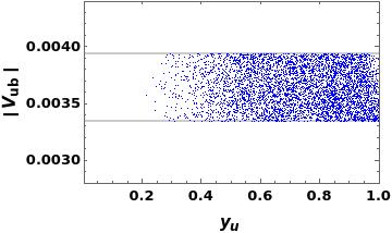
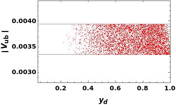
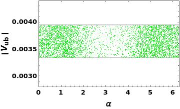
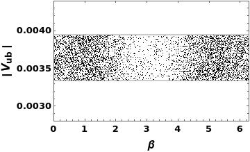
With all the above information, we calculate the allowed regions for the four CKM entries and constrain the free parameter set of values. However, let us show you only the scattered plots for |Vub|subscript𝑉𝑢𝑏|V_{ub}| and |Vcb|subscript𝑉𝑐𝑏|V_{cb}| since that these entries usually are complicated to fit. As we already commented the theoretical expression are required to satisfy the experimental data up to 3σ3𝜎3\sigma. Moreover, the normalized quark masses let vary up to 2σ2𝜎2\sigma and the two CP-violating phases are in the range [0,2π]02𝜋\left[0,2\pi\right]. Then, as one notices, in Figure 5, there is a set of values in which |Vub|subscript𝑉𝑢𝑏|V_{ub}| is fitted with great accuracy.

Refer to caption
Refer to caption
Refer to caption
Refer to caption
Figure 5: |Vub|subscript𝑉𝑢𝑏|V_{ub}| as function of the four free parameters. The thick line stands for 3σ3𝜎3\sigma of C. L.

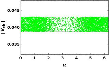
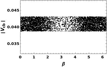
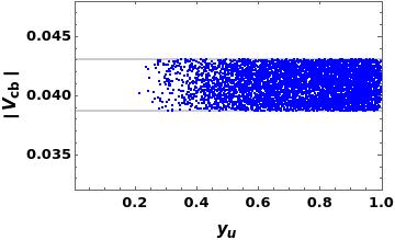
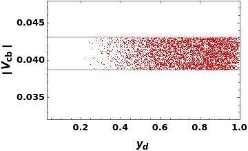
Focusing in the dimensionless parameters yusubscript𝑦𝑢y_{u} and ydsubscript𝑦𝑑y_{d}, the favorable regions lie in [0.5,1)0.51\left[0.5,1\right) approximately. Additionally, there are two regions of values for the CP phases, α𝛼\alpha and β𝛽\beta, where the magnitude of |Vub|subscript𝑉𝑢𝑏|V_{ub}| is accommodated. In the Figure 6, we see |Vcb|subscript𝑉𝑐𝑏|V_{cb}| as function of the four free parameters and these have the same allowed region as the above case.
Refer to caption
Refer to caption
Refer to caption
Refer to caption
Figure 6: |Vcb|subscript𝑉𝑐𝑏|V_{cb}| as function of the four free parameters. The thick line stands for 3σ3𝜎3\sigma of C. L.

To finish this section, we want to comment our naive analysis showed a large region of values for the free parameters where the theoretical CKM entries are in good agreement with the experimental data up to 3σ3𝜎3\sigma. A strict study, as for example an χ2superscript𝜒2\chi^{2} fit, must determine better the space of values however the principal aim of this numerical study was shown the generalized Fritzsch mass textures fit the CKM matrix as it is well known.

IV Summary and conclusions

To sum up, we have built a non-renormalizable model where the fermion mixing is driven by the spontaneous breaking of the 𝐒4𝐙2tensor-productsubscript𝐒4subscript𝐙2\mathbf{S}_{4}\otimes\mathbf{Z}_{2} discrete group. An appropriated alignment of the scalar vev’s allows to break the μτ𝜇𝜏\mu\leftrightarrow\tau symmetry in the effective neutrino mass matrix. Therefore, under a perturbative study, we were able to correct the wrong predictions on the reactor and atmospheric angles, and a set of values for the free parameters was found such that the mixing angles are consistent with the latest neutrino data. Due to the lack of extra symmetries, in the quark sector, a benchmark allows to get consistent mass textures that accommodate the CKM mixing matrix.

We have learned that the flavor symmetries have been useful to eliminate spurious parameters in the Yukawa sector. At the same time, those shape the fermion mass matrices, consequently the mixing pattern can be obtained straightforwardly. Ambitious flavored models have gone beyond of fitting the mixings and prediction on some free parameters (Majorana phases, Dirac CP phase for instance) have been done. In conclusion, despite the μτ𝜇𝜏\mu\leftrightarrow\tau is outdated, in this constrained model, we wanted to show you that a simple soft breaking is enough to correct the mixing angles. Although the model predictions are so limited and the favored inverted hierarchy goes against the data, a soft breaking of μτ𝜇𝜏\mu\leftrightarrow\tau is still alive from theoretical point of view nevertheless the experiments have the verdict.

Acknowledgements

This work was partially supported by Secretaria de Investigación y Posgrado del Instituto Politécnico Nacional under Projects 20221285 and 20220411 and the program PAPIIT IN109321.

Appendix A 𝐒4subscript𝐒4\mathbf{S}_{4} flavour symmetry

𝐒4subscript𝐒4\mathbf{S}_{4} is the group of permutations of four objects and this is the smallest non abelian group having doublet, triplet and singlet irreducible representations [7]. Geometrically, 𝐒4subscript𝐒4\mathbf{S}_{4} is the symmetry of a cube. This discrete group contains five irreducible representations, this is, 𝟏𝟏,𝟏𝟐,𝟐,𝟑𝟏,𝟑𝟐subscript11subscript122subscript31subscript32\mathbf{1_{1},1_{2},2,3_{1},3_{2}} which has the following tensor product rules [7]:

(a1a2)𝟐(b1b2)𝟐tensor-productsubscriptmatrixsubscript𝑎1subscript𝑎22subscriptmatrixsubscript𝑏1subscript𝑏22\displaystyle\begin{pmatrix}a_{1}\\ a_{2}\end{pmatrix}_{\mathbf{2}}\otimes\begin{pmatrix}b_{1}\\ b_{2}\end{pmatrix}_{\mathbf{2}} =(a1b1+a2b2)𝟏1(a1b2+a2b1)𝟏2(a1b2+a2b1a1b1a2b2)𝟐,absentdirect-sumsubscriptsubscript𝑎1subscript𝑏1subscript𝑎2subscript𝑏2subscript11subscriptsubscript𝑎1subscript𝑏2subscript𝑎2subscript𝑏1subscript12subscriptmatrixsubscript𝑎1subscript𝑏2subscript𝑎2subscript𝑏1subscript𝑎1subscript𝑏1subscript𝑎2subscript𝑏22\displaystyle=(a_{1}b_{1}+a_{2}b_{2})_{\mathbf{1}_{1}}\oplus(-a_{1}b_{2}+a_{2}b_{1})_{\mathbf{1}_{2}}\oplus\begin{pmatrix}a_{1}b_{2}+a_{2}b_{1}\\ a_{1}b_{1}-a_{2}b_{2}\end{pmatrix}_{\mathbf{2}\ ,} (36)
(a1a2)𝟐(b1b2b3)𝟑1tensor-productsubscriptmatrixsubscript𝑎1subscript𝑎22subscriptmatrixsubscript𝑏1subscript𝑏2subscript𝑏3subscript31\displaystyle\begin{pmatrix}a_{1}\\ a_{2}\end{pmatrix}_{\mathbf{2}}\otimes\begin{pmatrix}b_{1}\\ b_{2}\\ b_{3}\end{pmatrix}_{\mathbf{3}_{1}} =(a2b112(3a1b2+a2b2)12(3a1b3a2b3))𝟑1(a1b112(3a2b2a1b2)12(3a2b3+a1b3))𝟑2,absentdirect-sumsubscriptmatrixsubscript𝑎2subscript𝑏1123subscript𝑎1subscript𝑏2subscript𝑎2subscript𝑏2123subscript𝑎1subscript𝑏3subscript𝑎2subscript𝑏3subscript31subscriptmatrixsubscript𝑎1subscript𝑏1123subscript𝑎2subscript𝑏2subscript𝑎1subscript𝑏2123subscript𝑎2subscript𝑏3subscript𝑎1subscript𝑏3subscript32\displaystyle=\begin{pmatrix}a_{2}b_{1}\\ -\frac{1}{2}(\sqrt{3}a_{1}b_{2}+a_{2}b_{2})\\ \frac{1}{2}(\sqrt{3}a_{1}b_{3}-a_{2}b_{3})\end{pmatrix}_{\mathbf{3}_{1}}\oplus\begin{pmatrix}a_{1}b_{1}\\ \frac{1}{2}(\sqrt{3}a_{2}b_{2}-a_{1}b_{2})\\ -\frac{1}{2}(\sqrt{3}a_{2}b_{3}+a_{1}b_{3})\end{pmatrix}_{\mathbf{3}_{2}\ ,} (37)
(a1a2)𝟐(b1b2b3)𝟑2tensor-productsubscriptmatrixsubscript𝑎1subscript𝑎22subscriptmatrixsubscript𝑏1subscript𝑏2subscript𝑏3subscript32\displaystyle\begin{pmatrix}a_{1}\\ a_{2}\end{pmatrix}_{\mathbf{2}}\otimes\begin{pmatrix}b_{1}\\ b_{2}\\ b_{3}\end{pmatrix}_{\mathbf{3}_{2}} =(a1b112(3a2b2a1b2)12(3a2b3+a1b3))𝟑1(a2b112(3a1b2+a2b2)12(3a1b3a2b3))𝟑2,absentdirect-sumsubscriptmatrixsubscript𝑎1subscript𝑏1123subscript𝑎2subscript𝑏2subscript𝑎1subscript𝑏2123subscript𝑎2subscript𝑏3subscript𝑎1subscript𝑏3subscript31subscriptmatrixsubscript𝑎2subscript𝑏1123subscript𝑎1subscript𝑏2subscript𝑎2subscript𝑏2123subscript𝑎1subscript𝑏3subscript𝑎2subscript𝑏3subscript32\displaystyle=\begin{pmatrix}a_{1}b_{1}\\ \frac{1}{2}(\sqrt{3}a_{2}b_{2}-a_{1}b_{2})\\ -\frac{1}{2}(\sqrt{3}a_{2}b_{3}+a_{1}b_{3})\end{pmatrix}_{\mathbf{3}_{1}}\oplus\begin{pmatrix}a_{2}b_{1}\\ -\frac{1}{2}(\sqrt{3}a_{1}b_{2}+a_{2}b_{2})\\ \frac{1}{2}(\sqrt{3}a_{1}b_{3}-a_{2}b_{3})\end{pmatrix}_{\mathbf{3}_{2}\ ,} (38)
(a1a2a3)𝟑1(b1b2b3)𝟑1tensor-productsubscriptmatrixsubscript𝑎1subscript𝑎2subscript𝑎3subscript31subscriptmatrixsubscript𝑏1subscript𝑏2subscript𝑏3subscript31\displaystyle\begin{pmatrix}a_{1}\\ a_{2}\\ a_{3}\end{pmatrix}_{\mathbf{3}_{1}}\otimes\begin{pmatrix}b_{1}\\ b_{2}\\ b_{3}\end{pmatrix}_{\mathbf{3}_{1}} =(a1b1+a2b2+a3b3)𝟏1(12(a2b2a3b3)16(2a1b1+a2b2+a3b3))𝟐absentdirect-sumsubscriptsubscript𝑎1subscript𝑏1subscript𝑎2subscript𝑏2subscript𝑎3subscript𝑏3subscript11subscriptmatrix12subscript𝑎2subscript𝑏2subscript𝑎3subscript𝑏3162subscript𝑎1subscript𝑏1subscript𝑎2subscript𝑏2subscript𝑎3subscript𝑏32\displaystyle=(a_{1}b_{1}+a_{2}b_{2}+a_{3}b_{3})_{\mathbf{1}_{1}}\oplus\begin{pmatrix}\frac{1}{\sqrt{2}}(a_{2}b_{2}-a_{3}b_{3})\\ \frac{1}{\sqrt{6}}(-2a_{1}b_{1}+a_{2}b_{2}+a_{3}b_{3})\end{pmatrix}_{\mathbf{2}}
(a2b3+a3b2a1b3+a3b1a1b2+a2b1)𝟑1(a3b2a2b3a1b3a3b1a2b1a1b2)𝟑2,direct-sumdirect-sumsubscriptmatrixsubscript𝑎2subscript𝑏3subscript𝑎3subscript𝑏2subscript𝑎1subscript𝑏3subscript𝑎3subscript𝑏1subscript𝑎1subscript𝑏2subscript𝑎2subscript𝑏1subscript31subscriptmatrixsubscript𝑎3subscript𝑏2subscript𝑎2subscript𝑏3subscript𝑎1subscript𝑏3subscript𝑎3subscript𝑏1subscript𝑎2subscript𝑏1subscript𝑎1subscript𝑏2subscript32\displaystyle\ \oplus\begin{pmatrix}a_{2}b_{3}+a_{3}b_{2}\\ a_{1}b_{3}+a_{3}b_{1}\\ a_{1}b_{2}+a_{2}b_{1}\end{pmatrix}_{\mathbf{3}_{1}}\oplus\begin{pmatrix}a_{3}b_{2}-a_{2}b_{3}\\ a_{1}b_{3}-a_{3}b_{1}\\ a_{2}b_{1}-a_{1}b_{2}\end{pmatrix}_{\mathbf{3}_{2}\ ,} (39)
(a1a2a3)𝟑2(b1b2b3)𝟑2tensor-productsubscriptmatrixsubscript𝑎1subscript𝑎2subscript𝑎3subscript32subscriptmatrixsubscript𝑏1subscript𝑏2subscript𝑏3subscript32\displaystyle\begin{pmatrix}a_{1}\\ a_{2}\\ a_{3}\end{pmatrix}_{\mathbf{3}_{2}}\otimes\begin{pmatrix}b_{1}\\ b_{2}\\ b_{3}\end{pmatrix}_{\mathbf{3}_{2}} =(a1b1+a2b2+a3b3)𝟏1(12(a2b2a3b3)16(2a1b1+a2b2+a3b3))𝟐absentdirect-sumsubscriptsubscript𝑎1subscript𝑏1subscript𝑎2subscript𝑏2subscript𝑎3subscript𝑏3subscript11subscriptmatrix12subscript𝑎2subscript𝑏2subscript𝑎3subscript𝑏3162subscript𝑎1subscript𝑏1subscript𝑎2subscript𝑏2subscript𝑎3subscript𝑏32\displaystyle=(a_{1}b_{1}+a_{2}b_{2}+a_{3}b_{3})_{\mathbf{1}_{1}}\oplus\begin{pmatrix}\frac{1}{\sqrt{2}}(a_{2}b_{2}-a_{3}b_{3})\\ \frac{1}{\sqrt{6}}(-2a_{1}b_{1}+a_{2}b_{2}+a_{3}b_{3})\end{pmatrix}_{\mathbf{2}}
(a2b3+a3b2a1b3+a3b1a1b2+a2b1)𝟑1(a3b2a2b3a1b3a3b1a2b1a1b2)𝟑2,direct-sumdirect-sumsubscriptmatrixsubscript𝑎2subscript𝑏3subscript𝑎3subscript𝑏2subscript𝑎1subscript𝑏3subscript𝑎3subscript𝑏1subscript𝑎1subscript𝑏2subscript𝑎2subscript𝑏1subscript31subscriptmatrixsubscript𝑎3subscript𝑏2subscript𝑎2subscript𝑏3subscript𝑎1subscript𝑏3subscript𝑎3subscript𝑏1subscript𝑎2subscript𝑏1subscript𝑎1subscript𝑏2subscript32\displaystyle\ \oplus\begin{pmatrix}a_{2}b_{3}+a_{3}b_{2}\\ a_{1}b_{3}+a_{3}b_{1}\\ a_{1}b_{2}+a_{2}b_{1}\end{pmatrix}_{\mathbf{3}_{1}}\oplus\begin{pmatrix}a_{3}b_{2}-a_{2}b_{3}\\ a_{1}b_{3}-a_{3}b_{1}\\ a_{2}b_{1}-a_{1}b_{2}\end{pmatrix}_{\mathbf{3}_{2}\ ,} (40)
(a1a2a3)𝟑1(b1b2b3)𝟑2tensor-productsubscriptmatrixsubscript𝑎1subscript𝑎2subscript𝑎3subscript31subscriptmatrixsubscript𝑏1subscript𝑏2subscript𝑏3subscript32\displaystyle\begin{pmatrix}a_{1}\\ a_{2}\\ a_{3}\end{pmatrix}_{\mathbf{3}_{1}}\otimes\begin{pmatrix}b_{1}\\ b_{2}\\ b_{3}\end{pmatrix}_{\mathbf{3}_{2}} =(a1b1+a2b2+a3b3)𝟏2(16(2a1b1a2b2a3b3)12(a2b2a3b3))𝟐absentdirect-sumsubscriptsubscript𝑎1subscript𝑏1subscript𝑎2subscript𝑏2subscript𝑎3subscript𝑏3subscript12subscriptmatrix162subscript𝑎1subscript𝑏1subscript𝑎2subscript𝑏2subscript𝑎3subscript𝑏312subscript𝑎2subscript𝑏2subscript𝑎3subscript𝑏32\displaystyle=(a_{1}b_{1}+a_{2}b_{2}+a_{3}b_{3})_{\mathbf{1}_{2}}\oplus\begin{pmatrix}\frac{1}{\sqrt{6}}(2a_{1}b_{1}-a_{2}b_{2}-a_{3}b_{3})\\ \frac{1}{\sqrt{2}}(a_{2}b_{2}-a_{3}b_{3})\end{pmatrix}_{\mathbf{2}}
(a3b2a2b3a1b3a3b1a2b1a1b2)𝟑1(a2b3+a3b2a1b3+a3b1a1b2+a2b1)𝟑2.direct-sumdirect-sumsubscriptmatrixsubscript𝑎3subscript𝑏2subscript𝑎2subscript𝑏3subscript𝑎1subscript𝑏3subscript𝑎3subscript𝑏1subscript𝑎2subscript𝑏1subscript𝑎1subscript𝑏2subscript31subscriptmatrixsubscript𝑎2subscript𝑏3subscript𝑎3subscript𝑏2subscript𝑎1subscript𝑏3subscript𝑎3subscript𝑏1subscript𝑎1subscript𝑏2subscript𝑎2subscript𝑏1subscript32\displaystyle\ \oplus\begin{pmatrix}a_{3}b_{2}-a_{2}b_{3}\\ a_{1}b_{3}-a_{3}b_{1}\\ a_{2}b_{1}-a_{1}b_{2}\end{pmatrix}_{\mathbf{3}_{1}}\oplus\begin{pmatrix}a_{2}b_{3}+a_{3}b_{2}\\ a_{1}b_{3}+a_{3}b_{1}\\ a_{1}b_{2}+a_{2}b_{1}\end{pmatrix}_{\mathbf{3}_{2}\ .} (41)

In this section, we remark an interesting feature between the 𝐒3subscript𝐒3\mathbf{S}_{3} [7] and 𝐒4subscript𝐒4\mathbf{S}_{4} non-abelian groups. As it is well known, these are different, the former one has three irreducible representations namely two singlets, 𝟏𝟏subscript11\mathbf{1_{1}} and 𝟏𝟐subscript12\mathbf{1_{2}}, and one doublet 𝟐2\mathbf{2}. This group is smaller than 𝐒4subscript𝐒4\mathbf{S}_{4} as one can see in  [7]. In addition, each representation of 𝐒4subscript𝐒4\mathbf{S}_{4} can be decomposed in representation of 𝐒3subscript𝐒3\mathbf{S}_{3} as follows: 𝟏1𝟏1subscript11subscript11\mathbf{1}_{1}\rightarrow\mathbf{1}_{1}, 𝟏2𝟏2subscript12subscript12\mathbf{1}_{2}\rightarrow\mathbf{1}_{2}, 𝟐𝟐22\mathbf{2}\rightarrow\mathbf{2}, 𝟑1𝟏1𝟐subscript31direct-sumsubscript112\mathbf{3}_{1}\rightarrow\mathbf{1}_{1}\oplus\mathbf{2} and 𝟑2𝟏2𝟐subscript32direct-sumsubscript122\mathbf{3}_{2}\rightarrow\mathbf{1}_{2}\oplus\mathbf{2}.

Appendix B Symmetry μτ𝜇𝜏\mu\leftrightarrow\tau

In the basis where the charged lepton mass matrix is diagonal, the effective neutrino mass term is given by

=ν¯L(𝐌ν)(νL)C+h.c,formulae-sequencesubscript¯𝜈𝐿subscriptsubscript𝐌𝜈superscriptsuperscriptsubscript𝜈superscript𝐿𝐶𝑐\mathcal{L}=\bar{\nu}_{\ell L}(\mathbf{M}_{\nu})_{\ell\ell^{\prime}}(\nu_{\ell^{\prime}L})^{C}+h.c, (42)

where ,=e,μ,τformulae-sequencesuperscript𝑒𝜇𝜏\ell,\ell^{\prime}=e,\mu,\tau. If the neutrino mass matrix is invariant under the interchange label μτ𝜇𝜏\mu\leftrightarrow\tau, one would have

𝐌ν=(meemeμmeμmeμmμμmμτmeμmμτmμμ).subscript𝐌𝜈matrixsubscript𝑚𝑒𝑒subscript𝑚𝑒𝜇subscript𝑚𝑒𝜇subscript𝑚𝑒𝜇subscript𝑚𝜇𝜇subscript𝑚𝜇𝜏subscript𝑚𝑒𝜇subscript𝑚𝜇𝜏subscript𝑚𝜇𝜇\mathbf{M}_{\nu}=\begin{pmatrix}m_{ee}&m_{e\mu}&m_{e\mu}\\ m_{e\mu}&m_{\mu\mu}&m_{\mu\tau}\\ m_{e\mu}&m_{\mu\tau}&m_{\mu\mu}\end{pmatrix}. (43)

As one can notice, in the previous mass matrix the entries 121212 (222222) and 131313 (333333) are equals, then that matrix possesses the μτ𝜇𝜏\mu\leftrightarrow\tau symmetry [64, 65, 66, 67, 68] and its prediction on the mixing angles are obtained as follows. In the mentioned basis, the neutrino mass matrix is diagonalized by 𝐔νsubscript𝐔𝜈\mathbf{U}_{\nu}, this means, 𝐔ν𝐌ν𝐔ν=𝐌^subscriptsuperscript𝐔𝜈subscript𝐌𝜈subscriptsuperscript𝐔𝜈^𝐌\mathbf{U}^{\dagger}_{\nu}\mathbf{M}_{\nu}\mathbf{U}^{\ast}_{\nu}=\hat{\mathbf{M}} where the latter matrix stands for the neutrino masses, 𝐌^=Diag.(m1,m2,m3)formulae-sequence^𝐌Diagsubscript𝑚1subscript𝑚2subscript𝑚3\hat{\mathbf{M}}=\textrm{Diag}.(m_{1},m_{2},m_{3}), which can be complex.

As it is well known, 𝐔ν=𝐔π/4𝐔θsubscript𝐔𝜈subscript𝐔𝜋4subscript𝐔𝜃\mathbf{U}_{\nu}=\mathbf{U}_{\pi/4}\mathbf{U}_{\theta} so that 𝐔ν𝐌ν𝐔ν=𝐔θ𝐦ν𝐔θsubscriptsuperscript𝐔𝜈subscript𝐌𝜈subscriptsuperscript𝐔𝜈subscriptsuperscript𝐔𝜃subscript𝐦𝜈subscriptsuperscript𝐔𝜃\mathbf{U}^{\dagger}_{\nu}\mathbf{M}_{\nu}\mathbf{U}^{\ast}_{\nu}=\mathbf{U}^{\dagger}_{\theta}\mathbf{m}_{\nu}\mathbf{U}^{\ast}_{\theta} where

𝐦ν=(mee2meμ02meμmμμ+mμτ000mμμmμτ),𝐔π/4=(1000121201212).formulae-sequencesubscript𝐦𝜈matrixsubscript𝑚𝑒𝑒2subscript𝑚𝑒𝜇02subscript𝑚𝑒𝜇subscript𝑚𝜇𝜇subscript𝑚𝜇𝜏000subscript𝑚𝜇𝜇subscript𝑚𝜇𝜏subscript𝐔𝜋4matrix1000121201212\mathbf{m}_{\nu}=\begin{pmatrix}m_{ee}&\sqrt{2}m_{e\mu}&0\\ \sqrt{2}m_{e\mu}&m_{\mu\mu}+m_{\mu\tau}&0\\ 0&0&m_{\mu\mu}-m_{\mu\tau}\end{pmatrix},\qquad\mathbf{U}_{\pi/4}=\begin{pmatrix}1&0&0\\ 0&\frac{1}{\sqrt{2}}&-\frac{1}{\sqrt{2}}\\ 0&\frac{1}{\sqrt{2}}&\frac{1}{\sqrt{2}}\end{pmatrix}. (44)

In addition, 𝐦νsubscript𝐦𝜈\mathbf{m}_{\nu} is diagonalized by 𝐔θνsubscript𝐔subscript𝜃𝜈\mathbf{U}_{\theta_{\nu}} whose form is given as

𝐔θ=(cosθsinθ0sinθcosθ0001),subscript𝐔𝜃matrix𝜃𝜃0𝜃𝜃0001\mathbf{U}_{\theta}=\begin{pmatrix}\cos{\theta}&\sin{\theta}&0\\ -\sin{\theta}&\cos{\theta}&0\\ 0&0&1\end{pmatrix}, (45)

and one condition should be satisfied

tan2θ=8meμmμμ+mμτmee.2𝜃8subscript𝑚𝑒𝜇subscript𝑚𝜇𝜇subscript𝑚𝜇𝜏subscript𝑚𝑒𝑒\tan{2\theta}=\frac{\sqrt{8}m_{e\mu}}{m_{\mu\mu}+m_{\mu\tau}-m_{ee}}. (46)

Therefore, one can write the full matrix

𝐔ν=(cosθsinθ0sinθ2cosθ212sinθ2cosθ212).subscript𝐔𝜈matrix𝜃𝜃0𝜃2𝜃212𝜃2𝜃212\mathbf{U}_{\nu}=\begin{pmatrix}\cos{\theta}&\sin{\theta}&0\\ -\frac{\sin{\theta}}{\sqrt{2}}&\frac{\cos{\theta}}{\sqrt{2}}&-\frac{1}{\sqrt{2}}\\ -\frac{\sin{\theta}}{\sqrt{2}}&\frac{\cos{\theta}}{\sqrt{2}}&\frac{1}{\sqrt{2}}\end{pmatrix}. (47)

Comparing the above mixing matrix with the standard parametrization of the PMNS matrix, one gets the reactor and atmospheric angles are θ13=0subscript𝜃130\theta_{13}=0 and θ23=π/4subscript𝜃23𝜋4\theta_{23}=\pi/4, respectively. Speaking about the solar angle, this is free parameter and can be identified by θ12=θsubscript𝜃12𝜃\theta_{12}=\theta.

At the same time, the matrix elements can be written in terms of the physical neutrino mass as follows

meesubscript𝑚𝑒𝑒\displaystyle m_{ee} =\displaystyle= m1cos2θ+m2sin2θ,subscript𝑚1superscript2𝜃subscript𝑚2superscript2𝜃\displaystyle m_{1}\cos^{2}{\theta}+m_{2}\sin^{2}{\theta},
meμsubscript𝑚𝑒𝜇\displaystyle m_{e\mu} =\displaystyle= sin2θ8(m2m1),2𝜃8subscript𝑚2subscript𝑚1\displaystyle\frac{\sin{2\theta}}{\sqrt{8}}\left(m_{2}-m_{1}\right),
mμτsubscript𝑚𝜇𝜏\displaystyle m_{\mu\tau} =\displaystyle= 12(m1sin2θ+m2cos2θ+m3),12subscript𝑚1superscript2𝜃subscript𝑚2superscript2𝜃subscript𝑚3\displaystyle\frac{1}{2}\left(m_{1}\sin^{2}{\theta}+m_{2}\cos^{2}{\theta}+m_{3}\right),
mμμsubscript𝑚𝜇𝜇\displaystyle m_{\mu\mu} =\displaystyle= 12(m1sin2θ+m2cos2θm3).12subscript𝑚1superscript2𝜃subscript𝑚2superscript2𝜃subscript𝑚3\displaystyle\frac{1}{2}\left(m_{1}\sin^{2}{\theta}+m_{2}\cos^{2}{\theta}-m_{3}\right). (48)

Appendix C Perturbative study to obtain 𝐔νϵsubscriptsuperscript𝐔italic-ϵ𝜈\mathbf{U}^{\epsilon}_{\nu}

To start with, we have to remember the stationary perturbation theory from our lectures on quantum mechanics [69]. This method is applied to a system whose Hamiltonian is given by H=H0+W𝐻subscript𝐻0𝑊H=H_{0}+W where the eigenstates (ϕn0subscriptsuperscriptitalic-ϕ0𝑛\phi^{0}_{n}) and eigenvalues (En0subscriptsuperscript𝐸0𝑛E^{0}_{n}) of H0subscript𝐻0H_{0} are known, also W𝑊W (known as a perturbation) is smaller than H0subscript𝐻0H_{0}, besides that, H0subscript𝐻0H_{0} and W𝑊W are time independent. With W=λW~𝑊𝜆~𝑊W=\lambda~{}\tilde{W} and λ1much-less-than𝜆1\lambda\ll 1, at first order in the λ𝜆\lambda perturbative parameter, one can perform the correction to the eigenstates and eigenvalues of H(λ)𝐻𝜆H(\lambda) ( H(λ)|Φn(λ)=En(λ)|Φn(λ)𝐻𝜆ketsubscriptΦ𝑛𝜆subscript𝐸𝑛𝜆ketsubscriptΦ𝑛𝜆H(\lambda)|\Phi_{n}(\lambda)\rangle=E_{n}(\lambda)|\Phi_{n}(\lambda)\rangle) which are given respectively by

|Φn(λ)=|ϕn0+knϕk0|W|ϕn0En0Ek0|ϕk0,En(λ)=En0+ϕn0|W|ϕn0.formulae-sequenceketsubscriptΦ𝑛𝜆ketsubscriptsuperscriptitalic-ϕ0𝑛subscript𝑘𝑛quantum-operator-productsubscriptsuperscriptitalic-ϕ0𝑘𝑊subscriptsuperscriptitalic-ϕ0𝑛subscriptsuperscript𝐸0𝑛subscriptsuperscript𝐸0𝑘ketsubscriptsuperscriptitalic-ϕ0𝑘subscript𝐸𝑛𝜆subscriptsuperscript𝐸0𝑛quantum-operator-productsubscriptsuperscriptitalic-ϕ0𝑛𝑊subscriptsuperscriptitalic-ϕ0𝑛|\Phi_{n}(\lambda)\rangle=|\phi^{0}_{n}\rangle+\displaystyle\sum_{k\neq n}\frac{\langle\phi^{0}_{k}|W|\phi^{0}_{n}\rangle}{E^{0}_{n}-E^{0}_{k}}|\phi^{0}_{k}\rangle,\qquad E_{n}(\lambda)=E^{0}_{n}+\langle\phi^{0}_{n}|W|\phi^{0}_{n}\rangle. (49)

Then, we adapt the above results to diagonalization problem given in the neutrino sector. As it was shown, νsubscript𝜈\mathbf{\mathcal{M}}_{\nu} is diagonalized by the 𝐔νsubscript𝐔𝜈\mathbf{U}_{\nu} matrix such that 𝐌^ν=Diag.(m1,m2,m3)=𝐔νν𝐔νsubscript^𝐌𝜈Diag.subscript𝑚1subscript𝑚2subscript𝑚3subscriptsuperscript𝐔𝜈subscript𝜈subscriptsuperscript𝐔𝜈\hat{\mathbf{M}}_{\nu}=\textrm{Diag.}\left(m_{1},m_{2},m_{3}\right)=\mathbf{U}^{\dagger}_{\nu}\mathbf{\mathcal{M}}_{\nu}\mathbf{U}^{\ast}_{\nu} with 𝐔ν=𝐒23𝐮νsubscript𝐔𝜈subscript𝐒23subscript𝐮𝜈\mathbf{U}_{\nu}=\mathbf{S}_{23}\mathbf{u}_{\nu}, then 𝐌^ν=𝐮ν𝐦ν𝐮νsubscript^𝐌𝜈subscriptsuperscript𝐮𝜈subscript𝐦𝜈subscriptsuperscript𝐮𝜈\hat{\mathbf{M}}_{\nu}=\mathbf{u}^{\dagger}_{\nu}\mathbf{m}_{\nu}\mathbf{u}^{\ast}_{\nu}. 𝐦νsubscript𝐦𝜈\mathbf{m}_{\nu} can be written as

𝐦ν=(meemeμmeμmeμmμμmμτmeμmμτmμμ)𝐦ν0+(00000000mμμϵ)𝐦νϵ,subscript𝐦𝜈superscriptmatrixsubscript𝑚𝑒𝑒subscript𝑚𝑒𝜇subscript𝑚𝑒𝜇subscript𝑚𝑒𝜇subscript𝑚𝜇𝜇subscript𝑚𝜇𝜏subscript𝑚𝑒𝜇subscript𝑚𝜇𝜏subscript𝑚𝜇𝜇subscriptsuperscript𝐦0𝜈superscriptmatrix00000000subscript𝑚𝜇𝜇italic-ϵsubscriptsuperscript𝐦italic-ϵ𝜈\mathbf{m}_{\nu}=\overbrace{\begin{pmatrix}m_{ee}&m_{e\mu}&m_{e\mu}\\ m_{e\mu}&m_{\mu\mu}&m_{\mu\tau}\\ m_{e\mu}&m_{\mu\tau}&m_{\mu\mu}\end{pmatrix}}^{\mathbf{m}^{0}_{\nu}}+\overbrace{\begin{pmatrix}0&0&0\\ 0&0&0\\ 0&0&m_{\mu\mu}\epsilon\end{pmatrix}}^{\mathbf{m}^{\epsilon}_{\nu}}, (50)

where the former matrix possesses exact μτ𝜇𝜏\mu\leftrightarrow\tau symmetry and it is broken in the latter one where the dimensionless parameter ϵ(mττmμμ)/mμμitalic-ϵsubscript𝑚𝜏𝜏subscript𝑚𝜇𝜇subscript𝑚𝜇𝜇\epsilon\equiv\left(m_{\tau\tau}-m_{\mu\mu}\right)/m_{\mu\mu} has been defined and this quantify the breaking. In addition, this parameter will be treated as a perturbation, thus, a pertubative study at first order in ϵitalic-ϵ\epsilon will be carried out. It was shown in the above Appendix, 𝐦ν0subscriptsuperscript𝐦0𝜈\mathbf{m}^{0}_{\nu} is diagonalized by 𝐔ν0subscriptsuperscript𝐔0𝜈\mathbf{U}^{0}_{\nu}, then, 𝐌^ν=𝐮ν𝐦ν𝐮νsubscript^𝐌𝜈subscriptsuperscript𝐮𝜈subscript𝐦𝜈subscriptsuperscript𝐮𝜈\hat{\mathbf{M}}_{\nu}=\mathbf{u}^{\dagger}_{\nu}\mathbf{m}_{\nu}\mathbf{u}^{\ast}_{\nu} with 𝐮ν𝐔ν0𝐔νϵsubscript𝐮𝜈subscriptsuperscript𝐔0𝜈subscriptsuperscript𝐔italic-ϵ𝜈\mathbf{u}_{\nu}\approx\mathbf{U}^{0}_{\nu}\mathbf{U}^{\epsilon}_{\nu} implies

𝐌^ν=𝐔νϵ[𝐔ν0𝐦ν0𝐔ν0+𝐔ν0𝐦νϵ𝐔ν0]𝐔νϵ,with𝐔ν0𝐦ν0𝐔ν0=Diag.(m10,m20,m30).formulae-sequencesubscript^𝐌𝜈subscriptsuperscript𝐔italic-ϵ𝜈delimited-[]subscriptsuperscript𝐔0𝜈subscriptsuperscript𝐦0𝜈subscriptsuperscript𝐔0𝜈subscriptsuperscript𝐔0𝜈subscriptsuperscript𝐦italic-ϵ𝜈subscriptsuperscript𝐔0𝜈subscriptsuperscript𝐔italic-ϵ𝜈withsubscriptsuperscript𝐔0𝜈subscriptsuperscript𝐦0𝜈subscriptsuperscript𝐔0𝜈Diag.subscriptsuperscript𝑚01subscriptsuperscript𝑚02subscriptsuperscript𝑚03\hat{\mathbf{M}}_{\nu}=\mathbf{U}^{\epsilon\dagger}_{\nu}\left[\mathbf{U}^{0\dagger}_{\nu}\mathbf{m}^{0}_{\nu}\mathbf{U}^{0\ast}_{\nu}+\mathbf{U}^{0\dagger}_{\nu}\mathbf{m}^{\epsilon}_{\nu}\mathbf{U}^{0\ast}_{\nu}\right]\mathbf{U}^{\epsilon\ast}_{\nu},\quad\textrm{with}\quad\mathbf{U}^{0\dagger}_{\nu}\mathbf{m}^{0}_{\nu}\mathbf{U}^{0\ast}_{\nu}=\textrm{Diag.}\left(m^{0}_{1},m^{0}_{2},m^{0}_{3}\right). (51)

In addition,

𝐔ν0𝐦νϵ𝐔ν0m~νϵ=ϵmμμ02(sin2θsin2θ2sinθsin2θ2cos2θcosθsinθcosθ1),mμμ0=12(m10sin2θ+m20cos2θm30).formulae-sequencesuperscriptsubscriptsuperscript𝐔0𝜈subscriptsuperscript𝐦italic-ϵ𝜈subscriptsuperscript𝐔0𝜈subscriptsuperscript~𝑚italic-ϵ𝜈italic-ϵsubscriptsuperscript𝑚0𝜇𝜇2matrixsuperscript2𝜃2𝜃2𝜃2𝜃2superscript2𝜃𝜃𝜃𝜃1subscriptsuperscript𝑚0𝜇𝜇12subscriptsuperscript𝑚01superscript2𝜃subscriptsuperscript𝑚02superscript2𝜃subscriptsuperscript𝑚03\overbrace{\mathbf{U}^{0\dagger}_{\nu}\mathbf{m}^{\epsilon}_{\nu}\mathbf{U}^{0\ast}_{\nu}}^{\tilde{m}^{\epsilon}_{\nu}}=\frac{\epsilon~{}m^{0}_{\mu\mu}}{2}\begin{pmatrix}\sin^{2}{\theta}&-\frac{\sin{2\theta}}{2}&-\sin{\theta}\\ -\frac{\sin{2\theta}}{2}&\cos^{2}{\theta}&\cos{\theta}\\ -\sin{\theta}&\cos{\theta}&1\end{pmatrix},\qquad m^{0}_{\mu\mu}=\frac{1}{2}\left(m^{0}_{1}\sin^{2}{\theta}+m^{0}_{2}\cos^{2}{\theta}-m^{0}_{3}\right). (52)

In here, we make contact with the perturbation theory, instead of having a Hamiltonian, we have 𝐦ν=𝐦ν0+𝐦νϵsubscript𝐦𝜈subscriptsuperscript𝐦0𝜈subscriptsuperscript𝐦italic-ϵ𝜈\mathbf{m}_{\nu}=\mathbf{m}^{0}_{\nu}+\mathbf{m}^{\epsilon}_{\nu} where the eigenstates (νi0subscriptsuperscript𝜈0𝑖\nu^{0}_{i}) and eigenvalues (mi0subscriptsuperscript𝑚0𝑖m^{0}_{i}) of 𝐦ν0subscriptsuperscript𝐦0𝜈\mathbf{m}^{0}_{\nu} are well known. In consequence, 𝐔νϵsubscriptsuperscript𝐔italic-ϵ𝜈\mathbf{U}^{\epsilon}_{\nu} is built by means the adapted eigenvector, this is, 𝐔νϵ=(|Φ1(ϵ),|Φ2(ϵ),|Φ3(ϵ))subscriptsuperscript𝐔italic-ϵ𝜈ketsubscriptΦ1italic-ϵketsubscriptΦ2italic-ϵketsubscriptΦ3italic-ϵ\mathbf{U}^{\epsilon}_{\nu}=\left(|\Phi_{1}(\epsilon)\rangle,|\Phi_{2}(\epsilon)\rangle,|\Phi_{3}(\epsilon)\rangle\right) where

|Φn(ϵ)=|νn0+kn3νk0|m~νϵ|νn0mn0mk0|νk0ketsubscriptΦ𝑛italic-ϵketsubscriptsuperscript𝜈0𝑛subscriptsuperscript3𝑘𝑛quantum-operator-productsubscriptsuperscript𝜈0𝑘subscriptsuperscript~𝑚italic-ϵ𝜈subscriptsuperscript𝜈0𝑛subscriptsuperscript𝑚0𝑛subscriptsuperscript𝑚0𝑘ketsubscriptsuperscript𝜈0𝑘|\Phi_{n}(\epsilon)\rangle=|\nu^{0}_{n}\rangle+\displaystyle\sum^{3}_{k\neq n}\frac{\langle\nu^{0}_{k}|\tilde{m}^{\epsilon}_{\nu}|\nu^{0}_{n}\rangle}{m^{0}_{n}-m^{0}_{k}}|\nu^{0}_{k}\rangle (53)

where n=1,2,3𝑛123n=1,2,3. In order to apply correctly the formula, we have to observe that matrix 𝐦νϵsubscriptsuperscript𝐦italic-ϵ𝜈\mathbf{m}^{\epsilon}_{\nu} has been rotated by 𝐔ν0subscriptsuperscript𝐔0𝜈\mathbf{U}^{0}_{\nu} so that the new perturbative matrix is denoted by m~νϵsubscriptsuperscript~𝑚italic-ϵ𝜈\tilde{m}^{\epsilon}_{\nu}. Additionally, each eigenvector |Φn(ϵ)ketsubscriptΦ𝑛italic-ϵ|\Phi_{n}(\epsilon)\rangle must be normalized. Finally, one gets

𝐔νϵ(N1mμμ0m20m10sin2θ4ϵN2mμμ0m10m30sinθ2ϵN3mμμ0m20m10sin2θ4ϵN1N2mμμ0m20m30cosθ2ϵN3mμμ0m10m30sinθ2ϵN1mμμ0m20m30cosθ2ϵN2N3),subscriptsuperscript𝐔italic-ϵ𝜈matrixsubscript𝑁1subscriptsuperscript𝑚0𝜇𝜇subscriptsuperscript𝑚02subscriptsuperscript𝑚012𝜃4italic-ϵsubscript𝑁2subscriptsuperscript𝑚0𝜇𝜇subscriptsuperscript𝑚01subscriptsuperscript𝑚03𝜃2italic-ϵsubscript𝑁3subscriptsuperscript𝑚0𝜇𝜇subscriptsuperscript𝑚02subscriptsuperscript𝑚012𝜃4italic-ϵsubscript𝑁1subscript𝑁2subscriptsuperscript𝑚0𝜇𝜇subscriptsuperscript𝑚02subscriptsuperscript𝑚03𝜃2italic-ϵsubscript𝑁3subscriptsuperscript𝑚0𝜇𝜇subscriptsuperscript𝑚01subscriptsuperscript𝑚03𝜃2italic-ϵsubscript𝑁1subscriptsuperscript𝑚0𝜇𝜇subscriptsuperscript𝑚02subscriptsuperscript𝑚03𝜃2italic-ϵsubscript𝑁2subscript𝑁3\mathbf{U}^{\epsilon}_{\nu}\approx\begin{pmatrix}N_{1}&-\frac{m^{0}_{\mu\mu}}{m^{0}_{2}-m^{0}_{1}}\frac{\sin{2\theta}}{4}\epsilon N_{2}&\frac{m^{0}_{\mu\mu}}{m^{0}_{1}-m^{0}_{3}}\frac{\sin{\theta}}{2}\epsilon N_{3}\\ \frac{m^{0}_{\mu\mu}}{m^{0}_{2}-m^{0}_{1}}\frac{\sin{2\theta}}{4}\epsilon N_{1}&N_{2}&-\frac{m^{0}_{\mu\mu}}{m^{0}_{2}-m^{0}_{3}}\frac{\cos{\theta}}{2}\epsilon N_{3}\\ -\frac{m^{0}_{\mu\mu}}{m^{0}_{1}-m^{0}_{3}}\frac{\sin{\theta}}{2}\epsilon N_{1}&\frac{m^{0}_{\mu\mu}}{m^{0}_{2}-m^{0}_{3}}\frac{\cos{\theta}}{2}\epsilon N_{2}&N_{3}\end{pmatrix}, (54)

where the normalization factors are written as

N1subscript𝑁1\displaystyle N_{1} =\displaystyle= [1+|ϵ|2sin2θ4(|mμμ0m10m30|2+cos2θ|mμμ0m20m10|2)]1/2,superscriptdelimited-[]1superscriptitalic-ϵ2superscript2𝜃4superscriptsubscriptsuperscript𝑚0𝜇𝜇subscriptsuperscript𝑚01subscriptsuperscript𝑚032superscript2𝜃superscriptsubscriptsuperscript𝑚0𝜇𝜇subscriptsuperscript𝑚02subscriptsuperscript𝑚01212\displaystyle\left[1+\frac{|\epsilon|^{2}\sin^{2}{\theta}}{4}\left(\bigg{|}\frac{m^{0}_{\mu\mu}}{m^{0}_{1}-m^{0}_{3}}\bigg{|}^{2}+\cos^{2}{\theta}\bigg{|}\frac{m^{0}_{\mu\mu}}{m^{0}_{2}-m^{0}_{1}}\bigg{|}^{2}\right)\right]^{-1/2},
N2subscript𝑁2\displaystyle N_{2} =\displaystyle= [1+|ϵ|2cos2θ4(|mμμ0m20m30|2+sin2θ|mμμ0m20m10|2)]1/2,superscriptdelimited-[]1superscriptitalic-ϵ2superscript2𝜃4superscriptsubscriptsuperscript𝑚0𝜇𝜇subscriptsuperscript𝑚02subscriptsuperscript𝑚032superscript2𝜃superscriptsubscriptsuperscript𝑚0𝜇𝜇subscriptsuperscript𝑚02subscriptsuperscript𝑚01212\displaystyle\left[1+\frac{|\epsilon|^{2}\cos^{2}{\theta}}{4}\left(\bigg{|}\frac{m^{0}_{\mu\mu}}{m^{0}_{2}-m^{0}_{3}}\bigg{|}^{2}+\sin^{2}{\theta}\bigg{|}\frac{m^{0}_{\mu\mu}}{m^{0}_{2}-m^{0}_{1}}\bigg{|}^{2}\right)\right]^{-1/2},
N3subscript𝑁3\displaystyle N_{3} =\displaystyle= [1+|ϵ|24(sin2θ|mμμ0m10m30|2+cos2θ|mμμ0m20m30|2)]1/2.superscriptdelimited-[]1superscriptitalic-ϵ24superscript2𝜃superscriptsubscriptsuperscript𝑚0𝜇𝜇subscriptsuperscript𝑚01subscriptsuperscript𝑚032superscript2𝜃superscriptsubscriptsuperscript𝑚0𝜇𝜇subscriptsuperscript𝑚02subscriptsuperscript𝑚03212\displaystyle\left[1+\frac{|\epsilon|^{2}}{4}\left(\sin^{2}{\theta}\bigg{|}\frac{m^{0}_{\mu\mu}}{m^{0}_{1}-m^{0}_{3}}\bigg{|}^{2}+\cos^{2}{\theta}\bigg{|}\frac{m^{0}_{\mu\mu}}{m^{0}_{2}-m^{0}_{3}}\bigg{|}^{2}\right)\right]^{-1/2}. (55)

To sum up, νsubscript𝜈\mathbf{\mathcal{M}}_{\nu} is diagonalized approximately by 𝐔ν𝐒23𝐮νsubscript𝐔𝜈subscript𝐒23subscript𝐮𝜈\mathbf{U}_{\nu}\approx\mathbf{S}_{23}\mathbf{u}_{\nu} with 𝐮ν𝐔ν0𝐔νϵsubscript𝐮𝜈subscriptsuperscript𝐔0𝜈subscriptsuperscript𝐔italic-ϵ𝜈\mathbf{u}_{\nu}\approx\mathbf{U}^{0}_{\nu}\mathbf{U}^{\epsilon}_{\nu}. As a result of this, the PMNS mixing matrix, 𝐔𝐔\mathbf{U}, is defined as 𝐔=𝐔eL𝐔ν𝐔subscriptsuperscript𝐔𝑒𝐿subscript𝐔𝜈\mathbf{U}=\mathbf{U}^{\dagger}_{eL}\mathbf{U}_{\nu} where 𝐔eL=𝐒23𝐮eLsubscript𝐔𝑒𝐿subscript𝐒23subscript𝐮𝑒𝐿\mathbf{U}_{eL}=\mathbf{S}_{23}\mathbf{u}_{eL} was performed in the lepton section. Therefore, 𝐔𝐮eL𝐔ν0𝐔νϵ𝐔subscriptsuperscript𝐮𝑒𝐿subscriptsuperscript𝐔0𝜈subscriptsuperscript𝐔italic-ϵ𝜈\mathbf{U}\approx\mathbf{u}^{\dagger}_{eL}\mathbf{U}^{0}_{\nu}\mathbf{U}^{\epsilon}_{\nu}, as one realizes, 𝐮eLsubscriptsuperscript𝐮𝑒𝐿\mathbf{u}^{\dagger}_{eL} contains unphysical phases which are irrelevant to the magnitude for PMNS matrix elements that are written explicitly as

(𝐔)11subscript𝐔11\displaystyle\left(\mathbf{U}\right)_{11} =\displaystyle= N1cosθ[1+ϵ2sin2θ(mμμ0m20m10)];subscript𝑁1𝜃delimited-[]1italic-ϵ2superscript2𝜃subscriptsuperscript𝑚0𝜇𝜇subscriptsuperscript𝑚02subscriptsuperscript𝑚01\displaystyle N_{1}\cos{\theta}\left[1+\frac{\epsilon}{2}\sin^{2}{\theta}\left(\frac{m^{0}_{\mu\mu}}{m^{0}_{2}-m^{0}_{1}}\right)\right];
(𝐔)12subscript𝐔12\displaystyle\left(\mathbf{U}\right)_{12} =\displaystyle= N2sinθ[1ϵ2cos2θ(mμμ0m20m10)];subscript𝑁2𝜃delimited-[]1italic-ϵ2superscript2𝜃subscriptsuperscript𝑚0𝜇𝜇subscriptsuperscript𝑚02subscriptsuperscript𝑚01\displaystyle N_{2}\sin{\theta}\left[1-\frac{\epsilon}{2}\cos^{2}{\theta}\left(\frac{m^{0}_{\mu\mu}}{m^{0}_{2}-m^{0}_{1}}\right)\right];
(𝐔)13subscript𝐔13\displaystyle\left(\mathbf{U}\right)_{13} =\displaystyle= N34sin2θϵ[mμμ0(m20m10)(m20m30)(m10m30)];subscript𝑁342𝜃italic-ϵdelimited-[]subscriptsuperscript𝑚0𝜇𝜇subscriptsuperscript𝑚02subscriptsuperscript𝑚01subscriptsuperscript𝑚02subscriptsuperscript𝑚03subscriptsuperscript𝑚01subscriptsuperscript𝑚03\displaystyle\frac{N_{3}}{4}\sin{2\theta}~{}\epsilon~{}\left[\frac{m^{0}_{\mu\mu}\left(m^{0}_{2}-m^{0}_{1}\right)}{\left(m^{0}_{2}-m^{0}_{3}\right)\left(m^{0}_{1}-m^{0}_{3}\right)}\right];
(𝐔)21subscript𝐔21\displaystyle\left(\mathbf{U}\right)_{21} =\displaystyle= N12sinθ[1ϵ2mμμ0{1m10m30+cos2θm20m10}];subscript𝑁12𝜃delimited-[]1italic-ϵ2subscriptsuperscript𝑚0𝜇𝜇1subscriptsuperscript𝑚01subscriptsuperscript𝑚03superscript2𝜃subscriptsuperscript𝑚02subscriptsuperscript𝑚01\displaystyle-\frac{N_{1}}{\sqrt{2}}\sin{\theta}\left[1-\frac{\epsilon}{2}m^{0}_{\mu\mu}\left\{\frac{1}{m^{0}_{1}-m^{0}_{3}}+\frac{\cos^{2}{\theta}}{m^{0}_{2}-m^{0}_{1}}\right\}\right];
(𝐔)22subscript𝐔22\displaystyle\left(\mathbf{U}\right)_{22} =\displaystyle= N22cosθ[1ϵ2mμμ0{1m20m30sin2θm20m10}];subscript𝑁22𝜃delimited-[]1italic-ϵ2subscriptsuperscript𝑚0𝜇𝜇1subscriptsuperscript𝑚02subscriptsuperscript𝑚03superscript2𝜃subscriptsuperscript𝑚02subscriptsuperscript𝑚01\displaystyle\frac{N_{2}}{\sqrt{2}}\cos{\theta}\left[1-\frac{\epsilon}{2}m^{0}_{\mu\mu}\left\{\frac{1}{m^{0}_{2}-m^{0}_{3}}-\frac{\sin^{2}{\theta}}{m^{0}_{2}-m^{0}_{1}}\right\}\right];
(𝐔)23subscript𝐔23\displaystyle\left(\mathbf{U}\right)_{23} =\displaystyle= N32[1ϵ2mμμ0{cos2θm20m30+sin2θm10m30}];subscript𝑁32delimited-[]1italic-ϵ2subscriptsuperscript𝑚0𝜇𝜇superscript2𝜃subscriptsuperscript𝑚02subscriptsuperscript𝑚03superscript2𝜃subscriptsuperscript𝑚01subscriptsuperscript𝑚03\displaystyle-\frac{N_{3}}{\sqrt{2}}\left[1-\frac{\epsilon}{2}m^{0}_{\mu\mu}\left\{\frac{\cos^{2}{\theta}}{m^{0}_{2}-m^{0}_{3}}+\frac{\sin^{2}{\theta}}{m^{0}_{1}-m^{0}_{3}}\right\}\right];
(𝐔)31subscript𝐔31\displaystyle\left(\mathbf{U}\right)_{31} =\displaystyle= N12sinθ[1+ϵ2mμμ0{1m10m30cos2θm20m10}];subscript𝑁12𝜃delimited-[]1italic-ϵ2subscriptsuperscript𝑚0𝜇𝜇1subscriptsuperscript𝑚01subscriptsuperscript𝑚03superscript2𝜃subscriptsuperscript𝑚02subscriptsuperscript𝑚01\displaystyle-\frac{N_{1}}{\sqrt{2}}\sin{\theta}\left[1+\frac{\epsilon}{2}m^{0}_{\mu\mu}\left\{\frac{1}{m^{0}_{1}-m^{0}_{3}}-\frac{\cos^{2}{\theta}}{m^{0}_{2}-m^{0}_{1}}\right\}\right];
(𝐔)32subscript𝐔32\displaystyle\left(\mathbf{U}\right)_{32} =\displaystyle= N22cosθ[1+ϵ2mμμ0{1m20m30+sin2θm20m10}];subscript𝑁22𝜃delimited-[]1italic-ϵ2subscriptsuperscript𝑚0𝜇𝜇1subscriptsuperscript𝑚02subscriptsuperscript𝑚03superscript2𝜃subscriptsuperscript𝑚02subscriptsuperscript𝑚01\displaystyle\frac{N_{2}}{\sqrt{2}}\cos{\theta}\left[1+\frac{\epsilon}{2}m^{0}_{\mu\mu}\left\{\frac{1}{m^{0}_{2}-m^{0}_{3}}+\frac{\sin^{2}{\theta}}{m^{0}_{2}-m^{0}_{1}}\right\}\right];
(𝐔)33subscript𝐔33\displaystyle\left(\mathbf{U}\right)_{33} =\displaystyle= N32[1ϵ2mμμ0{cos2θm20m30+sin2θm10m30}].subscript𝑁32delimited-[]1italic-ϵ2subscriptsuperscript𝑚0𝜇𝜇superscript2𝜃subscriptsuperscript𝑚02subscriptsuperscript𝑚03superscript2𝜃subscriptsuperscript𝑚01subscriptsuperscript𝑚03\displaystyle\frac{N_{3}}{\sqrt{2}}\left[1-\frac{\epsilon}{2}m^{0}_{\mu\mu}\left\{\frac{\cos^{2}{\theta}}{m^{0}_{2}-m^{0}_{3}}+\frac{\sin^{2}{\theta}}{m^{0}_{1}-m^{0}_{3}}\right\}\right]. (56)

In the limit ϵ0italic-ϵ0\epsilon\rightarrow 0, one recovers the μτ𝜇𝜏\mu\leftrightarrow\tau scenario.

Appendix D Diagonalizing qsubscript𝑞\mathbf{\mathcal{M}}_{q}

After the spontaneous symmetry breaking and with the appropriated alignment in the vev’s, the quark mass term is given by

q¯LqqR+h.c.formulae-sequencesubscript¯𝑞𝐿subscript𝑞subscript𝑞𝑅𝑐\bar{q}_{L}\mathbf{\mathcal{M}}_{q}q_{R}+h.c. (57)

with q=u,d𝑞𝑢𝑑q=u,d. Explicit, we have

q=(BqbqCqbqAqCqDqDqEq).subscript𝑞matrixsubscript𝐵𝑞subscript𝑏𝑞subscript𝐶𝑞subscript𝑏𝑞subscript𝐴𝑞subscript𝐶𝑞subscript𝐷𝑞subscript𝐷𝑞subscript𝐸𝑞\mathbf{\mathcal{M}}_{q}=\begin{pmatrix}B_{q}&b_{q}&C_{q}\\ b_{q}&A_{q}&C_{q}\\ D_{q}&D_{q}&E_{q}\end{pmatrix}. (58)

In order to diagonalize the above mass matrix 555To see more details in the diagonalization method, we suggest to read [70], a transformation in the left and right-handed quarks is made such that qL=𝐔qLq~Lsubscript𝑞𝐿subscript𝐔𝑞𝐿subscript~𝑞𝐿q_{L}=\mathbf{U}_{qL}~{}\tilde{q}_{L} and qR=𝐔qRq~Rsubscript𝑞𝑅subscript𝐔𝑞𝑅subscript~𝑞𝑅q_{R}=\mathbf{U}_{qR}~{}\tilde{q}_{R} where q~(L,R)subscript~𝑞𝐿𝑅\tilde{q}_{(L,R)} are the quark fields in the mass basis. Then, ^q=𝐔qLq𝐔qRsubscript^𝑞subscriptsuperscript𝐔𝑞𝐿subscript𝑞subscript𝐔𝑞𝑅\hat{{\bf\mathcal{M}}}_{q}=\mathbf{U}^{\dagger}_{qL}{\bf\mathcal{M}}_{q}\mathbf{U}_{qR} where ^q=Diag.(mq1,mq2,mq3)subscript^𝑞Diag.subscript𝑚subscript𝑞1subscript𝑚subscript𝑞2subscript𝑚subscript𝑞3\hat{{\bf\mathcal{M}}}_{q}=\textrm{Diag.}(m_{q_{1}},m_{q_{2}},m_{q_{3}}) stands for the quark physical masses. With 𝐔qL=𝐔π/4𝐮q(L,R)subscript𝐔𝑞𝐿subscript𝐔𝜋4subscript𝐮𝑞𝐿𝑅\mathbf{U}_{qL}=\mathbf{U}_{\pi/4}\mathbf{u}_{q(L,R)}, one obtains ^q=𝐮qL𝐦q𝐮qRsubscript^𝑞subscriptsuperscript𝐮𝑞𝐿subscript𝐦𝑞subscript𝐮𝑞𝑅\hat{{\bf\mathcal{M}}}_{q}=\mathbf{u}^{\dagger}_{qL}{\bf m}_{q}\mathbf{u}_{qR}, in this case, we have

𝐦q=(Aqbq0bqBq2Cq02DqEq),𝐔π/4=(1212012120000).formulae-sequencesubscript𝐦𝑞matrixsubscript𝐴𝑞subscript𝑏𝑞0subscript𝑏𝑞subscript𝐵𝑞2subscript𝐶𝑞02subscript𝐷𝑞subscript𝐸𝑞subscript𝐔𝜋4matrix1212012120000{\bf m}_{q}=\begin{pmatrix}A_{q}&b_{q}&0\\ b_{q}&B_{q}&\sqrt{2}C_{q}\\ 0&\sqrt{2}D_{q}&E_{q}\end{pmatrix},\qquad\mathbf{U}_{\pi/4}=\begin{pmatrix}\frac{1}{\sqrt{2}}&\frac{1}{\sqrt{2}}&0\\ -\frac{1}{\sqrt{2}}&\frac{1}{\sqrt{2}}&0\\ 0&0&0\end{pmatrix}. (59)

As it was discussed, a benchmark was considered such that Aq=0subscript𝐴𝑞0A_{q}=0 and Cq=Dqsubscript𝐶𝑞subscript𝐷𝑞C_{q}=D_{q} so that we end up having a complex symmetric mass matrix

𝐦q=(0bq0bqBq2Cq02CqEq).subscript𝐦𝑞matrix0subscript𝑏𝑞0subscript𝑏𝑞subscript𝐵𝑞2subscript𝐶𝑞02subscript𝐶𝑞subscript𝐸𝑞{\bf m}_{q}=\begin{pmatrix}0&b_{q}&0\\ b_{q}&B_{q}&\sqrt{2}C_{q}\\ 0&\sqrt{2}C_{q}&E_{q}\end{pmatrix}. (60)

Given 𝐦qsubscript𝐦𝑞{\bf m}_{q}, this can be written in the polar form, this means, bq=|bq|eiαbqsubscript𝑏𝑞subscript𝑏𝑞superscript𝑒𝑖subscript𝛼subscript𝑏𝑞b_{q}=|b_{q}|e^{i\alpha_{b_{q}}}, Bq=|Bq|eiαBqsubscript𝐵𝑞subscript𝐵𝑞superscript𝑒𝑖subscript𝛼subscript𝐵𝑞B_{q}=|B_{q}|e^{i\alpha_{B_{q}}} and so forth. The phases can be absorbed in the quark fields, to do so let us write 𝐦q=𝐏q𝐦¯𝐏qsubscript𝐦𝑞subscript𝐏𝑞¯𝐦subscript𝐏𝑞{\bf m}_{q}=\mathbf{P}_{q}\bar{{\bf m}}\mathbf{P}_{q} with 𝐏q=Diag.(eiηq1,eiηq2,eiηq3)subscript𝐏𝑞Diag.superscript𝑒𝑖subscript𝜂subscript𝑞1superscript𝑒𝑖subscript𝜂subscript𝑞2superscript𝑒𝑖subscript𝜂subscript𝑞3\mathbf{P}_{q}=\textrm{Diag.}\left(e^{i\eta_{q_{1}}},e^{i\eta_{q_{2}}},e^{i\eta_{q_{3}}}\right) where the following condition must be satisfied

ηq1=2arg(bq)arg(Bq)2,ηq2=arg(Bq)2,ηq3=arg(Eq)2,arg(Bq)+arg(Eq)=2arg(2Cq);formulae-sequencesubscript𝜂subscript𝑞12argsubscript𝑏𝑞argsubscript𝐵𝑞2formulae-sequencesubscript𝜂subscript𝑞2argsubscript𝐵𝑞2formulae-sequencesubscript𝜂subscript𝑞3argsubscript𝐸𝑞2argsubscript𝐵𝑞argsubscript𝐸𝑞2arg2subscript𝐶𝑞\eta_{q_{1}}=\frac{2\textrm{arg}(b_{q})-\textrm{arg}(B_{q})}{2},\qquad\eta_{q_{2}}=\frac{\textrm{arg}(B_{q})}{2},\qquad\eta_{q_{3}}=\frac{\textrm{arg}(E_{q})}{2},\qquad\textrm{arg}(B_{q})+\textrm{arg}(E_{q})=2\textrm{arg}(\sqrt{2}~{}C_{q}); (61)

and

𝐦¯q=(0|bq|0|bq||Bq||2Cq|0|2Cq||Eq|).subscript¯𝐦𝑞matrix0subscript𝑏𝑞0subscript𝑏𝑞subscript𝐵𝑞2subscript𝐶𝑞02subscript𝐶𝑞subscript𝐸𝑞\bar{{\bf m}}_{q}=\begin{pmatrix}0&|b_{q}|&0\\ |b_{q}|&|B_{q}|&|\sqrt{2}C_{q}|\\ 0&|\sqrt{2}C_{q}|&|E_{q}|\end{pmatrix}. (62)

As a result of this, 𝐮qL=𝐏q𝐎qsubscript𝐮𝑞𝐿subscript𝐏𝑞subscript𝐎𝑞\mathbf{u}_{qL}=\mathbf{P}_{q}\mathbf{O}_{q} and 𝐮qR=𝐏q𝐎qsubscript𝐮𝑞𝑅subscriptsuperscript𝐏𝑞subscript𝐎𝑞\mathbf{u}_{qR}=\mathbf{P}^{\dagger}_{q}\mathbf{O}_{q}, 𝐎qsubscript𝐎𝑞\mathbf{O}_{q} being the orthogonal matrix that diagonalizes to 𝐦¯qsubscript¯𝐦𝑞\bar{{\bf m}}_{q}. Therefore, ^q=𝐮qL𝐦q𝐮qR=𝐎qT𝐦¯q𝐎qsubscript^𝑞subscriptsuperscript𝐮𝑞𝐿subscript𝐦𝑞subscript𝐮𝑞𝑅subscriptsuperscript𝐎𝑇𝑞subscript¯𝐦𝑞subscript𝐎𝑞\hat{{\bf\mathcal{M}}}_{q}=\mathbf{u}^{\dagger}_{qL}{\bf m}_{q}\mathbf{u}_{qR}=\mathbf{O}^{T}_{q}\bar{{\bf m}}_{q}\mathbf{O}_{q}, this last expression is useful to fix three free parameters, in terms of the quark physical masses and one unfixed parameter (|Eq|subscript𝐸𝑞|E_{q}|), through the following invariants

tr(^q),tr(^q2),det(^q)trsubscript^𝑞trsubscriptsuperscript^2𝑞detsubscript^𝑞\textrm{tr}\left(\hat{{\bf\mathcal{M}}}_{q}\right),\qquad\textrm{tr}\left(\hat{{\bf\mathcal{M}}}^{2}_{q}\right),\qquad\textrm{det}\left(\hat{{\bf\mathcal{M}}}_{q}\right) (63)

where tr and det stand for the trace and determinant. In consequence,

|bq|=mq3|mq2|mq1|Eq|,|Bq|=mq3|mq2|+mq1|Eq|,2|Cq|=mq3|mq2|mq1|Eq|.formulae-sequencesubscript𝑏𝑞subscript𝑚subscript𝑞3subscript𝑚subscript𝑞2subscript𝑚subscript𝑞1subscript𝐸𝑞formulae-sequencesubscript𝐵𝑞subscript𝑚subscript𝑞3subscript𝑚subscript𝑞2subscript𝑚subscript𝑞1subscript𝐸𝑞2subscript𝐶𝑞subscript𝑚subscript𝑞3subscript𝑚subscript𝑞2subscript𝑚subscript𝑞1subscript𝐸𝑞|b_{q}|=\sqrt{\frac{m_{q_{3}}|m_{q_{2}}|m_{q_{1}}}{|E_{q}|}},\qquad|B_{q}|=m_{q_{3}}-|m_{q_{2}}|+m_{q_{1}}-|E_{q}|,\qquad\sqrt{2}|C_{q}|=\sqrt{\frac{m_{q_{3}}|m_{q_{2}}|m_{q_{1}}}{|E_{q}|}}. (64)

In the above parameters, mq2=|mq2|subscript𝑚subscript𝑞2subscript𝑚subscript𝑞2m_{q_{2}}=-|m_{q_{2}}| has been chosen in order to have real parameters.

Once many free parameters have been fixed, the 𝐎qsubscript𝐎𝑞\mathbf{O}_{q} orthogonal matrix is built by means the Xqisubscript𝑋subscript𝑞𝑖X_{q_{i}} eigenvectors, 𝐎q=(Xq1,Xq2,Xq3)subscript𝐎𝑞subscript𝑋subscript𝑞1subscript𝑋subscript𝑞2subscript𝑋subscript𝑞3\mathbf{O}_{q}=\left(X_{q_{1}},-X_{q_{2}},X_{q_{3}}\right), which are given by

Xqi=1Nqi(|bq||2Cq|mqi|2Cq|mqi(mqi|Bq|)|bq|2)subscript𝑋subscript𝑞𝑖1subscript𝑁subscript𝑞𝑖matrixsubscript𝑏𝑞2subscript𝐶𝑞subscript𝑚subscript𝑞𝑖2subscript𝐶𝑞subscript𝑚subscript𝑞𝑖subscript𝑚subscript𝑞𝑖subscript𝐵𝑞superscriptsubscript𝑏𝑞2X_{q_{i}}=\frac{1}{N_{q_{i}}}\begin{pmatrix}|b_{q}||\sqrt{2}C_{q}|\\ m_{q_{i}}|\sqrt{2}C_{q}|\\ m_{q_{i}}\left(m_{q_{i}}-|B_{q}|\right)-|b_{q}|^{2}\end{pmatrix} (65)

Here, Nqisubscript𝑁subscript𝑞𝑖N_{q_{i}} stands for the normalization factors whose explicit form is determined by the condition XqiTXqi=1subscriptsuperscript𝑋𝑇subscript𝑞𝑖subscript𝑋subscript𝑞𝑖1X^{T}_{q_{i}}X_{q_{i}}=1. Finally, one obtains

𝐎q=(mq3|mq2|(|Eq|mq1)Rq1mq1mq3(|Eq|+|mq2|)Rq2mq1|mq2|(mq3|Eq|)Rq3mq1(|Eq|mq1)|Eq|Rq1|mq2|(|Eq|+|mq2|)|Eq|Rq2mq3(mq3|Eq|)|Eq|Rq3mq1(|Eq|+|mq2|)(mq3|Eq|)Rq1|mq2|(|Eq|mq1)(mq3|Eq|)Rq2mq3(|Eq|mq1)(|Eq|+|mq2|)Rq3).subscript𝐎𝑞matrixsubscript𝑚subscript𝑞3subscript𝑚subscript𝑞2subscript𝐸𝑞subscript𝑚subscript𝑞1subscript𝑅subscript𝑞1subscript𝑚subscript𝑞1subscript𝑚subscript𝑞3subscript𝐸𝑞subscript𝑚subscript𝑞2subscript𝑅subscript𝑞2subscript𝑚subscript𝑞1subscript𝑚subscript𝑞2subscript𝑚subscript𝑞3subscript𝐸𝑞subscript𝑅subscript𝑞3subscript𝑚subscript𝑞1subscript𝐸𝑞subscript𝑚subscript𝑞1subscript𝐸𝑞subscript𝑅subscript𝑞1subscript𝑚subscript𝑞2subscript𝐸𝑞subscript𝑚subscript𝑞2subscript𝐸𝑞subscript𝑅subscript𝑞2subscript𝑚subscript𝑞3subscript𝑚subscript𝑞3subscript𝐸𝑞subscript𝐸𝑞subscript𝑅subscript𝑞3subscript𝑚subscript𝑞1subscript𝐸𝑞subscript𝑚subscript𝑞2subscript𝑚subscript𝑞3subscript𝐸𝑞subscript𝑅subscript𝑞1subscript𝑚subscript𝑞2subscript𝐸𝑞subscript𝑚subscript𝑞1subscript𝑚subscript𝑞3subscript𝐸𝑞subscript𝑅subscript𝑞2subscript𝑚subscript𝑞3subscript𝐸𝑞subscript𝑚subscript𝑞1subscript𝐸𝑞subscript𝑚subscript𝑞2subscript𝑅subscript𝑞3\mathbf{O}_{q}=\begin{pmatrix}\sqrt{\frac{m_{q_{3}}|m_{q_{2}}|\left(|E_{q}|-m_{q_{1}}\right)}{R_{q_{1}}}}&-\sqrt{\frac{m_{q_{1}}m_{q_{3}}\left(|E_{q}|+|m_{q_{2}}|\right)}{R_{q_{2}}}}&\sqrt{\frac{m_{q_{1}}|m_{q_{2}}|\left(m_{q_{3}}-|E_{q}|\right)}{R_{q_{3}}}}\\ \sqrt{\frac{m_{q_{1}}\left(|E_{q}|-m_{q_{1}}\right)|E_{q}|}{R_{q_{1}}}}&\sqrt{\frac{|m_{q_{2}}|\left(|E_{q}|+|m_{q_{2}}|\right)|E_{q}|}{R_{q_{2}}}}&\sqrt{\frac{m_{q_{3}}\left(m_{q_{3}}-|E_{q}|\right)|E_{q}|}{R_{q_{3}}}}\\ -\sqrt{\frac{m_{q_{1}}\left(|E_{q}|+|m_{q_{2}}|\right)\left(m_{q_{3}}-|E_{q}|\right)}{R_{q_{1}}}}&-\sqrt{\frac{|m_{q_{2}}|\left(|E_{q}|-m_{q_{1}}\right)\left(m_{q_{3}}-|E_{q}|\right)}{R_{q_{2}}}}&\sqrt{\frac{m_{q_{3}}\left(|E_{q}|-m_{q_{1}}\right)\left(|E_{q}|+|m_{q_{2}}|\right)}{R_{q_{3}}}}\end{pmatrix}. (66)

In addition

Rq1subscript𝑅subscript𝑞1\displaystyle R_{q_{1}} =\displaystyle= (mq3mq1)(|mq2|+mq1)|Eq|;subscript𝑚subscript𝑞3subscript𝑚subscript𝑞1subscript𝑚subscript𝑞2subscript𝑚subscript𝑞1subscript𝐸𝑞\displaystyle\left(m_{q_{3}}-m_{q_{1}}\right)\left(|m_{q_{2}}|+m_{q_{1}}\right)|E_{q}|;
Rq2subscript𝑅subscript𝑞2\displaystyle R_{q_{2}} =\displaystyle= (mq3+|mq2|)(|mq2|+mq1)|Eq|;subscript𝑚subscript𝑞3subscript𝑚subscript𝑞2subscript𝑚subscript𝑞2subscript𝑚subscript𝑞1subscript𝐸𝑞\displaystyle\left(m_{q_{3}}+|m_{q_{2}}|\right)\left(|m_{q_{2}}|+m_{q_{1}}\right)|E_{q}|;
Rq3subscript𝑅subscript𝑞3\displaystyle R_{q_{3}} =\displaystyle= (mq3+|mq2|)(mq3mq1)|Eq|.subscript𝑚subscript𝑞3subscript𝑚subscript𝑞2subscript𝑚subscript𝑞3subscript𝑚subscript𝑞1subscript𝐸𝑞\displaystyle\left(m_{q_{3}}+|m_{q_{2}}|\right)\left(m_{q_{3}}-m_{q_{1}}\right)|E_{q}|. (67)

Let us point out the unfixed parameter, |Eq|subscript𝐸𝑞|E_{q}|, has to satisfy the constraint mq3>|Eq|>|mq2|>mq1subscript𝑚subscript𝑞3subscript𝐸𝑞subscript𝑚subscript𝑞2subscript𝑚subscript𝑞1m_{q_{3}}>|E_{q}|>|m_{q_{2}}|>m_{q_{1}} in order to get a real orthogonal matrix, 𝐎qsubscript𝐎𝑞\mathbf{O}_{q}.

Having calculated the ingredients that take places in the CKM matrix, we have 𝐔qL=𝐔π/4𝐮qL=𝐔π/4𝐏q𝐎qsubscript𝐔𝑞𝐿subscript𝐔𝜋4subscript𝐮𝑞𝐿subscript𝐔𝜋4subscript𝐏𝑞subscript𝐎𝑞\mathbf{U}_{qL}=\mathbf{U}_{\pi/4}\mathbf{u}_{qL}=\mathbf{U}_{\pi/4}\mathbf{P}_{q}\mathbf{O}_{q}. Consequently, 𝐕=𝐔uL𝐔dL=𝐎uT𝐏¯q𝐎d𝐕subscriptsuperscript𝐔𝑢𝐿subscript𝐔𝑑𝐿subscriptsuperscript𝐎𝑇𝑢subscript¯𝐏𝑞subscript𝐎𝑑\mathbf{V}=\mathbf{U}^{\dagger}_{uL}\mathbf{U}_{dL}=\mathbf{O}^{T}_{u}\bar{\mathbf{P}}_{q}\mathbf{O}_{d} with 𝐏¯q=𝐏u𝐏dsubscript¯𝐏𝑞subscriptsuperscript𝐏𝑢subscript𝐏𝑑\bar{\mathbf{P}}_{q}=\mathbf{P}^{\dagger}_{u}\mathbf{P}_{d}, Here, let us emphasize an important point, this has to do with the CP phases that enter in the CKM matrix. Notice that 𝐏¯qsubscript¯𝐏𝑞\bar{\mathbf{P}}_{q} contains three phases but two of them only play an important role to fit the mixings. At the end, 𝐕𝐕\mathbf{V} has four parameters namely |Eq|subscript𝐸𝑞|E_{q}| (q=u,d𝑞𝑢𝑑q=u,d) and two effective CP-violating phases (α𝛼\alpha and β𝛽\beta).

In the CKM matrix, the involved matrices are written explicitly

𝐎usubscript𝐎𝑢\displaystyle\mathbf{O}_{u} =\displaystyle= (mt|mc|(|Eu|mu)Rumumt(|Eu|+|mc|)Rcmu|mc|(mt|Eu|)Rtmu(|Eu|mu)|Eu|Ru|mc|(|Eu|+|mc|)|Eu|Rcmt(mt|Eu|)|Eu|Rtmu(|Eu|+|mc|)(mt|Eu|)Ru|mc|(|Eu|mu)(mt|Eu|)Rcmt(|Eu|mu)(|Eu|+|mc|)Rt);matrixsubscript𝑚𝑡subscript𝑚𝑐subscript𝐸𝑢subscript𝑚𝑢subscript𝑅𝑢subscript𝑚𝑢subscript𝑚𝑡subscript𝐸𝑢subscript𝑚𝑐subscript𝑅𝑐subscript𝑚𝑢subscript𝑚𝑐subscript𝑚𝑡subscript𝐸𝑢subscript𝑅𝑡subscript𝑚𝑢subscript𝐸𝑢subscript𝑚𝑢subscript𝐸𝑢subscript𝑅𝑢subscript𝑚𝑐subscript𝐸𝑢subscript𝑚𝑐subscript𝐸𝑢subscript𝑅𝑐subscript𝑚𝑡subscript𝑚𝑡subscript𝐸𝑢subscript𝐸𝑢subscript𝑅𝑡subscript𝑚𝑢subscript𝐸𝑢subscript𝑚𝑐subscript𝑚𝑡subscript𝐸𝑢subscript𝑅𝑢subscript𝑚𝑐subscript𝐸𝑢subscript𝑚𝑢subscript𝑚𝑡subscript𝐸𝑢subscript𝑅𝑐subscript𝑚𝑡subscript𝐸𝑢subscript𝑚𝑢subscript𝐸𝑢subscript𝑚𝑐subscript𝑅𝑡\displaystyle\begin{pmatrix}\sqrt{\frac{m_{t}|m_{c}|\left(|E_{u}|-m_{u}\right)}{R_{u}}}&-\sqrt{\frac{m_{u}m_{t}\left(|E_{u}|+|m_{c}|\right)}{R_{c}}}&\sqrt{\frac{m_{u}|m_{c}|\left(m_{t}-|E_{u}|\right)}{R_{t}}}\\ \sqrt{\frac{m_{u}\left(|E_{u}|-m_{u}\right)|E_{u}|}{R_{u}}}&\sqrt{\frac{|m_{c}|\left(|E_{u}|+|m_{c}|\right)|E_{u}|}{R_{c}}}&\sqrt{\frac{m_{t}\left(m_{t}-|E_{u}|\right)|E_{u}|}{R_{t}}}\\ -\sqrt{\frac{m_{u}\left(|E_{u}|+|m_{c}|\right)\left(m_{t}-|E_{u}|\right)}{R_{u}}}&-\sqrt{\frac{|m_{c}|\left(|E_{u}|-m_{u}\right)\left(m_{t}-|E_{u}|\right)}{R_{c}}}&\sqrt{\frac{m_{t}\left(|E_{u}|-m_{u}\right)\left(|E_{u}|+|m_{c}|\right)}{R_{t}}}\end{pmatrix};
𝐎dsubscript𝐎𝑑\displaystyle\mathbf{O}_{d} =\displaystyle= (mb|ms|(|Ed|md)Rdmdmb(|Ed|+|ms|)Rsmd|ms|(mb|Ed|)Rbmd(|Ed|md)|Ed|Rd|ms|(|Ed|+|ms|)|Ed|Rsmb(mb|Ed|)|Ed|Rbmd(|Ed|+|ms|)(mb|Ed|)Rd|ms|(|Ed|md)(mb|Ed|)Rsmb(|Ed|md)(|Ed|+|ms|)Rb);matrixsubscript𝑚𝑏subscript𝑚𝑠subscript𝐸𝑑subscript𝑚𝑑subscript𝑅𝑑subscript𝑚𝑑subscript𝑚𝑏subscript𝐸𝑑subscript𝑚𝑠subscript𝑅𝑠subscript𝑚𝑑subscript𝑚𝑠subscript𝑚𝑏subscript𝐸𝑑subscript𝑅𝑏subscript𝑚𝑑subscript𝐸𝑑subscript𝑚𝑑subscript𝐸𝑑subscript𝑅𝑑subscript𝑚𝑠subscript𝐸𝑑subscript𝑚𝑠subscript𝐸𝑑subscript𝑅𝑠subscript𝑚𝑏subscript𝑚𝑏subscript𝐸𝑑subscript𝐸𝑑subscript𝑅𝑏subscript𝑚𝑑subscript𝐸𝑑subscript𝑚𝑠subscript𝑚𝑏subscript𝐸𝑑subscript𝑅𝑑subscript𝑚𝑠subscript𝐸𝑑subscript𝑚𝑑subscript𝑚𝑏subscript𝐸𝑑subscript𝑅𝑠subscript𝑚𝑏subscript𝐸𝑑subscript𝑚𝑑subscript𝐸𝑑subscript𝑚𝑠subscript𝑅𝑏\displaystyle\begin{pmatrix}\sqrt{\frac{m_{b}|m_{s}|\left(|E_{d}|-m_{d}\right)}{R_{d}}}&-\sqrt{\frac{m_{d}m_{b}\left(|E_{d}|+|m_{s}|\right)}{R_{s}}}&\sqrt{\frac{m_{d}|m_{s}|\left(m_{b}-|E_{d}|\right)}{R_{b}}}\\ \sqrt{\frac{m_{d}\left(|E_{d}|-m_{d}\right)|E_{d}|}{R_{d}}}&\sqrt{\frac{|m_{s}|\left(|E_{d}|+|m_{s}|\right)|E_{d}|}{R_{s}}}&\sqrt{\frac{m_{b}\left(m_{b}-|E_{d}|\right)|E_{d}|}{R_{b}}}\\ -\sqrt{\frac{m_{d}\left(|E_{d}|+|m_{s}|\right)\left(m_{b}-|E_{d}|\right)}{R_{d}}}&-\sqrt{\frac{|m_{s}|\left(|E_{d}|-m_{d}\right)\left(m_{b}-|E_{d}|\right)}{R_{s}}}&\sqrt{\frac{m_{b}\left(|E_{d}|-m_{d}\right)\left(|E_{d}|+|m_{s}|\right)}{R_{b}}}\end{pmatrix};
𝐏¯qsubscript¯𝐏𝑞\displaystyle\bar{\mathbf{P}}_{q} =\displaystyle= Diag(eiη¯q1,eiη¯q2,eiη¯q3).Diagsuperscript𝑒𝑖subscript¯𝜂subscript𝑞1superscript𝑒𝑖subscript¯𝜂subscript𝑞2superscript𝑒𝑖subscript¯𝜂subscript𝑞3\displaystyle\textrm{Diag}\left(e^{i\bar{\eta}_{q_{1}}},e^{i\bar{\eta}_{q_{2}}},e^{i\bar{\eta}_{q_{3}}}\right). (68)

with η¯q1=ηdηusubscript¯𝜂subscript𝑞1subscript𝜂𝑑subscript𝜂𝑢\bar{\eta}_{q_{1}}=\eta_{d}-\eta_{u}, η¯q2=ηsηcsubscript¯𝜂subscript𝑞2subscript𝜂𝑠subscript𝜂𝑐\bar{\eta}_{q_{2}}=\eta_{s}-\eta_{c} and η¯q3=ηtηbsubscript¯𝜂subscript𝑞3subscript𝜂𝑡subscript𝜂𝑏\bar{\eta}_{q_{3}}=\eta_{t}-\eta_{b}. In addition,

Ru=(mtmu)(|mc|+mu)|Eu|,Rc=(mt+|mc|)(|mc|+mu)|Eu|,Rt=(mt+|mc|)(mtmu)|Eu|;formulae-sequencesubscript𝑅𝑢subscript𝑚𝑡subscript𝑚𝑢subscript𝑚𝑐subscript𝑚𝑢subscript𝐸𝑢formulae-sequencesubscript𝑅𝑐subscript𝑚𝑡subscript𝑚𝑐subscript𝑚𝑐subscript𝑚𝑢subscript𝐸𝑢subscript𝑅𝑡subscript𝑚𝑡subscript𝑚𝑐subscript𝑚𝑡subscript𝑚𝑢subscript𝐸𝑢\displaystyle R_{u}=\left(m_{t}-m_{u}\right)\left(|m_{c}|+m_{u}\right)|E_{u}|,\,R_{c}=\left(m_{t}+|m_{c}|\right)\left(|m_{c}|+m_{u}\right)|E_{u}|,\,R_{t}=\left(m_{t}+|m_{c}|\right)\left(m_{t}-m_{u}\right)|E_{u}|;
Rd=(mbmd)(|ms|+md)|Ed|,Rs=(mb+|ms|)(|ms|+md)|Ed|,Rb=(mb+|ms|)(mbmd)|Ed|.formulae-sequencesubscript𝑅𝑑subscript𝑚𝑏subscript𝑚𝑑subscript𝑚𝑠subscript𝑚𝑑subscript𝐸𝑑formulae-sequencesubscript𝑅𝑠subscript𝑚𝑏subscript𝑚𝑠subscript𝑚𝑠subscript𝑚𝑑subscript𝐸𝑑subscript𝑅𝑏subscript𝑚𝑏subscript𝑚𝑠subscript𝑚𝑏subscript𝑚𝑑subscript𝐸𝑑\displaystyle R_{d}=\left(m_{b}-m_{d}\right)\left(|m_{s}|+m_{d}\right)|E_{d}|,\,R_{s}=\left(m_{b}+|m_{s}|\right)\left(|m_{s}|+m_{d}\right)|E_{d}|,\,R_{b}=\left(m_{b}+|m_{s}|\right)\left(m_{b}-m_{d}\right)|E_{d}|. (69)

On the other hand, for the up and down quark sector we have the following constraints on the free parameters mt>|Eu|>|mc|>musubscript𝑚𝑡subscript𝐸𝑢subscript𝑚𝑐subscript𝑚𝑢m_{t}>|E_{u}|>|m_{c}|>m_{u} and mb>|Ed|>|ms|>mdsubscript𝑚𝑏subscript𝐸𝑑subscript𝑚𝑠subscript𝑚𝑑m_{b}>|E_{d}|>|m_{s}|>m_{d}. Having written the main ingredients that take place in the quark mixing, the CKM matrix elements are

𝐕CKMud=(𝐎u)11(𝐎d)11eiη¯q1+(𝐎u)21(𝐎d)21eiη¯q2+(𝐎u)31(𝐎d)31eiη¯q3;subscriptsuperscript𝐕𝑢𝑑𝐶𝐾𝑀subscriptsubscript𝐎𝑢11subscriptsubscript𝐎𝑑11superscript𝑒𝑖subscript¯𝜂subscript𝑞1subscriptsubscript𝐎𝑢21subscriptsubscript𝐎𝑑21superscript𝑒𝑖subscript¯𝜂subscript𝑞2subscriptsubscript𝐎𝑢31subscriptsubscript𝐎𝑑31superscript𝑒𝑖subscript¯𝜂subscript𝑞3\displaystyle\mathbf{V}^{ud}_{CKM}=\left(\mathbf{O}_{u}\right)_{11}\left(\mathbf{O}_{d}\right)_{11}e^{i\bar{\eta}_{q_{1}}}+\left(\mathbf{O}_{u}\right)_{21}\left(\mathbf{O}_{d}\right)_{21}e^{i\bar{\eta}_{q_{2}}}+\left(\mathbf{O}_{u}\right)_{31}\left(\mathbf{O}_{d}\right)_{31}e^{i\bar{\eta}_{q_{3}}};
𝐕CKMus=(𝐎u)11(𝐎d)12eiη¯q1+(𝐎u)21(𝐎d)22eiη¯q2+(𝐎u)31(𝐎d)32eiη¯q3;subscriptsuperscript𝐕𝑢𝑠𝐶𝐾𝑀subscriptsubscript𝐎𝑢11subscriptsubscript𝐎𝑑12superscript𝑒𝑖subscript¯𝜂subscript𝑞1subscriptsubscript𝐎𝑢21subscriptsubscript𝐎𝑑22superscript𝑒𝑖subscript¯𝜂subscript𝑞2subscriptsubscript𝐎𝑢31subscriptsubscript𝐎𝑑32superscript𝑒𝑖subscript¯𝜂subscript𝑞3\displaystyle\mathbf{V}^{us}_{CKM}=\left(\mathbf{O}_{u}\right)_{11}\left(\mathbf{O}_{d}\right)_{12}e^{i\bar{\eta}_{q_{1}}}+\left(\mathbf{O}_{u}\right)_{21}\left(\mathbf{O}_{d}\right)_{22}e^{i\bar{\eta}_{q_{2}}}+\left(\mathbf{O}_{u}\right)_{31}\left(\mathbf{O}_{d}\right)_{32}e^{i\bar{\eta}_{q_{3}}};
𝐕CKMub=(𝐎u)11(𝐎d)13eiη¯q1+(𝐎u)21(𝐎d)23eiη¯q2+(𝐎u)31(𝐎d)33eiη¯q3;subscriptsuperscript𝐕𝑢𝑏𝐶𝐾𝑀subscriptsubscript𝐎𝑢11subscriptsubscript𝐎𝑑13superscript𝑒𝑖subscript¯𝜂subscript𝑞1subscriptsubscript𝐎𝑢21subscriptsubscript𝐎𝑑23superscript𝑒𝑖subscript¯𝜂subscript𝑞2subscriptsubscript𝐎𝑢31subscriptsubscript𝐎𝑑33superscript𝑒𝑖subscript¯𝜂subscript𝑞3\displaystyle\mathbf{V}^{ub}_{CKM}=\left(\mathbf{O}_{u}\right)_{11}\left(\mathbf{O}_{d}\right)_{13}e^{i\bar{\eta}_{q_{1}}}+\left(\mathbf{O}_{u}\right)_{21}\left(\mathbf{O}_{d}\right)_{23}e^{i\bar{\eta}_{q_{2}}}+\left(\mathbf{O}_{u}\right)_{31}\left(\mathbf{O}_{d}\right)_{33}e^{i\bar{\eta}_{q_{3}}};
𝐕CKMcd=(𝐎u)12(𝐎d)11eiη¯q1+(𝐎u)22(𝐎d)21eiη¯q2+(𝐎u)32(𝐎d)31eiη¯q3;subscriptsuperscript𝐕𝑐𝑑𝐶𝐾𝑀subscriptsubscript𝐎𝑢12subscriptsubscript𝐎𝑑11superscript𝑒𝑖subscript¯𝜂subscript𝑞1subscriptsubscript𝐎𝑢22subscriptsubscript𝐎𝑑21superscript𝑒𝑖subscript¯𝜂subscript𝑞2subscriptsubscript𝐎𝑢32subscriptsubscript𝐎𝑑31superscript𝑒𝑖subscript¯𝜂subscript𝑞3\displaystyle\mathbf{V}^{cd}_{CKM}=\left(\mathbf{O}_{u}\right)_{12}\left(\mathbf{O}_{d}\right)_{11}e^{i\bar{\eta}_{q_{1}}}+\left(\mathbf{O}_{u}\right)_{22}\left(\mathbf{O}_{d}\right)_{21}e^{i\bar{\eta}_{q_{2}}}+\left(\mathbf{O}_{u}\right)_{32}\left(\mathbf{O}_{d}\right)_{31}e^{i\bar{\eta}_{q_{3}}};
𝐕CKMcs=(𝐎u)12(𝐎d)12eiη¯q1+(𝐎u)22(𝐎d)22eiη¯q2+(𝐎u)32(𝐎d)32eiη¯q3;subscriptsuperscript𝐕𝑐𝑠𝐶𝐾𝑀subscriptsubscript𝐎𝑢12subscriptsubscript𝐎𝑑12superscript𝑒𝑖subscript¯𝜂subscript𝑞1subscriptsubscript𝐎𝑢22subscriptsubscript𝐎𝑑22superscript𝑒𝑖subscript¯𝜂subscript𝑞2subscriptsubscript𝐎𝑢32subscriptsubscript𝐎𝑑32superscript𝑒𝑖subscript¯𝜂subscript𝑞3\displaystyle\mathbf{V}^{cs}_{CKM}=\left(\mathbf{O}_{u}\right)_{12}\left(\mathbf{O}_{d}\right)_{12}e^{i\bar{\eta}_{q_{1}}}+\left(\mathbf{O}_{u}\right)_{22}\left(\mathbf{O}_{d}\right)_{22}e^{i\bar{\eta}_{q_{2}}}+\left(\mathbf{O}_{u}\right)_{32}\left(\mathbf{O}_{d}\right)_{32}e^{i\bar{\eta}_{q_{3}}};
𝐕CKMcb=(𝐎u)12(𝐎d)13eiη¯q1+(𝐎u)22(𝐎d)23eiη¯q2+(𝐎u)32(𝐎d)33eiη¯q3;subscriptsuperscript𝐕𝑐𝑏𝐶𝐾𝑀subscriptsubscript𝐎𝑢12subscriptsubscript𝐎𝑑13superscript𝑒𝑖subscript¯𝜂subscript𝑞1subscriptsubscript𝐎𝑢22subscriptsubscript𝐎𝑑23superscript𝑒𝑖subscript¯𝜂subscript𝑞2subscriptsubscript𝐎𝑢32subscriptsubscript𝐎𝑑33superscript𝑒𝑖subscript¯𝜂subscript𝑞3\displaystyle\mathbf{V}^{cb}_{CKM}=\left(\mathbf{O}_{u}\right)_{12}\left(\mathbf{O}_{d}\right)_{13}e^{i\bar{\eta}_{q_{1}}}+\left(\mathbf{O}_{u}\right)_{22}\left(\mathbf{O}_{d}\right)_{23}e^{i\bar{\eta}_{q_{2}}}+\left(\mathbf{O}_{u}\right)_{32}\left(\mathbf{O}_{d}\right)_{33}e^{i\bar{\eta}_{q_{3}}};
𝐕CKMtd=(𝐎u)13(𝐎d)11eiη¯q1+(𝐎u)23(𝐎d)21eiη¯q2+(𝐎u)33(𝐎d)31eiη¯q3;subscriptsuperscript𝐕𝑡𝑑𝐶𝐾𝑀subscriptsubscript𝐎𝑢13subscriptsubscript𝐎𝑑11superscript𝑒𝑖subscript¯𝜂subscript𝑞1subscriptsubscript𝐎𝑢23subscriptsubscript𝐎𝑑21superscript𝑒𝑖subscript¯𝜂subscript𝑞2subscriptsubscript𝐎𝑢33subscriptsubscript𝐎𝑑31superscript𝑒𝑖subscript¯𝜂subscript𝑞3\displaystyle\mathbf{V}^{td}_{CKM}=\left(\mathbf{O}_{u}\right)_{13}\left(\mathbf{O}_{d}\right)_{11}e^{i\bar{\eta}_{q_{1}}}+\left(\mathbf{O}_{u}\right)_{23}\left(\mathbf{O}_{d}\right)_{21}e^{i\bar{\eta}_{q_{2}}}+\left(\mathbf{O}_{u}\right)_{33}\left(\mathbf{O}_{d}\right)_{31}e^{i\bar{\eta}_{q_{3}}};
𝐕CKMts=(𝐎u)13(𝐎d)12eiη¯q1+(𝐎u)23(𝐎d)22eiη¯q2+(𝐎u)33(𝐎d)32eiη¯q3;subscriptsuperscript𝐕𝑡𝑠𝐶𝐾𝑀subscriptsubscript𝐎𝑢13subscriptsubscript𝐎𝑑12superscript𝑒𝑖subscript¯𝜂subscript𝑞1subscriptsubscript𝐎𝑢23subscriptsubscript𝐎𝑑22superscript𝑒𝑖subscript¯𝜂subscript𝑞2subscriptsubscript𝐎𝑢33subscriptsubscript𝐎𝑑32superscript𝑒𝑖subscript¯𝜂subscript𝑞3\displaystyle\mathbf{V}^{ts}_{CKM}=\left(\mathbf{O}_{u}\right)_{13}\left(\mathbf{O}_{d}\right)_{12}e^{i\bar{\eta}_{q_{1}}}+\left(\mathbf{O}_{u}\right)_{23}\left(\mathbf{O}_{d}\right)_{22}e^{i\bar{\eta}_{q_{2}}}+\left(\mathbf{O}_{u}\right)_{33}\left(\mathbf{O}_{d}\right)_{32}e^{i\bar{\eta}_{q_{3}}};
𝐕CKMtb=(𝐎u)13(𝐎d)13eiη¯q1+(𝐎u)23(𝐎d)23eiη¯q2+(𝐎u)33(𝐎d)33eiη¯q3.subscriptsuperscript𝐕𝑡𝑏𝐶𝐾𝑀subscriptsubscript𝐎𝑢13subscriptsubscript𝐎𝑑13superscript𝑒𝑖subscript¯𝜂subscript𝑞1subscriptsubscript𝐎𝑢23subscriptsubscript𝐎𝑑23superscript𝑒𝑖subscript¯𝜂subscript𝑞2subscriptsubscript𝐎𝑢33subscriptsubscript𝐎𝑑33superscript𝑒𝑖subscript¯𝜂subscript𝑞3\displaystyle\mathbf{V}^{tb}_{CKM}=\left(\mathbf{O}_{u}\right)_{13}\left(\mathbf{O}_{d}\right)_{13}e^{i\bar{\eta}_{q_{1}}}+\left(\mathbf{O}_{u}\right)_{23}\left(\mathbf{O}_{d}\right)_{23}e^{i\bar{\eta}_{q_{2}}}+\left(\mathbf{O}_{u}\right)_{33}\left(\mathbf{O}_{d}\right)_{33}e^{i\bar{\eta}_{q_{3}}}. (70)

Remarkable, for each entry its magnitude only depends on two effective phases, this is, αqη¯q2η¯q1subscript𝛼𝑞subscript¯𝜂subscript𝑞2subscript¯𝜂subscript𝑞1\alpha_{q}\equiv\bar{\eta}_{q_{2}}-\bar{\eta}_{q_{1}} and βqη¯q3η¯q1subscript𝛽𝑞subscript¯𝜂subscript𝑞3subscript¯𝜂subscript𝑞1\beta_{q}\equiv\bar{\eta}_{q_{3}}-\bar{\eta}_{q_{1}}.

References