Bootstrapping line defects with O(2)𝑂2O(2) global symmetry


Aleix Gimenez-Grau1, Edoardo Lauria2, Pedro Liendo1 and Philine van Vliet1


1 DESY Hamburg, Theory Group,

Notkestraße 85, D-22607 Hamburg, Germany
2 Centre de Physique Théorique (CPHT), Ecole Polytechnique

91128 Palaiseau Cedex, France

edoardo.lauria@polytechnique.edu, pedro.liendo@desy.de,
aleix.gimenez@desy.de,philine.vanvliet@desy.de;


We use the numerical bootstrap to study conformal line defects with O(2)𝑂2O(2) global symmetry. Our results are very general and capture in particular conformal line defects originating from bulk CFTs with a continuous global symmetry, which can either be preserved or partially broken by the presence of the defect. We begin with an agnostic approach and perform a systematic bootstrap study of correlation functions between two canonical operators on the defect: the displacement and the tilt. We then focus on two interesting theories: a monodromy line defect and a localized magnetic field line defect. To this end, we combine the numerical bootstrap with the ε𝜀\varepsilon-expansion, where we complement existing results in the literature with additional calculations. For the monodromy defect our numerical results are consistent with expectations, with known analytic solutions sitting inside our numerical bounds. For the localized magnetic field line defect our plots show a series of intriguing cusps which we explore.

1 Introduction

Defects offer an ideal bridge between low-energy and high-energy physics, experiments and theory. On the one hand defects such as boundaries and impurities are common in low-energy systems, like ferromagnetic materials and spin systems, where they induce a variety of curious phenomena, including the famous Kondo effect [1, 2, 3, 4, 5, 6]. On the other hand, line and surface operators, boundary conditions and interfaces offer helpful theoretical tools to investigate the structure of Quantum Field Theories (QFTs). Prototypical examples are Wilson and ’t Hooft operators in 4d gauge theories, which provide the order parameter for confinement [7, 8, 9], and vortices in superfluids and superconductors, which can confine or proliferate, signaling distinct phases of the bulk [10]. Beside specific examples, the language of defects can be used to characterize generalized global symmetries [11], to investigate dualities between 4d gauge theories [12], and to study information-theoretic aspects of QFTs [13, 14]. Furthermore, defects offer alternative strategies to engineer lower-dimensional strongly-coupled QFTs, for example Gaiotto-Witten 𝒯[G]𝒯delimited-[]𝐺\mathcal{T}[G] theories [15, 16] as conformal boundary conditions for 𝒩=4𝒩4\mathcal{N}=4 SYM, 3d abelian gauge theories as conformal boundary conditions for the 4d Maxwell field [17], and O(N)𝑂𝑁O(N) vector models as conformal boundary conditions for the 4d free massless scalar field [18]. Finally, defects with higher co-dimensions can be used to obtain higher-dimensional descriptions of theories with long-range interactions, for example the long-range Ising model [19], as well as the long-range O(N)𝑂𝑁O(N) models [20].

In this paper we explore the space of co-dimension two conformal line defects with O(N)𝑂𝑁O(N) global symmetry. We base our approach on the modern conformal bootstrap of [21] (see e.g. [22, 23, 24] for three recent reviews on the subject), and we focus exclusively on the 1d theory living on the line defect. This work is then a natural extension of [25], where line defects with a 2subscript2\mathbb{Z}_{2} global symmetry were studied using similar techniques. Other setups where this strategy has been successful include line defects in supersymmetric models in [26, 27] and in the study of the long-range Ising model in various dimensions in [28]. More recently it has also been employed in order to carve out the space of conformal boundary conditions for a free massless scalar in [29, 30].

By definition, a co-dimension two conformal line defect with O(N)𝑂𝑁O(N) global symmetry preserves a ‘little’ conformal group SL(2,)𝑆𝐿2SL(2,\mathbb{R}) along the line times a residual ‘transverse rotations’ group SO(2)T𝑆𝑂subscript2𝑇SO(2)_{T} about the line.111Such ‘transverse rotations’ may be broken e.g. by spinning conformal defects, see e.g. [31]. We can think of O(N)𝑂𝑁O(N) to be the remnant bulk global symmetry after the introduction of the defect in the homogeneous 3d CFT with a global symmetry G𝐺G so that

SO(4,1)×GSL(2,)×SO(2)T×O(N),O(N)G.formulae-sequence𝑆𝑂41𝐺𝑆𝐿2𝑆𝑂subscript2𝑇𝑂𝑁𝑂𝑁𝐺\displaystyle SO(4,1)\times G\longrightarrow SL(2,\mathbb{R})\times SO(2)_{T}\times O(N)~{},\quad O(N)\subseteq G~{}. (1.1)

The residual symmetry of the theory allows us to define local defect operators that are primaries with respect to the ‘little’ conformal group. Such operators will then be conveniently labeled by their scaling dimensions ΔΔ\Delta, which are non-negative in unitary theories, their transverse SO(2)T𝑆𝑂subscript2𝑇SO(2)_{T} spins s𝑠s and their SO(N)𝑆𝑂𝑁SO(N) charges risubscript𝑟𝑖r_{i}. Since all connected rotations along the line are trivial, we just need to distinguish between parity-odd and parity-even scalar defect operators, whenever parity on the line is preserved.222In the context of the 3d Ising model, this parity has been called 𝒮𝒮\mathcal{S}-parity [25, 2].

Correlation functions between defect operators are akin to those of a one-dimensional CFT and must be crossing symmetric in the usual sense. Hence, while on the one hand these correlation functions enjoy ‘positivity’ in unitary theories and so they can be bootstrapped using semi-definite programming,333See [32, 33] for an alternative numerical bootstrap method that does not require positivity. on the other hand they know little about the bulk. While it remains a very interesting open problem to understand how, for generic bulk CFTs, the bulk information can be encoded into defect correlation functions,444Some progress in this direction can be found in [34, 29, 30] in the context of conformal boundaries and defects for the free massless scalar field and in [35] in the context of surface defects for the 4d Maxwell field. at the same time we find that a systematic exploration of co-dimension two line defects with O(N)𝑂𝑁O(N) global symmetry purely based on the numerical conformal bootstrap technique is still missing.555See [36] and references therein for works that combine analytic functionals in 1d with the numerical conformal bootstrap. In the present paper we aim at filling this gap, and in doing so we will be starting from co-dimension two defects with O(2)F𝑂subscript2𝐹O(2)_{F} global symmetry.666Here and below (whenever necessary) we will denote the global symmetry group as O(2)F𝑂subscript2𝐹O(2)_{F}, to be distinguished from the group of transverse rotations about the defect that is denoted as SO(2)T𝑆𝑂subscript2𝑇SO(2)_{T}.

In section 4 we will present a systematic bootstrap study of certain universal defect observables such as mixed correlation functions involving the displacement operator and the tilt operator. As we will review in section 2, these observables capture the breaking of certain bulk local symmetries by the presence of the defect. Along with the agnostic bootstrap and whenever possible, we will try to isolate known defect theories by making gap assumptions inspired by ε𝜀\varepsilon-expansion predictions in specific models. There are indeed quite a few instances of interesting conformal defects of this sort which should be allowed by our bootstrap bounds. The preeminent example is the so-called localized magnetic field line defect or magnetic line defect (see [37, 5] and references therein), which for our purposes can be defined in the O(3)𝑂3O(3) CFT and breaks the bulk global symmetry down to O(2)F𝑂subscript2𝐹O(2)_{F}, i.e.

SLML=SO(3)+h𝑑τϕ1(τ),subscript𝑆LMLsubscript𝑆𝑂3superscriptsubscriptdifferential-d𝜏subscriptitalic-ϕ1𝜏\displaystyle S_{\text{LML}}=S_{O(3)}+h\int_{-\infty}^{\infty}d\tau\,\phi_{1}(\tau)~{}, (1.2)

where ϕ1subscriptitalic-ϕ1\phi_{1} is one component of the fundamental O(3)𝑂3O(3) vector. This symmetry breaking implies the existence of a tilt in the spectrum, namely a defect primary operator with protected scaling dimension Δt=1subscriptΔ𝑡1\Delta_{t}=1 and transforming as a vector of O(2)F𝑂subscript2𝐹O(2)_{F}. A review of known results on the magnetic line defect, along with original computations of correlators relevant to our study in the ε𝜀\varepsilon-expansion will be presented in section 3. Other interesting known examples of co-dimension two line defects with continuous global symmetry are of the monodromy type, i.e. they can be thought of as boundaries of co-dimension one topological operators that implement a bulk global symmetry transformation gG𝑔𝐺g\in G, see e.g. [2, 25]. For our purposes we can consider a bulk CFT with global symmetry G𝐺G and a complex scalar field ΦΦ\Phi charged under U(1)FG𝑈subscript1𝐹𝐺U(1)_{F}\in G. We can then define an U(1)F𝑈subscript1𝐹U(1)_{F}-preserving monodromy defect for any element g=e2πivU(1)F𝑔superscript𝑒2𝜋𝑖𝑣𝑈subscript1𝐹g=e^{2\pi iv}\in U(1)_{F} by requiring ΦΦ\Phi to be single valued after a SO(2)T𝑆𝑂subscript2𝑇SO(2)_{T} rotation only up to g𝑔g, i.e. [38, 39, 40]

Φ(r,θ+2π,x)=e2πivΦ(r,θ,x),vv+1,v[0,1),formulae-sequenceΦ𝑟𝜃2𝜋𝑥superscript𝑒2𝜋𝑖𝑣Φ𝑟𝜃𝑥formulae-sequencesimilar-to𝑣𝑣1𝑣01\Phi(r,\theta+2\pi,\vec{x})=e^{2\pi iv}\Phi(r,\theta,\vec{x})\>,\quad v\sim v+1~{},\quad v\in[0,1)~{}, (1.3)

where (r,θ)𝑟𝜃(r,\theta) are the polar coordinates in the transverse plane with respect to the defect. For both v=0𝑣0v=0 (i.e. no monodromy) and v=1/2𝑣12v=1/2, the internal U(1)F𝑈subscript1𝐹U(1)_{F} symmetry of ΦΦ\Phi will get enhanced to O(2)F𝑂subscript2𝐹O(2)_{F}, which includes complex conjugation of ΦΦ\Phi. Now, the specific choice for the monodromy has broken the original symmetry G𝐺G down to U(1)F𝑈subscript1𝐹U(1)_{F}, and therefore the resulting defect may feature a tilt operator as well. In our study however we will focus on the O(2)𝑂2O(2) bulk global symmetry, for which the defect spectrum does not contain a tilt operator. We will present a small review on ε𝜀\varepsilon-expansion results relevant to our study in section 3.

2 Line defects with global symmetry

In this section we discuss some universal properties of co-dimension two line defects with global symmetry. We start our analysis with a discussion of the discrete symmetries that characterize a line defect. We then introduce the two main characters of our bootstrap analysis: the displacement operator and the tilt operator. We conclude by presenting the crossing equations for the correlators that we will study in section 4.

2.1 Discrete symmetries and parity

In addition to the continuous part of the symmetry, e.g. the group in eq. (1.1), we are also interested in the case where the symmetry group involves improper reflections along the parallel or transverse directions with respect to the line, i.e.

O+(2,1)×O(2)T×O(2)F,O+(2,1)×SO(2)T×O(2)F.superscript𝑂21𝑂subscript2𝑇𝑂subscript2𝐹superscript𝑂21𝑆𝑂subscript2𝑇𝑂subscript2𝐹\displaystyle O^{+}(2,1)\times O(2)_{T}\times O(2)_{F}\>,\qquad O^{+}(2,1)\times SO(2)_{T}\times O(2)_{F}\>. (2.1)

We can think about the O+(2,1)superscript𝑂21O^{+}(2,1) parity as the improper rotations in 1d, such that spin-odd primaries in higher dimensions become parity-odd in 1d. This is the 𝒮𝒮\mathcal{S}-parity of [2, 25],

𝒮:ττ,𝒮(ψ(τ))=(1)Sψψ(τ),Sψ=0,1,\displaystyle\mathcal{S}:\qquad\tau\rightarrow-\tau~{},\quad\mathcal{S}(\psi(\tau))=(-1)^{S_{\psi}}\psi(-\tau)~{},\quad S_{\psi}=0,1~{}, (2.2)

so that invariance under 𝒮𝒮\mathcal{S}-parity of defect correlation functions implies that (τi<τi+1)subscript𝜏𝑖subscript𝜏𝑖1(\tau_{i}<\tau_{i+1})

ψ1(τ1)ψ2(τ2)ψ3(τ3)delimited-⟨⟩subscript𝜓1subscript𝜏1subscript𝜓2subscript𝜏2subscript𝜓3subscript𝜏3\displaystyle\langle\psi_{1}(\tau_{1})\psi_{2}(\tau_{2})\psi_{3}(\tau_{3})\rangle =(1)S1+S2+S3ψ3(τ3)ψ2(τ2)ψ1(τ1).absentsuperscript1subscript𝑆1subscript𝑆2subscript𝑆3delimited-⟨⟩subscript𝜓3subscript𝜏3subscript𝜓2subscript𝜏2subscript𝜓1subscript𝜏1\displaystyle=(-1)^{S_{1}+S_{2}+S_{3}}\langle\psi_{3}(-\tau_{3})\psi_{2}(-\tau_{2})\psi_{1}(-\tau_{1})\rangle\>. (2.3)

For the conformal three-point correlation functions, invariance under 𝒮𝒮\mathcal{S}-parity means that [25]

λ123=(1)S1+S2+S3λ213.subscript𝜆123superscript1subscript𝑆1subscript𝑆2subscript𝑆3subscript𝜆213\lambda_{123}=(-1)^{S_{1}+S_{2}+S_{3}}\lambda_{213}~{}. (2.4)

Hence, only 𝒮𝒮\mathcal{S}-parity even operators are allowed to appear in the fusion of two identical local defect operators.777Note that the connected component of the conformal group does not change the cyclic order of operators insertions, so λ123=λ231=λ312subscript𝜆123subscript𝜆231subscript𝜆312\lambda_{123}=\lambda_{231}=\lambda_{312}. Throughout this paper we will assume 𝒮𝒮\mathcal{S}-parity invariant defects and so 𝒮𝒮\mathcal{S} will play an important role in our numerical bootstrap study of section 4.

The second parity assignment is for O(2)T𝑂subscript2𝑇O(2)_{T}. We will adopt the convention of [25] and denote the action of the O(2)T𝑂subscript2𝑇O(2)_{T}-parity with \mathcal{B}. The action \mathcal{B} is a reflection in a plane perpendicular to the defect [2] which flips the sign of one of the transverse coordinates888Flipping the sign of both transverse coordinates would be a transformation with det()=1detsuperscript1\text{det}(\mathcal{B}^{{}^{\prime}})=1 and is part of the connected part of the group O(2)T𝑂subscript2𝑇O(2)_{T} instead of the disconnected part. and reverses the O(2)T𝑂subscript2𝑇O(2)_{T} charge (as it follows from the anti-symmetric properties of the generator of the rotations around the defect, xysubscript𝑥𝑦\mathcal{M}_{xy})

:(x,y)(x,y),(ψs(τ))=bψsψs(τ).\displaystyle\mathcal{B}:\qquad(x,y)\rightarrow(-x,y)~{},\quad\mathcal{B}(\psi_{s}(\tau))=b_{\psi_{s}}\psi_{-s}(\tau)~{}. (2.5)

The coefficient bψssubscript𝑏subscript𝜓𝑠b_{\psi_{s}} determines the parity of the operator. Without loss of generality we can choose a basis of operators such that operators with s0𝑠0s\neq 0 are even under O(2)T𝑂subscript2𝑇O(2)_{T}-parity, while operators with s=0𝑠0s=0 can be both even or odd [25]. Throughout this paper we will not require O(2)T𝑂subscript2𝑇O(2)_{T} parity to be a symmetry of the defect CFT.

2.2 Universal defect operators

2.2.1 The displacement operator

When considering a local d𝑑d-dimensional bulk CFT, i.e. with a stress-energy tensor Tμνsuperscript𝑇𝜇𝜈T^{\mu\nu}, conservation of Tμνsuperscript𝑇𝜇𝜈T^{\mu\nu} is generically violated by terms localized on the defect [25, 41]:

μTμi=δ(q)(𝒟)Di.subscript𝜇superscript𝑇𝜇𝑖superscript𝛿𝑞𝒟superscriptD𝑖\displaystyle\partial_{\mu}T^{\mu i}=-\delta^{(q)}(\mathcal{D})\text{D}^{i}~{}. (2.6)

Here δ(q)(𝒟)superscript𝛿𝑞𝒟\delta^{(q)}(\mathcal{D}) is a Dirac delta function with support on the co-dimension q=dp𝑞𝑑𝑝q=d-p defect, and i=1,,q𝑖1𝑞i=1,\ldots,q is an index in the directions orthogonal to the defect. The operator D on the right-hand side of the eq. (2.6) is the displacement operator, i.e. a defect primary operator of scaling dimension Δ=p+1Δ𝑝1\Delta=p+1 and a vector under SO(2)T𝑆𝑂subscript2𝑇SO(2)_{T}. For the co-dimension two case we use the notation

DD1+iD2,D¯D1iD2,formulae-sequenceDsuperscriptD1𝑖superscriptD2¯DsuperscriptD1𝑖superscriptD2\displaystyle\text{D}\equiv\text{D}^{1}+i\text{D}^{2}~{},\quad\bar{\text{D}}\equiv\text{D}^{1}-i\text{D}^{2}\>, (2.7)

to denote the positive and negative spin components.

When taking the correlator of four displacement operators, there are two OPEs that we need to consider. In a theory where 𝒮𝒮\mathcal{S}-parity is preserved, the D×D¯D¯D\text{D}\times\bar{\text{D}} OPE contains the identity operator 𝟙1{\mathds{1}}, as well as SO(2)T𝑆𝑂subscript2𝑇SO(2)_{T} singlet operators, which can be either even or odd under 𝒮𝒮\mathcal{S}-parity as dictated by eq. (2.4). We denote these operators as (DD¯)±superscriptD¯Dplus-or-minus{(\text{D}\bar{\text{D}})}^{\pm}. The D×DDD\text{D}\times\text{D} OPE exchanges operators with transverse spin s=2𝑠2s=2 and positive 𝒮𝒮\mathcal{S}-parity, denoted D2superscriptD2{\text{D}^{2}}. All in all, we get

D×D¯𝟙+(DD¯)++(DD¯)+,D×DD2+.formulae-sequencesimilar-toD¯D1superscriptD¯DsuperscriptD¯Dsimilar-toDDsuperscriptD2\text{D}\times\bar{\text{D}}\sim{\mathds{1}}+{(\text{D}\bar{\text{D}})}^{+}+{(\text{D}\bar{\text{D}})}^{-}+\cdots\>,\quad\text{D}\times\text{D}\sim{\text{D}^{2}}+\cdots\>. (2.8)

2.2.2 The tilt operator

In analogy to the case of the displacement operator, a conformal defect that breaks a local continuous global symmetry of the bulk must feature a tilt operator.999Here the term ‘local’ refers to the existence of a conserved current in the bulk that can be used to define conserved charges. Consider the case where the bulk global symmetry G𝐺G is broken down to a subgroup H𝐻H. If JAμsubscriptsuperscript𝐽𝜇𝐴J^{\mu}_{A} is the conserved current of the symmetry G𝐺G, then for each symmetry generator broken by the defect we have [42, 43, 44]

μJAμ=subscript𝜇subscriptsuperscript𝐽𝜇𝐴absent\displaystyle\partial_{\mu}J^{\mu}_{A}= δ(q)(𝒟)tA,AG/H.superscript𝛿𝑞𝒟subscript𝑡𝐴𝐴𝐺𝐻\displaystyle\delta^{(q)}(\mathcal{D})t_{A}~{},\quad A\in G/H~{}. (2.9)

The tilt tAsubscript𝑡𝐴t_{A} has protected scaling dimension Δt=psubscriptΔ𝑡𝑝\Delta_{t}=p and is a scalar under rotations. Furthermore, the tilt consists of dim(G)dim(H)dim𝐺dim𝐻\text{dim}(G)-\text{dim}(H) components, which are organized into irreducible representations of the preserved subgroup H𝐻H. The example we consider in this work is G=O(N)𝐺𝑂𝑁G=O(N) and H=O(N1)𝐻𝑂𝑁1H=O(N-1), when the tilt transforms in the vector representation of H𝐻H. For the particular case N=3𝑁3N=3, such that the preserved sugroup is O(2)F𝑂subscript2𝐹O(2)_{F}, the tilt consists of two components t1superscript𝑡1t^{1} and t2superscript𝑡2t^{2}, which can be expressed in complex notation as

tt1+it2,t¯t1it2.formulae-sequence𝑡superscript𝑡1𝑖superscript𝑡2¯𝑡superscript𝑡1𝑖superscript𝑡2t\equiv t^{1}+it^{2}\>,\qquad\bar{t}\equiv t^{1}-it^{2}\>. (2.10)

The symmetries allow us to define the following OPEs:

t×t¯𝟙+(tt¯)++(tt¯)+,t×tt2+.formulae-sequencesimilar-to𝑡¯𝑡1superscript𝑡¯𝑡superscript𝑡¯𝑡similar-to𝑡𝑡superscript𝑡2\displaystyle t\times\bar{t}\sim{\mathds{1}}+(t\bar{t})^{+}+(t\bar{t})^{-}+\dots,\quad t\times t\sim t^{2}+\dots\>. (2.11)

In the expressions above, the operators (tt¯)±superscript𝑡¯𝑡plus-or-minus(t\bar{t})^{\pm} are O(2)F×SO(2)T𝑂subscript2𝐹𝑆𝑂subscript2𝑇O(2)_{F}\times SO(2)_{T} singlets and even (odd) under 𝒮𝒮\mathcal{S}-parity. The operators t2superscript𝑡2t^{2} are charged under O(2)F𝑂subscript2𝐹O(2)_{F}, and they are even under 𝒮𝒮\mathcal{S}-parity.

2.3 Crossing equations

We are interested in the study of one-dimensional conformal defects in three-dimensional bulk CFTs, but because we restrict our attention to four-point functions on the defect, the crossing equations are identical to the ones for regular one-dimensional CFTs. In particular, a general four-point function takes the form

ϕi(τ1)ϕj(τ2)ϕk(τ3)ϕl(τ4)=Gijkl(ξ)|τ12|Δi+Δj|τ34|Δk+Δl(|τ24||τ14|)ΔiΔj(|τ14||τ13|)ΔkΔl,delimited-⟨⟩subscriptitalic-ϕ𝑖subscript𝜏1subscriptitalic-ϕ𝑗subscript𝜏2subscriptitalic-ϕ𝑘subscript𝜏3subscriptitalic-ϕ𝑙subscript𝜏4subscript𝐺𝑖𝑗𝑘𝑙𝜉superscriptsubscript𝜏12subscriptΔ𝑖subscriptΔ𝑗superscriptsubscript𝜏34subscriptΔ𝑘subscriptΔ𝑙superscriptsubscript𝜏24subscript𝜏14subscriptΔ𝑖subscriptΔ𝑗superscriptsubscript𝜏14subscript𝜏13subscriptΔ𝑘subscriptΔ𝑙\displaystyle\langle\phi_{i}(\tau_{1})\phi_{j}(\tau_{2})\phi_{k}(\tau_{3})\phi_{l}(\tau_{4})\rangle=\frac{G_{ijkl}(\xi)}{|\tau_{12}|^{\Delta_{i}+\Delta_{j}}|\tau_{34}|^{\Delta_{k}+\Delta_{l}}}\left(\frac{|\tau_{24}|}{|\tau_{14}|}\right)^{\Delta_{i}-\Delta_{j}}\left(\frac{|\tau_{14}|}{|\tau_{13}|}\right)^{\Delta_{k}-\Delta_{l}}\>, (2.12)

where τ𝜏\tau is the coordinate along the defect, and we introduced the cross-ratio

ξ=τ12τ34τ13τ24.𝜉subscript𝜏12subscript𝜏34subscript𝜏13subscript𝜏24\displaystyle\xi=\frac{\tau_{12}\tau_{34}}{\tau_{13}\tau_{24}}\>. (2.13)

The external operators are ordered along the line τ1<τ2<τ3<τ4subscript𝜏1subscript𝜏2subscript𝜏3subscript𝜏4\tau_{1}<\tau_{2}<\tau_{3}<\tau_{4}, such that the cross-ratio takes the values 0<ξ<10𝜉10<\xi<1. In the limit when τ1subscript𝜏1\tau_{1} approaches τ2subscript𝜏2\tau_{2}, or equivalently when ξ0𝜉0\xi\to 0, the correlation function Gijkl(ξ)subscript𝐺𝑖𝑗𝑘𝑙𝜉G_{ijkl}(\xi) admits an expansion in s-channel conformal blocks [45]

Gijkl(ξ)=𝒪λij𝒪λkl𝒪gΔΔij,Δkl(ξ),gΔΔij,Δkl(ξ)=ξΔF12(ΔΔij,Δ+Δkl;2Δ;ξ),formulae-sequencesubscript𝐺𝑖𝑗𝑘𝑙𝜉subscript𝒪subscript𝜆𝑖𝑗𝒪subscript𝜆𝑘𝑙𝒪superscriptsubscript𝑔ΔsubscriptΔ𝑖𝑗subscriptΔ𝑘𝑙𝜉superscriptsubscript𝑔ΔsubscriptΔ𝑖𝑗subscriptΔ𝑘𝑙𝜉superscript𝜉Δsubscriptsubscript𝐹12ΔsubscriptΔ𝑖𝑗ΔsubscriptΔ𝑘𝑙2Δ𝜉\displaystyle G_{ijkl}(\xi)=\sum_{{\mathcal{O}}}\lambda_{ij{\mathcal{O}}}\lambda_{kl{\mathcal{O}}}g_{\Delta}^{\Delta_{ij},\Delta_{kl}}(\xi)\>,\quad g_{\Delta}^{\Delta_{ij},\Delta_{kl}}(\xi)=\xi^{\Delta}{}_{2}F_{1}(\Delta-\Delta_{ij},\Delta+\Delta_{kl};2\Delta;\xi)\>, (2.14)

where λij𝒪subscript𝜆𝑖𝑗𝒪\lambda_{ij{\mathcal{O}}} are three-point OPE coefficients. It is natural to think of the one-dimensional CFT as living on a circle, which is the conformal compactification of the real line. On the circle, it is clear that the correlator should respect cyclicity ϕiϕjϕkϕl=ϕlϕiϕjϕkdelimited-⟨⟩subscriptitalic-ϕ𝑖subscriptitalic-ϕ𝑗subscriptitalic-ϕ𝑘subscriptitalic-ϕ𝑙delimited-⟨⟩subscriptitalic-ϕ𝑙subscriptitalic-ϕ𝑖subscriptitalic-ϕ𝑗subscriptitalic-ϕ𝑘\langle\phi_{i}\phi_{j}\phi_{k}\phi_{l}\rangle=\langle\phi_{l}\phi_{i}\phi_{j}\phi_{k}\rangle, which, including the prefactor in eq. (2.12), leads to

(1ξ)Δj+ΔkGijkl(ξ)=ξΔi+ΔjGlijk(1ξ).superscript1𝜉subscriptΔ𝑗subscriptΔ𝑘subscript𝐺𝑖𝑗𝑘𝑙𝜉superscript𝜉subscriptΔ𝑖subscriptΔ𝑗subscript𝐺𝑙𝑖𝑗𝑘1𝜉\displaystyle(1-\xi)^{\Delta_{j}+\Delta_{k}}G_{ijkl}(\xi)=\xi^{\Delta_{i}+\Delta_{j}}G_{lijk}(1-\xi)\>. (2.15)

The crossing equation is obtained by requiring consistency between cyclicity and the conformal block decomposition. Using standard manipulations, see for example [46], we can write the crossing equations as

𝒪[λij𝒪λkl𝒪F,Δij,kl(ξ)±λkj𝒪λil𝒪F,Δkj,il(ξ)]=0,subscript𝒪delimited-[]plus-or-minussubscript𝜆𝑖𝑗𝒪subscript𝜆𝑘𝑙𝒪superscriptsubscript𝐹minus-or-plusΔ𝑖𝑗𝑘𝑙𝜉subscript𝜆𝑘𝑗𝒪subscript𝜆𝑖𝑙𝒪superscriptsubscript𝐹minus-or-plusΔ𝑘𝑗𝑖𝑙𝜉0\displaystyle\sum_{{\mathcal{O}}}\left[\lambda_{ij{\mathcal{O}}}\lambda_{kl{\mathcal{O}}}F_{\mp,\Delta}^{ij,kl}(\xi)\pm\lambda_{kj{\mathcal{O}}}\lambda_{il{\mathcal{O}}}F_{\mp,\Delta}^{kj,il}(\xi)\right]=0\>, (2.16)

where F±,Δij,klsuperscriptsubscript𝐹plus-or-minusΔ𝑖𝑗𝑘𝑙F_{\pm,\Delta}^{ij,kl} are defined similarly as for higher-dimensional CFTs:

F±,Δij,kl(ξ)(1ξ)Δk+ΔjgΔΔij,Δkl(ξ)±ξΔk+ΔjgΔΔij,Δkl(1ξ).superscriptsubscript𝐹plus-or-minusΔ𝑖𝑗𝑘𝑙𝜉plus-or-minussuperscript1𝜉subscriptΔ𝑘subscriptΔ𝑗superscriptsubscript𝑔ΔsubscriptΔ𝑖𝑗subscriptΔ𝑘𝑙𝜉superscript𝜉subscriptΔ𝑘subscriptΔ𝑗superscriptsubscript𝑔ΔsubscriptΔ𝑖𝑗subscriptΔ𝑘𝑙1𝜉\displaystyle F_{\pm,\Delta}^{ij,kl}(\xi)\equiv(1-\xi)^{\Delta_{k}+\Delta_{j}}g_{\Delta}^{\Delta_{ij},\Delta_{kl}}(\xi)\pm\xi^{\Delta_{k}+\Delta_{j}}g_{\Delta}^{\Delta_{ij},\Delta_{kl}}(1-\xi)\>. (2.17)

With the help of these results, the process of writing all crossing equations becomes straightforward. Given a set of external operators, one simply lists all non-vanishing four-point functions. Then, for each inequivalent ordering, eq. (2.16) gives the relevant crossing equations.

2.3.1 Comment on complex notation

In this work we consider scalar operators charged under O(2)𝑂2O(2) symmetry, so in order to write the crossing equations we should take global-symmetry tensor structures into account. Alternatively, we can exploit complex notation, which means that for an O(2)𝑂2O(2) vector instead of working with a real field ϕisuperscriptitalic-ϕ𝑖\phi^{i} with a two-valued index i=1,2𝑖12i=1,2, we work with a single complex field ϕ=ϕ1+iϕ2italic-ϕsuperscriptitalic-ϕ1𝑖superscriptitalic-ϕ2\phi=\phi^{1}+i\phi^{2} and its complex conjugate ϕ¯ϕ¯italic-ϕsuperscriptitalic-ϕ\bar{\phi}\equiv\phi^{*}. In a completely analogous way, we can construct operators with arbitrary charge. The advantage of complex notation is that it eliminates the need to keep track of global-symmetry indices and tensor structures. Using again the example of a vector under O(2)𝑂2O(2), the OPE ϕi×ϕjsuperscriptitalic-ϕ𝑖superscriptitalic-ϕ𝑗\phi^{i}\times\phi^{j} contains the singlet representation (S𝑆S), the antisymmetric representation (A𝐴A), and the symmetric-traceless representation (T𝑇T), each with an associated tensor structure. Instead, in complex notation we have the OPE ϕ×ϕ¯italic-ϕ¯italic-ϕ\phi\times\bar{\phi} with 𝒮𝒮{\mathcal{S}}-parity even operators corresponding to (S𝑆S), the OPE ϕ×ϕ¯italic-ϕ¯italic-ϕ\phi\times\bar{\phi} with 𝒮𝒮{\mathcal{S}}-parity odd operators corresponding to (A𝐴A), and the OPE ϕ×ϕitalic-ϕitalic-ϕ\phi\times\phi with 𝒮𝒮{\mathcal{S}}-parity even operators corresponding to (T𝑇T).

2.3.2 One complex scalar

The simplest case of crossing that we can consider is for one complex scalar ϕitalic-ϕ\phi. From the defect CFT perspective, this setup has three applications depending on the interpretation given to ϕitalic-ϕ\phi. In the first application, which we consider in section 4.1.1, we take Δϕ=2subscriptΔitalic-ϕ2\Delta_{\phi}=2 and interpret ϕ=D1+iD2Ditalic-ϕsuperscriptD1𝑖superscriptD2D\phi=\text{D}^{1}+i\text{D}^{2}\equiv\text{D} as the displacement operator of a co-dimension two defect. In the second application, which we consider in section 4.1.2, we take Δϕ=1subscriptΔitalic-ϕ1\Delta_{\phi}=1 and interpret ϕ=t1+it2titalic-ϕsuperscript𝑡1𝑖superscript𝑡2𝑡\phi=t^{1}+it^{2}\equiv t as the tilt operator. In the third application, which we consider in section 3.1, we can think of ϕ=ψn+vitalic-ϕsubscript𝜓𝑛𝑣\phi=\psi_{n+v}\> with n𝑛n\in\mathbb{Z} as a defect mode in a monodromy defect.

Regardless of the interpretation of ϕitalic-ϕ\phi, we can use eq. (2.16) on the orderings ϕϕ¯ϕϕ¯delimited-⟨⟩italic-ϕ¯italic-ϕitalic-ϕ¯italic-ϕ\langle\phi\bar{\phi}\phi\bar{\phi}\rangle and ϕϕϕ¯ϕ¯delimited-⟨⟩italic-ϕitalic-ϕ¯italic-ϕ¯italic-ϕ\langle\phi\phi\bar{\phi}\bar{\phi}\rangle. We find a system of three crossing equations which in vector notation read [47]

𝒪±(λϕϕ¯𝒪)2VΔ,Sϕϕ¯+𝒪+|λϕϕ𝒪|2VΔϕϕ=0,subscriptsuperscript𝒪plus-or-minussuperscriptsubscript𝜆italic-ϕ¯italic-ϕ𝒪2subscriptsuperscript𝑉italic-ϕ¯italic-ϕΔ𝑆subscriptsuperscript𝒪superscriptsubscript𝜆italic-ϕitalic-ϕ𝒪2subscriptsuperscript𝑉italic-ϕitalic-ϕΔ0\displaystyle\sum_{{\mathcal{O}}^{\pm}}(\lambda_{\phi\bar{\phi}{\mathcal{O}}})^{2}\vec{V}^{\phi\bar{\phi}}_{\Delta,S}+\sum_{{\mathcal{O}}^{+}}|\lambda_{\phi\phi{\mathcal{O}}}|^{2}\vec{V}^{\phi\phi}_{\Delta}=0\,, (2.18)

where the crossing vectors are given explicitly in eq. (B.1). The leftmost sum runs over defect primaries of both 𝒮𝒮\mathcal{S}-parities, while the rightmost one include only 𝒮𝒮\mathcal{S}-parity even defect primaries. The contribution of the identity operator has not been separated explicitly, but is given by V0,0ϕϕ¯superscriptsubscript𝑉00italic-ϕ¯italic-ϕ\vec{V}_{0,0}^{\phi\bar{\phi}}.

One complex generalized free field.

A notable solution to the crossing equations in eq. (2.18) is complex generalized free field theory, based on a complex scalar field ϕitalic-ϕ\phi with scaling dimension ΔϕsubscriptΔitalic-ϕ\Delta_{\phi}, and its complex conjugate ϕ¯¯italic-ϕ\bar{\phi}. Using Wick’s theorem, the four-point function in the notation of eq. (2.12) reads

Gϕϕ¯ϕϕ¯(ξ)subscript𝐺italic-ϕ¯italic-ϕitalic-ϕ¯italic-ϕ𝜉\displaystyle G_{\phi\bar{\phi}\phi\bar{\phi}}(\xi) =1+(ξ1ξ)2Δϕ=1+p=0cp(Δϕ,Δϕ)g2Δϕ+p0,0(ξ),absent1superscript𝜉1𝜉2subscriptΔitalic-ϕ1superscriptsubscript𝑝0subscript𝑐𝑝subscriptΔitalic-ϕsubscriptΔitalic-ϕsuperscriptsubscript𝑔2subscriptΔitalic-ϕ𝑝00𝜉\displaystyle=1+\left(\frac{\xi}{1-\xi}\right)^{2\Delta_{\phi}}=1+\sum_{p=0}^{\infty}c_{p}(\Delta_{\phi},\Delta_{\phi})g_{2\Delta_{\phi}+p}^{0,0}(\xi)\>, (2.19)
Gϕϕϕ¯ϕ¯(ξ)subscript𝐺italic-ϕitalic-ϕ¯italic-ϕ¯italic-ϕ𝜉\displaystyle G_{\phi\phi\bar{\phi}\bar{\phi}}(\xi) =αξ2Δϕ+(ξ1ξ)2Δϕ=p=0(1+α(1)p)cp(Δϕ,Δϕ)g2Δϕ+p0,0(ξ),absent𝛼superscript𝜉2subscriptΔitalic-ϕsuperscript𝜉1𝜉2subscriptΔitalic-ϕsuperscriptsubscript𝑝01𝛼superscript1𝑝subscript𝑐𝑝subscriptΔitalic-ϕsubscriptΔitalic-ϕsuperscriptsubscript𝑔2subscriptΔitalic-ϕ𝑝00𝜉\displaystyle=\alpha\xi^{2\Delta_{\phi}}+\left(\frac{\xi}{1-\xi}\right)^{2\Delta_{\phi}}=\sum_{p=0}^{\infty}\big{(}1+\alpha(-1)^{p}\big{)}c_{p}(\Delta_{\phi},\Delta_{\phi})g_{2\Delta_{\phi}+p}^{0,0}(\xi)~{}, (2.20)

with [48, 25]

cp(Δ1,Δ2)=(2Δ1)p(2Δ2)pp!(2Δ1+2Δ2+p1)p.subscript𝑐𝑝subscriptΔ1subscriptΔ2subscript2subscriptΔ1𝑝subscript2subscriptΔ2𝑝𝑝subscript2subscriptΔ12subscriptΔ2𝑝1𝑝\displaystyle c_{p}(\Delta_{1},\Delta_{2})=\frac{(2\Delta_{1})_{p}(2\Delta_{2})_{p}}{p!(2\Delta_{1}+2\Delta_{2}+p-1)_{p}}\>. (2.21)

The second correlator above contains a parameter α𝛼\alpha, such that 1α11𝛼1-1\leq\alpha\leq 1 in unitary theories. For α=1𝛼1\alpha=1 the solution corresponds to a generalized free boson (GFB), while for α=1𝛼1\alpha=-1 it corresponds to a generalized free fermion (GFF).

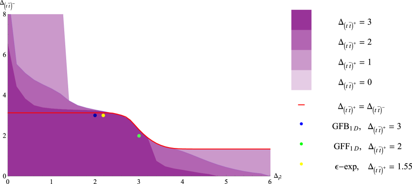
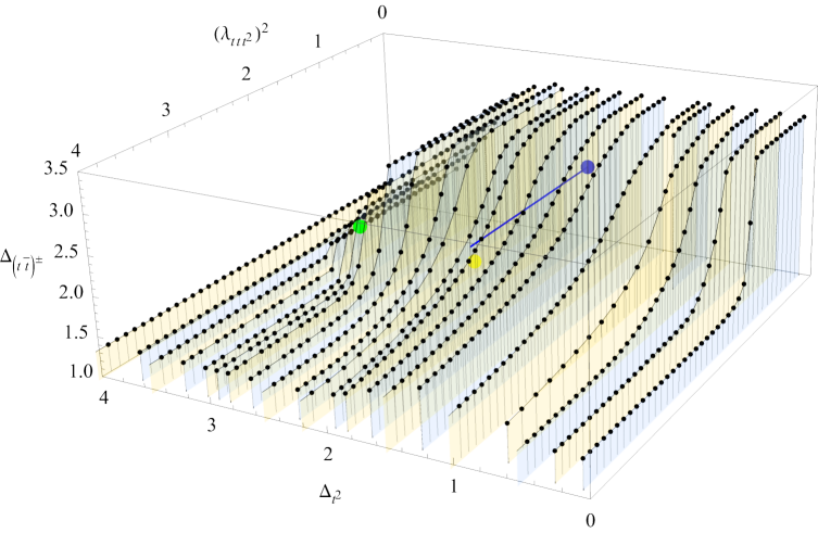
It was noted in [25] that the solution to the crossing equation of the generalized real free fermion ψ(τ1)ψ(τ2)ψ(τ3)ψ(τ4)delimited-⟨⟩𝜓subscript𝜏1𝜓subscript𝜏2𝜓subscript𝜏3𝜓subscript𝜏4\langle\psi(\tau_{1})\psi(\tau_{2})\psi(\tau_{3})\psi(\tau_{4})\rangle can be extended to a solution of the crossing equations in eq. (2.18), if the gap on the scaling dimension of the first operator in the traceless-symmetric representation does not exceed 2Δψ2subscriptΔ𝜓2\Delta_{\psi}. The spectra for the 𝒮𝒮{\mathcal{S}}-parity even and odd operators are equal in this case. For the displacement operator, this happens for ΔD2<2×2=4subscriptΔsuperscriptD2224\Delta_{{\text{D}^{2}}}<2\times 2=4, while for the tilt operator the solution appears for Δt2<2×1=2subscriptΔsuperscript𝑡2212\Delta_{t^{2}}<2\times 1=2.

2.3.3 Tilt and displacement

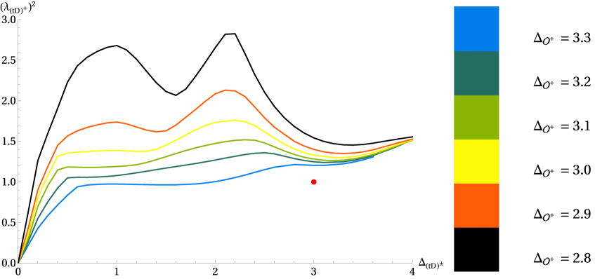
Next we consider a mixed system between the tilt operator t𝑡t and the displacement operator D, where we again use complex notation. In order to write down the crossing equations we note that the 𝒮𝒮\mathcal{S}-parity even singlets can appear both in t×t¯𝑡¯𝑡t\times\bar{t} and D×D¯D¯D\text{D}\times\bar{\text{D}}, while the 𝒮𝒮\mathcal{S}-parity odd channels are different in the two OPEs, because the tilt and displacement transform under different O(2)𝑂2O(2) groups. All in all, crossing reads

𝒪+(λtt¯𝒪\displaystyle\sum_{{\mathcal{O}}^{+}}(\lambda_{t\bar{t}{\mathcal{O}}} λDD¯𝒪)V+Δ(λtt¯𝒪λDD¯𝒪)+𝒪|λtt¯𝒪|2Vtt¯,Δ+𝒪|λDD¯𝒪|2VDD¯,Δ\displaystyle\;\lambda_{\text{D}\bar{\text{D}}{\mathcal{O}}})\vec{V}^{+}_{\Delta}\begin{pmatrix}\lambda_{t\bar{t}{\mathcal{O}}}\\ \lambda_{\text{D}\bar{\text{D}}{\mathcal{O}}}\end{pmatrix}+\sum_{{\mathcal{O}}^{-}}|\lambda_{t\bar{t}{\mathcal{O}}}|^{2}\vec{V}^{t\bar{t},-}_{\Delta}+\sum_{{\mathcal{O}}^{-}}|\lambda_{\text{D}\bar{\text{D}}{\mathcal{O}}}|^{2}\vec{V}^{\text{D}\bar{\text{D}},-}_{\Delta}
+𝒪+|λtt𝒪|2VΔtt+𝒪+|λDD𝒪|2VΔDD+𝒪±|λtD𝒪|2VΔ,StD=0.subscriptsuperscript𝒪superscriptsubscript𝜆𝑡𝑡𝒪2subscriptsuperscript𝑉𝑡𝑡Δsubscriptsuperscript𝒪superscriptsubscript𝜆DD𝒪2subscriptsuperscript𝑉DDΔsubscriptsuperscript𝒪plus-or-minussuperscriptsubscript𝜆𝑡D𝒪2subscriptsuperscript𝑉𝑡DΔ𝑆0\displaystyle+\sum_{{\mathcal{O}}^{+}}|\lambda_{tt{\mathcal{O}}}|^{2}\vec{V}^{tt}_{\Delta}+\sum_{{\mathcal{O}}^{+}}|\lambda_{\text{D}\text{D}{\mathcal{O}}}|^{2}\vec{V}^{\text{D}\text{D}}_{\Delta}+\sum_{{\mathcal{O}}^{\pm}}|\lambda_{t\text{D}{\mathcal{O}}}|^{2}\vec{V}^{t\text{D}}_{\Delta,S}=0\>. (2.22)

Once again the crossing vectors are presented in appendix B.2.

2.3.4 One real scalar and the tilt

The third setup we study is crossing for one real scalar ϕ1subscriptitalic-ϕ1\phi_{1} and a tilt operator t𝑡t, for which we use complex notation. This has applications to the magnetic line defect of section 3.2, where ϕ1subscriptitalic-ϕ1\phi_{1} corresponds to the scalar that breaks the bulk symmetry, and the tilt operator must be present due to the symmetry breaking. The numerical results for this setup will be discussed in section 4.3. The crossing equations can be obtain in a similar way as before, but we now obtain seven independent equations that in vector notation read

𝒪+subscriptsuperscript𝒪\displaystyle\sum_{{\mathcal{O}}^{+}} (λϕ1ϕ1𝒪λtt¯𝒪)VΔ+(λϕ1ϕ1𝒪λtt¯𝒪)+𝒪(λtt¯𝒪)2VΔ+𝒪+|λtt𝒪|2VΔtt+𝒪±|λϕ1t𝒪|2VΔ,Sϕ1t=0.subscript𝜆subscriptitalic-ϕ1subscriptitalic-ϕ1𝒪subscript𝜆𝑡¯𝑡𝒪subscriptsuperscript𝑉Δmatrixsubscript𝜆subscriptitalic-ϕ1subscriptitalic-ϕ1𝒪subscript𝜆𝑡¯𝑡𝒪subscriptsuperscript𝒪superscriptsubscript𝜆𝑡¯𝑡𝒪2subscriptsuperscript𝑉Δsubscriptsuperscript𝒪superscriptsubscript𝜆𝑡𝑡𝒪2subscriptsuperscript𝑉𝑡𝑡Δsubscriptsuperscript𝒪plus-or-minussuperscriptsubscript𝜆subscriptitalic-ϕ1𝑡𝒪2subscriptsuperscript𝑉subscriptitalic-ϕ1𝑡Δ𝑆0\displaystyle(\lambda_{\phi_{1}\phi_{1}{\mathcal{O}}}\;\lambda_{t\bar{t}{\mathcal{O}}})\vec{V}^{+}_{\Delta}\begin{pmatrix}\lambda_{\phi_{1}\phi_{1}{\mathcal{O}}}\\ \lambda_{t\bar{t}{\mathcal{O}}}\end{pmatrix}+\sum_{{\mathcal{O}}^{-}}(\lambda_{t\bar{t}{\mathcal{O}}})^{2}\vec{V}^{-}_{\Delta}+\sum_{{\mathcal{O}}^{+}}|\lambda_{tt{\mathcal{O}}}|^{2}\vec{V}^{tt}_{\Delta}+\sum_{{\mathcal{O}}^{\pm}}|\lambda_{\phi_{1}t{\mathcal{O}}}|^{2}\vec{V}^{\phi_{1}t}_{\Delta,S}=0\>. (2.23)

The crossing vectors are found in appendix B.3. Mutatis mutandis, the same system of crossing equations can be used to study the mixed correlators of ϕ1subscriptitalic-ϕ1\phi_{1} and D. We will leave this idea for future exploration.

2.3.5 Two complex scalars

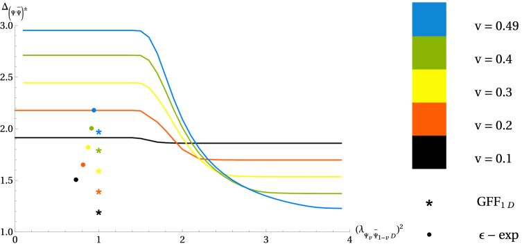
Finally we study the crossing equations of two unequal complex scalars ϕ1subscriptitalic-ϕ1\phi_{1} and ϕ2subscriptitalic-ϕ2\phi_{2}. We apply this to monodromy defects, see section 4.2, where ϕ1=ψn1+vsubscriptitalic-ϕ1subscript𝜓subscript𝑛1𝑣\phi_{1}=\psi_{n_{1}+v} and ϕ2=ψn2+vsubscriptitalic-ϕ2subscript𝜓subscript𝑛2𝑣\phi_{2}=\psi_{n_{2}+v} are two different defect modes of a bulk scalar field. In total there are twelve crossing equations and five different OPE channels [49]

𝒪±(λϕ1ϕ¯1𝒪\displaystyle\sum_{{\mathcal{O}}^{\pm}}(\lambda_{\phi_{1}\bar{\phi}_{1}{\mathcal{O}}} λϕ2ϕ¯2𝒪)VΔ,S(λϕ1ϕ¯1𝒪λϕ2ϕ¯2𝒪)+𝒪+|λϕ1ϕ1𝒪|2V11Δ+𝒪+|λϕ2ϕ2𝒪|2V22Δ\displaystyle\;\lambda_{\phi_{2}\bar{\phi}_{2}{\mathcal{O}}})\vec{V}_{\Delta,S}\begin{pmatrix}\lambda_{\phi_{1}\bar{\phi}_{1}{\mathcal{O}}}\\ \lambda_{\phi_{2}\bar{\phi}_{2}{\mathcal{O}}}\end{pmatrix}+\sum_{{\mathcal{O}}^{+}}|\lambda_{\phi_{1}\phi_{1}{\mathcal{O}}}|^{2}\vec{V}^{11}_{\Delta}+\sum_{{\mathcal{O}}^{+}}|\lambda_{\phi_{2}\phi_{2}{\mathcal{O}}}|^{2}\vec{V}^{22}_{\Delta}
+𝒪±|λϕ1ϕ2𝒪|2VΔ,S12+𝒪±|λϕ1ϕ¯2𝒪|2VΔ,S12¯=0.subscriptsuperscript𝒪plus-or-minussuperscriptsubscript𝜆subscriptitalic-ϕ1subscriptitalic-ϕ2𝒪2subscriptsuperscript𝑉12Δ𝑆subscriptsuperscript𝒪plus-or-minussuperscriptsubscript𝜆subscriptitalic-ϕ1subscript¯italic-ϕ2𝒪2subscriptsuperscript𝑉1¯2Δ𝑆0\displaystyle+\sum_{{\mathcal{O}}^{\pm}}|\lambda_{\phi_{1}\phi_{2}{\mathcal{O}}}|^{2}\vec{V}^{12}_{\Delta,S}+\sum_{{\mathcal{O}}^{\pm}}|\lambda_{\phi_{1}\bar{\phi}_{2}{\mathcal{O}}}|^{2}\vec{V}^{1\bar{2}}_{\Delta,S}=0\>. (2.24)

The crossing vectors can be found in appendix B.4.

Two complex generalized free fields.

The OPE coefficients that contain only ϕ1subscriptitalic-ϕ1\phi_{1} or only ϕ2subscriptitalic-ϕ2\phi_{2} follow from our discussion above. The new information is contained in the ϕ1×ϕ2subscriptitalic-ϕ1subscriptitalic-ϕ2\phi_{1}\times\phi_{2} OPE, which can be analyzed from the following four-point function

Gϕ1ϕ2ϕ¯2ϕ¯1(ξ)=ξΔ1+Δ2(1ξ)2Δ2=p=0cp(Δ1,Δ2)gΔ1+Δ2+pΔ12,Δ21(ξ).subscript𝐺subscriptitalic-ϕ1subscriptitalic-ϕ2subscript¯italic-ϕ2subscript¯italic-ϕ1𝜉superscript𝜉subscriptΔ1subscriptΔ2superscript1𝜉2subscriptΔ2superscriptsubscript𝑝0subscript𝑐𝑝subscriptΔ1subscriptΔ2superscriptsubscript𝑔subscriptΔ1subscriptΔ2𝑝subscriptΔ12subscriptΔ21𝜉\displaystyle\begin{split}G_{\phi_{1}\phi_{2}\bar{\phi}_{2}\bar{\phi}_{1}}(\xi)&=\frac{\xi^{\Delta_{1}+\Delta_{2}}}{(1-\xi)^{2\Delta_{2}}}=\sum_{p=0}^{\infty}c_{p}(\Delta_{1},\Delta_{2})g_{\Delta_{1}+\Delta_{2}+p}^{\Delta_{12},\Delta_{21}}(\xi)\>.\end{split} (2.25)

From here we immediately read off |λϕ1ϕ2𝒪|2superscriptsubscript𝜆subscriptitalic-ϕ1subscriptitalic-ϕ2𝒪2|\lambda_{\phi_{1}\phi_{2}{\mathcal{O}}}|^{2}, and by sending ϕ2ϕ¯2subscriptitalic-ϕ2subscript¯italic-ϕ2\phi_{2}\to\bar{\phi}_{2} we find that the same formula applies to |λϕ1ϕ¯2𝒪|2superscriptsubscript𝜆subscriptitalic-ϕ1subscript¯italic-ϕ2𝒪2|\lambda_{\phi_{1}\bar{\phi}_{2}{\mathcal{O}}}|^{2}.

3 Defect theories in the ε𝜀\varepsilon-expansion

In this section we use perturbation theory to study two important examples of conformal line defects: the SO(2)F𝑆𝑂subscript2𝐹SO(2)_{F}-preserving monodromy defect and the O(3)𝑂3O(3)-breaking magnetic line defect. We start by reviewing known results on the SO(2)F𝑆𝑂subscript2𝐹SO(2)_{F} monodromy defect in the ε𝜀\varepsilon-expansion, which has been studied in great detail in [38, 39, 40]. In view of the comparison to the numerical bootstrap results, we add a few OPE coefficients to the CFT data already available in the literature, which can be straightforwardly extracted from the results of [39]. Then, we study the magnetic line defect in the ε𝜀\varepsilon-expansion, and present new results which complement the study performed in [5]. We compare these perturbative results with the predictions from the numerical conformal bootstrap in section 4.

3.1 Monodromy defects with SO(2)F𝑆𝑂subscript2𝐹SO(2)_{F} symmetry

Monodromy defects in the free O(2)𝑂2O(2) model.

The first example we discuss is a U(1)F𝑈subscript1𝐹U(1)_{F}-preserving monodromy defect in free theory. This defect, first considered in [38, 39, 40], generalizes the 2subscript2\mathbb{Z}_{2} twist defect defined in [2, 25]. Following [38], we start from a set of N=2𝑁2N=2 free real scalars ϕisuperscriptitalic-ϕ𝑖\phi^{i} in the bulk that satisfy

ϕi(r,θ+2π,x)=gijϕj(r,θ,x),gijO(2)F.formulae-sequencesuperscriptitalic-ϕ𝑖𝑟𝜃2𝜋𝑥superscript𝑔𝑖𝑗superscriptitalic-ϕ𝑗𝑟𝜃𝑥superscript𝑔𝑖𝑗𝑂subscript2𝐹\phi^{i}(r,\theta+2\pi,\vec{x})=g^{ij}\phi^{j}(r,\theta,\vec{x})\>,\quad g^{ij}\in O(2)_{F}\>. (3.1)

The scalars ϕisuperscriptitalic-ϕ𝑖\phi^{i} either get mixed into each other, obtain a minus sign, or remain unchanged when going around the monodromy defect. In terms of the complex combination

Φ=ϕ1+iϕ2,Φsuperscriptitalic-ϕ1𝑖superscriptitalic-ϕ2\Phi=\phi^{1}+i\phi^{2}\>, (3.2)

the most general U(1)F𝑈subscript1𝐹U(1)_{F} monodromy becomes101010As explained in [40] this monodromy can be thought of as a large and constant U(1)𝑈1U(1) background gauge transformation for ΦΦ\Phi.

Φ(r,θ+2π,x)=e2πivΦ(r,θ,x),vv+1,v[0,1).formulae-sequenceΦ𝑟𝜃2𝜋𝑥superscript𝑒2𝜋𝑖𝑣Φ𝑟𝜃𝑥formulae-sequencesimilar-to𝑣𝑣1𝑣01\Phi(r,\theta+2\pi,\vec{x})=e^{2\pi iv}\Phi(r,\theta,\vec{x})\>,\quad v\sim v+1~{},\quad v\in[0,1)~{}. (3.3)

The complex scalar ΦΦ\Phi has an internal U(1)F𝑈subscript1𝐹U(1)_{F} symmetry that gets enhanced to O(2)F𝑂subscript2𝐹O(2)_{F} for v=0𝑣0v=0 (the trivial defect) and for v=12𝑣12v=\frac{1}{2} (the 2subscript2\mathbb{Z}_{2} monodromy defect). For these values of v𝑣v, the transformation ΦΦ¯Φ¯Φ\Phi\to\bar{\Phi}, which belongs to O(2)F𝑂subscript2𝐹O(2)_{F} but not U(1)SO(2)Fsimilar-to-or-equals𝑈1𝑆𝑂subscript2𝐹U(1)\simeq SO(2)_{F}, is a symmetry. As a consequence of the monodromy, the local primary operators allowed to appear in the bulk-defect expansion of ΦΦ\Phi will generically have non-integer spin s+v𝑠𝑣s\in\mathbb{Z}+v, i.e.

Φ(r,θ,x)r0Ψss+veiθsrΔΦΔΨsΨs(x)+c.c.Φ𝑟𝜃𝑥𝑟0similar-tosubscriptsubscriptΨ𝑠subscript𝑠𝑣superscript𝑒𝑖𝜃𝑠superscript𝑟subscriptΔΦsubscriptΔsubscriptΨ𝑠subscriptΨ𝑠𝑥c.c.\displaystyle\Phi(r,\theta,\vec{x})\underset{r\rightarrow 0}{\sim}\sum_{\Psi_{s}}\sum_{s\in\mathbb{Z}+v}\frac{e^{-i\theta s}}{r^{\Delta_{\Phi}-\Delta_{\Psi_{s}}}}\Psi_{s}(\vec{x})+\text{c.c.} (3.4)

The scaling dimensions of the defect modes of ΦΦ\Phi are completely fixed as a consequence of the bulk free equation of motion, and read (see e.g. [2, 25, 41])

ΔΨs=ΔΦ+|s|=d22+|s|.subscriptΔsubscriptΨ𝑠subscriptΔΦ𝑠𝑑22𝑠\displaystyle\Delta_{\Psi_{s}}=\Delta_{\Phi}+|s|=\frac{d-2}{2}+|s|\,. (3.5)

In terms of real bulk scalar ϕiseisθψsi+c.c.similar-tosuperscriptitalic-ϕ𝑖subscript𝑠superscript𝑒𝑖𝑠𝜃superscriptsubscript𝜓𝑠𝑖c.c.\phi^{i}\sim\sum_{s}e^{is\theta}\psi_{s}^{i}+\text{c.c.}, the reality condition is that ψ¯si=ψsisuperscriptsubscript¯𝜓𝑠𝑖superscriptsubscript𝜓𝑠𝑖\bar{\psi}_{s}^{i}=\psi_{-s}^{i} and so Ψs=ψs1+iψs2subscriptΨ𝑠subscriptsuperscript𝜓1𝑠𝑖subscriptsuperscript𝜓2𝑠\Psi_{s}=\psi^{1}_{s}+i\psi^{2}_{s} satisfies Ψ¯sψ¯s1iψ¯s2=ψs1iψs2subscript¯Ψ𝑠subscriptsuperscript¯𝜓1𝑠𝑖subscriptsuperscript¯𝜓2𝑠subscriptsuperscript𝜓1𝑠𝑖subscriptsuperscript𝜓2𝑠\bar{\Psi}_{s}\equiv\bar{\psi}^{1}_{s}-i\bar{\psi}^{2}_{s}=\psi^{1}_{-s}-i\psi^{2}_{-s}.

Monodromy defects in the interacting O(2)𝑂2O(2) model.

The simplest example of an interacting U(1)F𝑈subscript1𝐹U(1)_{F} monodromy defect is obtained by imposing the condition of eq. (3.3) on the fundamental vector of the critical 3d O(2)𝑂2O(2) vector model. In perturbation theory this example is tractable in the standard framework of ε𝜀\varepsilon-expansion (with fixed co-dimension q=2𝑞2q=2). The bulk is tuned to the Wilson-Fisher fixed point with coupling111111There is a slight difference in notation with respect to [39], where the symmetry group in the bulk and on the defect is O(2N)𝑂2𝑁O(2N), while we will denote it by O(N)𝑂𝑁O(N) with N=𝑁absentN= even, and in particular take N=2𝑁2N=2, to avoid differences in notation throughout the paper.

λ=8π210+O(ε2).superscript𝜆8superscript𝜋210𝑂superscript𝜀2\lambda^{*}=\frac{8\pi^{2}}{10}+O(\varepsilon^{2})\>. (3.6)

The scaling dimensions of the defect modes ΨssubscriptΨ𝑠\Psi_{s} are found to be [38, 39]

ΔΨs=1+|s|ε2+15v(v1)|s|ε+O(ε2).subscriptΔsubscriptΨ𝑠1𝑠𝜀215𝑣𝑣1𝑠𝜀𝑂superscript𝜀2\Delta_{\Psi_{s}}=1+|s|-\frac{\varepsilon}{2}+\frac{1}{5}\frac{v(v-1)}{|s|}\varepsilon+O(\varepsilon^{2})\>. (3.7)

For the monodromy defect, the displacement operator D appears in the OPE of two defect modes with spins |s|=v𝑠𝑣|s|=v and |s|=v1𝑠𝑣1|s|=v-1:

Ψv×Ψ¯v1D,Ψ¯v×Ψv1D¯.formulae-sequencesimilar-tosubscriptΨ𝑣subscript¯Ψ𝑣1Dsimilar-tosubscript¯Ψ𝑣subscriptΨ𝑣1¯D\displaystyle\Psi_{v}\times\bar{\Psi}_{v-1}\sim\text{D}~{},\quad\bar{\Psi}_{v}\times{\Psi}_{v-1}\sim{\bar{\text{D}}}~{}. (3.8)

In appendix A we show that it appears in the Ψv×Ψ¯v1subscriptΨ𝑣subscript¯Ψ𝑣1\Psi_{v}\times\bar{\Psi}_{v-1} OPE with (squared) OPE coefficient

|λΨvΨ¯v1D|2=1+ε10(2H1v+2Hv3),superscriptsubscript𝜆subscriptΨ𝑣subscript¯Ψ𝑣1D21𝜀102superscript𝐻1𝑣2superscript𝐻𝑣3|\lambda_{\Psi_{v}\bar{\Psi}_{v-1}\text{D}}|^{2}=1+\frac{\varepsilon}{10}\left(2H^{1-v}+2H^{v}-3\right)\>, (3.9)

where Hvsuperscript𝐻𝑣H^{v} is the analytic continuation of the harmonic number. We will also need the scaling dimensions and correponding OPE coefficients of the leading singlets in

Ψv×Ψ¯v𝟙+𝒪0+,Ψv1×Ψ¯v1𝟙+𝒪0+.formulae-sequencesimilar-tosubscriptΨ𝑣subscript¯Ψ𝑣1subscript𝒪0similar-tosubscriptΨ𝑣1subscript¯Ψ𝑣11subscript𝒪0\displaystyle\Psi_{v}\times\bar{\Psi}_{v}\sim{\mathds{1}}+\mathcal{O}_{0}+\dots,\quad\Psi_{v-1}\times\bar{\Psi}_{v-1}\sim{\mathds{1}}+\mathcal{O}_{0}+\dots. (3.10)

In appendix A we show that

Δ𝒪0=2+2vε+ε(45(1+2v)+2(v1)5).subscriptΔsubscript𝒪022𝑣𝜀𝜀4512𝑣2𝑣15\displaystyle\Delta_{\mathcal{O}_{0}}=2+2v-\varepsilon+\varepsilon\left(\frac{4}{5(1+2v)}+\frac{2(v-1)}{5}\right)~{}. (3.11)

In section 4.2 we will compare the ε𝜀\varepsilon-expansion predictions to the numerical bootstrap results.

It would be interesting to compute the correlator DDD¯D¯delimited-⟨⟩DD¯D¯D\langle\text{D}\text{D}{\bar{\text{D}}}{\bar{\text{D}}}\rangle at the first non-trivial order in ε𝜀\varepsilon-expansion to compare this to our single-correlator numerical bounds for the displacement operator. We will leave this for future work.

3.2 Localized magnetic field line defect

Let us continue with the determination of three-point OPE coefficients of defect operators for the magnetic line defect. The calculation is based on and extends the work [5], which focused on the scaling dimensions of low-lying defect operators. We obtain these results from a Feynman diagram expansion, keeping terms up to order O(ε)𝑂𝜀O(\varepsilon) in the ε𝜀\varepsilon-expansion. In order to obtain properly normalized OPE coefficients, we need to determine both two- and three-point functions. At the end, we also calculate several four-point functions, that by means of the conformal block decomposition allow us to check our results and obtain further coefficients.

3.2.1 Overview

To study the magnetic line defect we use a Lagrangian description that couples the O(N)𝑂𝑁O(N) model to a magnetic field localized along an infinite line. Using rotation invariance we take the line to be oriented as xμ(τ)=(τ,0)superscript𝑥𝜇𝜏𝜏0x^{\mu}(\tau)=(\tau,\vec{0}), while using O(N)𝑂𝑁O(N) invariance, we choose the magnetic field to be in the ϕ1subscriptitalic-ϕ1\phi_{1} direction. All in all, the action is

S=ddx(12(μϕa)2+λ04!(ϕa2)2)+h0𝑑τϕ1(x(τ)),a=1,,N.formulae-sequence𝑆superscript𝑑𝑑𝑥12superscriptsubscript𝜇subscriptitalic-ϕ𝑎2subscript𝜆04superscriptsuperscriptsubscriptitalic-ϕ𝑎22subscript0superscriptsubscriptdifferential-d𝜏subscriptitalic-ϕ1𝑥𝜏𝑎1𝑁\displaystyle S=\int d^{d}x\left(\frac{1}{2}(\partial_{\mu}\phi_{a})^{2}+\frac{\lambda_{0}}{4!}(\phi_{a}^{2})^{2}\right)+h_{0}\int_{-\infty}^{\infty}d\tau\,\phi_{1}(x(\tau))\,,\qquad a=1,\ldots,N\,. (3.12)

Let us start reviewing the results of [5], which motivate our bootstrap setup in section 4.3. Because the defect in eq. (3.12) breaks the global symmetry O(N)O(N1)𝑂𝑁𝑂𝑁1O(N)\to O(N-1), there exists a tilt operator besides the displacement operator. In perturbation theory, the tilt and displacement operators are identified as

ta^ϕa^,Dϕ1,a^=2,,N,formulae-sequenceproportional-tosubscript𝑡^𝑎subscriptitalic-ϕ^𝑎formulae-sequenceproportional-toDsubscriptitalic-ϕ1^𝑎2𝑁\displaystyle t_{\hat{a}}\propto\phi_{\hat{a}}\,,\qquad\text{D}\propto\nabla\phi_{1}\,,\qquad\hat{a}=2,\ldots,N\,, (3.13)

and as usual they have protected dimension Δt=1subscriptΔ𝑡1\Delta_{t}=1 and ΔD=2subscriptΔD2\Delta_{\text{D}}=2. After the tilt, the operator with the second-lowest dimension is the localized magnetic field ϕ1subscriptitalic-ϕ1\phi_{1}. The scaling dimension of ϕ1subscriptitalic-ϕ1\phi_{1} to two-loop order in the ε𝜀\varepsilon-expansion reads

Δϕ1=1+ε3N2+49N+1942(N+8)2ε2+O(ε3)Padé 1.55.subscriptΔsubscriptitalic-ϕ11𝜀3superscript𝑁249𝑁1942superscript𝑁82superscript𝜀2𝑂superscript𝜀3Padé1.55\displaystyle\Delta_{\phi_{1}}=1+\varepsilon-\frac{3N^{2}+49N+194}{2(N+8)^{2}}\varepsilon^{2}+O(\varepsilon^{3})\;\;\xrightarrow{\text{Pad\'{e}}}\;1.55\,. (3.14)

Furthermore, inputting information from d=2𝑑2d=2 in a Padé approximant, the authors of [5] estimated the value Δϕ11.55subscriptΔsubscriptitalic-ϕ11.55\Delta_{\phi_{1}}\approx 1.55, which is also consistent with their 1/N1𝑁1/N results and Monte-Carlo simulations [50, 51].

Since the two lowest-dimensional operators on the defect are ta^subscript𝑡^𝑎t_{\hat{a}} and ϕ1subscriptitalic-ϕ1\phi_{1}, a natural candidate for a bootstrap study is the mixed correlator involving them, which is the one-dimensional analog of [52, 53]. In order to motivate gap assumptions in the numerical study, let us look at the lowest-lying operators in the different OPE channels. In the singlet channel (S)𝑆(S), which appears for ϕ1×ϕ1subscriptitalic-ϕ1subscriptitalic-ϕ1\phi_{1}\times\phi_{1} or (ta^×tb^)Ssubscriptsubscript𝑡^𝑎subscript𝑡^𝑏𝑆(t_{\hat{a}}\times t_{\hat{b}})_{S}, the lowest dimension operators are ϕ1+s+s++subscriptitalic-ϕ1subscript𝑠subscript𝑠\phi_{1}+s_{-}+s_{+}+\ldots. Here s±subscript𝑠plus-or-minuss_{\pm} are linear combinations of ϕ12superscriptsubscriptitalic-ϕ12\phi_{1}^{2} and ϕa2superscriptsubscriptitalic-ϕ𝑎2\phi_{a}^{2} with scaling dimension

Δs±subscriptΔsubscript𝑠plus-or-minus\displaystyle\Delta_{s_{\pm}} =2+ε3N+20±N2+40N+3202(N+8)+O(ε2).absent2𝜀plus-or-minus3𝑁20superscript𝑁240𝑁3202𝑁8𝑂superscript𝜀2\displaystyle=2+\varepsilon\,\frac{3N+20\pm\sqrt{N^{2}+40N+320}}{2(N+8)}+O(\varepsilon^{2})\,. (3.15)

Similarly, vector operators appear in the OPE ϕ1×ta^=ta^+Va^+subscriptitalic-ϕ1subscript𝑡^𝑎subscript𝑡^𝑎subscript𝑉^𝑎\phi_{1}\times t_{\hat{a}}=t_{\hat{a}}+V_{\hat{a}}+\ldots. The leading vector is Va^ϕ1ϕa^proportional-tosubscript𝑉^𝑎subscriptitalic-ϕ1subscriptitalic-ϕ^𝑎V_{\hat{a}}\propto\phi_{1}\phi_{\hat{a}}, and its dimension reads

ΔVsubscriptΔ𝑉\displaystyle\Delta_{V} =2+εN+10N+8+O(ε2).absent2𝜀𝑁10𝑁8𝑂superscript𝜀2\displaystyle=2+\varepsilon\,\frac{N+10}{N+8}+O(\varepsilon^{2})\>. (3.16)

Finally, in the OPE ta^×tb^subscript𝑡^𝑎subscript𝑡^𝑏t_{\hat{a}}\times t_{\hat{b}} there is an antisymmetric channel (A)𝐴(A), where the lowest-dimensional operator is Aa^b^ϕ[a^ϕb^]A_{\hat{a}\hat{b}}\propto\phi_{[\hat{a}}\phi_{\hat{b}]}, and a symmetric-traceless channel (T)𝑇(T) with the lowest-lying operator Ta^b^ϕa^ϕb^proportional-tosubscript𝑇^𝑎^𝑏subscriptitalic-ϕ^𝑎subscriptitalic-ϕ^𝑏T_{\hat{a}\hat{b}}\propto\phi_{\hat{a}}\phi_{\hat{b}}. Their dimensions are given by

ΔA=3+O(ε2),ΔT=2+2εN+8+O(ε2).formulae-sequencesubscriptΔ𝐴3𝑂superscript𝜀2subscriptΔ𝑇22𝜀𝑁8𝑂superscript𝜀2\displaystyle\Delta_{A}=3+O(\varepsilon^{2})\,,\qquad\Delta_{T}=2+\frac{2\varepsilon}{N+8}+O(\varepsilon^{2})\>. (3.17)

Besides scaling dimensions, the numerical conformal bootstrap can also probe the three-point OPE coefficients of these operators. The goal of the rest of the section will be to compute these OPE coefficients to leading order in the ε𝜀\varepsilon-expansion, see table 1 for a summary of the main results. Besides two- and three-point functions, we also compute several four-point functions, which thanks to the conformal block decomposition, contain information of many other OPE coefficients.

λϕ1ϕ1ϕ1subscript𝜆subscriptitalic-ϕ1subscriptitalic-ϕ1subscriptitalic-ϕ1\lambda_{\phi_{1}\phi_{1}\phi_{1}} λttϕ1subscript𝜆𝑡𝑡subscriptitalic-ϕ1\lambda_{tt\phi_{1}} λϕ1ϕ1s±subscript𝜆subscriptitalic-ϕ1subscriptitalic-ϕ1subscript𝑠plus-or-minus\lambda_{\phi_{1}\phi_{1}s_{\pm}} λtts±subscript𝜆𝑡𝑡subscript𝑠plus-or-minus\lambda_{tts_{\pm}} λϕ1tVsubscript𝜆subscriptitalic-ϕ1𝑡𝑉\lambda_{\phi_{1}tV} λttAsubscript𝜆𝑡𝑡𝐴\lambda_{ttA} λttTsubscript𝜆𝑡𝑡𝑇\lambda_{ttT}
 (3.50)  (3.50)  (3.55)  (3.56)  (3.57)  (3.62)  (3.57)
Table 1: Summary of the most important OPE coefficients computed in this section. Further coefficients appear in (3.52) or can be extracted from the four-point functions in section 3.2.5.

3.2.2 Conventions

Throughout this section we follow the conventions of [5], so in particular the action is given by eq. (3.12) and the scalar propagator in free theory is

ϕa(x1)ϕb(x2)λ0=h0=0=κδab(x122)1ε2,κ=Γ(d2)2πd/2(d2).formulae-sequencesubscriptdelimited-⟨⟩subscriptitalic-ϕ𝑎subscript𝑥1subscriptitalic-ϕ𝑏subscript𝑥2subscript𝜆0subscript00𝜅subscript𝛿𝑎𝑏superscriptsuperscriptsubscript𝑥1221𝜀2𝜅Γ𝑑22superscript𝜋𝑑2𝑑2\displaystyle\leavevmode\hbox to23.16pt{\vbox to0.4pt{\pgfpicture\makeatletter\hbox{\hskip 0.2pt\lower-0.2pt\hbox to0.0pt{\pgfsys@beginscope\pgfsys@invoke{ }\definecolor{pgfstrokecolor}{rgb}{0,0,0}\pgfsys@color@rgb@stroke{0}{0}{0}\pgfsys@invoke{ }\pgfsys@color@rgb@fill{0}{0}{0}\pgfsys@invoke{ }\pgfsys@setlinewidth{0.4pt}\pgfsys@invoke{ }\nullfont\hbox to0.0pt{\pgfsys@beginscope\pgfsys@invoke{ } {}{{}}{} {}{}\pgfsys@beginscope\pgfsys@invoke{ }\pgfsys@setdash{3.0pt,3.0pt}{0.0pt}\pgfsys@invoke{ }{}\pgfsys@moveto{0.0pt}{0.0pt}\pgfsys@lineto{22.76228pt}{0.0pt}\pgfsys@stroke\pgfsys@invoke{ } \pgfsys@invoke{\lxSVG@closescope }\pgfsys@endscope \pgfsys@invoke{\lxSVG@closescope }\pgfsys@endscope{{ {}{}{}{}{}}{{{}}{{}}}}{}{}\hss}\pgfsys@discardpath\pgfsys@invoke{\lxSVG@closescope }\pgfsys@endscope\hss}}\lxSVG@closescope\endpgfpicture}}\;\,\equiv\;\langle\phi_{a}(x_{1})\phi_{b}(x_{2})\rangle_{\lambda_{0}=h_{0}=0}\,=\;\frac{\kappa\delta_{ab}}{(x_{12}^{2})^{1-\frac{\varepsilon}{2}}}\,,\qquad\kappa=\frac{\Gamma\!\left(\frac{d}{2}\right)}{2\pi^{d/2}(d-2)}\,. (3.18)

In perturbative expansions there is a bulk four-point vertex and a vertex that couples a bulk operator to the defect

λ0ddx,h0𝑑τ.formulae-sequencesubscript𝜆0superscript𝑑𝑑𝑥subscript0superscriptsubscriptdifferential-d𝜏\displaystyle\leavevmode\hbox to11.78pt{\vbox to11.78pt{\pgfpicture\makeatletter\hbox{\hskip 5.89046pt\lower-5.89046pt\hbox to0.0pt{\pgfsys@beginscope\pgfsys@invoke{ }\definecolor{pgfstrokecolor}{rgb}{0,0,0}\pgfsys@color@rgb@stroke{0}{0}{0}\pgfsys@invoke{ }\pgfsys@color@rgb@fill{0}{0}{0}\pgfsys@invoke{ }\pgfsys@setlinewidth{0.4pt}\pgfsys@invoke{ }\nullfont\hbox to0.0pt{\pgfsys@beginscope\pgfsys@invoke{ } {}{{}}{} {}{}\pgfsys@beginscope\pgfsys@invoke{ }\pgfsys@setdash{3.0pt,3.0pt}{0.0pt}\pgfsys@invoke{ }{}\pgfsys@moveto{5.69046pt}{5.69046pt}\pgfsys@lineto{-5.69046pt}{-5.69046pt}\pgfsys@stroke\pgfsys@invoke{ } \pgfsys@invoke{\lxSVG@closescope }\pgfsys@endscope{}{{}}{} {}{}\pgfsys@beginscope\pgfsys@invoke{ }\pgfsys@setdash{3.0pt,3.0pt}{0.0pt}\pgfsys@invoke{ }{}\pgfsys@moveto{-5.69046pt}{5.69046pt}\pgfsys@lineto{5.69046pt}{-5.69046pt}\pgfsys@stroke\pgfsys@invoke{ } \pgfsys@invoke{\lxSVG@closescope }\pgfsys@endscope{{}}\hbox{\hbox{{\pgfsys@beginscope\pgfsys@invoke{ }\definecolor[named]{pgfstrokecolor}{rgb}{0,0,0}\pgfsys@color@gray@stroke{0}\pgfsys@invoke{ }\definecolor[named]{pgffillcolor}{rgb}{0,0,0}\pgfsys@color@gray@fill{0}\pgfsys@invoke{ }{{}{{{}}}{{}}{}{}{}{}{}{}{}{}{}{\pgfsys@beginscope\pgfsys@invoke{ }\definecolor[named]{pgfstrokecolor}{rgb}{0,0,0}\pgfsys@color@gray@stroke{0}\pgfsys@invoke{ }\definecolor[named]{pgffillcolor}{rgb}{0,0,0}\pgfsys@color@gray@fill{0}\pgfsys@invoke{ }{}\pgfsys@moveto{1.4143pt}{0.0pt}\pgfsys@curveto{1.4143pt}{0.7811pt}{0.7811pt}{1.4143pt}{0.0pt}{1.4143pt}\pgfsys@curveto{-0.7811pt}{1.4143pt}{-1.4143pt}{0.7811pt}{-1.4143pt}{0.0pt}\pgfsys@curveto{-1.4143pt}{-0.7811pt}{-0.7811pt}{-1.4143pt}{0.0pt}{-1.4143pt}\pgfsys@curveto{0.7811pt}{-1.4143pt}{1.4143pt}{-0.7811pt}{1.4143pt}{0.0pt}\pgfsys@closepath\pgfsys@moveto{0.0pt}{0.0pt}\pgfsys@fillstroke\pgfsys@invoke{ } \pgfsys@invoke{\lxSVG@closescope }\pgfsys@endscope}{{{{}}\pgfsys@beginscope\pgfsys@invoke{ }\pgfsys@transformcm{1.0}{0.0}{0.0}{1.0}{0.0pt}{0.0pt}\pgfsys@invoke{ }\hbox{{\definecolor{pgfstrokecolor}{rgb}{0,0,0}\pgfsys@color@rgb@stroke{0}{0}{0}\pgfsys@invoke{ }\pgfsys@color@rgb@fill{0}{0}{0}\pgfsys@invoke{ }\hbox{} }}\pgfsys@invoke{\lxSVG@closescope }\pgfsys@endscope}}} \pgfsys@invoke{\lxSVG@closescope }\pgfsys@endscope}}} \pgfsys@invoke{\lxSVG@closescope }\pgfsys@endscope{{ {}{}{}{}{}}{{{}}{{}}}}{}{}\hss}\pgfsys@discardpath\pgfsys@invoke{\lxSVG@closescope }\pgfsys@endscope\hss}}\lxSVG@closescope\endpgfpicture}}\;\;\equiv\;-\lambda_{0}\int d^{d}x\ldots\,,\qquad\leavevmode\hbox to23.56pt{\vbox to18.89pt{\pgfpicture\makeatletter\hbox{\hskip 3.24544pt\lower-1.6143pt\hbox to0.0pt{\pgfsys@beginscope\pgfsys@invoke{ }\definecolor{pgfstrokecolor}{rgb}{0,0,0}\pgfsys@color@rgb@stroke{0}{0}{0}\pgfsys@invoke{ }\pgfsys@color@rgb@fill{0}{0}{0}\pgfsys@invoke{ }\pgfsys@setlinewidth{0.4pt}\pgfsys@invoke{ }\nullfont\hbox to0.0pt{\pgfsys@beginscope\pgfsys@invoke{ } {}{{}}{} {}{}\pgfsys@beginscope\pgfsys@invoke{ }\pgfsys@setlinewidth{0.8pt}\pgfsys@invoke{ }{}\pgfsys@moveto{-2.84544pt}{0.0pt}\pgfsys@lineto{19.91684pt}{0.0pt}\pgfsys@stroke\pgfsys@invoke{ } \pgfsys@invoke{\lxSVG@closescope }\pgfsys@endscope{}{{}}{} {}{}\pgfsys@beginscope\pgfsys@invoke{ }\pgfsys@setdash{3.0pt,3.0pt}{0.0pt}\pgfsys@invoke{ }{}\pgfsys@moveto{8.5359pt}{0.0pt}\pgfsys@lineto{8.5359pt}{17.07182pt}\pgfsys@stroke\pgfsys@invoke{ } \pgfsys@invoke{\lxSVG@closescope }\pgfsys@endscope{{}}\hbox{\hbox{{\pgfsys@beginscope\pgfsys@invoke{ }\definecolor[named]{pgfstrokecolor}{rgb}{0,0,1}\pgfsys@color@rgb@stroke{0}{0}{1}\pgfsys@invoke{ }\definecolor[named]{pgffillcolor}{rgb}{0,0,1}\pgfsys@color@rgb@fill{0}{0}{1}\pgfsys@invoke{ }{{}{{{}}}{{}}{}{}{}{}{}{}{}{}{}{\pgfsys@beginscope\pgfsys@invoke{ }\definecolor[named]{pgfstrokecolor}{rgb}{0,0,1}\pgfsys@color@rgb@stroke{0}{0}{1}\pgfsys@invoke{ }\definecolor[named]{pgffillcolor}{rgb}{0,0,1}\pgfsys@color@rgb@fill{0}{0}{1}\pgfsys@invoke{ }{}\pgfsys@moveto{9.95021pt}{0.0pt}\pgfsys@curveto{9.95021pt}{0.7811pt}{9.317pt}{1.4143pt}{8.5359pt}{1.4143pt}\pgfsys@curveto{7.7548pt}{1.4143pt}{7.1216pt}{0.7811pt}{7.1216pt}{0.0pt}\pgfsys@curveto{7.1216pt}{-0.7811pt}{7.7548pt}{-1.4143pt}{8.5359pt}{-1.4143pt}\pgfsys@curveto{9.317pt}{-1.4143pt}{9.95021pt}{-0.7811pt}{9.95021pt}{0.0pt}\pgfsys@closepath\pgfsys@moveto{8.5359pt}{0.0pt}\pgfsys@fillstroke\pgfsys@invoke{ } \pgfsys@invoke{\lxSVG@closescope }\pgfsys@endscope}{{{{}}\pgfsys@beginscope\pgfsys@invoke{ }\pgfsys@transformcm{1.0}{0.0}{0.0}{1.0}{8.5359pt}{0.0pt}\pgfsys@invoke{ }\hbox{{\definecolor{pgfstrokecolor}{rgb}{0,0,0}\pgfsys@color@rgb@stroke{0}{0}{0}\pgfsys@invoke{ }\pgfsys@color@rgb@fill{0}{0}{0}\pgfsys@invoke{ }\hbox{} }}\pgfsys@invoke{\lxSVG@closescope }\pgfsys@endscope}}} \pgfsys@invoke{\lxSVG@closescope }\pgfsys@endscope}}} \pgfsys@invoke{\lxSVG@closescope }\pgfsys@endscope{{ {}{}{}{}{}}{{{}}{{}}}}{}{}\hss}\pgfsys@discardpath\pgfsys@invoke{\lxSVG@closescope }\pgfsys@endscope\hss}}\lxSVG@closescope\endpgfpicture}}\;\;\equiv\;-h_{0}\int_{-\infty}^{\infty}d\tau\ldots\,. (3.19)

Notice that only ϕ1subscriptitalic-ϕ1\phi_{1} couples to the line, and not all ϕa^subscriptitalic-ϕ^𝑎\phi_{\hat{a}} for a^=2,,N^𝑎2𝑁\hat{a}=2,\ldots,N. We work in dimensional regularization with minimal subtraction, so the bare couplings λ0subscript𝜆0\lambda_{0} and h0subscript0h_{0} are related to the renormalized ones as

λ0=λMε(1+λ(4π)2N+83ε+O(λ2)),h0=hMε/2(1+λ(4π)2h212ε+O(λ2)).formulae-sequencesubscript𝜆0𝜆superscript𝑀𝜀1𝜆superscript4𝜋2𝑁83𝜀𝑂superscript𝜆2subscript0superscript𝑀𝜀21𝜆superscript4𝜋2superscript212𝜀𝑂superscript𝜆2\displaystyle\lambda_{0}=\lambda M^{\varepsilon}\left(1+\frac{\lambda}{(4\pi)^{2}}\frac{N+8}{3\varepsilon}+O(\lambda^{2})\right)\,,\quad h_{0}=hM^{\varepsilon/2}\left(1+\frac{\lambda}{(4\pi)^{2}}\frac{h^{2}}{12\varepsilon}+O(\lambda^{2})\right)\,. (3.20)

The renormalized couplings depend on the renormalization scale M𝑀M as

βλsubscript𝛽𝜆\displaystyle\beta_{\lambda} =MdλdM=λε+λ2(4π)2N+83+O(λ3),absent𝑀𝑑𝜆𝑑𝑀𝜆𝜀superscript𝜆2superscript4𝜋2𝑁83𝑂superscript𝜆3\displaystyle=M\frac{d\lambda}{dM}=-\lambda\varepsilon+\frac{\lambda^{2}}{(4\pi)^{2}}\frac{N+8}{3}+O(\lambda^{3})\,,
βhsubscript𝛽\displaystyle\beta_{h} =MdhdM=hε2+λ(4π)2h36+O(λ2),absent𝑀𝑑𝑑𝑀𝜀2𝜆superscript4𝜋2superscript36𝑂superscript𝜆2\displaystyle=M\frac{dh}{dM}=-\frac{h\varepsilon}{2}+\frac{\lambda}{(4\pi)^{2}}\frac{h^{3}}{6}+O(\lambda^{2})\,, (3.21)

so there exists a non-trivial fixed point where we evaluate most of our results:

λ(4π)2=3εN+8+O(ε2),h2=N+8+O(ε).formulae-sequencesubscript𝜆superscript4𝜋23𝜀𝑁8𝑂superscript𝜀2superscriptsubscript2𝑁8𝑂𝜀\displaystyle\frac{\lambda_{*}}{(4\pi)^{2}}=\frac{3\varepsilon}{N+8}+O(\varepsilon^{2})\,,\qquad h_{*}^{2}=N+8+O(\varepsilon)\,. (3.22)

Since we are interested in obtaining OPE coefficients at order O(ε)𝑂𝜀O(\varepsilon), we shall consider diagrams with at most one bulk vertex insertion λO(ε)similar-tosubscript𝜆𝑂𝜀\lambda_{*}\sim O(\varepsilon). On the other hand, we have to allow an arbitrary number of defect insertions because hO(1)similar-tosubscript𝑂1h_{*}\sim O(1). However, in practice only a finite number of diagrams will contribute at any given order in ε𝜀\varepsilon.

We often split the coordinates into a direction τ𝜏\tau parallel to the defect and xd1𝑥superscript𝑑1\vec{x}\in\mathbb{R}^{d-1} directions orthogonal to the defect. We shall only consider correlation functions of operators that live on the defect, for which we use the shorthand notation 𝒪(τ)=𝒪(τ,x=0)𝒪𝜏𝒪𝜏𝑥0{\mathcal{O}}(\tau)={\mathcal{O}}(\tau,\vec{x}=0).

3.2.3 Two-point functions

We obtain all two-point functions of operators of the schematic form ϕ,ϕ2,ϕitalic-ϕsuperscriptitalic-ϕ2italic-ϕ\phi,\,\phi^{2},\,\nabla\phi, where ϕitalic-ϕ\phi is the fundamental scalar and \nabla are derivatives orthogonal to the defect. Besides rederiving their scaling dimensions, which appeared previously in [5], we obtain the overall normalization, which is needed in the calculation of higher-point functions.

The correlator ϕϕdelimited-⟨⟩italic-ϕitalic-ϕ\langle\,\phi\,\phi\,\rangle

Let us start with the simplest example: the two-point function of the fundamental field. To order O(ε)𝑂𝜀O(\varepsilon) only two diagrams contribute:

ϕa(τ)ϕb(0)=++.delimited-⟨⟩subscriptitalic-ϕ𝑎𝜏subscriptitalic-ϕ𝑏0\displaystyle\langle\,\phi_{a}(\tau)\,\phi_{b}(0)\,\rangle\;=\;\leavevmode\hbox to40.63pt{\vbox to11.7pt{\pgfpicture\makeatletter\hbox{\hskip 0.4pt\lower-0.4pt\hbox to0.0pt{\pgfsys@beginscope\pgfsys@invoke{ }\definecolor{pgfstrokecolor}{rgb}{0,0,0}\pgfsys@color@rgb@stroke{0}{0}{0}\pgfsys@invoke{ }\pgfsys@color@rgb@fill{0}{0}{0}\pgfsys@invoke{ }\pgfsys@setlinewidth{0.4pt}\pgfsys@invoke{ }\nullfont\hbox to0.0pt{\pgfsys@beginscope\pgfsys@invoke{ } {}{{}}{} {}{}\pgfsys@beginscope\pgfsys@invoke{ }\pgfsys@setlinewidth{0.8pt}\pgfsys@invoke{ }{}\pgfsys@moveto{0.0pt}{0.0pt}\pgfsys@lineto{39.83368pt}{0.0pt}\pgfsys@stroke\pgfsys@invoke{ } \pgfsys@invoke{\lxSVG@closescope }\pgfsys@endscope{}{{}}{} {{}{}}{{}} {{{}}{{}}}{{}}{{{}}{{}}}{}{{}}{}{}{}\pgfsys@beginscope\pgfsys@invoke{ }\pgfsys@setdash{3.0pt,3.0pt}{0.0pt}\pgfsys@invoke{ }{}\pgfsys@moveto{5.69046pt}{0.0pt}\pgfsys@curveto{5.69046pt}{11.09575pt}{34.14322pt}{11.09575pt}{34.14322pt}{0.0pt}\pgfsys@stroke\pgfsys@invoke{ } \pgfsys@invoke{\lxSVG@closescope }\pgfsys@endscope \pgfsys@invoke{\lxSVG@closescope }\pgfsys@endscope{{ {}{}{}{}{}}{{{}}{{}}}}{}{}\hss}\pgfsys@discardpath\pgfsys@invoke{\lxSVG@closescope }\pgfsys@endscope\hss}}\lxSVG@closescope\endpgfpicture}}\;+\;\leavevmode\hbox to40.63pt{\vbox to12.91pt{\pgfpicture\makeatletter\hbox{\hskip 0.4pt\lower-1.6143pt\hbox to0.0pt{\pgfsys@beginscope\pgfsys@invoke{ }\definecolor{pgfstrokecolor}{rgb}{0,0,0}\pgfsys@color@rgb@stroke{0}{0}{0}\pgfsys@invoke{ }\pgfsys@color@rgb@fill{0}{0}{0}\pgfsys@invoke{ }\pgfsys@setlinewidth{0.4pt}\pgfsys@invoke{ }\nullfont\hbox to0.0pt{\pgfsys@beginscope\pgfsys@invoke{ } {}{{}}{} {}{}\pgfsys@beginscope\pgfsys@invoke{ }\pgfsys@setlinewidth{0.8pt}\pgfsys@invoke{ }{}\pgfsys@moveto{0.0pt}{0.0pt}\pgfsys@lineto{39.83368pt}{0.0pt}\pgfsys@stroke\pgfsys@invoke{ } \pgfsys@invoke{\lxSVG@closescope }\pgfsys@endscope{}{{}}{} {{}{}}{{}} {{{}}{{}}}{{}}{{{}}{{}}}{}{{}}{}{}{}\pgfsys@beginscope\pgfsys@invoke{ }\pgfsys@setdash{3.0pt,3.0pt}{0.0pt}\pgfsys@invoke{ }{}\pgfsys@moveto{5.69046pt}{0.0pt}\pgfsys@curveto{5.69046pt}{11.09575pt}{34.14322pt}{11.09575pt}{34.14322pt}{0.0pt}\pgfsys@stroke\pgfsys@invoke{ } \pgfsys@invoke{\lxSVG@closescope }\pgfsys@endscope{}{{}}{} {}{}\pgfsys@beginscope\pgfsys@invoke{ }\pgfsys@setdash{3.0pt,3.0pt}{0.0pt}\pgfsys@invoke{ }{}\pgfsys@moveto{14.22638pt}{0.0pt}\pgfsys@lineto{19.91684pt}{7.11319pt}\pgfsys@stroke\pgfsys@invoke{ } \pgfsys@invoke{\lxSVG@closescope }\pgfsys@endscope{}{{}}{} {}{}\pgfsys@beginscope\pgfsys@invoke{ }\pgfsys@setdash{3.0pt,3.0pt}{0.0pt}\pgfsys@invoke{ }{}\pgfsys@moveto{25.6073pt}{0.0pt}\pgfsys@lineto{19.91684pt}{7.11319pt}\pgfsys@stroke\pgfsys@invoke{ } \pgfsys@invoke{\lxSVG@closescope }\pgfsys@endscope{{}}\hbox{\hbox{{\pgfsys@beginscope\pgfsys@invoke{ }\definecolor[named]{pgfstrokecolor}{rgb}{0,0,0}\pgfsys@color@gray@stroke{0}\pgfsys@invoke{ }\definecolor[named]{pgffillcolor}{rgb}{0,0,0}\pgfsys@color@gray@fill{0}\pgfsys@invoke{ }{{}{{{}}}{{}}{}{}{}{}{}{}{}{}{}{\pgfsys@beginscope\pgfsys@invoke{ }\definecolor[named]{pgfstrokecolor}{rgb}{0,0,0}\pgfsys@color@gray@stroke{0}\pgfsys@invoke{ }\definecolor[named]{pgffillcolor}{rgb}{0,0,0}\pgfsys@color@gray@fill{0}\pgfsys@invoke{ }{}\pgfsys@moveto{21.33115pt}{7.96674pt}\pgfsys@curveto{21.33115pt}{8.74783pt}{20.69794pt}{9.38104pt}{19.91684pt}{9.38104pt}\pgfsys@curveto{19.13574pt}{9.38104pt}{18.50253pt}{8.74783pt}{18.50253pt}{7.96674pt}\pgfsys@curveto{18.50253pt}{7.18564pt}{19.13574pt}{6.55243pt}{19.91684pt}{6.55243pt}\pgfsys@curveto{20.69794pt}{6.55243pt}{21.33115pt}{7.18564pt}{21.33115pt}{7.96674pt}\pgfsys@closepath\pgfsys@moveto{19.91684pt}{7.96674pt}\pgfsys@fillstroke\pgfsys@invoke{ } \pgfsys@invoke{\lxSVG@closescope }\pgfsys@endscope}{{{{}}\pgfsys@beginscope\pgfsys@invoke{ }\pgfsys@transformcm{1.0}{0.0}{0.0}{1.0}{19.91684pt}{7.96674pt}\pgfsys@invoke{ }\hbox{{\definecolor{pgfstrokecolor}{rgb}{0,0,0}\pgfsys@color@rgb@stroke{0}{0}{0}\pgfsys@invoke{ }\pgfsys@color@rgb@fill{0}{0}{0}\pgfsys@invoke{ }\hbox{} }}\pgfsys@invoke{\lxSVG@closescope }\pgfsys@endscope}}} \pgfsys@invoke{\lxSVG@closescope }\pgfsys@endscope}}} {{}}\hbox{\hbox{{\pgfsys@beginscope\pgfsys@invoke{ }\definecolor[named]{pgfstrokecolor}{rgb}{0,0,1}\pgfsys@color@rgb@stroke{0}{0}{1}\pgfsys@invoke{ }\definecolor[named]{pgffillcolor}{rgb}{0,0,1}\pgfsys@color@rgb@fill{0}{0}{1}\pgfsys@invoke{ }{{}{{{}}}{{}}{}{}{}{}{}{}{}{}{}{\pgfsys@beginscope\pgfsys@invoke{ }\definecolor[named]{pgfstrokecolor}{rgb}{0,0,1}\pgfsys@color@rgb@stroke{0}{0}{1}\pgfsys@invoke{ }\definecolor[named]{pgffillcolor}{rgb}{0,0,1}\pgfsys@color@rgb@fill{0}{0}{1}\pgfsys@invoke{ }{}\pgfsys@moveto{15.64069pt}{0.0pt}\pgfsys@curveto{15.64069pt}{0.7811pt}{15.00748pt}{1.4143pt}{14.22638pt}{1.4143pt}\pgfsys@curveto{13.44528pt}{1.4143pt}{12.81207pt}{0.7811pt}{12.81207pt}{0.0pt}\pgfsys@curveto{12.81207pt}{-0.7811pt}{13.44528pt}{-1.4143pt}{14.22638pt}{-1.4143pt}\pgfsys@curveto{15.00748pt}{-1.4143pt}{15.64069pt}{-0.7811pt}{15.64069pt}{0.0pt}\pgfsys@closepath\pgfsys@moveto{14.22638pt}{0.0pt}\pgfsys@fillstroke\pgfsys@invoke{ } \pgfsys@invoke{\lxSVG@closescope }\pgfsys@endscope}{{{{}}\pgfsys@beginscope\pgfsys@invoke{ }\pgfsys@transformcm{1.0}{0.0}{0.0}{1.0}{14.22638pt}{0.0pt}\pgfsys@invoke{ }\hbox{{\definecolor{pgfstrokecolor}{rgb}{0,0,0}\pgfsys@color@rgb@stroke{0}{0}{0}\pgfsys@invoke{ }\pgfsys@color@rgb@fill{0}{0}{0}\pgfsys@invoke{ }\hbox{} }}\pgfsys@invoke{\lxSVG@closescope }\pgfsys@endscope}}} \pgfsys@invoke{\lxSVG@closescope }\pgfsys@endscope}}} {{}}\hbox{\hbox{{\pgfsys@beginscope\pgfsys@invoke{ }\definecolor[named]{pgfstrokecolor}{rgb}{0,0,1}\pgfsys@color@rgb@stroke{0}{0}{1}\pgfsys@invoke{ }\definecolor[named]{pgffillcolor}{rgb}{0,0,1}\pgfsys@color@rgb@fill{0}{0}{1}\pgfsys@invoke{ }{{}{{{}}}{{}}{}{}{}{}{}{}{}{}{}{\pgfsys@beginscope\pgfsys@invoke{ }\definecolor[named]{pgfstrokecolor}{rgb}{0,0,1}\pgfsys@color@rgb@stroke{0}{0}{1}\pgfsys@invoke{ }\definecolor[named]{pgffillcolor}{rgb}{0,0,1}\pgfsys@color@rgb@fill{0}{0}{1}\pgfsys@invoke{ }{}\pgfsys@moveto{27.0216pt}{0.0pt}\pgfsys@curveto{27.0216pt}{0.7811pt}{26.3884pt}{1.4143pt}{25.6073pt}{1.4143pt}\pgfsys@curveto{24.8262pt}{1.4143pt}{24.193pt}{0.7811pt}{24.193pt}{0.0pt}\pgfsys@curveto{24.193pt}{-0.7811pt}{24.8262pt}{-1.4143pt}{25.6073pt}{-1.4143pt}\pgfsys@curveto{26.3884pt}{-1.4143pt}{27.0216pt}{-0.7811pt}{27.0216pt}{0.0pt}\pgfsys@closepath\pgfsys@moveto{25.6073pt}{0.0pt}\pgfsys@fillstroke\pgfsys@invoke{ } \pgfsys@invoke{\lxSVG@closescope }\pgfsys@endscope}{{{{}}\pgfsys@beginscope\pgfsys@invoke{ }\pgfsys@transformcm{1.0}{0.0}{0.0}{1.0}{25.6073pt}{0.0pt}\pgfsys@invoke{ }\hbox{{\definecolor{pgfstrokecolor}{rgb}{0,0,0}\pgfsys@color@rgb@stroke{0}{0}{0}\pgfsys@invoke{ }\pgfsys@color@rgb@fill{0}{0}{0}\pgfsys@invoke{ }\hbox{} }}\pgfsys@invoke{\lxSVG@closescope }\pgfsys@endscope}}} \pgfsys@invoke{\lxSVG@closescope }\pgfsys@endscope}}} \pgfsys@invoke{\lxSVG@closescope }\pgfsys@endscope{{ {}{}{}{}{}}{{{}}{{}}}}{}{}\hss}\pgfsys@discardpath\pgfsys@invoke{\lxSVG@closescope }\pgfsys@endscope\hss}}\lxSVG@closescope\endpgfpicture}}\;+\;\ldots\,. (3.23)

The first diagram is obtained setting x1=x2=0subscript𝑥1subscript𝑥20\vec{x}_{1}=\vec{x}_{2}=0 in the free propagator (3.18). For the integral that enters the second diagram, we first integrate the two defect insertions using

dτ(|x|2+τ2)Δ=πΓ(Δ12)Γ(Δ)1|x2|Δ12,superscriptsubscript𝑑𝜏superscriptsuperscript𝑥2superscript𝜏2Δ𝜋ΓΔ12ΓΔ1superscriptsuperscript𝑥2Δ12\displaystyle\int_{-\infty}^{\infty}\frac{d\tau}{(|\vec{x}|^{2}+\tau^{2})^{\Delta}}=\frac{\sqrt{\pi}\,\Gamma\!\left(\Delta-\frac{1}{2}\right)}{\Gamma(\Delta)}\frac{1}{|\vec{x}^{2}|^{\Delta-\frac{1}{2}}}\,, (3.24)

and then the bulk vertex using

ddx3|x3|ε(x132x232)1ε2=πΓ(13ε2)Γ(ε)2Γ(ε+12)2Γ(1ε2)2Γ(2ε)1|τ122|13ε2,superscript𝑑𝑑subscript𝑥3superscriptsubscript𝑥3𝜀superscriptsuperscriptsubscript𝑥132superscriptsubscript𝑥2321𝜀2𝜋Γ13𝜀2Γsuperscript𝜀2Γ𝜀122Γsuperscript1𝜀22Γ2𝜀1superscriptsuperscriptsubscript𝜏12213𝜀2\displaystyle\int d^{d}x_{3}\,\frac{|\vec{x}_{3}|^{\varepsilon}}{(x_{13}^{2}x_{23}^{2})^{1-\frac{\varepsilon}{2}}}=\frac{\sqrt{\pi}\,\Gamma\!\left(1-\frac{3\varepsilon}{2}\right)\Gamma(\varepsilon)^{2}\,\Gamma\!\left(\frac{\varepsilon+1}{2}\right)}{2\Gamma\!\left(1-\frac{\varepsilon}{2}\right)^{2}\Gamma(2\varepsilon)}\frac{1}{|\tau_{12}^{2}|^{1-\frac{3\varepsilon}{2}}}\,, (3.25)

which follows from Schwinger parametrization. Using these results, it is a simple bookkeeping exercise to obtain the contribution of each diagram:

=κδabτ2ε,𝜅subscript𝛿𝑎𝑏superscript𝜏2𝜀\displaystyle\leavevmode\hbox to40.63pt{\vbox to11.7pt{\pgfpicture\makeatletter\hbox{\hskip 0.4pt\lower-0.4pt\hbox to0.0pt{\pgfsys@beginscope\pgfsys@invoke{ }\definecolor{pgfstrokecolor}{rgb}{0,0,0}\pgfsys@color@rgb@stroke{0}{0}{0}\pgfsys@invoke{ }\pgfsys@color@rgb@fill{0}{0}{0}\pgfsys@invoke{ }\pgfsys@setlinewidth{0.4pt}\pgfsys@invoke{ }\nullfont\hbox to0.0pt{\pgfsys@beginscope\pgfsys@invoke{ } {}{{}}{} {}{}\pgfsys@beginscope\pgfsys@invoke{ }\pgfsys@setlinewidth{0.8pt}\pgfsys@invoke{ }{}\pgfsys@moveto{0.0pt}{0.0pt}\pgfsys@lineto{39.83368pt}{0.0pt}\pgfsys@stroke\pgfsys@invoke{ } \pgfsys@invoke{\lxSVG@closescope }\pgfsys@endscope{}{{}}{} {{}{}}{{}} {{{}}{{}}}{{}}{{{}}{{}}}{}{{}}{}{}{}\pgfsys@beginscope\pgfsys@invoke{ }\pgfsys@setdash{3.0pt,3.0pt}{0.0pt}\pgfsys@invoke{ }{}\pgfsys@moveto{5.69046pt}{0.0pt}\pgfsys@curveto{5.69046pt}{11.09575pt}{34.14322pt}{11.09575pt}{34.14322pt}{0.0pt}\pgfsys@stroke\pgfsys@invoke{ } \pgfsys@invoke{\lxSVG@closescope }\pgfsys@endscope \pgfsys@invoke{\lxSVG@closescope }\pgfsys@endscope{{ {}{}{}{}{}}{{{}}{{}}}}{}{}\hss}\pgfsys@discardpath\pgfsys@invoke{\lxSVG@closescope }\pgfsys@endscope\hss}}\lxSVG@closescope\endpgfpicture}}=\frac{\kappa\delta_{ab}}{\tau^{2-\varepsilon}}\,,
=λ0h02(4π)42δ1aδ1b+δabτ23ε(23ε13++O(ε)).subscript𝜆0superscriptsubscript02superscript4𝜋42subscript𝛿1𝑎subscript𝛿1𝑏subscript𝛿𝑎𝑏superscript𝜏23𝜀23𝜀13𝑂𝜀\displaystyle\leavevmode\hbox to40.63pt{\vbox to12.91pt{\pgfpicture\makeatletter\hbox{\hskip 0.4pt\lower-1.6143pt\hbox to0.0pt{\pgfsys@beginscope\pgfsys@invoke{ }\definecolor{pgfstrokecolor}{rgb}{0,0,0}\pgfsys@color@rgb@stroke{0}{0}{0}\pgfsys@invoke{ }\pgfsys@color@rgb@fill{0}{0}{0}\pgfsys@invoke{ }\pgfsys@setlinewidth{0.4pt}\pgfsys@invoke{ }\nullfont\hbox to0.0pt{\pgfsys@beginscope\pgfsys@invoke{ } {}{{}}{} {}{}\pgfsys@beginscope\pgfsys@invoke{ }\pgfsys@setlinewidth{0.8pt}\pgfsys@invoke{ }{}\pgfsys@moveto{0.0pt}{0.0pt}\pgfsys@lineto{39.83368pt}{0.0pt}\pgfsys@stroke\pgfsys@invoke{ } \pgfsys@invoke{\lxSVG@closescope }\pgfsys@endscope{}{{}}{} {{}{}}{{}} {{{}}{{}}}{{}}{{{}}{{}}}{}{{}}{}{}{}\pgfsys@beginscope\pgfsys@invoke{ }\pgfsys@setdash{3.0pt,3.0pt}{0.0pt}\pgfsys@invoke{ }{}\pgfsys@moveto{5.69046pt}{0.0pt}\pgfsys@curveto{5.69046pt}{11.09575pt}{34.14322pt}{11.09575pt}{34.14322pt}{0.0pt}\pgfsys@stroke\pgfsys@invoke{ } \pgfsys@invoke{\lxSVG@closescope }\pgfsys@endscope{}{{}}{} {}{}\pgfsys@beginscope\pgfsys@invoke{ }\pgfsys@setdash{3.0pt,3.0pt}{0.0pt}\pgfsys@invoke{ }{}\pgfsys@moveto{14.22638pt}{0.0pt}\pgfsys@lineto{19.91684pt}{7.11319pt}\pgfsys@stroke\pgfsys@invoke{ } \pgfsys@invoke{\lxSVG@closescope }\pgfsys@endscope{}{{}}{} {}{}\pgfsys@beginscope\pgfsys@invoke{ }\pgfsys@setdash{3.0pt,3.0pt}{0.0pt}\pgfsys@invoke{ }{}\pgfsys@moveto{25.6073pt}{0.0pt}\pgfsys@lineto{19.91684pt}{7.11319pt}\pgfsys@stroke\pgfsys@invoke{ } \pgfsys@invoke{\lxSVG@closescope }\pgfsys@endscope{{}}\hbox{\hbox{{\pgfsys@beginscope\pgfsys@invoke{ }\definecolor[named]{pgfstrokecolor}{rgb}{0,0,0}\pgfsys@color@gray@stroke{0}\pgfsys@invoke{ }\definecolor[named]{pgffillcolor}{rgb}{0,0,0}\pgfsys@color@gray@fill{0}\pgfsys@invoke{ }{{}{{{}}}{{}}{}{}{}{}{}{}{}{}{}{\pgfsys@beginscope\pgfsys@invoke{ }\definecolor[named]{pgfstrokecolor}{rgb}{0,0,0}\pgfsys@color@gray@stroke{0}\pgfsys@invoke{ }\definecolor[named]{pgffillcolor}{rgb}{0,0,0}\pgfsys@color@gray@fill{0}\pgfsys@invoke{ }{}\pgfsys@moveto{21.33115pt}{7.96674pt}\pgfsys@curveto{21.33115pt}{8.74783pt}{20.69794pt}{9.38104pt}{19.91684pt}{9.38104pt}\pgfsys@curveto{19.13574pt}{9.38104pt}{18.50253pt}{8.74783pt}{18.50253pt}{7.96674pt}\pgfsys@curveto{18.50253pt}{7.18564pt}{19.13574pt}{6.55243pt}{19.91684pt}{6.55243pt}\pgfsys@curveto{20.69794pt}{6.55243pt}{21.33115pt}{7.18564pt}{21.33115pt}{7.96674pt}\pgfsys@closepath\pgfsys@moveto{19.91684pt}{7.96674pt}\pgfsys@fillstroke\pgfsys@invoke{ } \pgfsys@invoke{\lxSVG@closescope }\pgfsys@endscope}{{{{}}\pgfsys@beginscope\pgfsys@invoke{ }\pgfsys@transformcm{1.0}{0.0}{0.0}{1.0}{19.91684pt}{7.96674pt}\pgfsys@invoke{ }\hbox{{\definecolor{pgfstrokecolor}{rgb}{0,0,0}\pgfsys@color@rgb@stroke{0}{0}{0}\pgfsys@invoke{ }\pgfsys@color@rgb@fill{0}{0}{0}\pgfsys@invoke{ }\hbox{} }}\pgfsys@invoke{\lxSVG@closescope }\pgfsys@endscope}}} \pgfsys@invoke{\lxSVG@closescope }\pgfsys@endscope}}} {{}}\hbox{\hbox{{\pgfsys@beginscope\pgfsys@invoke{ }\definecolor[named]{pgfstrokecolor}{rgb}{0,0,1}\pgfsys@color@rgb@stroke{0}{0}{1}\pgfsys@invoke{ }\definecolor[named]{pgffillcolor}{rgb}{0,0,1}\pgfsys@color@rgb@fill{0}{0}{1}\pgfsys@invoke{ }{{}{{{}}}{{}}{}{}{}{}{}{}{}{}{}{\pgfsys@beginscope\pgfsys@invoke{ }\definecolor[named]{pgfstrokecolor}{rgb}{0,0,1}\pgfsys@color@rgb@stroke{0}{0}{1}\pgfsys@invoke{ }\definecolor[named]{pgffillcolor}{rgb}{0,0,1}\pgfsys@color@rgb@fill{0}{0}{1}\pgfsys@invoke{ }{}\pgfsys@moveto{15.64069pt}{0.0pt}\pgfsys@curveto{15.64069pt}{0.7811pt}{15.00748pt}{1.4143pt}{14.22638pt}{1.4143pt}\pgfsys@curveto{13.44528pt}{1.4143pt}{12.81207pt}{0.7811pt}{12.81207pt}{0.0pt}\pgfsys@curveto{12.81207pt}{-0.7811pt}{13.44528pt}{-1.4143pt}{14.22638pt}{-1.4143pt}\pgfsys@curveto{15.00748pt}{-1.4143pt}{15.64069pt}{-0.7811pt}{15.64069pt}{0.0pt}\pgfsys@closepath\pgfsys@moveto{14.22638pt}{0.0pt}\pgfsys@fillstroke\pgfsys@invoke{ } \pgfsys@invoke{\lxSVG@closescope }\pgfsys@endscope}{{{{}}\pgfsys@beginscope\pgfsys@invoke{ }\pgfsys@transformcm{1.0}{0.0}{0.0}{1.0}{14.22638pt}{0.0pt}\pgfsys@invoke{ }\hbox{{\definecolor{pgfstrokecolor}{rgb}{0,0,0}\pgfsys@color@rgb@stroke{0}{0}{0}\pgfsys@invoke{ }\pgfsys@color@rgb@fill{0}{0}{0}\pgfsys@invoke{ }\hbox{} }}\pgfsys@invoke{\lxSVG@closescope }\pgfsys@endscope}}} \pgfsys@invoke{\lxSVG@closescope }\pgfsys@endscope}}} {{}}\hbox{\hbox{{\pgfsys@beginscope\pgfsys@invoke{ }\definecolor[named]{pgfstrokecolor}{rgb}{0,0,1}\pgfsys@color@rgb@stroke{0}{0}{1}\pgfsys@invoke{ }\definecolor[named]{pgffillcolor}{rgb}{0,0,1}\pgfsys@color@rgb@fill{0}{0}{1}\pgfsys@invoke{ }{{}{{{}}}{{}}{}{}{}{}{}{}{}{}{}{\pgfsys@beginscope\pgfsys@invoke{ }\definecolor[named]{pgfstrokecolor}{rgb}{0,0,1}\pgfsys@color@rgb@stroke{0}{0}{1}\pgfsys@invoke{ }\definecolor[named]{pgffillcolor}{rgb}{0,0,1}\pgfsys@color@rgb@fill{0}{0}{1}\pgfsys@invoke{ }{}\pgfsys@moveto{27.0216pt}{0.0pt}\pgfsys@curveto{27.0216pt}{0.7811pt}{26.3884pt}{1.4143pt}{25.6073pt}{1.4143pt}\pgfsys@curveto{24.8262pt}{1.4143pt}{24.193pt}{0.7811pt}{24.193pt}{0.0pt}\pgfsys@curveto{24.193pt}{-0.7811pt}{24.8262pt}{-1.4143pt}{25.6073pt}{-1.4143pt}\pgfsys@curveto{26.3884pt}{-1.4143pt}{27.0216pt}{-0.7811pt}{27.0216pt}{0.0pt}\pgfsys@closepath\pgfsys@moveto{25.6073pt}{0.0pt}\pgfsys@fillstroke\pgfsys@invoke{ } \pgfsys@invoke{\lxSVG@closescope }\pgfsys@endscope}{{{{}}\pgfsys@beginscope\pgfsys@invoke{ }\pgfsys@transformcm{1.0}{0.0}{0.0}{1.0}{25.6073pt}{0.0pt}\pgfsys@invoke{ }\hbox{{\definecolor{pgfstrokecolor}{rgb}{0,0,0}\pgfsys@color@rgb@stroke{0}{0}{0}\pgfsys@invoke{ }\pgfsys@color@rgb@fill{0}{0}{0}\pgfsys@invoke{ }\hbox{} }}\pgfsys@invoke{\lxSVG@closescope }\pgfsys@endscope}}} \pgfsys@invoke{\lxSVG@closescope }\pgfsys@endscope}}} \pgfsys@invoke{\lxSVG@closescope }\pgfsys@endscope{{ {}{}{}{}{}}{{{}}{{}}}}{}{}\hss}\pgfsys@discardpath\pgfsys@invoke{\lxSVG@closescope }\pgfsys@endscope\hss}}\lxSVG@closescope\endpgfpicture}}=-\frac{\lambda_{0}h_{0}^{2}}{(4\pi)^{4}}\,\frac{2\delta_{1a}\delta_{1b}+\delta_{ab}}{\tau^{2-3\varepsilon}}\left(\frac{2}{3\varepsilon}-\frac{1}{3}+\aleph+O(\varepsilon)\right)\,. (3.26)

To simplify the notation, we have introduced the constant

1+γE+logπ,1subscript𝛾𝐸𝜋\displaystyle\aleph\equiv 1+\gamma_{E}+\log\pi\,, (3.27)

which appears repeatedly in the calculations below but drops out of physical quantities such as scaling dimensions and OPE coefficients. We now introduce renormalized fields, which transform irreducibly under the unbroken symmetry group O(N1)𝑂𝑁1O(N-1):

ϕ1Zϕ1[ϕ1],ϕa^Ztta^.formulae-sequencesubscriptitalic-ϕ1subscript𝑍subscriptitalic-ϕ1delimited-[]subscriptitalic-ϕ1subscriptitalic-ϕ^𝑎subscript𝑍𝑡subscript𝑡^𝑎\displaystyle\phi_{1}\equiv Z_{\phi_{1}}[\phi_{1}]\,,\qquad\phi_{\hat{a}}\equiv Z_{t}\,t_{\hat{a}}\,. (3.28)

The operator ta^subscript𝑡^𝑎t_{\hat{a}} is the tilt operator from section 2.2.2. The two renormalization factors are obtained demanding that poles in ε𝜀\varepsilon cancel in (3.23), giving

Zϕ1=1λ(4π)2h24ε+O(λ2),Zt=1λ(4π)2h212ε+O(λ2).formulae-sequencesubscript𝑍subscriptitalic-ϕ11𝜆superscript4𝜋2superscript24𝜀𝑂superscript𝜆2subscript𝑍𝑡1𝜆superscript4𝜋2superscript212𝜀𝑂superscript𝜆2\displaystyle Z_{\phi_{1}}=1-\frac{\lambda}{(4\pi)^{2}}\frac{h^{2}}{4\varepsilon}+O(\lambda^{2})\,,\qquad Z_{t}=1-\frac{\lambda}{(4\pi)^{2}}\frac{h^{2}}{12\varepsilon}+O(\lambda^{2})\,. (3.29)

From the renormalization factor one can immediately obtain the anomalous dimension at the critical point using γ𝒪=MddMlogZ𝒪subscript𝛾𝒪𝑀𝑑𝑑𝑀subscript𝑍𝒪\gamma_{\mathcal{O}}=M\frac{d}{dM}\log Z_{\mathcal{O}}. The results have been summarized in section 3.2.1, and are in perfect agreement with [5]. Finally, note that the two-point functions at the critical point read

[ϕ1](τ)[ϕ1](0)delimited-⟨⟩delimited-[]subscriptitalic-ϕ1𝜏delimited-[]subscriptitalic-ϕ10\displaystyle\langle\,[\phi_{1}](\tau)\,[\phi_{1}](0)\,\rangle =𝒩ϕ12τ2Δϕ1,𝒩ϕ12=κ(132ε+O(ε2)),formulae-sequenceabsentsuperscriptsubscript𝒩subscriptitalic-ϕ12superscript𝜏2subscriptΔsubscriptitalic-ϕ1superscriptsubscript𝒩subscriptitalic-ϕ12𝜅132𝜀𝑂superscript𝜀2\displaystyle=\frac{{\mathcal{N}}_{\phi_{1}}^{2}}{\tau^{2\Delta_{\phi_{1}}}}\,,\quad\quad\;{\mathcal{N}}_{\phi_{1}}^{2}=\kappa\left(1-\frac{3\aleph}{2}\,\varepsilon+O(\varepsilon^{2})\right),
ta^(τ)tb^(0)delimited-⟨⟩subscript𝑡^𝑎𝜏subscript𝑡^𝑏0\displaystyle\langle\,t_{\hat{a}}(\tau)\,t_{\hat{b}}(0)\,\rangle =δa^b^𝒩t2τ2,𝒩t2=κ(12ε+O(ε2)).formulae-sequenceabsentsubscript𝛿^𝑎^𝑏superscriptsubscript𝒩𝑡2superscript𝜏2superscriptsubscript𝒩𝑡2𝜅12𝜀𝑂superscript𝜀2\displaystyle=\delta_{\hat{a}\hat{b}}\,\frac{{\mathcal{N}}_{t}^{2}}{\tau^{2}}\,,\quad\quad\;{\mathcal{N}}_{t}^{2}=\kappa\left(1-\frac{\aleph}{2}\,\varepsilon+O(\varepsilon^{2})\right). (3.30)

The correlator ϕϕdelimited-⟨⟩italic-ϕitalic-ϕ\langle\,\nabla\phi\,\nabla\phi\,\rangle

Similarly, we can consider the two-point function iϕajϕbdelimited-⟨⟩subscript𝑖subscriptitalic-ϕ𝑎subscript𝑗subscriptitalic-ϕ𝑏\langle\nabla_{i}\phi_{a}\nabla_{j}\phi_{b}\rangle, which again consists of two diagrams at this order:

=κ(d2)δijδabτ4ε,𝜅𝑑2subscript𝛿𝑖𝑗subscript𝛿𝑎𝑏superscript𝜏4𝜀\displaystyle\leavevmode\hbox to40.63pt{\vbox to11.7pt{\pgfpicture\makeatletter\hbox{\hskip 0.4pt\lower-0.4pt\hbox to0.0pt{\pgfsys@beginscope\pgfsys@invoke{ }\definecolor{pgfstrokecolor}{rgb}{0,0,0}\pgfsys@color@rgb@stroke{0}{0}{0}\pgfsys@invoke{ }\pgfsys@color@rgb@fill{0}{0}{0}\pgfsys@invoke{ }\pgfsys@setlinewidth{0.4pt}\pgfsys@invoke{ }\nullfont\hbox to0.0pt{\pgfsys@beginscope\pgfsys@invoke{ } {}{{}}{} {}{}\pgfsys@beginscope\pgfsys@invoke{ }\pgfsys@setlinewidth{0.8pt}\pgfsys@invoke{ }{}\pgfsys@moveto{0.0pt}{0.0pt}\pgfsys@lineto{39.83368pt}{0.0pt}\pgfsys@stroke\pgfsys@invoke{ } \pgfsys@invoke{\lxSVG@closescope }\pgfsys@endscope{}{{}}{} {{}{}}{{}} {{{}}{{}}}{{}}{{{}}{{}}}{}{{}}{}{}{}\pgfsys@beginscope\pgfsys@invoke{ }\pgfsys@setdash{3.0pt,3.0pt}{0.0pt}\pgfsys@invoke{ }{}\pgfsys@moveto{5.69046pt}{0.0pt}\pgfsys@curveto{5.69046pt}{11.09575pt}{34.14322pt}{11.09575pt}{34.14322pt}{0.0pt}\pgfsys@stroke\pgfsys@invoke{ } \pgfsys@invoke{\lxSVG@closescope }\pgfsys@endscope \pgfsys@invoke{\lxSVG@closescope }\pgfsys@endscope{{ {}{}{}{}{}}{{{}}{{}}}}{}{}\hss}\pgfsys@discardpath\pgfsys@invoke{\lxSVG@closescope }\pgfsys@endscope\hss}}\lxSVG@closescope\endpgfpicture}}=\kappa(d-2)\frac{\delta_{ij}\delta_{ab}}{\tau^{4-\varepsilon}}\,,
=λ0h02(4π)4δij(2δ1aδ1b+δab)τ43ε(49ε827+23+O(ε)).subscript𝜆0superscriptsubscript02superscript4𝜋4subscript𝛿𝑖𝑗2subscript𝛿1𝑎subscript𝛿1𝑏subscript𝛿𝑎𝑏superscript𝜏43𝜀49𝜀82723𝑂𝜀\displaystyle\leavevmode\hbox to40.63pt{\vbox to12.91pt{\pgfpicture\makeatletter\hbox{\hskip 0.4pt\lower-1.6143pt\hbox to0.0pt{\pgfsys@beginscope\pgfsys@invoke{ }\definecolor{pgfstrokecolor}{rgb}{0,0,0}\pgfsys@color@rgb@stroke{0}{0}{0}\pgfsys@invoke{ }\pgfsys@color@rgb@fill{0}{0}{0}\pgfsys@invoke{ }\pgfsys@setlinewidth{0.4pt}\pgfsys@invoke{ }\nullfont\hbox to0.0pt{\pgfsys@beginscope\pgfsys@invoke{ } {}{{}}{} {}{}\pgfsys@beginscope\pgfsys@invoke{ }\pgfsys@setlinewidth{0.8pt}\pgfsys@invoke{ }{}\pgfsys@moveto{0.0pt}{0.0pt}\pgfsys@lineto{39.83368pt}{0.0pt}\pgfsys@stroke\pgfsys@invoke{ } \pgfsys@invoke{\lxSVG@closescope }\pgfsys@endscope{}{{}}{} {{}{}}{{}} {{{}}{{}}}{{}}{{{}}{{}}}{}{{}}{}{}{}\pgfsys@beginscope\pgfsys@invoke{ }\pgfsys@setdash{3.0pt,3.0pt}{0.0pt}\pgfsys@invoke{ }{}\pgfsys@moveto{5.69046pt}{0.0pt}\pgfsys@curveto{5.69046pt}{11.09575pt}{34.14322pt}{11.09575pt}{34.14322pt}{0.0pt}\pgfsys@stroke\pgfsys@invoke{ } \pgfsys@invoke{\lxSVG@closescope }\pgfsys@endscope{}{{}}{} {}{}\pgfsys@beginscope\pgfsys@invoke{ }\pgfsys@setdash{3.0pt,3.0pt}{0.0pt}\pgfsys@invoke{ }{}\pgfsys@moveto{14.22638pt}{0.0pt}\pgfsys@lineto{19.91684pt}{7.11319pt}\pgfsys@stroke\pgfsys@invoke{ } \pgfsys@invoke{\lxSVG@closescope }\pgfsys@endscope{}{{}}{} {}{}\pgfsys@beginscope\pgfsys@invoke{ }\pgfsys@setdash{3.0pt,3.0pt}{0.0pt}\pgfsys@invoke{ }{}\pgfsys@moveto{25.6073pt}{0.0pt}\pgfsys@lineto{19.91684pt}{7.11319pt}\pgfsys@stroke\pgfsys@invoke{ } \pgfsys@invoke{\lxSVG@closescope }\pgfsys@endscope{{}}\hbox{\hbox{{\pgfsys@beginscope\pgfsys@invoke{ }\definecolor[named]{pgfstrokecolor}{rgb}{0,0,0}\pgfsys@color@gray@stroke{0}\pgfsys@invoke{ }\definecolor[named]{pgffillcolor}{rgb}{0,0,0}\pgfsys@color@gray@fill{0}\pgfsys@invoke{ }{{}{{{}}}{{}}{}{}{}{}{}{}{}{}{}{\pgfsys@beginscope\pgfsys@invoke{ }\definecolor[named]{pgfstrokecolor}{rgb}{0,0,0}\pgfsys@color@gray@stroke{0}\pgfsys@invoke{ }\definecolor[named]{pgffillcolor}{rgb}{0,0,0}\pgfsys@color@gray@fill{0}\pgfsys@invoke{ }{}\pgfsys@moveto{21.33115pt}{7.96674pt}\pgfsys@curveto{21.33115pt}{8.74783pt}{20.69794pt}{9.38104pt}{19.91684pt}{9.38104pt}\pgfsys@curveto{19.13574pt}{9.38104pt}{18.50253pt}{8.74783pt}{18.50253pt}{7.96674pt}\pgfsys@curveto{18.50253pt}{7.18564pt}{19.13574pt}{6.55243pt}{19.91684pt}{6.55243pt}\pgfsys@curveto{20.69794pt}{6.55243pt}{21.33115pt}{7.18564pt}{21.33115pt}{7.96674pt}\pgfsys@closepath\pgfsys@moveto{19.91684pt}{7.96674pt}\pgfsys@fillstroke\pgfsys@invoke{ } \pgfsys@invoke{\lxSVG@closescope }\pgfsys@endscope}{{{{}}\pgfsys@beginscope\pgfsys@invoke{ }\pgfsys@transformcm{1.0}{0.0}{0.0}{1.0}{19.91684pt}{7.96674pt}\pgfsys@invoke{ }\hbox{{\definecolor{pgfstrokecolor}{rgb}{0,0,0}\pgfsys@color@rgb@stroke{0}{0}{0}\pgfsys@invoke{ }\pgfsys@color@rgb@fill{0}{0}{0}\pgfsys@invoke{ }\hbox{} }}\pgfsys@invoke{\lxSVG@closescope }\pgfsys@endscope}}} \pgfsys@invoke{\lxSVG@closescope }\pgfsys@endscope}}} {{}}\hbox{\hbox{{\pgfsys@beginscope\pgfsys@invoke{ }\definecolor[named]{pgfstrokecolor}{rgb}{0,0,1}\pgfsys@color@rgb@stroke{0}{0}{1}\pgfsys@invoke{ }\definecolor[named]{pgffillcolor}{rgb}{0,0,1}\pgfsys@color@rgb@fill{0}{0}{1}\pgfsys@invoke{ }{{}{{{}}}{{}}{}{}{}{}{}{}{}{}{}{\pgfsys@beginscope\pgfsys@invoke{ }\definecolor[named]{pgfstrokecolor}{rgb}{0,0,1}\pgfsys@color@rgb@stroke{0}{0}{1}\pgfsys@invoke{ }\definecolor[named]{pgffillcolor}{rgb}{0,0,1}\pgfsys@color@rgb@fill{0}{0}{1}\pgfsys@invoke{ }{}\pgfsys@moveto{15.64069pt}{0.0pt}\pgfsys@curveto{15.64069pt}{0.7811pt}{15.00748pt}{1.4143pt}{14.22638pt}{1.4143pt}\pgfsys@curveto{13.44528pt}{1.4143pt}{12.81207pt}{0.7811pt}{12.81207pt}{0.0pt}\pgfsys@curveto{12.81207pt}{-0.7811pt}{13.44528pt}{-1.4143pt}{14.22638pt}{-1.4143pt}\pgfsys@curveto{15.00748pt}{-1.4143pt}{15.64069pt}{-0.7811pt}{15.64069pt}{0.0pt}\pgfsys@closepath\pgfsys@moveto{14.22638pt}{0.0pt}\pgfsys@fillstroke\pgfsys@invoke{ } \pgfsys@invoke{\lxSVG@closescope }\pgfsys@endscope}{{{{}}\pgfsys@beginscope\pgfsys@invoke{ }\pgfsys@transformcm{1.0}{0.0}{0.0}{1.0}{14.22638pt}{0.0pt}\pgfsys@invoke{ }\hbox{{\definecolor{pgfstrokecolor}{rgb}{0,0,0}\pgfsys@color@rgb@stroke{0}{0}{0}\pgfsys@invoke{ }\pgfsys@color@rgb@fill{0}{0}{0}\pgfsys@invoke{ }\hbox{} }}\pgfsys@invoke{\lxSVG@closescope }\pgfsys@endscope}}} \pgfsys@invoke{\lxSVG@closescope }\pgfsys@endscope}}} {{}}\hbox{\hbox{{\pgfsys@beginscope\pgfsys@invoke{ }\definecolor[named]{pgfstrokecolor}{rgb}{0,0,1}\pgfsys@color@rgb@stroke{0}{0}{1}\pgfsys@invoke{ }\definecolor[named]{pgffillcolor}{rgb}{0,0,1}\pgfsys@color@rgb@fill{0}{0}{1}\pgfsys@invoke{ }{{}{{{}}}{{}}{}{}{}{}{}{}{}{}{}{\pgfsys@beginscope\pgfsys@invoke{ }\definecolor[named]{pgfstrokecolor}{rgb}{0,0,1}\pgfsys@color@rgb@stroke{0}{0}{1}\pgfsys@invoke{ }\definecolor[named]{pgffillcolor}{rgb}{0,0,1}\pgfsys@color@rgb@fill{0}{0}{1}\pgfsys@invoke{ }{}\pgfsys@moveto{27.0216pt}{0.0pt}\pgfsys@curveto{27.0216pt}{0.7811pt}{26.3884pt}{1.4143pt}{25.6073pt}{1.4143pt}\pgfsys@curveto{24.8262pt}{1.4143pt}{24.193pt}{0.7811pt}{24.193pt}{0.0pt}\pgfsys@curveto{24.193pt}{-0.7811pt}{24.8262pt}{-1.4143pt}{25.6073pt}{-1.4143pt}\pgfsys@curveto{26.3884pt}{-1.4143pt}{27.0216pt}{-0.7811pt}{27.0216pt}{0.0pt}\pgfsys@closepath\pgfsys@moveto{25.6073pt}{0.0pt}\pgfsys@fillstroke\pgfsys@invoke{ } \pgfsys@invoke{\lxSVG@closescope }\pgfsys@endscope}{{{{}}\pgfsys@beginscope\pgfsys@invoke{ }\pgfsys@transformcm{1.0}{0.0}{0.0}{1.0}{25.6073pt}{0.0pt}\pgfsys@invoke{ }\hbox{{\definecolor{pgfstrokecolor}{rgb}{0,0,0}\pgfsys@color@rgb@stroke{0}{0}{0}\pgfsys@invoke{ }\pgfsys@color@rgb@fill{0}{0}{0}\pgfsys@invoke{ }\hbox{} }}\pgfsys@invoke{\lxSVG@closescope }\pgfsys@endscope}}} \pgfsys@invoke{\lxSVG@closescope }\pgfsys@endscope}}} \pgfsys@invoke{\lxSVG@closescope }\pgfsys@endscope{{ {}{}{}{}{}}{{{}}{{}}}}{}{}\hss}\pgfsys@discardpath\pgfsys@invoke{\lxSVG@closescope }\pgfsys@endscope\hss}}\lxSVG@closescope\endpgfpicture}}=-\frac{\lambda_{0}h_{0}^{2}}{(4\pi)^{4}}\,\frac{\delta_{ij}(2\delta_{1a}\delta_{1b}+\delta_{ab})}{\tau^{4-3\varepsilon}}\left(\frac{4}{9\varepsilon}-\frac{8}{27}+\frac{2}{3}\aleph+O(\varepsilon)\right)\,. (3.31)

The integrals are computed as before, but one needs to be careful to first take transverse derivatives with respect to x1subscript𝑥1\vec{x}_{1} and x2subscript𝑥2\vec{x}_{2} and then sending x1,x20subscript𝑥1subscript𝑥20\vec{x}_{1},\vec{x}_{2}\to 0. Once again we introduce renormalized fields

ϕ1ZDD,ϕa^Zϕ[ϕa^],formulae-sequencesubscriptitalic-ϕ1subscript𝑍DDsubscriptitalic-ϕ^𝑎subscript𝑍italic-ϕdelimited-[]subscriptitalic-ϕ^𝑎\displaystyle\nabla\phi_{1}\equiv Z_{\text{D}}\,\text{D}\,,\qquad\nabla\phi_{\hat{a}}\equiv Z_{\nabla\phi}\,[\nabla\phi_{\hat{a}}]\,, (3.32)

where D is the displacement operator which transforms as a vector under SO(d1)𝑆𝑂𝑑1SO(d-1) transverse rotations. Cancelling poles in ε𝜀\varepsilon we find

ZD=1λ(4π)2h212ε+O(λ2),Zϕ=1λ(4π)2h236ε+O(λ2).formulae-sequencesubscript𝑍D1𝜆superscript4𝜋2superscript212𝜀𝑂superscript𝜆2subscript𝑍italic-ϕ1𝜆superscript4𝜋2superscript236𝜀𝑂superscript𝜆2\displaystyle Z_{\text{D}}=1-\frac{\lambda}{(4\pi)^{2}}\frac{h^{2}}{12\varepsilon}+O(\lambda^{2})\,,\qquad Z_{\nabla\phi}=1-\frac{\lambda}{(4\pi)^{2}}\frac{h^{2}}{36\varepsilon}+O(\lambda^{2})\,. (3.33)

It follows that the scaling dimension of the displacement is protected, and we obtain the scaling dimension Δϕ=213ε+O(ε2)subscriptΔitalic-ϕ213𝜀𝑂superscript𝜀2\Delta_{\nabla\phi}=2-\frac{1}{3}\varepsilon+O(\varepsilon^{2}), in agreement with [5]. The defect-defect two-point functions at the critical point read

Di(τ)Dj(0)delimited-⟨⟩subscriptD𝑖𝜏subscriptD𝑗0\displaystyle\langle\,\text{D}_{i}(\tau)\,\text{D}_{j}(0)\,\rangle =δij𝒩D2τ4,𝒩D2=2κ(14+36ε+O(ε2)),formulae-sequenceabsentsubscript𝛿𝑖𝑗superscriptsubscript𝒩D2superscript𝜏4superscriptsubscript𝒩D22𝜅1436𝜀𝑂superscript𝜀2\displaystyle=\delta_{ij}\,\frac{{\mathcal{N}}_{\text{D}}^{2}}{\tau^{4}}\,,\quad\quad\quad\,\;{\mathcal{N}}_{\text{D}}^{2}=2\kappa\left(1-\frac{4+3\aleph}{6}\,\varepsilon+O(\varepsilon^{2})\right),
[iϕa^](τ)[jϕb^](0)delimited-⟨⟩delimited-[]subscript𝑖subscriptitalic-ϕ^𝑎𝜏delimited-[]subscript𝑗subscriptitalic-ϕ^𝑏0\displaystyle\langle\,[\nabla_{i}\phi_{\hat{a}}](\tau)\,[\nabla_{j}\phi_{\hat{b}}](0)\,\rangle =δa^b^δij𝒩ϕ2τ2Δϕ,𝒩ϕ2=2κ(110+318ε+O(ε2)).formulae-sequenceabsentsubscript𝛿^𝑎^𝑏subscript𝛿𝑖𝑗superscriptsubscript𝒩italic-ϕ2superscript𝜏2subscriptΔitalic-ϕsuperscriptsubscript𝒩italic-ϕ22𝜅110318𝜀𝑂superscript𝜀2\displaystyle=\delta_{\hat{a}\hat{b}}\delta_{ij}\,\frac{{\mathcal{N}}_{\nabla\phi}^{2}}{\tau^{2\Delta_{\nabla\phi}}}\,,\quad{\mathcal{N}}_{\nabla\phi}^{2}=2\kappa\left(1-\frac{10+3\aleph}{18}\,\varepsilon+O(\varepsilon^{2})\right). (3.34)

The correlator ϕ2ϕ2delimited-⟨⟩superscriptitalic-ϕ2superscriptitalic-ϕ2\langle\,\phi^{2}\,\phi^{2}\,\rangle

Finally, the last type of operators we are interested in are composites of two fundamental fields:

ϕaϕb(τ)ϕcϕd(τ)=+++delimited-⟨⟩subscriptitalic-ϕ𝑎subscriptitalic-ϕ𝑏𝜏subscriptitalic-ϕ𝑐subscriptitalic-ϕ𝑑𝜏\displaystyle\langle\,\phi_{a}\phi_{b}(\tau)\,\phi_{c}\phi_{d}(\tau)\,\rangle\;\;=\;\;\leavevmode\hbox to40.63pt{\vbox to14.83pt{\pgfpicture\makeatletter\hbox{\hskip 0.4pt\lower-0.4pt\hbox to0.0pt{\pgfsys@beginscope\pgfsys@invoke{ }\definecolor{pgfstrokecolor}{rgb}{0,0,0}\pgfsys@color@rgb@stroke{0}{0}{0}\pgfsys@invoke{ }\pgfsys@color@rgb@fill{0}{0}{0}\pgfsys@invoke{ }\pgfsys@setlinewidth{0.4pt}\pgfsys@invoke{ }\nullfont\hbox to0.0pt{\pgfsys@beginscope\pgfsys@invoke{ } {}{{}}{} {}{}\pgfsys@beginscope\pgfsys@invoke{ }\pgfsys@setlinewidth{0.8pt}\pgfsys@invoke{ }{}\pgfsys@moveto{0.0pt}{0.0pt}\pgfsys@lineto{39.83368pt}{0.0pt}\pgfsys@stroke\pgfsys@invoke{ } \pgfsys@invoke{\lxSVG@closescope }\pgfsys@endscope{}{{}}{} {{}{}}{{}} {{{}}{{}}}{{}}{{{}}{{}}}{}{{}}{}{}{}\pgfsys@beginscope\pgfsys@invoke{ }\pgfsys@setdash{3.0pt,3.0pt}{0.0pt}\pgfsys@invoke{ }{}\pgfsys@moveto{5.69046pt}{0.0pt}\pgfsys@curveto{5.69046pt}{11.09575pt}{34.14322pt}{11.09575pt}{34.14322pt}{0.0pt}\pgfsys@stroke\pgfsys@invoke{ } \pgfsys@invoke{\lxSVG@closescope }\pgfsys@endscope{}{{}}{} {{}{}}{{}} {{{}}{{}}}{{}}{{{}}{{}}}{}{{}}{}{}{} {{}{}}{{}} {{{}}{{}}}{{}}{{{}}{{}}}{}{{}}{}{}{}\pgfsys@beginscope\pgfsys@invoke{ }\pgfsys@setdash{3.0pt,3.0pt}{0.0pt}\pgfsys@invoke{ }{}\pgfsys@moveto{5.69046pt}{0.0pt}\pgfsys@curveto{5.69046pt}{7.87729pt}{12.03955pt}{14.22638pt}{19.91684pt}{14.22638pt}\pgfsys@curveto{27.79413pt}{14.22638pt}{34.14322pt}{7.87729pt}{34.14322pt}{0.0pt}\pgfsys@stroke\pgfsys@invoke{ } \pgfsys@invoke{\lxSVG@closescope }\pgfsys@endscope \pgfsys@invoke{\lxSVG@closescope }\pgfsys@endscope{{ {}{}{}{}{}}{{{}}{{}}}}{}{}\hss}\pgfsys@discardpath\pgfsys@invoke{\lxSVG@closescope }\pgfsys@endscope\hss}}\lxSVG@closescope\endpgfpicture}}\;\;+\;\;\leavevmode\hbox to40.63pt{\vbox to11.7pt{\pgfpicture\makeatletter\hbox{\hskip 0.4pt\lower-0.4pt\hbox to0.0pt{\pgfsys@beginscope\pgfsys@invoke{ }\definecolor{pgfstrokecolor}{rgb}{0,0,0}\pgfsys@color@rgb@stroke{0}{0}{0}\pgfsys@invoke{ }\pgfsys@color@rgb@fill{0}{0}{0}\pgfsys@invoke{ }\pgfsys@setlinewidth{0.4pt}\pgfsys@invoke{ }\nullfont\hbox to0.0pt{\pgfsys@beginscope\pgfsys@invoke{ } {}{{}}{} {}{}\pgfsys@beginscope\pgfsys@invoke{ }\pgfsys@setlinewidth{0.8pt}\pgfsys@invoke{ }{}\pgfsys@moveto{0.0pt}{0.0pt}\pgfsys@lineto{39.83368pt}{0.0pt}\pgfsys@stroke\pgfsys@invoke{ } \pgfsys@invoke{\lxSVG@closescope }\pgfsys@endscope{}{{}}{} {{}{}}{{}} {{{}}{{}}}{{}}{{{}}{{}}}{}{{}}{}{}{}\pgfsys@beginscope\pgfsys@invoke{ }\pgfsys@setdash{3.0pt,3.0pt}{0.0pt}\pgfsys@invoke{ }{}\pgfsys@moveto{5.69046pt}{0.0pt}\pgfsys@curveto{5.69046pt}{11.09575pt}{34.14322pt}{11.09575pt}{34.14322pt}{0.0pt}\pgfsys@stroke\pgfsys@invoke{ } \pgfsys@invoke{\lxSVG@closescope }\pgfsys@endscope{}{{}}{} {{}{}}{{}} {{{}}{{}}}{{}}{{{}}{{}}}{}{{}}{}{}{} {{}{}}{{}} {{{}}{{}}}{{}}{{{}}{{}}}{}{{}}{}{}{}\pgfsys@beginscope\pgfsys@invoke{ }\pgfsys@setdash{3.0pt,3.0pt}{0.0pt}\pgfsys@invoke{ }{}\pgfsys@moveto{5.69046pt}{0.0pt}\pgfsys@curveto{11.20284pt}{3.18256pt}{16.73428pt}{2.45436pt}{19.91684pt}{7.96674pt}\pgfsys@curveto{23.0994pt}{2.45436pt}{28.63084pt}{3.18256pt}{34.14322pt}{0.0pt}\pgfsys@stroke\pgfsys@invoke{ } \pgfsys@invoke{\lxSVG@closescope }\pgfsys@endscope{{}}\hbox{\hbox{{\pgfsys@beginscope\pgfsys@invoke{ }\definecolor[named]{pgfstrokecolor}{rgb}{0,0,0}\pgfsys@color@gray@stroke{0}\pgfsys@invoke{ }\definecolor[named]{pgffillcolor}{rgb}{0,0,0}\pgfsys@color@gray@fill{0}\pgfsys@invoke{ }{{}{{{}}}{{}}{}{}{}{}{}{}{}{}{}{\pgfsys@beginscope\pgfsys@invoke{ }\definecolor[named]{pgfstrokecolor}{rgb}{0,0,0}\pgfsys@color@gray@stroke{0}\pgfsys@invoke{ }\definecolor[named]{pgffillcolor}{rgb}{0,0,0}\pgfsys@color@gray@fill{0}\pgfsys@invoke{ }{}\pgfsys@moveto{21.33115pt}{7.96674pt}\pgfsys@curveto{21.33115pt}{8.74783pt}{20.69794pt}{9.38104pt}{19.91684pt}{9.38104pt}\pgfsys@curveto{19.13574pt}{9.38104pt}{18.50253pt}{8.74783pt}{18.50253pt}{7.96674pt}\pgfsys@curveto{18.50253pt}{7.18564pt}{19.13574pt}{6.55243pt}{19.91684pt}{6.55243pt}\pgfsys@curveto{20.69794pt}{6.55243pt}{21.33115pt}{7.18564pt}{21.33115pt}{7.96674pt}\pgfsys@closepath\pgfsys@moveto{19.91684pt}{7.96674pt}\pgfsys@fillstroke\pgfsys@invoke{ } \pgfsys@invoke{\lxSVG@closescope }\pgfsys@endscope}{{{{}}\pgfsys@beginscope\pgfsys@invoke{ }\pgfsys@transformcm{1.0}{0.0}{0.0}{1.0}{19.91684pt}{7.96674pt}\pgfsys@invoke{ }\hbox{{\definecolor{pgfstrokecolor}{rgb}{0,0,0}\pgfsys@color@rgb@stroke{0}{0}{0}\pgfsys@invoke{ }\pgfsys@color@rgb@fill{0}{0}{0}\pgfsys@invoke{ }\hbox{} }}\pgfsys@invoke{\lxSVG@closescope }\pgfsys@endscope}}} \pgfsys@invoke{\lxSVG@closescope }\pgfsys@endscope}}} \pgfsys@invoke{\lxSVG@closescope }\pgfsys@endscope{{ {}{}{}{}{}}{{{}}{{}}}}{}{}\hss}\pgfsys@discardpath\pgfsys@invoke{\lxSVG@closescope }\pgfsys@endscope\hss}}\lxSVG@closescope\endpgfpicture}}\;\;+\;\;\leavevmode\hbox to40.63pt{\vbox to16.04pt{\pgfpicture\makeatletter\hbox{\hskip 0.4pt\lower-1.6143pt\hbox to0.0pt{\pgfsys@beginscope\pgfsys@invoke{ }\definecolor{pgfstrokecolor}{rgb}{0,0,0}\pgfsys@color@rgb@stroke{0}{0}{0}\pgfsys@invoke{ }\pgfsys@color@rgb@fill{0}{0}{0}\pgfsys@invoke{ }\pgfsys@setlinewidth{0.4pt}\pgfsys@invoke{ }\nullfont\hbox to0.0pt{\pgfsys@beginscope\pgfsys@invoke{ } {}{{}}{} {}{}\pgfsys@beginscope\pgfsys@invoke{ }\pgfsys@setlinewidth{0.8pt}\pgfsys@invoke{ }{}\pgfsys@moveto{0.0pt}{0.0pt}\pgfsys@lineto{39.83368pt}{0.0pt}\pgfsys@stroke\pgfsys@invoke{ } \pgfsys@invoke{\lxSVG@closescope }\pgfsys@endscope{}{{}}{} {{}{}}{{}} {{{}}{{}}}{{}}{{{}}{{}}}{}{{}}{}{}{}\pgfsys@beginscope\pgfsys@invoke{ }\pgfsys@setdash{3.0pt,3.0pt}{0.0pt}\pgfsys@invoke{ }{}\pgfsys@moveto{5.69046pt}{0.0pt}\pgfsys@curveto{5.69046pt}{11.09575pt}{34.14322pt}{11.09575pt}{34.14322pt}{0.0pt}\pgfsys@stroke\pgfsys@invoke{ } \pgfsys@invoke{\lxSVG@closescope }\pgfsys@endscope{}{{}}{} {{}{}}{{}} {{{}}{{}}}{{}}{{{}}{{}}}{}{{}}{}{}{} {{}{}}{{}} {{{}}{{}}}{{}}{{{}}{{}}}{}{{}}{}{}{}\pgfsys@beginscope\pgfsys@invoke{ }\pgfsys@setdash{3.0pt,3.0pt}{0.0pt}\pgfsys@invoke{ }{}\pgfsys@moveto{5.69046pt}{0.0pt}\pgfsys@curveto{5.69046pt}{7.87729pt}{12.03955pt}{14.22638pt}{19.91684pt}{14.22638pt}\pgfsys@curveto{27.79413pt}{14.22638pt}{34.14322pt}{7.87729pt}{34.14322pt}{0.0pt}\pgfsys@stroke\pgfsys@invoke{ } \pgfsys@invoke{\lxSVG@closescope }\pgfsys@endscope{}{{}}{} {}{}\pgfsys@beginscope\pgfsys@invoke{ }\pgfsys@setdash{3.0pt,3.0pt}{0.0pt}\pgfsys@invoke{ }{}\pgfsys@moveto{14.22638pt}{0.0pt}\pgfsys@lineto{19.91684pt}{7.11319pt}\pgfsys@stroke\pgfsys@invoke{ } \pgfsys@invoke{\lxSVG@closescope }\pgfsys@endscope{}{{}}{} {}{}\pgfsys@beginscope\pgfsys@invoke{ }\pgfsys@setdash{3.0pt,3.0pt}{0.0pt}\pgfsys@invoke{ }{}\pgfsys@moveto{25.6073pt}{0.0pt}\pgfsys@lineto{19.91684pt}{7.11319pt}\pgfsys@stroke\pgfsys@invoke{ } \pgfsys@invoke{\lxSVG@closescope }\pgfsys@endscope{{}}\hbox{\hbox{{\pgfsys@beginscope\pgfsys@invoke{ }\definecolor[named]{pgfstrokecolor}{rgb}{0,0,0}\pgfsys@color@gray@stroke{0}\pgfsys@invoke{ }\definecolor[named]{pgffillcolor}{rgb}{0,0,0}\pgfsys@color@gray@fill{0}\pgfsys@invoke{ }{{}{{{}}}{{}}{}{}{}{}{}{}{}{}{}{\pgfsys@beginscope\pgfsys@invoke{ }\definecolor[named]{pgfstrokecolor}{rgb}{0,0,0}\pgfsys@color@gray@stroke{0}\pgfsys@invoke{ }\definecolor[named]{pgffillcolor}{rgb}{0,0,0}\pgfsys@color@gray@fill{0}\pgfsys@invoke{ }{}\pgfsys@moveto{21.33115pt}{7.96674pt}\pgfsys@curveto{21.33115pt}{8.74783pt}{20.69794pt}{9.38104pt}{19.91684pt}{9.38104pt}\pgfsys@curveto{19.13574pt}{9.38104pt}{18.50253pt}{8.74783pt}{18.50253pt}{7.96674pt}\pgfsys@curveto{18.50253pt}{7.18564pt}{19.13574pt}{6.55243pt}{19.91684pt}{6.55243pt}\pgfsys@curveto{20.69794pt}{6.55243pt}{21.33115pt}{7.18564pt}{21.33115pt}{7.96674pt}\pgfsys@closepath\pgfsys@moveto{19.91684pt}{7.96674pt}\pgfsys@fillstroke\pgfsys@invoke{ } \pgfsys@invoke{\lxSVG@closescope }\pgfsys@endscope}{{{{}}\pgfsys@beginscope\pgfsys@invoke{ }\pgfsys@transformcm{1.0}{0.0}{0.0}{1.0}{19.91684pt}{7.96674pt}\pgfsys@invoke{ }\hbox{{\definecolor{pgfstrokecolor}{rgb}{0,0,0}\pgfsys@color@rgb@stroke{0}{0}{0}\pgfsys@invoke{ }\pgfsys@color@rgb@fill{0}{0}{0}\pgfsys@invoke{ }\hbox{} }}\pgfsys@invoke{\lxSVG@closescope }\pgfsys@endscope}}} \pgfsys@invoke{\lxSVG@closescope }\pgfsys@endscope}}} {{}}\hbox{\hbox{{\pgfsys@beginscope\pgfsys@invoke{ }\definecolor[named]{pgfstrokecolor}{rgb}{0,0,1}\pgfsys@color@rgb@stroke{0}{0}{1}\pgfsys@invoke{ }\definecolor[named]{pgffillcolor}{rgb}{0,0,1}\pgfsys@color@rgb@fill{0}{0}{1}\pgfsys@invoke{ }{{}{{{}}}{{}}{}{}{}{}{}{}{}{}{}{\pgfsys@beginscope\pgfsys@invoke{ }\definecolor[named]{pgfstrokecolor}{rgb}{0,0,1}\pgfsys@color@rgb@stroke{0}{0}{1}\pgfsys@invoke{ }\definecolor[named]{pgffillcolor}{rgb}{0,0,1}\pgfsys@color@rgb@fill{0}{0}{1}\pgfsys@invoke{ }{}\pgfsys@moveto{15.64069pt}{0.0pt}\pgfsys@curveto{15.64069pt}{0.7811pt}{15.00748pt}{1.4143pt}{14.22638pt}{1.4143pt}\pgfsys@curveto{13.44528pt}{1.4143pt}{12.81207pt}{0.7811pt}{12.81207pt}{0.0pt}\pgfsys@curveto{12.81207pt}{-0.7811pt}{13.44528pt}{-1.4143pt}{14.22638pt}{-1.4143pt}\pgfsys@curveto{15.00748pt}{-1.4143pt}{15.64069pt}{-0.7811pt}{15.64069pt}{0.0pt}\pgfsys@closepath\pgfsys@moveto{14.22638pt}{0.0pt}\pgfsys@fillstroke\pgfsys@invoke{ } \pgfsys@invoke{\lxSVG@closescope }\pgfsys@endscope}{{{{}}\pgfsys@beginscope\pgfsys@invoke{ }\pgfsys@transformcm{1.0}{0.0}{0.0}{1.0}{14.22638pt}{0.0pt}\pgfsys@invoke{ }\hbox{{\definecolor{pgfstrokecolor}{rgb}{0,0,0}\pgfsys@color@rgb@stroke{0}{0}{0}\pgfsys@invoke{ }\pgfsys@color@rgb@fill{0}{0}{0}\pgfsys@invoke{ }\hbox{} }}\pgfsys@invoke{\lxSVG@closescope }\pgfsys@endscope}}} \pgfsys@invoke{\lxSVG@closescope }\pgfsys@endscope}}} {{}}\hbox{\hbox{{\pgfsys@beginscope\pgfsys@invoke{ }\definecolor[named]{pgfstrokecolor}{rgb}{0,0,1}\pgfsys@color@rgb@stroke{0}{0}{1}\pgfsys@invoke{ }\definecolor[named]{pgffillcolor}{rgb}{0,0,1}\pgfsys@color@rgb@fill{0}{0}{1}\pgfsys@invoke{ }{{}{{{}}}{{}}{}{}{}{}{}{}{}{}{}{\pgfsys@beginscope\pgfsys@invoke{ }\definecolor[named]{pgfstrokecolor}{rgb}{0,0,1}\pgfsys@color@rgb@stroke{0}{0}{1}\pgfsys@invoke{ }\definecolor[named]{pgffillcolor}{rgb}{0,0,1}\pgfsys@color@rgb@fill{0}{0}{1}\pgfsys@invoke{ }{}\pgfsys@moveto{27.0216pt}{0.0pt}\pgfsys@curveto{27.0216pt}{0.7811pt}{26.3884pt}{1.4143pt}{25.6073pt}{1.4143pt}\pgfsys@curveto{24.8262pt}{1.4143pt}{24.193pt}{0.7811pt}{24.193pt}{0.0pt}\pgfsys@curveto{24.193pt}{-0.7811pt}{24.8262pt}{-1.4143pt}{25.6073pt}{-1.4143pt}\pgfsys@curveto{26.3884pt}{-1.4143pt}{27.0216pt}{-0.7811pt}{27.0216pt}{0.0pt}\pgfsys@closepath\pgfsys@moveto{25.6073pt}{0.0pt}\pgfsys@fillstroke\pgfsys@invoke{ } \pgfsys@invoke{\lxSVG@closescope }\pgfsys@endscope}{{{{}}\pgfsys@beginscope\pgfsys@invoke{ }\pgfsys@transformcm{1.0}{0.0}{0.0}{1.0}{25.6073pt}{0.0pt}\pgfsys@invoke{ }\hbox{{\definecolor{pgfstrokecolor}{rgb}{0,0,0}\pgfsys@color@rgb@stroke{0}{0}{0}\pgfsys@invoke{ }\pgfsys@color@rgb@fill{0}{0}{0}\pgfsys@invoke{ }\hbox{} }}\pgfsys@invoke{\lxSVG@closescope }\pgfsys@endscope}}} \pgfsys@invoke{\lxSVG@closescope }\pgfsys@endscope}}} \pgfsys@invoke{\lxSVG@closescope }\pgfsys@endscope{{ {}{}{}{}{}}{{{}}{{}}}}{}{}\hss}\pgfsys@discardpath\pgfsys@invoke{\lxSVG@closescope }\pgfsys@endscope\hss}}\lxSVG@closescope\endpgfpicture}}\;\;+\;\;\ldots (3.35)

The first and third diagrams are computed as in section 3.2, whereas the second is a chain diagram, for which the integral is well known (see e.g. [54]):

ddx3(x132)Δ1(x232)Δ2=πd2(x122)Δ1+Δ2d2Γ(d2Δ1)Γ(Δ1)Γ(d2Δ2)Γ(Δ2)Γ(Δ1+Δ2d2)Γ(dΔ1Δ2).superscript𝑑𝑑subscript𝑥3superscriptsuperscriptsubscript𝑥132subscriptΔ1superscriptsuperscriptsubscript𝑥232subscriptΔ2superscript𝜋𝑑2superscriptsuperscriptsubscript𝑥122subscriptΔ1subscriptΔ2𝑑2Γ𝑑2subscriptΔ1ΓsubscriptΔ1Γ𝑑2subscriptΔ2ΓsubscriptΔ2ΓsubscriptΔ1subscriptΔ2𝑑2Γ𝑑subscriptΔ1subscriptΔ2\displaystyle\int\frac{d^{d}x_{3}}{(x_{13}^{2})^{\Delta_{1}}(x_{23}^{2})^{\Delta_{2}}}=\frac{\pi^{\frac{d}{2}}}{(x_{12}^{2})^{\Delta_{1}+\Delta_{2}-\frac{d}{2}}}\frac{\Gamma\!\left(\frac{d}{2}-\Delta_{1}\right)}{\Gamma(\Delta_{1})}\frac{\Gamma\!\left(\frac{d}{2}-\Delta_{2}\right)}{\Gamma(\Delta_{2})}\frac{\Gamma\!\left(\Delta_{1}+\Delta_{2}-\frac{d}{2}\right)}{\Gamma(d-\Delta_{1}-\Delta_{2})}\,. (3.36)

Once again, we are interested in reducing ϕaϕbsubscriptitalic-ϕ𝑎subscriptitalic-ϕ𝑏\phi_{a}\phi_{b} into irreducible components. On one hand, we can form a vector and a symmetric-traceless operator as follows:

ZVVa^=ϕ1ϕa^,ZTTa^b^=ϕa^ϕb^δa^b^N1ϕc^2,formulae-sequencesubscript𝑍𝑉subscript𝑉^𝑎subscriptitalic-ϕ1subscriptitalic-ϕ^𝑎subscript𝑍𝑇subscript𝑇^𝑎^𝑏subscriptitalic-ϕ^𝑎subscriptitalic-ϕ^𝑏subscript𝛿^𝑎^𝑏𝑁1superscriptsubscriptitalic-ϕ^𝑐2\displaystyle Z_{V}V_{\hat{a}}=\phi_{1}\phi_{\hat{a}}\,,\qquad Z_{T}T_{\hat{a}\hat{b}}=\phi_{\hat{a}}\phi_{\hat{b}}-\frac{\delta_{\hat{a}\hat{b}}}{N-1}\phi_{\hat{c}}^{2}\,, (3.37)

with the following renormalization factors:

ZV=1λ(4π)2h2+23ε+O(λ2),ZT=1λ(4π)2h2+46ε+O(λ2).formulae-sequencesubscript𝑍𝑉1𝜆superscript4𝜋2superscript223𝜀𝑂superscript𝜆2subscript𝑍𝑇1𝜆superscript4𝜋2superscript246𝜀𝑂superscript𝜆2\displaystyle Z_{V}=1-\frac{\lambda}{(4\pi)^{2}}\frac{h^{2}+2}{3\varepsilon}+O(\lambda^{2})\,,\qquad Z_{T}=1-\frac{\lambda}{(4\pi)^{2}}\frac{h^{2}+4}{6\varepsilon}+O(\lambda^{2})\,. (3.38)

Again, it is straightforward to extract the anomalous dimensions at the critical point and the normalization of the two-point functions:

Va^(τ)Vb^(0)delimited-⟨⟩subscript𝑉^𝑎𝜏subscript𝑉^𝑏0\displaystyle\langle\,V_{\hat{a}}(\tau)\,V_{\hat{b}}(0)\,\rangle =δa^b^𝒩V2τ2ΔV,𝒩V2=κ2(12N+18N+8ε+O(ε2)),formulae-sequenceabsentsubscript𝛿^𝑎^𝑏superscriptsubscript𝒩𝑉2superscript𝜏2subscriptΔ𝑉superscriptsubscript𝒩𝑉2superscript𝜅212𝑁18𝑁8𝜀𝑂superscript𝜀2\displaystyle=\delta_{\hat{a}\hat{b}}\,\frac{{\mathcal{N}}_{V}^{2}}{\tau^{2\Delta_{V}}}\,,\quad\quad{\mathcal{N}}_{V}^{2}=\kappa^{2}\left(1-\frac{2N+18}{N+8}\,\aleph\,\varepsilon+O(\varepsilon^{2})\right)\,,
Ta^b^(τ)Tc^d^(0)delimited-⟨⟩subscript𝑇^𝑎^𝑏𝜏subscript𝑇^𝑐^𝑑0\displaystyle\langle\,T_{\hat{a}\hat{b}}(\tau)\,T_{\hat{c}\hat{d}}(0)\,\rangle =𝐓a^b^,c^d^𝒩T2τ2ΔT,𝒩T2=2κ2(1N+10N+8ε+O(ε2)).formulae-sequenceabsentsubscript𝐓^𝑎^𝑏^𝑐^𝑑superscriptsubscript𝒩𝑇2superscript𝜏2subscriptΔ𝑇superscriptsubscript𝒩𝑇22superscript𝜅21𝑁10𝑁8𝜀𝑂superscript𝜀2\displaystyle=\mathbf{T}_{\hat{a}\hat{b},\hat{c}\hat{d}}\,\frac{{\mathcal{N}}_{T}^{2}}{\tau^{2\Delta_{T}}}\,,\quad{\mathcal{N}}_{T}^{2}=2\kappa^{2}\left(1-\frac{N+10}{N+8}\,\aleph\,\varepsilon+O(\varepsilon^{2})\right)\,. (3.39)

Here we have introduced a symmetric-traceless tensor which will be useful later:

𝐓a^b^,c^d^=12δa^c^δb^d^+12δa^d^δb^c^δa^b^δc^d^N1.subscript𝐓^𝑎^𝑏^𝑐^𝑑12subscript𝛿^𝑎^𝑐subscript𝛿^𝑏^𝑑12subscript𝛿^𝑎^𝑑subscript𝛿^𝑏^𝑐subscript𝛿^𝑎^𝑏subscript𝛿^𝑐^𝑑𝑁1\displaystyle\mathbf{T}_{\hat{a}\hat{b},\hat{c}\hat{d}}=\frac{1}{2}\delta_{\hat{a}\hat{c}}\delta_{\hat{b}\hat{d}}+\frac{1}{2}\delta_{\hat{a}\hat{d}}\delta_{\hat{b}\hat{c}}-\frac{\delta_{\hat{a}\hat{b}}\delta_{\hat{c}\hat{d}}}{N-1}\,. (3.40)

On the other hand, we can form two independent scalars ϕ12superscriptsubscriptitalic-ϕ12\phi_{1}^{2} and ϕa2superscriptsubscriptitalic-ϕ𝑎2\phi_{a}^{2}, which mix at O(ε)𝑂𝜀O(\varepsilon) due to quantum corrections. The renormalized fields s±subscript𝑠plus-or-minuss_{\pm} are defined as

(ϕ12ϕa2)=Zs(ss+),matrixsuperscriptsubscriptitalic-ϕ12superscriptsubscriptitalic-ϕ𝑎2subscript𝑍𝑠matrixsubscript𝑠subscript𝑠\displaystyle\begin{pmatrix}\phi_{1}^{2}\\ \phi_{a}^{2}\end{pmatrix}=Z_{s}\begin{pmatrix}s_{-}\\ s_{+}\end{pmatrix}\,, (3.41)

where the renormalization factor Zssubscript𝑍𝑠Z_{s} is a two-by-two matrix. To determine Zssubscript𝑍𝑠Z_{s} one requires that three-point functions of renormalized fields

[ϕ1][ϕ1]s±,[ϕ1]ta^s±,ta^tb^s±,delimited-⟨⟩delimited-[]subscriptitalic-ϕ1delimited-[]subscriptitalic-ϕ1subscript𝑠plus-or-minusdelimited-⟨⟩delimited-[]subscriptitalic-ϕ1subscript𝑡^𝑎subscript𝑠plus-or-minusdelimited-⟨⟩subscript𝑡^𝑎subscript𝑡^𝑏subscript𝑠plus-or-minus\displaystyle\langle\,[\phi_{1}]\,[\phi_{1}]\,s_{\pm}\,\rangle\,,\quad\langle\,[\phi_{1}]\,t_{\hat{a}}\,s_{\pm}\,\rangle\,,\quad\langle\,t_{\hat{a}}\,t_{\hat{b}}\,s_{\pm}\,\rangle\,,\quad (3.42)

have no poles in ε𝜀\varepsilon. We explain how to compute these three-point functions in section 3.2. Furthermore, one should require that Zssubscript𝑍𝑠Z_{s} is such that s±subscript𝑠plus-or-minuss_{\pm} have anomalous dimensions that do not mix. Demanding this we find the anomalous-dimension matrix

γ=Zs1ZslogM|fixed point=(5N+36N2+40N+3202N+16005N+36+N2+40N+3202N+16)ε+O(ε2).𝛾evaluated-atsubscriptsuperscript𝑍1𝑠subscript𝑍𝑠𝑀fixed point5𝑁36superscript𝑁240𝑁3202𝑁16005𝑁36superscript𝑁240𝑁3202𝑁16𝜀𝑂superscript𝜀2\displaystyle\gamma=Z^{-1}_{s}\frac{\partial Z_{s}}{\partial\log M}\Big{|}_{\text{fixed point}}=\left(\begin{array}[]{cc}\frac{5N+36-\sqrt{N^{2}+40N+320}}{2N+16}&0\\ 0&\frac{5N+36+\sqrt{N^{2}+40N+320}}{2N+16}\\ \end{array}\right)\varepsilon+O(\varepsilon^{2})\,. (3.45)

Our choice of Zssubscript𝑍𝑠Z_{s} guarantees that the two-point functions are orthogonal, as one usually requires in CFT:

s±(τ)s±(0)=𝒩s±2τ2Δs±,s±(τ)s(0)=0.formulae-sequencedelimited-⟨⟩subscript𝑠plus-or-minus𝜏subscript𝑠plus-or-minus0superscriptsubscript𝒩subscript𝑠plus-or-minus2superscript𝜏2subscriptΔsubscript𝑠plus-or-minusdelimited-⟨⟩subscript𝑠plus-or-minus𝜏subscript𝑠minus-or-plus00\displaystyle\langle\,s_{\pm}(\tau)\,s_{\pm}(0)\,\rangle=\frac{{\mathcal{N}}_{s_{\pm}}^{2}}{\tau^{2\Delta_{s_{\pm}}}}\,,\qquad\langle\,s_{\pm}(\tau)\,s_{\mp}(0)\,\rangle=0\,. (3.46)

The formulas for Zssubscript𝑍𝑠Z_{s} and 𝒩s±2superscriptsubscript𝒩subscript𝑠plus-or-minus2{\mathcal{N}}_{s_{\pm}}^{2} are somewhat complicated and not particularly illuminating, so instead of writing them explicitly we attach them in a notebook.

3.2.4 Three-point functions

Having determined the scaling dimension and normalization of the defect operators of interest, we are ready to compute some of their three-point OPE coefficients λ𝒪1𝒪2𝒪3subscript𝜆subscript𝒪1subscript𝒪2subscript𝒪3\lambda_{{\mathcal{O}}_{1}{\mathcal{O}}_{2}{\mathcal{O}}_{3}}. Here we shall focus on parity-even operators, that have three-point functions of the form

𝒪1(τ1)𝒪2(τ2)𝒪3(τ3)=𝒩𝒪1𝒩𝒪2𝒩𝒪3λ𝒪1𝒪2𝒪3|τ12|Δ1+Δ2Δ3|τ13|Δ1+Δ3Δ2|τ23|Δ2+Δ3Δ1.delimited-⟨⟩subscript𝒪1subscript𝜏1subscript𝒪2subscript𝜏2subscript𝒪3subscript𝜏3subscript𝒩subscript𝒪1subscript𝒩subscript𝒪2subscript𝒩subscript𝒪3subscript𝜆subscript𝒪1subscript𝒪2subscript𝒪3superscriptsubscript𝜏12subscriptΔ1subscriptΔ2subscriptΔ3superscriptsubscript𝜏13subscriptΔ1subscriptΔ3subscriptΔ2superscriptsubscript𝜏23subscriptΔ2subscriptΔ3subscriptΔ1\displaystyle\langle{\mathcal{O}}_{1}(\tau_{1}){\mathcal{O}}_{2}(\tau_{2}){\mathcal{O}}_{3}(\tau_{3})\rangle=\frac{{\mathcal{N}}_{{\mathcal{O}}_{1}}{\mathcal{N}}_{{\mathcal{O}}_{2}}{\mathcal{N}}_{{\mathcal{O}}_{3}}\,\lambda_{{\mathcal{O}}_{1}{\mathcal{O}}_{2}{\mathcal{O}}_{3}}}{|\tau_{12}|^{\Delta_{1}+\Delta_{2}-\Delta_{3}}|\tau_{13}|^{\Delta_{1}+\Delta_{3}-\Delta_{2}}|\tau_{23}|^{\Delta_{2}+\Delta_{3}-\Delta_{1}}}\,. (3.47)

By choosing different external operators there are many three-point functions that can be computed. Here we focus on a subset of them, which can be compared to our numerical study or in future works.

The correlator ϕϕϕdelimited-⟨⟩italic-ϕitalic-ϕitalic-ϕ\langle\,\phi\,\phi\,\phi\,\rangle

The simplest three-point functions are the ones that involve only the fundamental scalar. These are zero at tree level, but receive a contribution at order O(ε)𝑂𝜀O(\varepsilon) from the following diagram:

ϕa(τ1)ϕb(τ2)ϕc(τ3)=+delimited-⟨⟩subscriptitalic-ϕ𝑎subscript𝜏1subscriptitalic-ϕ𝑏subscript𝜏2subscriptitalic-ϕ𝑐subscript𝜏3\displaystyle\langle\,\phi_{a}(\tau_{1})\,\phi_{b}(\tau_{2})\,\phi_{c}(\tau_{3})\,\rangle\;\;=\;\;\leavevmode\hbox to40.63pt{\vbox to12.91pt{\pgfpicture\makeatletter\hbox{\hskip 0.4pt\lower-1.6143pt\hbox to0.0pt{\pgfsys@beginscope\pgfsys@invoke{ }\definecolor{pgfstrokecolor}{rgb}{0,0,0}\pgfsys@color@rgb@stroke{0}{0}{0}\pgfsys@invoke{ }\pgfsys@color@rgb@fill{0}{0}{0}\pgfsys@invoke{ }\pgfsys@setlinewidth{0.4pt}\pgfsys@invoke{ }\nullfont\hbox to0.0pt{\pgfsys@beginscope\pgfsys@invoke{ } {}{{}}{} {}{}\pgfsys@beginscope\pgfsys@invoke{ }\pgfsys@setlinewidth{0.8pt}\pgfsys@invoke{ }{}\pgfsys@moveto{0.0pt}{0.0pt}\pgfsys@lineto{39.83368pt}{0.0pt}\pgfsys@stroke\pgfsys@invoke{ } \pgfsys@invoke{\lxSVG@closescope }\pgfsys@endscope{}{{}}{} {{}{}}{{}} {{{}}{{}}}{{}}{{{}}{{}}}{}{{}}{}{}{}\pgfsys@beginscope\pgfsys@invoke{ }\pgfsys@setdash{3.0pt,3.0pt}{0.0pt}\pgfsys@invoke{ }{}\pgfsys@moveto{5.69046pt}{0.0pt}\pgfsys@curveto{5.69046pt}{11.09575pt}{34.14322pt}{11.09575pt}{34.14322pt}{0.0pt}\pgfsys@stroke\pgfsys@invoke{ } \pgfsys@invoke{\lxSVG@closescope }\pgfsys@endscope{}{{}}{} {}{}\pgfsys@beginscope\pgfsys@invoke{ }\pgfsys@setdash{3.0pt,3.0pt}{0.0pt}\pgfsys@invoke{ }{}\pgfsys@moveto{14.22638pt}{0.0pt}\pgfsys@lineto{19.91684pt}{7.11319pt}\pgfsys@stroke\pgfsys@invoke{ } \pgfsys@invoke{\lxSVG@closescope }\pgfsys@endscope{}{{}}{} {}{}\pgfsys@beginscope\pgfsys@invoke{ }\pgfsys@setdash{3.0pt,3.0pt}{0.0pt}\pgfsys@invoke{ }{}\pgfsys@moveto{25.6073pt}{0.0pt}\pgfsys@lineto{19.91684pt}{7.11319pt}\pgfsys@stroke\pgfsys@invoke{ } \pgfsys@invoke{\lxSVG@closescope }\pgfsys@endscope{{}}\hbox{\hbox{{\pgfsys@beginscope\pgfsys@invoke{ }\definecolor[named]{pgfstrokecolor}{rgb}{0,0,0}\pgfsys@color@gray@stroke{0}\pgfsys@invoke{ }\definecolor[named]{pgffillcolor}{rgb}{0,0,0}\pgfsys@color@gray@fill{0}\pgfsys@invoke{ }{{}{{{}}}{{}}{}{}{}{}{}{}{}{}{}{\pgfsys@beginscope\pgfsys@invoke{ }\definecolor[named]{pgfstrokecolor}{rgb}{0,0,0}\pgfsys@color@gray@stroke{0}\pgfsys@invoke{ }\definecolor[named]{pgffillcolor}{rgb}{0,0,0}\pgfsys@color@gray@fill{0}\pgfsys@invoke{ }{}\pgfsys@moveto{21.33115pt}{7.96674pt}\pgfsys@curveto{21.33115pt}{8.74783pt}{20.69794pt}{9.38104pt}{19.91684pt}{9.38104pt}\pgfsys@curveto{19.13574pt}{9.38104pt}{18.50253pt}{8.74783pt}{18.50253pt}{7.96674pt}\pgfsys@curveto{18.50253pt}{7.18564pt}{19.13574pt}{6.55243pt}{19.91684pt}{6.55243pt}\pgfsys@curveto{20.69794pt}{6.55243pt}{21.33115pt}{7.18564pt}{21.33115pt}{7.96674pt}\pgfsys@closepath\pgfsys@moveto{19.91684pt}{7.96674pt}\pgfsys@fillstroke\pgfsys@invoke{ } \pgfsys@invoke{\lxSVG@closescope }\pgfsys@endscope}{{{{}}\pgfsys@beginscope\pgfsys@invoke{ }\pgfsys@transformcm{1.0}{0.0}{0.0}{1.0}{19.91684pt}{7.96674pt}\pgfsys@invoke{ }\hbox{{\definecolor{pgfstrokecolor}{rgb}{0,0,0}\pgfsys@color@rgb@stroke{0}{0}{0}\pgfsys@invoke{ }\pgfsys@color@rgb@fill{0}{0}{0}\pgfsys@invoke{ }\hbox{} }}\pgfsys@invoke{\lxSVG@closescope }\pgfsys@endscope}}} \pgfsys@invoke{\lxSVG@closescope }\pgfsys@endscope}}} {{}}\hbox{\hbox{{\pgfsys@beginscope\pgfsys@invoke{ }\definecolor[named]{pgfstrokecolor}{rgb}{0,0,1}\pgfsys@color@rgb@stroke{0}{0}{1}\pgfsys@invoke{ }\definecolor[named]{pgffillcolor}{rgb}{0,0,1}\pgfsys@color@rgb@fill{0}{0}{1}\pgfsys@invoke{ }{{}{{{}}}{{}}{}{}{}{}{}{}{}{}{}{\pgfsys@beginscope\pgfsys@invoke{ }\definecolor[named]{pgfstrokecolor}{rgb}{0,0,1}\pgfsys@color@rgb@stroke{0}{0}{1}\pgfsys@invoke{ }\definecolor[named]{pgffillcolor}{rgb}{0,0,1}\pgfsys@color@rgb@fill{0}{0}{1}\pgfsys@invoke{ }{}\pgfsys@moveto{27.0216pt}{0.0pt}\pgfsys@curveto{27.0216pt}{0.7811pt}{26.3884pt}{1.4143pt}{25.6073pt}{1.4143pt}\pgfsys@curveto{24.8262pt}{1.4143pt}{24.193pt}{0.7811pt}{24.193pt}{0.0pt}\pgfsys@curveto{24.193pt}{-0.7811pt}{24.8262pt}{-1.4143pt}{25.6073pt}{-1.4143pt}\pgfsys@curveto{26.3884pt}{-1.4143pt}{27.0216pt}{-0.7811pt}{27.0216pt}{0.0pt}\pgfsys@closepath\pgfsys@moveto{25.6073pt}{0.0pt}\pgfsys@fillstroke\pgfsys@invoke{ } \pgfsys@invoke{\lxSVG@closescope }\pgfsys@endscope}{{{{}}\pgfsys@beginscope\pgfsys@invoke{ }\pgfsys@transformcm{1.0}{0.0}{0.0}{1.0}{25.6073pt}{0.0pt}\pgfsys@invoke{ }\hbox{{\definecolor{pgfstrokecolor}{rgb}{0,0,0}\pgfsys@color@rgb@stroke{0}{0}{0}\pgfsys@invoke{ }\pgfsys@color@rgb@fill{0}{0}{0}\pgfsys@invoke{ }\hbox{} }}\pgfsys@invoke{\lxSVG@closescope }\pgfsys@endscope}}} \pgfsys@invoke{\lxSVG@closescope }\pgfsys@endscope}}} \pgfsys@invoke{\lxSVG@closescope }\pgfsys@endscope{{ {}{}{}{}{}}{{{}}{{}}}}{}{}\hss}\pgfsys@discardpath\pgfsys@invoke{\lxSVG@closescope }\pgfsys@endscope\hss}}\lxSVG@closescope\endpgfpicture}}\;\;+\;\;\ldots (3.48)

Because this diagram is proportional to a factor λεproportional-tosubscript𝜆𝜀\lambda_{*}\propto\varepsilon, it suffices to evaluate the integral in exactly d=4𝑑4d=4:

dτ4d4x5x152x252x352x452=2π4τ122τ132τ232.𝑑subscript𝜏4superscript𝑑4subscript𝑥5subscriptsuperscript𝑥215subscriptsuperscript𝑥225subscriptsuperscript𝑥235subscriptsuperscript𝑥2452superscript𝜋4subscriptsuperscript𝜏212subscriptsuperscript𝜏213subscriptsuperscript𝜏223\displaystyle\int\frac{d\tau_{4}\,d^{4}x_{5}}{x^{2}_{15}x^{2}_{25}x^{2}_{35}x^{2}_{45}}=\frac{2\pi^{4}}{\sqrt{\tau^{2}_{12}\tau^{2}_{13}\tau^{2}_{23}}}\,. (3.49)

To compute this integral, we exploit that it is invariant under the one-dimensional conformal group, so we use a frame where τ1=0subscript𝜏10\tau_{1}=0, τ2=1subscript𝜏21\tau_{2}=1 and τ3=subscript𝜏3\tau_{3}=\infty. We start integrating over τ4subscript𝜏4\tau_{4}, then the orthogonal directions x52superscriptsubscript𝑥52\vec{x}_{5}^{2}, and finally over τ5subscript𝜏5\tau_{5}, all the steps being elementary. Splitting the diagram (3.48) into irreducible components under O(N1)𝑂𝑁1O(N-1), and keeping track of all normalization factors, we find the two OPE coefficients

λϕ1ϕ1ϕ1=3πεN+8+O(ε2),λttϕ1=πεN+8+O(ε2).formulae-sequencesubscript𝜆subscriptitalic-ϕ1subscriptitalic-ϕ1subscriptitalic-ϕ13𝜋𝜀𝑁8𝑂superscript𝜀2subscript𝜆𝑡𝑡subscriptitalic-ϕ1𝜋𝜀𝑁8𝑂superscript𝜀2\displaystyle\lambda_{\phi_{1}\phi_{1}\phi_{1}}=\frac{3\pi\varepsilon}{\sqrt{N+8}}+O(\varepsilon^{2})\,,\qquad\lambda_{tt\phi_{1}}=\frac{\pi\varepsilon}{\sqrt{N+8}}+O(\varepsilon^{2})\,. (3.50)

The correlator ϕϕϕdelimited-⟨⟩italic-ϕitalic-ϕitalic-ϕ\langle\,\nabla\phi\,\nabla\phi\,\phi\,\rangle

We can also consider a three-point function where two of the external operators are orthogonal derivatives ϕa(τ1)ϕb(τ2)ϕc(τ3)delimited-⟨⟩subscriptitalic-ϕ𝑎subscript𝜏1subscriptitalic-ϕ𝑏subscript𝜏2subscriptitalic-ϕ𝑐subscript𝜏3\langle\nabla\phi_{a}(\tau_{1})\nabla\phi_{b}(\tau_{2})\phi_{c}(\tau_{3})\rangle. The same diagram as in (3.48) contributes, but now it leads to the integral

limx1,x20x1,ix2,jdτ4d4x5x152x252x352x452=4π4/3τ126τ132τ232,subscriptsubscript𝑥1subscript𝑥20subscript𝑥1𝑖subscript𝑥2𝑗𝑑subscript𝜏4superscript𝑑4subscript𝑥5subscriptsuperscript𝑥215subscriptsuperscript𝑥225subscriptsuperscript𝑥235subscriptsuperscript𝑥2454superscript𝜋43subscriptsuperscript𝜏612subscriptsuperscript𝜏213subscriptsuperscript𝜏223\displaystyle\lim_{\vec{x}_{1},\vec{x}_{2}\to 0}\frac{\partial}{\partial\vec{x}_{1,i}}\frac{\partial}{\partial\vec{x}_{2,j}}\int\frac{d\tau_{4}\,d^{4}x_{5}}{x^{2}_{15}x^{2}_{25}x^{2}_{35}x^{2}_{45}}=\frac{4\pi^{4}/3}{\sqrt{\tau^{6}_{12}\tau^{2}_{13}\tau^{2}_{23}}}\,, (3.51)

which has been computed as before in eq. (3.49). Splitting the result into irreducible components under O(N1)𝑂𝑁1O(N-1) and keeping track of all normalization factors, we find the three OPE coefficients

λDDϕ1=πεN+8+O(ε2),λDϕt=πε3N+8+O(ε2),λϕϕϕ1=πε3N+8+O(ε2).formulae-sequencesubscript𝜆𝐷𝐷subscriptitalic-ϕ1𝜋𝜀𝑁8𝑂superscript𝜀2formulae-sequencesubscript𝜆Ditalic-ϕ𝑡𝜋𝜀3𝑁8𝑂superscript𝜀2subscript𝜆italic-ϕitalic-ϕsubscriptitalic-ϕ1𝜋𝜀3𝑁8𝑂superscript𝜀2\displaystyle\lambda_{DD\phi_{1}}=\frac{\pi\varepsilon}{\sqrt{N+8}}+O(\varepsilon^{2})\,,\quad\lambda_{\text{D}\nabla\phi t}=\frac{\pi\varepsilon}{3\sqrt{N+8}}+O(\varepsilon^{2})\,,\quad\lambda_{\nabla\phi\nabla\phi\phi_{1}}=\frac{\pi\varepsilon}{3\sqrt{N+8}}+O(\varepsilon^{2})\,. (3.52)

The correlator ϕϕϕ2delimited-⟨⟩italic-ϕitalic-ϕsuperscriptitalic-ϕ2\langle\,\phi\,\phi\,\phi^{2}\,\rangle

The last type of OPE coefficient we consider involves two fundamental fields and a composite one:

ϕa(τ1)ϕb(τ2)ϕcϕd(τ3)=+++delimited-⟨⟩subscriptitalic-ϕ𝑎subscript𝜏1subscriptitalic-ϕ𝑏subscript𝜏2subscriptitalic-ϕ𝑐subscriptitalic-ϕ𝑑subscript𝜏3\displaystyle\langle\,\phi_{a}(\tau_{1})\,\phi_{b}(\tau_{2})\,\phi_{c}\phi_{d}(\tau_{3})\,\rangle\;\;=\;\;\leavevmode\hbox to52.01pt{\vbox to16.13pt{\pgfpicture\makeatletter\hbox{\hskip 11.78091pt\lower-0.4pt\hbox to0.0pt{\pgfsys@beginscope\pgfsys@invoke{ }\definecolor{pgfstrokecolor}{rgb}{0,0,0}\pgfsys@color@rgb@stroke{0}{0}{0}\pgfsys@invoke{ }\pgfsys@color@rgb@fill{0}{0}{0}\pgfsys@invoke{ }\pgfsys@setlinewidth{0.4pt}\pgfsys@invoke{ }\nullfont\hbox to0.0pt{\pgfsys@beginscope\pgfsys@invoke{ } {}{{}}{} {}{}\pgfsys@beginscope\pgfsys@invoke{ }\pgfsys@setlinewidth{0.8pt}\pgfsys@invoke{ }{}\pgfsys@moveto{-11.38092pt}{0.0pt}\pgfsys@lineto{39.83368pt}{0.0pt}\pgfsys@stroke\pgfsys@invoke{ } \pgfsys@invoke{\lxSVG@closescope }\pgfsys@endscope{}{{}}{} {{}{}}{{}} {{{}}{{}}}{{}}{{{}}{{}}}{}{{}}{}{}{}\pgfsys@beginscope\pgfsys@invoke{ }\pgfsys@setdash{3.0pt,3.0pt}{0.0pt}\pgfsys@invoke{ }{}\pgfsys@moveto{-5.69046pt}{0.0pt}\pgfsys@curveto{-5.69046pt}{15.5339pt}{34.14322pt}{15.5339pt}{34.14322pt}{0.0pt}\pgfsys@stroke\pgfsys@invoke{ } \pgfsys@invoke{\lxSVG@closescope }\pgfsys@endscope{}{{}}{} {{}{}}{{}} {{{}}{{}}}{{}}{{{}}{{}}}{}{{}}{}{}{}\pgfsys@beginscope\pgfsys@invoke{ }\pgfsys@setdash{3.0pt,3.0pt}{0.0pt}\pgfsys@invoke{ }{}\pgfsys@moveto{5.69046pt}{0.0pt}\pgfsys@curveto{5.69046pt}{11.09575pt}{34.14322pt}{11.09575pt}{34.14322pt}{0.0pt}\pgfsys@stroke\pgfsys@invoke{ } \pgfsys@invoke{\lxSVG@closescope }\pgfsys@endscope \pgfsys@invoke{\lxSVG@closescope }\pgfsys@endscope{{ {}{}{}{}{}}{{{}}{{}}}}{}{}\hss}\pgfsys@discardpath\pgfsys@invoke{\lxSVG@closescope }\pgfsys@endscope\hss}}\lxSVG@closescope\endpgfpicture}}\;\;+\;\;\leavevmode\hbox to52.01pt{\vbox to16.13pt{\pgfpicture\makeatletter\hbox{\hskip 11.78091pt\lower-0.4pt\hbox to0.0pt{\pgfsys@beginscope\pgfsys@invoke{ }\definecolor{pgfstrokecolor}{rgb}{0,0,0}\pgfsys@color@rgb@stroke{0}{0}{0}\pgfsys@invoke{ }\pgfsys@color@rgb@fill{0}{0}{0}\pgfsys@invoke{ }\pgfsys@setlinewidth{0.4pt}\pgfsys@invoke{ }\nullfont\hbox to0.0pt{\pgfsys@beginscope\pgfsys@invoke{ } {}{{}}{} {}{}\pgfsys@beginscope\pgfsys@invoke{ }\pgfsys@setlinewidth{0.8pt}\pgfsys@invoke{ }{}\pgfsys@moveto{-11.38092pt}{0.0pt}\pgfsys@lineto{39.83368pt}{0.0pt}\pgfsys@stroke\pgfsys@invoke{ } \pgfsys@invoke{\lxSVG@closescope }\pgfsys@endscope{}{{}}{} {{}{}}{{}} {{{}}{{}}}{{}}{{{}}{{}}}{}{{}}{}{}{}\pgfsys@beginscope\pgfsys@invoke{ }\pgfsys@setdash{3.0pt,3.0pt}{0.0pt}\pgfsys@invoke{ }{}\pgfsys@moveto{-5.69046pt}{0.0pt}\pgfsys@curveto{-5.69046pt}{15.5339pt}{34.14322pt}{15.5339pt}{34.14322pt}{0.0pt}\pgfsys@stroke\pgfsys@invoke{ } \pgfsys@invoke{\lxSVG@closescope }\pgfsys@endscope{}{{}}{} {}{} {}{}\pgfsys@beginscope\pgfsys@invoke{ }\pgfsys@setdash{3.0pt,3.0pt}{0.0pt}\pgfsys@invoke{ }{}\pgfsys@moveto{5.69046pt}{0.0pt}\pgfsys@lineto{14.22638pt}{11.38092pt}\pgfsys@lineto{34.14322pt}{0.0pt}\pgfsys@stroke\pgfsys@invoke{ } \pgfsys@invoke{\lxSVG@closescope }\pgfsys@endscope{{}}\hbox{\hbox{{\pgfsys@beginscope\pgfsys@invoke{ }\definecolor[named]{pgfstrokecolor}{rgb}{0,0,0}\pgfsys@color@gray@stroke{0}\pgfsys@invoke{ }\definecolor[named]{pgffillcolor}{rgb}{0,0,0}\pgfsys@color@gray@fill{0}\pgfsys@invoke{ }{{}{{{}}}{{}}{}{}{}{}{}{}{}{}{}{\pgfsys@beginscope\pgfsys@invoke{ }\definecolor[named]{pgfstrokecolor}{rgb}{0,0,0}\pgfsys@color@gray@stroke{0}\pgfsys@invoke{ }\definecolor[named]{pgffillcolor}{rgb}{0,0,0}\pgfsys@color@gray@fill{0}\pgfsys@invoke{ }{}\pgfsys@moveto{15.64069pt}{11.38092pt}\pgfsys@curveto{15.64069pt}{12.16202pt}{15.00748pt}{12.79523pt}{14.22638pt}{12.79523pt}\pgfsys@curveto{13.44528pt}{12.79523pt}{12.81207pt}{12.16202pt}{12.81207pt}{11.38092pt}\pgfsys@curveto{12.81207pt}{10.59982pt}{13.44528pt}{9.96661pt}{14.22638pt}{9.96661pt}\pgfsys@curveto{15.00748pt}{9.96661pt}{15.64069pt}{10.59982pt}{15.64069pt}{11.38092pt}\pgfsys@closepath\pgfsys@moveto{14.22638pt}{11.38092pt}\pgfsys@fillstroke\pgfsys@invoke{ } \pgfsys@invoke{\lxSVG@closescope }\pgfsys@endscope}{{{{}}\pgfsys@beginscope\pgfsys@invoke{ }\pgfsys@transformcm{1.0}{0.0}{0.0}{1.0}{14.22638pt}{11.38092pt}\pgfsys@invoke{ }\hbox{{\definecolor{pgfstrokecolor}{rgb}{0,0,0}\pgfsys@color@rgb@stroke{0}{0}{0}\pgfsys@invoke{ }\pgfsys@color@rgb@fill{0}{0}{0}\pgfsys@invoke{ }\hbox{} }}\pgfsys@invoke{\lxSVG@closescope }\pgfsys@endscope}}} \pgfsys@invoke{\lxSVG@closescope }\pgfsys@endscope}}} \pgfsys@invoke{\lxSVG@closescope }\pgfsys@endscope{{ {}{}{}{}{}}{{{}}{{}}}}{}{}\hss}\pgfsys@discardpath\pgfsys@invoke{\lxSVG@closescope }\pgfsys@endscope\hss}}\lxSVG@closescope\endpgfpicture}}\;\;+\;\;\leavevmode\hbox to52.01pt{\vbox to17.35pt{\pgfpicture\makeatletter\hbox{\hskip 11.78091pt\lower-1.6143pt\hbox to0.0pt{\pgfsys@beginscope\pgfsys@invoke{ }\definecolor{pgfstrokecolor}{rgb}{0,0,0}\pgfsys@color@rgb@stroke{0}{0}{0}\pgfsys@invoke{ }\pgfsys@color@rgb@fill{0}{0}{0}\pgfsys@invoke{ }\pgfsys@setlinewidth{0.4pt}\pgfsys@invoke{ }\nullfont\hbox to0.0pt{\pgfsys@beginscope\pgfsys@invoke{ } {}{{}}{} {}{}\pgfsys@beginscope\pgfsys@invoke{ }\pgfsys@setlinewidth{0.8pt}\pgfsys@invoke{ }{}\pgfsys@moveto{-11.38092pt}{0.0pt}\pgfsys@lineto{39.83368pt}{0.0pt}\pgfsys@stroke\pgfsys@invoke{ } \pgfsys@invoke{\lxSVG@closescope }\pgfsys@endscope{}{{}}{} {{}{}}{{}} {{{}}{{}}}{{}}{{{}}{{}}}{}{{}}{}{}{}\pgfsys@beginscope\pgfsys@invoke{ }\pgfsys@setdash{3.0pt,3.0pt}{0.0pt}\pgfsys@invoke{ }{}\pgfsys@moveto{5.69046pt}{0.0pt}\pgfsys@curveto{5.69046pt}{11.09575pt}{34.14322pt}{11.09575pt}{34.14322pt}{0.0pt}\pgfsys@stroke\pgfsys@invoke{ } \pgfsys@invoke{\lxSVG@closescope }\pgfsys@endscope{}{{}}{} {{}{}}{{}} {{{}}{{}}}{{}}{{{}}{{}}}{}{{}}{}{}{}\pgfsys@beginscope\pgfsys@invoke{ }\pgfsys@setdash{3.0pt,3.0pt}{0.0pt}\pgfsys@invoke{ }{}\pgfsys@moveto{-5.69046pt}{0.0pt}\pgfsys@curveto{-5.69046pt}{15.5339pt}{34.14322pt}{15.5339pt}{34.14322pt}{0.0pt}\pgfsys@stroke\pgfsys@invoke{ } \pgfsys@invoke{\lxSVG@closescope }\pgfsys@endscope{}{{}}{} {}{}\pgfsys@beginscope\pgfsys@invoke{ }\pgfsys@setdash{3.0pt,3.0pt}{0.0pt}\pgfsys@invoke{ }{}\pgfsys@moveto{14.22638pt}{0.0pt}\pgfsys@lineto{19.91684pt}{7.11319pt}\pgfsys@stroke\pgfsys@invoke{ } \pgfsys@invoke{\lxSVG@closescope }\pgfsys@endscope{}{{}}{} {}{}\pgfsys@beginscope\pgfsys@invoke{ }\pgfsys@setdash{3.0pt,3.0pt}{0.0pt}\pgfsys@invoke{ }{}\pgfsys@moveto{25.6073pt}{0.0pt}\pgfsys@lineto{19.91684pt}{7.11319pt}\pgfsys@stroke\pgfsys@invoke{ } \pgfsys@invoke{\lxSVG@closescope }\pgfsys@endscope{{}}\hbox{\hbox{{\pgfsys@beginscope\pgfsys@invoke{ }\definecolor[named]{pgfstrokecolor}{rgb}{0,0,0}\pgfsys@color@gray@stroke{0}\pgfsys@invoke{ }\definecolor[named]{pgffillcolor}{rgb}{0,0,0}\pgfsys@color@gray@fill{0}\pgfsys@invoke{ }{{}{{{}}}{{}}{}{}{}{}{}{}{}{}{}{\pgfsys@beginscope\pgfsys@invoke{ }\definecolor[named]{pgfstrokecolor}{rgb}{0,0,0}\pgfsys@color@gray@stroke{0}\pgfsys@invoke{ }\definecolor[named]{pgffillcolor}{rgb}{0,0,0}\pgfsys@color@gray@fill{0}\pgfsys@invoke{ }{}\pgfsys@moveto{21.33115pt}{7.96674pt}\pgfsys@curveto{21.33115pt}{8.74783pt}{20.69794pt}{9.38104pt}{19.91684pt}{9.38104pt}\pgfsys@curveto{19.13574pt}{9.38104pt}{18.50253pt}{8.74783pt}{18.50253pt}{7.96674pt}\pgfsys@curveto{18.50253pt}{7.18564pt}{19.13574pt}{6.55243pt}{19.91684pt}{6.55243pt}\pgfsys@curveto{20.69794pt}{6.55243pt}{21.33115pt}{7.18564pt}{21.33115pt}{7.96674pt}\pgfsys@closepath\pgfsys@moveto{19.91684pt}{7.96674pt}\pgfsys@fillstroke\pgfsys@invoke{ } \pgfsys@invoke{\lxSVG@closescope }\pgfsys@endscope}{{{{}}\pgfsys@beginscope\pgfsys@invoke{ }\pgfsys@transformcm{1.0}{0.0}{0.0}{1.0}{19.91684pt}{7.96674pt}\pgfsys@invoke{ }\hbox{{\definecolor{pgfstrokecolor}{rgb}{0,0,0}\pgfsys@color@rgb@stroke{0}{0}{0}\pgfsys@invoke{ }\pgfsys@color@rgb@fill{0}{0}{0}\pgfsys@invoke{ }\hbox{} }}\pgfsys@invoke{\lxSVG@closescope }\pgfsys@endscope}}} \pgfsys@invoke{\lxSVG@closescope }\pgfsys@endscope}}} {{}}\hbox{\hbox{{\pgfsys@beginscope\pgfsys@invoke{ }\definecolor[named]{pgfstrokecolor}{rgb}{0,0,1}\pgfsys@color@rgb@stroke{0}{0}{1}\pgfsys@invoke{ }\definecolor[named]{pgffillcolor}{rgb}{0,0,1}\pgfsys@color@rgb@fill{0}{0}{1}\pgfsys@invoke{ }{{}{{{}}}{{}}{}{}{}{}{}{}{}{}{}{\pgfsys@beginscope\pgfsys@invoke{ }\definecolor[named]{pgfstrokecolor}{rgb}{0,0,1}\pgfsys@color@rgb@stroke{0}{0}{1}\pgfsys@invoke{ }\definecolor[named]{pgffillcolor}{rgb}{0,0,1}\pgfsys@color@rgb@fill{0}{0}{1}\pgfsys@invoke{ }{}\pgfsys@moveto{15.64069pt}{0.0pt}\pgfsys@curveto{15.64069pt}{0.7811pt}{15.00748pt}{1.4143pt}{14.22638pt}{1.4143pt}\pgfsys@curveto{13.44528pt}{1.4143pt}{12.81207pt}{0.7811pt}{12.81207pt}{0.0pt}\pgfsys@curveto{12.81207pt}{-0.7811pt}{13.44528pt}{-1.4143pt}{14.22638pt}{-1.4143pt}\pgfsys@curveto{15.00748pt}{-1.4143pt}{15.64069pt}{-0.7811pt}{15.64069pt}{0.0pt}\pgfsys@closepath\pgfsys@moveto{14.22638pt}{0.0pt}\pgfsys@fillstroke\pgfsys@invoke{ } \pgfsys@invoke{\lxSVG@closescope }\pgfsys@endscope}{{{{}}\pgfsys@beginscope\pgfsys@invoke{ }\pgfsys@transformcm{1.0}{0.0}{0.0}{1.0}{14.22638pt}{0.0pt}\pgfsys@invoke{ }\hbox{{\definecolor{pgfstrokecolor}{rgb}{0,0,0}\pgfsys@color@rgb@stroke{0}{0}{0}\pgfsys@invoke{ }\pgfsys@color@rgb@fill{0}{0}{0}\pgfsys@invoke{ }\hbox{} }}\pgfsys@invoke{\lxSVG@closescope }\pgfsys@endscope}}} \pgfsys@invoke{\lxSVG@closescope }\pgfsys@endscope}}} {{}}\hbox{\hbox{{\pgfsys@beginscope\pgfsys@invoke{ }\definecolor[named]{pgfstrokecolor}{rgb}{0,0,1}\pgfsys@color@rgb@stroke{0}{0}{1}\pgfsys@invoke{ }\definecolor[named]{pgffillcolor}{rgb}{0,0,1}\pgfsys@color@rgb@fill{0}{0}{1}\pgfsys@invoke{ }{{}{{{}}}{{}}{}{}{}{}{}{}{}{}{}{\pgfsys@beginscope\pgfsys@invoke{ }\definecolor[named]{pgfstrokecolor}{rgb}{0,0,1}\pgfsys@color@rgb@stroke{0}{0}{1}\pgfsys@invoke{ }\definecolor[named]{pgffillcolor}{rgb}{0,0,1}\pgfsys@color@rgb@fill{0}{0}{1}\pgfsys@invoke{ }{}\pgfsys@moveto{27.0216pt}{0.0pt}\pgfsys@curveto{27.0216pt}{0.7811pt}{26.3884pt}{1.4143pt}{25.6073pt}{1.4143pt}\pgfsys@curveto{24.8262pt}{1.4143pt}{24.193pt}{0.7811pt}{24.193pt}{0.0pt}\pgfsys@curveto{24.193pt}{-0.7811pt}{24.8262pt}{-1.4143pt}{25.6073pt}{-1.4143pt}\pgfsys@curveto{26.3884pt}{-1.4143pt}{27.0216pt}{-0.7811pt}{27.0216pt}{0.0pt}\pgfsys@closepath\pgfsys@moveto{25.6073pt}{0.0pt}\pgfsys@fillstroke\pgfsys@invoke{ } \pgfsys@invoke{\lxSVG@closescope }\pgfsys@endscope}{{{{}}\pgfsys@beginscope\pgfsys@invoke{ }\pgfsys@transformcm{1.0}{0.0}{0.0}{1.0}{25.6073pt}{0.0pt}\pgfsys@invoke{ }\hbox{{\definecolor{pgfstrokecolor}{rgb}{0,0,0}\pgfsys@color@rgb@stroke{0}{0}{0}\pgfsys@invoke{ }\pgfsys@color@rgb@fill{0}{0}{0}\pgfsys@invoke{ }\hbox{} }}\pgfsys@invoke{\lxSVG@closescope }\pgfsys@endscope}}} \pgfsys@invoke{\lxSVG@closescope }\pgfsys@endscope}}} \pgfsys@invoke{\lxSVG@closescope }\pgfsys@endscope{{ {}{}{}{}{}}{{{}}{{}}}}{}{}\hss}\pgfsys@discardpath\pgfsys@invoke{\lxSVG@closescope }\pgfsys@endscope\hss}}\lxSVG@closescope\endpgfpicture}}\;\;+\;\;\ldots (3.53)

The first and third diagrams are elementary, and have been computed in section 3.2. The second diagram contains a new integral that reads

ddx4(x142x242)1ε2(x342)2ε=π2τ132τ232(2ε+3+log(τ134τ234τ122)+O(ε)).superscript𝑑𝑑subscript𝑥4superscriptsubscriptsuperscript𝑥214subscriptsuperscript𝑥2241𝜀2superscriptsubscriptsuperscript𝑥2342𝜀superscript𝜋2subscriptsuperscript𝜏213subscriptsuperscript𝜏2232𝜀3subscriptsuperscript𝜏413subscriptsuperscript𝜏423subscriptsuperscript𝜏212𝑂𝜀\displaystyle\int\frac{d^{d}x_{4}}{(x^{2}_{14}x^{2}_{24})^{1-\frac{\varepsilon}{2}}(x^{2}_{34})^{2-\varepsilon}}=\frac{\pi^{2}}{\tau^{2}_{13}\tau^{2}_{23}}\left(\frac{2}{\varepsilon}+3-\aleph+\log\left(\frac{\tau^{4}_{13}\tau^{4}_{23}}{\tau^{2}_{12}}\right)+O(\varepsilon)\right)\,. (3.54)

To compute it, we first rewrite the integral in parametric form using Schwinger’s representation, and then we partial integrate as described in [55, 56].121212Although we have not used HyperInt [57], the package automatizes this in the function dimregPartial. The result is expanded to order O(ε0)𝑂superscript𝜀0O(\varepsilon^{0}), and each of the terms in the expansion is a convergent integral that can be solved with elementary methods.

Once again, the correlator in eq. (3.53) contains several OPE coefficients. If we let the third operator be a scalar under O(N1)𝑂𝑁1O(N-1), then we have the following OPE coefficients:

λϕ1ϕ1s±subscript𝜆subscriptitalic-ϕ1subscriptitalic-ϕ1subscript𝑠plus-or-minus\displaystyle\lambda_{\phi_{1}\phi_{1}s_{\pm}} =±2N1N2+40N+320(N+18)N2+40N+320(1±(95N640)ε64N2+40N+320\displaystyle=\frac{\pm 2\sqrt{N-1}}{\sqrt{N^{2}+40N+320\mp(N+18)\sqrt{N^{2}+40N+320}}}\Bigg{(}1\pm\frac{(95N-640)\varepsilon}{64\sqrt{N^{2}+40N+320}}
±17εN2+40N+32064(N+8)7N3+182N2+1160N+22804(N+8)(N2+40N+320)ε+O(ε2)),\displaystyle\quad\pm\frac{17\varepsilon\sqrt{N^{2}+40N+320}}{64(N+8)}-\frac{7N^{3}+182N^{2}+1160N+2280}{4(N+8)\left(N^{2}+40N+320\right)}\varepsilon+O(\varepsilon^{2})\Bigg{)}\,, (3.55)
λtts±subscript𝜆𝑡𝑡subscript𝑠plus-or-minus\displaystyle\lambda_{tts_{\pm}} =((N+18)+N2+40N+320)(N1)1/2N2+40N+320(N+18)N2+40N+320(1(95N640)ε64N2+40N+320\displaystyle=\frac{\left(\mp(N+18)+\sqrt{N^{2}+40N+320}\right)(N-1)^{-1/2}}{\sqrt{N^{2}+40N+320\mp(N+18)\sqrt{N^{2}+40N+320}}}\Bigg{(}1\mp\frac{(95N-640)\varepsilon}{64\sqrt{N^{2}+40N+320}}
49εN2+40N+32064(N+8)(11N3+374N2+3720N+12520)ε4(N+8)(N2+40N+320)+O(ε2)).\displaystyle\quad\mp\frac{49\varepsilon\sqrt{N^{2}+40N+320}}{64(N+8)}-\frac{\left(11N^{3}+374N^{2}+3720N+12520\right)\varepsilon}{4(N+8)\left(N^{2}+40N+320\right)}+O(\varepsilon^{2})\Bigg{)}\,. (3.56)

If we instead let the third operator be a vector or a symmetric-traceless tensor, we find:

λϕ1tV=1εN+8+O(ε2),λttT=2(1εN+8+O(ε2)).formulae-sequencesubscript𝜆subscriptitalic-ϕ1𝑡𝑉1𝜀𝑁8𝑂superscript𝜀2subscript𝜆𝑡𝑡𝑇21𝜀𝑁8𝑂superscript𝜀2\displaystyle\lambda_{\phi_{1}tV}=1-\frac{\varepsilon}{N+8}+O(\varepsilon^{2})\,,\qquad\lambda_{ttT}=\sqrt{2}\left(1-\frac{\varepsilon}{N+8}+O(\varepsilon^{2})\right)\,. (3.57)

The normalization of λttTsubscript𝜆𝑡𝑡𝑇\lambda_{ttT} is chosen such that the tensor structure in eq. (3.40) multiplies the three-point function in eq. (3.47).

3.2.5 Four-point functions

In this final section, we turn our attention to four-point functions of operators formed by the fundamental field and possibly one transverse derivative. Because of the OPE, four-point functions contain information about three-point OPE coefficients, so we will be able to check some calculations of section 3.2.4 and obtain new results.

The correlator ϕϕϕϕdelimited-⟨⟩italic-ϕitalic-ϕitalic-ϕitalic-ϕ\langle\,\phi\,\phi\,\phi\,\phi\,\rangle

The simplest four-point function is that of the fundamental field:

ϕa(τ1)ϕb(τ2)ϕc(τ3)ϕd(τ4)=+++delimited-⟨⟩subscriptitalic-ϕ𝑎subscript𝜏1subscriptitalic-ϕ𝑏subscript𝜏2subscriptitalic-ϕ𝑐subscript𝜏3subscriptitalic-ϕ𝑑subscript𝜏4\displaystyle\langle\,\phi_{a}(\tau_{1})\,\phi_{b}(\tau_{2})\,\phi_{c}(\tau_{3})\,\phi_{d}(\tau_{4})\,\rangle\;\;=\;\;\leavevmode\hbox to52.01pt{\vbox to7.26pt{\pgfpicture\makeatletter\hbox{\hskip 11.78091pt\lower-0.4pt\hbox to0.0pt{\pgfsys@beginscope\pgfsys@invoke{ }\definecolor{pgfstrokecolor}{rgb}{0,0,0}\pgfsys@color@rgb@stroke{0}{0}{0}\pgfsys@invoke{ }\pgfsys@color@rgb@fill{0}{0}{0}\pgfsys@invoke{ }\pgfsys@setlinewidth{0.4pt}\pgfsys@invoke{ }\nullfont\hbox to0.0pt{\pgfsys@beginscope\pgfsys@invoke{ } {}{{}}{} {}{}\pgfsys@beginscope\pgfsys@invoke{ }\pgfsys@setlinewidth{0.8pt}\pgfsys@invoke{ }{}\pgfsys@moveto{-11.38092pt}{0.0pt}\pgfsys@lineto{39.83368pt}{0.0pt}\pgfsys@stroke\pgfsys@invoke{ } \pgfsys@invoke{\lxSVG@closescope }\pgfsys@endscope{}{{}}{} {{}{}}{{}} {{{}}{{}}}{{}}{{{}}{{}}}{}{{}}{}{}{}\pgfsys@beginscope\pgfsys@invoke{ }\pgfsys@setdash{3.0pt,3.0pt}{0.0pt}\pgfsys@invoke{ }{}\pgfsys@moveto{-5.69046pt}{0.0pt}\pgfsys@curveto{-5.69046pt}{6.65732pt}{11.38092pt}{6.65732pt}{11.38092pt}{0.0pt}\pgfsys@stroke\pgfsys@invoke{ } \pgfsys@invoke{\lxSVG@closescope }\pgfsys@endscope{}{{}}{} {{}{}}{{}} {{{}}{{}}}{{}}{{{}}{{}}}{}{{}}{}{}{}\pgfsys@beginscope\pgfsys@invoke{ }\pgfsys@setdash{3.0pt,3.0pt}{0.0pt}\pgfsys@invoke{ }{}\pgfsys@moveto{17.07182pt}{0.0pt}\pgfsys@curveto{17.07182pt}{6.65732pt}{34.14322pt}{6.65732pt}{34.14322pt}{0.0pt}\pgfsys@stroke\pgfsys@invoke{ } \pgfsys@invoke{\lxSVG@closescope }\pgfsys@endscope \pgfsys@invoke{\lxSVG@closescope }\pgfsys@endscope{{ {}{}{}{}{}}{{{}}{{}}}}{}{}\hss}\pgfsys@discardpath\pgfsys@invoke{\lxSVG@closescope }\pgfsys@endscope\hss}}\lxSVG@closescope\endpgfpicture}}\;\;+\;\;\leavevmode\hbox to52.01pt{\vbox to21.93pt{\pgfpicture\makeatletter\hbox{\hskip 11.78091pt\lower-0.4pt\hbox to0.0pt{\pgfsys@beginscope\pgfsys@invoke{ }\definecolor{pgfstrokecolor}{rgb}{0,0,0}\pgfsys@color@rgb@stroke{0}{0}{0}\pgfsys@invoke{ }\pgfsys@color@rgb@fill{0}{0}{0}\pgfsys@invoke{ }\pgfsys@setlinewidth{0.4pt}\pgfsys@invoke{ }\nullfont\hbox to0.0pt{\pgfsys@beginscope\pgfsys@invoke{ } {}{{}}{} {}{}\pgfsys@beginscope\pgfsys@invoke{ }\pgfsys@setlinewidth{0.8pt}\pgfsys@invoke{ }{}\pgfsys@moveto{-11.38092pt}{0.0pt}\pgfsys@lineto{39.83368pt}{0.0pt}\pgfsys@stroke\pgfsys@invoke{ } \pgfsys@invoke{\lxSVG@closescope }\pgfsys@endscope{}{{}}{} {}{} {}{}\pgfsys@beginscope\pgfsys@invoke{ }\pgfsys@setdash{3.0pt,3.0pt}{0.0pt}\pgfsys@invoke{ }{}\pgfsys@moveto{-5.69046pt}{0.0pt}\pgfsys@lineto{14.22638pt}{19.91684pt}\pgfsys@lineto{34.14322pt}{0.0pt}\pgfsys@stroke\pgfsys@invoke{ } \pgfsys@invoke{\lxSVG@closescope }\pgfsys@endscope{}{{}}{} {}{} {}{}\pgfsys@beginscope\pgfsys@invoke{ }\pgfsys@setdash{3.0pt,3.0pt}{0.0pt}\pgfsys@invoke{ }{}\pgfsys@moveto{8.5359pt}{0.0pt}\pgfsys@lineto{14.22638pt}{19.91684pt}\pgfsys@lineto{19.91684pt}{0.0pt}\pgfsys@stroke\pgfsys@invoke{ } \pgfsys@invoke{\lxSVG@closescope }\pgfsys@endscope{{}}\hbox{\hbox{{\pgfsys@beginscope\pgfsys@invoke{ }\definecolor[named]{pgfstrokecolor}{rgb}{0,0,0}\pgfsys@color@gray@stroke{0}\pgfsys@invoke{ }\definecolor[named]{pgffillcolor}{rgb}{0,0,0}\pgfsys@color@gray@fill{0}\pgfsys@invoke{ }{{}{{{}}}{{}}{}{}{}{}{}{}{}{}{}{\pgfsys@beginscope\pgfsys@invoke{ }\definecolor[named]{pgfstrokecolor}{rgb}{0,0,0}\pgfsys@color@gray@stroke{0}\pgfsys@invoke{ }\definecolor[named]{pgffillcolor}{rgb}{0,0,0}\pgfsys@color@gray@fill{0}\pgfsys@invoke{ }{}\pgfsys@moveto{15.64069pt}{19.91684pt}\pgfsys@curveto{15.64069pt}{20.69794pt}{15.00748pt}{21.33115pt}{14.22638pt}{21.33115pt}\pgfsys@curveto{13.44528pt}{21.33115pt}{12.81207pt}{20.69794pt}{12.81207pt}{19.91684pt}\pgfsys@curveto{12.81207pt}{19.13574pt}{13.44528pt}{18.50253pt}{14.22638pt}{18.50253pt}\pgfsys@curveto{15.00748pt}{18.50253pt}{15.64069pt}{19.13574pt}{15.64069pt}{19.91684pt}\pgfsys@closepath\pgfsys@moveto{14.22638pt}{19.91684pt}\pgfsys@fillstroke\pgfsys@invoke{ } \pgfsys@invoke{\lxSVG@closescope }\pgfsys@endscope}{{{{}}\pgfsys@beginscope\pgfsys@invoke{ }\pgfsys@transformcm{1.0}{0.0}{0.0}{1.0}{14.22638pt}{19.91684pt}\pgfsys@invoke{ }\hbox{{\definecolor{pgfstrokecolor}{rgb}{0,0,0}\pgfsys@color@rgb@stroke{0}{0}{0}\pgfsys@invoke{ }\pgfsys@color@rgb@fill{0}{0}{0}\pgfsys@invoke{ }\hbox{} }}\pgfsys@invoke{\lxSVG@closescope }\pgfsys@endscope}}} \pgfsys@invoke{\lxSVG@closescope }\pgfsys@endscope}}} \pgfsys@invoke{\lxSVG@closescope }\pgfsys@endscope{{ {}{}{}{}{}}{{{}}{{}}}}{}{}\hss}\pgfsys@discardpath\pgfsys@invoke{\lxSVG@closescope }\pgfsys@endscope\hss}}\lxSVG@closescope\endpgfpicture}}\;\;+\;\;\leavevmode\hbox to57.71pt{\vbox to23.15pt{\pgfpicture\makeatletter\hbox{\hskip 11.78091pt\lower-1.6143pt\hbox to0.0pt{\pgfsys@beginscope\pgfsys@invoke{ }\definecolor{pgfstrokecolor}{rgb}{0,0,0}\pgfsys@color@rgb@stroke{0}{0}{0}\pgfsys@invoke{ }\pgfsys@color@rgb@fill{0}{0}{0}\pgfsys@invoke{ }\pgfsys@setlinewidth{0.4pt}\pgfsys@invoke{ }\nullfont\hbox to0.0pt{\pgfsys@beginscope\pgfsys@invoke{ } {}{{}}{} {}{}\pgfsys@beginscope\pgfsys@invoke{ }\pgfsys@setlinewidth{0.8pt}\pgfsys@invoke{ }{}\pgfsys@moveto{-11.38092pt}{0.0pt}\pgfsys@lineto{45.52458pt}{0.0pt}\pgfsys@stroke\pgfsys@invoke{ } \pgfsys@invoke{\lxSVG@closescope }\pgfsys@endscope{}{{}}{} {{}{}}{{}} {{{}}{{}}}{{}}{{{}}{{}}}{}{{}}{}{}{}\pgfsys@beginscope\pgfsys@invoke{ }\pgfsys@setdash{3.0pt,3.0pt}{0.0pt}\pgfsys@invoke{ }{}\pgfsys@moveto{-5.69046pt}{0.0pt}\pgfsys@curveto{-5.69046pt}{6.65732pt}{11.38092pt}{6.65732pt}{11.38092pt}{0.0pt}\pgfsys@stroke\pgfsys@invoke{ } \pgfsys@invoke{\lxSVG@closescope }\pgfsys@endscope{}{{}}{} {}{} {}{}\pgfsys@beginscope\pgfsys@invoke{ }\pgfsys@setdash{3.0pt,3.0pt}{0.0pt}\pgfsys@invoke{ }{}\pgfsys@moveto{17.07182pt}{0.0pt}\pgfsys@lineto{28.45276pt}{19.91684pt}\pgfsys@lineto{39.83368pt}{0.0pt}\pgfsys@stroke\pgfsys@invoke{ } \pgfsys@invoke{\lxSVG@closescope }\pgfsys@endscope{}{{}}{} {}{} {}{}\pgfsys@beginscope\pgfsys@invoke{ }\pgfsys@setdash{3.0pt,3.0pt}{0.0pt}\pgfsys@invoke{ }{}\pgfsys@moveto{24.18501pt}{0.0pt}\pgfsys@lineto{28.45276pt}{19.91684pt}\pgfsys@lineto{32.72049pt}{0.0pt}\pgfsys@stroke\pgfsys@invoke{ } \pgfsys@invoke{\lxSVG@closescope }\pgfsys@endscope{{}}\hbox{\hbox{{\pgfsys@beginscope\pgfsys@invoke{ }\definecolor[named]{pgfstrokecolor}{rgb}{0,0,0}\pgfsys@color@gray@stroke{0}\pgfsys@invoke{ }\definecolor[named]{pgffillcolor}{rgb}{0,0,0}\pgfsys@color@gray@fill{0}\pgfsys@invoke{ }{{}{{{}}}{{}}{}{}{}{}{}{}{}{}{}{\pgfsys@beginscope\pgfsys@invoke{ }\definecolor[named]{pgfstrokecolor}{rgb}{0,0,0}\pgfsys@color@gray@stroke{0}\pgfsys@invoke{ }\definecolor[named]{pgffillcolor}{rgb}{0,0,0}\pgfsys@color@gray@fill{0}\pgfsys@invoke{ }{}\pgfsys@moveto{29.86707pt}{19.91684pt}\pgfsys@curveto{29.86707pt}{20.69794pt}{29.23386pt}{21.33115pt}{28.45276pt}{21.33115pt}\pgfsys@curveto{27.67166pt}{21.33115pt}{27.03845pt}{20.69794pt}{27.03845pt}{19.91684pt}\pgfsys@curveto{27.03845pt}{19.13574pt}{27.67166pt}{18.50253pt}{28.45276pt}{18.50253pt}\pgfsys@curveto{29.23386pt}{18.50253pt}{29.86707pt}{19.13574pt}{29.86707pt}{19.91684pt}\pgfsys@closepath\pgfsys@moveto{28.45276pt}{19.91684pt}\pgfsys@fillstroke\pgfsys@invoke{ } \pgfsys@invoke{\lxSVG@closescope }\pgfsys@endscope}{{{{}}\pgfsys@beginscope\pgfsys@invoke{ }\pgfsys@transformcm{1.0}{0.0}{0.0}{1.0}{28.45276pt}{19.91684pt}\pgfsys@invoke{ }\hbox{{\definecolor{pgfstrokecolor}{rgb}{0,0,0}\pgfsys@color@rgb@stroke{0}{0}{0}\pgfsys@invoke{ }\pgfsys@color@rgb@fill{0}{0}{0}\pgfsys@invoke{ }\hbox{} }}\pgfsys@invoke{\lxSVG@closescope }\pgfsys@endscope}}} \pgfsys@invoke{\lxSVG@closescope }\pgfsys@endscope}}} {{}}\hbox{\hbox{{\pgfsys@beginscope\pgfsys@invoke{ }\definecolor[named]{pgfstrokecolor}{rgb}{0,0,1}\pgfsys@color@rgb@stroke{0}{0}{1}\pgfsys@invoke{ }\definecolor[named]{pgffillcolor}{rgb}{0,0,1}\pgfsys@color@rgb@fill{0}{0}{1}\pgfsys@invoke{ }{{}{{{}}}{{}}{}{}{}{}{}{}{}{}{}{\pgfsys@beginscope\pgfsys@invoke{ }\definecolor[named]{pgfstrokecolor}{rgb}{0,0,1}\pgfsys@color@rgb@stroke{0}{0}{1}\pgfsys@invoke{ }\definecolor[named]{pgffillcolor}{rgb}{0,0,1}\pgfsys@color@rgb@fill{0}{0}{1}\pgfsys@invoke{ }{}\pgfsys@moveto{25.59932pt}{0.0pt}\pgfsys@curveto{25.59932pt}{0.7811pt}{24.96611pt}{1.4143pt}{24.18501pt}{1.4143pt}\pgfsys@curveto{23.40392pt}{1.4143pt}{22.7707pt}{0.7811pt}{22.7707pt}{0.0pt}\pgfsys@curveto{22.7707pt}{-0.7811pt}{23.40392pt}{-1.4143pt}{24.18501pt}{-1.4143pt}\pgfsys@curveto{24.96611pt}{-1.4143pt}{25.59932pt}{-0.7811pt}{25.59932pt}{0.0pt}\pgfsys@closepath\pgfsys@moveto{24.18501pt}{0.0pt}\pgfsys@fillstroke\pgfsys@invoke{ } \pgfsys@invoke{\lxSVG@closescope }\pgfsys@endscope}{{{{}}\pgfsys@beginscope\pgfsys@invoke{ }\pgfsys@transformcm{1.0}{0.0}{0.0}{1.0}{24.18501pt}{0.0pt}\pgfsys@invoke{ }\hbox{{\definecolor{pgfstrokecolor}{rgb}{0,0,0}\pgfsys@color@rgb@stroke{0}{0}{0}\pgfsys@invoke{ }\pgfsys@color@rgb@fill{0}{0}{0}\pgfsys@invoke{ }\hbox{} }}\pgfsys@invoke{\lxSVG@closescope }\pgfsys@endscope}}} \pgfsys@invoke{\lxSVG@closescope }\pgfsys@endscope}}} {{}}\hbox{\hbox{{\pgfsys@beginscope\pgfsys@invoke{ }\definecolor[named]{pgfstrokecolor}{rgb}{0,0,1}\pgfsys@color@rgb@stroke{0}{0}{1}\pgfsys@invoke{ }\definecolor[named]{pgffillcolor}{rgb}{0,0,1}\pgfsys@color@rgb@fill{0}{0}{1}\pgfsys@invoke{ }{{}{{{}}}{{}}{}{}{}{}{}{}{}{}{}{\pgfsys@beginscope\pgfsys@invoke{ }\definecolor[named]{pgfstrokecolor}{rgb}{0,0,1}\pgfsys@color@rgb@stroke{0}{0}{1}\pgfsys@invoke{ }\definecolor[named]{pgffillcolor}{rgb}{0,0,1}\pgfsys@color@rgb@fill{0}{0}{1}\pgfsys@invoke{ }{}\pgfsys@moveto{34.1348pt}{0.0pt}\pgfsys@curveto{34.1348pt}{0.7811pt}{33.50159pt}{1.4143pt}{32.72049pt}{1.4143pt}\pgfsys@curveto{31.93939pt}{1.4143pt}{31.30618pt}{0.7811pt}{31.30618pt}{0.0pt}\pgfsys@curveto{31.30618pt}{-0.7811pt}{31.93939pt}{-1.4143pt}{32.72049pt}{-1.4143pt}\pgfsys@curveto{33.50159pt}{-1.4143pt}{34.1348pt}{-0.7811pt}{34.1348pt}{0.0pt}\pgfsys@closepath\pgfsys@moveto{32.72049pt}{0.0pt}\pgfsys@fillstroke\pgfsys@invoke{ } \pgfsys@invoke{\lxSVG@closescope }\pgfsys@endscope}{{{{}}\pgfsys@beginscope\pgfsys@invoke{ }\pgfsys@transformcm{1.0}{0.0}{0.0}{1.0}{32.72049pt}{0.0pt}\pgfsys@invoke{ }\hbox{{\definecolor{pgfstrokecolor}{rgb}{0,0,0}\pgfsys@color@rgb@stroke{0}{0}{0}\pgfsys@invoke{ }\pgfsys@color@rgb@fill{0}{0}{0}\pgfsys@invoke{ }\hbox{} }}\pgfsys@invoke{\lxSVG@closescope }\pgfsys@endscope}}} \pgfsys@invoke{\lxSVG@closescope }\pgfsys@endscope}}} \pgfsys@invoke{\lxSVG@closescope }\pgfsys@endscope{{ {}{}{}{}{}}{{{}}{{}}}}{}{}\hss}\pgfsys@discardpath\pgfsys@invoke{\lxSVG@closescope }\pgfsys@endscope\hss}}\lxSVG@closescope\endpgfpicture}}\;\;+\;\;\ldots (3.58)

The first and third contributions lead to the disconnected part of the correlator, while the non-trivial part is given by the second diagram. Since the second diagram is multiplied by a coupling λ=O(ε)subscript𝜆𝑂𝜀\lambda_{*}=O(\varepsilon), it suffices to evaluate the integral in d=4𝑑4d=4:

limxn0d4x5x152x252x352x452=2π2I1(ξ)τ122τ342.subscriptsubscript𝑥𝑛0superscript𝑑4subscript𝑥5subscriptsuperscript𝑥215subscriptsuperscript𝑥225subscriptsuperscript𝑥235subscriptsuperscript𝑥2452superscript𝜋2subscript𝐼1𝜉subscriptsuperscript𝜏212subscriptsuperscript𝜏234\displaystyle\lim_{\vec{x}_{n}\to 0}\int\frac{d^{4}x_{5}}{x^{2}_{15}x^{2}_{25}x^{2}_{35}x^{2}_{45}}=-2\pi^{2}\frac{I_{1}(\xi)}{\tau^{2}_{12}\tau^{2}_{34}}\,. (3.59)

Since this integral preserves the one-dimensional conformal group, we can evaluate it in the frame (τ1,τ2,τ3,τ4)=(0,ξ,1,)subscript𝜏1subscript𝜏2subscript𝜏3subscript𝜏40𝜉1(\tau_{1},\tau_{2},\tau_{3},\tau_{4})=(0,\xi,1,\infty), where the cross-ratio ξ𝜉\xi is defined in eq. (2.13). We integrate first over orthogonal directions x52superscriptsubscript𝑥52\vec{x}_{5}^{2} and then over τ5subscript𝜏5\tau_{5}, considering separately the intervals τ5(,0)subscript𝜏50\tau_{5}\in(-\infty,0), τ5(0,ξ)subscript𝜏50𝜉\tau_{5}\in(0,\xi), τ5(ξ,1)subscript𝜏5𝜉1\tau_{5}\in(\xi,1) and τ5(1,)subscript𝜏51\tau_{5}\in(1,\infty). The final result reads

I1(ξ)=ξlog(1ξ)+ξ21ξlogξ.subscript𝐼1𝜉𝜉1𝜉superscript𝜉21𝜉𝜉\displaystyle I_{1}(\xi)=\xi\log(1-\xi)+\frac{\xi^{2}}{1-\xi}\log\xi\,. (3.60)

As usual, we decompose the correlator in eq. (3.58) into irreducible components, and using the appropriate renormalization factors we obtain three inequivalent correlators:

Gϕ1ϕ1ϕ1ϕ1(ξ)subscript𝐺subscriptitalic-ϕ1subscriptitalic-ϕ1subscriptitalic-ϕ1subscriptitalic-ϕ1𝜉\displaystyle G_{\phi_{1}\phi_{1}\phi_{1}\phi_{1}}(\xi) =1+ξ2Δϕ1+(ξ1ξ)2Δϕ1+6εI1(ξ)N+8+O(ε2),absent1superscript𝜉2subscriptΔsubscriptitalic-ϕ1superscript𝜉1𝜉2subscriptΔsubscriptitalic-ϕ16𝜀subscript𝐼1𝜉𝑁8𝑂superscript𝜀2\displaystyle=1+\xi^{2\Delta_{\phi_{1}}}+\left(\frac{\xi}{1-\xi}\right)^{2\Delta_{\phi_{1}}}+\frac{6\varepsilon I_{1}(\xi)}{N+8}+O(\varepsilon^{2})\,,
Gϕ1ϕ1ta^tb^(ξ)subscript𝐺subscriptitalic-ϕ1subscriptitalic-ϕ1subscript𝑡^𝑎subscript𝑡^𝑏𝜉\displaystyle G_{\phi_{1}\phi_{1}t_{\hat{a}}t_{\hat{b}}}(\xi) =δa^b^+ε2δa^b^N+8I1(ξ)+O(ε2),absentsubscript𝛿^𝑎^𝑏𝜀2subscript𝛿^𝑎^𝑏𝑁8subscript𝐼1𝜉𝑂superscript𝜀2\displaystyle=\delta_{\hat{a}\hat{b}}+\varepsilon\,\frac{2\delta_{\hat{a}\hat{b}}}{N+8}I_{1}(\xi)+O(\varepsilon^{2})\,,
Gta^tb^tc^td^(ξ)subscript𝐺subscript𝑡^𝑎subscript𝑡^𝑏subscript𝑡^𝑐subscript𝑡^𝑑𝜉\displaystyle G_{t_{\hat{a}}t_{\hat{b}}t_{\hat{c}}t_{\hat{d}}}(\xi) =δa^b^δc^d^+δa^c^δb^d^ξ2+δa^d^δb^c^(ξ1ξ)2+2εI1(ξ)N+8(δa^b^δc^d^+perms)+O(ε2)absentsubscript𝛿^𝑎^𝑏subscript𝛿^𝑐^𝑑subscript𝛿^𝑎^𝑐subscript𝛿^𝑏^𝑑superscript𝜉2subscript𝛿^𝑎^𝑑subscript𝛿^𝑏^𝑐superscript𝜉1𝜉22𝜀subscript𝐼1𝜉𝑁8subscript𝛿^𝑎^𝑏subscript𝛿^𝑐^𝑑perms𝑂superscript𝜀2\displaystyle=\delta_{\hat{a}\hat{b}}\delta_{\hat{c}\hat{d}}+\delta_{\hat{a}\hat{c}}\delta_{\hat{b}\hat{d}}\xi^{2}+\delta_{\hat{a}\hat{d}}\delta_{\hat{b}\hat{c}}\left(\frac{\xi}{1-\xi}\right)^{2}+\frac{2\varepsilon I_{1}(\xi)}{N+8}\Big{(}\delta_{\hat{a}\hat{b}}\delta_{\hat{c}\hat{d}}+\text{perms}\Big{)}+O(\varepsilon^{2})
=δa^b^δc^d^GttttS(ξ)+(δa^d^δb^c^δa^c^δb^d^)GttttA(ξ)+𝐓a^b^,c^d^GttttT(ξ).absentsubscript𝛿^𝑎^𝑏subscript𝛿^𝑐^𝑑superscriptsubscript𝐺𝑡𝑡𝑡𝑡𝑆𝜉subscript𝛿^𝑎^𝑑subscript𝛿^𝑏^𝑐subscript𝛿^𝑎^𝑐subscript𝛿^𝑏^𝑑superscriptsubscript𝐺𝑡𝑡𝑡𝑡𝐴𝜉subscript𝐓^𝑎^𝑏^𝑐^𝑑superscriptsubscript𝐺𝑡𝑡𝑡𝑡𝑇𝜉\displaystyle=\delta_{\hat{a}\hat{b}}\delta_{\hat{c}\hat{d}}\,G_{tttt}^{S}(\xi)+(\delta_{\hat{a}\hat{d}}\delta_{\hat{b}\hat{c}}-\delta_{\hat{a}\hat{c}}\delta_{\hat{b}\hat{d}})\,G_{tttt}^{A}(\xi)+\mathbf{T}_{\hat{a}\hat{b},\hat{c}\hat{d}}\,G_{tttt}^{T}(\xi)\,. (3.61)

The correlator of four tilt operators decomposes into singlet (S)𝑆(S), antisymmetric (A𝐴A) and symmetric-traceless (T𝑇T) channels with respect to the O(N1)𝑂𝑁1O(N-1) symmetry, where the last tensor structure is shown in eq. (3.40).

The virtue of having four-point functions is that they can be expanded in conformal blocks to obtain anomalous dimensions and three-point coefficients. For the vector, symmetric-traceless and antisymmetric channels we find:

Gtϕ1ϕ1t(ξ)subscript𝐺𝑡subscriptitalic-ϕ1subscriptitalic-ϕ1𝑡𝜉\displaystyle G_{t\phi_{1}\phi_{1}t}(\xi) =(12εN+8)g2Δtϕ1,Δϕ1t(ξ)+εN+10N+8Δg2Δtϕ1,Δϕ1t(ξ)+,absent12𝜀𝑁8subscriptsuperscript𝑔subscriptΔ𝑡subscriptitalic-ϕ1subscriptΔsubscriptitalic-ϕ1𝑡2𝜉𝜀𝑁10𝑁8subscriptΔsubscriptsuperscript𝑔subscriptΔ𝑡subscriptitalic-ϕ1subscriptΔsubscriptitalic-ϕ1𝑡2𝜉\displaystyle=\left(1-\frac{2\varepsilon}{N+8}\right)g^{\Delta_{t\phi_{1}},\Delta_{\phi_{1}t}}_{2}(\xi)+\varepsilon\,\frac{N+10}{N+8}\,\partial_{\Delta}g^{\Delta_{t\phi_{1}},\Delta_{\phi_{1}t}}_{2}(\xi)+\ldots\,,
GttttS(ξ)subscriptsuperscript𝐺𝑆𝑡𝑡𝑡𝑡𝜉\displaystyle G^{S}_{tttt}(\xi) =(24εN+8)g2(ξ)+4εN+8Δg2(ξ)+,absent24𝜀𝑁8subscript𝑔2𝜉4𝜀𝑁8subscriptΔsubscript𝑔2𝜉\displaystyle=\left(2-\frac{4\varepsilon}{N+8}\right)g_{2}(\xi)+\frac{4\varepsilon}{N+8}\,\partial_{\Delta}g_{2}(\xi)+\ldots\,,
GttttA(ξ)subscriptsuperscript𝐺𝐴𝑡𝑡𝑡𝑡𝜉\displaystyle G^{A}_{tttt}(\xi) =g3(ξ)+.absentsubscript𝑔3𝜉\displaystyle=g_{3}(\xi)+\ldots\,. (3.62)

The ellipses stand for higher dimensional operators, as well as higher order corrections in ε𝜀\varepsilon. The first two lines confirm our computations of ΔVsubscriptΔ𝑉\Delta_{V}, ΔTsubscriptΔ𝑇\Delta_{T}, λϕ1tVsubscript𝜆subscriptitalic-ϕ1𝑡𝑉\lambda_{\phi_{1}tV} and λttTsubscript𝜆𝑡𝑡𝑇\lambda_{ttT}. From the third line, we conclude that the antisymmetric operator Aabϕ[aτϕb]A_{ab}\sim\phi_{[a}\partial_{\tau}\phi_{b]} has scaling dimension ΔA=3+O(ε2)subscriptΔ𝐴3𝑂superscript𝜀2\Delta_{A}=3+O(\varepsilon^{2}) and three-point coefficient λttA=1+O(ε2)subscript𝜆𝑡𝑡𝐴1𝑂superscript𝜀2\lambda_{ttA}=1+O(\varepsilon^{2}).

Of course, we can also expand correlators in the singlet channel, for example

Gϕ1ϕ1ϕ1ϕ1(ξ)subscript𝐺subscriptitalic-ϕ1subscriptitalic-ϕ1subscriptitalic-ϕ1subscriptitalic-ϕ1𝜉\displaystyle G_{\phi_{1}\phi_{1}\phi_{1}\phi_{1}}(\xi) =1+(26εN+8)g2(ξ)+ε4N+38N+8Δg2(ξ)+absent126𝜀𝑁8subscript𝑔2𝜉𝜀4𝑁38𝑁8subscriptΔsubscript𝑔2𝜉\displaystyle=1+\left(2-\frac{6\varepsilon}{N+8}\right)g_{2}(\xi)+\varepsilon\,\frac{4N+38}{N+8}\,\partial_{\Delta}g_{2}(\xi)+\ldots (3.63)

However, the above contributions are due to two operators s±subscript𝑠plus-or-minuss_{\pm} with nearly-degenerate dimension, so the expansion does not fix the scaling dimension or OPE coefficient, but instead it relates them in a non-trivial way:

(Δs+2)λϕ1ϕ1s+2+(Δs2)λϕ1ϕ1s2=ε4N+38N+8+O(ε2),subscriptΔsubscript𝑠2superscriptsubscript𝜆subscriptitalic-ϕ1subscriptitalic-ϕ1subscript𝑠2subscriptΔsubscript𝑠2superscriptsubscript𝜆subscriptitalic-ϕ1subscriptitalic-ϕ1subscript𝑠2𝜀4𝑁38𝑁8𝑂superscript𝜀2\displaystyle(\Delta_{s_{+}}-2)\lambda_{\phi_{1}\phi_{1}s_{+}}^{2}+(\Delta_{s_{-}}-2)\lambda_{\phi_{1}\phi_{1}s_{-}}^{2}=\varepsilon\,\frac{4N+38}{N+8}+O(\varepsilon^{2})~{},
λϕ1ϕ1s+2+λϕ1ϕ1s2=26εN+8+O(ε2).superscriptsubscript𝜆subscriptitalic-ϕ1subscriptitalic-ϕ1subscript𝑠2superscriptsubscript𝜆subscriptitalic-ϕ1subscriptitalic-ϕ1subscript𝑠226𝜀𝑁8𝑂superscript𝜀2\displaystyle\lambda_{\phi_{1}\phi_{1}s_{+}}^{2}+\lambda_{\phi_{1}\phi_{1}s_{-}}^{2}=2-\frac{6\varepsilon}{N+8}+O(\varepsilon^{2})\,. (3.64)

It is reassuring that eq. (3.15) and eq. (3.55) indeed satisfy these relations. In a similar way, we can expand Gttttsingsuperscriptsubscript𝐺𝑡𝑡𝑡𝑡singG_{tttt}^{\text{sing}} and Gϕ1ϕ1ttsubscript𝐺subscriptitalic-ϕ1subscriptitalic-ϕ1𝑡𝑡G_{\phi_{1}\phi_{1}tt}, finding again perfect agreement with our results. Note that the four-point functions do not capture the OPE coefficients in eq. (3.50) at this order in ε𝜀\varepsilon.

The correlators ϕϕϕϕdelimited-⟨⟩italic-ϕitalic-ϕitalic-ϕitalic-ϕ\langle\,\nabla\phi\,\nabla\phi\,\phi\,\phi\,\rangle and ϕϕϕϕdelimited-⟨⟩italic-ϕitalic-ϕitalic-ϕitalic-ϕ\langle\,\nabla\phi\,\nabla\phi\,\nabla\phi\,\nabla\phi\,\rangle

In a similar way, one can consider four-point functions that include derivative operators ϕasubscriptitalic-ϕ𝑎\nabla\phi_{a}, and the only non-trivial contribution is a contact diagram. For the case of two derivative operators, the relevant integral is

limxn02x3,ix4,jd4x5x152x252x352x452=2π23I2(ξ)τ122τ344δij,subscriptsubscript𝑥𝑛0superscript2subscript𝑥3𝑖subscript𝑥4𝑗superscript𝑑4subscript𝑥5subscriptsuperscript𝑥215subscriptsuperscript𝑥225subscriptsuperscript𝑥235subscriptsuperscript𝑥2452superscript𝜋23subscript𝐼2𝜉superscriptsubscript𝜏122superscriptsubscript𝜏344superscript𝛿𝑖𝑗\displaystyle\lim_{\vec{x}_{n}\to 0}\frac{\partial^{2}}{\partial\vec{x}_{3,i}\partial\vec{x}_{4,j}}\int\frac{d^{4}x_{5}}{x^{2}_{15}x^{2}_{25}x^{2}_{35}x^{2}_{45}}=\frac{2\pi^{2}}{3}\frac{I_{2}(\xi)}{\tau_{12}^{2}\tau_{34}^{4}}\delta^{ij}\,,
I2(ξ)=ξ21ξ(ξ+2)ξlog(1ξ)+ξ4(1ξ)2logξ,subscript𝐼2𝜉superscript𝜉21𝜉𝜉2𝜉1𝜉superscript𝜉4superscript1𝜉2𝜉\displaystyle I_{2}(\xi)=\frac{\xi^{2}}{1-\xi}-(\xi+2)\xi\log(1-\xi)+\frac{\xi^{4}}{(1-\xi)^{2}}\log\xi\,, (3.65)

which has been computed using the same technique as in eq. (3.60). From this, we can read off several correlators, for example

Gϕ1ϕ1DiDj(ξ)subscript𝐺subscriptitalic-ϕ1subscriptitalic-ϕ1subscriptD𝑖subscriptD𝑗𝜉\displaystyle G_{\phi_{1}\phi_{1}\text{D}_{i}\text{D}_{j}}(\xi) =δij(1εI2(ξ)N+8+O(ε2)),absentsubscript𝛿𝑖𝑗1𝜀subscript𝐼2𝜉𝑁8𝑂superscript𝜀2\displaystyle=\delta_{ij}\left(1-\frac{\varepsilon I_{2}(\xi)}{N+8}+O(\varepsilon^{2})\right)\,,
Gta^tb^DiDj(ξ)subscript𝐺subscript𝑡^𝑎subscript𝑡^𝑏subscriptD𝑖subscriptD𝑗𝜉\displaystyle G_{t_{\hat{a}}t_{\hat{b}}\text{D}_{i}\text{D}_{j}}(\xi) =δa^b^δij(1εI2(ξ)3(N+8)+O(ε2)).absentsubscript𝛿^𝑎^𝑏subscript𝛿𝑖𝑗1𝜀subscript𝐼2𝜉3𝑁8𝑂superscript𝜀2\displaystyle=\delta_{\hat{a}\hat{b}}\delta_{ij}\left(1-\frac{\varepsilon I_{2}(\xi)}{3(N+8)}+O(\varepsilon^{2})\right)\,. (3.66)

We can also obtain correlators with ϕa^subscriptitalic-ϕ^𝑎\nabla\phi_{\hat{a}}, but we do not write them for compactness. Finally, if we consider four derivative operators the relevant integral is

limxn04x1,ix2,jx3,kx4,ld4x5x152x252x352x452=8π215I3(ξ)τ124τ344(δijδkl+δikδjl+δilδjk),subscriptsubscript𝑥𝑛0superscript4subscript𝑥1𝑖subscript𝑥2𝑗subscript𝑥3𝑘subscript𝑥4𝑙superscript𝑑4subscript𝑥5subscriptsuperscript𝑥215subscriptsuperscript𝑥225subscriptsuperscript𝑥235subscriptsuperscript𝑥2458superscript𝜋215subscript𝐼3𝜉superscriptsubscript𝜏124superscriptsubscript𝜏344subscript𝛿𝑖𝑗subscript𝛿𝑘𝑙subscript𝛿𝑖𝑘subscript𝛿𝑗𝑙subscript𝛿𝑖𝑙subscript𝛿𝑗𝑘\displaystyle\lim_{\vec{x}_{n}\to 0}\frac{\partial^{4}}{\partial\vec{x}_{1,i}\partial\vec{x}_{2,j}\partial\vec{x}_{3,k}\partial\vec{x}_{4,l}}\int\frac{d^{4}x_{5}}{x^{2}_{15}x^{2}_{25}x^{2}_{35}x^{2}_{45}}=-\frac{8\pi^{2}}{15}\frac{I_{3}(\xi)}{\tau_{12}^{4}\tau_{34}^{4}}\Big{(}\delta_{ij}\delta_{kl}+\delta_{ik}\delta_{jl}+\delta_{il}\delta_{jk}\Big{)}\,, (3.67)
I3(ξ)=(ξ2ξ+1)ξ2(1ξ)2+12(2ξ2+ξ+2)ξlog(1ξ)+(2ξ25ξ+5)ξ42(1ξ)3logξ.subscript𝐼3𝜉superscript𝜉2𝜉1superscript𝜉2superscript1𝜉2122superscript𝜉2𝜉2𝜉1𝜉2superscript𝜉25𝜉5superscript𝜉42superscript1𝜉3𝜉\displaystyle I_{3}(\xi)=\frac{\left(\xi^{2}-\xi+1\right)\xi^{2}}{(1-\xi)^{2}}+\frac{1}{2}\left(2\xi^{2}+\xi+2\right)\xi\log(1-\xi)+\frac{\left(2\xi^{2}-5\xi+5\right)\xi^{4}}{2(1-\xi)^{3}}\log\xi\,.

From here we extract the four-point function of the displacement operator

GDiDjDkDl(ξ)subscript𝐺superscriptD𝑖superscriptD𝑗superscriptD𝑘superscriptD𝑙𝜉\displaystyle G_{\text{D}^{i}\text{D}^{j}\text{D}^{k}\text{D}^{l}}(\xi) =δijδkl+δikδjlξ4+δilδjk(ξ1ξ)4+2εI3(ξ)5(N+8)(δijδkl+perms)+O(ε2).absentsuperscript𝛿𝑖𝑗superscript𝛿𝑘𝑙superscript𝛿𝑖𝑘superscript𝛿𝑗𝑙superscript𝜉4superscript𝛿𝑖𝑙superscript𝛿𝑗𝑘superscript𝜉1𝜉42𝜀subscript𝐼3𝜉5𝑁8superscript𝛿𝑖𝑗superscript𝛿𝑘𝑙perms𝑂superscript𝜀2\displaystyle=\delta^{ij}\delta^{kl}+\delta^{ik}\delta^{jl}\xi^{4}+\delta^{il}\delta^{jk}\Big{(}\frac{\xi}{1-\xi}\Big{)}^{4}+\frac{2\varepsilon I_{3}(\xi)}{5(N+8)}\Big{(}\delta^{ij}\delta^{kl}+\text{perms}\Big{)}+O(\varepsilon^{2})\,. (3.68)

In order to extract CFT data from this correlator, we decompose it in terms of singlet (S)𝑆(S), antisymmetric (A)𝐴(A) and symmetric-traceless (T)𝑇(T) channels under SO(d1)T𝑆𝑂subscript𝑑1𝑇SO(d-1)_{T}:

GDDDDS(ξ)superscriptsubscript𝐺DDDD𝑆𝜉\displaystyle G_{\text{D}\text{D}\text{D}\text{D}}^{S}(\xi) =1+(23+(4N+37)ε18(N+8))f4(ξ)+5ε3(N+8)Δf4(ξ)+,absent1234𝑁37𝜀18𝑁8subscript𝑓4𝜉5𝜀3𝑁8subscriptΔsubscript𝑓4𝜉\displaystyle=1+\left(\frac{2}{3}+\frac{(4N+37)\varepsilon}{18(N+8)}\right)f_{4}(\xi)+\frac{5\varepsilon}{3(N+8)}\partial_{\Delta}f_{4}(\xi)+\ldots\,,
GDDDDA(ξ)superscriptsubscript𝐺DDDD𝐴𝜉\displaystyle G_{\text{D}\text{D}\text{D}\text{D}}^{A}(\xi) =2f5(ξ)+,absent2subscript𝑓5𝜉\displaystyle=2f_{5}(\xi)+\ldots\,,
GDDDDT(ξ)superscriptsubscript𝐺DDDD𝑇𝜉\displaystyle G_{\text{D}\text{D}\text{D}\text{D}}^{T}(\xi) =(2+ε3(N+8))f4(ξ)+2εN+8Δf4(ξ)+.absent2𝜀3𝑁8subscript𝑓4𝜉2𝜀𝑁8subscriptΔsubscript𝑓4𝜉\displaystyle=\left(2+\frac{\varepsilon}{3(N+8)}\right)f_{4}(\xi)+\frac{2\varepsilon}{N+8}\partial_{\Delta}f_{4}(\xi)+\ldots\,. (3.69)

Notice that these operators are not necessarily the lowest-dimensional operators in each channel. For instance, in the (D×D)SsubscriptDD𝑆(\text{D}\times\text{D})_{S} channel we have ϕ1subscriptitalic-ϕ1\phi_{1} with Δϕ1=1+ε+O(ε2)subscriptΔsubscriptitalic-ϕ11𝜀𝑂superscript𝜀2\Delta_{\phi_{1}}=1+\varepsilon+O(\varepsilon^{2}), but it does not appear because λDDϕ12=O(ε2)subscriptsuperscript𝜆2𝐷𝐷subscriptitalic-ϕ1𝑂superscript𝜀2\lambda^{2}_{DD\phi_{1}}=O(\varepsilon^{2}), see eq. (3.52). Similarly, in the (D×D)TsubscriptDD𝑇(\text{D}\times\text{D})_{T} channel the lowest-dimension operator is ijϕ1subscript𝑖subscript𝑗subscriptitalic-ϕ1\partial_{i}\partial_{j}\phi_{1} with Δ=3+O(ε)Δ3𝑂𝜀\Delta=3+O(\varepsilon), but it is invisible in the four-point function at this order. Only in the channel (D×D)AsubscriptDD𝐴(\text{D}\times\text{D})_{A} we expect the lowest-lying operators to be [iϕ1τj]ϕ1\partial_{[i}\phi_{1}\partial_{\tau}\partial_{j]}\phi_{1} and [iϕaτj]ϕa\partial_{[i}\phi_{a}\partial_{\tau}\partial_{j]}\phi_{a}, with nearly-degenerate dimension Δ=5+Δ5\Delta=5+\ldots. However, in order to disentangle these operators one should do an analysis similar to the one we did for s±subscript𝑠plus-or-minuss_{\pm} below eq. (3.41).

4 Numerical results

In this section we use numerical conformal bootstrap and the semidefinite program solver SDPB [58] to carve out the space of line defects with O(2)F𝑂subscript2𝐹O(2)_{F} global symmetry. We consider:

  1. 1.

    Line defects without a tilt operator (t)𝑡(t) that preserve a U(1)F𝑈subscript1𝐹U(1)_{F} subgroup of the O(2)F𝑂subscript2𝐹O(2)_{F} symmetry in the bulk;

  2. 2.

    Line defects that break local O(3)F𝑂subscript3𝐹O(3)_{F} to U(1)FSO(2)Fsimilar-to-or-equals𝑈subscript1𝐹𝑆𝑂subscript2𝐹U(1)_{F}\simeq SO(2)_{F} and therefore feature a tilt operator transforming in the vector representation of U(1)F𝑈subscript1𝐹U(1)_{F}.

In section 4.1 we study correlation functions involving D and t𝑡t. Due to the universal nature of these operators, the numerical bounds presented in section 4.1 are valid for a large class of conformal defects. In sections 4.2 and 4.3 we focus on the specific models already announced in section 3: the magnetic line defect and the monodromy line defect. Here we use the ε𝜀\varepsilon-expansion results of section 3 as guidance, in order to zoom in on specific regions of the parameter space, where we expect these models to live.

4.1 Bounds on universal correlators

4.1.1 Single-correlator with the displacement operator

We start bootstrapping correlation functions of the displacement operator D. Recall from section 2.2.1 that D is a defect primary of scaling dimension ΔD=2subscriptΔD2\Delta_{\text{D}}=2, transforming as a vector under SO(2)T𝑆𝑂subscript2𝑇SO(2)_{T} and neutral under O(2)F𝑂subscript2𝐹O(2)_{F}. Hence, while we cannot impose the global symmetry O(2)F𝑂subscript2𝐹O(2)_{F}, the charge of the displacement under SO(2)T𝑆𝑂subscript2𝑇SO(2)_{T} implies we restrict to defects of co-dimension q2𝑞2q\geq 2. In the complex notation introduced in section 2.2.1, there are two non-equivalent orderings of the correlation functions involving the displacement

D(τ1)D(τ2)D¯(τ3)D¯(τ4),D(τ1)D¯(τ2)D(τ3)D¯(τ4),delimited-⟨⟩Dsubscript𝜏1Dsubscript𝜏2¯Dsubscript𝜏3¯Dsubscript𝜏4delimited-⟨⟩Dsubscript𝜏1¯Dsubscript𝜏2Dsubscript𝜏3¯Dsubscript𝜏4\langle\text{D}(\tau_{1})\text{D}(\tau_{2})\bar{\text{D}}(\tau_{3}){\bar{\text{D}}}(\tau_{4})\rangle~{},\quad\langle\text{D}(\tau_{1}){\bar{\text{D}}}(\tau_{2})\text{D}(\tau_{3}){\bar{\text{D}}}(\tau_{4})\rangle~{}, (4.1)

and the relevant crossing equations can be obtained from eq. (2.18) upon setting ΔD=2subscriptΔD2\Delta_{\text{D}}=2. The leading non-identity defect primaries in the D×D¯D¯D\text{D}\times{\bar{\text{D}}} OPE are denoted (DD¯)±superscriptD¯Dplus-or-minus{(\text{D}\bar{\text{D}})}^{\pm} in the conventions of section 2.2.1, while the leading primary in the D×DDD\text{D}\times\text{D} OPE is denoted D2superscriptD2{\text{D}^{2}}.

Gap bounds.
Refer to caption
(a)
Refer to caption
(b)
Figure 1: (a) Upper bounds on the dimension of the 𝒮𝒮\mathcal{S}-parity even scalar (DD¯)+superscriptD¯D{(\text{D}\bar{\text{D}})}^{+} as a function of the 𝒮𝒮\mathcal{S}-parity odd operator (DD¯)superscriptD¯D{(\text{D}\bar{\text{D}})}^{-} and the leading charged operator D2superscriptD2\text{D}^{2}. (b) Projection of the three-dimensional allowed region in the (Δ(DD¯),ΔD2)subscriptΔsuperscriptD¯DsubscriptΔsuperscriptD2(\Delta_{{(\text{D}\bar{\text{D}})}^{-}},\Delta_{{\text{D}^{2}}}) plane for different values of Δ(DD¯)+subscriptΔsuperscriptD¯D\Delta_{{(\text{D}\bar{\text{D}})}^{+}}. All points are computed with Λ=33,P=53formulae-sequenceΛ33𝑃53\Lambda=33,P=53. The green and red dots correspond to the GFF and GFB solutions respectively. The yellow dot is the extrapolation to ε=1𝜀1\varepsilon=1 of the ε𝜀\varepsilon-expansion predictions for the magnetic line defect. The solid red line in (b) is the ‘agnostic’ bound for Δ(DD¯)+=Δ(DD¯)subscriptΔsuperscriptD¯DsubscriptΔsuperscriptD¯D\Delta_{{(\text{D}\bar{\text{D}})}^{+}}=\Delta_{{(\text{D}\bar{\text{D}})}^{-}}.

We start computing the upper bound on the scaling dimension of the leading 𝒮𝒮\mathcal{S}-parity even scalar Δ(DD¯)+subscriptΔsuperscriptD¯D\Delta_{{(\text{D}\bar{\text{D}})}^{+}} as we vary ΔD2subscriptΔsuperscriptD2\Delta_{\text{D}^{2}} and Δ(DD¯)subscriptΔsuperscriptD¯D\Delta_{{{(\text{D}\bar{\text{D}})}}^{-}}. The result is shown in the 3d plot of figure 1(a), where the light-red shaded region represents the ‘agnostic’ bound obtained imposing the same gap on the dimension of the 𝒮𝒮\mathcal{S}-parity odd and 𝒮𝒮\mathcal{S}-parity even scalars. The term ‘agnostic’ here refers to the fact that by holding Δ(DD¯)+=Δ(DD¯)subscriptΔsuperscriptD¯DsubscriptΔsuperscriptD¯D\Delta_{{(\text{D}\bar{\text{D}})}^{+}}=\Delta_{{(\text{D}\bar{\text{D}})}^{-}} we are putting a bound on the lowest-lying singlet, whether it is parity-even or parity-odd. In order to help visualizing the constant-Δ(DD¯)+subscriptΔsuperscriptD¯D\Delta_{{(\text{D}\bar{\text{D}})}^{+}} slices, we included figure 1(b). There are three notable regions in figure 1(a):

  1. I.

    This is the region with the weakest Δ(DD¯)subscriptΔsuperscriptD¯D\Delta_{{(\text{D}\bar{\text{D}})}^{-}} gap assumptions, i.e. Δ(DD¯)0÷3similar-to-or-equalssubscriptΔsuperscriptD¯D03\Delta_{{(\text{D}\bar{\text{D}})}^{-}}\simeq 0\div 3. In this region the upper bound is smooth: it is saturated by the ‘agnostic’ bound for both small and large values of ΔD2subscriptΔsuperscriptD2\Delta_{\text{D}^{2}}, with a cross-over behavior at around ΔD26similar-to-or-equalssubscriptΔsuperscriptD26\Delta_{\text{D}^{2}}\simeq 6. For low values of ΔD2subscriptΔsuperscriptD2\Delta_{\text{D}^{2}}, the agnostic bound approaches the GFF value for a real fermion Δ(DD¯)=2ΔD+1=5subscriptΔD¯D2subscriptΔD15\Delta_{{(\text{D}\bar{\text{D}})}}=2\Delta_{\text{D}}+1=5. This is because a single real GFF satisfies the crossing equations for a single complex scalar as long as the gap in the charged sector is ΔD2<2ΔD=4subscriptΔsuperscriptD22subscriptΔD4\Delta_{\text{D}^{2}}<2\Delta_{\text{D}}=4, see e.g. [19].

  2. II.

    This is the region with intermediate values of Δ(DD¯)3÷5similar-to-or-equalssubscriptΔsuperscriptD¯D35\Delta_{{(\text{D}\bar{\text{D}})}^{-}}\simeq 3\div 5. The upper bound remains constant for ΔD26less-than-or-similar-tosubscriptΔsuperscriptD26\Delta_{\text{D}^{2}}\lesssim 6, while it drops to zero for ΔD26greater-than-or-equivalent-tosubscriptΔsuperscriptD26\Delta_{\text{D}^{2}}\gtrsim 6. These vertical drops can be interpreted as an upper bound on the dimension of ΔD2subscriptΔsuperscriptD2\Delta_{\text{D}^{2}} as a function on the gap on Δ(DD¯)subscriptΔsuperscriptD¯D\Delta_{{(\text{D}\bar{\text{D}})}^{-}}. As we increase the gap on Δ(DD¯)subscriptΔsuperscriptD¯D\Delta_{{(\text{D}\bar{\text{D}})}^{-}}, the upper bound on ΔD2subscriptΔsuperscriptD2\Delta_{\text{D}^{2}} becomes stronger. This region includes the GFF and GFB solutions – see eq. (2.20)– which are indicated in the figure by green and red dots respectively, as well as the (extrapolated) ε𝜀\varepsilon-expansion prediction for the magnetic line defect – see eqs. (3.14) and (3.2) – which is (ΔD2,Δ(DD¯),Δ(DD¯)+)(3,5,1.55)similar-to-or-equalssubscriptΔsuperscriptD2subscriptΔsuperscriptD¯DsubscriptΔsuperscriptD¯D351.55(\Delta_{\text{D}^{2}},\Delta_{{(\text{D}\bar{\text{D}})}^{-}},\Delta_{{(\text{D}\bar{\text{D}})}^{+}})\simeq(3,5,1.55) and is marked in yellow. Interestingly, the yellow dot is close to saturating the upper bound on Δ(DD¯)subscriptΔsuperscriptD¯D\Delta_{{(\text{D}\bar{\text{D}})}^{-}}, as can be seen more clearly from figure 1(b). The U(1)F𝑈subscript1𝐹U(1)_{F} monodromy defect should also live in this region, and it would be interesting to verify this by computing e.g. the correlator DDD¯D¯delimited-⟨⟩DD¯D¯D\langle\text{D}\text{D}{\bar{\text{D}}}{\bar{\text{D}}}\rangle at the first non-trivial order in the ε𝜀\varepsilon-expansion.

  3. III.

    This is the region with the strongest Δ(DD¯)subscriptΔsuperscriptD¯D\Delta_{{(\text{D}\bar{\text{D}})}^{-}} gap assumptions, i.e. Δ(DD¯)5÷8similar-to-or-equalssubscriptΔsuperscriptD¯D58\Delta_{{(\text{D}\bar{\text{D}})}^{-}}\simeq 5\div 8. As we enter this region from region II, we observe that for values 6Δ(DD¯)7less-than-or-similar-to6subscriptΔsuperscriptD¯Dless-than-or-similar-to76\lesssim\Delta_{{(\text{D}\bar{\text{D}})}^{-}}\lesssim 7, the convexity of the bound changes and a plateau starts forming as we move towards small values of ΔD2subscriptΔsuperscriptD2\Delta_{\text{D}^{2}}. If we increase Δ(DD¯)subscriptΔsuperscriptD¯D\Delta_{{(\text{D}\bar{\text{D}})}^{-}} further, the plateau terminates around (ΔD2,Δ(DD¯)+)(2.7,2.7)similar-to-or-equalssubscriptΔsuperscriptD2subscriptΔsuperscriptD¯D2.72.7(\Delta_{\text{D}^{2}},\Delta_{{(\text{D}\bar{\text{D}})}^{+}})\simeq(2.7,2.7). The plateau happens to have the same height Δ(DD¯)+2.7similar-to-or-equalssubscriptΔsuperscriptD¯D2.7\Delta_{{(\text{D}\bar{\text{D}})}^{+}}\simeq 2.7 as the bound for large ΔD2subscriptΔsuperscriptD2\Delta_{\text{D}^{2}} in region I. This indicates that there is a universal upper bound Δ(DD¯)+2.7similar-to-or-equalssubscriptΔsuperscriptD¯D2.7\Delta_{{(\text{D}\bar{\text{D}})}^{+}}\simeq 2.7 when increasing the gaps on the dimensions of all other operators.

Including the OPE coefficient of D2superscriptD2{\text{D}^{2}}.
Refer to caption
Figure 2: Bounds on the dimension of the first singlet in the D×D¯D¯D\text{D}\times{\bar{\text{D}}} OPE as a function of the gap on the dimension ΔD2subscriptΔsuperscriptD2\Delta_{\text{D}^{2}} and the OPE coefficient (λDDD2)2superscriptsubscript𝜆superscriptDDD22(\lambda_{\text{D}\text{D}\text{D}^{2}})^{2} of the first charged operator in the D×DDD\text{D}\times\text{D} OPE. The parity-even and -odd singlets are set to have the same gap: Δ(DD¯)+=Δ(DD¯)subscriptΔsuperscriptD¯DsubscriptΔsuperscriptD¯D\Delta_{{(\text{D}\bar{\text{D}})}^{+}}=\Delta_{{(\text{D}\bar{\text{D}})}^{-}}. The green and red dots correspond to the solutions for GFF and GFB, respectively. Λ=49,P=69formulae-sequenceΛ49𝑃69\Lambda=49,P=69.

The light-red curve in figure 1 shows a family of solutions to crossing that maximize the gap on the lowest-lying operator in the singlet channel. This curve looks rather smooth in figure 1. To further investigate this family of solutions, we repeat the gap maximization procedure but this time we keep Δ(DD¯)+=Δ(DD¯)subscriptΔsuperscriptD¯DsubscriptΔsuperscriptD¯D\Delta_{{(\text{D}\bar{\text{D}})}^{+}}=\Delta_{{(\text{D}\bar{\text{D}})}^{-}} and varying both ΔD2subscriptΔsuperscriptD2\Delta_{\text{D}^{2}} and the (squared) OPE coefficient (λDDD2)2superscriptsubscript𝜆superscriptDDD22(\lambda_{\text{D}\text{D}\text{D}^{2}})^{2}. This OPE coefficient is the most straightforward to implement, and a similar choice was made in [25, 36]. The results are shown in figure 2, whose features we now describe. The free theory solutions are marked in the figure by green (GFF) and red (GFB) dots. We recall that these free theory solutions are given in eqs. (2.19) and (2.20), where it is shown that the OPE coefficients depend on the parameter α𝛼\alpha, which is α=1𝛼1\alpha=-1 for GFF and α=1𝛼1\alpha=1 for GFB. The red line in the figure represents the solutions for intermediate α(1,1)𝛼11\alpha\in(-1,1); it is well inside the allowed region and appears to be parallel to the upper bound. The GFF solution lies outside the red line, which can be understood from the fact that for an anti-commuting fermion ψasubscript𝜓𝑎\psi_{a}, the leading symmetric traceless representation in the ψa×ϕbsubscript𝜓𝑎subscriptitalic-ϕ𝑏\psi_{a}\times\phi_{b} OPE is ψaτψbsubscript𝜓𝑎subscript𝜏subscript𝜓𝑏\psi_{a}\partial_{\tau}\psi_{b} and has scaling dimension 2Δψ+1=52subscriptΔ𝜓152\Delta_{\psi}+1=5, while for a boson ϕasubscriptitalic-ϕ𝑎\phi_{a} it is ϕaϕbsubscriptitalic-ϕ𝑎subscriptitalic-ϕ𝑏\phi_{a}\phi_{b} and has scaling dimension 2Δϕ=42subscriptΔitalic-ϕ42\Delta_{\phi}=4. A family of rising kinks appears for values around ΔD25similar-to-or-equalssubscriptΔsuperscriptD25\Delta_{\text{D}^{2}}\simeq 5, i.e. close to the GFF solution. Although we have not studied the evolution of these kinks when increasing the number of derivatives, it is plausible that they can be explained by the vicinity of the GFF solution. For ΔD25greater-than-or-equivalent-tosubscriptΔsuperscriptD25\Delta_{\text{D}^{2}}\gtrsim 5, the bound on Δ(DD¯)±subscriptΔsuperscriptD¯Dplus-or-minus\Delta_{{(\text{D}\bar{\text{D}})}^{\pm}} quickly drops to the value Δ(DD¯)±2.7similar-to-or-equalssubscriptΔsuperscriptD¯Dplus-or-minus2.7\Delta_{{(\text{D}\bar{\text{D}})}^{\pm}}\simeq 2.7. For ΔD25less-than-or-similar-tosubscriptΔsuperscriptD25\Delta_{{\text{D}^{2}}}\lesssim 5, the kinks move towards smaller values of (λDDD2)2superscriptsubscript𝜆superscriptDDD22(\lambda_{\text{D}\text{D}\text{D}^{2}})^{2} until around ΔD24similar-to-or-equalssubscriptΔsuperscriptD24\Delta_{\text{D}^{2}}\simeq 4 and below, the upper bound becomes completely smooth. The magnetic line defect lies well inside the allowed region, since for this defect the first parity-even singlet has dimension Δ(DD¯)+1.55similar-to-or-equalssubscriptΔsuperscriptD¯D1.55\Delta_{{(\text{D}\bar{\text{D}})}^{+}}\simeq 1.55.

4.1.2 Single-correlator with the tilt operator

Next, we consider the four-point functions of the tilt operator t𝑡t. We recall that t𝑡t is a defect primary of scaling dimension Δt=1subscriptΔ𝑡1\Delta_{t}=1, transforming as a vector of O(2)F𝑂subscript2𝐹O(2)_{F} and neutral under SO(2)T𝑆𝑂subscript2𝑇SO(2)_{T} (see section 2.2.2). This means that unlike the displacement bootstrap, here we are imposing the existence of a global symmetry O(2)F𝑂subscript2𝐹O(2)_{F}, although we cannot distinguish between one-dimensional conformal defects with different co-dimension. In the complex notation of section 2.2.2, the two non-equivalent orderings along the line are

t(τ1)t(τ2)t¯(τ3)t¯(τ4),t(τ1)t¯(τ2)t(τ3)t¯(τ4).delimited-⟨⟩𝑡subscript𝜏1𝑡subscript𝜏2¯𝑡subscript𝜏3¯𝑡subscript𝜏4delimited-⟨⟩𝑡subscript𝜏1¯𝑡subscript𝜏2𝑡subscript𝜏3¯𝑡subscript𝜏4\langle t(\tau_{1})t(\tau_{2})\bar{t}(\tau_{3})\bar{t}(\tau_{4})\rangle\>,\quad\langle t(\tau_{1})\bar{t}(\tau_{2})t(\tau_{3})\bar{t}(\tau_{4})\rangle\>. (4.2)

The leading non-identity defect primaries in the t×t¯𝑡¯𝑡t\times\bar{t} OPE are denoted (tt¯)±superscript𝑡¯𝑡plus-or-minus{(t\bar{t})}^{\pm} in the conventions of section 2.2.1, while the leading primary in the t×t𝑡𝑡t\times t OPE is denoted t2superscript𝑡2t^{2}. The bootstrap equations can be obtained from eq. (2.18), setting Δt=1subscriptΔ𝑡1\Delta_{t}=1 as external dimensions.

Gap bounds.
Refer to caption
(a)
Refer to caption
(b)
Figure 3: Bounds on the maximal gap on the dimension of the 𝒮𝒮\mathcal{S}-parity even scalar (tt¯)+superscript𝑡¯𝑡{(t\bar{t})}^{+} (a) or 𝒮𝒮\mathcal{S}-parity odd scalar (tt¯)superscript𝑡¯𝑡{(t\bar{t})}^{-} (b) vs. the 𝒮𝒮\mathcal{S}-parity odd (a) or even (b) scalar gap vs. the gap on the leading charged operator t2superscript𝑡2t^{2}. Λ=33,P=53formulae-sequenceΛ33𝑃53\Lambda=33,P=53. The green and blue dots correspond to the solutions for GFF and GFB, respectively. The yellow dot is the 1-loop ε𝜀\varepsilon-expansion prediction for the magnetic line defect discussed in section 3.2. The solid red line in (b) is the ‘agnostic’ bound for Δ(tt¯)+=Δ(tt¯)subscriptΔsuperscript𝑡¯𝑡subscriptΔsuperscript𝑡¯𝑡\Delta_{{(t\bar{t})}^{+}}=\Delta_{{(t\bar{t})}^{-}}.

Here we ask the same question as for the single-correlator displacement bootstrap, namely what is the upper bound on the scaling dimension of the leading 𝒮𝒮\mathcal{S}-parity even scalar Δ(tt¯)+subscriptΔsuperscript𝑡¯𝑡\Delta_{{(t\bar{t})}^{+}} as we vary Δt2subscriptΔsuperscript𝑡2\Delta_{t^{2}} and Δ(tt¯)subscriptΔsuperscript𝑡¯𝑡\Delta_{{{(t\bar{t})}}^{-}}. The results are shown in the 3d plot of figure 3(a), where the light-red shaded region represents the ‘agnostic’ bound obtained by imposing the same gap on the 𝒮𝒮\mathcal{S}-parity odd and 𝒮𝒮\mathcal{S}-parity even scalars, and in figure 3(b). Not surprisingly, these plots show many similarities with those in figure 1 because we used the same crossing equations, although for different external scaling dimensions. What changes is the interpretation of the results. There are three notable regions in 3(a):

  1. I.

    This is the region with the weakest Δ(tt¯)subscriptΔsuperscript𝑡¯𝑡\Delta_{{(t\bar{t})}^{-}} gap assumptions, i.e. Δ(tt¯)0÷1.5similar-to-or-equalssubscriptΔsuperscript𝑡¯𝑡01.5\Delta_{{(t\bar{t})}^{-}}\simeq 0\div 1.5. In this region the upper bound is saturated by the ‘agnostic’ bound for both small and large values of Δt2subscriptΔsuperscript𝑡2\Delta_{t^{2}}, which approaches the GFF bound for a real fermion Δ(tt¯)=2Δt+1=3subscriptΔ𝑡¯𝑡2subscriptΔ𝑡13\Delta_{{(t\bar{t})}}=2\Delta_{t}+1=3 for Δt2<2subscriptΔsuperscript𝑡22\Delta_{t^{2}}<2 (cf. previous discussion in the displacement bootstrap). At around Δt23similar-to-or-equalssubscriptΔsuperscript𝑡23\Delta_{t^{2}}\simeq 3, the bound drops but remains smooth.

  2. II.

    This is the region with intermediate values of Δ(tt¯)1.5÷3.5similar-to-or-equalssubscriptΔsuperscript𝑡¯𝑡1.53.5\Delta_{{(t\bar{t})}^{-}}\simeq 1.5\div 3.5. For Δt23less-than-or-similar-tosubscriptΔsuperscript𝑡23\Delta_{t^{2}}\lesssim 3, the upper bound still approaches the GFF bound at Δ(tt¯)=3subscriptΔ𝑡¯𝑡3\Delta_{{(t\bar{t})}}=3. For Δt23greater-than-or-equivalent-tosubscriptΔsuperscript𝑡23\Delta_{t^{2}}\gtrsim 3 the bound drops to zero, with increasingly sharper drops until Δ(tt¯)=3subscriptΔsuperscript𝑡¯𝑡3\Delta_{{(t\bar{t})}^{-}}=3, after which the drops remain but become smoother. As we noted previously, these vertical drops are due to the existing upper bound on Δt2subscriptΔsuperscript𝑡2\Delta_{t^{2}}, as a function of Δ(tt¯)subscriptΔsuperscript𝑡¯𝑡\Delta_{{(t\bar{t})}^{-}}. This region also contains the GFF (green) and GFB (blue) solutions – see eqs. (2.19) and (2.20) –, as well as the ε𝜀\varepsilon-expansion results (Δt2,Δ(tt¯),Δ(tt¯)+)(2+2/11,3,1.55)similar-to-or-equalssubscriptΔsuperscript𝑡2subscriptΔsuperscript𝑡¯𝑡subscriptΔsuperscript𝑡¯𝑡221131.55(\Delta_{t^{2}},\Delta_{{(t\bar{t})}^{-}},\Delta_{{(t\bar{t})}^{+}})\simeq(2+2/11,3,1.55) for the magnetic line defect (see section 3.2) which are shown as a yellow dot.131313Here, the leading 𝒮𝒮\mathcal{S}-parity even singlet is (tt¯)+=ϕ1superscript𝑡¯𝑡subscriptitalic-ϕ1{(t\bar{t})}^{+}=\phi_{1}, with scaling dimension 1.55similar-to-or-equalsabsent1.55\simeq 1.55, see eq. (2.19). The ε𝜀\varepsilon-expansion results are close to saturating the bootstrap bound at Δ(tt¯)3.2similar-to-or-equalssubscriptΔsuperscript𝑡¯𝑡3.2\Delta_{{(t\bar{t})}^{-}}\simeq 3.2, which can be most clearly seen in figure 3(b). It would be very interesting to know the sign of the O(ε2)𝑂superscript𝜀2O(\varepsilon^{2}) correction to the scaling dimension of (tt¯)superscript𝑡¯𝑡{(t\bar{t})}^{-} in the magnetic line defect.

  3. III.

    This is the region with the largest Δ(tt¯)subscriptΔsuperscript𝑡¯𝑡\Delta_{{(t\bar{t})}^{-}} gap, i.e. Δ(tt¯)3.5÷5similar-to-or-equalssubscriptΔsuperscript𝑡¯𝑡3.55\Delta_{{(t\bar{t})}^{-}}\simeq 3.5\div 5. The convexity of the bound changes for 4Δ(tt¯)5less-than-or-similar-to4subscriptΔsuperscript𝑡¯𝑡less-than-or-similar-to54\lesssim\Delta_{{(t\bar{t})}^{-}}\lesssim 5. The plateau that was clearly visible in the same region in figure 1 also appears here once we move towards small values of Δt2subscriptΔsuperscript𝑡2\Delta_{t^{2}}, but it is less pronounced. For higher Δ(tt¯)subscriptΔsuperscript𝑡¯𝑡\Delta_{{(t\bar{t})}^{-}}, the plateau again terminates around (Δt2,Δ(tt¯)+)(1.35,1.35)similar-to-or-equalssubscriptΔsuperscript𝑡2subscriptΔsuperscript𝑡¯𝑡1.351.35(\Delta_{t^{2}},\Delta_{{(t\bar{t})}^{+}})\simeq(1.35,1.35). This is the same height Δ(tt¯)+1.35similar-to-or-equalssubscriptΔsuperscript𝑡¯𝑡1.35\Delta_{{(t\bar{t})}^{+}}\simeq 1.35 as the bound for large Δt2subscriptΔsuperscript𝑡2\Delta_{t^{2}} in region I, which can again be thought of as a universal upper bound on Δ(tt¯)+subscriptΔsuperscript𝑡¯𝑡\Delta_{{(t\bar{t})}^{+}}. These kinks are reflected in figure 3(b) around Δt21.35similar-tosubscriptΔsuperscript𝑡21.35\Delta_{t^{2}}\sim 1.35. The bound on Δ(tt¯)subscriptΔsuperscript𝑡¯𝑡\Delta_{{(t\bar{t})}^{-}} becomes infinite for Δ(tt¯)+2less-than-or-similar-tosubscriptΔsuperscript𝑡¯𝑡2\Delta_{{(t\bar{t})}^{+}}\lesssim 2 and Δt21.35less-than-or-similar-tosubscriptΔsuperscript𝑡21.35\Delta_{t^{2}}\lesssim 1.35, while it is saturated by the agnostic Δ(tt¯)+=Δ(tt¯)subscriptΔsuperscript𝑡¯𝑡subscriptΔsuperscript𝑡¯𝑡\Delta_{{(t\bar{t})}^{+}}=\Delta_{{(t\bar{t})}^{-}} bound for Δt2>1.35subscriptΔsuperscript𝑡21.35\Delta_{t^{2}}>1.35.

Including the OPE coefficient of t2superscript𝑡2{t^{2}}.
Refer to caption
Figure 4: Bounds on the dimension of the first singlet in the t×t¯𝑡¯𝑡t\times\bar{t} OPE as a function of the gap on the dimension Δt2subscriptΔsuperscript𝑡2\Delta_{t^{2}} and the OPE coefficient (λttt2)2superscriptsubscript𝜆𝑡𝑡superscript𝑡22(\lambda_{ttt^{2}})^{2} of the first operator charged under O(2)F𝑂subscript2𝐹O(2)_{F} in the t×t𝑡𝑡t\times t OPE. The gaps on the dimension of the parity-even and -odd operators are set to be equal. The free theory solutions GFF (green), GFB (blue), and their interpolation (blue), presented in eqs. (2.19) and (2.20) are also shown, as is the ε𝜀\varepsilon-expansion result for the magnetic line defect discussed in section 3.2 (yellow). Λ=49,P=69formulae-sequenceΛ49𝑃69\Lambda=49,P=69.

The ε𝜀\varepsilon-expansion results for the magnetic line defect from section 3.2 are close to saturating the bound in figure 3. However, since we do not know the sign of the O(ε2)𝑂superscript𝜀2O(\varepsilon^{2}) correction on Δ(tt¯)subscriptΔsuperscript𝑡¯𝑡\Delta_{{(t\bar{t})}^{-}}, we cannot predict if the point will move closer or further away from the bound. Let us focus on the agnostic bound and impose the same gap on Δ(tt¯)+subscriptΔsuperscript𝑡¯𝑡\Delta_{{(t\bar{t})}^{+}} and Δ(tt¯)subscriptΔsuperscript𝑡¯𝑡\Delta_{{(t\bar{t})}^{-}}. Similarly to what we did for the displacement bootstrap, we look for bounds on Δ(tt¯)±subscriptΔsuperscript𝑡¯𝑡plus-or-minus\Delta_{{(t\bar{t})}^{\pm}} as a function of (λttt2)2superscriptsubscript𝜆𝑡𝑡superscript𝑡22(\lambda_{ttt^{2}})^{2} – the (squared) OPE coefficient of the first charged operator t2superscript𝑡2t^{2} – and Δt2subscriptΔsuperscript𝑡2\Delta_{t^{2}}. The results are shown in figure 4. The free theory solutions shown in green (GFF), and blue (GFB) – see eqs. (2.19) and (2.20) – are close to saturating the bound. Again, the GFF solution (α=1𝛼1\alpha=-1) is disconnected from the GFB solution (α=1𝛼1\alpha=1) and the solution for α(1,1)𝛼11\alpha\in(-1,1) (cf. previous discussion). The ε𝜀\varepsilon-expansion result up to O(ε)𝑂𝜀O(\varepsilon) for the magnetic line defect given by ((λttt2)2,Δt2,Δ(tt¯))(2411,2+211,1.55)similar-to-or-equalssuperscriptsubscript𝜆𝑡𝑡superscript𝑡22subscriptΔsuperscript𝑡2subscriptΔ𝑡¯𝑡241122111.55((\lambda_{ttt^{2}})^{2},\Delta_{t^{2}},\Delta_{{(t\bar{t})}})\simeq(2-\frac{4}{11},2+\frac{2}{11},1.55) – see eqs. (3.14), (3.17),(3.57) – and marked with the yellow dot in the figure is below the upper bound. There are additional kinks for 2Δt24less-than-or-similar-to2subscriptΔsuperscript𝑡2less-than-or-similar-to42\lesssim\Delta_{t^{2}}\lesssim 4 around (λttt2)22similar-to-or-equalssuperscriptsubscript𝜆𝑡𝑡superscript𝑡222(\lambda_{ttt^{2}})^{2}\simeq 2, one of which gets saturated by the GFF solution. For Δt24greater-than-or-equivalent-tosubscriptΔsuperscript𝑡24\Delta_{t^{2}}\gtrsim 4 the bound becomes horizontal and settles at Δ(tt¯)±1.35similar-to-or-equalssubscriptΔsuperscript𝑡¯𝑡plus-or-minus1.35\Delta_{{(t\bar{t})}^{\pm}}\simeq 1.35 .

4.1.3 Mixed-correlator with tilt and displacement

After having analyzed the single correlators of either the tilt or the displacement operators, we consider mixed correlators that involve both at the same time:

D(τ1)D¯(τ2)D(τ3)D¯(τ4),t(τ1)t¯(τ2)t(τ3)t¯(τ4),D(τ1)D¯(τ2)t(τ3)t¯(τ4).delimited-⟨⟩Dsubscript𝜏1¯Dsubscript𝜏2Dsubscript𝜏3¯Dsubscript𝜏4delimited-⟨⟩𝑡subscript𝜏1¯𝑡subscript𝜏2𝑡subscript𝜏3¯𝑡subscript𝜏4delimited-⟨⟩Dsubscript𝜏1¯Dsubscript𝜏2𝑡subscript𝜏3¯𝑡subscript𝜏4\langle\text{D}(\tau_{1}){\bar{\text{D}}}(\tau_{2})\text{D}(\tau_{3}){\bar{\text{D}}}(\tau_{4})\rangle\>,\quad\langle t(\tau_{1})\bar{t}(\tau_{2})t(\tau_{3})\bar{t}(\tau_{4})\rangle\>,\quad\langle\text{D}(\tau_{1}){\bar{\text{D}}}(\tau_{2})t(\tau_{3})\bar{t}(\tau_{4})\rangle\>. (4.3)

plus all other non-equivalent orderings. This is the natural system of correlators to study the magnetic line defect for the O(3)𝑂3O(3) vector model, which features a tilt operator in the vector representation of O(2)F𝑂subscript2𝐹O(2)_{F}, as well as a displacement in the vector of SO(2)T𝑆𝑂subscript2𝑇SO(2)_{T}. The bootstrap equations can be found in eq. (2.22).

Gap bounds.
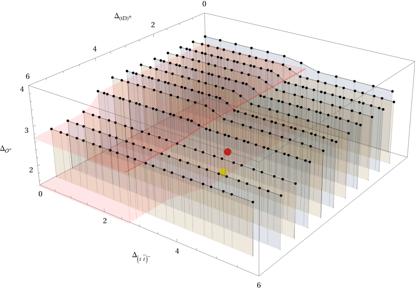
Refer to caption
Figure 5: Bounds on the dimension of the first 𝒮𝒮\mathcal{S}-parity even singlet 𝒪+superscript𝒪\mathcal{O}^{+} in the t×t¯𝑡¯𝑡t\times\bar{t} and the D×D¯D¯D\text{D}\times{\bar{\text{D}}} OPEs as a function of the scaling dimension of (tD)±superscript𝑡Dplus-or-minus{(t\text{D})}^{\pm} and (tt¯)superscript𝑡¯𝑡{(t\bar{t})}^{-}. The GFB solution, given in eq. (2.25), is shown in red. The ε𝜀\varepsilon-expansion results for the magnetic line defect are given in yellow. The light-shaded region represents the results for the agnostic bound Δ(tt¯)+=Δ(tt¯)subscriptΔsuperscript𝑡¯𝑡subscriptΔsuperscript𝑡¯𝑡\Delta_{{(t\bar{t})}^{+}}=\Delta_{{(t\bar{t})}^{-}}. Λ=33,P=63formulae-sequenceΛ33𝑃63\Lambda=33,P=63.

There are several operators one can study with these crossing equations. On the one hand, we have the leading non-identity 𝒮𝒮\mathcal{S}-parity even primary 𝒪+superscript𝒪\mathcal{O}^{+} which appears both in the t×t¯𝑡¯𝑡t\times\bar{t} and the D×D¯D¯D\text{D}\times{\bar{\text{D}}} OPEs. On the other hand, there are the leading 𝒮𝒮\mathcal{S}-parity odd primaries (tt¯)superscript𝑡¯𝑡{(t\bar{t})}^{-} and (DD¯)superscriptD¯D{(\text{D}\bar{\text{D}})}^{-}, which are in general different to each other. Finally, there is the lowest-lying O(2)F×SO(2)T𝑂subscript2𝐹𝑆𝑂subscript2𝑇O(2)_{F}\times SO(2)_{T} vector in the t×D𝑡Dt\times\text{D} channel

t×D(tD)±+,similar-to𝑡Dsuperscript𝑡Dplus-or-minus\displaystyle t\times\text{D}\sim{(t\text{D})}^{\pm}+\dots~{}, (4.4)

where the superscript ±plus-or-minus\pm denotes the 𝒮𝒮\mathcal{S} parity of the operator. In figure 5 we compute the upper bound on Δ𝒪+subscriptΔsuperscript𝒪\Delta_{\mathcal{O}^{+}}, while assuming gaps on the scaling dimensions of (tt¯)superscript𝑡¯𝑡{(t\bar{t})}^{-}, (tD)±superscript𝑡Dplus-or-minus{(t\text{D})}^{\pm} keeping Δ(tD)+=Δ(tD)subscriptΔsuperscript𝑡DsubscriptΔsuperscript𝑡D\Delta_{{(t\text{D})}^{+}}=\Delta_{{(t\text{D})}^{-}}. We take all other gaps to be very close to the unitarity bound, concretely we set them to Δ>0.001Δ0.001\Delta>0.001. If we are interested in the most ‘agnostic’ bound with Δ𝒪+=Δ(tt¯)subscriptΔsuperscript𝒪subscriptΔsuperscript𝑡¯𝑡\Delta_{\mathcal{O}^{+}}=\Delta_{{(t\bar{t})}^{-}}, then the allowed region shrinks to the light-red region of figure 5, which contains both the GFB (red dot) and the ε𝜀\varepsilon-expansion result for the magnetic line defect. The latter is far from saturating the upper bound and it seems hard to make progress without further assumptions. We will come back to this issue in section 4.3. The bounds are very uniform and show two drops, one in the Δ(tt¯)subscriptΔsuperscript𝑡¯𝑡\Delta_{{(t\bar{t})}^{-}} direction around Δ(tt¯)3similar-to-or-equalssubscriptΔsuperscript𝑡¯𝑡3\Delta_{{(t\bar{t})}^{-}}\simeq 3 and one in the Δ(tD)±subscriptΔsuperscript𝑡Dplus-or-minus\Delta_{{(t\text{D})}^{\pm}} direction around Δ(tD)±5similar-to-or-equalssubscriptΔsuperscript𝑡Dplus-or-minus5\Delta_{{(t\text{D})}^{\pm}}\simeq 5. For Δ(tD)±5greater-than-or-equivalent-tosubscriptΔsuperscript𝑡Dplus-or-minus5\Delta_{{(t\text{D})}^{\pm}}\gtrsim 5 the bound on Δ𝒪+subscriptΔsuperscript𝒪\Delta_{\mathcal{O}^{+}} becomes flat and approaches the value Δ𝒪+2.7similar-to-or-equalssubscriptΔsuperscript𝒪2.7\Delta_{\mathcal{O}^{+}}\simeq 2.7, a result we already found in the single-correlator bootstrap of the displacement operator of section 4.1.1. In the upper ‘cubic-shaped’ region we have that Δ𝒪+3.4less-than-or-similar-tosubscriptΔsuperscript𝒪3.4\Delta_{\mathcal{O}^{+}}\lesssim 3.4, which approaches the bound for a real GFF Δ𝒪+=3subscriptΔsuperscript𝒪3\Delta_{\mathcal{O}^{+}}=3.

Including one OPE coefficient.

In sections 4.1.1 and 4.1.2 we have seen that including one OPE coefficient leads to interesting bounds. We repeat this strategy here and bound (λtD(tD)+)2superscriptsubscript𝜆𝑡Dsuperscript𝑡D2(\lambda_{t\text{D}{(t\text{D})}^{+}})^{2} while varying the gap Δ(tD)±subscriptΔsuperscript𝑡Dplus-or-minus\Delta_{{(t\text{D})}^{\pm}} in the agnostic region Δ(tt¯)+=Δ(tt¯)subscriptΔsuperscript𝑡¯𝑡subscriptΔsuperscript𝑡¯𝑡\Delta_{{(t\bar{t})}^{+}}=\Delta_{{(t\bar{t})}^{-}}. It turns out that (λtD(tD)+)2superscriptsubscript𝜆𝑡Dsuperscript𝑡D2(\lambda_{t\text{D}{(t\text{D})}^{+}})^{2} is unbounded for Δ𝒪+2.7less-than-or-similar-tosubscriptΔsuperscript𝒪2.7\Delta_{\mathcal{O}^{+}}\lesssim 2.7. Above this value and for Δ𝒪+3.4less-than-or-similar-tosubscriptΔsuperscript𝒪3.4\Delta_{\mathcal{O}^{+}}\lesssim 3.4 there exists an upper bound which is shown in figure 6, while for Δ𝒪+3.4greater-than-or-equivalent-tosubscriptΔsuperscript𝒪3.4\Delta_{\mathcal{O}^{+}}\gtrsim 3.4 the upper bound (λtD(tD)+)2superscriptsubscript𝜆𝑡Dsuperscript𝑡D2(\lambda_{t\text{D}{(t\text{D})}^{+}})^{2} becomes negative, consistently with the results shown in figure 5. Since we are assuming a gap on the lowest operator Δ(tD)±subscriptΔsuperscript𝑡Dplus-or-minus\Delta_{{(t\text{D})}^{\pm}}, but do not make any assumptions on the scaling dimension of the next operator in the t×D𝑡Dt\times\text{D} OPE, the lower bound on (λtD(tD)+)2superscriptsubscript𝜆𝑡Dsuperscript𝑡D2(\lambda_{t\text{D}{(t\text{D})}^{+}})^{2} is at zero.

Refer to caption
Figure 6: Bounds on (λtD(tD)+)2superscriptsubscript𝜆𝑡Dsuperscript𝑡D2(\lambda_{t\text{D}{(t\text{D})}^{+}})^{2} as a function of the scaling dimension of Δ(tD)+subscriptΔsuperscript𝑡D\Delta_{{(t\text{D})}^{+}} and of the scaling dimension of the first parity-even singlet Δ𝒪+subscriptΔsuperscript𝒪\Delta_{\mathcal{O}^{+}}. The gap on the dimension Δ(tD)subscriptΔsuperscript𝑡D\Delta_{{(t\text{D})}^{-}} is set to Δ(tD)+subscriptΔsuperscript𝑡D\Delta_{{(t\text{D})}^{+}}, and all other gaps are set to 0.001. The GFB solution given in eq. (2.25) is marked by the red dot. Λ=33,P=63formulae-sequenceΛ33𝑃63\Lambda=33,P=63.

The ε=1𝜀1\varepsilon=1 solution of the ε𝜀\varepsilon-expansion for the magnetic line defect is not shown, since it lies far within the bounds in the region where the OPE coefficient (λtD(tD)+)2superscriptsubscript𝜆𝑡Dsuperscript𝑡D2(\lambda_{t\text{D}{(t\text{D})}^{+}})^{2} is unbounded.

4.2 Bootstrapping the monodromy line defect in the O(2)𝑂2O(2) model

The approach adopted so far was agnostic, in that we bounded CFT data without committing to any particular model. In this section we pursue a complementary approach, and combine the numerical bootstrap with the ε𝜀\varepsilon-expansion with the goal of bootstrapping the monodromy defect in the O(2)𝑂2O(2) model. Recall from section 3.1 two universal features of this monodromy defect: (i) for generic values of the parameter v[0,1)𝑣01v\in[0,1) the flavor symmetry of the model is SO(2)F𝑆𝑂subscript2𝐹SO(2)_{F}, which gets enhanced to O(2)F𝑂subscript2𝐹O(2)_{F} for v=0,12𝑣012v=0,\frac{1}{2}; (ii) the defect spectrum contains a family of 𝒮𝒮\mathcal{S}-parity even defect primaries ΨssubscriptΨ𝑠\Psi_{s} with SO(2)F𝑆𝑂subscript2𝐹SO(2)_{F} charge v𝑣v and transverse spin s+v𝑠𝑣s\in\mathbb{Z}+v. These two features can be combined in our numerical bootstrap problem as follows. First, we consider a system of correlation functions that involve the lowest-lying operator with SO(2)F𝑆𝑂subscript2𝐹SO(2)_{F} charge r=v𝑟𝑣r=v and its partner with charge r=1v𝑟1𝑣r=1-v. By charge conservation, the non-zero correlation functions are

Ψv(τ1)Ψ¯v(τ2)Ψv(τ3)Ψ¯v(τ4),Ψ1v(τ1)Ψ¯1v(τ2)Ψ1v(τ3)Ψ¯1v(τ4),Ψv(τ1)Ψ¯1v(τ2)Ψ1v(τ3)Ψ¯v(τ4),delimited-⟨⟩subscriptΨ𝑣subscript𝜏1subscript¯Ψ𝑣subscript𝜏2subscriptΨ𝑣subscript𝜏3subscript¯Ψ𝑣subscript𝜏4delimited-⟨⟩subscriptΨ1𝑣subscript𝜏1subscript¯Ψ1𝑣subscript𝜏2subscriptΨ1𝑣subscript𝜏3subscript¯Ψ1𝑣subscript𝜏4delimited-⟨⟩subscriptΨ𝑣subscript𝜏1subscript¯Ψ1𝑣subscript𝜏2subscriptΨ1𝑣subscript𝜏3subscript¯Ψ𝑣subscript𝜏4\displaystyle\begin{split}\langle\Psi_{v}(\tau_{1})\bar{\Psi}_{v}(\tau_{2})\Psi_{v}(\tau_{3})\bar{\Psi}_{v}(\tau_{4})\rangle\>,&\quad\langle\Psi_{1-v}(\tau_{1})\bar{\Psi}_{1-v}(\tau_{2})\Psi_{1-v}(\tau_{3})\bar{\Psi}_{1-v}(\tau_{4})\rangle\>,\\ \langle\Psi_{v}(\tau_{1})\bar{\Psi}_{1-v}&(\tau_{2})\Psi_{1-v}(\tau_{3})\bar{\Psi}_{v}(\tau_{4})\rangle\>,\end{split} (4.5)

which lead to the crossing equations presented in eq. (2.24). Although for general v𝑣v the monodromy defect is not invariant under O(2)F𝑂subscript2𝐹O(2)_{F} symmetry, but only under SO(2)F𝑆𝑂subscript2𝐹SO(2)_{F} symmetry, we can use the same crossing equations in both cases. The justification for this appeared in [52], but we repeat it here for convenience. The tensor ϵijsubscriptitalic-ϵ𝑖𝑗\epsilon_{ij} is invariant under SO(2)𝑆𝑂2SO(2) but not under O(2)𝑂2O(2), so the antisymmetric representation is isomorphic to the singlet representation for SO(2)𝑆𝑂2SO(2) but not for O(2)𝑂2O(2). However, this does not lead to additional relations in the crossing equations, because even when the singlet and antisymmetric representations are isomorphic, we can distinguish them since they contain 𝒮𝒮{\mathcal{S}}-parity even and odd operators respectively.
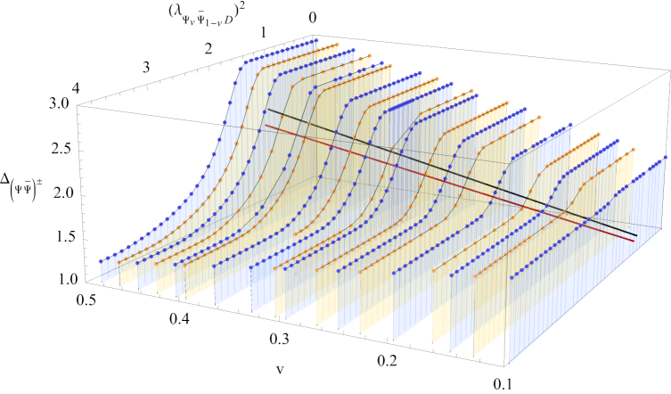
Refer to caption
(a)
Refer to caption
(b)
Figure 7: Bounds on the dimension of the first singlet in the Ψs×Ψ¯ssubscriptΨ𝑠subscript¯Ψ𝑠\Psi_{s}\times\bar{\Psi}_{s} OPE Δ(ΨΨ¯)±subscriptΔsuperscriptΨ¯Ψplus-or-minus\Delta_{{(\Psi\bar{\Psi})}^{\pm}} versus the OPE coefficient of the displacement operator and the monodromy v𝑣v. The gaps on the dimension of the lowest-lying operators in all other channels is set to the unitarity bound. Parity-even and odd operators are set to have the same gaps. The gray line corresponds to the ε𝜀\varepsilon-expansion results. Λ=21,P=41formulae-sequenceΛ21𝑃41\Lambda=21,P=41.

Second, we input the scaling dimensions of ΨssubscriptΨ𝑠\Psi_{s} using the predictions from the ε𝜀\varepsilon-expansion in eq. (3.7), extrapolated to ε=1𝜀1\varepsilon=1. With this input, we put an upper bound to the dimension of the lowest-lying operator in Ψs×Ψ¯ssubscriptΨ𝑠subscript¯Ψ𝑠\Psi_{s}\times\bar{\Psi}_{s}, i.e.

Ψs×Ψ¯s=𝟙+(ΨΨ¯)±+,s=v, or v1.formulae-sequencesubscriptΨ𝑠subscript¯Ψ𝑠1superscriptΨ¯Ψplus-or-minus𝑠𝑣 or 𝑣1\displaystyle\Psi_{s}\times\bar{\Psi}_{s}={\mathds{1}}+{(\Psi\bar{\Psi})}^{\pm}+\dots,\quad s=v,\text{~{}or~{}}v-1~{}. (4.6)

Note that (ΨΨ¯)±superscriptΨ¯Ψplus-or-minus{(\Psi\bar{\Psi})}^{\pm} is a singlet under SO(2)T×SO(2)F𝑆𝑂subscript2𝑇𝑆𝑂subscript2𝐹SO(2)_{T}\times SO(2)_{F}, and it could be either 𝒮𝒮\mathcal{S}-parity even or 𝒮𝒮\mathcal{S}-parity odd. For the Ψv×Ψ¯v1subscriptΨ𝑣subscript¯Ψ𝑣1\Psi_{v}\times\bar{\Psi}_{v-1} OPE we assume the lowest-lying operator is the displacement operator, which is 𝒮𝒮\mathcal{S}-parity even. We will further assume that there is no operator in the 𝒮𝒮\mathcal{S}-parity odd channel with dimension smaller than the displacement, namely:

(Ψv×Ψ¯v1)+=D+,(Ψv×Ψ¯v1)=(ΨvΨ¯v1)+,Δ(ΨvΨ¯v1)2.formulae-sequencesuperscriptsubscriptΨ𝑣subscript¯Ψ𝑣1Dformulae-sequencesuperscriptsubscriptΨ𝑣subscript¯Ψ𝑣1superscriptsubscriptΨ𝑣subscript¯Ψ𝑣1subscriptΔsuperscriptsubscriptΨ𝑣subscript¯Ψ𝑣12\displaystyle(\Psi_{v}\times\bar{\Psi}_{v-1})^{+}=\text{D}+\dots\>,\quad(\Psi_{v}\times\bar{\Psi}_{v-1})^{-}=(\Psi_{v}\bar{\Psi}_{v-1})^{-}+\dots\>,\quad\Delta_{(\Psi_{v}\bar{\Psi}_{v-1})^{-}}\geq 2~{}. (4.7)

These assumptions are true in the ε𝜀\varepsilon-expansion, where one can see at leading order that the displacement operator appears in the OPE with the expected dimension ΔD=2subscriptΔD2\Delta_{\text{D}}=2, see appendix A for more details.

In figure 7 we plot the upper bound on Δ(ΨΨ¯)±subscriptΔsuperscriptΨ¯Ψplus-or-minus\Delta_{{(\Psi\bar{\Psi})}^{\pm}} as a function of the SO(2)F𝑆𝑂subscript2𝐹SO(2)_{F} charge v𝑣v and the OPE coefficient of the displacement operator (λΨvΨ¯1vD)2superscriptsubscript𝜆subscriptΨ𝑣subscript¯Ψ1𝑣D2(\lambda_{\Psi_{v}\bar{\Psi}_{1-v}\text{D}})^{2}. Let us stress that v𝑣v enters the crossing equations through the dimension of the external operators, which we take to be the ε𝜀\varepsilon-expansion prediction (3.7). Furthermore, since the crossing equations in eq. (4.5) are invariant under v1v𝑣1𝑣v\leftrightarrow 1-v, it suffices to consider the range 0<v1/20𝑣120<v\leq 1/2, where the limiting case v=1/2𝑣12v=1/2 corresponds to the 2subscript2\mathbb{Z}_{2} twist defect studied in [25]. In the figure we observe a family of drops as we move along the (λΨvΨ¯1vD)2\lambda_{\Psi_{v}\bar{\Psi}_{1-v}\text{D}})^{2} direction, and as we increase v𝑣v towards v=1/2𝑣12v=1/2 these drops become sharper and move slightly to the right. It is promising that the ε𝜀\varepsilon-expansion results are above and left of the free theory solutions, because this makes it possible for the theoretical prediction to saturate the bound. However, for the results with Λ=21Λ21\Lambda=21 derivatives shown in figure 7(b), both the ε𝜀\varepsilon-expansion result and the free theory solution are still somewhat far from saturating the numerical bound.

One possibility that we explore in figure 8 is whether increasing the number of derivatives can bring the bound closer to the analytical prediction. For concreteness we focus on v=1/3𝑣13v=1/3,141414The choice v=1/3𝑣13v=1/3 is particularly interesting for its connection to half-BPS defects in superconformal field theories. For example, we expect that the monodromy defect for the Wess-Zumino model [59] preserves supersymmetry whenever v=1/3𝑣13v=1/3. and we increase the number of derivatives to Λ=33Λ33\Lambda=33. We observe that the kink moves slightly towards the left of the plot, but remains somewhat far from the analytical prediction. Another possibility is that one needs to consider less agnostic gap assumptions in the channels besides Ψv×Ψ¯1vsubscriptΨ𝑣subscript¯Ψ1𝑣\Psi_{v}\times\bar{\Psi}_{1-v}, or perhaps higher-order corrections from the ε𝜀\varepsilon-expansion are needed to reconcile theory and numerics. In either case, this provides a good motivation for a more detailed study of monodromy defects using the ε𝜀\varepsilon-expansion, to which we hope to come back in future work.
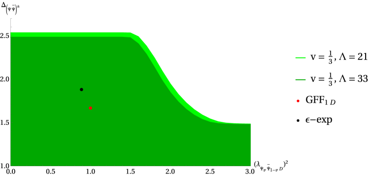
Refer to caption
Figure 8: Bounds on the dimension of the first singlet in the Ψs×Ψ¯ssubscriptΨ𝑠subscript¯Ψ𝑠\Psi_{s}\times\bar{\Psi}_{s} OPE Δ(ΨΨ¯)±subscriptΔsuperscriptΨ¯Ψplus-or-minus\Delta_{{(\Psi\bar{\Psi})}^{\pm}} versus the OPE coefficient of the displacement operator (λΨvΨ¯1vD)2superscriptsubscript𝜆subscriptΨ𝑣subscript¯Ψ1𝑣𝐷2(\lambda_{\Psi_{v}\bar{\Psi}_{1-v}D})^{2}. v=13𝑣13v=\frac{1}{3} and the gaps on the dimension of the lowest-lying operators in all other channels are set to the unitarity bound. Parity-even and odd operators are set to have the same gaps. Λ=21,P=41formulae-sequenceΛ21𝑃41\Lambda=21,P=41 and Λ=33,P=53formulae-sequenceΛ33𝑃53\Lambda=33,P=53.

4.3 Bootstrapping the localized magnetic field line defect

This section studies the magnetic line defect of [5] in the bulk O(3)𝑂3O(3) CFT, combining the numerical bootstrap with the ε𝜀\varepsilon-expansion results of section 3.2. There are two features of the magnetic line defect which are important in our analysis: (i) the model is invariant under a O(2)FO(3)𝑂subscript2𝐹𝑂3O(2)_{F}\subset O(3) flavor symmetry and, (ii) the defect spectrum features a tilt operator t𝑡t transforming in the vector representation of O(2)F𝑂subscript2𝐹O(2)_{F}. To exploit these features, we consider a bootstrap problem involving the tilt t𝑡t and the lowest-dimension neutral scalar ϕ1subscriptitalic-ϕ1\phi_{1}, so we consider the correlation functions

ϕ1(τ1)ϕ1(τ2)ϕ1(τ3)ϕ1(τ4),delimited-⟨⟩subscriptitalic-ϕ1subscript𝜏1subscriptitalic-ϕ1subscript𝜏2subscriptitalic-ϕ1subscript𝜏3subscriptitalic-ϕ1subscript𝜏4\displaystyle\langle\phi_{1}(\tau_{1})\phi_{1}(\tau_{2})\phi_{1}(\tau_{3})\phi_{1}(\tau_{4})\rangle~{}\>, t(τ1)t¯(τ2)t(τ3)t¯(τ4),delimited-⟨⟩𝑡subscript𝜏1¯𝑡subscript𝜏2𝑡subscript𝜏3¯𝑡subscript𝜏4\displaystyle\quad\langle t(\tau_{1})\bar{t}(\tau_{2})t(\tau_{3})\bar{t}(\tau_{4})\rangle~{}\>,
ϕ1(τ1)ϕ1(τ2)\displaystyle\langle\phi_{1}(\tau_{1})\phi_{1}(\tau_{2}) t(τ3)t¯(τ4),\displaystyle t(\tau_{3})\bar{t}(\tau_{4})\rangle~{}\>, (4.8)

plus all other non-equivalent orderings. The corresponding crossing equations are given in eq. (2.23).151515Since we are not including the displacement operator, this system of correlation functions is agnostic about the co-dimension of the line defect. It will enter only implicitly via our gap assumptions which are determined by the ε𝜀\varepsilon-expansion results of section 3.2. The inclusion of the displacement operator is more involved. Nevertheless, it is an interesting extension and we will leave it for future work. There are five OPE channels that enter in our discussion

ϕ1×ϕ1𝟙+ϕ1+s+,(t×t¯)+𝟙+ϕ1+s+,(t×t¯)A+,t×tT+,t×ϕ1t+V+,\displaystyle\begin{split}&\phi_{1}\times\phi_{1}\sim{\mathds{1}}+\phi_{1}+s_{-}+\cdots\>,\quad(t\times\bar{t})^{+}\sim{\mathds{1}}+\phi_{1}+s_{-}+\cdots\>,\quad\\ &(t\times\bar{t})^{-}\sim A+\cdots,\quad t\times t\sim T+\dots\>,\quad t\times\phi_{1}\sim t+V+\cdots\>,\end{split} (4.9)

where further details on the operators exchanged can be found in section 3.2.1. Note that the external operators are exchanged in some of the fusion channels, which allows us to impose the extra relations λϕ1tt¯=λtt¯ϕ1subscript𝜆subscriptitalic-ϕ1𝑡¯𝑡subscript𝜆𝑡¯𝑡subscriptitalic-ϕ1\lambda_{\phi_{1}t\bar{t}}=\lambda_{t\bar{t}\phi_{1}} in the crossing equations. Furthermore, we impose the following gaps

Δs=2.36,ΔA=3,ΔT=2.18,ΔV=3.18,formulae-sequencesubscriptΔsubscript𝑠2.36formulae-sequencesubscriptΔ𝐴3formulae-sequencesubscriptΔ𝑇2.18subscriptΔ𝑉3.18\displaystyle\Delta_{s_{-}}=2.36\>,\qquad\Delta_{A}=3\>,\qquad\Delta_{T}=2.18\>,\qquad\Delta_{V}=3.18\>, (4.10)

where the values are the O(ε)𝑂𝜀O(\varepsilon) results for the scaling dimensions from eqs. (3.15), (3.16) and (3.17). With these assumptions we bound the scaling dimensions of ϕ1subscriptitalic-ϕ1\phi_{1} and t𝑡t. Although we could also fix the scaling dimensions of t𝑡t and ϕ1subscriptitalic-ϕ1\phi_{1} using the perturbative calculation (in particular, t𝑡t has protected dimension Δt=1subscriptΔ𝑡1\Delta_{t}=1), we keep them unfixed to see how they are constrained by the numerics. This logic is inspired by the search for the Ising model island, where (physically motivated) gap assumptions led to constraints on the external operators σ𝜎\sigma and ϵitalic-ϵ\epsilon [46]. Our results are presented in figure 9, where the allowed values in the (Δt,Δϕ1)subscriptΔ𝑡subscriptΔsubscriptitalic-ϕ1(\Delta_{t},\Delta_{\phi_{1}}) plane are shown in green.

Refer to caption
(a)
Refer to caption
(b)
Figure 9: Bootstrapping the O(3)𝑂3O(3)-breaking line defect. In (a), bounds on the scaling dimensions Δϕ1subscriptΔsubscriptitalic-ϕ1\Delta_{\phi_{1}} and ΔtsubscriptΔ𝑡\Delta_{t} for Λ=21,P=41formulae-sequenceΛ21𝑃41\Lambda=21,P=41. The gaps are given in eq. (4.10). Allowed values of (Δt,Δϕ1)subscriptΔ𝑡subscriptΔsubscriptitalic-ϕ1(\Delta_{t},\Delta_{\phi_{1}}) are given in green. In (b), the bound on Δϕ1subscriptΔsubscriptitalic-ϕ1\Delta_{\phi_{1}} for Δt=1subscriptΔ𝑡1\Delta_{t}=1 as a function of the number of derivatives ΛΛ\Lambda, for which a fit is performed.

The lower bound for t𝑡t is strikingly close to 1, the numerics seems to be rediscovering the tilt. For this value of ΔtsubscriptΔ𝑡\Delta_{t}, the bound goes up and cuts out a corner. It should also be noted that there are numerical instabilities in the region with large Δϕ1subscriptΔsubscriptitalic-ϕ1\Delta_{\phi_{1}} outside the range of figure 9(a). The lower bound on Δϕ1subscriptΔsubscriptitalic-ϕ1\Delta_{\phi_{1}} is on the other hand weaker, its value being nowhere close to the Padé extrapolation of Δϕ11.55similar-to-or-equalssubscriptΔsubscriptitalic-ϕ11.55\Delta_{\phi_{1}}\simeq 1.55 (and it is even further away from the crude ε𝜀\varepsilon-expansion result Δϕ1=2+O(ε2)subscriptΔsubscriptitalic-ϕ12𝑂superscript𝜀2\Delta_{\phi_{1}}=2+O(\varepsilon^{2})). It is nevertheless a non-trivial numerical result that such a lower bound exists at all. Note that the magnetic line defect has no relevant operators [5], so Δϕ1>1subscriptΔsubscriptitalic-ϕ11\Delta_{\phi_{1}}>1 should be expected. Our O(ε)𝑂𝜀O(\varepsilon) assumptions allow for a weaker numerical bound on Δϕ1subscriptΔsubscriptitalic-ϕ1\Delta_{\phi_{1}}. For the physically interesting value Δt=1subscriptΔ𝑡1\Delta_{t}=1, figure 9(b) displays an extrapolation to infinite number of derivatives of the lower bound, which converges to

Δϕ10.76.greater-than-or-equivalent-tosubscriptΔsubscriptitalic-ϕ10.76\Delta_{\phi_{1}}\gtrsim 0.76\,. (4.11)

Again, we cannot completely rule out the region with Δϕ11subscriptΔsubscriptitalic-ϕ11\Delta_{\phi_{1}}\leq 1. It could be that our numerics is not strong enough to rule out the presence of relevant operators, so we should either change our assumptions or include more external operators to the system of eq. (4.3). Another possibility which we cannot rule out is the existence of alternative models consistent with our assumptions but with one relevant scalar in the spectrum. Definitely, we think this result calls for a more systematic investigation, which nowadays can be efficiently performed with the help of the Navigator Function [60, 61] in order to search for bootstrap islands in a large parameter space. Finally, one may wonder if our gap assumptions allow for upper bounds on Δϕ1subscriptΔsubscriptitalic-ϕ1\Delta_{\phi_{1}} as well. Clearly, Δϕ1subscriptΔsubscriptitalic-ϕ1\Delta_{\phi_{1}} cannot be bigger than 2.36similar-to-or-equalsabsent2.36\simeq 2.36, which is when the next operator ΔssubscriptΔsubscript𝑠\Delta_{s_{-}} appears, see eq. (4.10). Below this threshold there seems to be no upper bound, at least with the current number of derivatives.

Bounds on OPE coefficients.
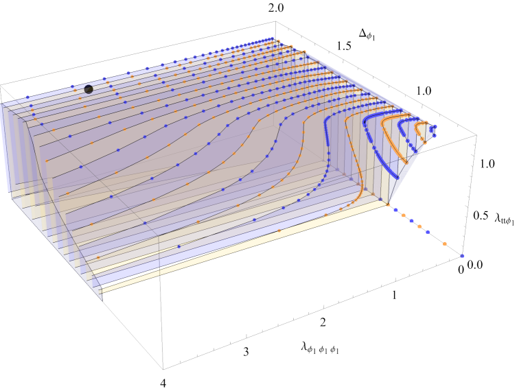
Refer to caption
Figure 10: Bounds on the OPE coefficients λtt¯ϕ1subscript𝜆𝑡¯𝑡subscriptitalic-ϕ1\lambda_{t\bar{t}\phi_{1}} and λϕ1ϕ1ϕ1subscript𝜆subscriptitalic-ϕ1subscriptitalic-ϕ1subscriptitalic-ϕ1\lambda_{\phi_{1}\phi_{1}\phi_{1}} as a function of the gap Δϕ1subscriptΔsubscriptitalic-ϕ1\Delta_{\phi_{1}} for the O(3)𝑂3O(3)-breaking magnetic line defect. The black dot is the prediction from the ε𝜀\varepsilon-expansion. The gaps are given in eq. (4.10). Λ=21,P=41formulae-sequenceΛ21𝑃41\Lambda=21,P=41.

Having constrained the region (Δϕ1,Δt)subscriptΔsubscriptitalic-ϕ1subscriptΔ𝑡(\Delta_{\phi_{1}},\Delta_{t}), we now set ΔtsubscriptΔ𝑡\Delta_{t} to its physical value of 1, but continue to treat Δϕ1subscriptΔsubscriptitalic-ϕ1\Delta_{\phi_{1}} as an external parameter. The goal is to bound the OPE coefficients (λtt¯ϕ1)2superscriptsubscript𝜆𝑡¯𝑡subscriptitalic-ϕ12(\lambda_{t\bar{t}\phi_{1}})^{2} and (λϕ1ϕ1ϕ1)2superscriptsubscript𝜆subscriptitalic-ϕ1subscriptitalic-ϕ1subscriptitalic-ϕ12(\lambda_{\phi_{1}\phi_{1}\phi_{1}})^{2} as functions of Δϕ1subscriptΔsubscriptitalic-ϕ1\Delta_{\phi_{1}}, which in turn were computed in the ε𝜀\varepsilon-expansion in section 3.2, see eqs. (3.14) and (3.50). To this end, we employ the strategy developed in [46], i.e. we introduce the OPE angle θ𝜃\theta defined as

tanθ=λϕ1ϕ1ϕ1λtt¯ϕ1,𝜃subscript𝜆subscriptitalic-ϕ1subscriptitalic-ϕ1subscriptitalic-ϕ1subscript𝜆𝑡¯𝑡subscriptitalic-ϕ1\tan\theta=\frac{\lambda_{\phi_{1}\phi_{1}\phi_{1}}}{\lambda_{t\bar{t}\phi_{1}}}\>, (4.12)

and we search for upper and lower bounds on the quantity (λϕ1ϕ1ϕ1)2+(λtt¯ϕ1)2superscriptsubscript𝜆subscriptitalic-ϕ1subscriptitalic-ϕ1subscriptitalic-ϕ12superscriptsubscript𝜆𝑡¯𝑡subscriptitalic-ϕ12(\lambda_{\phi_{1}\phi_{1}\phi_{1}})^{2}+(\lambda_{t\bar{t}\phi_{1}})^{2} as a function of θ[0,π)𝜃0𝜋\theta\in[0,\pi) and of Δϕ1subscriptΔsubscriptitalic-ϕ1\Delta_{\phi_{1}}. For concreteness we restrict to the case where 0θ<π20𝜃𝜋20\leq\theta<\frac{\pi}{2} (i.e. λϕ1ϕ1ϕ1λtt¯ϕ10subscript𝜆subscriptitalic-ϕ1subscriptitalic-ϕ1subscriptitalic-ϕ1subscript𝜆𝑡¯𝑡subscriptitalic-ϕ10\lambda_{\phi_{1}\phi_{1}\phi_{1}}\lambda_{t\bar{t}\phi_{1}}\geq 0), which is also compatible with the leading ε𝜀\varepsilon-expansion prediction. The numerics is of course sensitive to the relative sign only. The results in figure 10 show that for any value of the OPE coefficients λϕ1ϕ1ϕ1subscript𝜆subscriptitalic-ϕ1subscriptitalic-ϕ1subscriptitalic-ϕ1\lambda_{\phi_{1}\phi_{1}\phi_{1}} and λtt¯ϕ1subscript𝜆𝑡¯𝑡subscriptitalic-ϕ1\lambda_{t\bar{t}\phi_{1}}, there is an excluded region which is fully consistent with the lower bound from figure 9(a). However, as it turns out, for λϕ1ϕ1ϕ1/λtt¯ϕ10subscript𝜆subscriptitalic-ϕ1subscriptitalic-ϕ1subscriptitalic-ϕ1subscript𝜆𝑡¯𝑡subscriptitalic-ϕ10\lambda_{\phi_{1}\phi_{1}\phi_{1}}/\lambda_{t\bar{t}\phi_{1}}\geq 0, the excluded region is larger and exists for Δϕ10.9less-than-or-similar-tosubscriptΔsubscriptitalic-ϕ10.9\Delta_{\phi_{1}}\lesssim 0.9, while for λϕ1ϕ1ϕ1/λtt¯ϕ10subscript𝜆subscriptitalic-ϕ1subscriptitalic-ϕ1subscriptitalic-ϕ1subscript𝜆𝑡¯𝑡subscriptitalic-ϕ10\lambda_{\phi_{1}\phi_{1}\phi_{1}}/\lambda_{t\bar{t}\phi_{1}}\leq 0, only values up to Δϕ10.7less-than-or-similar-tosubscriptΔsubscriptitalic-ϕ10.7\Delta_{\phi_{1}}\lesssim 0.7 are excluded. For values between 0.7Δϕ11.1less-than-or-similar-to0.7subscriptΔsubscriptitalic-ϕ1less-than-or-similar-to1.10.7\lesssim\Delta_{\phi_{1}}\lesssim 1.1, the upper and lower bounds on λtt¯ϕ1subscript𝜆𝑡¯𝑡subscriptitalic-ϕ1\lambda_{t\bar{t}\phi_{1}} approach each other until they meet, after which the upper bound goes to zero. This means that certain values of the OPE coefficent λϕ1ϕ1ϕ1subscript𝜆subscriptitalic-ϕ1subscriptitalic-ϕ1subscriptitalic-ϕ1\lambda_{\phi_{1}\phi_{1}\phi_{1}} are ruled out by the numerical bootstrap, even though the corresponding Δϕ1subscriptΔsubscriptitalic-ϕ1\Delta_{\phi_{1}} values are allowed in figure 9(a). For Δϕ11.1greater-than-or-equivalent-tosubscriptΔsubscriptitalic-ϕ11.1\Delta_{\phi_{1}}\gtrsim 1.1, the bound on λtt¯ϕ1subscript𝜆𝑡¯𝑡subscriptitalic-ϕ1\lambda_{t\bar{t}\phi_{1}} is always positive. There is an intriguing feature visible starting around Δϕ10.9less-than-or-similar-tosubscriptΔsubscriptitalic-ϕ10.9\Delta_{\phi_{1}}\lesssim 0.9 and continuing until Δϕ11.4similar-to-or-equalssubscriptΔsubscriptitalic-ϕ11.4\Delta_{\phi_{1}}\simeq 1.4, where the projection onto the (λϕ1ϕ1ϕ1,λtt¯ϕ1)subscript𝜆subscriptitalic-ϕ1subscriptitalic-ϕ1subscriptitalic-ϕ1subscript𝜆𝑡¯𝑡subscriptitalic-ϕ1(\lambda_{\phi_{1}\phi_{1}\phi_{1}},\lambda_{t\bar{t}\phi_{1}}) plane shows a pronunced cusp, see figure 11(a). For higher values of Δϕ1subscriptΔsubscriptitalic-ϕ1\Delta_{\phi_{1}} this feature disappears and the plot becomes smooth. For the quadrant where the OPE coefficients have opposite sign this cusp is not present. In order to better understand this feature, we have plotted two slices of the three-dimensional plot in figure 11.
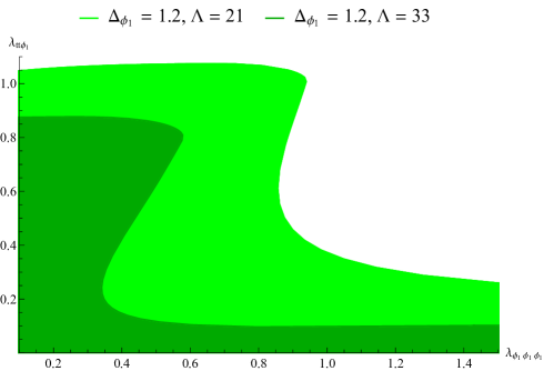
Refer to caption
(a)
Refer to caption
(b)
Figure 11: Bootstrapping the O(3)𝑂3O(3)-breaking magnetic line defect. Upper bounds on the OPE coefficient λϕ1ϕ1ϕ1subscript𝜆subscriptitalic-ϕ1subscriptitalic-ϕ1subscriptitalic-ϕ1\lambda_{\phi_{1}\phi_{1}\phi_{1}} as a function of λtt¯ϕ1subscript𝜆𝑡¯𝑡subscriptitalic-ϕ1\lambda_{t\bar{t}\phi_{1}}. Λ=21,P=41formulae-sequenceΛ21𝑃41\Lambda=21,P=41 and Λ=33,P=63formulae-sequenceΛ33𝑃63\Lambda=33,P=63. In (a) the external scalar has dimension Δϕ1=1.2subscriptΔsubscriptitalic-ϕ11.2\Delta_{\phi_{1}}=1.2. In (b) the external scalar has dimension Δϕ1=1.55subscriptΔsubscriptitalic-ϕ11.55\Delta_{\phi_{1}}=1.55. The ε𝜀\varepsilon-expansion result is shown by the black dot.

For figure 11(a) we have chosen the value Δϕ1=1.2subscriptΔsubscriptitalic-ϕ11.2\Delta_{\phi_{1}}=1.2 somewhat arbitrarily, in order to highlight a region where the cusp is clearly visible. It appears around λϕ1ϕ1ϕ10.9similar-to-or-equalssubscript𝜆subscriptitalic-ϕ1subscriptitalic-ϕ1subscriptitalic-ϕ10.9\lambda_{\phi_{1}\phi_{1}\phi_{1}}\simeq 0.9, although its position shifts depending on the value of Δϕ1subscriptΔsubscriptitalic-ϕ1\Delta_{\phi_{1}} and the number of derivatives. In figure 11(b) we have chosen Δϕ1=1.55subscriptΔsubscriptitalic-ϕ11.55\Delta_{\phi_{1}}=1.55, which corresponds to the best estimate of the conformal dimension of ϕ1subscriptitalic-ϕ1\phi_{1} using a Padé approximation [5]. For this value of Δϕ1subscriptΔsubscriptitalic-ϕ1\Delta_{\phi_{1}} the features from figure 11(a) are gone and the bound is smooth. We have added in figure 11(b) the prediction coming from the ε𝜀\varepsilon-expansion for reference. We should warn the reader that this prediction is valid up to O(ε)𝑂𝜀O(\varepsilon), for which Δϕ1=2subscriptΔsubscriptitalic-ϕ12\Delta_{\phi_{1}}=2. Our numerical plot was obtained with a different set of assumptions, in particular for Δϕ1=1.55subscriptΔsubscriptitalic-ϕ11.55\Delta_{\phi_{1}}=1.55, which explains why the dot is outside the numerical exclusion region. One possibility is that the cusp is also present for Δϕ11.55similar-to-or-equalssubscriptΔsubscriptitalic-ϕ11.55\Delta_{\phi_{1}}\simeq 1.55, but was lost due to numerical precision. Indeed from figure 11(a) the feature becomes more pronounced when we jump from Λ=21Λ21\Lambda=21 to Λ=33Λ33\Lambda=33 derivatives. It would be remarkable if the numerics could be pushed, such that figure 11(b) starts looking more like figure 11(a). The position of the cusp would then be a good candidate for the magnetic line defect.

5 Conclusions and future directions

In this paper we have studied O(2)𝑂2O(2) line defects in a 3d bulk CFT with SO(2)𝑆𝑂2SO(2) flavor symmetry – the monodromy defect – or O(3)𝑂3O(3) flavor symmetry – the magnetic line defect – using the conformal bootstrap. After writing the corresponding crossing equations we applied the numerical machinery in order to obtain exclusion bounds valid for generic 1d defect CFTs. We concentrated mostly on two canonical operators: the displacement and the tilt. The displacement operator is truly universal in that it controls the breaking of translations due to the presence of the conformal defect. The tilt operator can exist when a conformal defect breaks a bulk global symmetry, which is still quite a generic phenomenon.

After obtaining general bounds that constrain the landscape of 1d theories, we changed gears and focused on two models of interest: the monodromy defect studied in [38, 39, 40], and the magnetic line defect described in [5]. In order to guide the numerics we complemented our bootstrap analysis with explicit analytic calculations in the ε𝜀\varepsilon-expansion. For the monodromy defect, the results had already appeared in [38, 39], while for the magnetic line defect most of the calculations presented in section 3.2 are new.

For the monodromy defect we have kept the gap assumptions to a minimum, using the dimension of the external operators from the ε𝜀\varepsilon-expansion results and imposing the existence of the displacement operator. Hence the numerical results are quite general, and they are fully consistent with the analytical data. The results for the magnetic line defect are more constraining. By imposing gaps coming from the ε𝜀\varepsilon-expansion, the allowed region for certain OPE coefficients shows a series of intriguing cusps. The location of these cusps however, does not match the best numerical estimates of the conformal dimension of the scalar field Δϕ11.55similar-to-or-equalssubscriptΔsubscriptitalic-ϕ11.55\Delta_{\phi_{1}}\simeq 1.55. Nevertheless, we consider this result an encouraging sign. Ways in which our methods can be improved include higher order terms in the ε𝜀\varepsilon-expansion, and higher precision in the numerics. The hope is that with these improvements, the region where the magnetic line defected is expected to sit also develops a cusp.

There are several avenues in which our research can be extended. A natural question to ask is whether one could construct a monodromy defect that breaks a bulk O(3)𝑂3O(3) symmetry to an O(2)𝑂2O(2) symmetry on the line. Such a defect would have a tilt operator, a displacement, and fundamental fields with transverse spin related to the charge of the monodromy. Mixed correlators with three external operators have already been studied in [62, 63, 64] in the context of O(2)𝑂2O(2) and O(3)𝑂3O(3) models.

Another interesting possibilty is to reproduce the ε𝜀\varepsilon-expansion results using purely bootstrap means, without explicit Feynman diagram calculations. This line of thinking has been particularly succesful, with numerous analytical results obtained using only symmetry arguments and basic structural constraints. A promising framework tailored for our setup is that of analytic functionals, which were used in [36] to study the Ising twist line defect with 2subscript2\mathbb{Z}_{2} global symmetry.

Furthermore, we could extend our results to line defects with O(N)𝑂𝑁O(N) flavor symmetry. In addition to the analytical tools used in this work, we would gain access to the large N𝑁N expansion, giving us perturbative results in a different regime to compare with the numerics. At the same time, these line defects could break a bulk O(N+m)𝑂𝑁𝑚O(N+m) symmetry to a defect O(N)𝑂𝑁O(N) symmetry, where N,m𝑁𝑚N,m\in\mathbb{Z}. In this generalization, the tilt will no longer be a vector under O(2)𝑂2O(2) flavour symmetry, but will be part of another representation.

Finally, our setup can generalized to study monodromy line defects in superconformal models, like the monodromy defect of the Wess-Zumino model studied in [59]. This model contains a displacement as well as a tilt operator due to the breaking of the R𝑅R-symmetry to a U(1)𝑈1U(1) symmetry on the defect, which in turn sit inside protected multiplets of the superconformal algebra. It would be interesting to pursue a systematic study of this setup using the superconformal bootstrap and we leave it for the future [65].

Acknowledgements

We would like to thank A. Antunes, N. Bobev, I. Burić, G. Cuomo, A. Kaviraj, D. Mazáč, J. Rong, V. Schomerus, E. Trevisani and B. van Rees for discussions. Also, we would like to thank the organizers of the conference ‘Bootstrap 2022’ for providing a place for fruitful discussions. EL would like to thank A. Antunes and B. van Rees for their collaboration and discussions on related projects. EL is supported by the Simons Foundation grant ##\#488659 (Simons Collaboration on the non-perturbative bootstrap). AG , PL and PvV acknowledge support from the DFG through the Emmy Noether research group ‘The Conformal Bootstrap Program’ project number 400570283, and through the German-Israeli Project Cooperation (DIP) grant ‘Holography and the Swampland’.

Appendix A More data on the O(N)𝑂𝑁O(N) monodromy defect in 3d

In this appendix, we give a more detailed explanation of the calculation of the dimensions and OPE coefficients given in section 3.1 and computed in [39].

A.1 OPE coefficients with the displacement operator

The displacement operator appears in the OPE of two defect modes Ψv×Ψ¯v1D+similar-tosubscriptΨ𝑣subscript¯Ψ𝑣1D\Psi_{v}\times\bar{\Psi}_{v-1}\sim\text{D}+\cdots. Hence, we are interested in the correlators involving these defect modes, which are

Ψv(x1)Ψ¯v(x2)Ψv(x3)Ψ¯v(x4),Ψ1v(x1)Ψ¯1v(x2)Ψ1v(x3)Ψ¯1v(x4),Ψv(x1)Ψ¯1v(x2)Ψ1v(x3)Ψ¯v(x4).delimited-⟨⟩subscriptΨ𝑣subscript𝑥1subscript¯Ψ𝑣subscript𝑥2subscriptΨ𝑣subscript𝑥3subscript¯Ψ𝑣subscript𝑥4delimited-⟨⟩subscriptΨ1𝑣subscript𝑥1subscript¯Ψ1𝑣subscript𝑥2subscriptΨ1𝑣subscript𝑥3subscript¯Ψ1𝑣subscript𝑥4delimited-⟨⟩subscriptΨ𝑣subscript𝑥1subscript¯Ψ1𝑣subscript𝑥2subscriptΨ1𝑣subscript𝑥3subscript¯Ψ𝑣subscript𝑥4\displaystyle\begin{split}\langle\Psi_{v}(\vec{x}_{1})\bar{\Psi}_{v}(\vec{x}_{2})\Psi_{v}(\vec{x}_{3})\bar{\Psi}_{v}(\vec{x}_{4})\rangle\>,&\quad\langle\Psi_{1-v}(\vec{x}_{1})\bar{\Psi}_{1-v}(\vec{x}_{2})\Psi_{1-v}(\vec{x}_{3})\bar{\Psi}_{1-v}(\vec{x}_{4})\rangle\>,\\ \langle\Psi_{v}(\vec{x}_{1})\bar{\Psi}_{1-v}&(\vec{x}_{2})\Psi_{1-v}(\vec{x}_{3})\bar{\Psi}_{v}(\vec{x}_{4})\rangle\>.\end{split} (A.1)

The results for the single-operator correlators were already computed in [25] for a 2subscript2\mathbb{Z}_{2} monodromy defect. For correlators with two operators Ψ1subscriptΨ1\Psi_{1} and Ψ2subscriptΨ2\Psi_{2}, the anomalous dimensions of the operators appearing in the OPEs are computed in [39], and from their results also the OPE coefficients can be readily derived.161616Note that our conventions differ slightly from those used in [39]; in particular, we normalize the two-point function as Ψ¯s1(x1)Ψs2(x2)0=δs1,s2x122Δs1,subscriptdelimited-⟨⟩subscript¯Ψsubscript𝑠1subscript𝑥1subscriptΨsubscript𝑠2subscript𝑥20subscript𝛿subscript𝑠1subscript𝑠2superscriptsubscript𝑥122subscriptΔsubscript𝑠1\langle\bar{\Psi}_{s_{1}}(\vec{x}_{1})\Psi_{s_{2}}(\vec{x}_{2})\rangle_{0}=\frac{\delta_{s_{1},s_{2}}}{\vec{x}_{12}^{2\Delta_{s_{1}}}}\>, (A.2) without an extra factor of 𝒞Δs1subscript𝒞subscriptΔsubscript𝑠1\mathcal{C}_{\Delta_{s_{1}}} that was present in [39]. This does not have any impact on the anomalous dimensions, but needs to be taken into account when computing the OPE coefficients. The anomalous dimensions and first-order corrections to the OPE coefficients appear in the four-point correlator as

Ψα+v(x1)Ψ¯αs+v(x2)Ψβs+v(x3)Ψ¯β+v(x4)m(|λΨΨ¯𝒪¯αs,m(0)|2+ε|λΨΨ¯𝒪¯αs,m(1)|2)×(δαβ+ε2Δαβs,mm)Wd2+s+2m,0(xi),delimited-⟨⟩subscriptΨ𝛼𝑣subscript𝑥1subscript¯Ψ𝛼𝑠𝑣subscript𝑥2subscriptΨ𝛽𝑠𝑣subscript𝑥3subscript¯Ψ𝛽𝑣subscript𝑥4subscript𝑚superscriptsubscriptsuperscript𝜆0Ψ¯Ψsuperscriptsubscript¯𝒪𝛼𝑠𝑚2𝜀superscriptsubscriptsuperscript𝜆1Ψ¯Ψsuperscriptsubscript¯𝒪𝛼𝑠𝑚2subscript𝛿𝛼𝛽𝜀2subscriptsuperscriptΔ𝑠𝑚𝛼𝛽subscript𝑚subscript𝑊𝑑2𝑠2𝑚0subscript𝑥𝑖\displaystyle\begin{split}&\langle\Psi_{\alpha+v}(\vec{x}_{1})\bar{\Psi}_{\alpha-s+v}(\vec{x}_{2})\Psi_{\beta-s+v}(\vec{x}_{3})\bar{\Psi}_{\beta+v}(\vec{x}_{4})\rangle\in\sum_{m}\big{(}|\lambda^{(0)}_{\Psi\bar{\Psi}\bar{{\mathcal{O}}}_{\alpha}^{s,m}}|^{2}+\varepsilon|\lambda^{(1)}_{\Psi\bar{\Psi}\bar{{\mathcal{O}}}_{\alpha}^{s,m}}|^{2}\big{)}\\ &\times\left(\delta_{\alpha\beta}+\frac{\varepsilon}{2}\Delta^{s,m}_{\alpha\beta}\partial_{m}\right)W_{d-2+s+2m,0}(\vec{x}_{i})\>,\end{split} (A.3)

where

WΔ,(xi)=(x242x142)12Δ12(x142x132)12Δ34GΔ,(u,v)x1212(Δ1+Δ2)x3412(Δ3+Δ4),subscript𝑊Δsubscript𝑥𝑖superscriptsuperscriptsubscript𝑥242superscriptsubscript𝑥14212subscriptΔ12superscriptsuperscriptsubscript𝑥142superscriptsubscript𝑥13212subscriptΔ34subscript𝐺Δ𝑢𝑣superscriptsubscript𝑥1212subscriptΔ1subscriptΔ2superscriptsubscript𝑥3412subscriptΔ3subscriptΔ4W_{\Delta,\ell}(\vec{x}_{i})=\left(\frac{\vec{x}_{24}^{2}}{\vec{x}_{14}^{2}}\right)^{\frac{1}{2}\Delta_{12}}\left(\frac{\vec{x}_{14}^{2}}{\vec{x}_{13}^{2}}\right)^{\frac{1}{2}\Delta_{34}}\frac{G_{\Delta,\ell}(u,v)}{\vec{x}_{12}^{\frac{1}{2}(\Delta_{1}+\Delta_{2})}\vec{x}_{34}^{\frac{1}{2}(\Delta_{3}+\Delta_{4})}}\>, (A.4)

and GΔ,subscript𝐺ΔG_{\Delta,\ell} are the conformal blocks as defined in [45]. The variables α,β𝛼𝛽\alpha,\beta in eq. (LABEL:eq:4ptMonDef) refer to degeneracies between operators that have the same tree-level conformal dimension and SO(2)T𝑆𝑂subscript2𝑇SO(2)_{T} spin. For the correlator of interest to us, we set s=1𝑠1s=1 and since α,β=0,1,,s1=0formulae-sequence𝛼𝛽01𝑠10\alpha,\beta=0,1,\cdots,s-1=0 [39], we will not have to worry about said degeneracies.

The anomalous dimensions will receive contributions from the logarithmic term of the four-point correlator, and from the 𝒪(ε)𝒪𝜀\mathcal{O}(\varepsilon) term of the dimension of the external operators. The anomalous dimension of the external operators was given in eq. 3.7, and gives a contribution of

Δ(1);disc=Δs1(1)+Δs2(1)=v(v1)(N+2)2(N+8)(1|s1|+1|s2|)superscriptΔ1discsuperscriptsubscriptΔsubscript𝑠11superscriptsubscriptΔsubscript𝑠21𝑣𝑣1𝑁22𝑁81subscript𝑠11subscript𝑠2\Delta^{(1);\text{disc}}=\Delta_{s_{1}}^{(1)}+\Delta_{s_{2}}^{(1)}=\frac{v(v-1)(N+2)}{2(N+8)}\left(\frac{1}{|s_{1}|}+\frac{1}{|s_{2}|}\right) (A.5)

to the anomalous dimension of the operators appearing in their OPEs. At tree level, the four-point correlator is given by the free theory discussed in eq. (2.25). At O(ε)𝑂𝜀O(\varepsilon), one can compute the correction to the correlator through a contact Witten diagram with the four defect modes ΨsisubscriptΨsubscript𝑠𝑖\Psi_{s_{i}} as external operators. These diagrams are described by the well-known D-functions [66, 67, 68]. The first-order correction to the correlator in eq. (LABEL:eq:4ptMonDef) is given by [39]

Ψv(x1)Ψ¯v1(x2)Ψv1(x3)Ψ¯v(x4)1=πλ×DΔΨv,ΔΨv1,ΔΨv1,ΔΨv(xi),subscriptdelimited-⟨⟩subscriptΨ𝑣subscript𝑥1subscript¯Ψ𝑣1subscript𝑥2subscriptΨ𝑣1subscript𝑥3subscript¯Ψ𝑣subscript𝑥41𝜋subscript𝜆subscript𝐷subscriptΔsubscriptΨ𝑣subscriptΔsubscriptΨ𝑣1subscriptΔsubscriptΨ𝑣1subscriptΔsubscriptΨ𝑣subscript𝑥𝑖\langle\Psi_{v}(\vec{x}_{1})\bar{\Psi}_{v-1}(\vec{x}_{2})\Psi_{v-1}(\vec{x}_{3})\bar{\Psi}_{v}(\vec{x}_{4})\rangle_{1}=-\pi\lambda_{*}\times D_{\Delta_{\Psi_{v}},\Delta_{\Psi_{v-1}},\Delta_{\Psi_{v-1}},\Delta_{\Psi_{v}}}(\vec{x}_{i})\>, (A.6)

where λO(ε)similar-tosubscript𝜆𝑂𝜀\lambda_{*}\sim O(\varepsilon) is given in eq. (3.6). The D-function can be expanded in conformal blocks as [69, 70]:

DΔs1,Δs2,Δs3,Δs4(xi)=mP1(12)(m,0)WΔm,0(xi)+nP1(34)(n,0)WΔn,0(xi).subscript𝐷subscriptΔsubscript𝑠1subscriptΔsubscript𝑠2subscriptΔsubscript𝑠3subscriptΔsubscript𝑠4subscript𝑥𝑖subscript𝑚superscriptsubscript𝑃112𝑚0subscript𝑊subscriptΔ𝑚0subscript𝑥𝑖subscript𝑛superscriptsubscript𝑃134𝑛0subscript𝑊subscriptΔ𝑛0subscript𝑥𝑖D_{\Delta_{s_{1}},\Delta_{s_{2}},\Delta_{s_{3}},\Delta_{s_{4}}}(\vec{x}_{i})=\sum_{m}P_{1}^{(12)}(m,0)W_{\Delta_{m},0}(\vec{x}_{i})+\sum_{n}P_{1}^{(34)}(n,0)W_{\Delta_{n},0}(\vec{x}_{i})\>. (A.7)

Note that since λO(ε)similar-tosubscript𝜆𝑂𝜀\lambda_{*}\sim O(\varepsilon), we can evaluate the conformal blocks at p=d2=2𝑝𝑑22p=d-2=2, and the dimensions Δm=Δs1+Δs2+2msubscriptΔ𝑚subscriptΔsubscript𝑠1subscriptΔsubscript𝑠22𝑚\Delta_{m}=\Delta_{s_{1}}+\Delta_{s_{2}}+2m contribute at tree level. The coefficients P1(m,0)subscript𝑃1𝑚0P_{1}(m,0) are given in [39].

When Δs1+Δs2Δs3Δs4=2k,kformulae-sequencesubscriptΔsubscript𝑠1subscriptΔsubscript𝑠2subscriptΔsubscript𝑠3subscriptΔsubscript𝑠42𝑘𝑘\Delta_{s_{1}}+\Delta_{s_{2}}-\Delta_{s_{3}}-\Delta_{s_{4}}=2k,k\in\mathbb{Z}, where ΔsisubscriptΔsubscript𝑠𝑖\Delta_{s_{i}} are evaluated at tree level, the coefficients have a divergence and hence contribute to the anomalous dimension. For the correlator we study, Δv+Δv1Δv1Δv=0subscriptΔ𝑣subscriptΔ𝑣1subscriptΔ𝑣1subscriptΔ𝑣0\Delta_{v}+\Delta_{v-1}-\Delta_{v-1}-\Delta_{v}=0. In this case, the D-function can be written as [39]:

DΔs1,Δs2,Δs3,Δs4(xi)=mπ(Πi=14(Δsi)m)(Δs1+Δs2+2m1)m22(m!)2(Δs1+Δs2+2m1)(2Δs1+Δs2+2m1+2Hm2Hm+Δs1+Δs22+4H2m+Δs1+Δs22i=14Hm+Δsi1m)WΔs1+Δs2+2m,0(xi),subscript𝐷subscriptΔsubscript𝑠1subscriptΔsubscript𝑠2subscriptΔsubscript𝑠3subscriptΔsubscript𝑠4subscript𝑥𝑖subscript𝑚𝜋superscriptsubscriptΠ𝑖14subscriptsubscriptΔsubscript𝑠𝑖𝑚subscriptsuperscriptsubscriptΔsubscript𝑠1subscriptΔsubscript𝑠22𝑚12𝑚2superscript𝑚2subscriptΔsubscript𝑠1subscriptΔsubscript𝑠22𝑚12subscriptΔsubscript𝑠1subscriptΔsubscript𝑠22𝑚12superscript𝐻𝑚2superscript𝐻𝑚subscriptΔsubscript𝑠1subscriptΔsubscript𝑠224superscript𝐻2𝑚subscriptΔsubscript𝑠1subscriptΔsubscript𝑠22superscriptsubscript𝑖14superscript𝐻𝑚subscriptΔsubscript𝑠𝑖1subscript𝑚subscript𝑊subscriptΔsubscript𝑠1subscriptΔsubscript𝑠22𝑚0subscript𝑥𝑖\displaystyle\begin{split}&D_{\Delta_{s_{1}},\Delta_{s_{2}},\Delta_{s_{3}},\Delta_{s_{4}}}(\vec{x}_{i})=\sum_{m}\frac{\pi\big{(}\Pi_{i=1}^{4}(\Delta_{s_{i}})_{m}\big{)}(\Delta_{s_{1}}+\Delta_{s_{2}}+2m-1)^{2}_{-m}}{2(m!)^{2}(\Delta_{s_{1}}+\Delta_{s_{2}}+2m-1)}\Big{(}\frac{2}{\Delta_{s_{1}}+\Delta_{s_{2}}+2m-1}\\ &+2H^{m}-2H^{m+\Delta_{s_{1}}+\Delta_{s_{2}}-2}+4H^{2m+\Delta_{s_{1}}+\Delta_{s_{2}}-2}-\sum_{i=1}^{4}H^{m+\Delta_{s_{i}}-1}-\partial_{m}\Big{)}W_{\Delta_{s_{1}}+\Delta_{s_{2}}+2m,0}(\vec{x}_{i})\>,\end{split} (A.8)

where Hmsuperscript𝐻𝑚H^{m} are harmonic numbers. Setting s1=s4=v,s2=s3=v1formulae-sequencesubscript𝑠1subscript𝑠4𝑣subscript𝑠2subscript𝑠3𝑣1s_{1}=s_{4}=v\>,\quad s_{2}=s_{3}=v-1, we can extract the contribution to the anomalous dimension from the logarithmic part:

Δ(1);con=410(2+2m),superscriptΔ1con41022𝑚\Delta^{(1);\text{con}}=\frac{4}{10(2+2m)}\>, (A.9)

and the O(ε)𝑂𝜀O(\varepsilon) correction to the OPE coefficients from the non-divergent part, for m=0𝑚0m=0:

|λΨvΨ¯v1𝒪0,01,0(1)|2=(N+2)(2H1v+2Hv3)2N(N+8).superscriptsubscriptsuperscript𝜆1subscriptΨ𝑣subscript¯Ψ𝑣1superscriptsubscript𝒪00102𝑁22superscript𝐻1𝑣2superscript𝐻𝑣32𝑁𝑁8|\lambda^{(1)}_{\Psi_{v}\bar{\Psi}_{v-1}{\mathcal{O}}_{0,0}^{1,0}}|^{2}=\frac{(N+2)\left(2H^{1-v}+2H^{v}-3\right)}{2N(N+8)}\>. (A.10)

Combining the contribution in eq. (A.9) and the contribution in eq. (A.5), we get

Δ0,01,m=15(1+m)15,superscriptsubscriptΔ001𝑚151𝑚15\Delta_{0,0}^{1,m}=\frac{1}{5(1+m)}-\frac{1}{5}\>, (A.11)

such that indeed, for m=0𝑚0m=0, Δ0,01,0=0superscriptsubscriptΔ00100\Delta_{0,0}^{1,0}=0 and the displacement, a protected operator, does not get any anomalous dimension.

A.2 The leading singlet

The anomalous dimension of the first singlet in the Ψv×Ψ¯vsubscriptΨ𝑣subscript¯Ψ𝑣\Psi_{v}\times\bar{\Psi}_{v}, or the Ψv1×Ψ¯v1subscriptΨ𝑣1subscript¯Ψ𝑣1\Psi_{v-1}\times\bar{\Psi}_{v-1} OPE, and its OPE coefficient, can be computed in the same way as for the Ψv×Ψ¯v1subscriptΨ𝑣subscript¯Ψ𝑣1\Psi_{v}\times\bar{\Psi}_{v-1} OPE. We still do not encounter degeneracies. The correction coming from the anomalous dimensions of the external operators is now given by

2Δsi(1);disc=v(v1)(N+2)(N+8)1|si|,2superscriptsubscriptΔsubscript𝑠𝑖1disc𝑣𝑣1𝑁2𝑁81subscript𝑠𝑖2\Delta_{s_{i}}^{(1);\text{disc}}=\frac{v(v-1)(N+2)}{(N+8)}\frac{1}{|s_{i}|}\>, (A.12)

and the tree-level dimensions and OPE coefficients of the operators in the Ψsi×Ψ¯sisubscriptΨsubscript𝑠𝑖subscript¯Ψsubscript𝑠𝑖\Psi_{s_{i}}\times\bar{\Psi}_{s_{i}} OPE are given by the free theory results described in eq. (2.19). The first-order correction to the correlator is given by

Ψsi(x1)Ψ¯si(x2)Ψsi(x3)Ψ¯si(x4)1=2πλ×DΔsi,Δsi,Δsi,Δsi(xi),subscriptdelimited-⟨⟩subscriptΨsubscript𝑠𝑖subscript𝑥1subscript¯Ψsubscript𝑠𝑖subscript𝑥2subscriptΨsubscript𝑠𝑖subscript𝑥3subscript¯Ψsubscript𝑠𝑖subscript𝑥412𝜋subscript𝜆subscript𝐷subscriptΔsubscript𝑠𝑖subscriptΔsubscript𝑠𝑖subscriptΔsubscript𝑠𝑖subscriptΔsubscript𝑠𝑖subscript𝑥𝑖\langle\Psi_{s_{i}}(\vec{x}_{1})\bar{\Psi}_{s_{i}}(\vec{x}_{2})\Psi_{s_{i}}(\vec{x}_{3})\bar{\Psi}_{s_{i}}(\vec{x}_{4})\rangle_{1}=-2\pi\lambda_{*}\times D_{\Delta_{s_{i}},\Delta_{s_{i}},\Delta_{s_{i}},\Delta_{s_{i}}}(\vec{x}_{i})\>, (A.13)

and we can use the same conformal block expansion of the D-functions in eq. (A.7). Since all external dimensions are equal, the relation Δs1+Δs2Δs3Δs4=2k,kformulae-sequencesubscriptΔsubscript𝑠1subscriptΔsubscript𝑠2subscriptΔsubscript𝑠3subscriptΔsubscript𝑠42𝑘𝑘\Delta_{s_{1}}+\Delta_{s_{2}}-\Delta_{s_{3}}-\Delta_{s_{4}}=2k,k\in\mathbb{Z} holds. Hence, the coefficients P1(m,0)subscript𝑃1𝑚0P_{1}(m,0) have a divergence and the D-function is given by eq. (LABEL:eq:DfuncExp2). We extract the contributions to the anomalous dimensions from the logarithmic part of eq. (LABEL:eq:DfuncExp2) and obtain

Δv(1);con=2(N+2)(N+8)(1+2v),Δv1(1);con=2(N+2)(N+8)(32v).formulae-sequencesubscriptsuperscriptΔ1con𝑣2𝑁2𝑁812𝑣subscriptsuperscriptΔ1con𝑣12𝑁2𝑁832𝑣\Delta^{(1);\text{con}}_{v}=\frac{2(N+2)}{(N+8)(1+2v)}\>,\quad\Delta^{(1);\text{con}}_{v-1}=\frac{2(N+2)}{(N+8)(3-2v)}\>. (A.14)

The O(ε)𝑂𝜀O(\varepsilon) corrections to the OPE coefficients is now given by

|λΨvΨ¯v𝒪0(1)|2superscriptsubscriptsuperscript𝜆1subscriptΨ𝑣subscript¯Ψ𝑣subscript𝒪02\displaystyle|\lambda^{(1)}_{\Psi_{v}\bar{\Psi}_{v}{\mathcal{O}}_{0}}|^{2} =2(N+2)(2HvH2v)(1+2v)N(N+8)2(N+2)(1+2v)2N(N+8),absent2𝑁22superscript𝐻𝑣superscript𝐻2𝑣12𝑣𝑁𝑁82𝑁2superscript12𝑣2𝑁𝑁8\displaystyle=\frac{2(N+2)\left(2H^{v}-H^{2v}\right)}{(1+2v)N(N+8)}-\frac{2(N+2)}{(1+2v)^{2}N(N+8)}\>, (A.15)
|λΨv1Ψ¯v1𝒪0(1)|2superscriptsubscriptsuperscript𝜆1subscriptΨ𝑣1subscript¯Ψ𝑣1subscript𝒪02\displaystyle|\lambda^{(1)}_{\Psi_{v-1}\bar{\Psi}_{v-1}{\mathcal{O}}_{0}}|^{2} =2(N+2)(2H1vH22v)(32v)N(N+8)2(N+2)(32v)2N(N+8).absent2𝑁22superscript𝐻1𝑣superscript𝐻22𝑣32𝑣𝑁𝑁82𝑁2superscript32𝑣2𝑁𝑁8\displaystyle=\frac{2(N+2)\left(2H^{1-v}-H^{2-2v}\right)}{(3-2v)N(N+8)}-\frac{2(N+2)}{(3-2v)^{2}N(N+8)}\>. (A.16)

Adding the results from eq. (A.14) and eq. (A.12), we obtain the following anomalous dimensions:

Δ0,00,m|si=v=2(N+2)(N+8)(1+2v)+(N+2)(v1)(N+8),evaluated-atsubscriptsuperscriptΔ0𝑚00subscript𝑠𝑖𝑣2𝑁2𝑁812𝑣𝑁2𝑣1𝑁8\displaystyle\Delta^{0,m}_{0,0}|_{s_{i}=v}=\frac{2(N+2)}{(N+8)(1+2v)}+\frac{(N+2)(v-1)}{(N+8)}\>, (A.17)
Δ0,00,m|si=v1=2(N+2)(N+8)(32v)(N+2)v(N+8).evaluated-atsubscriptsuperscriptΔ0𝑚00subscript𝑠𝑖𝑣12𝑁2𝑁832𝑣𝑁2𝑣𝑁8\displaystyle\Delta^{0,m}_{0,0}|_{s_{i}=v-1}=\frac{2(N+2)}{(N+8)(3-2v)}-\frac{(N+2)v}{(N+8)}\>. (A.18)

All results are summarized in table 1.

OPE s𝑠s Δ(1)superscriptΔ1\Delta^{(1)} λ(1)superscript𝜆1\lambda^{(1)}
Ψv×Ψ¯v1subscriptΨ𝑣subscript¯Ψ𝑣1\Psi_{v}\times\bar{\Psi}_{v-1} 1 N+2(N+8)(2+2m)(N+2)2(N+8)𝑁2𝑁822𝑚𝑁22𝑁8\frac{N+2}{(N+8)(2+2m)}-\frac{(N+2)}{2(N+8)} (N+2)(2H1v+2Hv3)2N(N+8)𝑁22superscript𝐻1𝑣2superscript𝐻𝑣32𝑁𝑁8\frac{(N+2)\left(2H^{1-v}+2H^{v}-3\right)}{2N(N+8)}
Ψv1×Ψ¯v1subscriptΨ𝑣1subscript¯Ψ𝑣1\Psi_{v-1}\times\bar{\Psi}_{v-1} 00 2(N+2)(N+8)(32v)(N+2)v(N+8)2𝑁2𝑁832𝑣𝑁2𝑣𝑁8\frac{2(N+2)}{(N+8)(3-2v)}-\frac{(N+2)v}{(N+8)} 2(N+2)(2H1vH22v)(32v)N(N+8)2(N+2)(32v)2N(N+8)2𝑁22superscript𝐻1𝑣superscript𝐻22𝑣32𝑣𝑁𝑁82𝑁2superscript32𝑣2𝑁𝑁8\frac{2(N+2)\left(2H^{1-v}-H^{2-2v}\right)}{(3-2v)N(N+8)}-\frac{2(N+2)}{(3-2v)^{2}N(N+8)}
Ψv×Ψ¯vsubscriptΨ𝑣subscript¯Ψ𝑣\Psi_{v}\times\bar{\Psi}_{v} 00 2(N+2)(N+8)(1+2v)+(N+2)(v1)(N+8)2𝑁2𝑁812𝑣𝑁2𝑣1𝑁8\frac{2(N+2)}{(N+8)(1+2v)}+\frac{(N+2)(v-1)}{(N+8)} 2(N+2)(2HvH2v)(1+2v)N(N+8)2(N+2)(1+2v)2N(N+8)2𝑁22superscript𝐻𝑣superscript𝐻2𝑣12𝑣𝑁𝑁82𝑁2superscript12𝑣2𝑁𝑁8\frac{2(N+2)\left(2H^{v}-H^{2v}\right)}{(1+2v)N(N+8)}-\frac{2(N+2)}{(1+2v)^{2}N(N+8)}
Table 2: The ε𝜀\varepsilon-expansion results for various operators, m=0𝑚0m=0

We have only considered the Ψs1×Ψ¯s2subscriptΨsubscript𝑠1subscript¯Ψsubscript𝑠2\Psi_{s_{1}}\times\bar{\Psi}_{s_{2}} channel. One can also consider the Ψs1×Ψs2subscriptΨsubscript𝑠1subscriptΨsubscript𝑠2\Psi_{s_{1}}\times\Psi_{s_{2}} channel, which contains operators of the form 𝒪αs,m=Ψα+v(2)mΨsαvsuperscriptsubscript𝒪𝛼𝑠𝑚subscriptΨ𝛼𝑣superscriptsuperscript2𝑚subscriptΨ𝑠𝛼𝑣{\mathcal{O}}_{\alpha}^{s,m}=\Psi_{\alpha+v}(\vec{\partial}^{2})^{m}\Psi_{s-\alpha-v} that have fractional spin s=s1+s2=k+2v+2v𝑠subscript𝑠1subscript𝑠2𝑘2𝑣2𝑣s=s_{1}+s_{2}=k+2v\in\mathbb{Z}+2v. Since the anomalous dimensions have been given in [39] and we have shown how to obtain the OPE coefficients from their results, we will not repeat the calculation for this channel in this work.

Appendix B Crossing vectors

In this appendix, we give explicit formulas for the vectors that enter the crossing equations.

B.1 One complex scalar

The crossing vectors for eq. (2.18) read

VΔ,Sϕϕ¯=(F,Δ(1)SF,Δ(1)SF+,Δ),VΔϕϕ=(0F,ΔF+,Δ),formulae-sequencesuperscriptsubscript𝑉Δ𝑆italic-ϕ¯italic-ϕmatrixsubscript𝐹Δsuperscript1𝑆subscript𝐹Δsuperscript1𝑆subscript𝐹Δsuperscriptsubscript𝑉Δitalic-ϕitalic-ϕmatrix0subscript𝐹Δsubscript𝐹Δ\vec{V}_{\Delta,S}^{\phi\bar{\phi}}=\begin{pmatrix}F_{-,\Delta}\\ (-1)^{S}F_{-,\Delta}\\ (-1)^{S}F_{+,\Delta}\end{pmatrix}\>,\qquad\vec{V}_{\Delta}^{\phi\phi}=\begin{pmatrix}0\\ F_{-,\Delta}\\ -F_{+,\Delta}\end{pmatrix}\>, (B.1)

where the shorthand notation F±,Δ=F±,Δϕϕϕϕ(ξ)subscript𝐹plus-or-minusΔsuperscriptsubscript𝐹plus-or-minusΔitalic-ϕitalic-ϕitalic-ϕitalic-ϕ𝜉F_{\pm,\Delta}=F_{\pm,\Delta}^{\phi\phi\phi\phi}(\xi) is understood.

B.2 Tilt and displacement

The crossing equations for the tilt and displacement in eq. (2.22) are written in terms of the following crossing vectors:

VΔ+=((F,Δtt,tt000)(F,Δtt,tt000)(F+,Δtt,tt000)(000F,ΔDD,DD)(000F,ΔDD,DD)(000F+,ΔDD,DD)0(012120)F,Δtt,DD(012120)F+,Δtt,DD),VΔtt¯,=(F,Δtt,ttF,Δtt,ttF+,Δtt,tt000000),VΔDD¯,=(000F,ΔDD,DDF,ΔDD,DDF+,ΔDD,DD000),formulae-sequencesubscriptsuperscript𝑉Δmatrixmatrixsubscriptsuperscript𝐹𝑡𝑡𝑡𝑡Δ000matrixsubscriptsuperscript𝐹𝑡𝑡𝑡𝑡Δ000matrixsubscriptsuperscript𝐹𝑡𝑡𝑡𝑡Δ000matrix000subscriptsuperscript𝐹𝐷𝐷𝐷𝐷Δmatrix000subscriptsuperscript𝐹𝐷𝐷𝐷𝐷Δmatrix000subscriptsuperscript𝐹𝐷𝐷𝐷𝐷Δ0matrix012120subscriptsuperscript𝐹𝑡𝑡𝐷𝐷Δmatrix012120subscriptsuperscript𝐹𝑡𝑡𝐷𝐷Δformulae-sequencesubscriptsuperscript𝑉𝑡¯𝑡Δmatrixsubscriptsuperscript𝐹𝑡𝑡𝑡𝑡Δsubscriptsuperscript𝐹𝑡𝑡𝑡𝑡Δsubscriptsuperscript𝐹𝑡𝑡𝑡𝑡Δ000000subscriptsuperscript𝑉𝐷¯𝐷Δmatrix000subscriptsuperscript𝐹𝐷𝐷𝐷𝐷Δsubscriptsuperscript𝐹𝐷𝐷𝐷𝐷Δsubscriptsuperscript𝐹𝐷𝐷𝐷𝐷Δ000\vec{V}^{+}_{\Delta}=\begin{pmatrix}\begin{pmatrix}F^{tt,tt}_{-,\Delta}&0\\ 0&0\end{pmatrix}\\ \begin{pmatrix}F^{tt,tt}_{-,\Delta}&0\\ 0&0\end{pmatrix}\\[10.00002pt] \begin{pmatrix}F^{tt,tt}_{+,\Delta}&0\\ 0&0\end{pmatrix}\\ \begin{pmatrix}0&0\\ 0&F^{DD,DD}_{-,\Delta}\end{pmatrix}\\ \begin{pmatrix}0&0\\ 0&F^{DD,DD}_{-,\Delta}\end{pmatrix}\\[10.00002pt] \begin{pmatrix}0&0\\ 0&F^{DD,DD}_{+,\Delta}\end{pmatrix}\\ 0\\ \begin{pmatrix}0&\frac{1}{2}\\ \frac{1}{2}&0\end{pmatrix}F^{tt,DD}_{-,\Delta}\\[10.00002pt] \begin{pmatrix}0&\frac{1}{2}\\ \frac{1}{2}&0\end{pmatrix}F^{tt,DD}_{+,\Delta}\\ \end{pmatrix}\,,\quad\vec{V}^{t\bar{t},-}_{\Delta}=\begin{pmatrix}F^{tt,tt}_{-,\Delta}\\ -F^{tt,tt}_{-,\Delta}\\ -F^{tt,tt}_{+,\Delta}\\ 0\\ 0\\ 0\\ 0\\ 0\\ 0\end{pmatrix}\>,\quad\vec{V}^{D\bar{D},-}_{\Delta}=\begin{pmatrix}0\\ 0\\ 0\\ F^{DD,DD}_{-,\Delta}\\ -F^{DD,DD}_{-,\Delta}\\ -F^{DD,DD}_{+,\Delta}\\ 0\\ 0\\ 0\end{pmatrix}\>, (B.2)
VΔtt=(0F,Δtt,ttF+,Δtt,tt000000),VΔDD=(0000F,ΔDD,DDF+,ΔDD,DD000),VΔ,StD=(000000(1)SF,ΔtD,tDF,ΔDt,tDF+,ΔDt,tD).formulae-sequencesubscriptsuperscript𝑉𝑡𝑡Δmatrix0subscriptsuperscript𝐹𝑡𝑡𝑡𝑡Δsubscriptsuperscript𝐹𝑡𝑡𝑡𝑡Δ000000formulae-sequencesubscriptsuperscript𝑉𝐷𝐷Δmatrix0000subscriptsuperscript𝐹𝐷𝐷𝐷𝐷Δsubscriptsuperscript𝐹𝐷𝐷𝐷𝐷Δ000subscriptsuperscript𝑉𝑡𝐷Δ𝑆matrix000000superscript1𝑆subscriptsuperscript𝐹𝑡𝐷𝑡𝐷Δsubscriptsuperscript𝐹𝐷𝑡𝑡𝐷Δsubscriptsuperscript𝐹𝐷𝑡𝑡𝐷Δ\vec{V}^{tt}_{\Delta}=\begin{pmatrix}0\\ F^{tt,tt}_{-,\Delta}\\ -F^{tt,tt}_{+,\Delta}\\ 0\\ 0\\ 0\\ 0\\ 0\\ 0\end{pmatrix}\>,\quad\vec{V}^{DD}_{\Delta}=\begin{pmatrix}0\\ 0\\ 0\\ 0\\ F^{DD,DD}_{-,\Delta}\\ -F^{DD,DD}_{+,\Delta}\\ 0\\ 0\\ 0\end{pmatrix}\>,\quad\vec{V}^{tD}_{\Delta,S}=\begin{pmatrix}0\\ 0\\ 0\\ 0\\ 0\\ 0\\ (-1)^{S}F^{tD,tD}_{-,\Delta}\\ F^{Dt,tD}_{-,\Delta}\\ -F^{Dt,tD}_{+,\Delta}\end{pmatrix}\>. (B.3)

B.3 One real and one complex scalar

The crossing equations for one real scalar ϕ1subscriptitalic-ϕ1\phi_{1} and one complex scalar ϕ2subscriptitalic-ϕ2\phi_{2} appear in eq. (2.23), with crossing vectors

VΔ+=((F,Δ11,11000)(000F,Δ22,22)(000F,Δ22,22)(000F+,Δ22,22)0(012120)F,Δ11,22(012120)F+,Δ11,22),VΔ=(0F,Δ22,22F,Δ22,22F+,Δ22,22000),formulae-sequencesubscriptsuperscript𝑉Δmatrixmatrixsubscriptsuperscript𝐹1111Δ000matrix000subscriptsuperscript𝐹2222Δmatrix000subscriptsuperscript𝐹2222Δmatrix000subscriptsuperscript𝐹2222Δ0matrix012120subscriptsuperscript𝐹1122Δmatrix012120subscriptsuperscript𝐹1122Δsubscriptsuperscript𝑉Δmatrix0subscriptsuperscript𝐹2222Δsubscriptsuperscript𝐹2222Δsubscriptsuperscript𝐹2222Δ000\displaystyle\vec{V}^{+}_{\Delta}=\begin{pmatrix}\begin{pmatrix}F^{11,11}_{-,\Delta}&0\\ 0&0\end{pmatrix}\\[10.00002pt] \begin{pmatrix}0&0\\ 0&F^{22,22}_{-,\Delta}\end{pmatrix}\\[10.00002pt] \begin{pmatrix}0&0\\ 0&F^{22,22}_{-,\Delta}\end{pmatrix}\\[10.00002pt] \begin{pmatrix}0&0\\ 0&F^{22,22}_{+,\Delta}\end{pmatrix}\\ 0\\ \begin{pmatrix}0&\frac{1}{2}\\ \frac{1}{2}&0\end{pmatrix}F^{11,22}_{-,\Delta}\\[10.00002pt] \begin{pmatrix}0&\frac{1}{2}\\ \frac{1}{2}&0\end{pmatrix}F^{11,22}_{+,\Delta}\end{pmatrix}\>,\qquad\vec{V}^{-}_{\Delta}=\begin{pmatrix}0\\ F^{22,22}_{-,\Delta}\\ -F^{22,22}_{-,\Delta}\\ -F^{22,22}_{+,\Delta}\\ 0\\ 0\\ 0\end{pmatrix}\>, (B.4)
VΔ22=(00F,Δ22,22F+,Δ22,22000),VΔ,S12=(0000(1)SF,Δ12,12F,Δ21,12F+,Δ21,12).formulae-sequencesubscriptsuperscript𝑉22Δmatrix00subscriptsuperscript𝐹2222Δsubscriptsuperscript𝐹2222Δ000subscriptsuperscript𝑉12Δ𝑆matrix0000superscript1𝑆subscriptsuperscript𝐹1212Δsubscriptsuperscript𝐹2112Δsubscriptsuperscript𝐹2112Δ\displaystyle\vec{V}^{22}_{\Delta}=\begin{pmatrix}0\\ 0\\ F^{22,22}_{-,\Delta}\\ -F^{22,22}_{+,\Delta}\\ 0\\ 0\\ 0\end{pmatrix}\>,\qquad\vec{V}^{12}_{\Delta,S}=\begin{pmatrix}0\\ 0\\ 0\\ 0\\ (-1)^{S}F^{12,12}_{-,\Delta}\\ F^{21,12}_{-,\Delta}\\ -F^{21,12}_{+,\Delta}\end{pmatrix}\>. (B.5)

Here we are using F±,Δij,kl=F±,Δϕiϕj,ϕkϕl(ξ)superscriptsubscript𝐹plus-or-minusΔ𝑖𝑗𝑘𝑙superscriptsubscript𝐹plus-or-minusΔsubscriptitalic-ϕ𝑖subscriptitalic-ϕ𝑗subscriptitalic-ϕ𝑘subscriptitalic-ϕ𝑙𝜉F_{\pm,\Delta}^{ij,kl}=F_{\pm,\Delta}^{\phi_{i}\phi_{j},\phi_{k}\phi_{l}}(\xi), and we do not distinguish between ϕ2subscriptitalic-ϕ2\phi_{2} and ϕ¯2subscript¯italic-ϕ2\bar{\phi}_{2} because they have the same scaling dimension.

B.4 Two complex scalars

The crossing equations for two complex scalars given in eq. (2.24) are written in terms of the following crossing vectors:

VΔ,S=((F,Δ11,11000)((1)SF,Δ11,11000)((1)SF+,Δ11,11000)(000F,Δ22,22)(000(1)SF,Δ22,22)(000(1)SF+,Δ22,22)00(012120)F,Δ11,22(012120)F+,Δ11,22(012120)(1)SF,Δ11,22(012120)(1)SF+,Δ11,22),VΔ11=(0F,Δ11,11F+,Δ11,11000000000),VΔ22=(0000F,Δ22,22F+,Δ22,22000000),formulae-sequencesubscript𝑉Δ𝑆matrixmatrixsubscriptsuperscript𝐹1111Δ000matrixsuperscript1𝑆subscriptsuperscript𝐹1111Δ000matrixsuperscript1𝑆subscriptsuperscript𝐹1111Δ000matrix000subscriptsuperscript𝐹2222Δmatrix000superscript1𝑆subscriptsuperscript𝐹2222Δmatrix000superscript1𝑆subscriptsuperscript𝐹2222Δ00matrix012120subscriptsuperscript𝐹1122Δmatrix012120subscriptsuperscript𝐹1122Δmatrix012120superscript1𝑆subscriptsuperscript𝐹1122Δmatrix012120superscript1𝑆subscriptsuperscript𝐹1122Δformulae-sequencesubscriptsuperscript𝑉11Δmatrix0subscriptsuperscript𝐹1111Δsubscriptsuperscript𝐹1111Δ000000000subscriptsuperscript𝑉22Δmatrix0000subscriptsuperscript𝐹2222Δsubscriptsuperscript𝐹2222Δ000000\vec{V}_{\Delta,S}=\begin{pmatrix}\begin{pmatrix}F^{11,11}_{-,\Delta}&0\\ 0&0\end{pmatrix}\\ \begin{pmatrix}(-1)^{S}F^{11,11}_{-,\Delta}&0\\ 0&0\end{pmatrix}\\[10.00002pt] \begin{pmatrix}(-1)^{S}F^{11,11}_{+,\Delta}&0\\ 0&0\end{pmatrix}\\ \begin{pmatrix}0&0\\ 0&F^{22,22}_{-,\Delta}\end{pmatrix}\\ \begin{pmatrix}0&0\\ 0&(-1)^{S}F^{22,22}_{-,\Delta}\end{pmatrix}\\[10.00002pt] \begin{pmatrix}0&0\\ 0&(-1)^{S}F^{22,22}_{+,\Delta}\end{pmatrix}\\ 0\\ 0\\ \begin{pmatrix}0&\frac{1}{2}\\ \frac{1}{2}&0\end{pmatrix}F^{11,22}_{-,\Delta}\\[10.00002pt] \begin{pmatrix}0&\frac{1}{2}\\ \frac{1}{2}&0\end{pmatrix}F^{11,22}_{+,\Delta}\\ \begin{pmatrix}0&\frac{1}{2}\\ \frac{1}{2}&0\end{pmatrix}(-1)^{S}F^{11,22}_{-,\Delta}\\[10.00002pt] \begin{pmatrix}0&\frac{1}{2}\\ \frac{1}{2}&0\end{pmatrix}(-1)^{S}F^{11,22}_{+,\Delta}\\ \end{pmatrix}\,,\quad\vec{V}^{11}_{\Delta}=\begin{pmatrix}0\\ F^{11,11}_{-,\Delta}\\ -F^{11,11}_{+,\Delta}\\ 0\\ 0\\ 0\\ 0\\ 0\\ 0\\ 0\\ 0\\ 0\end{pmatrix}\>,\quad\vec{V}^{22}_{\Delta}=\begin{pmatrix}0\\ 0\\ 0\\ 0\\ F^{22,22}_{-,\Delta}\\ -F^{22,22}_{+,\Delta}\\ 0\\ 0\\ 0\\ 0\\ 0\\ 0\end{pmatrix}\>, (B.6)
VΔ,S12¯=(000000(1)SF,Δ12,12(1)SF+,Δ12,12F,Δ21,12F+,Δ21,1200),VΔ,S12=(000000(1)SF,Δ12,12(1)SF+,Δ12,1200F,Δ21,12F+,Δ21,12).formulae-sequencesubscriptsuperscript𝑉1¯2Δ𝑆matrix000000superscript1𝑆subscriptsuperscript𝐹1212Δsuperscript1𝑆subscriptsuperscript𝐹1212Δsubscriptsuperscript𝐹2112Δsubscriptsuperscript𝐹2112Δ00subscriptsuperscript𝑉12Δ𝑆matrix000000superscript1𝑆subscriptsuperscript𝐹1212Δsuperscript1𝑆subscriptsuperscript𝐹1212Δ00subscriptsuperscript𝐹2112Δsubscriptsuperscript𝐹2112Δ\vec{V}^{1\bar{2}}_{\Delta,S}=\begin{pmatrix}0\\ 0\\ 0\\ 0\\ 0\\ 0\\ (-1)^{S}F^{12,12}_{-,\Delta}\\ -(-1)^{S}F^{12,12}_{+,\Delta}\\ F^{21,12}_{-,\Delta}\\ -F^{21,12}_{+,\Delta}\\ 0\\ 0\end{pmatrix}\>,\quad\vec{V}^{12}_{\Delta,S}=\begin{pmatrix}0\\ 0\\ 0\\ 0\\ 0\\ 0\\ (-1)^{S}F^{12,12}_{-,\Delta}\\ (-1)^{S}F^{12,12}_{+,\Delta}\\ 0\\ 0\\ F^{21,12}_{-,\Delta}\\ -F^{21,12}_{+,\Delta}\end{pmatrix}\>. (B.7)

References

  • [1] I. Affleck, Conformal field theory approach to the Kondo effect, Acta Phys. Polon. B 26 (1995) 1869–1932, [cond-mat/9512099].
  • [2] M. Billó, M. Caselle, D. Gaiotto, F. Gliozzi, M. Meineri, and R. Pellegrini, Line defects in the 3d Ising model, JHEP 07 (2013) 055, [arXiv:1304.4110].
  • [3] S. Sachdev, C. Buragohain, and M. Vojta, Quantum impurity in a nearly critical two dimensional antiferromagnet, 2000.
  • [4] M. Vojta, C. Buragohain, and S. Sachdev, Quantum impurity dynamics in two-dimensional antiferromagnets and superconductors, Physical Review B 61 (Jun, 2000) 15152–15184.
  • [5] G. Cuomo, Z. Komargodski, and M. Mezei, Localized magnetic field in the O(N) model, JHEP 02 (2022) 134, [arXiv:2112.10634].
  • [6] G. Cuomo, Z. Komargodski, M. Mezei, and A. Raviv-Moshe, Spin Impurities, Wilson Lines and Semiclassics, arXiv:2202.00040.
  • [7] K. G. Wilson, Confinement of Quarks, Phys. Rev. D 10 (1974) 2445–2459.
  • [8] G. ’t Hooft, On the Phase Transition Towards Permanent Quark Confinement, Nucl. Phys. B 138 (1978) 1–25.
  • [9] A. Kapustin, Wilson-’t Hooft operators in four-dimensional gauge theories and S-duality, Phys. Rev. D 74 (2006) 025005, [hep-th/0501015].
  • [10] O. J. C. Dias, G. T. Horowitz, N. Iqbal, and J. E. Santos, Vortices in holographic superfluids and superconductors as conformal defects, JHEP 04 (2014) 096, [arXiv:1311.3673].
  • [11] D. Gaiotto, A. Kapustin, N. Seiberg, and B. Willett, Generalized Global Symmetries, JHEP 02 (2015) 172, [arXiv:1412.5148].
  • [12] O. Aharony, N. Seiberg, and Y. Tachikawa, Reading between the lines of four-dimensional gauge theories, JHEP 08 (2013) 115, [arXiv:1305.0318].
  • [13] L. Bianchi, M. Meineri, R. C. Myers, and M. Smolkin, Rényi entropy and conformal defects, JHEP 07 (2016) 076, [arXiv:1511.06713].
  • [14] L. Bianchi, S. Chapman, X. Dong, D. A. Galante, M. Meineri, and R. C. Myers, Shape dependence of holographic Rényi entropy in general dimensions, JHEP 11 (2016) 180, [arXiv:1607.07418].
  • [15] D. Gaiotto and E. Witten, Supersymmetric Boundary Conditions in N=4 Super Yang-Mills Theory, J. Statist. Phys. 135 (2009) 789–855, [arXiv:0804.2902].
  • [16] D. Gaiotto and E. Witten, S-Duality of Boundary Conditions In N=4 Super Yang-Mills Theory, Adv. Theor. Math. Phys. 13 (2009), no. 3 721–896, [arXiv:0807.3720].
  • [17] L. Di Pietro, D. Gaiotto, E. Lauria, and J. Wu, 3d Abelian Gauge Theories at the Boundary, JHEP 05 (2019) 091, [arXiv:1902.09567].
  • [18] L. Di Pietro, E. Lauria, and P. Niro, 3d large N𝑁N vector models at the boundary, SciPost Phys. 11 (2021), no. 3 050, [arXiv:2012.07733].
  • [19] M. F. Paulos, S. Rychkov, B. C. van Rees, and B. Zan, Conformal Invariance in the Long-Range Ising Model, Nucl. Phys. B 902 (2016) 246–291, [arXiv:1509.00008].
  • [20] S. Giombi and H. Khanchandani, O(N)𝑂𝑁O(N) Models with Boundary Interactions and their Long Range Generalizations, arXiv:1912.08169.
  • [21] R. Rattazzi, V. S. Rychkov, E. Tonni, and A. Vichi, Bounding scalar operator dimensions in 4D CFT, JHEP 12 (2008) 031, [arXiv:0807.0004].
  • [22] D. Poland, S. Rychkov, and A. Vichi, The Conformal Bootstrap: Theory, Numerical Techniques, and Applications, Rev. Mod. Phys. 91 (2019) 015002, [arXiv:1805.04405].
  • [23] S. M. Chester, Weizmann Lectures on the Numerical Conformal Bootstrap, arXiv:1907.05147.
  • [24] A. Bissi, A. Sinha, and X. Zhou, Selected Topics in Analytic Conformal Bootstrap: A Guided Journey, arXiv:2202.08475.
  • [25] D. Gaiotto, D. Mazac, and M. F. Paulos, Bootstrapping the 3d Ising twist defect, JHEP 03 (2014) 100, [arXiv:1310.5078].
  • [26] P. Liendo, C. Meneghelli, and V. Mitev, Bootstrapping the half-BPS line defect, JHEP 10 (2018) 077, [arXiv:1806.01862].
  • [27] A. Gimenez-Grau and P. Liendo, Bootstrapping line defects in 𝒩=2𝒩2\mathcal{N}=2 theories, JHEP 03 (2020) 121, [arXiv:1907.04345].
  • [28] C. Behan, Bootstrapping the long-range Ising model in three dimensions, J. Phys. A52 (2019), no. 7 075401, [arXiv:1810.07199].
  • [29] C. Behan, L. Di Pietro, E. Lauria, and B. C. Van Rees, Bootstrapping boundary-localized interactions, JHEP 12 (2020) 182, [arXiv:2009.03336].
  • [30] C. Behan, L. Di Pietro, E. Lauria, and B. C. van Rees, Bootstrapping boundary-localized interactions II. Minimal models at the boundary, JHEP 03 (2022) 146, [arXiv:2111.04747].
  • [31] N. Kobayashi and T. Nishioka, Spinning conformal defects, JHEP 09 (2018) 134, [arXiv:1805.05967].
  • [32] F. Gliozzi, P. Liendo, M. Meineri, and A. Rago, Boundary and Interface CFTs from the Conformal Bootstrap, JHEP 05 (2015) 036, [arXiv:1502.07217].
  • [33] F. Gliozzi, Truncatable bootstrap equations in algebraic form and critical surface exponents, JHEP 10 (2016) 037, [arXiv:1605.04175].
  • [34] E. Lauria, P. Liendo, B. C. van Rees, and X. Zhao, Line and surface defects for the free scalar field, arXiv:2005.02413.
  • [35] C. P. Herzog and A. Shrestha, Conformal Surface Defects in Maxwell Theory are Trivial, arXiv:2202.09180.
  • [36] K. Ghosh, A. Kaviraj, and M. F. Paulos, Charging up the functional bootstrap, JHEP 10 (2021) 116, [arXiv:2107.00041].
  • [37] F. P. Toldin, F. F. Assaad, and S. Wessel, Critical behavior in the presence of an order-parameter pinning field, Physical Review B 95 (jan, 2017).
  • [38] A. Söderberg, Anomalous Dimensions in the WF O(N𝑁N) Model with a Monodromy Line Defect, JHEP 03 (2018) 058, [arXiv:1706.02414].
  • [39] S. Giombi, E. Helfenberger, Z. Ji, and H. Khanchandani, Monodromy defects from hyperbolic space, JHEP 02 (2022) 041, [arXiv:2102.11815].
  • [40] L. Bianchi, A. Chalabi, V. Procházka, B. Robinson, and J. Sisti, Monodromy defects in free field theories, JHEP 08 (2021) 013, [arXiv:2104.01220].
  • [41] M. Billò, V. Gonçalves, E. Lauria, and M. Meineri, Defects in conformal field theory, JHEP 04 (2016) 091, [arXiv:1601.02883].
  • [42] A. J. Bray and M. Moore, Critical behaviour of semi-infinite systems, Journal of Physics A: Mathematical and General 10 (1977) 1927.
  • [43] G. Cuomo, M. Mezei, and A. Raviv-Moshe, Boundary conformal field theory at large charge, JHEP 10 (2021) 143, [arXiv:2108.06579].
  • [44] J. Padayasi, A. Krishnan, M. A. Metlitski, I. A. Gruzberg, and M. Meineri, The extraordinary boundary transition in the 3d O(N) model via conformal bootstrap, arXiv:2111.03071.
  • [45] F. A. Dolan and H. Osborn, Conformal Partial Waves: Further Mathematical Results, arXiv:1108.6194.
  • [46] F. Kos, D. Poland, and D. Simmons-Duffin, Bootstrapping Mixed Correlators in the 3D Ising Model, JHEP 11 (2014) 109, [arXiv:1406.4858].
  • [47] D. Poland, D. Simmons-Duffin, and A. Vichi, Carving Out the Space of 4D CFTs, JHEP 05 (2012) 110, [arXiv:1109.5176].
  • [48] A. L. Fitzpatrick and J. Kaplan, Unitarity and the Holographic S-Matrix, JHEP 10 (2012) 032, [arXiv:1112.4845].
  • [49] M. Lemos and P. Liendo, Bootstrapping 𝒩=2𝒩2\mathcal{N}=2 chiral correlators, JHEP 01 (2016) 025, [arXiv:1510.03866].
  • [50] F. Parisen Toldin, F. F. Assaad, and S. Wessel, Critical behavior in the presence of an order-parameter pinning field, prb 95 (Jan., 2017) 014401, [arXiv:1607.04270].
  • [51] A. Allais, Magnetic defect line in a critical Ising bath, arXiv:1412.3449.
  • [52] F. Kos, D. Poland, D. Simmons-Duffin, and A. Vichi, Bootstrapping the O(N) Archipelago, JHEP 11 (2015) 106, [arXiv:1504.07997].
  • [53] F. Kos, D. Poland, D. Simmons-Duffin, and A. Vichi, Precision islands in the Ising and O(N)𝑂𝑁O(N) models, JHEP 08 (2016) 036, [arXiv:1603.04436].
  • [54] H. Kleinert and V. Schulte-Frohlinde, Critical Properties of ϕ4superscriptitalic-ϕ4\phi^{4} theories. World Scientific Publishing Company Incorporated, 2001.
  • [55] E. Panzer, On hyperlogarithms and Feynman integrals with divergences and many scales, JHEP 03 (2014) 071, [arXiv:1401.4361].
  • [56] E. Panzer, Feynman integrals and hyperlogarithms. PhD thesis, Humboldt U., 2015. arXiv:1506.07243.
  • [57] E. Panzer, Algorithms for the symbolic integration of hyperlogarithms with applications to Feynman integrals, Comput. Phys. Commun. 188 (2015) 148–166, [arXiv:1403.3385].
  • [58] D. Simmons-Duffin, A Semidefinite Program Solver for the Conformal Bootstrap, JHEP 06 (2015) 174, [arXiv:1502.02033].
  • [59] A. Gimenez-Grau and P. Liendo, Bootstrapping Monodromy Defects in the Wess-Zumino Model, arXiv:2108.05107.
  • [60] M. Reehorst, S. Rychkov, D. Simmons-Duffin, B. Sirois, N. Su, and B. van Rees, Navigator Function for the Conformal Bootstrap, SciPost Phys. 11 (2021) 072, [arXiv:2104.09518].
  • [61] M. Reehorst, Rigorous bounds on irrelevant operators in the 3d Ising model CFT, arXiv:2111.12093.
  • [62] M. Go and Y. Tachikawa, autoboot: A generator of bootstrap equations with global symmetry, JHEP 06 (2019) 084, [arXiv:1903.10522].
  • [63] S. M. Chester, W. Landry, J. Liu, D. Poland, D. Simmons-Duffin, N. Su, and A. Vichi, Carving out OPE space and precise O(2)𝑂2O(2) model critical exponents, JHEP 06 (2020) 142, [arXiv:1912.03324].
  • [64] S. M. Chester, W. Landry, J. Liu, D. Poland, D. Simmons-Duffin, N. Su, and A. Vichi, Bootstrapping Heisenberg magnets and their cubic instability, Phys. Rev. D 104 (2021), no. 10 105013, [arXiv:2011.14647].
  • [65] A. Gimenez-Grau, E. Lauria, P. Liendo, and P. van Vliet, Work in progress.
  • [66] E. D’Hoker, D. Z. Freedman, S. D. Mathur, A. Matusis, and L. Rastelli, Graviton exchange and complete four point functions in the AdS / CFT correspondence, Nucl. Phys. B 562 (1999) 353–394, [hep-th/9903196].
  • [67] H. Liu and A. A. Tseytlin, On four point functions in the CFT / AdS correspondence, Phys. Rev. D 59 (1999) 086002, [hep-th/9807097].
  • [68] F. A. Dolan and H. Osborn, Conformal four point functions and the operator product expansion, Nucl. Phys. B599 (2001) 459–496, [hep-th/0011040].
  • [69] E. Hijano, P. Kraus, E. Perlmutter, and R. Snively, Witten Diagrams Revisited: The AdS Geometry of Conformal Blocks, JHEP 01 (2016) 146, [arXiv:1508.00501].
  • [70] C. B. Jepsen and S. Parikh, Propagator identities, holographic conformal blocks, and higher-point AdS diagrams, JHEP 10 (2019) 268, [arXiv:1906.08405].