Projected-Field Kinetic Sunyaev-Zel’dovich Cross-Correlations: Halo Model and Forecasts

Abstract

The kinetic Sunyaev-Zel’dovich (kSZ) effect, i.e., the Doppler boost of cosmic microwave background (CMB) photons caused by their scattering off free electrons in galaxy clusters and groups with non-zero bulk velocity, is a powerful window on baryons in the universe. We present the first halo-model computation of the cross-power spectrum of the “projected-field” kSZ signal with large-scale structure (LSS) tracers. We compare and validate our calculations against previous studies, which relied on $N$-body-calibrated effective formulas rather than the halo model. We forecast results for CMB maps from the Atacama Cosmology Telescope (AdvACT), Simons Observatory (SO), and CMB-S4, and LSS survey data from the Dark Energy Survey, the Vera C. Rubin Observatory (VRO), and Euclid. In cross-correlation with galaxy number density, for AdvACT $\times$ unWISE we forecast an 18$\sigma$ projected-field kSZ detection using data already in hand. Combining SO CMB maps and unWISE galaxy catalogs, we expect a $62\sigma$ detection, yielding precise measurements of the gas density profile radial slopes. Additionally, we forecast first detections of the kSZ – galaxy weak lensing cross-correlation with AdvACT $\times$ VRO/Euclid (at 6$\sigma$) and of the kSZ – CMB weak lensing cross-correlation with SO (at 16$\sigma$). Finally, $\approx 10-20$% precision measurements of the shape of the gas density profile should be possible with CMB-S4 kSZ – CMB lensing cross-correlation without using any external datasets.

1 Introduction

The Sunyaev-Zel’dovich (SZ) effect is the Compton scattering of cosmic microwave background (CMB) photons off electrons during cosmological expansion. When the electron population is thermal, the effect is proportional to the electron density-weighted temperature, i.e., the electron pressure, projected onto the line of sight (LOS) and is called the thermal SZ (tSZ) effect. It was first predicted by Zeldovich & Sunyaev (1969), shortly after the discovery of the CMB (Penzias & Wilson, 1965). In their seminal work, Zel’dovich and Sunyaev used the tSZ effect, and observational data available at the time, to estimate the age of the universe at recombination. In a subsequent work (Sunyaev & Zeldovich, 1972), they showed that the tSZ effect could be used as a probe of the hot, ionized gas around galaxy clusters and groups: the intracluster medium (ICM) and the circumgalactic medium (CGM), filled with hot electrons at temperature $k_{B}T_{e}\approx 1-10\,\mathrm{keV}$. In Sunyaev & Zeldovich (1980a); Sunyaev & Zeldovich (1980b) they identified the kinetic component of the effect as a probe of the peculiar velocity of galaxy clusters and groups. The kinetic SZ (kSZ) effect is the Doppler shift of the CMB spectrum with respect to the mean CMB temperature, proportional to the electron density-weighted bulk velocity of the gas projected onto the LOS. At lowest order in the LOS velocity, the kSZ effect preserves the form of the blackbody spectrum, simply producing an overall shift up or down in the photon temperature, depending on the direction of the bulk motion with respect to the LOS.

The tSZ effect was measured for the first time nearly four decades ago at the Owens Valley Radio Observatory (Birkinshaw et al., 1984). Today, it is routinely used in astrophysics to learn about the thermodynamics of the ICM and CGM (see, e.g., Makiya et al., 2018; Koukoufilippas et al., 2020; Chiang et al., 2020; Pandey et al., 2021, for recent analyses) and the distribution of matter in clusters (e.g., Ruppin et al., 2018; Shin et al., 2019; Melin et al., 2022) and filaments (e.g., Tanimura et al., 2018; de Graaff et al., 2019; Hincks et al., 2021; Lokken et al., 2021). In addition, owing to the success of recent CMB instruments in producing wide-area and high-resolution multi-frequency CMB maps — such as Planck (Planck Collaboration, 2014a, 2016a, 2020a), the Atacama Cosmology Telescope (ACT; Aiola et al., 2020; Naess et al., 2020) and the South Pole Telescope (SPT; Schaffer et al., 2011; Chown et al., 2018) — the tSZ effect is becoming a competitive low-redshift cosmological probe, via the power spectrum and bispectrum of the Compton-$y$ field (e.g., Wilson et al., 2012; Crawford et al., 2014; Planck Collaboration, 2014b, 2016b; Horowitz & Seljak, 2017; Bolliet et al., 2018; Ravenni et al., 2021; Tanimura et al., 2021), tSZ cluster abundance (e.g., Hasselfield et al., 2013; Planck Collaboration, 2014c, 2016c; Salvati et al., 2018; Bocquet et al., 2019; Bolliet et al., 2020; Salvati et al., 2021), and cross-correlations with galaxy and weak lensing surveys (e.g., Hill & Spergel, 2014; Hojjati et al., 2017; Yan et al., 2021; Gatti et al., 2021; Tröster et al., 2022).

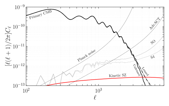
In contrast, the kSZ effect has been much more challenging to detect. Naturally, if a cluster has a large enough peculiar LOS velocity, the kSZ effect can be significant and detectable by targeted observations. This was achieved for the first time by Sayers et al. (2013) with Bolocam data collected at the Caltech Submillimeter Observatory, more recently by Adam et al. (2017) on the same system with NIKA observations at the IRAM telescope, and lastly by Sayers et al. (2019) for several galaxy clusters observed with Bolocam and AzTEC/ASTE. Nonetheless, in order to understand global properties of galaxy evolution or large-scale structure (LSS) formation, it is necessary to measure the kSZ effect averaged over a large number of objects, or over a large fraction of the sky. This can be done using large-area maps produced by CMB telescopes. The main challenges are that the resolution of CMB maps has only recently allowed us to probe the small angular scales where the kSZ effect is significant compared to the primary anisotropy of the CMB (see Figure 1), and that since the kSZ effect preserves the blackbody distribution of CMB photons, it is impossible to separate clearly from the primary CMB anisotropy in multi-frequency power spectrum analyses. Planck did not report a constraint on the amplitude of the kSZ power spectrum (Planck Collaboration, 2020b). With ACT, Choi et al. (2020) reported an upper bound, and SPT obtained a tentative $3\,\sigma$ detection (Reichardt et al., 2021). Subsequently, Gorce et al. (2022) reanalyzed the SPT data, incorporating information from Planck for constraining the parameters controlling reionization, as well as cosmology-dependent kSZ and tSZ spectra.

Figure 1: The dimensionless CMB temperature angular anisotropy power spectrum, unlensed (solid line) and lensed (dash-dotted), with the four noise curves used in our forecast analysis (Section 4) as labeled and the expected kSZ power spectrum computed in the halo model with Eq. (24) (note that this approximation slightly underestimates the total kSZ power spectrum, particularly on large scales). The CMB and kSZ power spectra assume our fiducial model (Subsection 2.1) and the noise curves are computed according to specifications given in Table 1.

Several alternative techniques have been proposed in order to overcome these challenges and obtain robust measurements of the kSZ effect. They fall into four main categories:

• The mean pairwise momentum method (Ferreira et al., 1999) uses the fact that the averaged momentum of cluster pairs should be negative when clusters are separated by a distance smaller than $\approx 25-50\,\mathrm{Mpc}$, as they tend to move towards each other due to gravity (see Calafut et al., 2021, and references therein). This method requires high-resolution CMB maps and galaxy surveys with accurate redshifts in order to reconstruct the distances between clusters and groups. Hand et al. (2012) made the first detection of the kSZ effect, applying the pairwise momentum method to data from ACT and the Sloan Digital Sky Survey III (SDSS-III) DR9 Baryon Oscillation Spectroscopic Survey (BOSS) (Eisenstein et al., 2011), followed by Planck Collaboration (2016d) using Planck maps and SDSS DR7, Soergel et al. (2016) with DES-Y1 and SPT at $4.2\,\sigma$ (using photometric rather than spectroscopic redshifts), Bernardis et al. (2017) with ACT and SDSS DR11 at $4.1\,\sigma$, and Calafut et al. (2021) reaching $5.4\,\sigma$ with ACT DR5 maps and SDSS DR15 catalogs. This method can also be implemented in Fourier space — see Sugiyama et al. (2016) for the formalism and Sugiyama et al. (2018) for a first measurement.

• The velocity-weighted stacking method relies on reconstructing the velocity field from spectroscopic galaxy surveys before stacking cut-outs of CMB maps centered at the locations of galaxies, each weighted by their LOS velocity. The velocity weights allow us to extract the correlations between the kSZ effect and the galaxies, while avoiding the velocity cancellation which would occur in a naïve approach without the weights, since the LOS velocity is as likely to be positive or negative. See Ho et al. (2009); Shao et al. (2011) for early developments of the idea and Li et al. (2014) for a presentation of the method in its more modern formulation. Planck Collaboration (2016d) and Schaan et al. (2016) applied the method using Planck maps with SDSS DR7, and ACT maps with CMASS galaxies, respectively, detecting the kSZ effect at $3$-$4\,\sigma$ significance. Recently, Schaan et al. (2021) reported a $6.5\sigma$ detection with ACT DR5 and Planck in combination with CMASS galaxies ($z\approx 0.55$, $M_{\mathrm{vir}}\approx 3\times 10^{13}M_{\odot}/h$), and Tanimura et al. (2020) obtained a $3.5\,\sigma$ detection for Planck maps and the more massive WHL clusters of the SDSS survey ($z\approx 0.25-0.55$, $M_{\mathrm{500c}}\approx 10^{14}M_{\odot}/h$).

• The projected-field method measures the cross-correlation between the square of the kSZ temperature anisotropy and a LSS tracer field, projected onto the 2D sphere. Here, the velocity cancellation is avoided via the squaring operation. In contrast to the methods described above, one challenge for the projected-field estimator is that the CMB maps must be thoroughly cleaned of foregrounds, as there is no external information about the LOS velocity field used to extract the kSZ signal from amongst the other signals in the small-scale mm-wave sky. Although this method was introduced nearly two decades ago (Doré et al., 2004; DeDeo et al., 2005), there are only two reported detections of the kSZ effect making use of it: Hill et al. (2016) cross-correlated CMB maps constructed from Planck and WMAP data with galaxies from the Wide-field Infrared Survey Explorer (WISE), and Kusiak et al. (2021) used similar CMB maps and the unWISE galaxy catalog (Krolewski et al., 2020), achieving a $5\,\sigma$ detection.

• The velocity reconstruction method measures the large-scale velocity modes via a quadratic estimator applied on a CMB map combined with a galaxy catalog (e.g., Deutsch et al., 2018; Münchmeyer et al., 2019; Sato-Polito et al., 2021; Giri & Smith, 2020; Cayuso et al., 2021; Contreras et al., 2022). (This is different from reconstructed velocities in the velocity-weighted stacking method. Here, velocities are reconstructed from the kSZ effect, rather than just the galaxy catalog.) There are no measurements with this method yet; however it is expected to become a competitive cosmological probe. For instance, Münchmeyer et al. (2019) forecast primordial non-Gaussianity constraints with CMB-S4 and VRO that are three times more sensitive than with VRO alone.

Smith et al. (2018) proved that apart from the projected-field estimator, the other three methods are mathematically equivalent, involving different ways of estimating the bispectrum $\langle T\delta_{g}\delta_{g}\rangle$, where $T$ is the CMB temperature field and $\delta_{g}$ is the galaxy overdensity field. In contrast, the projected-field estimator is a bispectrum of the form $\langle TT\delta_{g}\rangle$. Measuring the former bispectrum generally requires precise redshifts for the LSS tracers, while the latter requires precise removal of foregrounds from the CMB map.

Each method has its specific areas of applications. For instance, the pairwise momentum method is expected to become a unique probe of dark energy and modified gravity models (e.g., Kosowsky & Bhattacharya, 2009; Bull et al., 2012; Keisler & Schmidt, 2013; Mueller et al., 2015). Furthermore, with assumptions about the velocity field and in combination with tSZ measurements, it allows us to constrain the relationship between clusters’ optical depth (Battaglia, 2016; Flender et al., 2017) and Compton-$y$ parameters, probing the ICM/CGM thermodynamics, as was done for the first time using kSZ measurements in Vavagiakis et al. (2021). With the velocity-weighted stacking method, one can use aperture photometry in order to measure the shape of the gas density profile (Schaan et al., 2021) and its thermodynamics. Remarkably, Amodeo et al. (2021) constrained the parameters of the Ostriker-Bode-Babul (OBB) model (Ostriker et al., 2005) using the tSZ and kSZ measurements from Schaan et al. (2021), and found that cosmological simulations, such as Illustris TNG (Springel et al., 2017; Nelson et al., 2018) and simulations by Battaglia et al. (2010a), underpredict the CGM density and pressure at large radii.

In this paper we focus on the projected-field method for measuring the kSZ effect. We extend the theoretical formalism developed in Doré et al. (2004); DeDeo et al. (2005); Hill et al. (2016); Ferraro et al. (2016); Kusiak et al. (2021) so that we can use the projected-field power spectrum as a probe of the ionized gas density profile in and around massive halos. We do so by developing a halo-model-based approach (see, e.g., Seljak, 2000; Cooray & Sheth, 2002, for reviews of the halo model).

For general reviews of the tSZ and kSZ effects and their applications to astrophysics and cosmology, we refer to Birkinshaw (1999); Carlstrom et al. (2002); Mroczkowski et al. (2019). Nonetheless, these do not cover recent developments of applications of the tSZ and kSZ effects to cosmology, such as: growth reconstruction (e.g., Alonso et al., 2016); velocity reconstruction (see above); reionization probes (e.g., Smith & Ferraro, 2017; Ferraro & Smith, 2018; Ma et al., 2018; La Plante et al., 2020; La Plante et al., 2022; Chen et al., 2022); or the cosmological applications of the projected-field estimator that we discuss here.

The remainder of this paper is organized as follows. In the next subsections, we present our fiducial model, e.g., fiducial cosmological and astrophysical parameter values, assumptions, and the notation used throughout the paper (Subsection 2.1). In Subsection 2.2, we review key aspects of kSZ temperature fluctuations. In Subsection 2.3, we review the general formalism for the projected-field estimator. In Subsection 2.4, we review the effective approach for modeling this signal (as in Doré et al., 2004; DeDeo et al., 2005; Ferraro et al., 2016) and its numerical implementation class_sz. Section 3 is dedicated to the halo model formulation and implementation. The halo model code class_sz is described in Subsection 3.1. Subsection 3.2-3.4 contain the main material needed for the halo model calculations. The covariance matrix and lensing contribution are discussed in Subsection 3.5 and 3.6, respectively. We present forecasts for several experimental configurations and cross-correlations in Section 4. Our main results and conclusions are summarized in Section 5. Finally, we report a number of useful halo model tools and comparisons in the Appendix. In Appendix A we discuss different assumptions for the velocity dispersion. In Appendix B we present various halo model quantities and their class_sz implementation. In Appendix C we discuss in more detail some of the differences between previous studies and the new results presented here: choice of Wiener filter in Appendix C.1 and comparison with forecasts from Ferraro et al. (2016) in Appendix C.2.

2 Background

2.1 Fiducial Model, Assumptions, and Notations

We assume the homogeneous $\Lambda$ Cold Dark Matter (CDM) cosmology, on a spatially flat Friedmann-Lemaître-Robertson-Walker geometry with scale factor $a$. Our fiducial model corresponds to the Planck 2018 cosmology (last column of Table 1 in Planck Collaboration et al., 2018) with parameters: $\Omega_{c}h^{2}=0.11933$ and $\Omega_{b}h^{2}=0.02242$, the CDM and baryon density, respectively, where $h$ is the reduced Hubble parameter; $\ln(10^{10}A_{s})=3.047$ and $n_{s}=0.9665$, the amplitude and spectral index of the primordial scalar perturbation power spectrum, defined at pivot scale $k_{\mathrm{pivot}}=0.05\,\mathrm{Mpc}^{-1}$; and $\tau_{\mathrm{reio}}=0.0561$, the reionization optical depth. In our fiducial model, we consider one massive and two massless neutrino states, with total mass $\sum m_{\nu}=0.06\,\mathrm{eV}$ and an effective number of extra relativistic degrees of freedom $N_{\mathrm{eff}}=3.046$ (in order to obtain these $N_{\mathrm{eff}}$ and $\sum m_{\nu}$ values, we set the parameters $N_{\mathrm{ur}}=2.0328$ and $N_{\mathrm{ncdm}}=1$ in class_sz). As derived parameters, we have $\sigma_{8}=0.81$ for the standard deviation of the linear-theory matter density field smoothed over a sphere of $8\,\mathrm{Mpc}/h$ at $z=0$, a matter fraction $\Omega_{\mathrm{m}}=0.311$, and a baryon fraction $\Omega_{\mathrm{e}}=0.0490$, corresponding to a cosmological baryon fraction $f_{\mathrm{b}}\equiv\Omega_{\mathrm{b}}/\Omega_{\mathrm{m}}=0.156$. Furthermore, our fiducial model assumes a fully ionized ICM, with the free electron fraction $f_{\mathrm{free}}=1$ (in reality, $f_{\mathrm{free}}$ is slightly smaller than unity since some of the baryons are in the form of stars and neutral gas), and the primordial Helium abundance $Y_{\mathrm{He}}=0.245$.

For the halo abundance, we use the Tinker et al. (2008) halo mass function computed for overdensity masses $m_{\mathrm{200c}}$, i.e., the mass within the sphere enclosing 200 times the critical density at the halo redshift (see Appendix B.1 for details on the halo mass function). When needed, we convert between mass definitions and compute halo concentrations using the Bhattacharya et al. (2013) concentration-mass relation (see Appendix B.7 for details on the mass conversion). This is also our choice for calculating the halo concentration entering the NFW profile.

The goal of this paper is to apply the halo model formalism to the projected-field kSZ power spectrum. This involves computing cross-correlations between the kSZ effect and LSS tracers. In this work, we shall focus on cross-correlations with three different LSS tracers: the galaxy overdensity, $\delta_{\mathrm{g}}$; galaxy weak lensing convergence, $\kappa_{\mathrm{g}}$; and CMB weak lensing convergence, $\kappa_{\mathrm{cmb}}$.

Each tracer depends on a specific physical property of halos. The galaxy overdensity is based on a galaxy Halo Occupation Distribution (HOD), galaxy weak lensing and CMB weak lensing are based on the halo mass profiles, which we parameterize with the Navarro-Frenk-White density profile (Navarro et al., 1997), while the kSZ effect is based on the electron density profile (see Appendix B.9.2). In general, a physical property of a tracer $X$ can be written as a mass-independent redshift-dependent kernel, which we denote $W^{X}$, and a radial profile denoted $u^{X}$ that depends on the halo mass. For the Fourier transform of the profile, we use the notation $\hat{u}^{X}_{k}$.

The building blocks of halo model power spectra and bispectra are ensemble averages of Fourier transforms of the tracers’ physical properties. To simplify our expressions, we write the ensemble average over halo masses (at fixed redshift) of the Fourier transforms of the tracers’ radial profiles with the equivalent notations

$$\langle X\rangle_{n}=\langle\hat{u}^{X}_{k}\rangle_{n}=\int\hat{u}^{X}_{k}\mathrm{d}n=\int_{m_{\mathrm{min}}}^{m_{\mathrm{max}}}\hat{u}^{X}_{k}\frac{\mathrm{d}n}{\mathrm{d}m}\mathrm{d}m=\int_{\ln m_{\mathrm{min}}}^{\ln m_{\mathrm{max}}}\hat{u}^{X}_{k}\frac{\mathrm{d}n}{\mathrm{d}\ln m}\mathrm{d}\ln m,$$ (1)

where $\mathrm{d}n/\mathrm{d}m$ represents the comoving differential number density of halos per unit mass. In class_sz, we evaluate mass integrals on a logarithmic grid, as indicated in the right hand side (RHS) of the equation. Throughout the paper, we set the mass integral bounds to $m_{\mathrm{min}}=10^{10}M_{\odot}/h$ and $m_{\mathrm{max}}=3.5\times 10^{15}M_{\odot}/h$.

We write the differential number density of halos as $\mathrm{d}n/\mathrm{d}m=\mathrm{d}^{2}N/(\mathrm{d}m\,\mathrm{dv})$ where $N$ is the number of halos of mass $m$ in comoving volume per steradian $\mathrm{d}\mathrm{v}$. The comoving volume per steradian is related to the comoving distance $\chi$ via $\mathrm{dv}=\chi^{2}\mathrm{d}\chi$, with $\mathrm{d}\chi=(c/H(z))\mathrm{d}z$ where $c$ is the speed of light, $H(z)$ is the Hubble parameter, and $z$ denotes redshift.

The integrals over comoving volume, i.e., the redshift integrals, are also carried out on a logarithmic grid. In the paper, we shall use the following equivalent notations:

$$\int[\cdot\cdot\cdot]\mathrm{dv}=\int[\cdot\cdot\cdot]\chi^{2}\mathrm{d}\chi=\int_{\ln(1+z_{\mathrm{min}})}^{\ln(1+z_{\mathrm{max}})}[\cdot\cdot\cdot]\frac{c\chi^{2}}{H}(1+z)\mathrm{d}\ln(1+z).$$ (2)

For the redshift bounds we set $z_{\mathrm{min}}=0.005$ and $z_{\mathrm{max}}=3$. The lower bound is chosen to avoid spurious numerical divergence at $z=0$. We checked that as long as the value is small enough, our predictions are unchanged by different $z_{\mathrm{min}}$. The upper bound is chosen so that we do not need to extrapolate the redshift dependence of quantities calibrated on simulations (e.g., the halo mass function, gas density profiles, etc.). For kSZ² - CMB lensing cross-correlation, although the lensing kernel peaks at $z\sim 2$, we note that we are missing some contribution from $z>3$. We leave a detailed study of the high redshift contribution to future works, as it implies using a suited optical depth evolution and halo mass function which are outside the scope of this paper.

To go from 3D spectra (power spectra or bispectra) to 2D angular spectra, i.e., by projecting along the LOS, we work within the Limber approximation on the flat sky (Limber, 1957), such that 3D wavenumber $k$ is mapped to 2D angular multipole $\ell$ via

$$k=(\ell+1/2)/\chi.$$ (3)

Thus, in the paper, we often use $k$ and $\ell$ interchangeably. We refer the reader to Appendix A of Hill & Pajer (2013) for a detailed discussion on the Limber/flat-sky approximation in this context.

2.2 Kinetic SZ Anisotropy

The CMB temperature fluctuation due to the kSZ effect, $\Theta^{\mathrm{kSZ}}=\Delta T/\bar{T}$ where $\bar{T}$ is the mean CMB temperature, is sourced by the visibility-weighted electron velocity field projected along the LOS. In a direction ${\mathbf{n}}$, it can be written as

$$\Theta^{\mathrm{kSZ}}({\mathbf{n}})=-\frac{1}{c}\int\mathrm{d}\chi\,g(\bm{x}){\mathbf{n}}\cdot\bm{v_{e}}(\bm{x}),$$ (4)

where $\bm{v_{e}}$ is the electron velocity at $\bm{x}=(\chi,{\mathbf{n}}$) and $g$ is the visibility function, i.e., the probability of scattering within $\mathrm{d}\chi$, given by

$$g=\frac{\mathrm{d}\tau}{\mathrm{d}\chi}e^{-\tau}\quad\mathrm{with}\quad\frac{\mathrm{d}\tau}{\mathrm{d}\chi}=\frac{\dot{\tau}}{c}=a\sigma_{\mathrm{T}}n_{\mathrm{e}}$$ (5)

where the overdot represents a derivative with respect to conformal time $\eta=\int\mathrm{d}t/a$, and where $\sigma_{\mathrm{T}}=6.985\times 10^{-74}\,\mathrm{Mpc}^{2}$ is the Thomson scattering cross-section. We express the electron number density along the LOS as

$$n_{\mathrm{e}}=\frac{\rho_{\mathrm{gas,free}}}{m_{\mathrm{u}}\mu_{\mathrm{e}}}\quad\mathrm{with}\quad\rho_{\mathrm{gas,free}}=f_{\mathrm{free}}\rho_{\mathrm{gas}}:=\rho_{\mathrm{e}}$$ (6)

where $m_{\mathrm{u}}$ is the atomic mass unit and $\mu_{\mathrm{e}}=(1-Y_{\mathrm{He}}/2)^{-1}\simeq 1.14$ is the mean molecular weight per electron. We emphasize that in this expression, the free electron fraction $f_{\mathrm{free}}$ represents the fraction of the gas that is fully ionized — for instance, this excludes stars. For galaxy clusters, we assume $\tau\ll 1$ (e.g., Battaglia, 2016; Flender et al., 2017) and $e^{-\tau}\approx 1$ throughout the paper. In Eq. (6) the homogeneous part of electron density is given by (assuming $\bar{\rho}_{\mathrm{gas}}=\bar{\rho}_{\mathrm{b}}$)

$$\bar{\rho}_{\mathrm{e}}=f_{\rm free}\bar{\rho}_{\mathrm{b}}=f_{\rm free}\Omega_{\mathrm{b}}\rho_{\mathrm{crit,0}}(1+z)^{3}=f_{\rm free}f_{\rm b}\rho_{\mathrm{m,0}}(1+z)^{3}$$ (7)

where $f_{\mathrm{b}}=\Omega_{\mathrm{b}}/\Omega_{\mathrm{m}}$ is the baryon fraction.

Since the visibility function is proportional to the baryon density, inhomogeneities of the baryon density field are associated with inhomogeneities of the visibility function. At leading order, we have

$$g=\bar{g}+\delta g\quad\mathrm{with}\quad\delta g=\frac{\bar{g}}{f_{\mathrm{b}}f_{\mathrm{free}}}\delta_{\mathrm{e}}\quad\mathrm{and}\quad\delta_{\mathrm{e}}=\frac{\delta\rho_{\mathrm{e}}}{\rho_{\mathrm{m}}},$$ (8)

where $\bar{g}$ is the homogeneous part of the visibility function computed with Eq. (5) using $\bar{\rho}_{\mathrm{e}}$ in Eq. (6), and $\delta g$ is the fluctuation caused by inhomogeneities of the electron density. Note the here, we do not consider fluctuations caused by patchy reionization, as we focus on the LSS formation era at lower redshift.

In Eq. (8) we wrote our definition of the electron density perturbation with respect to the mean matter density. With this convention, the power spectrum $P_{\delta_{\mathrm{e}}\delta_{\mathrm{e}}}$ vanishes for $\rho_{\mathrm{e}}\rightarrow 0$. Moreover, with $\rho_{\mathrm{e}}=f_{\mathrm{b}}f_{\mathrm{free}}\rho_{\mathrm{m}}$, we have $P_{\delta_{\mathrm{e}}\delta_{\mathrm{e}}}\sim(f_{\mathrm{b}}f_{\mathrm{free}})^{2}P_{L}$ (on large scales).

Plugging Eq. (8) into Eq. (4), we can rewrite the temperature fluctuation as

$$\Theta^{\mathrm{kSZ}}({\mathbf{n}})=-\frac{1}{c}\int\mathrm{d}\chi\,\bar{g}(\chi){\mathbf{n}}\cdot\bm{\tilde{v}_{\mathrm{e}}}(\bm{x})\quad\mathrm{with}\quad\bm{\tilde{v}_{\mathrm{e}}}(\bm{x})=\bm{{v}_{\mathrm{e}}}(\bm{x})+\frac{1}{f_{\mathrm{b}}f_{\mathrm{free}}}\delta_{\mathrm{e}}(\bm{x})\bm{v_{\mathrm{e}}}(\bm{x}).$$ (9)

In Fourier space, the velocity field $\bm{\tilde{v}_{\mathrm{e}}}$ is

$$\hat{\bm{\tilde{v}}}_{\bm{e}}(\bm{k})=\hat{\bm{v}}_{\bm{\mathrm{e}}}(\bm{k})+\frac{1}{f_{\mathrm{b}}f_{\mathrm{free}}}\int\frac{\mathrm{d}^{3}\bm{k}^{\prime}}{(2\pi)^{3}}\hat{\delta}_{\mathrm{e}}(|\bm{k}-\bm{k}^{\prime}|)\hat{\bm{v}}_{\bm{\mathrm{e}}}(\bm{k}^{\prime}).$$ (10)

The second term on the RHS is the velocity field modulated by the density perturbation. Note that since $\bm{v_{\mathrm{e}}}$ is a first-order quantity, this term is second order in perturbations. Let us introduce the longitudinal and transverse components of the velocity field in Fourier space, with respect to the mode $\bm{k}=k\bf{k}$:

$$\hat{\bm{\tilde{v}}}_{\bm{e}}=\hat{\bm{\tilde{v}}}_{\bm{e}}^{||}+\hat{\bm{\tilde{v}}}_{\bm{e}}^{\perp}\quad\mathrm{with}\quad\hat{\bm{\tilde{v}}}_{\bm{e}}^{||}=(\hat{\bm{\tilde{v}}}_{\bm{e}}\cdot{\bf{k}}){\bf{k}}\quad\mathrm{and}\quad\hat{\bm{\tilde{v}}}_{\bm{e}}^{\perp}=\hat{\bm{\tilde{v}}}_{\bm{e}}-(\hat{\bm{\tilde{v}}}_{\bm{e}}\cdot\bf{k})\bf{k}$$ (11)

We note that in standard cosmological perturbation theory, the vortical components of the matter velocity field can be neglected, hence we can assume that $\bm{{v}_{\mathrm{e}}}$ is longitudinal, i.e., $\hat{\bm{{v}}}_{\bm{\mathrm{e}}}(\bm{k})=\hat{v}_{{\mathrm{e}}}(k)\bf{k}$ (this is valid to all orders in perturbation, see, e.g., Dodelson & Schmidt, 2020). Then the longitudinal component is

$$\hat{\tilde{v}}_{e}^{||}(k)=\hat{v}_{{\mathrm{e}}}(k)+\frac{1}{f_{\mathrm{b}}f_{\mathrm{free}}}\int\frac{\mathrm{d}^{3}\bm{k}^{\prime}}{(2\pi)^{3}}\hat{\delta}_{\mathrm{e}}(|\bm{k}-\bm{k}^{\prime}|)\hat{v}_{{\mathrm{e}}}(k^{\prime})\mu,\quad\mathrm{with}\quad\mu=\bf{k}^{\prime}\cdot\bf{k}.$$ (12)

For the transverse component, we get

$$\hat{\bm{\tilde{v}}}_{\bm{e}}^{\perp}=\frac{1}{f_{\mathrm{b}}f_{\mathrm{free}}}\int\frac{\mathrm{d}^{3}\bm{k}^{\prime}}{(2\pi)^{3}}\hat{\delta}_{\mathrm{e}}(|\bm{k}-\bm{k}^{\prime}|)\hat{v}_{{\mathrm{e}}}(k^{\prime})({\bf{k}}^{\prime}-\mu{\bf{k}}).$$ (13)

Thus, at leading order, the total velocity field is purely longitudinal, with amplitude (in linear theory):

$$\hat{v}_{\mathrm{e}}(k)=-iaHf\hat{\delta}_{\mathrm{m}}(k)/k\,\quad\mathrm{with}\quad f=\frac{\mathrm{d}\ln D}{\mathrm{d}\ln a}$$ (14)

the growth rate and where $D$ is the growth factor (e.g., Dodelson & Schmidt, 2020).

Next, there is a second-order contribution of the form $\delta v$ (the last term in Eq. (12)). The transverse component $\hat{\bm{\tilde{v}}}_{\bm{e}}^{\perp}$ is purely of the form $\delta v$, i.e., a second-order quantity. The longitudinal component $\hat{\bm{\tilde{v}}}_{\bm{e}}^{||}$ cannot contribute to the kSZ anisotropy at small scales, because of the cancellation of crests and troughs when projected along the line of sight (e.g., Jaffe & Kamionkowski, 1998). Therefore, at leading order in perturbations, the kSZ effect vanishes for small inhomogenieties (Kaiser, 1984). Hence, the kSZ anisotropy, on small scales, is generated by the transverse, second-order term, $\hat{\bm{\tilde{v}}}_{\bm{e}}^{\perp}$. (Schematically, ${\bf{n}}\cdot\hat{\bm{\tilde{v}}}_{\bm{e}}\approx{\bf{n}}\cdot\hat{\bm{\tilde{v}}}_{\bm{e}}^{\perp}$ for small inhomogeneities.) Then, when $\delta_{\mathrm{e}}$ is in the linear regime, the kSZ anisotropy is called the Ostriker-Vishniac (OV) effect (Ostriker & Vishniac, 1986; Vishniac, 1987). The large-scale kSZ anisotropy from the linear Doppler effect and the OV effect are important during reionization. They are not of direct interest here, since we focus on the anisotropy generated in collapsed regions of the density field (halos) where $\delta_{\mathrm{e}}$ is non-linear, i.e., the kSZ effect from large-scale structure. Nonetheless, to understand how different terms and scales play out, even in the non-linear regime, it is instructive to review the main aspects of the OV power spectrum calculation — see Hu (2000); Ma & Fry (2002), and Park et al. (2013) or Appendix B of Alvarez (2016) for a thorough derivation.

The key quantity to evaluate is the 3D power spectrum of the transverse component (i.e., the curl) of the density-modulated velocity field, $P_{\perp}$, defined via

$$\langle\hat{\bm{\tilde{v}}}_{\bm{e}}^{\perp}(\bm{k})\hat{\bm{\tilde{v}}}_{\bm{e}}^{\perp}(\bm{k}^{\prime})^{*}\rangle=(2\pi)^{3}P_{\perp}(k,\chi)\delta_{D}(\bm{k}^{\prime}-\bm{k})$$ (15)

where $\delta_{D}$ is the Dirac delta function. Once this is known, the angular anisotropy power spectrum of the kSZ effect can be written as

$$C_{\ell}^{\mathrm{kSZ}}=\frac{1}{2c^{2}}\int\mathrm{d}\chi\frac{\bar{g}^{2}}{\chi^{2}}P_{\perp}(k,\chi)\quad\mathrm{with}\quad k=(\ell+1/2)/\chi,$$ (16)

where the pre-factor 1/2 comes from the projection along the LOS (see, e.g., Jaffe & Kamionkowski, 1998; Park et al., 2013, for the derivation of the pre-factor). Schematically, $P_{\perp}$ has three terms since

$$\langle\delta v\delta v\rangle\sim\langle\delta\delta\rangle\langle vv\rangle+\langle\delta v\rangle\langle\delta v\rangle+\langle\delta v\delta v\rangle_{c}.$$ (17)

The last term is the connected term, expected to be subdominant (see Ma & Fry, 2002; McQuinn et al., 2005; Park et al., 2016), and is neglected hereafter. The first and second terms can be evaluated straightforwardly, yielding

$$P_{\perp}(k,\chi)=\frac{1}{(2\pi f_{\mathrm{b}}f_{\mathrm{free}})^{2}}\int\mathrm{d}k^{\prime}k^{\prime 2}\int\mathrm{d}\mu(1-\mu^{2})\left[P_{\delta_{\mathrm{e}}\delta_{\mathrm{e}}}(|\bm{k}-\bm{k}^{\prime}|)P_{v_{\mathrm{e}}v_{\mathrm{e}}}(k^{\prime})-\frac{k^{\prime}}{|\bm{k}-\bm{k}^{\prime}|}P_{\delta_{\mathrm{e}}v_{\mathrm{e}}}(|\bm{k}-\bm{k}^{\prime}|)P_{\delta_{\mathrm{e}}v_{\mathrm{e}}}(k^{\prime})\right]$$ (18)

where we used the definitions

$$\langle\hat{\delta}_{\mathrm{e}}(\bm{k})\hat{\delta}_{\mathrm{e}}(\bm{k}^{\prime})\rangle=(2\pi)^{3}P_{\delta_{\mathrm{e}}\delta_{\mathrm{e}}}\delta_{D}(\bm{k}+\bm{k}^{\prime})\quad\mathrm{and}\quad\langle\hat{\delta}_{\mathrm{e}}(\bm{k})\hat{v}_{\mathrm{e}}(\bm{k}^{\prime})\rangle=(2\pi)^{3}P_{\delta_{\mathrm{e}}v_{\mathrm{e}}}\delta_{D}(\bm{k}+\bm{k}^{\prime}).$$ (19)

With the velocity from linear perturbation theory (Eq. (14)), we can further simplify Eq. (18), since

$$P_{v_{\mathrm{e}}v_{\mathrm{e}}}(k)=(aHf/k)^{2}P_{\delta_{\mathrm{m}}\delta_{\mathrm{m}}}(k)\quad\mathrm{and}\quad P_{\delta_{\mathrm{e}}v_{\mathrm{e}}}(k)=(aHf/k)P_{\delta_{\mathrm{e}}\delta_{\mathrm{m}}}(k)\,.$$ (20)

The final expression reads

$$P^{\mathrm{OV}}_{\perp}(k,\chi)=\frac{(aHf)^{2}}{(2\pi f_{\mathrm{b}}f_{\mathrm{free}})^{2}}\int\mathrm{d}k^{\prime}\int\mathrm{d}\mu(1-\mu^{2})P_{\delta_{\mathrm{e}}\delta_{\mathrm{e}}}(|\bm{k}-\bm{k}^{\prime}|)P_{\delta_{\mathrm{e}}\delta_{\mathrm{e}}}(k^{\prime})\frac{k(k-2k^{\prime}\mu)}{k^{2}+k^{\prime 2}-2kk^{\prime}\mu}\,,$$ (21)

which is the well-known OV approximation of Eq. (18).

Let us now turn to the non-linear regime. First, we define the volume-averaged velocity dispersion

$$\sigma_{v}^{2}(\chi)\equiv\frac{v_{\mathrm{rms}}^{2}(\chi)}{3c^{2}}\quad\mathrm{with}\quad v_{\mathrm{rms}}^{2}(\chi)=\frac{1}{2\pi^{2}}\int\mathrm{d}k\,k^{2}P_{v_{\mathrm{e}}v_{\mathrm{e}}}\left(k,\chi\right).$$ (22)

In the high-$k$ (non-linear) regime, we can drop terms of $\mathcal{O}(k^{\prime}/k)$ in Eq. (18), including $P_{\delta_{\mathrm{e}}v_{\mathrm{e}}}$ (e.g., Hu, 2000; Ma & Fry, 2002; McQuinn et al., 2005). Hence, $P_{\delta_{\mathrm{e}}\delta_{\mathrm{e}}}(|\bm{k}-\bm{k}^{\prime}|)\approx P_{\delta_{\mathrm{e}}\delta_{\mathrm{e}}}(k)$ and the integral over $\mu$ can be carried out (yielding a factor $4/3$). One finds

$$P^{\mathrm{high-}k}_{\perp}(k,\chi)=\frac{2}{3}\frac{(v_{\mathrm{rms}}/c)^{2}}{(f_{\mathrm{b}}f_{\mathrm{free}})^{2}}P_{\delta_{\mathrm{e}}\delta_{\mathrm{e}}}(k,\chi)=\frac{2\sigma_{v}^{2}}{(f_{\mathrm{b}}f_{\mathrm{free}})^{2}}P_{\delta_{\mathrm{e}}\delta_{\mathrm{e}}}(k,\chi)$$ (23)

so that in this regime, the angular anisotropy power spectrum reads

$$C_{\ell}^{\mathrm{kSZ,\,high-}k}=\int\mathrm{d}\mathrm{v}W^{\mathrm{kSZ}}(\chi)^{2}P_{\delta_{\mathrm{e}}\delta_{\mathrm{e}}}\left(k,\chi\right)\quad\mathrm{with}\quad W^{\mathrm{kSZ}}(\chi)=\frac{a\sigma_{\mathrm{T}}\bar{\rho}_{\mathrm{m}}\sigma_{v}}{m_{\mu}\mu_{e}\chi^{2}}.$$ (24)

In the equation above, the $(f_{\mathrm{b}}f_{\mathrm{free}})^{2}$ factor of Eq. (23) is canceled by the same factor that appears in $\bar{g}$. In order to evaluate the velocity dispersion $\sigma_{v}$, we can use the linear theory ansatz for $P_{v_{\mathrm{e}}v_{\mathrm{e}}}$ (see Eq. (20)) and assume $P_{\delta_{\mathrm{e}}\delta_{\mathrm{e}}}\approx(f_{b}f_{\mathrm{free}})^{2}P_{\delta_{\mathrm{m}}\delta_{\mathrm{m}}}$, where $P_{\delta_{\mathrm{m}}\delta_{\mathrm{m}}}$ is the matter power spectrum. Here, the matter power spectrum can either be the linear matter power spectrum $P_{L}$ or the non-linear matter power spectrum $P_{NL}$ from halofit (Smith et al., 2003; Takahashi et al., 2012) or hmcode (Mead et al., 2015, 2021). See Appendix A and Figure 15 for a comparison of these different choices. Meanwhile, the electron power spectrum $P_{\delta_{\mathrm{e}}\delta_{\mathrm{e}}}$ that appears explicitly in Eq. (24) is computed using the halo model (see Appendix B.9.2).

2.3 Projected-field kSZ Estimator

Consider a large-scale structure tracer $X$ that does not depend linearly on the velocity field. For instance, in this paper, we shall work with the galaxy number density $X=\delta_{\mathrm{g}}$, galaxy weak lensing convergence $X=\kappa_{\mathrm{g}}$, and CMB lensing convergence $X=\kappa_{\mathrm{cmb}}$. Since the kSZ anisotropy is proportional to the bulk velocity of the electrons, the cross-correlation $\langle X\Theta^{\mathrm{kSZ}}\rangle$ vanishes (at first order) simply due to sign cancellation because of the isotropy of the velocity field: collapsed regions are as likely to be in a “positive” or “negative” bulk motion with respect to the LOS.

To probe such correlations, we can resort to higher-order statistics (e.g., Cooray, 2001). Doré et al. (2004) proposed to work with a three-point statistic: two kSZ points, so that the statistic is even in the velocity, and one point in $X$. They introduced a collapsed three-point function, that is, the cross-correlation between the squared kSZ field and $X$. This condenses the information of the full bispectrum into an angular power spectrum that is arguably more easily measurable, the so-called projected-field kSZ power spectrum denoted $C_{\ell}^{\mathrm{kSZ^{2}}X}$.

Figure 2: (Left:) The Wiener filter of Eq. (25). (Right:) The product of the filter and beam (see Eq. 27). We use the specifications of Table 1 (see also Section 4) and our fiducial model to compute these filters. Except for Planck that has $\ell_{\mathrm{max}}=3000$, we use $\ell_{\mathrm{max}}=8000$ for all other filters. (See footnote 5 for the high-$\ell$ taper.)

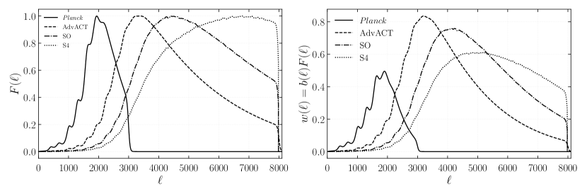
In practice, the projected-field kSZ power spectrum is measured by squaring a CMB temperature map in real space before cross-correlating it with a map of tracer $X$ in harmonic space. Furthermore, in order to maximize the contribution from arcminute scales where the kSZ effect is more significant, the temperature map is Wiener-filtered in harmonic space beforehand:

$$\Theta_{f}(\bm{\ell})\equiv\Theta(\bm{\ell})\quad\mathrm{with}\quad w(\ell)=b(\ell)F(\ell)\quad\mathrm{where}\quad F(\ell)\equiv\frac{\sqrt{C_{\ell}^{\mathrm{kSZ}}}/C_{\ell}^{\mathrm{tot}}}{\mathrm{max}(\sqrt{C_{\ell}^{\mathrm{kSZ}}}/C_{\ell}^{\mathrm{tot}})}$$ (25)

is our ansatz for the optimal filter. This filter choice differs from previous works (e.g. Hill et al., 2016; Ferraro et al., 2016; Kusiak et al., 2021) which did not use a square root — we explain this difference in Appendix C.1, justifying why it is more optimal. In Eq. (25), $\Theta_{f}$ is the temperature anisotropy of the filtered CMB map, $\Theta$ is the temperature anisotropy of the unfiltered CMB map, $C_{\ell}^{\mathrm{kSZ}}$ is the power spectrum of the kSZ effect which we compute according to Eq. (24) within our fiducial model, and $C_{\ell}^{\mathrm{tot}}$ is the angular power spectrum of the map, which in principle contains contributions from the lensed primary CMB, ISW, the kSZ anisotropy (from both reionization and galaxy clusters), as well as all residual foregrounds (e.g., tSZ and CIB), and instrumental and atmospheric noise. In this paper, we compute $C_{\ell}^{\mathrm{tot}}$ as a sum of the lensed CMB power spectrum from class/class_sz (with our fiducial parameters), the kSZ power spectrum, and the noise curves for a given CMB experiment, e.g., Planck, AdvACT, SO, or CMB-S4, namely:

$$C_{\ell}^{\mathrm{tot}}=C_{\ell}^{\Theta\Theta,\mathrm{lensed}}+C_{\ell}^{\mathrm{kSZ}}+N_{\ell}^{\Theta\Theta}.$$ (26)

In filtering operation, to mitigate divergences due to large noise at small scales, we also include a Gaussian beam window function:

$$b(\ell)=\mathrm{exp}\left\{-\tfrac{1}{2}\ell(\ell+1)\frac{\theta_{\mathrm{FWHM}}^{2}}{8\ln 2}\right\}$$ (27)

where $\theta_{\mathrm{FWHM}}$ is the full width at half maximum (FWHM) of the telescope’s beam in radians (in terms of the analysis, it is equivalent to leaving the beam in the observed CMB temperature map when computing the power spectra). The experimental configurations considered in this analysis are specified in Table 1.

Then, in harmonic space (where the real space product becomes a convolution) the projected-field power spectrum estimator dubbed $\bar{C}_{\ell}^{\mathrm{kSZ^{2}}X}$ is defined via

$$\langle\Theta_{f}^{2}(\bm{\ell}^{\prime})X(\bm{\ell})\rangle=\int\frac{\mathrm{d}^{2}\bm{\ell}^{\prime\prime}}{(2\pi)^{2}}\langle\Theta_{f}(\bm{\ell}^{\prime\prime})\Theta_{f}(\bm{\ell}^{\prime}-\bm{\ell}^{\prime\prime})X(\bm{\ell})\rangle=(2\pi)^{2}\delta_{D}(\bm{\ell}+\bm{\ell}^{\prime})\bar{C}_{\ell}^{\mathrm{kSZ^{2}}X}.$$ (28)

Let us now make the connection between the projected-field kSZ power spectrum and the kSZ anisotropy. As we saw in the previous subsection, the kSZ anisotropy is sourced by the velocity field $\bm{v_{e}}$ projected along the LOS. Moreover, we saw that only transverse modes contribute to the kSZ effect in the high-$k$ regime. Thus, it is natural to introduce the three-point function

$$\langle\hat{\bm{\tilde{v}}}_{\bm{e}}^{\perp}(\bm{k})\hat{\bm{\tilde{v}}}_{\bm{e}}^{\perp}(\bm{k}^{\prime})\hat{X}(\bm{k}^{\prime\prime})\rangle=(2\pi)^{3}\delta_{D}(\bm{k}+\bm{k}^{\prime}+\bm{k}^{\prime\prime})\mathcal{C}_{v_{e}^{2}X}(\bm{k},\bm{k}^{\prime},\bm{k}^{\prime\prime}),$$ (29)

where $\mathcal{C}_{v_{e}^{2}X}$ is the analogue of $P_{\perp}$ (see Eq. (15)). Since $\hat{\bm{\tilde{v}}}_{\bm{e}}^{\perp}\sim\delta v$, it is a contraction of the five-point function that can be schematically written as

$$\langle\delta v\delta v\delta_{X}\rangle\sim\langle\delta\delta\rangle\langle vv\delta_{X}\rangle+\langle\delta v\rangle\langle\delta v\delta_{X}\rangle+\langle vv\rangle\langle\delta\delta\delta_{X}\rangle+\dotsb+\langle\delta v\delta v\delta_{X}\rangle_{c},$$ (30)

where the last term is the connected term and where $\delta_{X}$ denotes the perturbation for the tracer $X$. Doré et al. (2004) only took into account the third term in this expansion. DeDeo et al. (2005) studied the relative importance of each of these terms (see their Figure 1), following a similar approach as Ma & Fry (2002) did for the power spectrum, and concluded that the Doré et al. (2004) approach was a good approximation. Its validity was further confirmed by comparison to numerical simulations in Hill et al. (2016) and Ferraro et al. (2016). Here, we shall work with the same approximation, namely, $\mathcal{C}_{v_{e}^{2}X}\approx\langle vv\rangle\langle\delta\delta\delta_{X}\rangle$, so that (as in Eq. (23)):

$$\mathcal{C}_{v_{e}^{2}X}\approx\frac{2\sigma_{v}^{2}}{(f_{\mathrm{b}}f_{\mathrm{free}})^{2}}B_{\delta_{\mathrm{e}}\delta_{\mathrm{e}}X}$$ (31)

where $\sigma_{v}^{2}$ is the velocity dispersion defined in Eq. (22) and $B_{\delta_{\mathrm{e}}\delta_{\mathrm{e}}X}$ is the hybrid bispectrum of baryon density perturbations and $X$ (Doré et al., 2004). Assuming temporarily $\Theta=\Theta^{\mathrm{kSZ}}$ and combining Eqs. (31), (29), and (28), we can write the projected-field kSZ power spectrum as

$$C_{\ell}^{\mathrm{kSZ}^{2}X}=\int\mathrm{dv}W^{\mathrm{kSZ}}(\chi)^{2}W^{X}(\chi)T(\ell,\chi)\quad\mathrm{with}\quad T(\ell,\chi)=\int\frac{\mathrm{d}^{2}\bm{\ell}^{\prime}}{(2\pi)^{2}}w(\ell^{\prime})w(\left|\bm{\ell}+\bm{\ell}^{\prime}\right|)B_{\delta_{\mathrm{e}}\delta_{\mathrm{e}}X}(\mathbf{k}_{1},\mathbf{k}_{2},\mathbf{k}_{3})$$ (32)

with wavenumbers $\mathbf{k}_{1}\chi=\bm{\ell}^{\prime}$, $\mathbf{k}_{2}\chi=-(\bm{\ell}+\bm{\ell}^{\prime})$, $\mathbf{k}_{3}\chi=\bm{\ell}$ such that $\mathbf{k}_{1}+\mathbf{k}_{2}+\mathbf{k}_{3}=\vec{0}$, where $W^{X}(\chi)$ is the projection kernel of the tracer $X$, and $W^{\mathrm{kSZ}}(\chi)$ is the projection kernel of the kSZ effect defined in Eq. (24). Here, $T(\ell,\chi)$ is the so-called triangle power spectrum: it is a sum over all triangle configurations with sides $(\bm{\ell},\bm{\ell}^{\prime},-\bm{\ell}-\bm{\ell}^{\prime})$ in planes perpendicular to the LOS, at constant redshift (Doré et al., 2004).

The remaining task is to find an expression for the hybrid bispectrum. With this aim, in the next Subsection we revisit the approach that was adopted in previous works (Doré et al., 2004; DeDeo et al., 2005; Hill et al., 2016; Ferraro et al., 2016; Kusiak et al., 2021), and in Section 3 we present our newly developed halo model.

	$\Theta_{\mathrm{FWHM}}$	$\Delta_{T}$
	(arcmin)	($\mu$K-arcmin)	$\ell_{\mathrm{max}}$	$f_{\mathrm{sky}}$
Planck	$5$	$47$	$3000$	0.6
AdvACT	$1.5$	$20$	$8000$	0.3
SO and CMB-S4	$1.4$	ILC	$8000$	0.4

Table 1: Specifications of the CMB experiments (Planck, AdvACT, SO, and CMB-S4) used in the forecast analysis. $\Theta_{\mathrm{FWHM}}$ denotes the full width at half maximum (FWHM) of the telescope beam, $\ell_{\mathrm{max}}$ is the multipole that determines the transition to zero of the Wiener filter (see Eq. 25), and $f_{\mathrm{sky}}$ denotes the sky fraction after relevant masks have been applied to the surveyed CMB sky area. See Section 4 for further details.

2.4 Effective Approach

The task of finding an expression for the hybrid bispectrum $B_{\delta_{\mathrm{e}}\delta_{\mathrm{e}}X}$ can be simplified significantly under some assumptions. First, if the baryons are assumed to perfectly trace the dark matter density field, we can write $\delta_{\mathrm{e}}=f_{\mathrm{b}}f_{\mathrm{free}}\delta_{\mathrm{m}}$. Second, if the tracer $X$ is also a tracer of the density field, we have $\delta_{X}=b_{X}\delta_{\mathrm{m}}$, where $b_{X}$ is the bias of $X$. For instance, for the galaxy density field $b_{X}$ is the galaxy bias, while for CMB or galaxy weak lensing $b_{X}=1$. With these two assumptions, the hybrid bispectrum reduces to $B_{\delta_{\mathrm{e}}\delta_{\mathrm{e}}X}=b_{X}(f_{\mathrm{b}}f_{\mathrm{free}})^{2}B_{\mathrm{m}}$, where $B_{\mathrm{m}}$ is the matter bispectrum.

In analogy with the calculation of the kSZ power spectrum in the high-$k$ regime, where the baryon density power spectrum can by approximated with the non-linear matter power spectrum calibrated on $N$-body simulations, Doré et al. (2004) and DeDeo et al. (2005) used a non-linear matter bispectrum fitting formula from Scoccimarro & Couchman (2001). Similarly, Hill et al. (2016); Ferraro et al. (2016); Kusiak et al. (2021) used the fit from Gil-Marín et al. (2012), which improves upon Scoccimarro & Couchman (2001) while keeping the same functional form. These bispectrum fitting functions are based on the expression of the tree-level matter bispectrum in Eulerian perturbation theory, for an Einstein de-Sitter Universe (Fry, 1984)

$$B_{\mathrm{TL}}(k_{1},k_{2},k_{3})=2F_{2}(k_{1},k_{2},k_{3})P_{L}(k_{1})P_{L}(k_{2})+2\,\mathrm{cyc.}$$ (33)

where we did not write explicitly the permutations between modes and where the $F_{2}$ kernel is given by (Fry, 1984; Goroff et al., 1986)

$$F_{2}(k_{1},k_{2},k_{3})=F_{2}(\mathbf{k}_{1},\mathbf{k}_{2})=\frac{5}{7}+\frac{1}{2}\cos\theta_{12}\left(\frac{k_{1}}{k_{2}}+\frac{k_{2}}{k_{1}}\right)+\frac{2}{7}(\cos\theta_{12})^{2}\quad\mathrm{with}\quad\cos\theta_{12}=\frac{\mathbf{k}_{1}\cdot\mathbf{k}_{2}}{k_{1}k_{2}}=\frac{k_{3}^{2}-k_{2}^{2}-k_{1}^{2}}{2k_{1}k_{2}}.$$ (34)

(This is the expression as implemented in class_sz, which takes the three wavenumber moduli as an input.) The Gil-Marín et al. (2012) bispectrum fitting formula has the same form as Eq. (33), except that the linear matter power spectrum is replaced by its non-linear counterpart and that it includes extra scale- and redshift-dependent coefficients in front of the terms in the expression of the $F_{2}$ kernel. There are nine parameters that control the scale and redshift dependence of those coefficients, whose values are found by fitting the data from $N$-body simulations. Thus, the non-linear matter bispectrum is written as

$$B_{\mathrm{eff}}^{NL}(k_{1},k_{2},k_{3})=2F_{2}^{\mathrm{eff}}(k_{1},k_{2},k_{3})P_{NL}(k_{1})P_{NL}(k_{2})+2\,\mathrm{cyc}.$$ (35)

See Eqs. 2.6-2.12 of Gil-Marín et al. (2012) for the expression of the effective kernel $F_{2}^{\mathrm{eff}}$, as well as the values of the fitting parameters.

The non-linear matter bispectrum computed with the Gil-Marín et al. (2012) and Scoccimarro & Couchman (2001) fitting formulas are plotted in the top panels of Figure 3. The main difference between these formulas is that the Gil-Marín et al. (2012) formula corrects the unphysical oscillations associated with the BAOs in the power spectrum which are visible in the Scoccimarro & Couchman (2001) prediction (see, e.g., Gil-Marín et al., 2012, for details). On large scales, both formulas match with the tree-level bispectrum of Eq. (33). Note that the Gil-Marín et al. (2012) formula is calibrated on a fairly restricted $k$- and $z$-range compared to what may be needed for kSZ applications, namely: $0.03\,h/\mathrm{Mpc}\leq k\leq 0.4h/\mathrm{Mpc}$, and $0\leq z\leq 1.5$. Recent matter bispectrum fitting formulas have been derived by Takahashi et al. (2020) on a broader $k$- and $z$-range ($k\lesssim 3h/\mathrm{Mpc}$ and $z<3$) but we do not discuss them here as they have not been used in the context of the kSZ effect.

In what we shall refer to as the effective approach projected-field kSZ power spectrum hereafter, the hybrid bispectrum in Eq. (32) is approximated by $b_{X}f_{\mathrm{b}}^{2}f_{\mathrm{free}}^{2}B_{\mathrm{eff}}^{NL}$ of Eq. (35). While the numerical evaluation of Eq. (35) is fast and straightforward, the computation of $C_{\ell}^{\mathrm{kSZ}^{2}X}$ is more involved and takes several minutes on a laptop. In class_sz, the computation is parallelized with respect to multipoles $\ell$. Then, at each $\ell$ we tabulate the redshift integrals

$$I_{\ell}(\ell^{\prime},\theta)=\int\mathrm{dv}\,W^{\mathrm{kSZ}}(\chi)^{2}W^{X}(\chi)b_{X}f_{\mathrm{b}}^{2}f_{\mathrm{free}}^{2}B_{\mathrm{eff}}^{NL}(\ell^{\prime}/\chi,\left|\bm{\ell}+\bm{\ell}^{\prime}\right|/\chi,\ell/\chi)$$ (36)

on a 2D grid spanned by $\ln\ell^{\prime}$ and the polar angle $\theta=(\hat{\bm{\ell},\bm{\ell}^{\prime}})$. Note that the dependence on $\theta$ arises from the modulus $\left|\bm{\ell}+\bm{\ell}^{\prime}\right|$ that appears in the bispectrum (since $\left|\bm{\ell}+\bm{\ell}^{\prime}\right|^{2}=\ell^{2}+\ell^{\prime 2}+2\ell\ell^{\prime}\cos\theta$). Then we integrate over $\ln\ell^{\prime}$ at fixed $\theta$, and eventually over $\theta$, i.e.,

$$C_{\ell}^{\mathrm{kSZ}^{2}X}=\frac{1}{2\pi^{2}}\int_{0}^{\pi}\mathrm{d}\theta\int\mathrm{d}\ln\ell^{\prime}\ell^{\prime 2}w(\ell^{\prime})w(\left|\bm{\ell}+\bm{\ell}^{\prime}\right|)I_{\ell}(\ell^{\prime},\theta),$$ (37)

where we used the fact that $I_{\ell}(\ell^{\prime},\theta)=I_{\ell}(\ell^{\prime},-\theta)$ to integrate only over half the polar plane. Note that in principle, the computation could be made faster using Fast Fourier Transform methods as in Section 3. See also Subsection 3.3 of Doré et al. (2004) for an approximation that requires only the radial integration, similar to the high-$k$ approximation of the kSZ auto power spectrum (see below Eq. (22)).

Figure 3: Matter bispectrum (top row) and hybrid bispectrum (cross-correlation with galaxy number density, bottom three rows) for Equilateral ($\lambda=\lambda^{\prime}=1$), Squeezed ($\lambda=1,\lambda^{\prime}=0.1$) and Flattened ($\lambda=\lambda^{\prime}=0.5$) configurations, from left to right, at $z=1$. The halo model contributions are shown as the thin solid (1h), dashed (2h), and dotted (3h) lines, and their sum is shown as the red, thick line. We use our fiducial halo model and cosmology settings (see Subsection 2.1). The fitting formula predictions for the matter bispectrum Gil-Marín et al. (2012) and the corresponding effective approach hybrid bispectrum predictions are the thick grey lines. The second and third rows show the hybrid bispectrum when the gas follows the NFW or the AGN Feedback model, respectively. The fourth row is with the AGN Feedback model, where the second order bias is artificially set to zero. The galaxy HOD parameters are given below Eq. (B28).

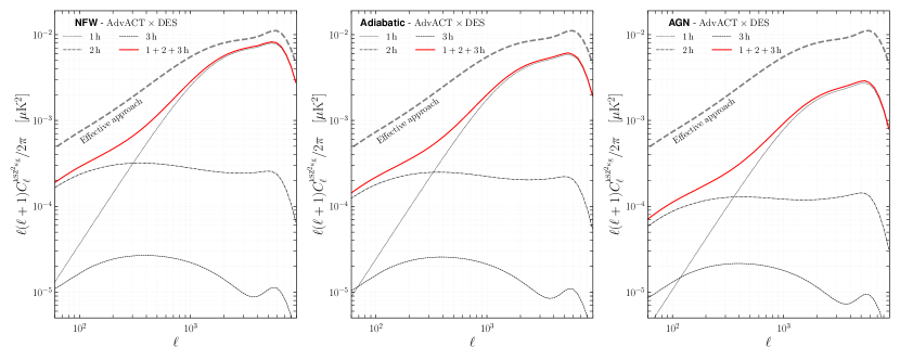
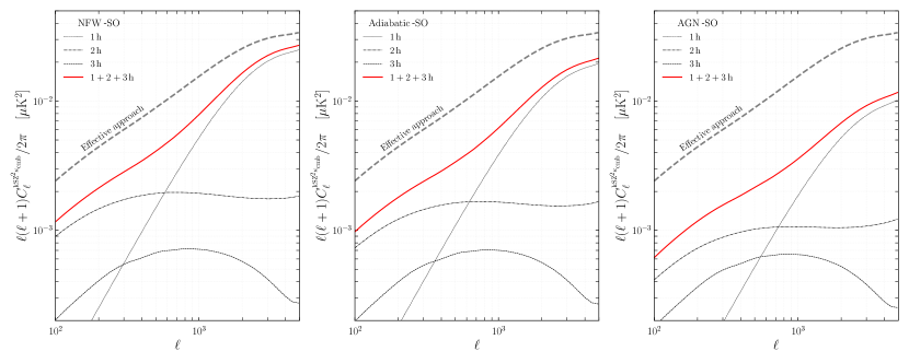
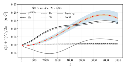
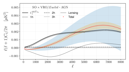
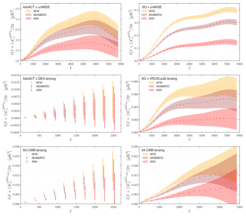
We validate the class_sz implementation of the effective approach against the code used in Hill et al. (2016); Ferraro et al. (2016); Kusiak et al. (2021) by comparing the predictions of both codes, in two cases. For both cases (Planck $\times$ WISE and AdvACT $\times$ WISE), the codes agree within $\approx 10\%$ (see Appendix C.2 and Figure 21). For the experimental configurations and cross-correlations of interest here, we show the effective approach projected-field kSZ power spectrum in Figures 5, 6, and 7 as the thick dashed lines.

The main limitations of the effective approach are its range of validity and its range of applications. It is well established that the gas in the ICM and CGM does not follow the underlying dark matter density profile (e.g., Schaan et al., 2021), because of energetic feedback mechanisms or clusters’ formation history. Therefore, the assumption $\delta_{\mathrm{e}}=f_{\mathrm{b}}f_{\mathrm{free}}\delta_{\mathrm{m}}$ is not a valid assumption in the high-$k$ regime, within halos. In addition, due to that same assumption, the effective approach does not enable us to probe the scale dependence of the gas density profile. By relaxing this assumption and using physical models for the gas distribution, the halo model allows us to overcome these limitations.

Figure 4: Left: The mass of the gas (baryons) enclosed within a radius $r=xr_{\mathrm{200c}}$ for three different profile shapes. NFW is the standard NFW formula, while Adiabatic and AGN are the models of Table 2. The halo has a mass $m_{\mathrm{200c}}=3.3\times 10^{13}\,M_{\odot}$ and is at $z=0.55$. The vertical lines indicate the truncation radius for the Adiabatic and AGN profiles. They are such that the enclosed mass is $m_{\mathrm{200c}}$. The horizontal line indicates the gas mass of the halo, namely $f_{\mathrm{b}}\times 3.3\,M_{\odot}\simeq 3.5\times 10^{12}\,M_{\odot}/h$. Right: Same as left but showing the scaled gas density. The critical density of the denominator of the $y$-axis label is evaluated at redshift $z$. The shaded area under the curves indicate the region below the truncation radius (vertical lines in the left plot). Other cosmological and halo model settings are set to our fiducial model (see Section 2.1).

3 Halo Model

In this Section we describe the halo model approach. In Subsection 3.2 we use the halo model (e.g., Scherrer & Bertschinger, 1991; Mo & White, 1996; Scoccimarro et al., 2001; Seljak, 2000; Cooray & Sheth, 2002) to estimate the hybrid bispectrum $B_{\delta_{\mathrm{e}}\delta_{\mathrm{e}}X}$ (Eq. (32)) and describe our two gas density profile parameterization choices. In Subsection 3.4 we explain how to compute the projected-field kSZ power spectrum with the halo model hybrid bispectrum.

3.1 The Halo Model Code: class_sz

Along with this paper, we release version v1 of the halo model code class_sz. The code is written in C and was originally developed by Bolliet et al. (2018), specifically for the calculation of the thermal SZ power spectrum within the halo model and based on the Fortran code szfastdks (Komatsu & Seljak, 2002; Dolag et al., 2016). We have extended it to enable the calculation of power spectra and bispectra of most LSS tracers, including galaxy number density, galaxy weak lensing, CMB weak lensing, the cosmic infrared background (CIB), and the kSZ effect.

Version v1 of class_sz is built onto version v2.9.4 of the class code (Lesgourgues, 2011; Blas et al., 2011). This approach has two main advantages. First, with class_sz, one can compute all the quantities available in class such as the CMB temperature and polarization anisotropy power spectra or the matter power spectrum. Second, this makes most of the halo model quantities in class_sz computable within all the cosmological models implemented in class. The class_sz code performs fast and accurate evaluations of the redshift and mass integrals (see Eq. 1 and 2 hereafter) in the halo model using an adaptive Patterson scheme (Patterson, 1968) imported from CosmoTherm (Chluba & Sunyaev, 2011). Where possible, the code’s outputs have been checked with other halo-model codes, including ccl (Chisari et al., 2019), yxg (Koukoufilippas et al., 2020), hmvec (Smith et al., 2018), and HaloGen (Schaan et al., 2018). Compared to other halo model codes, class_sz has the unique property of full integration with class and follows the same computational strategy as class for the halo model quantities.

The class_sz code computes power spectra $P(k)$, bispectra $B(k,k^{\prime},k^{\prime\prime})$, and angular power spectra $C_{\ell}$ within the Limber approximation (see Eq. 3) on the flat sky. These calculations are parallelized in a similar way as the transfer function calculations in the original class code. In particular, each $k$- or $\ell$-mode of a given power spectrum or bispectrum, which requires its own redshift and mass integral, is computed by a single thread. Hence, the evaluation time of a typical calculation will generally benefit from setting the OpenMP environment variable OMP_NUM_THREADS to the highest possible value given the computing platform architecture. Quantities that are common to most $k$- and $\ell$-mode integrands, and which are computationally expensive, are pre-tabulated outside of the main parallel block. The tabulations themselves are parallelized, e.g., over a redshift and mass grid, when possible.

The code borrows special functions and an integrator for oscillatory functions from gsl (Galassi, 2018), interpolation and root finding routines from J. Burkardt’s scientific library, and the FFTLog algorithm (Hamilton, 2000) as implemented by A. Slosar. Hence, in addition to the dependencies of the class code, class_sz requires gsl and FFTW3 (Frigo & Johnson, 2005), properly installed and linked.

The python wrapper classy_sz can be called within any Python code. In particular, classy_sz is easily interfaced with Markov Chain Monte Carlo (MCMC) samplers such as MontePython (Brinckmann & Lesgourgues, 2018; Audren et al., 2013) and Cobaya (Torrado & Lewis, 2021) for Bayesian inference, as well as machine learning packages such as CosmoPower (Mancini et al., 2022).

3.2 Halo Model for the Hybrid Bispectrum

The hybrid bispectrum, introduced in Eq. (31-32), is defined by

$$\langle\delta_{\mathrm{e}}(\bm{k}_{1})\delta_{\mathrm{e}}(\bm{k}_{2})X(\bm{k}_{3})\rangle=(2\pi)^{3}\delta_{D}(\bm{k}_{1}+\bm{k}_{2}+\bm{k}_{3})B_{\delta_{\mathrm{e}}\delta_{\mathrm{e}}X}(k_{1},k_{2},k_{3}),$$ (38)

where $\delta_{\mathrm{e}}$ is the electron density perturbation and $X$ is to be understood as the perturbation in the tracer field. In the halo model, the hybrid bispectrum is the sum of three terms

$$B_{\delta_{\mathrm{e}}\delta_{\mathrm{e}}X}=B_{\delta_{\mathrm{e}}\delta_{\mathrm{e}}X}^{\mathrm{1h}}+B_{\delta_{\mathrm{e}}\delta_{\mathrm{e}}X}^{\mathrm{2h}}+B_{\delta_{\mathrm{e}}\delta_{\mathrm{e}}X}^{\mathrm{3h}},$$ (39)

where the one-halo (1h) term corresponds to three points within the same halo, the two-halo term (2h) to three points within two halos, and the three-halo term (3h) to three points in three distinct halos (see, e.g., Ma & Fry, 2000; Scoccimarro et al., 2001; Valageas & Nishimichi, 2011; Lacasa et al., 2014; Lazanu et al., 2016, for further details on halo model bispectra). Then, each term is expressed in terms of ensemble averages over halos as (at a given redshift/comoving distance):

$$B_{\delta_{\mathrm{e}}\delta_{\mathrm{e}}X}^{\mathrm{1h}} =\int\mathrm{d}n_{1}\hat{u}_{k_{1}}^{\mathrm{e}}(m_{1})\hat{u}_{k_{2}}^{\mathrm{e}}(m_{1})\hat{u}_{k_{3}}^{X}(m_{1})$$ (40)

$$B_{\delta_{\mathrm{e}}\delta_{\mathrm{e}}X}^{\mathrm{2h}} =\int\mathrm{d}n_{1}b^{(1)}(m_{1})\hat{u}_{k_{1}}^{\mathrm{e}}(m_{1})\hat{u}_{k_{2}}^{\mathrm{e}}(m_{1})\int\mathrm{d}n_{2}b^{(1)}(m_{2})\hat{u}_{k_{3}}^{X}(m_{2})P_{L}(k_{3})+\mathrm{perms}$$ (41)

$$B_{\delta_{\mathrm{e}}\delta_{\mathrm{e}}X}^{\mathrm{3h}} =2\int\mathrm{d}n_{1}b^{(1)}(m_{1})\hat{u}_{k_{1}}^{\mathrm{e}}(m_{1})P_{L}(k_{1})\int\mathrm{d}n_{2}b^{(1)}(m_{2})\hat{u}_{k_{2}}^{\mathrm{e}}(m_{2})P_{L}(k_{2})\int\mathrm{d}n_{3}b^{(1)}(m_{3})\hat{u}_{k_{3}}^{X}(m_{3})F_{2}(k_{1},k_{2},k_{3})$$

$$+\int\mathrm{d}n_{1}b^{(1)}(m_{1})\hat{u}_{k_{1}}^{\mathrm{e}}(m_{1})P_{L}(k_{1})\int\mathrm{d}n_{2}b^{(1)}(m_{2})\hat{u}_{k_{2}}^{\mathrm{e}}(m_{2})P_{L}(k_{2})\int\mathrm{d}n_{3}b^{(2)}(m_{3})\hat{u}_{k_{3}}^{X}(m_{3})+\mathrm{perms}$$ (42)

where we did not write explicitly the permutations (see Appendix B.4 for details) and where $F_{2}$ is the kernel defined in Eq. (34) for the tree-level bispectrum. Here, $\hat{u}_{k}^{\mathrm{e}}(m)$ is the Fourier transform of the gas density profile (divided by $\rho_{\mathrm{m,0}}$, see below) and $\hat{u}_{k}^{X}(m)$ is the Fourier transform of the radial profile of $X$, e.g., the mass profile for weak lensing fields, or the galaxy HOD for galaxy density.

With $\delta_{\mathrm{e}}=X=\delta_{\mathrm{m}}$, this formula reduces to the halo model matter bispectrum (see, e.g., Section IV.A of Lazanu et al., 2016), which we plot in Figure 3 (top row). We refer to Lazanu et al. (2017) and Philcox et al. (2020) for a discussion on the accuracy of the halo model expressions and possible extensions.

3.3 Gas Density Profile

For the gas density profile, $\rho_{\mathrm{gas,free}}$, we consider two parameterizations. First, the NFW formula (Navarro et al., 1997) rescaled by the baryon fraction $f_{\mathrm{b}}$, i.e.,

$$\rho_{\mathrm{gas,free}}(r)=f_{\mathrm{b}}f_{\mathrm{free}}\rho_{{}_{\mathrm{NFW}}}(r)$$ (43)

where $\rho_{{}_{\mathrm{NFW}}}(r)$ is the usual NFW profile (see Appendix B.9 for details). Second, a generalized NFW (gNFW) formula, following Battaglia (2016):

$$\rho_{\mathrm{gas,free}}(r)=f_{\mathrm{b}}f_{\mathrm{free}}\rho_{\mathrm{crit}}(z)C\left(\frac{r}{x_{\mathrm{c}}r_{\mathrm{200c}}}\right)^{\gamma}\left[1+\left(\frac{r}{x_{\mathrm{c}}r_{\mathrm{200c}}}\right)^{\alpha}\right]^{-\frac{\beta+\gamma}{\alpha}},$$ (44)

where $r_{\mathrm{200c}}$ is the characteristic radius associated with the overdensity mass $m_{\mathrm{200c}}$ (see Eq. B22), with $x_{c}=0.5$ and $\gamma=-0.2$ kept fixed throughout the paper and with mass and redshift dependent parameters $C,\alpha,\beta,\gamma$, such that

$$p=A_{0}\left(\frac{m_{\mathrm{200c}}}{10^{14}M_{\odot}}\right)^{A_{m}}\left(1+z\right)^{A_{z}}\quad\mathrm{for}\quad p\in\{C,\alpha,\beta,\gamma\}.$$ (45)

For $A_{0},A_{m},A_{z}$ we use the best-fit values from Battaglia (2016) reported in Table 2, corresponding to either the AGN feedback model (that is our fiducial assumption) or the Adiabatic model. Note that the NFW profile is a subcase of the gNFW formula, when parameters are set to $x_{c}=1/c_{200c}$, $\gamma=-1$, $\alpha=1$, $\beta=3$, and $C=\rho_{s}/\rho_{\mathrm{crit}}(z)$, where $c_{200c}$ is the concentration computed with the Bhattacharya et al. (2013) relation and $\rho_{s}$ is the normalization of the NFW profile defined in Eq. (B23).

	AGN feedback			Adiabatic
$p$	$A_{0}$	$A_{m}$	$A_{z}$	$A_{0}$	$A_{m}$	$A_{z}$
$C$	$4\times 10^{3}$	$0.29$	$-0.66$	$1.9\times 10^{4}$	$0.09$	$-0.95$
$\alpha$	$0.88$	$-0.03$	$0.19$	$0.70$	$-0.017$	$0.27$
$\beta$	$3.83$	$0.04$	$-0.025$	$4.43$	$0.005$	$0.037$

Table 2: Best-fit values of the parameters of the generalized NFW gas density profile formula fit to simulations from Battaglia (2016). Adiabatic corresponds to simulations whose sub-grid model has only gravitational heating. AGN feedback corresponds to a sub-grid model with radiative cooling, star formation, supernova feedback, cosmic rays, and AGN feedback. The gas density profile is computed using these parameters in Eq. (44). (See Battaglia, 2016, for details.)

With this, we compute the Fourier transforms entering Eqs. (40-42) as

$$\hat{u}^{\mathrm{e}}_{k}=4\pi\int_{0}^{\infty}\mathrm{d}rr^{2}j_{0}(kr)\mathrm{H}(r_{\mathrm{cut}}-r)u^{\mathrm{e}}(r)\quad\mathrm{with}\quad j_{0}(x)=\frac{\sin(x)}{x}\quad\mathrm{and}\quad u^{\mathrm{e}}(r)=\frac{\rho_{\mathrm{gas,free}}(r)}{\rho_{\mathrm{m,0}}},$$ (46)

where $\mathrm{H}$ is the Heaviside step function (which truncates the profile at $r_{\mathrm{cut}}$) and where we used the fact that the profiles are radially symmetric to write the Fourier transform as a Hankel transform. In general, it is necessary to truncate the density profiles because their volume integrals do not converge or may have support at unphysically large radii. For the NFW profile, we set the truncation radius to $r_{\mathrm{cut}}=r_{\mathrm{200c}}$. For the gNFW profile we require $r_{\mathrm{cut}}$ to be such that the enclosed gas mass is the same as in the NFW case, i.e., $f_{\mathrm{b}}m_{200c}$. We then find $r_{\mathrm{cut}}$ numerically with Brent’s method (Brent, 1973), solving

$$F(r_{\mathrm{out}};m_{\mathrm{200c}},z)=0\quad\mathrm{with}\quad F(r_{\mathrm{out}};m_{\mathrm{200c}},z)=4\pi\int_{0}^{\mathrm{r_{\mathrm{cut}}}}\mathrm{d}rr^{2}\rho_{\mathrm{gas}}(r;m_{\mathrm{200c}},z)-f_{\mathrm{b}}m_{\mathrm{200c}},$$ (47)

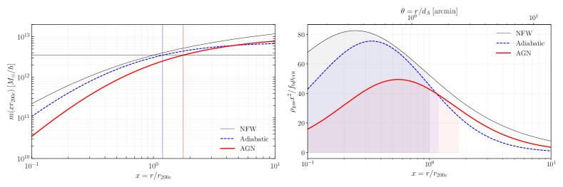
where we wrote the mass and redshift dependence explicitly to emphasize the fact that this operation is done at each mass and redshift. The left panel of Figure 4 illustrates the method. It shows the enclosed gas mass as a function of radius (in units of $r_{\mathrm{200c}}$). The horizontal line indicates the gas mass of the halo, namely $f_{\mathrm{b}}\times 3.3\,M_{\odot}$. By definition, it intersects the NFW curve at $r_{\mathrm{200c}}$, i.e., $x=1$. The blue and red vertical lines represent the truncation radii as obtained by solving Eq. (47), and consistently intersect the Adiabiatic and AGN curves at $f_{\mathrm{b}}\times 3.3\,M_{\odot}$. The right panel of Figure 4 compares the NFW, Adiabatic and AGN profiles (rescaled by $x^{2}/f_{\mathrm{b}}\rho_{\mathrm{crit}}$). The area below each curve (which is proportional to the mass) is colored for $x$ corresponding to $r<r_{\mathrm{cut}}$.

We note that halo models based on the Battaglia (2016) gas density profile parameterization have been used in multiple previous analyses (e.g., Smith et al., 2018; Münchmeyer et al., 2019; Cayuso et al., 2021; Roy et al., 2022), which computed Fourier and harmonic space two-point functions. In principle, our results could be checked against these studies. One notable difference is that previous works often truncate the gas density profile at $r_{\mathrm{200c}}$, and rescale its amplitude by a factor such that the enclosed mass is $m_{\mathrm{200c}}$. We argue that our truncation method is more consistent, as it preserves the total gas mass but does not alter the density as a function of radius.

In Figure 3, we show the matter hybrid bispectrum for $kSZ^{2}\times\delta_{\mathrm{g}}$ cross-correlation at $z=1$ computed according to the different approaches discussed above. We show three different triangle configurations, parameterized via $(k,k^{\prime},k^{\prime\prime})=(k,\lambda k,\lambda^{\prime}k)$, with $\lambda=\lambda^{\prime}=1$ for the Equilateral configuration, $\lambda=1,\lambda^{\prime}=0.1$ for the Squeezed configuration and $\lambda=0.5,\lambda^{\prime}=0.5$ for the Flattened configuration. For the hybrid bispectrum, we show the dimensionless combinations $b_{\mathrm{g}}(z)W^{\mathrm{kSZ}}(\chi)^{2}f_{\mathrm{b}}^{2}f_{\mathrm{free}}^{2}B_{\mathrm{TL}}$ for the Tree-Level line, $b_{\mathrm{g}}(z)W^{\mathrm{kSZ}}(\chi)^{2}f_{\mathrm{b}}^{2}f_{\mathrm{free}}^{2}B_{\mathrm{eff}}^{NL}$ for the effective approach lines (where $b_{\mathrm{g}}(z)$ is given in Eq. B29), and $W^{\mathrm{kSZ}}(\chi)^{2}B_{\delta_{\mathrm{e}}\delta_{\mathrm{e}}\delta_{\mathrm{g}}}^{i\mathrm{h}}$ with $i=1,2,3$ for the halo-model lines (see Eq. 40-42).

Figure 5: (Galaxy density) Projected-field kSZ power spectrum in cross-correlation with galaxies, assuming our fiducial model (see Section 2.1). The halo model predictions (Section 3) are the thick red lines and thin dashed and dotted lines. The top row shows the three different profiles, i.e., NFW, Adiabatic, and AGN Feedback (see Table 2 and Eq. 44) assuming a Planck CMB map and the bottom row shows the same but assuming an AdvACT CMB map (see Table 1). The effective approach predictions (Subsection 2.4) are the grey dashed lines – they do not change from column to column. Furthermore, they are multiplied by the redshift dependent bias $b_{\mathrm{g}}(z)$ of Eq. B29. The galaxy HOD parameters are for an unWISE-like catalogue and are given below Eq. B29. The overall signal is much larger in the bottom row because the AdvACT filter preserves much more of the small-scale kSZ signal than that of Planck (see Figure 2).

Figure 6: (Galaxy lensing) Projected-field kSZ power spectrum in cross-correlation with galaxy lensing, assuming our fiducial model (see Section 2.1). The effective approach prediction (see Subsection 2.4) is the thick dashed line and is the same in each panel. The halo model predictions (Section 3) are the thick red lines and thin dashed and dotted lines. Each panel shows a different profile, i.e., NFW, Adiabatic, and AGN Feedback (from left to right – see Table 2 and Eq. 44), and they all assume an AdvACT CMB map (see Table 1). For galaxy weak lensing we assume a DES-like survey (see Table 3).

Figure 7: (CMB lensing) Projected-field kSZ power spectrum in cross-correlation with CMB lensing, assuming our fiducial model (see Section 2.1). The effective approach prediction (see Subsection 2.4) is the thick dashed line and is the same in each panel. The halo model predictions (Section 3) are the thick red lines and thin dashed and dotted lines. Each panel shows a different profile, i.e., NFW, Adiabatic, and AGN Feedback (from left to right – see Table 2 and Eq. 44), and they all assume an SO CMB map (see Table 1). For CMB weak lensing we assume an SO map as well (see Table 3).

3.4 The Projected-field kSZ Power Spectrum and its Numerical Implementation

To compute the projected-field kSZ power spectrum with the halo model, we use Eq. (32) where we replace $B_{\delta_{\mathrm{e}}\delta_{\mathrm{e}}X}$ by the halo model hybrid bispectrum discussed in the previous section. The three terms of the halo model hybrid bispectrum (see Eq. 40-42) yield three terms for the projected-field kSZ power spectrum, which we can write as

$$C_{\ell}^{\mathrm{kSZ}^{2}X}=C_{\ell}^{\mathrm{kSZ}^{2}X,1\mathrm{h}}+C_{\ell}^{\mathrm{kSZ}^{2}X,2\mathrm{h}}+C_{\ell}^{\mathrm{kSZ}^{2}X,3\mathrm{h}}.$$ (48)

At this point, we know how to compute the halo model projected-field kSZ power spectrum. The challenge is to find an efficient numerical implementation. The most straightforward option is to carry out the multiple integrals one after the other, as we described for the effective approach implementation (see Subsection 2.4). The difference is that the halo model hybrid bispectrum requires integration over halo mass. Hence for the one-halo term, we need to compute a four-dimensional integral (over redshift, $\ln\ell^{\prime}$, $\theta$ and $m_{1}$), for the two-halo term a five-dimensional integral (same as one-halo, plus $m_{2}$ integral) and for the three-halo term a six-dimensional integral (same as for the two-halo term, plus $m_{3}$ integral). This is numerically tractable, however the computation is time-consuming, taking $\sim\mathcal{O}(10^{3}\mathrm{s})$ on a laptop.

Fortunately, there exists a way to accelerate the computation because the halo model enables us to take a shortcut when evaluating the 2D integral over $\bm{\ell}^{\prime}$ in Eq. (32). It relies on the fact that the halo model hybrid bispectrum terms are all separable with respect to scale/wavenumber. Hence, the triangle power spectrum (Eq. 32) is a 2D convolution which can be evaluated rapidly using the FFTLog algorithm (Hamilton, 2000). Let us describe the procedure in more detail. Starting from Eq. (32), we first split the triangle power spectrum into the three halo-model terms and treat them separately: $T(\ell,\chi)=T^{\mathrm{1h}}(\ell,\chi)+T^{\mathrm{2h}}(\ell,\chi)+T^{\mathrm{3h}}(\ell,\chi)$. Using the expression of the one-halo term of the hybrid bispectrum (Eq. 40) and re-arranging, we can write the one-halo term of the triangle power spectrum as

$$T^{\mathrm{1h}}(\ell,\chi)=\frac{1}{(2\pi)^{2}}\int\mathrm{d}n\hat{u}^{X}_{\ell}\int\mathrm{d}^{2}\bm{\ell}^{\prime}\left[w(\ell^{\prime})\hat{u}^{\mathrm{e}}_{\ell^{\prime}}\right]\left[w(\left|\bm{\ell}+\bm{\ell}^{\prime}\right|)\hat{u}^{\mathrm{e}}_{|\bm{\ell}+\bm{\ell}^{\prime}|}\right].$$ (49)

From the convolution theorem, we can replace the integral over $\mathrm{d}^{2}\bm{\ell}^{\prime}$ by Fourier transform operations as

$$T^{\mathrm{1h}}(\ell,\chi)=\frac{1}{(2\pi)^{2}}\langle\hat{u}^{X}_{\ell}\varphi(\ell)\rangle_{n},\quad\mathrm{with}\quad\varphi^{\mathrm{1h}}\equiv\mathcal{F}^{-1}\left\{\mathcal{F}\left\{w\hat{u}^{\mathrm{e}}\right\}\cdot\mathcal{F}\left\{w\hat{u}^{\mathrm{e}}\right\}\right\},$$ (50)

where $\mathcal{F}$ is the Fourier transform (from harmonic space to angular space), and $\mathcal{F}^{-1}$ is its inverse. Note that here, the Fourier transform operations are performed inside the mass integral (the integral over $\mathrm{d}n$, denoted $\langle\cdots\rangle_{n}$). Eventually, we integrate over redshift to get $C_{\ell}^{\mathrm{kSZ}^{2}X,1\mathrm{h}}$.

For the two-halo term, there are two mass integrals. Moreover, due to the cyclic permutation we have three terms to deal with. For one of these terms, which we denote $T_{\mathrm{tog.}}^{\mathrm{2h}}$ , we have two $\hat{u}^{\mathrm{e}}$’s within the same mass integral. For the other two terms, each $\hat{u}^{\mathrm{e}}$ is in a separate mass integral, and we denote their sum $T_{\mathrm{sep.}}^{\mathrm{2h}}$. In fact, both terms in $T_{\mathrm{sep.}}^{\mathrm{2h}}$ contribute equally, because of the invariance of the expression under the transformation $\ell\leftrightarrow|\bm{\ell}+\bm{\ell}^{\prime}|$.

Using the expression of the two-halo term of the hybrid bispectrum (Eq. 41), and re-arranging, we get

$$T^{\mathrm{2h}}_{\mathrm{tog.}}(\ell,\chi) =\frac{1}{(2\pi)^{2}}\langle b^{(1)}\varphi^{\mathrm{2h}}_{\mathrm{tog.}}(\ell)\rangle_{n}\langle b^{(1)}\hat{u}^{X}_{\ell}\rangle_{n}P_{L},\quad\mathrm{with}\quad\varphi^{\mathrm{2h}}_{\mathrm{tog.}}\equiv\mathcal{F}^{-1}\left\{\mathcal{F}\left\{w\hat{u}^{\mathrm{e}}\right\}\cdot\mathcal{F}\left\{w\hat{u}^{\mathrm{e}}\right\}\right\},$$ (51)

$$T^{\mathrm{2h}}_{\mathrm{sep.}}(\ell,\chi) =\frac{1}{2\pi^{2}}\varphi^{\mathrm{2h}}_{\mathrm{sep.}}(\ell),\quad\mathrm{with}\quad\varphi^{\mathrm{2h}}_{\mathrm{sep.}}\equiv\mathcal{F}^{-1}\{\mathcal{F}\{w\langle b^{(1)}\hat{u}^{\mathrm{e}}\rangle_{n}P_{L}\}\cdot\mathcal{F}\{w\langle b^{(1)}\hat{u}^{\mathrm{e}}\hat{u}^{X}_{\ell}\rangle_{n}\}\},$$ (52)

where $P_{L}$ in Eq. (51) is evaluated at $k=(\ell+1/2)/\chi$. Note that, as for the one-halo term, the Fourier transform operations in Eq. (51) are carried out inside the mass integral, while in Eq. (52) the Fourier transform operations are carried out after the mass integrals. Then we have $T^{\mathrm{2h}}=T^{\mathrm{2h}}_{\mathrm{tog.}}+T^{\mathrm{2h}}_{\mathrm{sep.}}$, which we can integrate over redshift according to Eq. (32) to get $C_{\ell}^{\mathrm{kSZ}^{2}X,2\mathrm{h}}$.

For the three-halo term, let us first notice that the hybrid bispectrum splits into terms proportional to the second order bias $b^{(2)}$ and terms proportional to the $F_{2}$-kernel (see Eq. 42). Hence, for the triangle power spectrum we have $T^{\mathrm{3h}}=T^{\mathrm{3h}}_{b^{(2)}}+T^{\mathrm{3h}}_{F_{2}}$. Accounting for permutations, there are three terms proportional to $b^{(2)}$ in the hybrid bispectrum, but two of them contribute equally to $T^{\mathrm{3h}}_{b^{(2)}}$ due to the symmetry $\ell\leftrightarrow|\bm{\ell}+\bm{\ell}^{\prime}|$. After re-arranging we get

$$T_{b^{(2)}}^{\mathrm{3h}}(\ell,\chi)=\frac{1}{(2\pi)^{2}}\varphi^{\mathrm{3h,1}}_{b^{(2)}}\langle b^{(2)}\hat{u}^{X}_{\ell}\rangle_{n}+\frac{1}{2\pi^{2}}\varphi^{\mathrm{3h,2}}_{b^{(2)}}\langle b^{(1)}\hat{u}^{X}_{\ell}\rangle_{n}P_{L},$$ (53)

where here $P_{L}$ is evaluated at $k=(\ell+1/2)/\chi$ and where we introduced the definitions

$$\varphi^{\mathrm{3h,1}}_{b^{(2)}}\equiv\mathcal{F}^{-1}\{\mathcal{F}\{w\langle b^{(1)}\hat{u}^{\mathrm{e}}\rangle_{n}P_{L}\}\cdot\mathcal{F}\{w\langle b^{(1)}\hat{u}^{\mathrm{e}}\rangle_{n}P_{L}\}\}\quad\mathrm{and}\quad\varphi^{\mathrm{3h,2}}_{b^{(2)}}\equiv\mathcal{F}^{-1}\{\mathcal{F}\{w\langle b^{(1)}\hat{u}^{\mathrm{e}}\rangle_{n}\}\cdot\mathcal{F}\{w\langle b^{(2)}\hat{u}^{\mathrm{e}}\rangle_{n}P_{L}\}\}.$$ (54)

Note that here, the Fourier transform operations are carried out after the mass integrals.

To compute $T^{\mathrm{3h}}_{F_{2}}$, we start by expanding $F_{2}$ as

$$F_{2}(k_{1},k_{2},k_{3})=\frac{5}{14}+\frac{3}{28}x_{31}^{2}+\frac{3}{28}x_{32}^{2}-\frac{5}{28}x_{12}^{2}-\frac{5}{28}x_{21}^{2}+\frac{1}{14}x_{31}^{2}x_{32}^{2}\quad\mathrm{with}\quad x_{ij}\equiv k_{i}/k_{j},\,\,i,j\in\{1,2,3\}$$ (55)

Since this form of $F_{2}$ has six terms and accounting for the cyclic permutation, we can write the hybrid bispectrum terms proportional to $F_{2}$ as a sum of eighteen terms, namely

$$B^{\mathrm{3h}}_{F_{2}}=\sum_{i=1}^{18}\omega_{i}\left[\langle b^{(1)}\hat{u}^{\mathrm{e}}_{k_{1}}\rangle_{n}P_{L}(k_{1})^{s}k_{1}^{p}\right]\left[\langle b^{(1)}\hat{u}^{\mathrm{e}}_{k_{2}}\rangle_{n}P_{L}(k_{2})^{t}k_{2}^{q}\right]\left[\langle b^{(1)}\hat{u}^{X}_{k_{3}}\rangle_{n}P_{L}(k_{3})^{u}k_{3}^{r}\right]$$ (56)

where $\omega_{i}$ are rational prefactors determined by the prefactors in Eq. (55), where $p,q,r\in\{0,2,-2,4\}$ such that $p+q+r=0$ and where $s,t,u\in\{0,1\}$ such that $s+t+u=2$. (The combination of indices $p,q,r,s,t,u$ is different for each of the 18 terms.) Here we used wavenumbers rather than multipoles — we assume the same correspondence as in Eq. (32). Due to the symmetry $\ell\leftrightarrow|\bm{\ell}+\bm{\ell}^{\prime}|$, these eighteen terms yield ten different terms in $T^{\mathrm{3h}}_{F_{2}}$ (twelve of the eighteen terms contribute equally). After re-arranging, we get

$$T_{F_{2}}^{\mathrm{3h}}(\ell,\chi)=\frac{1}{(2\pi)^{2}}\sum_{i=1}^{10}c_{i}\mathcal{F}^{-1}\left\{\mathcal{F}\{w\langle b^{(1)}\hat{u}^{\mathrm{e}}\rangle_{n}P_{L}(k)^{s}k^{p}\}\cdot\mathcal{F}\{w\langle b^{(1)}\hat{u}^{\mathrm{e}}\rangle_{n}P_{L}(k)^{t}k^{q}\}\right\}\left[\langle b^{(1)}\hat{u}^{X}_{k_{3}}\rangle_{n}P_{L}(k_{3})^{u}k_{3}^{r}\right]$$ (57)

where $k_{3}=(\ell+1/2)/\chi$ and where $c_{i}$ are numerical constants, $c_{1}=c_{5}=5/7,c_{2}=2c_{8}=2c_{9}=-5/7,c_{3}=2c_{6}=2c_{7}=3/7,c_{4}=c_{10}=1/7$, with $(u,s,t)=(0,1,1)$ for $1\leq i\leq 4$ and $(u,s,t)=(1,1,0)$ for $5\leq i\leq 10$. Eventually, we obtain $C_{\ell}^{\mathrm{kSZ}^{2}X,\mathrm{3h}}$ by summing Eqs. (53) and (57), and integrating over redshift according to Eq. (32).

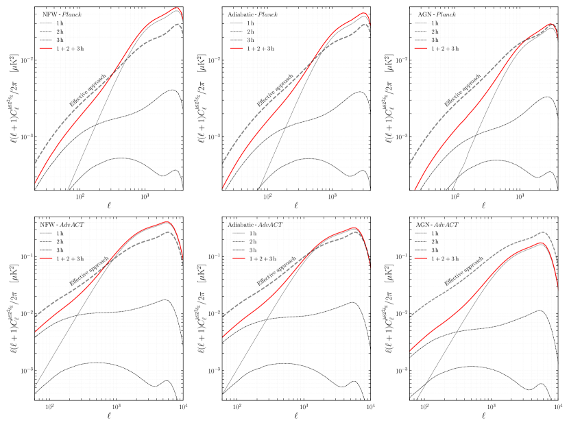
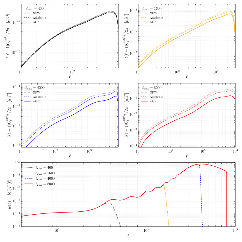
The halo model prediction is shown in detail in Figures 5, 6 and 7, where we plot it against the effective approach prediction. Naively, one would expect that on large scales the projected-field power spectrum should always hold to the same limit, irrespective of gas profile assumptions (determined by the fact that the enclosed mass is always the same). However, in our case it is not true because of the convolution which mixes contributions from all scales at each $\ell$ (see Eq. (28)). One way to recover the intuitive large-scale behavior is to artificially filter out the small scales.

In Figure 8, we show the halo model kSZ²-galaxy projected-field power spectrum computed without contributions from small scales. We remove the small-scale contributions by defining a filter in harmonic space which vanishes for $\ell>\ell_{\mathrm{max}}$, using the taper function of footnote 5. The filters (multiplied by the beam) are shown on the same plot in the bottom panel. The top panels are the resulting power spectra for four different values of $\ell_{\mathrm{max}}$ between 400 and 8000. We see that for $\ell_{\mathrm{max}}=8000$ and 4000, the different density profile assumptions (NFW, Adiabatic, and AGN) are easily distinguishable since the amplitudes of the power spectra significantly differ. However, for $\ell_{\mathrm{max}}=1600$ the difference is smaller and for $\ell_{\mathrm{max}}=400$ the three profile assumptions yield nearly the same projected-field power spectrum. The fact that the power spectra converge to the same amplitude is a good sanity check. It shows that our implementation is consistent with the fact that on large scales the projected-field power spectrum is sensitive to the overall gas mass rather than the details of the shape of the profiles. Although this figure shows results only for the kSZ²–galaxy cross-correlation, we expect the same results for other LSS tracers.

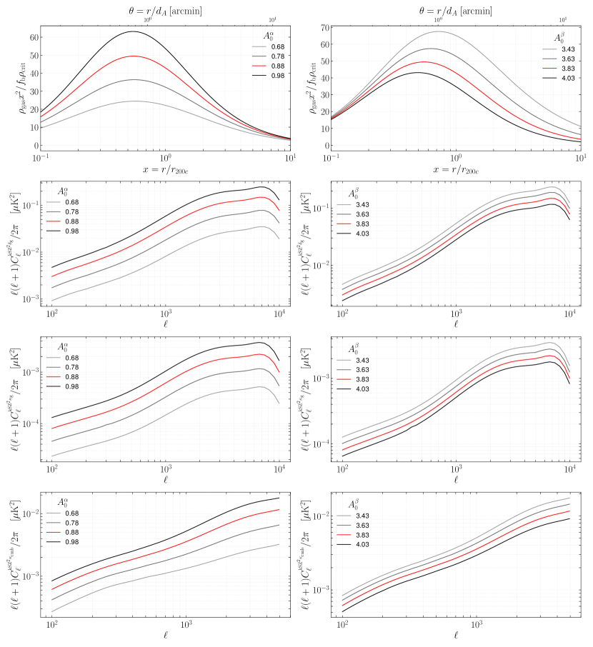
The halo-model implementation allows us to study the projected-field power spectrum for arbitrary shapes of the gas density profile beyond the AGN, Adiabatic, and NFW models. In this paper we implement the gNFW formula from Battaglia (2016). (Of course, one could easily extend our implementation to other gas models.) Thus, we can study the projected-field power spectrum predictions for different values of the parameters entering the gNFW formula. In the top row of Figure 9, we consider the same dark matter halo as in Figure 4, i.e., with a mass of $3.3\times 10^{13}\,M_{\odot}$ at $z=0.55$, and show the scaled density profile for different values of the slope parameters $\alpha$ and $\beta$ around the fiducial AGN model (red line). In the formalism of Battaglia (2016) these slope parameters have a mass and redshift dependence. Here, for simplicity, we keep the mass and redshift dependence fixed to the fiducial AGN feedback values, and only change the overall amplitude determined by $A_{0}^{\alpha}$ and $A_{0}^{\beta}$. On the left plot, we see that $\alpha$ mainly determines the gas density in the inner part of the halo — $\alpha$ is referred to as the inner slope. On the right plot we see that $\beta$ mainly determines the gas density in the outer part of the profile — $\beta$ is referred to as the outer slope. In the bottom rows of Figure 9, we show the projected-field power spectrum predictions associated with these different gas density profiles determined by the specific values of $A_{0}^{\alpha}$ and $A_{0}^{\beta}$. The fiducial AGN feedback predictions are shown in red and each row corresponds to a different LSS tracer: galaxies (second row), galaxy lensing (third row), and CMB weak lensing (fourth row). The same conclusion holds in all cases: changing the gas profile shape appears to amount to an overall shift of the projected-field power spectrum. This behavior differs from what is obtained for the kSZ power spectrum, where different gas density profiles yield the same large-scale power (see Figure 18). Again, it is due to the fact that in the projected-field estimator, small scales (sensitive to the gas profile shape rather than the integrated mass) contribute at all multipoles including the low-$\ell$ part, because of the convolution of the profiles in harmonic space (see Eq. (28)). This is entirely due to the “squaring operation” on the CMB map, irrespective of the LSS tracer, as illustrated in the figure.

Figure 8: Projected-field kSZ power spectrum in cross-correlation with galaxy number density (assuming the case of unWISE galaxies, see Table 3). Here, we assume an SO-like CMB map (see Table 1). The bottom panel shows four filter choices with different $\ell_{\mathrm{max}}$ (multiplied by the beam — see Eq. 27). The top panels show the corresponding predictions for the projected-field power spectrum. Each of the top panels shows the three different gas profile assumptions: NFW, Adiabatic, and AGN Feedback (see Table 2 and Eq. 44). This figure illustrates that when small scales are removed (case $\ell_{\mathrm{max}}=400$), the three different profile assumptions become almost indistinguishable.

Figure 9: Radial gas density profile (top row) for the same dark matter halo as in Figure 4 and projected-field kSZ power spectrum predictions for different values of the inner slope parameter $\alpha$ (left) and outer slope parameter $\beta$ (right). See Eq. (44) for the parameter definitions. When one parameter is varied, the others are kept fixed to their fiducial values, i.e., AGN Feedback. The second, third, and fourth rows respectively assume an SO CMB map (see Table 1) cross-correlated with galaxy number density (assuming unWISE), galaxy weak lensing (assuming a VRO/Euclid-like survey), and CMB weak lensing (assuming SO). See Table 3 for the LSS survey specifications. In all panels, our fiducial prediction (AGN feedback) is in red.

3.5 Analytical Covariance Matrix

In order to forecast results for upcoming CMB observations and LSS survey data, we need an estimate of the covariance matrix associated with a measurement of the projected-field kSZ power spectrum. We follow Doré et al. (2004) and Ferraro et al. (2016), assuming that the Gaussian contribution dominates so that the covariance matrix reads:

$$M_{\ell\ell^{\prime}}=\frac{1}{(2\ell+1)f_{\mathrm{sky}}}\{C_{\ell}^{\Theta_{f}^{2}\Theta_{f}^{2}}(C_{\ell}^{XX}+N_{\ell}^{XX})+(C_{\ell}^{\mathrm{kSZ}^{2}X})^{2}\}\delta_{\ell\ell^{\prime}},$$ (58)

where $f_{\mathrm{sky}}$ is the sky fraction spanned by the overlap between the CMB map and the LSS survey, $\delta_{\ell\ell^{\prime}}$ is the identity matrix, $C_{\ell}^{\mathrm{kSZ}^{2}X}$ is the projected-field kSZ power spectrum of Eq. (32), and where

$$C_{\ell}^{\Theta_{f}^{2}\Theta_{f}^{2}}=\frac{1}{2\pi^{2}}\int\mathrm{d}^{2}\bm{\ell}^{\prime}C_{\ell^{\prime}}^{\Theta_{f}\Theta_{f}}C_{|\bm{\ell}-\bm{\ell}^{\prime}|}^{\Theta_{f}\Theta_{f}}\quad\mathrm{with}\quad C_{\ell}^{\Theta_{f}\Theta_{f}}=w(\ell)^{2}\{C_{\ell}^{\Theta\Theta,\mathrm{lensed}}+C_{\ell}^{\mathrm{kSZ}}+N_{\ell}^{\Theta\Theta}\}.$$ (59)

Here $C_{\ell}^{\Theta\Theta,\mathrm{lensed}}$ is the lensed primary CMB anisotropy power spectrum, which we compute with class/class_sz in the fiducial model; $C_{\ell}^{\mathrm{kSZ}}$ is the kSZ anisotropy power spectrum which we compute according to Eq. (24) in the fiducial model; and $N_{\ell}^{\Theta\Theta}$ is the noise power spectrum of the CMB map. It can be computed from the pixel noise level and beam as $N_{\ell}^{\Theta\Theta}=\Delta_{T}^{2}b(\ell)^{-2}$ with $b(\ell)$ from Eq. (27) for the case where other foregrounds are neglected, or extracted from Internal Linear Combination analyses (ILC) which includes the contribution from all other foregrounds. We consider several configurations summarized in Table 1. (See also Figure 1 for the CMB noise curves.) Note that in class_sz we use Fourier transform methods, i.e., the convolution theorem, to evaluate Eq. (59) efficiently. The remaining terms in Eq. (58) are the two-point contributions from tracer $X$: the noise $N_{\ell}^{XX}$ and the auto-power spectrum $C_{\ell}^{XX}$. They take on different expressions depending on the tracer. For galaxy number density, $N_{\ell}^{XX}$ is the shot noise, i.e., $N_{\ell}^{\mathrm{\delta_{g}\delta_{g}}}=1/\bar{n}$ where $\bar{n}$ is the galaxy density per steradian; for galaxy weak lensing $N_{\ell}^{XX}$ is the shape noise, i.e., $N_{\ell}^{\kappa_{\mathrm{g}}\kappa_{\mathrm{g}}}=\sigma_{\gamma}^{2}/n_{s}$ where $n_{s}$ is the source galaxy number density, and $\sigma_{\gamma}^{2}$ is the intrinsic ellipticity dispersion (per shear component); for CMB lensing we use lensing noise estimates plotted in Figure 19 and computed with the usual minimum-variance quadratic estimator (see, e.g., Hu & Okamoto, 2002). In all cases, the power spectra $C_{\ell}^{XX}$ are computed within the halo model with class_sz (see Appendix B.9 for details). The specifications of the LSS surveys are summarized in Table 3.

The covariance matrix is binned with the same binning scheme as the one adopted for the measurement of $C_{\ell}^{\mathrm{kSZ}^{2}X}$. Since it is diagonal, and we assume it is slowly varying in each bin, we have $M_{a{a}}\approx M_{\ell_{a}\ell_{a}}/n_{a}$ where the effective multipole $\ell_{a}$ is at the center of the bin and $n_{a}$ is the number of multipoles in the bin.

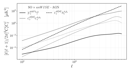
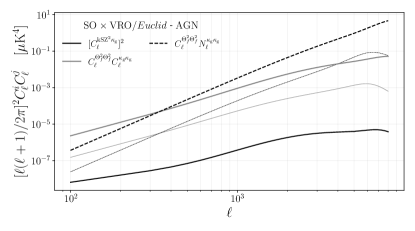
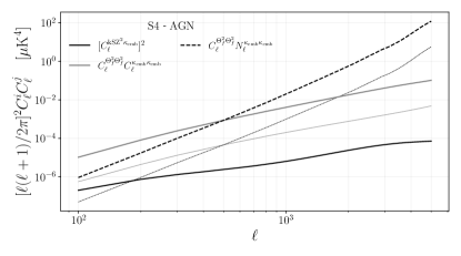
In the right panels of Figure 10, we show the different contributions to the covariance matrix for the three types of cross-correlations. In all cases, the high-$\ell$ regime is dominated by noise from the LSS tracer. This suggests that future surveys, beyond the ones considered here, will improve the sensitivity.

3.6 CMB Lensing Contribution

The procedure to measure the projected-field kSZ power spectrum relies on squaring the CMB temperature map. Inevitably, this implies that the measurement picks up correlations from the lensing field whose leading-order contribution is of the form $\langle\psi X\rangle\langle\Theta_{u}\Theta_{u}\rangle$ where $\Theta_{u}$ is the unlensed CMB temperature field and $\psi$ is the CMB lensing potential. This simply arises from the fact that the lensed CMB temperature field is $\Theta=\Theta_{u}+\nabla\psi\cdot\nabla\Theta_{u}+\cdots$. Hence, the leading-order lensing contribution to $\bar{C}_{\ell}^{\mathrm{kSZ}^{2}X}$ is (see Ferraro et al., 2016, for details):

$$C_{\ell}^{\Theta_{u}^{2}\psi X}=-2\ell\frac{C_{\ell}^{\psi X}}{(2\pi)^{2}}\int\mathrm{d}\bm{\ell}^{\prime}\ell^{\prime}w(\ell^{\prime})C_{\ell^{\prime}}^{\Theta_{u}\Theta_{u}}w(|\bm{\ell}^{\prime}+\bm{\ell}|)\cos\theta,$$ (60)

where $\theta=\hat{(\bm{\ell},\bm{\ell}^{\prime})}$, $C_{\ell}^{\Theta_{u}\Theta_{u}}$ is the unlensed primary CMB power spectrum, and $C_{\ell}^{\psi X}$ is the cross-power spectrum between the lensing potential and tracer $X$, which we write in terms of the CMB lensing convergence as $C_{\ell}^{\psi X}=[{2}/{\ell(\ell+1)}]C_{\ell}^{X\kappa_{{}_{\mathrm{CMB}}}}$. We compute $C_{\ell}^{X\kappa_{{}_{\mathrm{CMB}}}}$ within the halo model (see Appendix B.9.4). Note also that since the cosine can be expanded as $\cos\theta=(|\bm{\ell}^{\prime}+\bm{\ell}|^{2}-\ell^{2}-\ell^{\prime 2})/2\ell\ell^{\prime}$, we can compute Eq. (60) efficiently with FFT methods.

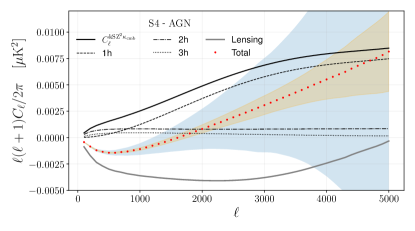
The lensing contribution is shown as the thick grey line in the left panels of Figure 10. At low-$\ell$ this contribution is negative and generally larger than the kSZ term. At larger $\ell$ the lensing contribution remains smaller than the kSZ contribution for all the cases shown here. In the Planck-based analyses of Hill et al. (2016) and Kusiak et al. (2021) the lensing contribution dominated over most of the $\ell$-range. The difference is that here we are showing predictions for SO and CMB-S4 CMB maps, which probe scales beyond $\ell\sim 3000$ where the kSZ effect dominates the anisotropy (see Figure 1), unlike Planck, for which the lensed CMB dominates over the kSZ signal on the relevant scales.

Figure 10: Contributions to the projected-field kSZ power spectrum measurements (left column) and covariance matrix (right column) in cross-correlation with galaxy number density (top, assuming unWISE), galaxy weak lensing (middle, assuming a VRO/Euclid-like survey), and CMB weak lensing (bottom, assuming CMB-S4 CMB lensing). For the CMB map specifications see Table 1, and for the LSS survey specifications see Table 3. In the left plots, the lensing contribution of Eq. (60) is the thick grey line; the shaded areas show the statistical uncertainty computed with the covariance matrix of Eq. (58). In the right panels, the thin lines show the contributions without the CMB temperature map noise. In the left panels, the orange area indicates the size of the error bars assuming no CMB temperature map noise, i.e., the cosmic-variance-limited CMB measurement. The CMB noise levels are shown in Figure 1. Note that for this spectra we used a linear binning with $\Delta\ell=100$.

Experiment	Tracer	Specifications
unWISE	$\delta_{\mathrm{g}}$	$f_{\mathrm{sky}}=0.6$; blue HOD from Kusiak et al. (2022); $N_{\ell}^{\delta_{\mathrm{g}}\delta_{\mathrm{g}}}=8.94\times 10^{-8}$ ($\bar{n}=3409\,\mathrm{deg}^{-2}$)
DES-like	$\kappa_{\mathrm{g}}$	$f_{\mathrm{sky}}=0.12$; $n_{s}=8\,\mathrm{arcmin}^{-2}$, $\sigma_{\gamma}^{2}=0.3$; $n(z)$= sources bin 3 (Zacharegkas et al., 2021)
VRO/Euclid-like	$\kappa_{\mathrm{g}}$	$f_{\mathrm{sky}}=f_{\mathrm{sky}}^{{}_{\mathrm{CMB}}}$; $n_{s}=40\,\mathrm{arcmin}^{-2}$, $\sigma_{\gamma}^{2}=0.3$; $n(z)$= sources bin 3 (Zacharegkas et al., 2021)
SO CMB Lensing	$\kappa_{\mathrm{cmb}}$	truncation at $\ell_{\mathrm{max}}=5000$; noise curve from online repository (see footnote 15).
CMB-S4 CMB Lensing	$\kappa_{\mathrm{cmb}}$	truncation at $\ell_{\mathrm{max}}=5000$; noise curve from online repository (see footnote 16).

Table 3: Specifications for the LSS survey experiments considered in our forecast analysis. For VRO/Euclid, $f_{\mathrm{sky}}=f_{\mathrm{sky}}^{{}_{\mathrm{CMB}}}$ assumes that the sky area is limited by the sky coverage and mask of the CMB map (see Table 1 for the $f_{\mathrm{sky}}^{{}_{\mathrm{CMB}}}$ values).

Figure 11: Projected-field kSZ power spectrum in cross-correlation with galaxy number density (top, assuming unWISE), galaxy weak lensing (middle, assuming a DES-like and a VRO/Euclid-like survey), and CMB weak lensing (bottom, assuming SO and CMB-S4). For the CMB map specifications see Table 1 and for the LSS survey specifications see Table 3. Each color corresponds to a different gas profile assumption: NFW, Adiabatic, or AGN Feedback (see Table 2 and Eq. 44). The shaded areas (or error bars) represent the statistical uncertainty computed with the covariance matrix of Eq. (58). The spectra in this figure are computed with a bin size of $\Delta\ell=264$.

4 Forecasts

In this section we forecast the detection signal-to-noise for the projected-field kSZ power spectrum signal and for some of the gas profile parameters, including its normalization (determined by $f_{\mathrm{b}}f_{\mathrm{free}}$), the inner slope $\alpha$, and the outer slope $\beta$ (see Subsection 3.2). Our forecasts are obtained with the Fisher matrix formalism (e.g., Tegmark et al., 1997). The results depend on the characteristics of the CMB and LSS tracer maps which enter the covariance matrix calculation (resolution, noise, sky coverage and overlap, etc). We consider four CMB maps:

• Planck (Planck Collaboration et al., 2018), as in Hill et al. (2016) and Kusiak et al. (2021). In our fiducial calculations we compute the noise with $\Delta_{T}=47\,\mu\mathrm{K}$-arcmin, matching that in the LGMCA CMB map Bobin et al. (2016), and use $f_{\mathrm{sky}}=0.6$. For the beam we use $\Theta_{\mathrm{FWHM}}=5$ arcmin. In the Wiener filter we set $\ell_{\mathrm{max}}=3000$.

• AdvACT (Henderson et al., 2016) for upcoming maps from ACT (e.g., Aiola et al., 2020). We use $\Delta_{T}=20\,\mu\mathrm{K}$-arcmin and $f_{\mathrm{sky}}=0.3$ for the noise and covariance matrix, with $\Theta_{\mathrm{FWHM}}=1.5$ arcmin and $\ell_{\mathrm{max}}=8000$ for the beam and Wiener filter. The noise level here has been inflated over the raw temperature map noise in order to account for the effects of component separation, using the same ILC methodology as applied in the SO and CMB-S4 calculations below.

• Simons Observatory (SO; Ade et al., 2019), for next-generation CMB maps. We use $f_{\mathrm{sky}}=0.4$ in the covariance matrix, with $\Theta_{\mathrm{FWHM}}=1.4$ arcmin and $\ell_{\mathrm{max}}=8000$ for the beam and Wiener filter. For the noise, we use the post-ILC component-separated noise curves constructed in Ade et al. (2019) (see Sec. 2.4-2.5 of that work), which are available online. These noise curves are constructed using a harmonic ILC method applied to simulated sky maps containing all relevant Galactic and extragalactic foregrounds. For simplicity, we use the standard minimum-variance ILC noise curves here, although in an actual analysis it may be necessary to apply constrained ILC methods to deproject contamination arising from the thermal SZ effect or the cosmic infrared background.

• CMB-Stage 4 (CMB-S4; Abazajian et al., 2019), with the same assumptions as SO, but different post-ILC component-separated noise curves. The CMB-S4 noise curves are also publicly available online and were computed with the same methodology as the SO post-ILC noise curves (see Appendix A.3 of Abazajian et al. (2019)).

These specifications are summarized in Table 1 and the CMB temperature map noise curves are shown in Figure 1. For the LSS survey data, we consider five configurations for different tracers:

• unWISE (Schlafly et al., 2019) galaxy number density, i.e., $X=\delta_{\mathrm{g}}$, as in Krolewski et al. (2020); Kusiak et al. (2021). For halo-model calculations, we characterize the galaxy-halo connection using the HOD results for the blue sample obtained in Kusiak et al. (2022). See Appendix B.8 for details on the HOD parameters. For the shot noise we set $N_{\ell}^{\delta_{\mathrm{g}}\delta_{\mathrm{g}}}=8.94\times 10^{-8}$, which corresponds to $1/\bar{n}$ with $\bar{n}=3409\,\mathrm{deg}^{-2}$ (from Krolewski et al., 2020) converted to steradians.

• DES-like galaxy weak lensing, i.e., $X=\kappa_{\mathrm{g}}$, assuming a galaxy weak lensing survey similar to DES-Y3 (e.g., Sevilla-Noarbe et al., 2021), with $f_{\mathrm{sky}}=0.12$ (i.e., 5000 deg² sky area) a source galaxy number density $n_{s}=8\,\mathrm{arcmin}^{-2}$ and shape noise $\sigma_{\gamma}^{2}=0.3$. For the source galaxy redshift distribution, we take the distribution of the third redshift bin of the Redmagic sample peaking at $z\approx 0.7$ (the dashed red line in the top panel of Figure 3 of Zacharegkas et al., 2021).

• VRO/Euclid-like galaxy weak lensing, i.e., $X=\kappa_{\mathrm{g}}$, assuming a galaxy weak lensing survey similar to VRO (Chisari et al., 2019) or Euclid (Blanchard et al., 2020), with the same source distribution and shape noise as above, but a galaxy source density five times larger, $n_{s}=40\,\mathrm{arcmin}^{-2}$, and full overlap with the CMB maps.

• SO CMB lensing, i.e., $X=\kappa_{\mathrm{cmb}}$, with the reconstructed CMB lensing noise curve from the online repository, which is built by applying the lensing quadratic estimator to the same post-ILC noise curves described above. Note that we truncate the power spectra at $\ell_{\mathrm{max}}=5000$ (since there is no SNR beyond this multipole).

• CMB-S4 CMB lensing, i.e., $X=\kappa_{\mathrm{cmb}}$, with the reconstructed CMB lensing noise curve from the online repository and truncating at $\ell_{\mathrm{max}}=5000$.

These specifications are summarized in Table 3 and the SO and CMB-S4 CMB lensing noise curves are shown in Figure 19 of the Appendix.

The Fisher matrix is computed using the analytical covariance matrix (see Subsection 3.5) and the halo model predictions for the projected-field kSZ power spectrum (see Subsection 3.2). With the lensing contribution included (see Subsection 3.6), the total signal is $\bar{C}_{\ell}^{\mathrm{kSZ}^{2}X}=C_{\ell}^{\mathrm{kSZ}^{2}X}+C_{\ell}^{\Theta_{u}^{2}\psi X}$. (Note the over-bar to distinguish the total signal from the kSZ signal only.) Then the Fisher matrix elements are

$$F_{ij}=\sum_{aa^{\prime}}\frac{\partial\bar{C}_{a}^{\mathrm{kSZ}^{2}X}}{\partial p_{i}}[M^{-1}]_{a{a^{\prime}}}\frac{\partial\bar{C}_{a^{\prime}}^{\mathrm{kSZ}^{2}X}}{\partial p_{j}}$$ (61)

where $p$ denotes the vector of varied parameters, $i,j$ are the varied parameter indices, and $a$ is the multipole bin index. With this, the marginalized 1$\sigma$ uncertainty on a parameter $p_{i}$ is given by $\sqrt{[F^{-1}]_{ii}}$. The binning of the covariance matrix is discussed in Subsection 3.5. For the binned power spectrum we simply assume that is it well approximated by the value at the center of the bin. Note that we use a linear binning with $\Delta\ell=564$ and $\ell_{\mathrm{min}}=100$ for the Fisher forecasts.

To start, we compute the total detection signal-to-noise ratio, SNR_tot. We can define a single parameter, $A_{\mathrm{kSZ^{2}}}$, such that $C_{\ell}^{\mathrm{kSZ}^{2}X}=A_{\mathrm{kSZ^{2}}}C_{\ell}^{\mathrm{kSZ}^{2}X,fid.}$ where $C_{\ell}^{\mathrm{kSZ}^{2}X,fid.}$ is the fiducial prediction, corresponding to $A_{\mathrm{kSZ^{2}}}=1$. In this case, the derivatives in Eq. (61) are straightforward and the Fisher calculation yields

$$\mathrm{SNR}_{\mathrm{tot}}=\left(\frac{\Delta{A}_{\mathrm{kSZ^{2}}}}{{A}_{\mathrm{kSZ^{2}}}}\right)^{-1}=\sqrt{F}=\left[\sum_{a}\frac{(C_{a}^{\mathrm{kSZ}^{2}X,fid.})^{2}}{M_{aa}}\right]^{1/2}.$$ (62)

Results are reported in the first column of Table 4. The highest SNR values are obtained for galaxy number density cross-correlation. For Planck $\times$ unWISE we find $\mathrm{SNR}_{\mathrm{tot}}=1.7$, consistent with the measurement in Kusiak et al. (2021), which reported $\mathrm{SNR}_{\mathrm{tot}}=1.35$ (for the unWISE blue galaxy sample). With data that is already on hand, e.g., AdvACT CMB maps and unWISE galaxies, we forecast a detection SNR over 10$\sigma$. In the next decade, with CMB-S4 $\times$ unWISE, the SNR should reach $\gtrsim 100\sigma$. For galaxy-density cross-correlation, we note that $A_{\mathrm{kSZ^{2}}}$ is degenerate with the galaxy bias, $b_{\mathrm{g}}$ (which also determines the amplitude of the lensing term). Nonetheless, the galaxy bias can be tightly constrained by galaxy clustering ($C_{\ell}^{\delta_{\mathrm{g}}\delta_{\mathrm{g}}}$) and galaxy-lensing cross-correlation ($C_{\ell}^{\delta_{\mathrm{g}}\kappa_{\mathrm{g}}}$) measurements. If we set a Gaussian prior on $b_{\mathrm{g}}$ corresponding to the measurements of Krolewski et al. (2020), we find that the $\mathrm{SNR}_{\mathrm{tot}}$ forecasts only change marginally.

Galaxy weak lensing cross-correlation based on DES data ($\mathrm{SNR_{tot}}\approx 10$ with CMB-S4) do not reach SNR values as high as with galaxy density (due to the influence of shape noise), but with VRO/Euclid we expect clear detections of this cross-correlation as well ($\mathrm{SNR_{tot}}\approx 30$ with CMB-S4). A detection with CMB lensing cross-correlation will certainly require next-generation CMB maps such as those from SO and CMB-S4, for which we find $\mathrm{SNR_{tot}}\approx 16$ and $\mathrm{SNR_{tot}}\approx 35$, respectively.

With such high SNR detections, we can ask how well different gas profile shapes could be distinguished. In Figure 11 we see that galaxy density cross-correlation using unWISE will be able to exclude particular gas profile models at high significance. It appears to be more challenging with galaxy weak lensing or CMB lensing cross-correlations, but forecasts with SO $\times$ VRO/Euclid (galaxy weak lensing) and CMB-S4 (CMB weak lensing) are promising.

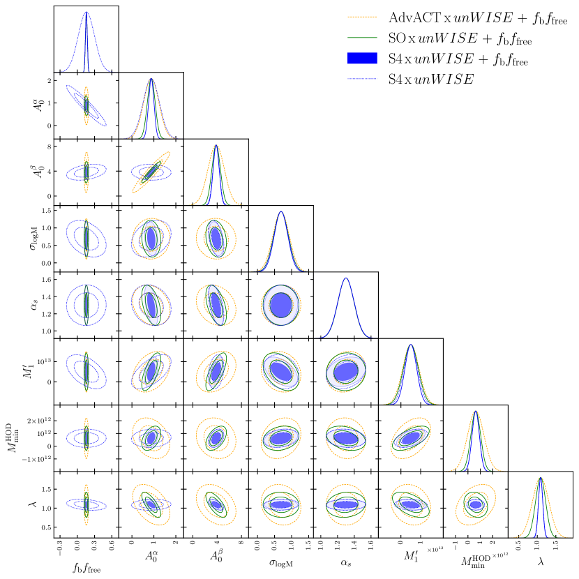
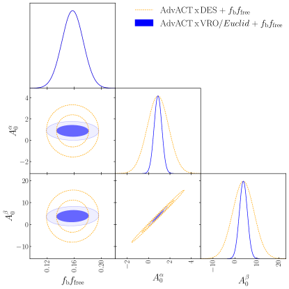
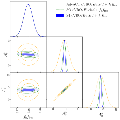
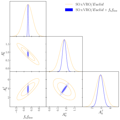
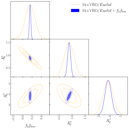
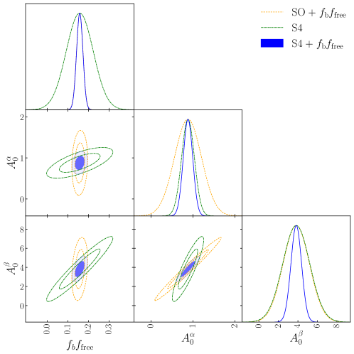
A more refined way to answer this question is to study forecasts on the gas profile parameters. There are three parameters: first, the overall amplitude of the gas density profile (i.e., the parameter $C$ in Eq. 44 which is completely degenerate with the product of the free electron and baryon fractions, $f_{\mathrm{b}}f_{\mathrm{free}}$; second, the parameter $\alpha$ controlling the inner slope of the profile; third, the parameter $\beta$ controlling the outer slope of the profile. We compute the Fisher matrix for these gas profile parameters. To do so, we evaluate the derivatives in Eq. (61) around the fiducial model. The Fisher confidence ellipses are shown in Figure 12 for cross-correlation with galaxy number density, in Figure 13 for galaxy weak lensing, and in Figure 14 for CMB weak lensing. The marginalized constraints are reported in Table 4. Since the baryon fraction at large halo-centric radii should be close to the cosmological value $\Omega_{\mathrm{b}}/\Omega_{\mathrm{m}}$ and the free electron fraction close to unity because the universe is fully reionized at low redshift, we can safely assume an external constraint on $f_{\mathrm{b}}f_{\mathrm{free}}$. In Table 4 the forecasts where we have imposed a 10% prior on $f_{\mathrm{b}}f_{\mathrm{free}}$ are reported in parentheses.

		SNRtot	$(\frac{\Delta A_{0}^{\mathrm{\beta}}}{A_{0}^{\mathrm{\beta}}})^{-1}$	$(\frac{\Delta A_{0}^{\mathrm{\alpha}}}{A_{0}^{\mathrm{\alpha}}})^{-1}$	$(\frac{\Delta f_{\mathrm{free}}}{f_{\mathrm{free}}})^{-1}$
{45mm[$\delta_{\mathrm{g}}$]	Planck $\times$ unWISE	1.7	0.18 (0.37)	0.29 (0.38)	0.19 (10)
	AdvACT $\times$ unWISE	17.8	1.72 (2.87)	2.22 (2.54)	0.71 (10)
	SO $\times$ unWISE	61.9	3.70 (5.51)	2.07 (4.98)	0.78 (10)
	CMB-S4 $\times$ unWISE	102.9	7.32 (7.83)	2.38 (7.18)	1.12 (10)
{65mm[$\kappa_{\mathrm{g}}$]	AdvACT $\times$ DES	2.24	0.28 (0.79)	0.59 (0.88)	0.09 (10)
	AdvACT $\times$ VRO/Euclid	5.98	0.92 (2.11)	1.72 (2.44)	0.31 (10)
	SO $\times$ DES	6.14	1.03 (2.75)	0.93 (2.34)	0.23 (10)
	SO $\times$ VRO/Euclid	18.81	3.89 (6.84)	3.24 (8.22)	0.88 (10)
	CMB-S4 $\times$ DES	9.71	2.19 (4.36)	1.33 (5.23)	0.40 (10)
	CMB-S4 $\times$ VRO/Euclid	29.72	8.57 (13.07)	4.71 (15.08)	1.51 (10)
{28mm[$\kappa_{\mathrm{cmb}}$]	SO	16.39	0.92 (2.84)	1.72 (2.72)	0.94 (10)
	CMB-S4	34.52	2.76 (7.01)	5.75 (7.79)	2.4 (10)

Table 4: Forecasts for projected-field kSZ power spectrum detection significance (first column), gNFW parameters for the gas profile (second and third column), and the free electron fraction (last column). Numbers quoted in parentheses are computed assuming a 10% prior on $f_{\mathrm{free}}$. Note that we assume our fiducial AGN feedback model in all calculations here (see Table 2). Note that $\delta_{g}$ forecasts have been marginalized over HOD parameters, while this is not necessary for the lensing cross-correlation forecasts (since they do not depend on galaxy HOD’s).

For cross-correlation with galaxy density, we also take into account the uncertainties on the HOD parameters (see Appendix  B.8) by using priors corresponding to the marginalized 1$\sigma$ uncertainty found in Kusiak et al. (2022). In this case, the peculiar scale dependence of the lensing contribution, which depends on HOD parameters, also helps to break degeneracies with the gas profile parameters (see Figure 12 for the contour plots including HOD parameters).

For all the cross-corelations (galaxy density, galaxy lensing, and CMB lensing) we see that $\alpha$ and $\beta$ are always degenerate. This is because a larger $\alpha$ can be compensated by a larger $\beta$, consistent with the results of Figure 9, which shows that these parameters mainly change the amplitude of the projected field power spectrum in a rather scale-independent manner. That means that the slope parameters are also strongly degenerate with $f_{\mathrm{b}}f_{\mathrm{free}}$ (see dotted blue contours in Figure 12, dotted orange contours in Figure 13, and dotted green contours in Figure 14). These degeneracies can be significantly reduced with a prior on $f_{\mathrm{b}}f_{\mathrm{free}}$. Still, it is worth noting that even without external information on $f_{\mathrm{b}}f_{\mathrm{free}}$, CMB-S4 CMB maps should allow high significance measurements of $\alpha$ and $\beta$. Indeed, for CMB-S4 $\times$ unWISE (galaxy density cross-correlation) we forecast a 7$\sigma$ measurement of $\beta$. For CMB-S4 $\times$ VRO/Euclid (galaxy weak lensing cross-correlation) we forecast a 9$\sigma$ measurement of $\beta$ and a 5$\sigma$ measurement of $\alpha$. And for the CMB-S4 kSZ²–CMB lensing cross-correlation we find that, unlike galaxy density or galaxy lensing cross-correlation, the inner slope is better measured ($6\sigma$) than the outer slope ($3\sigma$).

As can be seen in Figure 12, and in the bottom plots of Figure 13, the addition of an external prior on $f_{\mathrm{b}}f_{\mathrm{free}}$ allows us to constrain the slope parameters with forthcoming SO CMB maps before CMB-S4 will become available. For SO $\times$ unWISE (galaxy density cross-correlation) we forecast 5$\sigma$ measurements of both $\alpha$ and $\beta$. With SO $\times$ VRO/Euclid (galaxy weak lensing cross-correlation) we find 7$\sigma$ for $\beta$ and 8$\sigma$ for $\alpha$. With CMB-S4 maps and the prior on $f_{\mathrm{b}}f_{\mathrm{free}}$ the significance of the forecasted measurements of $\alpha$ and $\beta$ is roughly two times larger than without the external prior.

With readily available AdvACT CMB maps, although we forecast high SNR detections of the projected-field power spectrum, a measurement of the slope parameters appears to be more challenging owing to the degeneracies discussed above. With the external prior on $f_{\mathrm{b}}f_{\mathrm{free}}$, we forecast measurements of $\alpha$ and $\beta$ at a significance of $\sim 2\sigma$ in cross-correlation with unWISE galaxies and VRO/Euclid weak lensing data. Nonetheless, we emphasize that our forecasts are conservative in the sense that they rely on the AGN feedback gas density model, which yields a low projected-field power spectrum compared to the NFW and Adiabatic models (see Figure 5, 6, 7, and 11 for comparisons of the respective predictions). It is possible that the spatial distribution of the gas around real halos is significantly different than the AGN feedback model and could be measured with the the projected-field power spectrum using AdvACT or SPT CMB maps.

Figure 12: 2D marginalized posterior probability distribution from Fisher matrix calculations for kSZ²-galaxy density cross-correlation. Galaxies are assumed to be the unWISE blue sample. The orange and green lines assume AdvACT and SO CMB maps, respectively, as well as a 10% prior on $f_{\mathrm{free}}$. The blue contours are with CMB-S4 CMB maps with (filled) and without (empty) the prior on $f_{\mathrm{b}}f_{\mathrm{free}}$.

Figure 13: 2D marginalized posterior probability distributions from Fisher matrix calculations for kSZ²-galaxy weak lensing cross-correlation. (Top Left:) AdvACT CMB maps with DES (orange) and VRO/Euclid (blue) galaxy weak lensing, with a 10$\%$ prior on $f_{\mathrm{free}}$ in both cases. (Top right:) AdvACT (orange), SO (green), and CMB-S4 (blue) CMB maps with VRO/Euclid galaxy weak lensing, with a 10$\%$ prior on $f_{\mathrm{b}}f_{\mathrm{free}}$ in all cases. (Bottom Left:) SO CMB maps with VRO/Euclid galaxy weak lensing, with (blue) and without (orange) a 10$\%$ prior on $f_{\mathrm{free}}$. (Bottom Right:) Same as bottom left but with CMB-S4 CMB maps.

Figure 14: 2D marginalized posterior probability distribution from Fisher matrix calculations for kSZ²-CMB lensing cross-correlation. The orange line assumes SO CMB maps and a 10% prior on $f_{\mathrm{b}}f_{\mathrm{free}}$. The blue and green lines assume CMB-S4 CMB maps with and without a 10% prior on $f_{\mathrm{b}}f_{\mathrm{free}}$, respectively.

5 Conclusion

Our main results are the first calculation of the projected-field kSZ power spectrum using the halo model formalism and its numerical implementation in class_sz (Section 3) for galaxy density, galaxy weak lensing, and CMB weak lensing cross-correlations. Improving upon previous works by Doré et al. (2004), DeDeo et al. (2005), and Ferraro et al. (2016) that were based on an effective approach for the computation of the hybrid bispectrum (Subsection 2.4), the halo model formalism allows us to access the scale-dependent information on the gas distribution around halos. Since the projected-field power spectrum is an integral of a three-point function (i.e., the hybrid bispectrum), the halo model expressions are a sum of a 1-halo, 2-halo, and 3-halo term. We find that the 1-halo term largely dominates for $\ell\gtrsim 500$ (see Figure 5, 6, and 7).

An important aspect of the numerical implementation is to take advantage of the separable form of the expressions so we can evaluate integrals as products in Fourier space, using FFTLog methods for the Fourier transforms (Subsection 3.4). This speeds up the computation by a factor of $\sim 100$ compared to trapezoidal or quadrature rules. Still, the evaluation of a projected-field power spectrum takes $\mathcal{O}(10\mathrm{s})$ on a laptop. This may be too time-consuming for a fast Monte-Carlo-Markov-Chain parameter inference analysis. In order to accelerate MCMCs, it will be profitable to develop emulators using existing codes such as cosmopower (Mancini et al., 2022).

Projected-field power spectrum measurements require Wiener filtering of the CMB temperature map in order to mitigate foreground contamination and maximize the detection significance (Subsection 2.3). As a secondary improvement, we found a Wiener filter that is more optimal than the previous ansatz and justified it with a heuristic derivation (Appendix C.1). We leave for future work the task of finding a rigorous derivation of the optimal filter.

We parameterized the gas density profile using a gNFW formula with parameters calibrated on hydrodynamical simulations from Battaglia (2016). We computed halo model predictions for three different shapes of the gas profile, motivated by different physical assumptions on feedback mechanisms, namely an NFW-like model, an Adiabatic model, and an AGN feedback model (Subsection 3.3). Regarding the subtle treatment of the truncation of the gas density profile, necessary to obtained a converged Fourier transform, we proposed a procedure that preserves the total gas mass without altering the scale dependence of the profile (see text around Eq. 47). For a fixed total gas mass, the gas profile extends toward larger radius in the Adiabatic model compared to the NFW model and even more so in the AGN feedback model (Figure 4), in accordance with the fact that energetic mechanisms tend to push the gas from the center towards outer regions of halos. Because of this, the projected-field power spectrum is the lowest in the AGN feedback model. Although we focused on the Battaglia (2016) parameterization, the formalism presented here can be easily extended to other gas density profiles. For instance, motivated by recent results from simulations (Lee et al., 2022) and observations (Pandey et al., 2021), it will be interesting to include a more general dependence on halo concentration and allow for a broken power law mass dependence of the gas density profile. As cosmological inference is moving into a stage where it relies heavily on non-analytical models trained on results from simulations, it will also be beneficial to extend our numerical implementation so that it can accomodate emulators for the gas density profiles (e.g., Moser et al., 2022) and the halo mass function (e.g., Bocquet et al., 2020).

We found that the halo model predictions roughly match the previous effective approach predictions for galaxy density cross-correlation (Figure 5). However, they are significantly lower for weak lensing cross-correlation (Figure 6 and 7).

The low-$\ell$ behavior of the projected-field power spectrum when we change the gas density profile shape is not straightforward to interpret. The naive expectation that the low-$\ell$ limit should be independent of the scale dependence of the gas density profile because it is determined by the total gas mass does not hold here. In fact, the low-$\ell$ limit also receives contributions from small scales probing the inner part of halos. This is because of the convolution in harmonic space that arises from the real-space squaring operation of the CMB temperature field. We found that variations of the inner and outer slopes of the profiles mainly amount to a scale-independent rescaling of the projected field power spectrum at the sensitivity level of near-term data (Figure 9), although there is a noticeable scale-dependent effect associated with the outer slope for CMB weak lensing cross-correlation.

We also used the halo model to estimate the covariance matrix of the projected-field power spectrum (Subsection 3.5) and the CMB lensing contribution to the measured signal (Subsection 3.6).

We assumed that the covariance matrix is dominated by the Gaussian contribution and neglected contributions from higher-point functions, i.e., in this case a connected 6-point function, combinations of 3-point functions, and combinations of 4- and 2-point functions. As an example, we neglect terms like a $\langle TTTT\rangle\langle XX\rangle$ term, i.e., the connected 4-pt function of $T$ generated by lensing and the trispectrum of the foregrounds and kSZ, which are expected to be small. At some point these higher order terms should be investigated, but the Gaussian contributions certainly dominate for the forecasts considered here (see, e.g., Coulton et al., 2020, for an analysis of non-Gaussian covariance for the primordial bispectrum from CMB observations).

For the covariance matrices we considered four classes of CMB maps (Planck, AdvACT, SO, and CMB-S4) characterized by different resolutions and noise properties (Table 1) in combination with five LSS survey configurations, namely: unWISE for galaxy density, DES and VRO/Euclid for galaxy weak lensing, and SO and CMB-S4 for CMB weak lensing (Table 3).

With these experimental specifications we obtained Fisher forecasts on the total detection SNR of the projected-field power spectrum and on measurements of the inner slope $\alpha$ and outer slope $\beta$ of the gas density profile (Table 4 in Section 4), accounting for degeneracies with HOD parameters present in galaxy density cross-correlation (Figure 12). We found that galaxy density cross-correlation will be the easiest to detect with current datasets ($\mathrm{SNR}_{\mathrm{tot}}=17.8$ with AdvACT $\times$ unWISE) although it will be challenging to probe the radial shape of the profiles. A first measurement of the slopes of the density profile, using galaxy density cross-correlation should be achievable with SO CMB maps. For galaxy weak lensing cross-correlation, we forecast a first robust detection (above $5\sigma$) with AdvACT $\times$ VRO/Euclid and high-significance measurements of the profile slopes with SO CMB maps. CMB lensing cross-correlation detections should be possible with SO CMB maps and measurements of the slopes with CMB-S4 maps. Interestingly, CMB lensing cross-correlation seems to be more sensitive to the inner slope of the profile than the outer slope, while galaxy density and galaxy lensing cross-correlations appear to probe both parameters equally well. Whether this is an artefact of our approximations or a real feature will be assessed in future work.

Although current SNR forecasts are often higher for cross-correlation with galaxy number density, studying cross-correlations with CMB or galaxy weak lensing is a particularly appealing avenue because it is free of degeneracies with HOD parameters or galaxy bias. Moreover, cross-correlation with CMB lensing can yield a measurement of the gas profile from all halos up to $z\approx 2-3$ (without selection effects), while cross-correlation with galaxy weak lensing should enable gas tomography depending on the redshift distribution of the source galaxies.

We note that the halo model formalism we presented here can be extended to other cross-correlations. For instance, kSZ²-21cm cross-correlation has been shown to open a unique window on patchy reionization (see, e.g., Ma et al., 2018; La Plante et al., 2020; La Plante et al., 2022). Our formalism can also be used to compute the full three-point function (the hybrid bispectrum) which should carry more information than the projected-field power spectrum.

A priority for future work will be to establish the robustness of the modeling choices based on further analytical investigations (e.g., Patki & Battaglia, 2022) and comparison with hydrodynamical simulations, building on the initial comparisons in Hill et al. (2016) and Ferraro et al. (2016). State-of-the-art simulations that could be used for such investigations include cosmological hydrodynamical simulations like Illustris TNG (Springel et al., 2017; Nelson et al., 2018) and BAHAMAS (McCarthy et al., 2016), or baryon pasting simulations such as the ones presented in Osato & Nagai (2022).

This work continues to pave the way for kinetic SZ measurements with upcoming CMB observations and LSS surveys to become a major source of information on the ICM and CGM gas thermodynamics (e.g., Battaglia et al., 2019). This is an increasingly important research topic, as current cosmological analyses show signs of inconsistencies which could be due to our misunderstanding of the behavior of baryonic matter in dense regions of the universe (e.g., Amon & Efstathiou, 2022). Understanding baryons will be crucial in order to maximize cosmological information extraction from ongoing and upcoming LSS surveys.

Data Availability

The code class_sz is public. All numerical computations presented in this paper are reproducible using a Jupyter notebook online. We used getdist (Lewis, 2019) for computing the Fisher contours.

Appendix A Velocity dispersion

In Figure 15 we show the velocity dispersion, as computed in Eq. (22) with different choices for the matter power spectrum. In our fiducial model (as in, e.g., Kusiak et al., 2021), we use the non-linear matter power spectrum computed with halofit (dotted line). With this, we get $\sigma_{v}^{2}\simeq 1.55\times 10^{-6}$ of $v_{\mathrm{rms}}^{2}\simeq 648\,\mathrm{km/s}$. The computation with the hmcode non-linear matter power spectrum is nearly identical to the halofit one. If we use the linear matter power spectrum instead (as in, e.g., Ferraro et al., 2016; Hill et al., 2016), the velocity dispersion is $\approx 30\%$ lower at $z=0$ – we get $\sigma_{v}^{2}\simeq 1.05\times 10^{-6}$ of $v_{\mathrm{rms}}^{2}\simeq 531\,\mathrm{km/s}$. This difference would propagate linearly into the projected-field kSZ power spectrum, since it is proportional to $\sigma_{v}^{2}$ (in our approximation, see Eq. 32).

Figure 15: Velocity dispersion (Eq. 22) with different matter power spectrum choices, computed with class_sz. We assumed our fiducial cosmology.

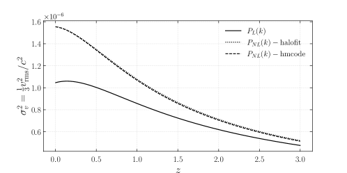
Appendix B Useful Halo Model Tools

The halo model (Scherrer & Bertschinger, 1991; Mo & White, 1996; Seljak, 2000; Scoccimarro et al., 2001; Ma & Fry, 2000; Peacock & Smith, 2000; Cooray & Sheth, 2002) is an analytic model to compute power spectra, bispectra and higher order statistics of LSS tracers.

B.1 Halo Mass Function

The model assumes that matter is distributed within distinct spherical halos whose abundance is determined by the linear matter power spectrum through the halo mass function (HMF). The HMF determines the comoving number density of haloes of mass $M$ at redshift $z$ via (e.g, Press & Schechter, 1974; Bond et al., 1991; Tinker et al., 2008, 2010)

$$\frac{\mathrm{d}n}{\mathrm{d}m}=\nu f(\nu)\frac{\rho_{\mathrm{m,0}}}{m}\frac{\mathrm{d}\ln\sigma^{-1}}{\mathrm{d}m}$$ (B1)

where $\nu=\delta_{c}/\sigma$ is the peak height in the linear density field with $\delta_{c}=(3/20)(12\pi)^{2/3}\approx 1.686$ the spherical collapse density threshold (see Nakamura & Suto, 1997, for the $\Omega_{\mathrm{m}}$ correction - not used here), $\rho_{\mathrm{m,0}}$ is the mean matter density at $z=0$ and

$$\sigma^{2}(m,z)=\frac{1}{2\pi^{2}}\int\mathrm{d}kk^{2}\hat{\mathrm{W}}(kR)^{2}P_{L}(k,z)$$ (B2)

is the variance of the matter density field smoothed in region of radius $R=(3m/4\pi\rho_{\mathrm{m,0}})^{1/3}$ using the Fourier transform of the real-space top-hat window function $\hat{\mathrm{W}}(x)=3j_{1}(x)/x$ where $j_{1}(x)=\left[\sin(x)-x\cos(x)\right]/x^{2}$ is the first-order spherical Bessel function. Here, $P_{L}$ is the linear matter power spectrum. In this paper, we use the Tinker et al. (2008) formula (see their Eq. 3) for the function $f(\nu)$ rather than the Tinker et al. (2010) formula for the same reasons as explained in Appendix B of Kusiak et al. (2022). One should keep in mind that these fitting formulas are calibrated on simulations with a limited mass and redshift range. Namely $0.25\lesssim\sigma^{-1}\lesssim 2.5$, which corresponds to masses $\sim 10^{10}-10^{15}\,\mathrm{M}_{\odot}/h$ at $z=0$) and $0<z\lesssim 2$. Tinker et al. (2008) suggests to use $f(\sigma,z=2.5)$ for all $z>2.5$, while Tinker et al. (2010) suggests to use $f(\sigma,z=3)$ for all $z>3$.

By consistency, the HMF must be such that

$$\int\mathrm{d}\nu f(\nu)=1,\quad\int\mathrm{d}\nu b^{(1)}(\nu)f(\nu)=1,\quad\int\mathrm{d}\nu b^{(n)}(\nu)f(\nu)=0\,\,\mathrm{for}\,\,n>1,$$ (B3)

where $b^{(1)}$ is the linear bias (see Eq. B13) and $b^{(n)}$ are are higher order biases. These constraints enforce that all matter is within halos and that it is not bias with respect to itself (e.g., Tinker et al., 2010).

B.2 Consistency Conditions

To impose the consistency conditions numerically, the mass integrals are approximated as follows (Schmidt, 2016):

$$\int_{0}^{+\infty}\mathrm{d}n\hat{u}^{X}(m,z)\hat{u}^{Y}(m,z) =\int_{m_{\mathrm{min}}}^{m_{\mathrm{max}}}\mathrm{d}n\hat{u}^{X}(m,z)\hat{u}^{Y}(m,z)+N_{\mathrm{min}}(z)\hat{u}^{X}(m_{\mathrm{min}},z)\hat{u}^{Y}(m_{\mathrm{min}},z)$$ (B4)

$$\int_{0}^{+\infty}\mathrm{d}nb^{(i)}(m,z)\hat{u}^{X}(m,z) =\int_{m_{\mathrm{min}}}^{m_{\mathrm{max}}}\mathrm{d}nb^{(i)}(m,z)\hat{u}^{X}(m,z)+b^{(i)}_{m_{\mathrm{min}}}(z)[\rho_{\mathrm{m,0}}/m_{\mathrm{min}}]\hat{u}^{X}(m_{\mathrm{min}},z)$$ (B5)

with $i=1,2$ for the first and second order bias (see also Philcox et al., 2020; Mead et al., 2021). The counter-terms on the RHS account for the low-mass part of HMF that cannot be parameterized using current N-body simulations. With this implementation, “halo model predictions do not depend on any properties of low-mass halos that are smaller than the scales of interest” (Schmidt, 2016). The counter-terms require a mass integral at each redshift that we pretabulate as

$$N_{\mathrm{min}}(z) =[1-I_{0}(z)]\rho_{\mathrm{m,0}}/m_{\mathrm{min}}\quad\mathrm{with}\quad I_{0}(z)=\int_{m_{\mathrm{min}}}^{m_{\mathrm{max}}}\mathrm{d}nm/\rho_{\mathrm{m,0}}$$ (B6)

$$b^{(1)}_{\mathrm{min}}(z) =1-I_{1}(z)\quad\mathrm{with}\quad I_{1}(z)=\int_{m_{\mathrm{min}}}^{m_{\mathrm{max}}}\mathrm{d}nb^{(1)}(m,z)m/\rho_{\mathrm{m,0}}$$ (B7)

$$b^{(2)}_{\mathrm{min}}(z) =-I_{2}(z)\quad\mathrm{with}\quad I_{2}(z)=\int_{m_{\mathrm{min}}}^{m_{\mathrm{max}}}\mathrm{d}nb^{(2)}(m,z)m/\rho_{\mathrm{m,0}}.$$ (B8)

One can check that Eq. (B4)-(B5) amounts to substituting the HMF $\mathrm{d}n/\mathrm{d}m$ with $\mathrm{d}n/\mathrm{d}m+N_{\mathrm{min}}\delta(m-m_{\mathrm{min}})$ in all mass integrals and setting a cut-off at $m_{\mathrm{min}}$. Eq. (B6)-(B8) are then equivalent to the consistency conditions

$$\int\mathrm{d}nm=\rho_{\mathrm{m,0}},\quad\int\mathrm{d}nmb^{(1)}(m,z)=\rho_{\mathrm{m,0}},\quad\int\mathrm{d}nmb^{(2)}(m,z)=0,$$ (B9)

ensuring that all mass is within halos and that matter is unbiased with respect to itself.

As shown on the left panel of Fig. 17, the correction of the matter power spectrum associated with these consistency condition can be very significant.

B.3 Halo Model Power Spectra

Let $X$ and $Y$ be two LSS tracers with radial profiles $u^{X}$ and $u^{Y}$. Their 3D power spectrum is defined via

$$\langle X(\bm{k}_{1})Y(\bm{k}_{2})\rangle=(2\pi)^{2}\delta(\bm{k}_{1}+\bm{k}_{2})P_{XY}(k_{1})$$ (B10)

The halo model power spectrum for the RHS is $P_{XY}^{\mathrm{hm}}=P_{XY}^{\mathrm{1h}}+P_{XY}^{\mathrm{2h}}$ where the 1-halo term, $P_{XY}^{\mathrm{1h}}$, accounts for correlations between points within the same halo, and the 2-halo term, $P_{XY}^{\mathrm{2h}}$, accounts for correlations between points in distinct halos. Each term can be expressed using the 3D Fourier transforms of the profiles. Note that the Fourier transforms reduce to Hankel transforms since the profiles are radially symmetric. The Fourier transform of a radial profile is given by

$$\hat{u}(k)=4\pi\int_{0}^{\infty}\mathrm{d}rr^{2}j_{0}(kr)\mathrm{H}(r_{\mathrm{out}}-r)u(r)\quad\mathrm{where}\quad j_{0}(x)=\sin(x)/x$$ (B11)

is the spherical Bessel function of order 0 and where we added the Heaviside step function $\mathrm{H}$ in order to truncate the profile at some radius $r_{\mathrm{out}}$. Note that in the $k\rightarrow 0$ limit, $\hat{u}$ is the volume average of $u$ within a sphere of radius $r_{\mathrm{out}}$. Explicitly, the 1- and 2-halo terms are

$$P_{XY}^{\mathrm{1h}}=\langle\hat{u}^{X}\hat{u}^{Y}\rangle_{n}\quad\mathrm{with}\quad P_{XY}^{\mathrm{2h}}=\langle b^{(1)}\hat{u}^{X}\rangle_{n}\langle b^{(1)}\hat{u}^{Y}\rangle_{n}P_{L}$$ (B12)

where $b^{(1)}=b^{(1)}(m,z)$ is the first-order halo bias (e.g., Sheth & Tormen, 1999; Tinker et al., 2010). Here, we use

$$b^{(1)}(\nu)=1-A\frac{\nu^{a}}{\nu^{a}+\delta_{c}^{a}}+B\nu^{b}+C\nu^{c}$$ (B13)

with parameters fixed to the values in Table 2 of Tinker et al. (2010). In general, for two fields $X$ and $Y$ there is a contribution to the 1-halo power spectrum coming from correlated fluctuations so that $\langle\hat{u}^{X}\hat{u}^{Y}\rangle=(1+r)\langle\hat{u}^{X}\rangle\langle\hat{u}^{Y}\rangle$ with $r\neq 0$ (here the angle brackets are to be understood as ensemble-average at fixed mass and redshift). Although, we can often assume $r\ll 1$ since it is unlikely that two different fields $X$ and $Y$ would fluctuate in a correlated way. See e.g. Koukoufilippas et al. (2020) where they took this effect into account.

B.4 Halo Model Bispectra

Let $X,Y,Z$ be three LSS tracers. Their bispectrum is defined by

$$\langle X(\bm{k}_{1})Y(\bm{k}_{2})Z(\bm{k}_{3})\rangle=(2\pi)^{3}\delta(\bm{k}_{1}+\bm{k}_{2}+\bm{k}_{3})B(k_{1},k_{2},k_{3}).$$ (B14)

Its halo model expression is the sum of three terms, $B^{\mathrm{hm}}=B^{\mathrm{1h}}+B^{\mathrm{2h}}+B^{\mathrm{3h}}$, associated with correlations between triplets within 1,2 and 3 halos, respectrively. The halo model terms expressions are (Scoccimarro et al., 2001; Valageas & Nishimichi, 2011; Lazanu et al., 2016):

$$B^{\mathrm{1h}} =\langle\hat{u}_{k_{1}}^{X}\hat{u}_{k_{2}}^{Y}\hat{u}_{k_{3}}^{Z}\rangle_{n}+\,\mathrm{perm}(X,Y,Z)$$ (B15)

$$B^{\mathrm{2h}} =\langle\hat{u}_{k_{1}}^{X}\hat{u}_{k_{2}}^{Y}\rangle_{n}\langle\hat{u}_{k_{3}}^{Z}\rangle_{n}P_{L}(k_{3})+\langle\hat{u}_{k_{3}}^{X}\hat{u}_{k_{1}}^{Y}\rangle_{n}\langle\hat{u}_{k_{2}}^{Z}\rangle_{n}P_{L}(k_{2})+\langle\hat{u}_{k_{2}}^{X}\hat{u}_{k_{3}}^{Y}\rangle_{n}\langle\hat{u}_{k_{1}}^{Z}\rangle_{n}P_{L}(k_{1})+\,\mathrm{perm}(X,Y,Z)$$ (B16)

$$B^{\mathrm{3h}} =2\langle b^{(1)}\hat{u}_{k_{1}}^{X}\rangle_{n}P_{L}(k_{1})\langle b^{(1)}\hat{u}_{k_{2}}^{Y}\rangle_{n}P_{L}(k_{2})\langle b^{(1)}\hat{u}_{k_{3}}^{Z}\rangle_{n}F_{2}(k_{1},k_{2},k_{3})+2\mathrm{cyc}$$

$$+\langle b^{(1)}\hat{u}_{k_{1}}^{X}\rangle_{n}P_{L}(k_{1})\langle b^{(1)}(m_{2})\hat{u}_{k_{2}}^{Y}\rangle_{n}P_{L}(k_{2})\langle b^{(2)}(m_{3})\hat{u}_{k_{3}}^{Z}\rangle_{n}+2\mathrm{cyc}$$ (B17)

$$+\mathrm{perm}(X,Y,Z)$$ (B18)

where $F_{2}$ is given in Eq. (34) and $b^{(2)}$ is the second order halo bias. We compute $b^{(2)}$ with the peak background split formula using Eq. (8) of Hoffmann et al. (2015). Here, ‘$2\mathrm{cyc}$’ denotes the cyclic permutations with respect to scales/wavenumbers (as explicitly written in the 2-halo term equation), whereas, ‘$\mathrm{perm}(X,Y,Z)$’ denotes the cyclic permutations of the tracers.

In this paper, we are interested in a case where $X=Y=\delta_{\mathrm{e}}$ and where $Z$ is always evaluated at the scale $k_{3}$ (so is the hybrid bispectrum in Eq. 32). Hence, for the 1-halo term, there is only one permutation to evaluate. For the 2-halo term there are three permutations (those of Eq. B16 where $Z$ and $k_{3}$ are together). Similarly, for the 3-halo term there are three permutations proportional to $F_{2}$ and three other permutations proportional to $b^{(2)}$. In Hill (2018), the 2-halo term of the kSZ-kSZ-ISW bispectrum was computed including the nine permutations (see their Eq. 30).

B.5 Angular Power Spectra and Correlation Functions

With the Limber approximation in flat-sky (e.g., Appendix A of Hill & Pajer, 2013, and references therein), angular power spectra are obtained by integrating the 3D power spectra, evaluated at $k=(\ell+1/2)/\chi$, over comoving volume

$$C_{\ell}^{XY}=\int\mathrm{d}\mathrm{v}W^{X}(\chi)W^{Y}(\chi)P_{XY}^{\mathrm{hm}}\left(\frac{\ell+1/2}{\chi}\right)$$ (B19)

where $W^{X}$ and $W^{Y}$ are projection kernels. From the angular power spectra we get the angular 2-point correlation functions (2PCF) as

$$\xi^{XY}(\theta)=\frac{1}{2\pi}\int\mathrm{d}\ell\ell J_{i}(\ell\theta)C_{\ell}^{XY}$$ (B20)

where $J_{i}$ is the $i$th order Bessel function of the first kind and $i$ depends on the spin of the field. For instance, $i=2$ for $X=\delta_{\mathrm{g}}$ and $Y=\kappa_{\mathrm{g}}$. In this case, the angular 2PCF is the so-called galaxy tangential shear $\gamma_{t}(\theta)$. For $X=Y=\delta_{\mathrm{g}}$, we have $i=0$ and the angular 2PCF is the galaxy clustering correlation function, often denoted $w(\theta)$. For $X=Y=\kappa_{\mathrm{g}}$ we have $i=0/4$ and the angular 2PCF is the so-called shear $\xi_{+/-}(\theta)$ (see,e.g., Abbott et al., 2018, and references therein). Numerically, the integral in Eq. (B20) can be evaluated efficiently with FFTLog routines.

B.6 Navarro-Frenk-White Density Profile

The Navarro-Frenk-White density profile is defined as $\rho_{{}_{\mathrm{NFW}}}(r)=\rho_{\mathrm{m},0}u^{\mathrm{{}_{NFW}}}(r)$ with

$$u^{\mathrm{{}_{NFW}}}(r)=\frac{\rho_{s}}{\rho_{\mathrm{m},0}}\frac{1}{\frac{r}{r_{s}}\left(1+\frac{r}{r_{s}}\right)^{2}}\quad\mathrm{where}\quad r_{s}=r_{\Delta}/c_{\Delta}.$$ (B21)

Here, the scale radius $r_{s}$ is defined in terms of characteristic radius and concentrations $r_{\Delta}$ and $c_{\Delta}$. These depend on the halo mass $m_{\Delta}$. The concentration is often computed with a relation calibrated on simulations (e.g., Duffy et al., 2008; Bhattacharya et al., 2013). In this paper, we use the Bhattacharya et al. (2013) relation. It is common to take $r_{\Delta}$ as the radius of the spherical region of mass $m_{\Delta}$ within which the density is $\Delta$ times the critical density, at redshift $z$. Thus,

$$r_{\Delta}=\left[3m_{\Delta}/(4\pi\Delta\rho_{\mathrm{crit}}(z))\right]^{1/3}.$$ (B22)

Common values for $\Delta$ are $180$, $200$ and $500$. Instead of using the critical density as a reference, one can use the matter density which means replacing $\Delta$ by $\Delta\Omega_{\mathrm{m}}(z)$, where $\Omega_{\mathrm{m}}(z)=\rho_{\mathrm{m}}(z)/\rho_{\mathrm{crit}}(z)$. Another common choice for these definitions are the virial mass and radius, which amount to taking $\Delta=\Delta_{c}(z)$ given in Bryan & Norman (1998). By consistency, we have $m_{\Delta}=\int_{0}^{r_{\Delta}}\mathrm{d}r4\pi r^{2}\rho_{{}_{\mathrm{NFW}}}(r)$, which yields

$$\rho_{s}=\frac{m_{\Delta}}{4\pi r_{s}^{3}}f_{{}_{\mathrm{NFW}}}(c_{\Delta})\quad\mathrm{with}\quad f_{{}_{\mathrm{NFW}}}(x)=[\ln(1+x)-x/(1+x)]^{-1}.$$ (B23)

The Fourier transform of $u^{{}_{\mathrm{NFW}}}$ truncated at $r_{\mathrm{cut}}=\lambda r_{\Delta}$ (see Eq. B11) has an analytical expression given by (Scoccimarro et al., 2001):

$$\hat{u}^{\mathrm{{}_{NFW}}}(k)=\frac{m_{\lambda r_{\Delta}}}{\rho_{\mathrm{m},0}}\left([\mathrm{Ci}((1+\lambda c_{\Delta})q)-\mathrm{Ci}(q)]\cos q+[\mathrm{Si}((1+\lambda c_{\Delta})q)-\mathrm{Si}(q)]\sin q-\frac{\sin(\lambda c_{\Delta}q)}{(1+\lambda c_{\Delta})q}\right)f_{{}_{\mathrm{NFW}}}(\lambda c_{\Delta})$$ (B24)

where $m_{\lambda r_{\Delta}}$ is the mass within $\lambda r_{\Delta}$ (i.e., $m_{\Delta}$ for $\lambda=1$) and where $\mathrm{Ci}(x)=\int_{x}^{\infty}\mathrm{d}t\cos(t)/t$ and $\mathrm{Si}(x)=\int_{0}^{x}\mathrm{d}t\sin(t)/t$ are the cosine and sine integrals, and $q=(1+z)kr_{s}=\ell/\ell_{s}$. Noting that $q\propto m_{\Delta}^{1/3}$, the asymptotic behaviors of $\hat{u}^{\mathrm{{}_{NFW}}}$ when $k\rightarrow 0$ or $m_{\Delta}\rightarrow 0$ are the same, namely

$$\lim_{q\rightarrow 0}\hat{u}^{\mathrm{{}_{NFW}}}_{k}=\frac{m_{\lambda r_{\Delta}}}{\rho_{\mathrm{m,0}}}.$$ (B25)

This is an important property which implies that in the low-$k$ regime $\langle\hat{u}^{\mathrm{{}_{NFW}}}_{k}\rangle_{n}\approx 1$ (when $\lambda=1$), as a consequence of the consistency conditions.

Figure 16: Ratios between mass definitions at $z=0.5$ (left), $z=1$ (middle) and $z=1.5$ (right) using the Bhattacharya et al. (2013) relation (B13) and the Duffy et al. (2008) relation (D08).

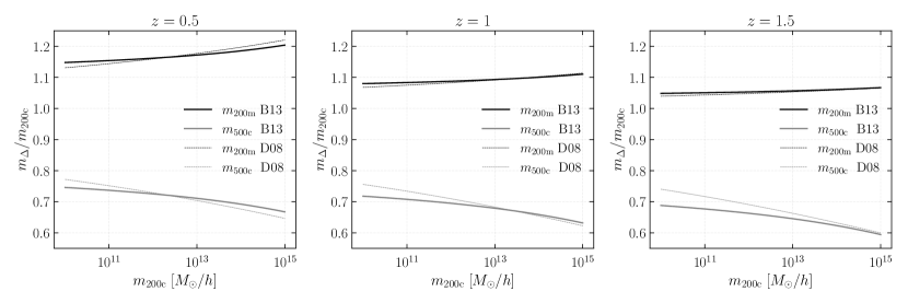
B.7 Mass Conversions

Although here we exclusively used the $m_{200\mathrm{c}}$ mass definition, we explain how to convert between mass definition as it can be useful for comparison with other analyses or to implement different mass functions, HOD’s and tracer profiles. To convert between $m_{\Delta}$ and $m_{\Delta^{\prime}}$, we compute $m_{\Delta^{\prime}}=\int_{0}^{r_{\Delta^{\prime}}}\mathrm{d}r4\pi r^{2}\rho_{{}_{\mathrm{NFW}}}(r)$ with the NFW profile defined in terms of $r_{s}=r_{\Delta}/c_{\Delta}$. Its expression is equivalent to

$$\frac{m_{\Delta^{\prime}}}{m_{\Delta}}-\frac{f_{{}_{\mathrm{NFW}}}(c_{\Delta})}{f_{{}_{\mathrm{NFW}}}(c_{\Delta}r_{\Delta^{\prime}}/r_{\Delta})}=0\quad\mathrm{with}\quad r_{\Delta^{\prime}}=\left[3m_{\Delta}/(4\pi\Delta^{\prime}\rho_{\mathrm{crit}}(z))\right]^{1/3}$$ (B26)

which can be solved for $m_{\Delta^{\prime}}$ with a root-finding algorithm. In class_sz we use Brent’s method (Brent, 1973). For reference, we show the conversions between $m_{\mathrm{200c}}$, $m_{\mathrm{200m}}$ and $m_{\mathrm{500c}}$ at three redshifts for the Bhattacharya et al. (2013) and Duffy et al. (2008) concentration-mass relations in Figure 16. Overall, $m_{\mathrm{200m}}$ is $\approx 5-20\%$ larger than $m_{\mathrm{200c}}$, while $m_{\mathrm{500c}}$ is $\approx 20-40\%$ lower than $m_{\mathrm{200c}}$. The Bhattacharya et al. (2013) and Duffy et al. (2008) agree well at high masses but differ substantially at low masses.

B.8 Galaxy Halo Occupation Distributions

Galaxies populate dark matter halos in complicated ways. Its simple and faithful description, galaxy Halo Occupation Distributions (HOD) was proposed in Zheng et al. (2007). Here we use a slightly different parameterization, to match that of Zacharegkas et al. (2021). The expectation value for number of central galaxies in a halo of mass $m$ is given by

$$N_{\mathrm{cent}}(m)=\frac{1}{2}\left(1+\mathrm{erf}\left[\frac{\log_{10}(m/m_{\mathrm{min}})}{\sigma_{\mathrm{log}_{10}m}}\right]\right)$$ (B27)

where $m_{\mathrm{min}}$ is a pivot mass above which, on average, halos have a central galaxy. Here, $\sigma_{\mathrm{log}_{10}m}$ controls the steepness of the transition in mass from no galaxy to having at least one galaxy in the halo. The expectation value for number of satellite galaxies is a power law with an exponent $\alpha_{s}$,

$$N_{\mathrm{sat}}(m)=N_{\mathrm{cent}}(m)\left(\frac{m}{m_{1}}\right)^{\alpha_{s}},$$ (B28)

where $m_{\mathrm{1}}$ is a pivot mass above which the number of satellites increases steeply. In our fiducial model, corresponding to the best-fit to blue unWISE galaxies, these parameters are set to $m_{\mathrm{min}}=1.01\times 10^{13}{M_{\odot}}/h$, $m_{1}=1.18\times 10^{14}{M_{\odot}}/h$, $\alpha_{s}=2.08$ and $\sigma_{\mathrm{log}_{10}m}=0.76$ (see Kusiak et al., 2022, for details).

Given a specific HOD (Eq. B27 and B28) we can compute the galaxy number density and galaxy bias at $z$ as

$$\bar{n}_{\mathrm{g}}(z)=\langle N_{\mathrm{cent}}+N_{\mathrm{sat}}\rangle_{n},\quad\mathrm{with}\quad b_{\mathrm{g}}(z)=\frac{1}{\bar{n}_{\mathrm{g}}(z)}\langle b^{(1)}(N_{\mathrm{cent}}+N_{\mathrm{sat}})\rangle_{n},$$ (B29)

where $b^{(1)}$ is the linear bias of Eq. (B13). As for the spatial distribution, central galaxies are naturally assumed to be located at the center of halos (their density profile is a Dirac delta function) and satellite galaxies are assumed to be randomly distributed along an NFW-like radial profile. Thus, the Fourier transform of the galaxy density profile is

$$\hat{u}^{\mathrm{g}}_{k}=\frac{1}{\bar{n}_{\mathrm{g}}}\left(N_{\mathrm{cent}}+N_{\mathrm{sat}}\hat{u}^{\mathrm{sat}}_{k}\right)$$ (B30)

where $\hat{u}^{\mathrm{sat}}_{k}$ is the same Eq. (B24) with $\lambda=1$ and without the ${m_{\lambda r_{\Delta}}}/{\rho_{\mathrm{m},0}}$ prefactor. In addition, $c_{\Delta}$ is often replaced by a free parameter $c_{\mathrm{sat}}$ to allow for more freedom in the radial distribution. Another important HOD quantity is the Fourier transform of the second moment of the satellites galaxy distribution:

$$\hat{u}^{\mathrm{gg}}_{k}=\frac{1}{\bar{n}_{\mathrm{g}}^{2}}\left[N_{\mathrm{sat}}^{2}(\hat{u}^{\mathrm{sat}}_{k})^{2}+2N_{\mathrm{sat}}\hat{u}^{\mathrm{sat}}_{k}\right],$$ (B31)

(see, e.g., van den Bosch et al., 2013; Koukoufilippas et al., 2020), as it determines the 1-halo term of the galaxy power spectrum.

Figure 17: Left: The matter power spectrum at $z=1$ computed in the halo model (1-halo term is the solid black line, 2-halo term is the dash-dotted black line, and sum is the thick solid line) compared with the halofit formula (dotted blue line) Takahashi et al. (2012) and the hmcode prediction (dashed orange) Mead et al. (2021). The thick grey line shows the halo model prediction when the consistency prescriptions of Subsection B.2 are not taken into account. Middle: The power spectrum of baryons in the halo model for two different density profile types (Adiabatic and AGN Feedback) and rescaled by $1/f_{b}^{2}$ compared with the halofit matter power spectrum. Right: Galaxy power spectrum in the halo model (black lines) at $z=1$ compared with the matter power spectrum computed with halofit (dotted blue line) and the halofit power spectrum times $b_{\mathrm{g}}^{2}$ squared (dashed blue) with $b_{\mathrm{g}}$ from Eq. (B29).

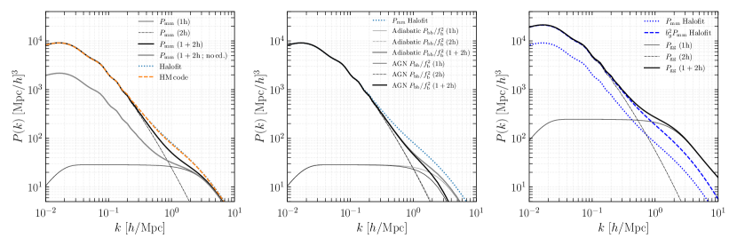
B.9 Application to Tracers

In this Section we present explicit expressions for 3D auto-power spectra of tracers in the halo-model. Cross-power spectra expressions are easily obtained in a similar fashion.

B.9.1 Cold Dark Matter

When CDM density is assumed to follow the NFW profile (see Appendix B.6), the halo model matter power spectrum at $z$ is $P^{\mathrm{hm}}_{\delta_{\mathrm{m}}\delta_{\mathrm{m}}}=P_{\delta_{\mathrm{m}}\delta_{\mathrm{m}}}^{\mathrm{1h}}+P_{\delta_{\mathrm{m}}\delta_{\mathrm{m}}}^{\mathrm{2h}}$ with

$$P_{\delta_{\mathrm{m}}\delta_{\mathrm{m}}}^{\mathrm{1h}}(k,\chi)=\langle\hat{u}^{{}_{\mathrm{NFW}}}_{k}\hat{u}^{{}_{\mathrm{NFW}}}_{k}\rangle_{n}\quad\mathrm{and}\quad P_{\delta_{\mathrm{m}}\delta_{\mathrm{m}}}^{\mathrm{2h}}(k,\chi)=\langle b^{(1)}\hat{u}^{{}_{\mathrm{NFW}}}_{k}\rangle_{n}^{2}P_{L}(k,\chi)$$ (B32)

where $P_{L}$ is the linear matter power spectrum. In the low-$k$ limit we have $\langle b^{(1)}\hat{u}^{{}_{\mathrm{NFW}}}_{k}\rangle_{n}\rightarrow 1$ (by construction and consistency) so that $P_{\delta_{\mathrm{m}}\delta_{\mathrm{m}}}^{\mathrm{2h}}\sim P_{L}$, whereas $P_{\delta_{\mathrm{m}}\delta_{\mathrm{m}}}^{\mathrm{1h}}\sim\langle m_{\Delta}^{2}/\rho_{\mathrm{m,0}}^{2}\rangle$ which is independent of $k$. Hence, at low-$k$ the 2-halo term dominates and we have $P^{\mathrm{hm}}_{\delta_{\mathrm{m}}\delta_{\mathrm{m}}}\sim P_{L}$. The halo model matter power spectrum is plotted on the left panel of Figure 17 against the halofit and hmcode (which are nearly identical). The mismatch between the halo model power spectrum and the N-body calibrated formulas (halofit and hmcode) in the transition regime between the 2-halo and 1-halo term is a well-known short-coming of the halo model. This issue has been addressed in several manners. For instance, Mead et al. (2015) suggest using $P^{\mathrm{hm}}_{\delta_{\mathrm{m}}\delta_{\mathrm{m}}}=[(P^{\mathrm{1h}}_{\delta_{\mathrm{m}}\delta_{\mathrm{m}}})^{\alpha}+(P^{\mathrm{2h}}_{\delta_{\mathrm{m}}\delta_{\mathrm{m}}})^{\alpha})]^{1/\alpha}$ where $\alpha$ is a free parameter. Another approach, proposed in Philcox et al. (2020) is to use perturbation theory at one-loop order in the modeling of the 2-halo term, amounting to replace $P_{L}$ in Eq. (B32) by $P_{NL}=P_{L}+P_{\mathrm{spt}}+P_{\mathrm{ct}}$ where $P_{\mathrm{spt}}=P_{22}+P_{13}$ with $P_{22}$ and $P_{13}$ resulting from higher-order terms associated with the $F_{2}$ and $F_{3}$ coupling kernels (see, e.g., Bernardeau et al., 2002) and $P_{\mathrm{ct}}(k)=-c_{\mathrm{s}}^{2}k^{2}P_{L}(k)$ with $c_{\mathrm{s}}$ a free parameter of the model. What these approaches have in common is inclusion of the nuisance parameters to the model. The extra nuisance parameters then need to be calibrated on simulations or marginalized over. Here we do not study these extra pieces of modelling for the transition regimes and leave them for future work.

B.9.2 Electrons

The electron power spectrum is computed in the halo model using the Fourier transform of the gas density profile, $\hat{u}^{\mathrm{e}}$ of Eq. (46), as

$$P_{\delta_{\mathrm{e}}\delta_{\mathrm{e}}}^{\mathrm{1h}}(k,\chi)=\langle\hat{u}^{\mathrm{e}}_{k}\hat{u}^{\mathrm{e}}_{k}\rangle_{n}\quad\mathrm{and}\quad P_{\delta_{\mathrm{e}}\delta_{\mathrm{e}}}^{\mathrm{2h}}(k,\chi)=\langle b^{(1)}\hat{u}^{\mathrm{e}}_{k}\rangle_{n}^{2}P_{L}(k,\chi).$$ (B33)

The gas density profile is normalized such that

$$\lim_{k\rightarrow 0}\hat{u}^{\mathrm{e}}_{k}=f_{\mathrm{b}}f_{\mathrm{free}}\frac{m_{\Delta}}{\rho_{\mathrm{m,0}}},$$ (B34)

and there for in the low-$k$ limit we have $P_{\delta_{\mathrm{e}}\delta_{\mathrm{e}}}^{\mathrm{hm}}\approx P_{\delta_{\mathrm{e}}\delta_{\mathrm{e}}}^{\mathrm{2h}}\approx f_{\mathrm{b}}^{2}P_{L}$, irrespective of the gas density profile assumption. In the high-$k$ regime, the difference between the gas density profile and the NFW profile can be significant and therefore the scale dependence of the baryon power spectrum can depart from that of the non-linear matter power spectrum. This is illustrated in the middle panel of Figure 17.

B.9.3 Galaxies

The galaxy power spectrum is $P_{\delta_{\mathrm{g}}\delta_{\mathrm{g}}}^{\mathrm{hm}}=P_{\delta_{\mathrm{g}}\delta_{\mathrm{g}}}^{\mathrm{SN}}+P_{\delta_{\mathrm{g}}\delta_{\mathrm{g}}}^{\mathrm{1h}}+P_{\delta_{\mathrm{g}}\delta_{\mathrm{g}}}^{\mathrm{2h}}$, where $P_{\delta_{\mathrm{g}}\delta_{\mathrm{g}}}^{\mathrm{SN}}$ is the shot-noise contribution, whose expression is

$$P_{\delta_{\mathrm{g}}\delta_{\mathrm{g}}}^{\mathrm{SN}}=\frac{1}{\bar{n}_{\mathrm{g}}},$$ (B35)

where $\bar{n}_{\mathrm{g}}$ is defined in Eq. (B29). The 1- and 2-halo terms are

$$P_{\delta_{\mathrm{g}}\delta_{\mathrm{g}}}^{\mathrm{1h}}=\langle\hat{u}^{\mathrm{gg}}_{k}\rangle_{n}\quad\mathrm{and}\quad P_{\delta_{\mathrm{g}}\delta_{\mathrm{g}}}^{\mathrm{2h}}=\langle b^{(1)}\hat{u}^{\mathrm{g}}_{k}\rangle_{n}^{2}P_{L}(k,\chi),$$ (B36)

respectively, where $\hat{u}^{\mathrm{gg}}_{k}$ and $\hat{u}^{\mathrm{g}}_{k}$ are defined in Eq. (B31) and (B30). In the low-$k$ limit, since $\hat{u}^{\mathrm{sat}}_{k}\approx 1$, we have $\langle b^{(1)}\hat{u}^{\mathrm{g}}_{k}\rangle_{n}\rightarrow b_{\mathrm{g}}(z)$ and thus $P_{\delta_{\mathrm{g}}\delta_{\mathrm{g}}}^{\mathrm{hm}}\approx b_{\mathrm{g}}^{2}P_{L}$. In the high-$k$ regime, the scale dependence is determined by the HOD and departs from that of the halofit power spectrum, as can be seen on the right panel of Figure 17.

In fact, the observed power spectrum of galaxies includes an extra contributions coming from lensing magnification. We have

$$\delta_{\mathrm{g}}^{\mathrm{obs}}=\delta_{\mathrm{g}}+\mu_{\mathrm{g}}\quad\mathrm{with}\quad\mu_{\mathrm{g}}=(5s-2)\delta_{\mathrm{m}}\quad\mathrm{and}\quad s\equiv\frac{\mathrm{dlog_{10}N}}{\mathrm{d}\mathcal{M}}$$ (B37)

where $\mathcal{M}$ is the apparent magnitude of the galaxies, evaluated near the magnitude limit of the survey. The extra-contributions are $P_{\mathrm{\delta_{g}\mu_{g}}}^{\mathrm{hm}}=(5s-2)P_{\mathrm{\delta_{g}\delta_{m}}}^{\mathrm{hm}}$ and $P_{\mathrm{\mu_{g}\mu_{g}}}^{\mathrm{hm}}=(5s-2)^{2}P_{\mathrm{\delta_{m}\delta_{m}}}^{\mathrm{hm}}$.

B.9.4 Useful Angular Power Spectra

Angular power spectra are obtained from the 3D power spectra using Eq. (B19). Each tracer has its own projection kernel. For the kSZ effect, $W^{\mathrm{kSZ}}$ is given in Eq. (24) along with the angular power spectrum expression in the high-$k$ limit. We show the kSZ angular power spectrum in Figure 18 for different gas profile assumptions. The low-$\ell$ limit does not depend on the assumption. The halo model power spectrum computed with the AGN Feedback gas profile agrees reasonably well with results from simulations (Battaglia et al., 2010b).

For CMB lensing, the projection kernel is

$$W^{\mathrm{\kappa_{{}_{CMB}}}}(\chi)=\frac{3}{2}\frac{\Omega_{\mathrm{m}}(H_{0}/c)^{2}}{\chi^{2}}(1+z)\chi\frac{\chi_{\star}-\chi}{\chi_{\star}}.$$ (B38)

where $\chi_{\star}$ is the comoving distance to last scattering.

For galaxy weak lensing, the projection kernel is

$$W^{\mathrm{\kappa_{{}_{g}}}}(\chi)=\frac{3}{2}\frac{\Omega_{\mathrm{m}}(H_{0}/c)^{2}}{\chi^{2}}(1+z)\chi I_{s}(\chi)\quad\mathrm{with}\quad I_{s}(\chi)=\int_{z}^{+\infty}\mathrm{d}z_{\mathrm{s}}\varphi^{\prime}_{s}(z_{\mathrm{s}})\frac{\chi_{s}-\chi}{\chi_{s}}$$ (B39)

where $\varphi^{\prime}_{s}$ is the normalized redshift distribution of source galaxies, and we used the notation $\chi_{s}=\chi(z_{\mathrm{s}})$ for the comoving distance to redshift $z_{\mathrm{s}}$. (Note that, formally, Eq. (B39) reduces to Eq. (B38) if $\varphi^{\prime}(z_{\mathrm{s}})=\delta_{D}(z_{\mathrm{s}}-z_{\star})$.).

For galaxy number density, the projection kernel is

$$W^{\delta_{\mathrm{g}}}(\chi)=\frac{H}{\chi^{2}c}\varphi_{\mathrm{g}}^{\prime}(z)\quad\mathrm{with}\quad\varphi_{\mathrm{g}}^{\prime}(z)=\frac{1}{N_{\mathrm{g}}^{\mathrm{tot}}}\frac{\mathrm{d}N_{\mathrm{g}}}{\mathrm{d}z}\quad\mathrm{where}\quad N_{\mathrm{g}}^{\mathrm{tot}}=\int\mathrm{d}z\frac{\mathrm{d}N_{\mathrm{g}}}{\mathrm{d}z}.$$ (B40)

Here, $\frac{\mathrm{d}N_{\mathrm{g}}}{\mathrm{d}z}$ is the galaxy redshift distribution of the survey which is from data. For lensing magnification, the projection kernel is

$$W^{\mathrm{\mu_{{}_{g}}}}(\chi)=\frac{3}{2}\frac{\Omega_{\mathrm{m}}(H_{0}/c)^{2}}{\chi^{2}}(1+z)\chi I_{\mathrm{g}}(\chi)\quad\mathrm{with}\quad I_{\mathrm{g}}(\chi)=\int_{z}^{+\infty}\mathrm{d}z_{g}\varphi^{\prime}_{\mathrm{g}}(z_{\mathrm{g}})\frac{\chi_{\mathrm{g}}-\chi}{\chi_{\mathrm{g}}}.$$ (B41)

where $\varphi^{\prime}_{\mathrm{g}}$ is the normalized redshift distribution of lens galaxies, and we used the notation $\chi_{\mathrm{g}}=\chi(z_{\mathrm{g}})$ for the comoving distance to redshift $z_{\mathrm{g}}$. in Figure 19 we show a comparison of CMB angular power power spectra computed with the halo-model and the halofit power spectrum. The noise curves for SO and S4 are also plotted.

Figure 18: The dimensionless angular power spectrum of the kSZ effect from hydrodynamical simulations and using the halo model formula in the high-$k$ regime (see Eq. 24). For the halo model results we assumed the gas distributed according the AGN Feedback model (red solid lines) and NFW-like profile (purple line). The simulation results are the thick dashed lines and are from Battaglia et al. (2010b). The black dashed line represents the contribution from halos while the grey dashed line is the contribution from reionization (it is not used in our analysis, but shown here for comparison).

Figure 19: Dimensionless angular power spectrum of CMB lensing convergence with noise estimates for SO and S4. The red dotted line shows the class prediction which is based on halofit. The black lines are the class_sz predictions using halo model (solid, dashed and dashed-dotted lines) and halofit (thin dashed line). Note that for this plot we used $z_{\mathrm{max}}=15$.

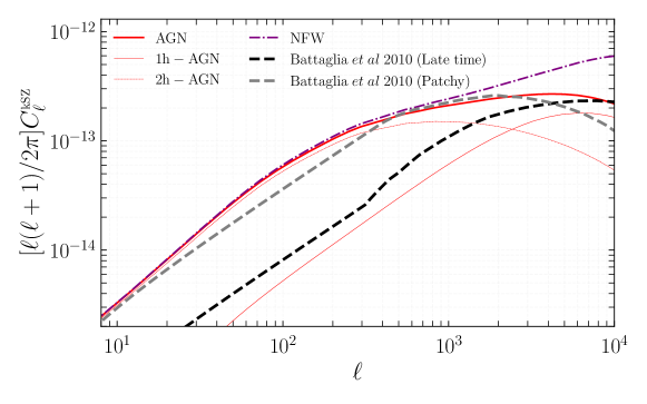
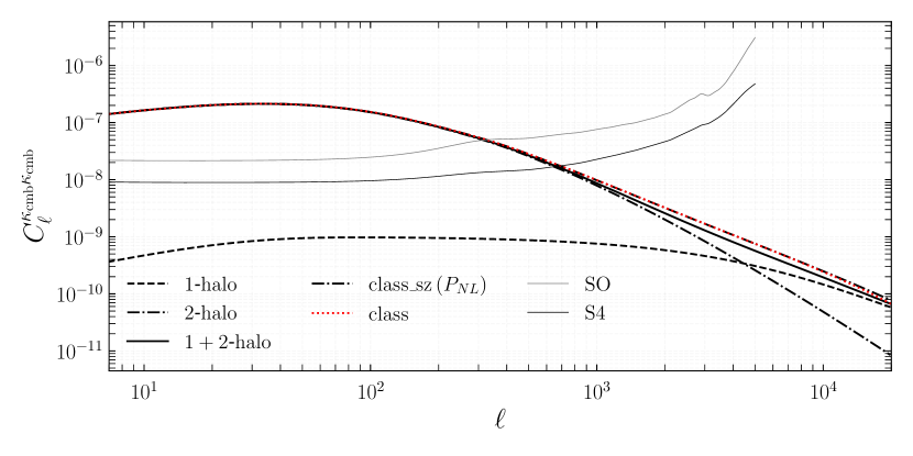
Appendix C Comparison with Previous Works

C.1 Choices of Wiener Filter

Figure 20: Comparison of Wiener filters (multiplied by the respective beams).

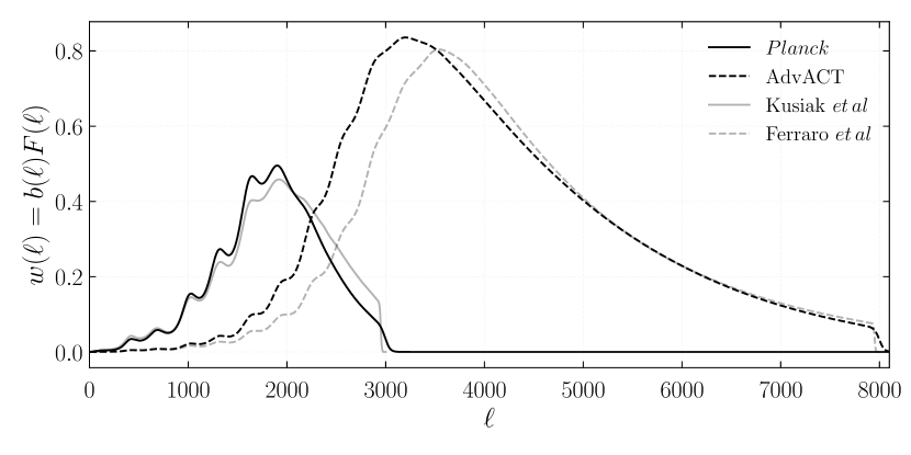
In all previous works using the projected-field kSZ estimator, the filter ansatz was

$$w^{\mathrm{prev.}}(\ell)=b(\ell)\frac{C_{\ell}^{\mathrm{kSZ}}}{C_{\ell}^{\mathrm{tot}}}.$$ (C1)

This differs from our filter definition (see Eq. 25) as we use a square root in the numerator. These two choices yield similar SNR, but the version with the square root is always better, yielding larger SNRs by $\approx 3-5\%$.

To justify the filter definition of Eq. (25) we provide a heuristic derivation based on Appendix B of Smith et al. (2007). Since the projected field kSZ power spectrum is an integral over the bispectrum, we expect the optimal estimator to be similar to the optimal bispectrum estimator. In general, the optimal bispectrum estimator is given by

$$\hat{\mathcal{C}}=\frac{1}{F}(\hat{\mathcal{C}}_{3}-\hat{\mathcal{C}_{1}}),$$ (C2)

where $F$ is a normalization (whose exact expression is not important here) and where $\hat{\mathcal{C}}_{3}$ and $\hat{\mathcal{C}}_{1}$ are a three-point and one-point term. The one-point term can be significant when the sky coverage is partial and the noise is inhomogeneous, but we can omit it for the purpose of this discussion. The three-point term contains the scale-dependent information we are interested in. It is given by

$$\hat{\mathcal{C}}_{3}\approx\sum_{\ell_{i},m_{i}}B_{\ell_{1}\ell_{2}\ell_{3}}\mathcal{G}_{m_{1}m_{2}m_{3}}^{\ell_{1}\ell_{2}\ell_{3}}\tilde{a}_{\ell_{1}m_{1}}\tilde{a}_{\ell_{2}m_{2}}\tilde{X}_{\ell_{3}m_{3}}$$ (C3)

where $B$ is the theoretical/predicted hybrid bispectrum, $\mathcal{G}$ is a Wigner-$3j$ symbol (see Eq. 6 of Smith et al., 2007) and the tilde fields $\tilde{a}$ and $\tilde{X}$ are the harmonic coefficients of inverse-variance weighted CMB and LSS maps, i.e.,

$$\tilde{a}_{\ell m}=(C_{\ell}^{\Theta\Theta}+C_{\ell}^{\mathrm{kSZ}}+N_{\ell}^{\Theta\Theta})^{-1}a_{\ell m},\quad\mathrm{and}\quad\tilde{X}_{\ell m}=(C_{\ell}^{XX}+N_{\ell}^{XX})^{-1}X_{\ell m}.$$ (C4)

The inverse variance weighting ensures that the poorly measured modes are filtered out and hence contribute less to the variance of the estimator. From Eq. (C3) we see that the optimal filter $w_{\ell_{1}}$ to apply to the temperature map $a_{\ell_{1}m_{1}}$ should have the scale dependence of $B_{\ell_{1}\ell_{2}\ell_{3}}/C_{\ell_{1}}^{\mathrm{tot}}$. Since the term that contributes most to the bispectrum in the range of scales of interest here is the 1-halo term, we can approximate the scale dependence as

$$w_{\ell_{1}}\sim\frac{1}{C_{\ell_{1}}^{\mathrm{tot}}}\int\mathrm{d}n_{1}\hat{u}_{\ell_{1}}^{\mathrm{e}}(m_{1})\hat{u}_{\ell_{2}}^{\mathrm{e}}(m_{1})\hat{u}_{\ell_{3}}^{X}(m_{1})\sim\frac{\sqrt{C_{\ell_{1}}^{\mathrm{kSZ}}}}{C_{\ell_{1}}^{\mathrm{tot}}}.$$ (C5)

C.2 Comparison with forecats from Ferraro et al.

Figure 21: Projected-field kSZ power spectrum in cross-correlation with galaxy density assuming Planck$\times$WISE (left) and AdvACT$\times$WISE (right). The solid lines with error bars are the class_sz predictions for the power spectrum and covariance matrix and the dashed lines are computed with an independent code that was used in (Ferraro et al., 2016; Hill et al., 2016; Kusiak et al., 2021). Here the computations are done within the effective approach (see Subsection 2.4), using the the filters of Figure 20 (grey lines).

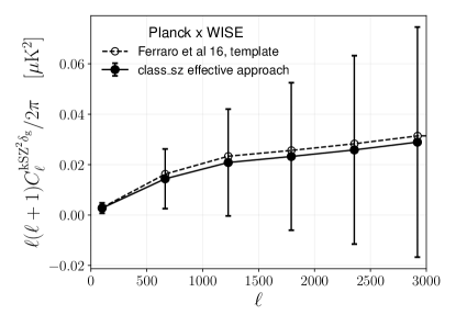
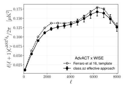
We compared our effective approach calculations with the code used in Ferraro et al. (2016); Hill et al. (2016); Kusiak et al. (2021). We found a good agreement over all scales for Planck$\times$WISE and AdvACT$\times$WISE (relative difference of $\approx$10%). For this comparison we used the same settings as in Ferraro et al. (2016). In particular, we used the filters labeled ‘Kusiak et al’ and ‘Ferraro et al’ in Figure 20, a sky fraction $f_{\mathrm{sky}}$, an effective galaxy bias $b_{\mathrm{g}}^{\mathrm{eff}}=1.13$, the linear matter power spectrum in the velocity dispersion, and the normalized galaxy redshift distribution of Figure 10 of Ferraro et al. (2016). For the covariance matrix calculation we used a shot noise of $C_{\ell}^{\mathrm{SN}}=1.26\times 10^{-7}$ (which corresponds to 50 million galaxies over half the sky). The power spectra are plotted together on Figure 21.

Ferraro et al. (2016) presented SNR forecasts that differ from the ones we obtained in Section 4. For AdvACT$\times$WISE they obtained an SNR on $f_{\mathrm{free}}$ of 232. In the same settings as them (see paragraph above) we get nearly the same estimate, finding 223. This is roughly six times larger than our most optimistic forecast with AdvACT$\times$unWISE (note that the SNR on $f_{\mathrm{free}}$ is two times $\mathrm{SNR_{tot}}$ if we do not take into account degeneracies with HOD parameters and assume the galaxy bias to be tightly constrained). This significant difference is mainly explained by the fact that the filter in Ferraro et al. (2016) uses a $10\,\mu\mathrm{K}$-arcmin pixel noise level while we use $20\,\mu\mathrm{K}$-arcmin (which is more consistent with current ILC noise estimates) and that our fiducial model for the projected-field kSZ power spectrum assumes the AGN Feedback gas density profile whereas Ferraro et al. (2016) uses the effective approach calculation. The difference of filter and the difference of fiducial model change the SNR by roughly the same amount.

References

- Abazajian et al. (2019) Abazajian, K., Addison, G., Adshead, P., et al. 2019, arXiv e-prints, arXiv:1907.04473. https://arxiv.org/abs/1907.04473
- Abbott et al. (2018) Abbott, T., Abdalla, F., Alarcon, A., et al. 2018, Physical Review D, 98, doi: 10.1103/physrevd.98.043526
- Adam et al. (2017) Adam, R., Bartalucci, I., Pratt, G. W., et al. 2017, Astronomy & Astrophysics, 598, A115, doi: 10.1051/0004-6361/201629182
- Ade et al. (2019) Ade, P., Aguirre, J., Ahmed, Z., et al. 2019, J. Cosmology Astropart. Phys, 2019, 056, doi: 10.1088/1475-7516/2019/02/056
- Aiola et al. (2020) Aiola, S., Calabrese, E., Maurin, L., et al. 2020, J. Cosmology Astropart. Phys, 2020, 047, doi: 10.1088/1475-7516/2020/12/047
- Alonso et al. (2016) Alonso, D., Louis, T., Bull, P., & Ferreira, P. G. 2016, Phys. Rev. D, 94, 043522, doi: 10.1103/PhysRevD.94.043522
- Alvarez (2016) Alvarez, M. A. 2016, The Astrophysical Journal, 824, 118, doi: 10.3847/0004-637x/824/2/118
- Amodeo et al. (2021) Amodeo, S., Battaglia, N., Schaan, E., et al. 2021, Physical Review D, 103, doi: 10.1103/physrevd.103.063514
- Amon & Efstathiou (2022) Amon, A., & Efstathiou, G. 2022. https://arxiv.org/abs/2206.11794
- Audren et al. (2013) Audren, B., Lesgourgues, J., Benabed, K., & Prunet, S. 2013, JCAP, 1302, 001, doi: 10.1088/1475-7516/2013/02/001
- Battaglia (2016) Battaglia, N. 2016, J. Cosmology Astropart. Phys, 2016, 058, doi: 10.1088/1475-7516/2016/08/058
- Battaglia et al. (2010a) Battaglia, N., Bond, J. R., Pfrommer, C., Sievers, J. L., & Sijacki, D. 2010a, The Astrophysical Journal, 725, 91–99, doi: 10.1088/0004-637x/725/1/91
- Battaglia et al. (2010b) —. 2010b, The Astrophysical Journal, 725, 91–99, doi: 10.1088/0004-637x/725/1/91
- Battaglia et al. (2019) Battaglia, N., Hill, J. C., Amodeo, S., et al. 2019, Probing Feedback in Galaxy Formation with Millimeter-wave Observations, arXiv, doi: 10.48550/ARXIV.1903.04647
- Bernardeau et al. (2002) Bernardeau, F., Colombi, S., Gaztañaga, E., & Scoccimarro, R. 2002, Physics Reports, 367, 1–248, doi: 10.1016/s0370-1573(02)00135-7
- Bernardis et al. (2017) Bernardis, F. D., Aiola, S., Vavagiakis, E., et al. 2017, Journal of Cosmology and Astroparticle Physics, 2017, 008, doi: 10.1088/1475-7516/2017/03/008
- Bhattacharya et al. (2013) Bhattacharya, S., Habib, S., Heitmann, K., & Vikhlinin, A. 2013, ApJ, 766, 32, doi: 10.1088/0004-637X/766/1/32
- Birkinshaw (1999) Birkinshaw, M. 1999, Physics Reports, 310, 97, doi: 10.1016/s0370-1573(98)00080-5
- Birkinshaw et al. (1984) Birkinshaw, M., Gull, S. F., & Hardebeck, H. 1984, Nature, 309, 34, doi: 10.1038/309034a0
- Blanchard et al. (2020) Blanchard, A., Camera, S., Carbone, C., et al. 2020, Astronomy & Astrophysics, 642, A191, doi: 10.1051/0004-6361/202038071
- Blas et al. (2011) Blas, D., Lesgourgues, J., & Tram, T. 2011, Journal of Cosmology and Astroparticle Physics, 2011, 034–034, doi: 10.1088/1475-7516/2011/07/034
- Bobin et al. (2016) Bobin, J., Sureau, F., & Starck, J. L. 2016, A&A, 591, A50, doi: 10.1051/0004-6361/201527822
- Bocquet et al. (2020) Bocquet, S., Heitmann, K., Habib, S., et al. 2020, The Mira-Titan Universe. III. Emulation of the Halo Mass Function, arXiv, doi: 10.48550/ARXIV.2003.12116
- Bocquet et al. (2019) Bocquet, S., Dietrich, J. P., Schrabback, T., et al. 2019, The Astrophysical Journal, 878, 55, doi: 10.3847/1538-4357/ab1f10
- Bolliet et al. (2020) Bolliet, B., Brinckmann, T., Chluba, J., & Lesgourgues, J. 2020, Monthly Notices of the Royal Astronomical Society, 497, 1332, doi: 10.1093/mnras/staa1835
- Bolliet et al. (2018) Bolliet, B., Comis, B., Komatsu, E., & Macías-Pérez, J. F. 2018, Mon. Not. Roy. Astron. Soc., 477, 4957, doi: 10.1093/mnras/sty823
- Bond et al. (1991) Bond, J. R., Cole, S., Efstathiou, G., & Kaiser, N. 1991, ApJ, 379, 440, doi: 10.1086/170520
- Brent (1973) Brent, R. 1973, Algorithms for minimization without derivatives (Prentice-Hall)
- Brinckmann & Lesgourgues (2018) Brinckmann, T., & Lesgourgues, J. 2018. https://arxiv.org/abs/1804.07261
- Bryan & Norman (1998) Bryan, G. L., & Norman, M. L. 1998, 495, 80, doi: 10.1086/305262
- Bull et al. (2012) Bull, P., Clifton, T., & Ferreira, P. G. 2012, Physical Review D, 85, doi: 10.1103/physrevd.85.024002
- Calafut et al. (2021) Calafut, V., Gallardo, P., Vavagiakis, E., et al. 2021, Physical Review D, 104, doi: 10.1103/physrevd.104.043502
- Carlstrom et al. (2002) Carlstrom, J. E., Holder, G. P., & Reese, E. D. 2002, Annual Review of Astronomy and Astrophysics, 40, 643, doi: 10.1146/annurev.astro.40.060401.093803
- Cayuso et al. (2021) Cayuso, J., Bloch, R., Hotinli, S. C., Johnson, M. C., & McCarthy, F. 2021. https://arxiv.org/abs/2111.11526
- Chen et al. (2022) Chen, N., Trac, H., Mukherjee, S., & Cen, R. 2022. https://arxiv.org/abs/2203.04337
- Chiang et al. (2020) Chiang, Y.-K., Makiya, R., Mé nard, B., & Komatsu, E. 2020, The Astrophysical Journal, 902, 56, doi: 10.3847/1538-4357/abb403
- Chisari et al. (2019) Chisari, N. E., et al. 2019, Astrophys. J. Suppl., 242, 2, doi: 10.3847/1538-4365/ab1658
- Chluba & Sunyaev (2011) Chluba, J., & Sunyaev, R. A. 2011, Monthly Notices of the Royal Astronomical Society, 419, 1294–1314, doi: 10.1111/j.1365-2966.2011.19786.x
- Choi et al. (2020) Choi, S. K., Hasselfield, M., Ho, S.-P. P., et al. 2020, Journal of Cosmology and Astroparticle Physics, 2020, 045, doi: 10.1088/1475-7516/2020/12/045
- Chown et al. (2018) Chown, R., et al. 2018, Astrophys. J. Suppl., 239, 10, doi: 10.3847/1538-4365/aae694
- Contreras et al. (2022) Contreras, D., McCarthy, F., & Johnson, M. C. 2022. https://arxiv.org/abs/2205.15779
- Cooray (2001) Cooray, A. 2001, Phys. Rev. D, 64, 063514, doi: 10.1103/PhysRevD.64.063514
- Cooray & Sheth (2002) Cooray, A., & Sheth, R. K. 2002, Phys. Rept., 372, 1, doi: 10.1016/S0370-1573(02)00276-4
- Coulton et al. (2020) Coulton, W. R., Meerburg, P. D., Baker, D. G., et al. 2020, Physical Review D, 101, doi: 10.1103/physrevd.101.123504
- Crawford et al. (2014) Crawford, T. M., Schaffer, K. K., Bhattacharya, S., et al. 2014, ApJ, 784, 143, doi: 10.1088/0004-637X/784/2/143
- de Graaff et al. (2019) de Graaff, A., Cai, Y.-C., Heymans, C., & Peacock, J. A. 2019, Astronomy & Astrophysics, 624, A48, doi: 10.1051/0004-6361/201935159
- DeDeo et al. (2005) DeDeo, S., Spergel, D. N., & Trac, H. 2005, arXiv e-prints, astro. https://arxiv.org/abs/astro-ph/0511060
- Deutsch et al. (2018) Deutsch, A.-S., Dimastrogiovanni, E., Johnson, M. C., Münchmeyer, M., & Terrana, A. 2018, Physical Review D, 98, doi: 10.1103/physrevd.98.123501
- Dodelson & Schmidt (2020) Dodelson, S., & Schmidt, F. 2020, Modern Cosmology (Elsevier Science). https://books.google.com/books?id=GGjfywEACAAJ
- Dolag et al. (2016) Dolag, K., Komatsu, E., & Sunyaev, R. 2016, Monthly Notices of the Royal Astronomical Society, 463, 1797, doi: 10.1093/mnras/stw2035
- Doré et al. (2004) Doré, O., Hennawi, J. F., & Spergel, D. N. 2004, ApJ, 606, 46, doi: 10.1086/382946
- Duffy et al. (2008) Duffy, A. R., Schaye, J., Kay, S. T., & Dalla Vecchia, C. 2008, Monthly Notices of the Royal Astronomical Society: Letters, 390, L64–L68, doi: 10.1111/j.1745-3933.2008.00537.x
- Eisenstein et al. (2011) Eisenstein, D. J., Weinberg, D. H., Agol, E., et al. 2011, AJ, 142, 72, doi: 10.1088/0004-6256/142/3/72
- Ferraro et al. (2016) Ferraro, S., Hill, J. C., Battaglia, N., Liu, J., & Spergel, D. N. 2016, Phys. Rev. D, 94, 123526, doi: 10.1103/PhysRevD.94.123526
- Ferraro & Smith (2018) Ferraro, S., & Smith, K. M. 2018, Physical Review D, 98, doi: 10.1103/physrevd.98.123519
- Ferreira et al. (1999) Ferreira, P. G., Davis, M., Feldman, H. A., Jaffe, A. H., & Juszkiewicz, R. 1999, Measuring Omega with Galaxy Streaming Velocities, arXiv, doi: 10.48550/ARXIV.ASTRO-PH/9904074
- Flender et al. (2017) Flender, S., Nagai, D., & McDonald, M. 2017, The Astrophysical Journal, 837, 124, doi: 10.3847/1538-4357/aa60bf
- Frigo & Johnson (2005) Frigo, M., & Johnson, S. G. 2005, Proceedings of the IEEE, 93, 216
- Fry (1984) Fry, J. N. 1984, ApJ, 279, 499, doi: 10.1086/161913
- Galassi (2018) Galassi, M. e. a. 2018, GNU Scientific Library Reference Manual. https://www.gnu.org/software/gsl/
- Gatti et al. (2021) Gatti, M., Pandey, S., Baxter, E., et al. 2021, arXiv e-prints, arXiv:2108.01600. https://arxiv.org/abs/2108.01600
- Gil-Marín et al. (2012) Gil-Marín, H., Wagner, C., Fragkoudi, F., Jimenez, R., & Verde, L. 2012, Journal of Cosmology and Astroparticle Physics, 2012, 047–047, doi: 10.1088/1475-7516/2012/02/047
- Giri & Smith (2020) Giri, U., & Smith, K. M. 2020, Exploring KSZ velocity reconstruction with -body simulations and the halo model, arXiv, doi: 10.48550/ARXIV.2010.07193
- Gorce et al. (2022) Gorce, A., Douspis, M., & Salvati, L. 2022. https://arxiv.org/abs/2202.08698
- Goroff et al. (1986) Goroff, M. H., Grinstein, B., Rey, S. J., & Wise, M. B. 1986, Astrophys. J., 311, 6, doi: 10.1086/164749
- Hamilton (2000) Hamilton, A. J. S. 2000, Monthly Notices of the Royal Astronomical Society, 312, 257–284, doi: 10.1046/j.1365-8711.2000.03071.x
- Hand et al. (2012) Hand, N., Addison, G. E., Aubourg, E., et al. 2012, Physical Review Letters, 109, doi: 10.1103/physrevlett.109.041101
- Hasselfield et al. (2013) Hasselfield, M., Hilton, M., Marriage, T. A., et al. 2013, Journal of Cosmology and Astroparticle Physics, 2013, 008, doi: 10.1088/1475-7516/2013/07/008
- Henderson et al. (2016) Henderson, S. W., Allison, R., Austermann, J., et al. 2016, Journal of Low Temperature Physics, 184, 772, doi: 10.1007/s10909-016-1575-z
- Hill (2018) Hill, J. C. 2018, Physical Review D, 98, doi: 10.1103/physrevd.98.083542
- Hill et al. (2016) Hill, J. C., Ferraro, S., Battaglia, N., Liu, J., & Spergel, D. N. 2016, Phys. Rev. Lett., 117, 051301, doi: 10.1103/PhysRevLett.117.051301
- Hill & Pajer (2013) Hill, J. C., & Pajer, E. 2013, Physical Review D, 88, doi: 10.1103/physrevd.88.063526
- Hill & Spergel (2014) Hill, J. C., & Spergel, D. N. 2014, Journal of Cosmology and Astroparticle Physics, 2014, 030–030, doi: 10.1088/1475-7516/2014/02/030
- Hincks et al. (2021) Hincks, A. D., Radiconi, F., Romero, C., et al. 2021, Monthly Notices of the Royal Astronomical Society, 510, 3335, doi: 10.1093/mnras/stab3391
- Ho et al. (2009) Ho, S., Dedeo, S., & Spergel, D. 2009, arXiv e-prints, arXiv:0903.2845. https://arxiv.org/abs/0903.2845
- Hoffmann et al. (2015) Hoffmann, K., Bel, J., & Gaztañaga, E. 2015, Monthly Notices of the Royal Astronomical Society, 450, 1674, doi: 10.1093/mnras/stv702
- Hojjati et al. (2017) Hojjati, A., Tröster, T., Harnois-Déraps, J., et al. 2017, MNRAS, 471, 1565, doi: 10.1093/mnras/stx1659
- Horowitz & Seljak (2017) Horowitz, B., & Seljak, U. 2017, Monthly Notices of the Royal Astronomical Society, 469, 394, doi: 10.1093/mnras/stx766
- Hu (2000) Hu, W. 2000, ApJ, 529, 12, doi: 10.1086/308279
- Hu & Okamoto (2002) Hu, W., & Okamoto, T. 2002, The Astrophysical Journal, 574, 566, doi: 10.1086/341110
- Jaffe & Kamionkowski (1998) Jaffe, A. H., & Kamionkowski, M. 1998, Physical Review D, 58, doi: 10.1103/physrevd.58.043001
- Kaiser (1984) Kaiser, N. 1984, ApJ, 282, 374, doi: 10.1086/162213
- Keisler & Schmidt (2013) Keisler, R., & Schmidt, F. 2013, The Astrophysical Journal, 765, L32, doi: 10.1088/2041-8205/765/2/l32
- Komatsu & Seljak (2002) Komatsu, E., & Seljak, U. 2002, Mon. Not. Roy. Astron. Soc., 336, 1256, doi: 10.1046/j.1365-8711.2002.05889.x
- Kosowsky & Bhattacharya (2009) Kosowsky, A., & Bhattacharya, S. 2009, Physical Review D, 80, doi: 10.1103/physrevd.80.062003
- Koukoufilippas et al. (2020) Koukoufilippas, N., Alonso, D., Bilicki, M., & Peacock, J. A. 2020, Mon. Not. Roy. Astron. Soc., 491, 5464, doi: 10.1093/mnras/stz3351
- Krolewski et al. (2020) Krolewski, A., Ferraro, S., Schlafly, E. F., & White, M. 2020, J. Cosmology Astropart. Phys, 2020, 047, doi: 10.1088/1475-7516/2020/05/047
- Kusiak et al. (2021) Kusiak, A., Bolliet, B., Ferraro, S., Hill, J. C., & Krolewski, A. 2021. https://arxiv.org/abs/2102.01068
- Kusiak et al. (2022) Kusiak, A., Bolliet, B., Krolewski, A., & Hill, J. C. 2022. https://arxiv.org/abs/2203.12583
- La Plante et al. (2020) La Plante, P., Lidz, A., Aguirre, J., & Kohn, S. 2020, ApJ, 899, 40, doi: 10.3847/1538-4357/aba2ed
- La Plante et al. (2022) La Plante, P., Sipple, J., & Lidz, A. 2022, Astrophys. J., 928, 162, doi: 10.3847/1538-4357/ac5752
- La Plante et al. (2017) La Plante, P., Trac, H., Croft, R., & Cen, R. 2017, ApJ, 841, 87, doi: 10.3847/1538-4357/aa7136
- Lacasa et al. (2014) Lacasa, F., Pé nin, A., & Aghanim, N. 2014, Monthly Notices of the Royal Astronomical Society, 439, 123, doi: 10.1093/mnras/stt2373
- Lazanu et al. (2016) Lazanu, A., Giannantonio, T., Schmittfull, M., & Shellard, E. 2016, Physical Review D, 93, doi: 10.1103/physrevd.93.083517
- Lazanu et al. (2017) —. 2017, Physical Review D, 95, doi: 10.1103/physrevd.95.083511
- Lee et al. (2022) Lee, B. K. K., Coulton, W. R., Thiele, L., & Ho, S. 2022, An exploration of the properties of cluster profiles for the thermal and kinetic Sunyaev-Zel’dovich effects, arXiv, doi: 10.48550/ARXIV.2205.01710
- Lesgourgues (2011) Lesgourgues, J. 2011, The Cosmic Linear Anisotropy Solving System (CLASS) I: Overview. https://arxiv.org/abs/1104.2932
- Lewis (2019) Lewis, A. 2019. https://arxiv.org/abs/1910.13970
- Li et al. (2014) Li, M., Angulo, R. E., White, S. D. M., & Jasche, J. 2014, Monthly Notices of the Royal Astronomical Society, 443, 2311, doi: 10.1093/mnras/stu1224
- Limber (1957) Limber, D. N. 1957, ApJ, 125, 9, doi: 10.1086/146280
- Lokken et al. (2021) Lokken, M., et al. 2021. https://arxiv.org/abs/2107.05523
- Ma & Fry (2000) Ma, C.-P., & Fry, J. N. 2000, ApJ, 543, 503, doi: 10.1086/317146
- Ma & Fry (2002) Ma, C.-P., & Fry, J. N. 2002, Phys. Rev. Lett., 88, 211301, doi: 10.1103/PhysRevLett.88.211301
- Ma et al. (2018) Ma, Q., Helgason, K., Komatsu, E., Ciardi, B., & Ferrara, A. 2018, MNRAS, 476, 4025, doi: 10.1093/mnras/sty543
- Makiya et al. (2018) Makiya, R., Ando, S., & Komatsu, E. 2018, Monthly Notices of the Royal Astronomical Society, 480, 3928, doi: 10.1093/mnras/sty2031
- Mancini et al. (2022) Mancini, A. S., Piras, D., Alsing, J., Joachimi, B., & Hobson, M. P. 2022, Monthly Notices of the Royal Astronomical Society, 511, 1771, doi: 10.1093/mnras/stac064
- McCarthy et al. (2016) McCarthy, I. G., Schaye, J., Bird, S., & Brun, A. M. C. L. 2016, Monthly Notices of the Royal Astronomical Society, 465, 2936, doi: 10.1093/mnras/stw2792
- McQuinn et al. (2005) McQuinn, M., Furlanetto, S. R., Hernquist, L., Zahn, O., & Zaldarriaga, M. 2005, The Astrophysical Journal, 630, 643, doi: 10.1086/432049
- Mead et al. (2021) Mead, A. J., Brieden, S., Tröster, T., & Heymans, C. 2021, Monthly Notices of the Royal Astronomical Society, 502, 1401–1422, doi: 10.1093/mnras/stab082
- Mead et al. (2015) Mead, A. J., Peacock, J. A., Heymans, C., Joudaki, S., & Heavens, A. F. 2015, Monthly Notices of the Royal Astronomical Society, 454, 1958–1975, doi: 10.1093/mnras/stv2036
- Melin et al. (2022) Melin, J.-B., Pratt, G. W., & Arnaud, M. 2022, in European Physical Journal Web of Conferences, Vol. 257, European Physical Journal Web of Conferences, 00031, doi: 10.1051/epjconf/202225700031
- Mo & White (1996) Mo, H. J., & White, S. D. M. 1996, Monthly Notices of the Royal Astronomical Society, 282, 347–361, doi: 10.1093/mnras/282.2.347
- Moser et al. (2022) Moser, E., Battaglia, N., Nagai, D., et al. 2022, The Astrophysical Journal, 933, 133, doi: 10.3847/1538-4357/ac70c6
- Mroczkowski et al. (2019) Mroczkowski, T., Nagai, D., Basu, K., et al. 2019, Space Science Reviews, 215, doi: 10.1007/s11214-019-0581-2
- Mueller et al. (2015) Mueller, E.-M., de Bernardis, F., Bean, R., & Niemack, M. D. 2015, The Astrophysical Journal, 808, 47, doi: 10.1088/0004-637x/808/1/47
- Münchmeyer et al. (2019) Münchmeyer, M., Madhavacheril, M. S., Ferraro, S., Johnson, M. C., & Smith, K. M. 2019, Phys. Rev. D, 100, 083508, doi: 10.1103/PhysRevD.100.083508
- Naess et al. (2020) Naess, S., Aiola, S., Austermann, J. E., et al. 2020, Journal of Cosmology and Astroparticle Physics, 2020, 046, doi: 10.1088/1475-7516/2020/12/046
- Nakamura & Suto (1997) Nakamura, T. T., & Suto, Y. 1997, Progress of Theoretical Physics, 97, 49–81, doi: 10.1143/ptp.97.49
- Navarro et al. (1997) Navarro, J. F., Frenk, C. S., & White, S. D. M. 1997, The Astrophysical Journal, 490, 493–508, doi: 10.1086/304888
- Nelson et al. (2018) Nelson, D., Springel, V., Pillepich, A., et al. 2018, The IllustrisTNG Simulations: Public Data Release, arXiv, doi: 10.48550/ARXIV.1812.05609
- Osato & Nagai (2022) Osato, K., & Nagai, D. 2022, arXiv e-prints, arXiv:2201.02632. https://arxiv.org/abs/2201.02632
- Ostriker et al. (2005) Ostriker, J. P., Bode, P., & Babul, A. 2005, The Astrophysical Journal, 634, 964, doi: 10.1086/497122
- Ostriker & Vishniac (1986) Ostriker, J. P., & Vishniac, E. T. 1986, ApJ, 306, L51, doi: 10.1086/184704
- Pandey et al. (2021) Pandey, S., Gatti, M., Baxter, E., et al. 2021, Cross-correlation of DES Y3 lensing and ACT/ thermal Sunyaev Zel’dovich Effect II: Modeling and constraints on halo pressure profiles, arXiv, doi: 10.48550/ARXIV.2108.01601
- Park et al. (2016) Park, H., Komatsu, E., Shapiro, P. R., Koda, J., & Mao, Y. 2016, The Astrophysical Journal, 818, 37, doi: 10.3847/0004-637x/818/1/37
- Park et al. (2013) Park, H., Shapiro, P. R., Komatsu, E., et al. 2013, The Astrophysical Journal, 769, 93, doi: 10.1088/0004-637x/769/2/93
- Patki & Battaglia (2022) Patki, R., & Battaglia, N. 2022
- Patterson (1968) Patterson, T. N. L. 1968, Mathematics of Computation, 22, 847, doi: 10.1090/s0025-5718-68-99866-9
- Peacock & Smith (2000) Peacock, J. A., & Smith, R. E. 2000, Monthly Notices of the Royal Astronomical Society, 318, 1144–1156, doi: 10.1046/j.1365-8711.2000.03779.x
- Penzias & Wilson (1965) Penzias, A. A., & Wilson, R. W. 1965, ApJ, 142, 419, doi: 10.1086/148307
- Philcox et al. (2020) Philcox, O. H., Spergel, D. N., & Villaescusa-Navarro, F. 2020, Physical Review D, 101, doi: 10.1103/physrevd.101.123520
- Planck Collaboration (2014a) Planck Collaboration. 2014a, Astronomy & Astrophysics, 571, A1, doi: 10.1051/0004-6361/201321529
- Planck Collaboration (2014b) —. 2014b, Astronomy & Astrophysics, 571, A21, doi: 10.1051/0004-6361/201321522
- Planck Collaboration (2014c) —. 2014c, Astronomy & Astrophysics, 571, A20, doi: 10.1051/0004-6361/201321521
- Planck Collaboration (2016a) —. 2016a, Astronomy & Astrophysics, 594, A1, doi: 10.1051/0004-6361/201527101
- Planck Collaboration (2016b) —. 2016b, Astronomy & Astrophysics, 594, A22, doi: 10.1051/0004-6361/201525826
- Planck Collaboration (2016c) —. 2016c, Astronomy & Astrophysics, 594, A24, doi: 10.1051/0004-6361/201525833
- Planck Collaboration (2016d) —. 2016d, Astronomy & Astrophysics, 586, A140, doi: 10.1051/0004-6361/201526328
- Planck Collaboration (2020a) —. 2020a, Astronomy & Astrophysics, 641, A1, doi: 10.1051/0004-6361/201833880
- Planck Collaboration (2020b) —. 2020b, Astronomy & Astrophysics, 641, A5, doi: 10.1051/0004-6361/201936386
- Planck Collaboration et al. (2018) Planck Collaboration, Aghanim, N., Akrami, Y., et al. 2018, arXiv e-prints, arXiv:1807.06209. https://arxiv.org/abs/1807.06209
- Press & Schechter (1974) Press, W. H., & Schechter, P. 1974, ApJ, 187, 425, doi: 10.1086/152650
- Ravenni et al. (2021) Ravenni, A., Rizzato, M., Radinović , S., et al. 2021, Journal of Cosmology and Astroparticle Physics, 2021, 026, doi: 10.1088/1475-7516/2021/06/026
- Reichardt et al. (2021) Reichardt, C. L., Patil, S., Ade, P. A. R., et al. 2021, The Astrophysical Journal, 908, 199, doi: 10.3847/1538-4357/abd407
- Roy et al. (2022) Roy, A., van Engelen, A., Gluscevic, V., & Battaglia, N. 2022. https://arxiv.org/abs/2201.05076
- Ruppin et al. (2018) Ruppin, F., et al. 2018, Astron. Astrophys., 615, A112, doi: 10.1051/0004-6361/201732558
- Salvati et al. (2018) Salvati, L., Douspis, M., & Aghanim, N. 2018, Astronomy & Astrophysics, 614, A13, doi: 10.1051/0004-6361/201731990
- Salvati et al. (2021) Salvati, L., Saro, A., Bocquet, S., et al. 2021, Combining Planck and SPT cluster catalogs: cosmological analysis and impact on Planck scaling relation calibration, arXiv, doi: 10.48550/ARXIV.2112.03606
- Sato-Polito et al. (2021) Sato-Polito, G., Bernal, J. L., Boddy, K. K., & Kamionkowski, M. 2021, Phys. Rev. D, 103, 083519, doi: 10.1103/PhysRevD.103.083519
- Sayers et al. (2013) Sayers, J., Mroczkowski, T., Zemcov, M., et al. 2013, The Astrophysical Journal, 778, 52, doi: 10.1088/0004-637x/778/1/52
- Sayers et al. (2019) Sayers, J., Montaña, A., Mroczkowski, T., et al. 2019, The Astrophysical Journal, 880, 45, doi: 10.3847/1538-4357/ab29ef
- Schaan et al. (2018) Schaan, E., Ferraro, S., & Spergel, D. N. 2018, Physical Review D, 97, doi: 10.1103/physrevd.97.123539
- Schaan et al. (2016) Schaan, E., Ferraro, S., Vargas-Magaña, M., et al. 2016, Physical Review D, 93, doi: 10.1103/physrevd.93.082002
- Schaan et al. (2021) Schaan, E., et al. 2021, Phys. Rev. D, 103, 063513, doi: 10.1103/PhysRevD.103.063513
- Schaffer et al. (2011) Schaffer, K. K., Crawford, T. M., Aird, K. A., et al. 2011, The Astrophysical Journal, 743, 90, doi: 10.1088/0004-637x/743/1/90
- Scherrer & Bertschinger (1991) Scherrer, R. J., & Bertschinger, E. 1991, ApJ, 381, 349, doi: 10.1086/170658
- Schlafly et al. (2019) Schlafly, E. F., Meisner, A. M., & Green, G. M. 2019, The Astrophysical Journal Supplement Series, 240, 30, doi: 10.3847/1538-4365/aafbea
- Schmidt (2016) Schmidt, F. 2016, Physical Review D, 93, doi: 10.1103/physrevd.93.063512
- Scoccimarro & Couchman (2001) Scoccimarro, R., & Couchman, H. M. P. 2001, Mon. Not. Roy. Astron. Soc., 325, 1312, doi: 10.1046/j.1365-8711.2001.04281.x
- Scoccimarro et al. (2001) Scoccimarro, R., Sheth, R. K., Hui, L., & Jain, B. 2001, Astrophys. J., 546, 20, doi: 10.1086/318261
- Seljak (2000) Seljak, U. 2000, Mon. Not. Roy. Astron. Soc., 318, 203, doi: 10.1046/j.1365-8711.2000.03715.x
- Sevilla-Noarbe et al. (2021) Sevilla-Noarbe, I., Bechtol, K., Kind, M. C., et al. 2021, The Astrophysical Journal Supplement Series, 254, 24, doi: 10.3847/1538-4365/abeb66
- Shao et al. (2011) Shao, J., Zhang, P., Lin, W., Jing, Y., & Pan, J. 2011, Monthly Notices of the Royal Astronomical Society, 413, 628, doi: 10.1111/j.1365-2966.2011.18166.x
- Sheth & Tormen (1999) Sheth, R. K., & Tormen, G. 1999, MNRAS, 308, 119, doi: 10.1046/j.1365-8711.1999.02692.x
- Shin et al. (2019) Shin, T., et al. 2019, Mon. Not. Roy. Astron. Soc., 487, 2900, doi: 10.1093/mnras/stz1434
- Smith & Ferraro (2017) Smith, K. M., & Ferraro, S. 2017, Phys. Rev. Lett., 119, 021301, doi: 10.1103/PhysRevLett.119.021301
- Smith et al. (2018) Smith, K. M., Madhavacheril, M. S., Münchmeyer, M., et al. 2018. https://arxiv.org/abs/1810.13423
- Smith et al. (2007) Smith, K. M., Zahn, O., & Doré , O. 2007, Physical Review D, 76, doi: 10.1103/physrevd.76.043510
- Smith et al. (2003) Smith, R. E., Peacock, J. A., Jenkins, A., et al. 2003, Monthly Notices of the Royal Astronomical Society, 341, 1311, doi: 10.1046/j.1365-8711.2003.06503.x
- Soergel et al. (2016) Soergel, B., Flender, S., Story, K. T., et al. 2016, Monthly Notices of the Royal Astronomical Society, 461, 3172–3193, doi: 10.1093/mnras/stw1455
- Springel et al. (2017) Springel, V., Pakmor, R., Pillepich, A., et al. 2017, Monthly Notices of the Royal Astronomical Society, 475, 676, doi: 10.1093/mnras/stx3304
- Sugiyama et al. (2016) Sugiyama, N. S., Okumura, T., & Spergel, D. N. 2016, doi: 10.48550/ARXIV.1606.06367
- Sugiyama et al. (2018) —. 2018, Mon. Not. Roy. Astron. Soc., 475, 3764, doi: 10.1093/mnras/stx3362
- Sunyaev & Zeldovich (1980a) Sunyaev, R. A., & Zeldovich, I. B. 1980a, ARA&A, 18, 537, doi: 10.1146/annurev.aa.18.090180.002541
- Sunyaev & Zeldovich (1972) Sunyaev, R. A., & Zeldovich, Y. B. 1972, Comments on Astrophysics and Space Physics, 4, 173
- Sunyaev & Zeldovich (1980b) —. 1980b, MNRAS, 190, 413, doi: 10.1093/mnras/190.3.413
- Takahashi et al. (2020) Takahashi, R., Nishimichi, T., Namikawa, T., et al. 2020, The Astrophysical Journal, 895, 113, doi: 10.3847/1538-4357/ab908d
- Takahashi et al. (2012) Takahashi, R., Sato, M., Nishimichi, T., Taruya, A., & Oguri, M. 2012, The Astrophysical Journal, 761, 152, doi: 10.1088/0004-637x/761/2/152
- Tanimura et al. (2021) Tanimura, H., Douspis, M., Aghanim, N., & Salvati, L. 2021, Monthly Notices of the Royal Astronomical Society, 509, 300, doi: 10.1093/mnras/stab2956
- Tanimura et al. (2020) Tanimura, H., Zaroubi, S., & Aghanim, N. 2020, Direct detection of the kinetic Sunyaev-Zel’dovich effect in galaxy clusters. https://arxiv.org/abs/2007.02952
- Tanimura et al. (2018) Tanimura, H., Hinshaw, G., McCarthy, I. G., et al. 2018, Monthly Notices of the Royal Astronomical Society, 483, 223–234, doi: 10.1093/mnras/sty3118
- Tegmark et al. (1997) Tegmark, M., Taylor, A. N., & Heavens, A. F. 1997, The Astrophysical Journal, 480, 22, doi: 10.1086/303939
- Tinker et al. (2008) Tinker, J., Kravtsov, A. V., Klypin, A., et al. 2008, The Astrophysical Journal, 688, 709–728, doi: 10.1086/591439
- Tinker et al. (2010) Tinker, J. L., Robertson, B. E., Kravtsov, A. V., et al. 2010, The Astrophysical Journal, 724, 878–886, doi: 10.1088/0004-637x/724/2/878
- Torrado & Lewis (2021) Torrado, J., & Lewis, A. 2021, Journal of Cosmology and Astroparticle Physics, 2021, 057, doi: 10.1088/1475-7516/2021/05/057
- Tröster et al. (2022) Tröster, T., Mead, A. J., Heymans, C., et al. 2022, Astronomy & Astrophysics, 660, A27, doi: 10.1051/0004-6361/202142197
- Valageas & Nishimichi (2011) Valageas, P., & Nishimichi, T. 2011, Astronomy & Astrophysics, 532, A4, doi: 10.1051/0004-6361/201116638
- van den Bosch et al. (2013) van den Bosch, F. C., More, S., Cacciato, M., Mo, H., & Yang, X. 2013, Monthly Notices of the Royal Astronomical Society, 430, 725, doi: 10.1093/mnras/sts006
- Vavagiakis et al. (2021) Vavagiakis, E., Gallardo, P., Calafut, V., et al. 2021, Physical Review D, 104, doi: 10.1103/physrevd.104.043503
- Vishniac (1987) Vishniac, E. T. 1987, ApJ, 322, 597, doi: 10.1086/165755
- Wilson et al. (2012) Wilson, M. J., Sherwin, B. D., Hill, J. C., et al. 2012, Phys. Rev. D, 86, 122005, doi: 10.1103/PhysRevD.86.122005
- Yan et al. (2021) Yan, Z., van Waerbeke, L., Tröster, T., et al. 2021, Astronomy & Astrophysics, 651, A76, doi: 10.1051/0004-6361/202140568
- Zacharegkas et al. (2021) Zacharegkas, G., Chang, C., Prat, J., et al. 2021, Monthly Notices of the Royal Astronomical Society, 509, 3119–3147, doi: 10.1093/mnras/stab3155
- Zeldovich & Sunyaev (1969) Zeldovich, Y. B., & Sunyaev, R. A. 1969, Ap&SS, 4, 301, doi: 10.1007/BF00661821
- Zheng et al. (2007) Zheng, Z., Coil, A. L., & Zehavi, I. 2007, The Astrophysical Journal, 667, 760–779, doi: 10.1086/521074