Driven Tracer in the Symmetric Exclusion Process: Linear Response and Beyond

Abstract

Tracer dynamics in the Symmetric Exclusion Process, where hardcore particles diffuse on an infinite one-dimensional lattice, is a paradigmatic model of anomalous diffusion. While the equilibrium situation has received a lot of attention, the case where the tracer is driven by an external force, which provides a minimal model of nonequilibrium transport in confined crowded environments, remains largely unexplored. Indeed, the only available analytical results concern the means of both the position of the tracer and the lattice occupation numbers in its frame of reference, and higher-order moments but only in the high-density limit. Here, we provide a general hydrodynamic framework that allows us to determine the first cumulants of the bath-tracer correlations and of the tracer’s position in function of the driving force, up to quadratic order (beyond linear response). This result constitutes the first determination of the bias-dependence of the variance of a driven tracer in the SEP for an arbitrary density. The framework presented here can be applied, beyond the SEP, to more general configurations of a driven tracer in interaction with obstacles in one dimension.

Introduction.— Single-file transport, corresponding to the diffusion of particles in narrow channels, so that they cannot bypass each other, is observed in various physical, chemical or biological systems, such as zeolites, colloidal suspensions, or carbon nanotubes [1, 2, 3, 4]. In this confined geometry, a tracer displays an anomalous subdiffusive behaviour, which has been observed by passive microrheology [1, 2, 3]. The Symmetric Exclusion Process (SEP) is a paradigmatic model of such single-file diffusion [5, 6], which has been the object of several recent and important developments [7, 8, 9, 10]. In this model, particles perform symmetric random walks in continuous time on an infinite one-dimensional lattice, with the constraint that there can only be one particle per site. Characterising the anomalous dynamics of a tracer in this many-body problem has been the subject of a number of theoretical works [11, 12, 13, 14, 15, 7, 16, 8, 9]. These results are part of a context of intense activity around exact solutions for one-dimensional interacting particle systems [17, 18, 10, 19, 20].

An important extension of tracer diffusion in the SEP concerns the case where the tracer is submitted to an external driving force [21] (see Fig. 1). This situation is encountered for instance in active microrheology, which is a technique used to probe the properties of living or colloidal systems by forcing the displacement of a tracer through the medium [22, 23]. More generally, it constitutes a minimal one-dimensional model for nonequilibrium transport in confined crowded environments, which has received a growing attention [24, 25] (see also [26, 27, 28, 29, 30] for related models combining tracer driving and bath-induced crowding). This model allows to go beyond the usual Gaussian approximation and characterize the non Gaussian fluctuations, as well as the nonlinear effects of the driving force on the tracer. The only analytical results at arbitrary density concern the means of both the position of the tracer and the lattice occupation numbers in its frame of reference (i.e. the density profiles) [31, 32, 33], which have recently been determined also on finite periodic systems [34, 35]. Since the seminal works [31, 32, 33] that date back to almost three decades, the results concerning higher-order cumulants have been limited to the high-density limit [12, 36], and to specific situations [37]. At arbitrary density, even the determination of the variance of the position of the tracer, which is crucial to quantify its fluctuations, remains a fully open problem.

Figure 1: The Symmetric Exclusion Process (SEP) with a driven tracer (blue) at position $X_{t}$ (see section Model).

In this Letter, we fill this gap and provide a general hydrodynamic framework that allows us to determine at long time bath-tracer density profiles and cumulants of the tracer position at linear order in the driving force and at arbitrary density. We also go beyond linear response by determining the second cumulant of the tracer position and the corresponding density profile at second order in the driving force. We thus provide the first non-trivial contribution of the driving force to the variance of the tracer position at arbitrary density.

Model.— Each site of an infinite 1d lattice is initially occupied by a particle with probability $\rho$. Particles perform symmetric continuous-time random walks with half unit jump rate onto each nearest neighbor, and with the hard-core constraint that there is at most one particle per site. A tracer, of position $X_{t}$ at time $t$, is initially at the origin, and is the only particle to experience a driving force, which results in asymmetric jump rates, namely $(1+s)/2$ to the right and $(1-s)/2$ to the left. The parameter $s$ quantifies the asymmetry and will be called the bias. The bath particles are described by the set of occupation numbers $\eta_{r}(t)$ of each site $r\in\mathbb{Z}$ of the lattice at time $t$, with $\eta_{r}(t)=1$ if the site is occupied and $\eta_{r}(t)=0$ otherwise.

We first derive the hydrodynamic limit of the problem, by extending to the case of a driven tracer the approach we developed to study a symmetric tracer in [8, 9]. We consider the cumulant generating function (CGF) of the position of the tracer: $\psi(\lambda,t)=\ln\left\langle\mathrm{e}^{\lambda X_{t}}\right\rangle=\sum_{n=0}^{\infty}\frac{\lambda^{n}}{n!}\kappa_{n}$, where the $\kappa_{n}$ are the cumulants of the position of the tracer. Its time evolution is deduced from the master equation given in the Supplementary Material [39], and reads

$$\frac{\mathrm{d}\psi}{\mathrm{d}t}=\frac{1}{2}\sum_{\nu=\pm 1}\left[(1+\nu s)(\mathrm{e}^{\nu\lambda}-1)(1-w_{\nu})\right],$$ (1)

where we have denoted $w_{r}(t)={\left\langle\eta_{X_{t}+r}\mathrm{e}^{\lambda X_{t}}\right\rangle}/{\left\langle\mathrm{e}^{\lambda X_{t}}\right\rangle}$. We call $w_{r}$ the generalised density profile generating function, since by expanding it in powers of $\lambda$ it generates all correlation functions between the displacement of the tracer and the density of bath particles at a distance $r$ from the tracer (represented by the occupation number $\eta_{X_{t}+r}$): $w_{r}(t)=\sum_{n\geq 0}\frac{\lambda^{n}}{n!}\left\langle\eta_{X_{t}+r}X_{t}^{n}\right\rangle_{c}$ with $\left\langle\cdots\right\rangle_{c}$ the joint cumulants. For instance, at order $1$ in $\lambda$, $\left\langle\eta_{X_{t}+r}X_{t}\right\rangle_{c}=\left\langle\eta_{X_{t}+r}X_{t}\right\rangle-\left\langle\eta_{X_{t}+r}\right\rangle\left\langle X_{t}\right\rangle$. Beyond controlling the displacement of the tracer [Eq. (1)] and measuring the response of the bath of particles, these profiles $w_{r}$ are key quantities in the SEP since, in the symmetric case $s=0$, they satisfy a strikingly simple closed equation [9].

In the hydrodynamic limit of large time and large distances, the different observables have the scalings,

$$\psi(\lambda,t)\underset{t\to\infty}{\simeq}\hat{\psi}(\lambda)\>\sqrt{2t}\>,\quad w_{r}(t)\underset{t\to\infty}{\simeq}\Phi\left(v=\frac{r}{\sqrt{2t}}\right)$$ (2)

where we have omitted the dependency in $\lambda$ of $\Phi$ for simplicity. These scalings have been shown to hold in the symmetric case [7, 9, 10], and in the biased case [33] at lowest orders in $\lambda$ for arbitrary density and at all orders in the high density limit. Here, based on numerical observations, we extend Eq. (2) to all orders in $\lambda$. From Eq. (1), these scalings imply the boundary condition

$$\sum_{\nu=\pm 1}(1+\nu s)(\mathrm{e}^{\nu\lambda}-1)(1-\Phi(0^{\nu}))=0\>.$$ (3)

Another key boundary condition is obtained from the time evolution of $w_{\pm 1}$ deduced from the master equation [39],

$$\Phi^{\prime}(0^{\pm})\pm\frac{2\hat{\psi}}{\mathrm{e}^{\pm\lambda}-1}\Phi(0^{\pm})=0\>.$$ (4)

Remarkably, Eq.(4) is closed and does not involve higher-order correlation functions.

In contrast, the bulk equation satisfied by $\Phi(v)$ is not closed. Thus, to compute this profile, we design another approach based on a fluctuating hydrodynamic description.

Macroscopic fluctuation theory (MFT) for a driven tracer.— This approach relies on MFT, which is a powerful tool to treat the stochastic dynamics of diffusive systems at large scale [41], and to determine the statistics of observables in single-file systems such as the current [19, 10] or the position of a symmetric tracer [14, 15]. The MFT expresses the probability of observing a fluctuation of the macroscopic profile $q(x,t)$, representing the density of particles, in terms of a diffusion coefficient $D(\rho)$ and a mobility $\sigma(\rho)$ characterising the system at large scales [42]. Below, we mainly focus on the SEP for which $D(\rho)=1/2$ and $\sigma(\rho)=\rho(1-\rho)$, but the methodology is general. The case of a driven tracer introduces technical difficulties: (i) the driving force experienced by the tracer creates a discontinuity in the MFT fields at the location of the tracer; (ii) the location of this discontinuity is moving with time.

We circumvent these difficulties by mapping the original problem onto a dual problem where the position of the tracer $X_{t}$ is translated into a flux at the origin $Q_{t}$, therefore transforming the moving boundary condition into a static one located at zero [43, 44]. A similar approach was used in [45] for a different model. The dual system is described by new MFT fields $\tilde{p}$ and $\tilde{q}$, where $\tilde{q}(k,t)$ represents the distance between the particles labelled by the index $k$, which becomes a continuous variable at the hydrodynamic level considered here. These fields obey the following MFT equations (see SM [39] or [44] for derivation):

$$\partial_{t}\tilde{q} =\partial_{k}(\tilde{D}(\tilde{q})\partial_{k}\tilde{q})-\partial_{k}(\tilde{\sigma}(\tilde{q})\partial_{k}\tilde{p})\>,$$ (5a)

$$\partial_{t}\tilde{p} =-\tilde{D}(\tilde{q})\partial_{k}^{2}\tilde{p}-\frac{1}{2}\tilde{\sigma}^{\prime}(\tilde{q})(\partial_{k}\tilde{p})^{2}\>,$$ (5b)

which involve the transport coefficients of the dual system $\tilde{D}(\tilde{\rho})=D(1/\tilde{\rho})/\tilde{\rho}^{2}$ and $\tilde{\sigma}(\tilde{\rho})=\tilde{\rho}\sigma(1/\tilde{\rho})$. The initial and final conditions are

$$\tilde{p}(k,0)=\int_{\tilde{\rho}}^{\tilde{q}(k,0)}\frac{2\tilde{D}(z)}{\tilde{\sigma}(z)}\mathrm{d}z-\lambda\Theta(k)\>,\quad\tilde{p}(k,1)=-\lambda\Theta(k)\>,$$ (6)

where $\tilde{\rho}=1/\rho$, and $\Theta$ is the Heaviside function. Equations (5,6) are the usual MFT equations, completed here by matching conditions at the origin (reminiscent of the position of the tracer in the original system) which implement the bias :

$$\tilde{p}(0^{+},t)=\tilde{p}(0^{-},t)\>,$$ (7)

$$(1-s)\partial_{k}\tilde{p}(0^{+},t)=(1+s)\partial_{k}\tilde{p}(0^{-},t)\>,$$ (8)

$$\left[-\tilde{D}(\tilde{q})\partial_{k}\tilde{q}+\tilde{\sigma}(\tilde{q})\partial_{k}\tilde{p}\right]_{0^{-}}^{0^{+}}=0\>.$$ (9)

The first two equations originate from the optimization of the MFT action, and the third one comes from the continuity of the current at the origin. The last matching condition is a consequence of Eq. (3) (see [39] for details):

$$(1+s)\left(1-\frac{1}{\tilde{q}(0^{+},t)}\right)=(1-s)\left(1-\frac{1}{\tilde{q}(0^{-},t)}\right)\>.$$ (10)

Equations (5a)–(10) fully determine the dual MFT fields. Finally, the generalized density profiles of the original tracer problem are obtained from these solutions by

$$\Phi\left(v=\frac{y(k)}{\sqrt{2}}\right)=\frac{1}{\tilde{q}(k,1)}\>,\quad y(k)=\int_{0}^{k}\tilde{q}(k^{\prime},1)\mathrm{d}k^{\prime}\>.$$ (11)

This completely sets the problem of a driven tracer in the SEP. However, since there is a priori no explicit solution for arbitrary density and arbitrary bias, this remains formal at this stage. We now go further and propose two lines of investigation of these equations: (i) a numerical resolution for arbitrary sets of parameters; (ii) and a perturbative expansion, which yields explicit results valid at arbitrary density for the first coefficients $\Phi_{n}(v)$ defined by the expansion of the hydrodynamic limit of the generalized density profiles: $\Phi(v)=\sum_{n=0}^{\infty}\frac{\lambda^{n}}{n!}\Phi_{n}(v)$.

Figure 2: Profiles $\Phi_{1}$ and $\Phi_{2}$ obtained by the numerical resolution of the MFT equations (5a) and (5b) (orange dashed lines), compared to Monte Carlo simulations (blue solid lines), final time 6000, $10^{7}$ simulations for (a), (b) and (c) and $9\cdot 10^{7}$ for (d), of the SEP with a driven tracer, for various values of the bias and the density. (a) $\Phi_{1}$ for $\rho=0.5$ and $s=0.7$. (b) $\Phi_{1}$ for $\rho=0.5$ and $s=-0.7$. (c) $\Phi_{1}$ for a step density with $\rho_{-}=0.6$, $\rho_{-}=0.4$ and $s=0.4$. (d) $\Phi_{2}$ for $\rho=0.6$ and $s=0.4$. The discrepancy at $v=0$ on panel (d) comes from the numerical errors on $\Phi_{1}$ near the discontinuity at the origin, which are amplified at the second order $\Phi_{2}$.

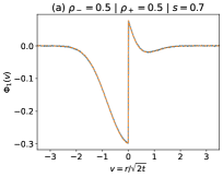
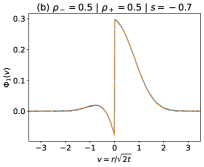
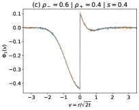
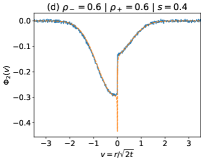
Numerical resolution.— We show in Fig. 2 the profiles at order $1$ and $2$ in $\lambda$ obtained by the numerical resolution of the MFT equations (see SM [39] for details), which are in perfect agreement with results from microscopic Monte Carlo simulations (see SM [39]), for a broad range of parameters. In particular, we consider strong biases, and densities which are far from the extreme low- and high-density limits. Note that the approach can be extended to the paradigmatic case where the initial density of particles is step-like ($\rho=\rho_{+}$ in front of the tracer and $\rho=\rho_{-}$ behind the tracer) [7, 20]. Finally, the plots show that our MFT procedure captures non-trivial dependencies of the correlation profiles on the rescaled distance.

Linear order in $s$.— We first note that, for any bias, at zeroth order in $\lambda$, we retrieve the exact results previously obtained for the mean occupation profiles in the frame of reference of the driven tracer [31, 33]. However, for the next orders ($\Phi_{n}$ with $n\geq 1$), no explicit analytical solution of the MFT problem at arbitrary density is available. We then resort to an expansion in powers of the bias $s$, and define for each order $n$:

$$\Phi_{n}(v)\underset{s\to 0}{=}\Phi_{n}^{(0)}(v)+s\Phi_{n}^{(1)}(v)+s^{2}\Phi_{n}^{(2)}(v)+\dots\>$$ (12)

where $\Phi_{n}^{(0)}$ corresponds to the known symmetric case [8, 9]. At linear order in the bias $s$, we find [39]

$$\Phi_{1}^{(1)}(v)=\frac{1-\rho}{2\rho}\left((2-3\rho)\operatorname{erfc}(v)-(1-\rho)\frac{6}{\pi}\mathrm{e}^{-v^{2}}\right)$$ (13)

$$\Phi_{2}^{(1)}(v)=\frac{(1-\rho)(1-2\rho(1-\rho))}{2\rho^{2}}\operatorname{erfc}(v)+\frac{(1-\rho)^{2}(4-3\rho)}{\pi\rho^{2}}\operatorname{erfc}(v)-\frac{(1-\rho)^{2}}{\rho}\operatorname{erfc}\left(\frac{v}{\sqrt{2}}\right)^{2}\\ -\frac{(1-\rho)^{2}}{2\rho^{2}}G(\sqrt{2}\>v)+\frac{8(1-\rho)^{3}}{\pi^{3/2}\rho^{2}}v\>\mathrm{e}^{-v^{2}}-\frac{4(1-\rho)^{2}(1-2\rho)}{\pi\rho^{2}}\mathrm{e}^{-v^{2}}-\frac{(1-\rho)^{2}}{\pi^{3/2}\rho^{2}}v\>\mathrm{e}^{-\frac{v^{2}}{2}}\>\mathrm{K}_{0}\left(\frac{v^{2}}{2}\right)\>,$$ (14)

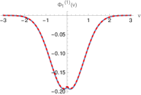
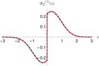
where $G(x)=\frac{1}{\pi}\sqrt{\frac{2}{\pi}}\int_{x}^{\infty}\mathrm{e}^{-z^{2}/4}\mathrm{K}_{0}\left(\frac{z^{2}}{4}\right)\mathrm{d}z$, and $\text{K}_{0}$ is a modified Bessel function of zeroth order. A key point is that, contrary to the first order in $\lambda$, $\Phi_{2}^{(1)}$ is a non-analytic function of the rescaled distance $v$, displaying a logarithmic singularity at the origin. This appears to be a specificity of the driven case, since, in the symmetric case, all $\Phi_{n}$ are analytical functions of the rescaled distance [9]. The functions $\Phi_{1}^{(1)}(v)$ and $\Phi_{2}^{(1)}(v)$ are plotted in Fig. 3 and display perfect agreement with the numerical resolution of the MFT equations. The profile $\Phi_{1}(v)$ measures the correlation between the density at a rescaled distance $v$ from the tracer, and the position of the tracer [8]. When there is no driving force, $\Phi_{1}^{(0)}(v>0)>0$, therefore a fluctuation of $X_{t}$ towards the right is correlated with an increase of the density in front of the tracer, indicating an accumulation of particles in front of the tracer. Here, we find that the linear correction to these correlations due to the presence of the drive, $\Phi_{1}^{(1)}(v)$, is negative, indicating that a positive driving force reduces these correlations, while a negative drive increases them.

Figure 3: Generalised density profiles $\Phi_{n}^{(1)}(v)$ at first order in the bias $s$, at density $\rho=0.6$, obtained from the numerical resolution of the MFT equations (5a) and (5b) (dashed red lined), compared to the analytical expressions (13) and (14) (solid blue). Left: profile $\Phi_{1}^{(1)}$. Right: profile $\Phi_{2}^{(1)}$.

Figure 4: Left: Profile $\Phi_{1}^{(2)}(v)$ at $\rho=0.6$ (18) (solid blue), compared to the numerical resolution of the MFT equations (5a) and (5b) (dashed red). Right: rescaled cumulant $\hat{\kappa}_{2}$ as a function of the bias $s$, obtained from the numerical resolution of the MFT equations (5a) and (5b) (solid blue), compared to the small bias expansion (19) (solid green line). The points are obtained from Monte Carlo simulations (15.8 million simulations, final time 100000). Note that the correction in $s^{2}$ to $\hat{\kappa}_{2}$ is always positive, for all the values of the density $\rho$.

In addition to fully characterize the bath-tracer correlations, the generalized density profiles $\Phi_{n}$ also lead to the cumulants of the tracer’s position. This is made possible by the key relation derived above [Eq. (4)]. We get, for $\hat{\kappa}_{n}\equiv\lim_{t\to\infty}[\kappa_{n}/\sqrt{2t}]$,

$$\hat{\kappa}_{1} = s\frac{1-\rho}{\rho\sqrt{\pi}}+\mathcal{O}(s^{2}),\quad\hat{\kappa}_{2}=\frac{1-\rho}{\rho\sqrt{\pi}}+\mathcal{O}(s^{2}),$$ (15)

$$\hat{\kappa}_{3} = \frac{s}{{\pi^{3/2}\rho^{3}}}\left[(1-\rho)\left(12(1-\rho)^{2}-\pi\left(\left(8-3\sqrt{2}\right)\rho^{2}\right.\right.\right.$$ (16)

$$\left.\left.\left.-3\left(4-\sqrt{2}\right)\rho+3\right)\right)\right]+\mathcal{O}(s^{2})\>.$$

We notice that, up to order $n=3$, $\hat{\kappa}_{n}=s\>\hat{\kappa}_{n+1}^{(s=0)}+\mathcal{O}(s^{2})$, which implies that

$$\psi(\lambda,t)\underset{t\to\infty}{\sim}\psi^{(s=0)}(\lambda,t)+s\>\frac{\mathrm{d}\psi}{\mathrm{d}\lambda}^{(s=0)}+\mathcal{O}(s^{2},\lambda^{4})\>.$$ (17)

On top of that, we checked from the high-density solution obtained in [12, 36] that, when $\rho\to 1$, Eq. (17) holds at any order in $\lambda$, and at arbitrary time. This points towards the generality of this relation.

Beyond linear response.— We next show that explicit analytical results can be obtained beyond linear response which, as we proceed to show, can be quantitatively and even qualitatively significant. In addition, even if our previous expressions provide the leading order in the bias $s$, they do not bring non-trivial information for even cumulants, since the first non-zero correction to the unbiased case is actually of order $s^{2}$ for symmetry reasons. We thus compute the profile $\Phi_{1}$ at quadratic order in the bias, and get [39]

$$\Phi_{1}^{(2)}(v)=\frac{(1-2\rho)(1-\rho)^{2}}{2\rho^{2}}\operatorname{erfc}(v)+\frac{(3-\rho)(1-\rho)^{2}}{\pi\rho^{2}}\operatorname{erfc}(v)-\frac{(1-\rho)^{2}}{2\rho}\text{erfc}\left(\frac{v}{\sqrt{2}}\right)^{2}\\ -\frac{(1-\rho)^{2}}{2\rho^{2}}G(\sqrt{2}\>v)+\frac{5(1-\rho)^{3}}{\pi^{3/2}\rho^{2}}v\>\mathrm{e}^{-v^{2}}-\frac{(3-5\rho)(1-\rho)^{2}}{\pi\rho^{2}}\mathrm{e}^{-v^{2}}-\frac{(1-\rho)^{2}}{\pi^{3/2}\rho^{2}}v\>\mathrm{e}^{-\frac{v^{2}}{2}}\>\mathrm{K}_{0}\left(\frac{v^{2}}{2}\right)\>.$$ (18)

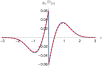
Interestingly, we note that, even at order $1$ in $\lambda$ (and not only at order $2$ as in the linear response analysis discussed above), the density profile is in fact non-analytic at the origin. We stress that this qualitatively different feature emerges beyond linear response.

In addition, the expression of $\Phi_{1}^{(2)}$ yields the $s^{2}$ order of $\hat{\kappa}_{2}=\left.\hat{\kappa}_{2}\right|_{s=0}+s^{2}\>\Delta\hat{\kappa}_{2}^{(2)}+\mathcal{O}(s^{3})$, with

$$\Delta\hat{\kappa}_{2}^{(2)}=\frac{(1-\rho)^{2}(7-5\rho-\pi((\sqrt{2}-3)\rho+2))}{\pi^{3/2}\rho^{3}}\>.$$ (19)

This result constitutes the first determination of the bias-dependence of the variance of a driven tracer in the SEP for an arbitrary density, a problem which has remained open for more than 25 years.

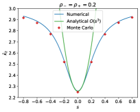
The function $\Phi_{1}^{(2)}(v)$ is plotted in Fig. 3 and displays very good agreement with the results obtained from the numerical procedure described above. We also display the dependence of the second cumulant as a function of the bias for a given value of the density $\rho=0.2$, which shows good agreement with both microscopic Monte Carlo simulations and the numerical resolution as long as the bias is small enough. This cumulant displays an important variation with the bias ($\sim 30\%$), emphasising the quantitative importance of studying the problem beyond linear response (which gives zero variation).

Conclusion.— In this Letter, starting from microscopic considerations, we built a hydrodynamic framework to study both the dynamics of a driven tracer in the SEP and the response of its environment. This allowed us to determine the first cumulants of bath-tracer correlations and of the tracer position at linear order in the bias and at arbitrary density – a regime of parameters that was left aside so far. We also went beyond linear response by determining the second cumulant and the corresponding correlation profile, therefore unveiling for the first time the dependence of the variance of the tracer’s position on the bias. Importantly, this approach is general and can be extended to study other models of single-file transport, by replacing in Eqs. (5a)-(9) the transport coefficients $D$ and $\sigma$ by those of the system under consideration, and adapting the matching condition (10) which can be derived from microscopic considerations, as done here for the SEP.

Acknowledgements.— We thank Alexis Poncet for numerous discussions at early stages of this work, both on analytical and numerical aspects.

References

- Hahn et al. [1996] K. Hahn, J. Kärger, and V. Kukla, Phys. Rev. Lett. 76, 2762 (1996).
- Wei et al. [2000] Q.-H. Wei, C. Bechinger, and P. Leiderer, Science 287, 625 (2000).
- Lin et al. [2005] B. Lin, M. Meron, B. Cui, S. A. Rice, and H. Diamant, Phys. Rev. Lett. 94, 216001 (2005).
- Cambré et al. [2010] S. Cambré, B. Schoeters, S. Luyckx, E. Goovaerts, and W. Wenseleers, Phys. Rev. Lett. 104, 207401 (2010).
- Chou et al. [2011] T. Chou, K. Mallick, and R. K. P. Zia, Rep. Prog. Phys. 74, 116601 (2011).
- Mallick [2015] K. Mallick, Physica A 418, 17 (2015).
- Imamura et al. [2017] T. Imamura, K. Mallick, and T. Sasamoto, Phys. Rev. Lett. 118, 160601 (2017).
- Poncet et al. [2021a] A. Poncet, A. Grabsch, P. Illien, and O. Benichou, Phys. Rev. Lett. 127, 220601 (2021a).
- Grabsch et al. [2021] A. Grabsch, A. Poncet, P. Rizkallah, P. Illien, and O. Bénichou, Science Advances 8, eabm5043 (2021).
- Mallick et al. [2022] K. Mallick, H. Moriya, and T. Sasamoto, Physical Review Letters 129, 40601 (2022).
- Arratia [1983] R. Arratia, The Annals of Probability 11, 362 (1983).
- Illien et al. [2013] P. Illien, O. Bénichou, C. Mejía-Monasterio, G. Oshanin, and R. Voituriez, Physical Review Letters 111, 38102 (2013).
- Hegde et al. [2014] C. Hegde, S. Sabhapandit, and A. Dhar, Phys. Rev. Lett. 113, 120601 (2014).
- Krapivsky et al. [2014] P. L. Krapivsky, K. Mallick, and T. Sadhu, Physical Review Letters 113, 078101 (2014).
- Krapivsky et al. [2015] P. L. Krapivsky, K. Mallick, and T. Sadhu, Journal of Statistical Physics 160, 885 (2015).
- Imamura et al. [2021] T. Imamura, K. Mallick, and T. Sasamoto, Communications in Mathematical Physics 384 (2021).
- Krajenbrink and Le Doussal [2021] A. Krajenbrink and P. Le Doussal, Physical Review Letters 127, 64101 (2021).
- Bettelheim et al. [2022] E. Bettelheim, N. R. Smith, and B. Meerson, Physical Review Letters 128, 130602 (2022).
- Derrida and Gerschenfeld [2009a] B. Derrida and A. Gerschenfeld, Journal of Statistical Physics 137, 978 (2009a).
- Derrida and Gerschenfeld [2009b] B. Derrida and A. Gerschenfeld, Journal of Statistical Physics 136, 1 (2009b).
- Ferrari et al. [1985] P. A. Ferrari, S. Goldstein, and J. L. Lebowitz, Prog. Phys. 10, 405 (1985).
- Habdas et al. [2004] P. Habdas, D. Schaar, A. C. Levitt, and E. R. Weeks, Europhys. Lett. 67, 477 (2004).
- Bausch et al. [1998] A. R. Bausch, F. Ziemann, A. A. Boulbitch, K. Jacobson, and E. Sackmann, Biophys. J. 75, 2038 (1998).
- Leibovich and Barkai [2013] N. Leibovich and E. Barkai, Physical Review E 88, 032107 (2013).
- Lizana et al. [2010] L. Lizana, T. Ambjörnsson, A. Taloni, E. Barkai, and M. A. Lomholt, Physical Review E 81, 051118 (2010).
- Benichou et al. [2018] O. Benichou, P. Illien, G. Oshanin, A. Sarracino, and R. Voituriez, Journal of Physics: Condensed Matter 30, 443001 (2018).
- Leitmann and Franosch [2017] S. Leitmann and T. Franosch, Phys. Rev. Lett. 118, 018001 (2017).
- Leitmann and Franosch [2013] S. Leitmann and T. Franosch, Phys. Rev. Lett. 111, 190603 (2013).
- Cividini et al. [2016a] J. Cividini, A. Kundu, S. N. Majumdar, and D. Mukamel, J Phys. A: Math. Theor. 49, 085002 (2016a).
- Cividini et al. [2016b] J. Cividini, A. Kundu, S. N. Majumdar, and D. Mukamel, J. Stat. Mech. , 053212 (2016b).
- Burlatsky et al. [1996] S. F. Burlatsky, G. Oshanin, M. Moreau, and W. P. Reinhardt, Phys. Rev. E 54, 3165 (1996).
- Burlatsky et al. [1992] S. F. Burlatsky, G. S. Oshanin, A. V. Mogutov, and M. Moreau, Physics Letters A 166, 230 (1992).
- Landim et al. [1998] C. Landim, S. Olla, and S. B. Volchan, Communications in Mathematical Physics 192, 287 (1998).
- Lobaskin and Evans [2020] I. Lobaskin and M. R. Evans, J. Stat. Mech. , 053202 (2020).
- [35] A. Ayyer, arXiv:2001.02425 .
- Poncet et al. [2021b] A. Poncet, O. Benichou, and P. Illien, Physical Review E 103, L040103 (2021b).
- Landim and Volchan [2000] C. Landim and S. Volchan, Stochastic processes and their applications 85, 139 (2000).
- Note [1] The specific situation in [37] corresponds to the case where the driving force imposed on the tracer is compensated by a step of density resulting in a vanishing mean position.
- [39] Supplementary Material, which includes Refs. [48, 49, 50, 51, 52] .
- Note [2] Note that we became aware of an approach similar to the one presented here while we were finalizing this manuscript [53]. Although both works start from the same hydrodynamic equations, the explicit results by Dandekar and Mallick focus on the high-density limit of the problem, while our results are valid at arbitrary density and were out of reach from available microscopic approaches.
- Bertini et al. [2015] L. Bertini, A. De Sole, D. Gabrielli, G. Jona-Lasinio, and C. Landim, Reviews of Modern Physics 87, 593 (2015), arXiv:1404.6466 .
- Spohn [1991] H. Spohn, Large scale dynamics of interacting particles (Springer Berlin, Heidelberg, 1991).
- Evans and Hanney [2005] M. R. Evans and T. Hanney, Journal of Physics A: Mathematical and General 38, R195 (2005).
- Rizkallah et al. [2022] P. Rizkallah, A. Grabsch, P. Illien, and O. Bénichou, arXiv:2207.07549 (2022).
- Kundu and Cividini [2016] A. Kundu and J. Cividini, Europhys. Lett. 115, 54003 (2016), arXiv:1609.05453 .
- Note [3] The methodology presented here is general, but Eqs. (8\@@italiccorr) and (10\@@italiccorr) are written for the SEP.
- Note [4] We give the expressions for , as the ones for can be deduced from the symmetry , and which imposes .
- Poncet [2020] A. Poncet, Dynamique et corrélations de systèmes diffusifs forcés, Ph.D. thesis, Sorbonne Université (2020).
- Bodineau and Derrida [2004] T. Bodineau and B. Derrida, Phys. Rev. Lett. 92, 180601 (2004).
- Evans [2000] M. R. Evans, Braz. J. Phys. 30, 42 (2000).
- Owen [1980] D. B. Owen, Commun. Stat. Simul. Comput. 9, 389 (1980).
- Schulze [2008] T. P. Schulze, J. Comput. Phys 227, 2455 (2008).
- Dandekar and Mallick [2022] R. Dandekar and K. Mallick, arXiv:2207.11242 (2022).