MOTCOM: The Multi-Object Tracking Dataset Complexity Metric
Abstract
There exists no comprehensive metric for describing the complexity of Multi-Object Tracking (MOT) sequences. This lack of metrics decreases explainability, complicates comparison of datasets, and reduces the conversation on tracker performance to a matter of leader board position. As a remedy, we present the novel MOT dataset complexity metric (MOTCOM), which is a combination of three sub-metrics inspired by key problems in MOT: occlusion, erratic motion, and visual similarity. The insights of MOTCOM can open nuanced discussions on tracker performance and may lead to a wider acknowledgement of novel contributions developed for either less known datasets or those aimed at solving sub-problems.
We evaluate MOTCOM on the comprehensive MOT17, MOT20, and MOTSynth datasets and show that MOTCOM is far better at describing the complexity of MOT sequences compared to the conventional density and number of tracks. Project page at https://vap.aau.dk/motcom.
1 Introduction
Tracking has been an important research topic for decades with applications ranging from autonomous driving to fish behavior analysis [41, 26, 13, 34]. The aim is to acquire the full spatio-temporal trajectory of an object of interest, but missing or inaccurate detections can make this a complicated task. When more objects are present in the scene simultaneously it is termed a multi-object tracking (MOT) problem and an additional task is to keep the correct identities of all objects throughout the sequence.
During the previous decade there has been an increase in the development of publicly available MOT datasets [14, 27, 9, 40, 7]. However, there has been no attempt to objectively describe the complexity of a dataset or its sequences except for using simple statistics like density and number of tracks, which are neither adequate nor explanatory, see Figure 1. When a new dataset emerges, the community needs objective metrics to be able to characterize and discuss the dataset with respect to existing datasets, otherwise, ‘gut feeling’ and ‘popularity vote’ will rule.

Furthermore, the absence of an objective MOT sequence complexity metric hinders an informed conversation on the capabilities of trackers developed for different datasets. Nowadays, it is important to rank high on popular MOT benchmark leaderboads in order to gain the attention of the community. This may hinder the acknowledgement of novel solutions that solve sub-problems of MOT particularly well and underrate solutions developed on less popular datasets. We expect that a descriptive and explanatory metric can help remedy these issues.
The literature suggests that there are three main factors that make MOT tasks difficult to solve [3, 31, 1, 2, 26]; namely, occlusion, erratic motion, and visual similarity. We hypothesize that the complexity of MOT sequences can be expressed by a combination of the aforementioned three factors for which we need to construct explicit metrics. Therefore, in this paper we propose the first-ever individual sub-metrics for describing the complexity of the three sub-problems and a unified quantitative MOT dataset complexity metric (MOTCOM) as a combination of these sub-metrics. In Figure 1, we illustrate that MOTCOM is far better at estimating the complexity of the sequences of the recent MOTSynth dataset [12] compared to the commonly used number of tracks and density.
The main contributions of our paper are as follows:
-
1.
The novel metric MOTCOM for describing the complexity of MOT sequences.
-
2.
Three sub-metrics for describing the complexity of MOT sequences with respect to occlusion, erratic motion, and visual similarity.
-
3.
We show that the conventional metrics number of tracks and density are not strong indicators for the complexity of MOT sequences.
-
4.
We evaluate the capability of MOTCOM and demonstrate its superiority against number of tracks and density.
In the next section, we describe and analyse the three sub-problems followed by a presentation of the proposed metrics. In the remainder of the paper, we demonstrate and discuss how the metrics can describe and explain the complexity of MOT sequences.
2 Related Work
The majority of recent trackers utilize the strong performance of deep learning based detectors, e.g., by following the tracking-by-detection paradigm [45, 4, 43], tracking-by-regression [3], through joint training of the detection and tracking steps [33, 49], or as part of an association step [30, 23, 48]. Trackers like Tracktor [3], Chained-Tracker [33], and CenterTrack [49] rely on spatial proximity which makes them vulnerable to sequences with extreme motion and heavy occlusion. At the other end of the spectrum are trackers like QDTrack [30], RetinaTrack [23], and FairMOT [48] which use visual cues for tracking. They are optimized toward tracking visually distinct objects and are not to the same degree limited by erratic motion or vanishing objects but instead sensitive to weak visual features. This indicates that the design of trackers is centered around three core problems: occlusion, erratic motion, and visual similarity. Below, we dive into the literature regarding these problems followed by insights on dataset complexity.
2.0.1 Occlusion.
Occlusions can be difficult to handle and they are often simply treated as missing data [2]. However, in scenes were the objects have weak or similar visual features this can be harmful for the tracking performance [1, 28, 38].
Most authors state that a higher occlusion rate makes tracking harder [6, 22, 25], but they seldom quantify such statements. An exception is the work proposed by Bergmann et al. [3] where they analyzed the tracking results with respect to object visibility, the size of the objects, and missing detections. Moreover, Pedersen et al. [31] argued that the number of objects is less critical than the amount and level of occlusion when it comes to multi-object tracking of fish. They described the complexity of their sequences based on occlusions alone.
2.0.2 Erratic Motion.
Prior information can be used to predict the next state of an object which minimizes the search space and hence reduces the impact of noisy or missing detections. A linear motion model assuming constant velocity is a simple, but effective method for predicting the movement of non-erratic objects like pedestrians [26, 28]. In scenes that include camera motion or complex movement more advanced models may improve tracker performance. Pellegrini et al. [32] proposed incorporating human social behavior into their motion model and Kratz et al. [19] proposed utilizing the movement of a crowd to enhance the tracking of individuals. A downside of many advanced motion models is an often poor ability to generalize to other types of objects or environments.
2.0.3 Visual Similarity.
Visual cues are commonly used in tracklet association and re-identification and are well studied for persons [46], vehicles [18], and animals [37] such as zebrafish [15] and tigers [36]. Modern trackers often solve the association step using CNNs, like Siamese networks, based on a visual affinity model [3, 21, 44, 47]. Such methods rely on visual dissimilarity between the objects. However, tracklet association becomes more difficult when objects are hard to distinguish purely by their appearance.
2.0.4 Dataset Complexity.
Determining the complexity of a dataset is a non-trivial task. One may have a “feeling” or intuition about which datasets are harder than others, but this is subjective and can differ depending on who you ask, as well as differ depending on the task at hand. In order to objectively determine the complexity of a dataset, one has to develop a task-specific framework. An early attempt at this was the suite of 12 complexity measures (c-measures) by Ho and Basu [17], based on concepts such as inter-class overlap and linear separability. However, these c-measures are not suitable for image datasets due to unrealistic assumptions, such as the data being linearly separable. Therefore, Branchaud-Charron et al. [5] developed a complexity measure based on spectral clustering, where the inter-class overlap is quantified through the eigenvalues of an approximated adjacency matrix. This approach was shown to correlate well with the CNN performance on several image datasets. Similarly, Cui et al. [8] presented a framework for evaluating the fine-grainedness of image datasets, by measuring the average distance from data examples to the class centers. Both of these approaches rely on embedding the input images into a feature space by using, e.g., a CNN, and determining the dataset complexity without any indication of what makes the dataset difficult.
In contrast, dataset complexity in the MOT field has so far been determined through simple statistics such as the number of tracks and density. These quantities are currently displayed for every sequence alongside other stats such as resolution and frame rate for the MOTChallenge benchmark datasets [9]. The preliminary works of Bergmann et al. [3] and Pedersen et al. [31] have attempted to further explain what makes a MOT sequence difficult by investigating the effect of occlusions. However, there is no clear way of describing the complexity of MOT sequences and the current methods have not been verified.
3 Challenges in Multi-Object Tracking
MOT covers the task of obtaining the spatio-temporal trajectories of multiple objects in a sequence of consecutive frames. Depending on the specific task, the objects may be represented as 3D points [31], pixel-level segmentation masks [42], or bounding boxes [29]. Despite the different representation forms, the concepts of occlusion, erratic motion, and visual similarity apply to all of them and add to the complexity of the sequences.
3.0.1 Occlusion.
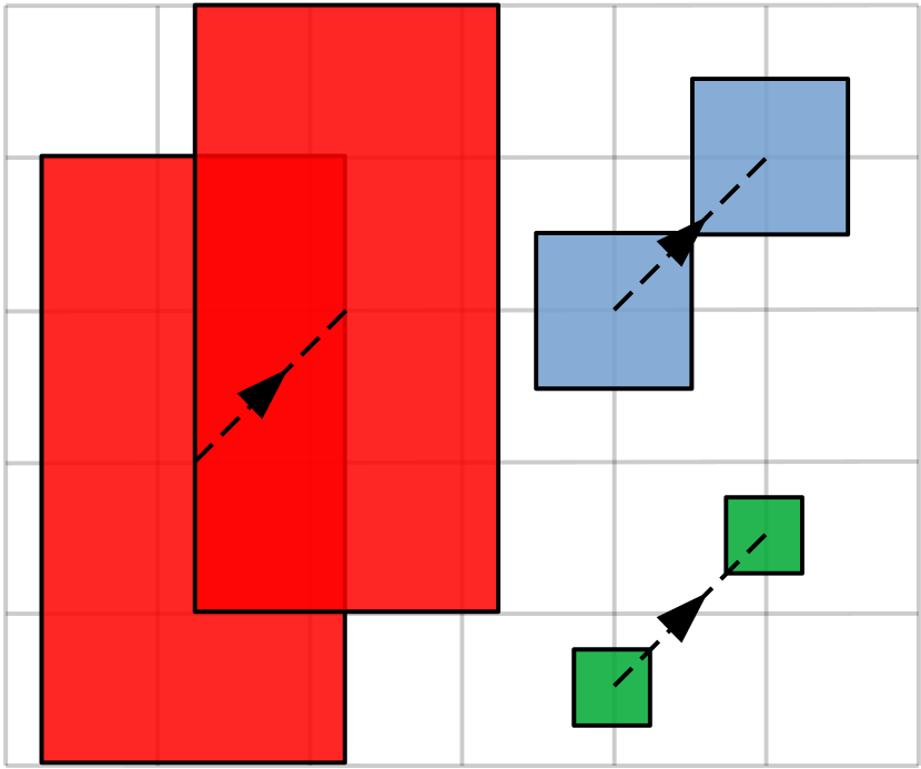
Occlusion describes situations where the visual information of an object within the camera view is partially or fully hidden. There are three types of occlusion: self-occlusion, scene-occlusion, and inter-object-occlusion [1]. Self-occlusion can reduce the visibility of parts of an object, e.g., if a hand is placed in front of a face, but defining the level of self-occlusion is non-trivial and depends on the type of object. Scene-occlusion occurs when a static object is located in the line of sight between the camera and the target object, thereby decreasing the visual information of the target. A scene-occlusion is marked by the red box in Figure 2(a), where flowers partially occlude a sitting person.
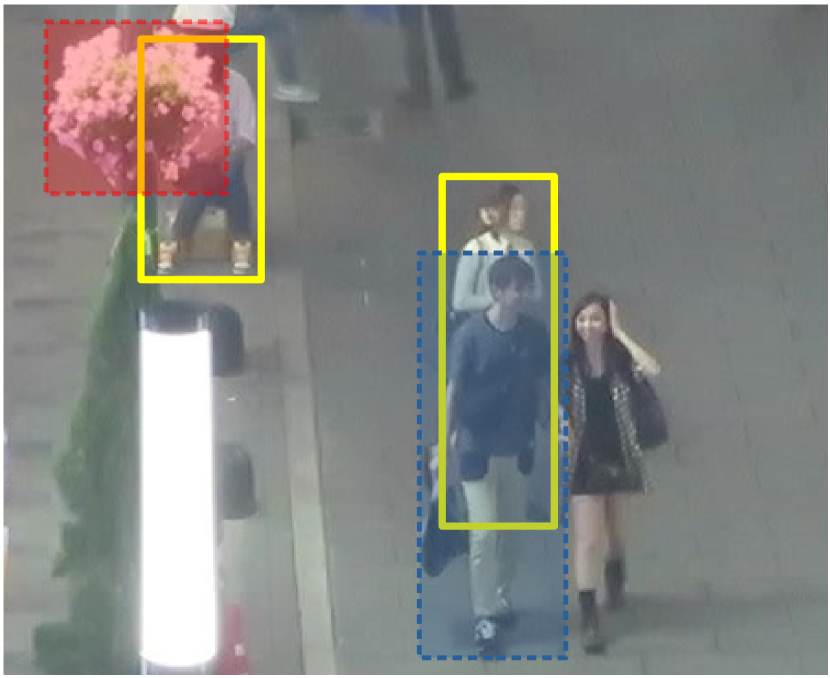
Inter-object-occlusion is typically the most difficult to handle, especially if the objects are of the same type, as the trajectories of multiple objects cross. An example can be seen in Figure 2(a), where the blue box marks a person that partially occludes another person.
3.0.2 Erratic Motion.
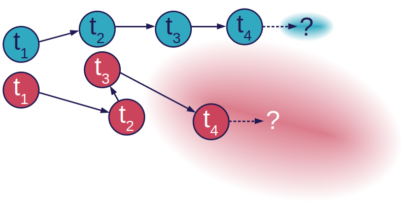
We use motion as a term for an object’s spatial displacement between frames. This is typically caused by the locomotive behavior of the object itself, camera motion, or a combination. As the number of factors that influence the observed motion increases, the motion becomes harder to predict. An example of two objects exhibiting different types of motion is presented in Figure 2(b). The blue object moves with approximately the same direction and speed between the time steps. Predicting the next state of the object seems trivial and the search space is correspondingly small. On the other hand, the red object behaves erratically and unpredictably while the motion model is less confident as illustrated by the larger search space.
3.0.3 Visual Similarity.
The visual appearance of objects can vary widely depending on the type of object and type of scene. Appearance is especially important when tracking is lost, for example, due to occlusion, and re-identification is a common tool for associating broken tracklets. The complexity of this process depends on the visual similarity between objects, but intra-object similarity also plays a role. As an object moves through a scene, its appearance can change from the perspective of the viewer. The object may turn around, increase its distance to the camera, or the illumination conditions may change. Aside from the visual cues, the object’s position is also critical. Intuitively, it becomes less likely to confuse objects as the spatial distance between them increases.
4 The MOTCOM Metrics
We propose individual metrics to describe the level of occlusion, erratic motion, and visual similarity for MOT sequences. Subsequently, we combine these three sub-metrics into a higher-level metric that describes the overall complexity of the sequences.
4.0.1 Preliminaries
We define a MOT sequence as a set of frames containing a set of objects . The objects do not have to be present in every frame, therefore, we define the set of frames where a given object is present by . The objects present in a given frame are defined as the set . At each frame an object is represented by its center-position in image coordinates and the height and width of the surrounding bounding box .
4.1 Occlusion Metric
As mentioned in Section 3, occlusion can be divided into three types: self-, scene- and inter-object occlusion. In order to quantify the occlusion rate in a sequence, one should ideally account for all three types. However, it is most often non-trivial to determine the level of self-occlusion and it is commonly not taken into account in MOT. Pedersen et al. [31] used the ratio of intersecting object bounding boxes to determine the inter-object occlusion rate. Similarly, the MOT16, MOT17, and MOT20 datasets include a visibility score based on the intersection over area (IoA) of both inter- and scene-objects [9], where IoA is formulated as the area of intersection over the area of the target.
Following this trend, we omit self-occlusion and base the occlusion metric, OCOM, on the IoA and compute it as
| (1) |
where is the mean level of occlusion of object . is in the interval where 0 is fully visible and 1 is fully occluded. It is assumed that terrestrial objects move on a ground plane which allows us to interpret their y-values as pseudo-depth and decide on the ordering. Annotations are needed to calculate the occlusion level for objects moving in 3D. OCOM is defined in the interval where a higher value means more occlusion and a harder problem to solve.
4.2 Motion Metric
The proposed motion metric, MCOM, is based on the assumption that objects move linearly when observed at small time steps. If this assumption is not upheld, it is a sign of erratic motion and thereby a more complex MOT sequence.
Initially, the displacement vector, , between the object’s position in the current and past time step is calculated as
| (2) |
where is the position of object at time , defined by its - and -coordinates, and describes the temporal step size. When calculating the displacement between two consecutive frames . The displacement vector in the first frame of a trajectory is set to zero and is capped by the first and last frame of a trajectory when the object is not present at time .
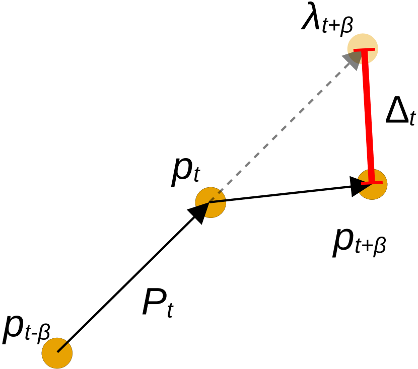
The position in the next time step is predicted using a linear motion model with constant velocity based on the current position and the calculated displacement vector. The position is predicted by
| (3) |
The error between the predicted and true position of the object is calculated by
| (4) |
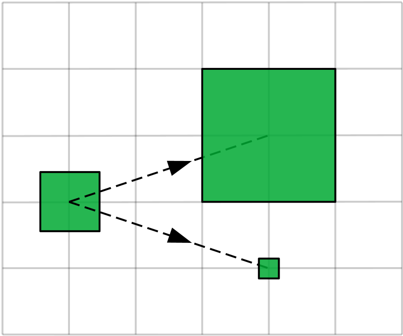
where is the Euclidean distance function and a larger indicates a more complex motion. See Figure 3(a) for an illustration of how the displacement error is calculated. This approach may seem overly simplified, but it encapsulates changes in both direction and velocity. Furthermore, it is deliberately sensitive to low frame rates and camera motion, as both factors add to the complexity of tracking sequences.
Inspired by the analysis of decreasing tracking performance with respect to smaller object sizes by Bergmann et al. [3], the size is also taken into consideration. The combination of size and movement affects the difficulty of predicting the next state of the object. In Figure 3(b), the rectangles are equally displaced but do not experience the same displacement relative to their size. Intuitively, if a set of objects are moving at similar speeds, it is harder to track the smaller objects due to their lower spatio-temporal overlap.
Accordingly, the motion-based complexity measure is based on the displacement relative to the size of the object. As illustrated in Figure 3(c), the size of the object may change between two time steps. The direction of the change is critical as the displacement is less distinct if the size of the object is increasing, compared to the opposite situation. Therefore, we multiply the current size of the object with the change in object size to get the transformed object size
| (5) |
where and and are the height and width of object at time step , respectively. The motion complexity measure is then calculated as the mean size-compensated displacement across all frames, , and all objects at each frame, , and weighted by the log-sigmoid function
| (6) |
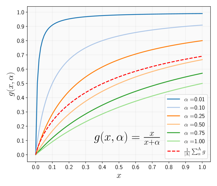
where the average of is used to avoid manually deciding on a specific value for . The use of the function is motivated by the aim of having an output in the range , where a higher number describes a more complex motion. The function is given by
| (7) |
where affects the gradient of the monotonically increasing function and indicates the point where the output of the function will reach 0.5 as illustrated in Figure 4. The function is designed such that displacements in the lower ranges are weighted higher. The argument for this choice is based on the assumption that minor increments to an extraordinarily erratic locomotive behavior have less impact on the complexity.
4.3 Visual Similarity Metric
In order to define a metric that links an object’s visual appearance with tracking complexity, we investigate how similar an object in one frame is compared to itself and other objects in the next frame. Two objects may look similar, but they cannot occupy the same spatial position. Therefore, we propose a spatial-aware visual similarity metric called VCOM.
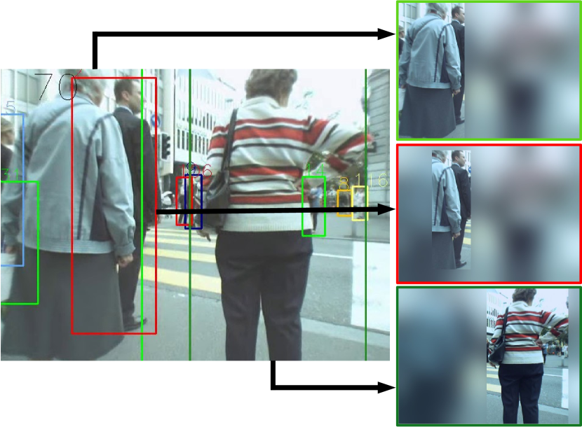
VCOM consists of a preprocessing, feature extraction, and distance evaluation step. For every object in every frame an image is produced with the object’s bounding box in focus and a heavy blurred background. We blur the image using a discrete Gaussian function, except in the region of the object’s bounding box as visualized in Figure 5(a).
A feature embedding is then extracted from each of the preprocessed images. As opposed to looking at the bounding box alone, using the entire image allows us to retain and embed spatial information in the feature vector. The object’s location is especially valuable in scenes with similarly looking objects and the blurred background contributes with low frequency information of the surroundings.
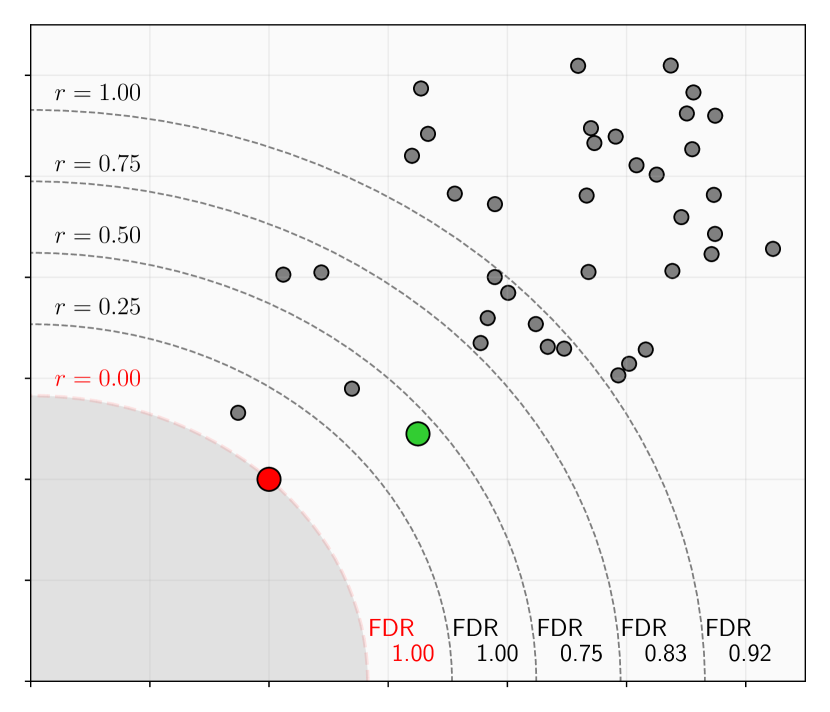
We blur the image with a Gaussian kernel with a fixed size of 201 and a sigma of 38 and extract the image features using an ImageNet [10] pre-trained ResNet-18 [16] model. We measure the similarity between the feature vector of the target object in frame and the feature vectors of all the objects in frame by computing the Euclidean distance. The uncertainty increases if more objects are located within the proximity of the target. Therefore, we do not only look for the nearest neighbor, but rather the number of objects within a given distance, , from the target feature vector
| (8) |
where is the distance to the nearest neighbor and is a distance ratio. The ratio is multiplied by the distance to the nearest neighbor in order to account for the variance in scale, e.g., as induced by object resolution or distinctiveness.
An object within the distance boundary that shares the same identity as the target object is considered a true positive (TP) and all other objects are considered false positives (FP). By measuring the complexity based on the false discovery rate, , we get an output in the range where a higher number indicates a more complex task. An illustrative example of how the FDR is determined based on the distance ratio can be seen in Figure 5(b). It is ambiguous to choose a single optimal distance ratio . Therefore, we calculate VCOM based on the average of distance ratios from the set
| (9) |
4.4 MOTCOM
Occlusion alone does not necessarily indicate an overwhelming problem if the object follows a known motion model or if it is visually distinct. The same is true for erratic motion and visual similarity when viewed in isolation. However, the combination of occlusion, erratic motion, and visual similarity becomes increasingly difficult to handle.
Therefore, we combine the occlusion, erratic motion, and visual similarity metrics into a single MOTCOM metric that describes the overall complexity of a sequence. MOTCOM is computed as the weighted arithmetic mean of the three sub-metrics and is given by
| (10) |
where , , and are the weights for the three sub-metrics. Equal weighting can be obtained by setting , while custom weights may be suitable for specific applications. During evaluation we weight the sub-metrics equally as we deem each of the sub-problems equally difficult to handle.
5 Evaluation
In the following experimental section, we demonstrate that MOTCOM is able to describe the complexity of MOT sequences and is superior to density and number of tracks. In order to do this, we compare the estimated complexity levels with ground truth representations. Such ground truths are not readily available, but a strong proxy can be obtained by ranking the sequences based on the performance of state-of-the-art trackers [20]. There exist many performance metrics with two of the most popular being MOTA [39] and IDF1 [35]. However, we apply the recent HOTA metric [24], which was proposed in response to the imbalance between detection, association, and localization within traditional metrics. Additionally, HOTA is the tracker performance metric that correlates the strongest with MOT complexity based on human assessment [24]. In the remainder of this section, we present the datasets and evaluation metrics we use to experimentally verify the applicability of MOTCOM.




5.1 Ground Truth
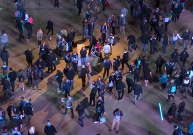
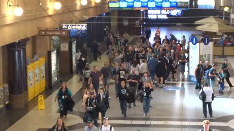
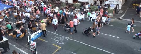
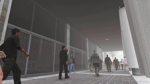
In order to create a strong foundation for the evaluation, we are in need of benchmark datasets with consistent annotation standards and leader boards with a wide range of state-of-the-art trackers. Therefore, we evaluate MOTCOM on the popular MOT17 [27] and MOT20 [9] datasets111With permission from the MOTChallenge benchmark authors.. There are seven sequences in the test split of MOT17 and four sequences in the test split of MOT20, some of which are presented in Figure 6. Furthermore, leader boards are provided for both benchmarks with results from 212 trackers for MOT17 and 80 trackers for MOT20. We use the results from the top-30 ranked trackers222Leader board results obtained on March 4, 2022. based on the average HOTA score, so as to limit unstable and fluctuating performances.
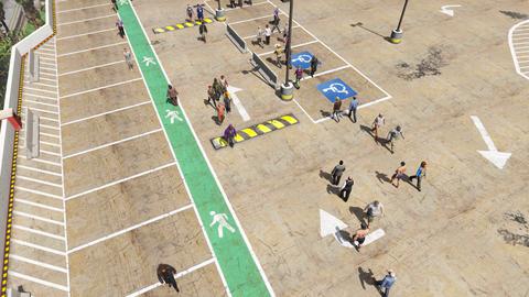
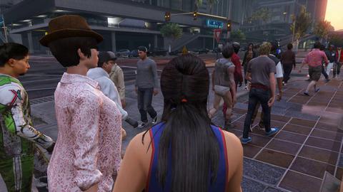
In order to strengthen and support the evaluation, we include the training split of the fully synthetic MOTSynth dataset [12] which contains 764 varied sequences of pedestrians. A few samples from the dataset can be seen in Figure 7. In order to obtain ground truth tracker performance for MOTSynth, we train and test a CenterTrack model [49] on the data. We have chosen CenterTrack as it has been shown to perform well when trained on synthetic data [12].
5.2 Evaluation Metrics
We evaluate and compare the dataset complexity metrics by their ability to rank the MOT sequences according to the HOTA score of the trackers. We rank the sequences from simple to complex by their density, number of tracks (abbr. tracks), MOTCOM score, and HOTA score. Depending on the metric, the ranking is in decreasing (HOTA) or increasing order (density, tracks, MOTCOM). The absolute difference between the ranks, known as Spearman’s Footrule Distance (FD) [11], gives the distance between the ground truth and estimated ranks
| (11) |
where is the number of sequences and is density, tracks, or MOTCOM. In order to directly compare results of sets of different lengths, we normalize the FD by the maximal possible distance which is computed as
| (12) |
Finally, we compute the normalized FD, .
6 Results
In Table 1, we present the mean FD of the ranks of density, tracks, and MOTCOM against the ground truth ranks dictated by the average top-30 HOTA performance on the MOT17 and MOT20 test splits (individually and in combination). The numbers in parentheses are the normalized FD. Generally, MOTCOM has a considerably lower FD compared to density and tracks. This suggests that MOTCOM is better at ranking the sequences according to the HOTA performance
| Top-30 | MOT17test | MOT20test | Combined | |||
|---|---|---|---|---|---|---|
| Density | 1.71 (0.50) | 1.00 (0.50) | 3.82 (0.70) | |||
| Tracks | 2.57 (0.75) | 1.50 (0.75) | 3.82 (0.70) | |||
| MOTCOM | 0.86 (0.25) | 0.00 (0.00) | 1.45 (0.27) |
| CenterTrack | MOTChltest | MOTChltrain | MOTChlboth | MOTSynth | ||||
|---|---|---|---|---|---|---|---|---|
| Density | 3.27 (0.60) | 4.18 (0.77) | 7.36 (0.67) | 238.71 (0.63) | ||||
| Tracks | 2.73 (0.50) | 3.64 (0.67) | 6.64 (0.60) | 193.50 (0.51) | ||||
| MOTCOM | 2.36 (0.43) | 2.18 (0.40) | 4.82 (0.44) | 100.17 (0.26) |
A similar tendency can be seen for the CenterTrack-based results presented in Table 2. In order to increase the number of samples, we have evaluated CenterTrack on both the train and test splits of the MOT17 and MOT20 datasets. MOTChltest and MOTChltrain are the test and train sequences, respectively, of MOT17 and MOT20. MOTChlboth includes all the sequences from MOT17 and MOT20. These results support our claim that MOTCOM is better at estimating the complexity of MOT sequences compared to density and tracks.
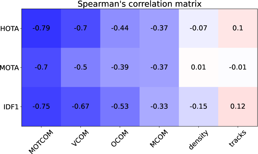
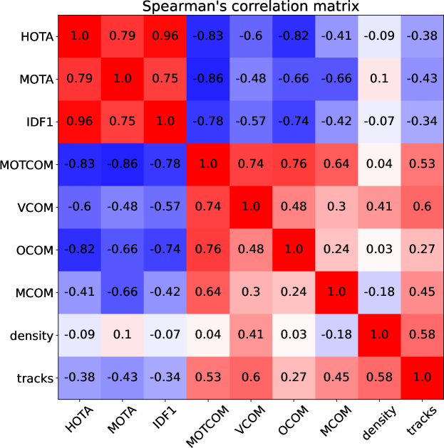
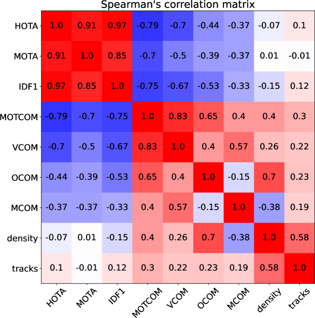
We present a Spearman’s correlation matrix in Figure 8 based on the top-30 trackers evaluated for the combined MOT17 and MOT20 test splits. It indicates that the density and tracks do not correlate with HOTA, MOTA, or IDF1, whereas MOTCOM has a strong negative correlation with all the performance metrics. Trackers evaluated on sequences with high MOTCOM scores tend to have lower performance while sequences with low MOTCOM scores gives higher performance. This underlines that MOTCOM can indeed be used to understand the complexity of MOT sequences.
7 Discussion
Our complexity metric MOTCOM provides tracker researchers and dataset developers a comprehensive score to investigate and describe the complexity of MOT sequences without the need for multiple baseline evaluations of different tracking methods. This allows for an objective comparison of different datasets without introducing potential training bias. Currently, the assessment of tracker performance is roughly speaking reduced to a placement on a benchmark leader board. This underrates novel solutions developed for less popular datasets or methods designed explicitly to solve sub-tasks such as occlusion or erratic motion.
Supplemented by the sub-metrics, MOTCOM provides a deeper understanding and more informed discussions on dataset composition and tracker performance, which will increase the explanability of MOT. In order to illustrate this, we discuss the performance of CenterTrack on the MOTSynth dataset with respect to MOTCOM. Here we see that the occlusion level (OCOM) in Figure 9 has a strong negative correlation with the HOTA score and the visual similarity metric (VCOM) has a relatively weak correlation with HOTA. Both cases expose the design of CenterTrack, which does not contain a module to handle lost tracks and is not dependent on visual cues for tracking. For the motion metric (MCOM) we see two distributions; one in the lower end and one in the upper end of the MCOM range. The objects are expected to behave similarly, so this indicates that parts of the MOTSynth sequences include heavy camera motion which is difficult for CenterTrack to handle. In Figure 10, we show that MOTCOM is far better at estimating the complexity level compared to tracks and density.


8 Conclusion
We propose MOTCOM, the first meaningful and descriptive MOT dataset complexity metric, and show that it is preferable for describing the complexity of MOT sequences compared to the conventional methods of number of tracks and density. MOTCOM is a combination of three individual sub-metrics that describe the complexity of MOT sequences with respect to key obstacles in MOT: occlusion, erratic motion, and visual similarity. The information provided by MOTCOM can assist tracking researchers and dataset developers in acquiring a deeper understanding of MOT sequences and trackers. We strongly suggest that the community uses MOTCOM as the prevalent complexity measure for increasing the explainability of MOT trackers and datasets.
Acknowledgements
This work has been funded by the Independent Research Fund Denmark under case number 9131-00128B.
References
- [1] Andriyenko, A., Roth, S., Schindler, K.: An analytical formulation of global occlusion reasoning for multi-target tracking. In: 2011 IEEE International Conference on Computer Vision Workshops (ICCV Workshops). pp. 1839–1846. IEEE (2011). https://doi.org/10.1109/ICCVW.2011.6130472
- [2] Andriyenko, A., Schindler, K.: Multi-target tracking by continuous energy minimization. In: 2011 IEEE Conference on Computer Vision and Pattern Recognition (CVPR). pp. 1265–1272 (2011). https://doi.org/10.1109/CVPR.2011.5995311
- [3] Bergmann, P., Meinhardt, T., Leal-Taixé, L.: Tracking without bells and whistles. In: 2019 IEEE/CVF International Conference on Computer Vision (ICCV). pp. 941–951 (2019). https://doi.org/10.1109/ICCV.2019.00103
- [4] Bewley, A., Ge, Z., Ott, L., Ramos, F., Upcroft, B.: Simple online and realtime tracking. In: 2016 IEEE International Conference on Image Processing (ICIP). pp. 3464–3468 (2016). https://doi.org/10.1109/ICIP.2016.7533003
- [5] Branchaud-Charron, F., Achkar, A., Jodoin, P.M.: Spectral metric for dataset complexity assessment. In: 2019 IEEE/CVF Conference on Computer Vision and Pattern Recognition (CVPR). pp. 3210–3219 (2019). https://doi.org/10.1109/CVPR.2019.00333
- [6] Cao, X., Guo, S., Lin, J., Zhang, W., Liao, M.: Online tracking of ants based on deep association metrics: method, dataset and evaluation. Pattern Recognition 103 (2020). https://doi.org/10.1016/j.patcog.2020.107233
- [7] Chang, M.F., Lambert, J., Sangkloy, P., Singh, J., Bak, S., Hartnett, A., Wang, D., Carr, P., Lucey, S., Ramanan, D., Hays, J.: Argoverse: 3d tracking and forecasting with rich maps. In: 2019 IEEE/CVF Conference on Computer Vision and Pattern Recognition (CVPR). pp. 8740–8749 (2019). https://doi.org/10.1109/CVPR.2019.00895
- [8] Cui, Y., Gu, Z., Mahajan, D., van der Maaten, L., Belongie, S., Lim, S.N.: Measuring dataset granularity (2019). https://doi.org/10.48550/ARXIV.1912.10154
- [9] Dendorfer, P., Osep, A., Milan, A., Schindler, K., Cremers, D., Reid, I., Roth, S., Leal-Taixé, L.: Motchallenge: A benchmark for single-camera multiple target tracking. International Journal of Computer Vision (IJCV) 129, 845–881 (2021). https://doi.org/10.1007/s11263-020-01393-0
- [10] Deng, J., Dong, W., Socher, R., Li, L.J., Kai Li, Li Fei-Fei: Imagenet: A large-scale hierarchical image database. In: 2009 IEEE Conference on Computer Vision and Pattern Recognition (CVPR). pp. 248–255 (2009). https://doi.org/10.1109/CVPR.2009.5206848
- [11] Diaconis, P., Graham, R.L.: Spearman’s footrule as a measure of disarray. Journal of the Royal Statistical Society: Series B (Methodological) 39(2), 262–268 (1977). https://doi.org/10.1111/j.2517-6161.1977.tb01624.x
- [12] Fabbri, M., Brasó, G., Maugeri, G., Cetintas, O., Gasparini, R., Ošep, A., Calderara, S., Leal-Taixe, L., Cucchiara, R.: Motsynth: How can synthetic data help pedestrian detection and tracking? In: 2021 IEEE/CVF International Conference on Computer Vision (ICCV). pp. 10829–10839 (2021). https://doi.org/10.1109/ICCV48922.2021.01067
- [13] Gade, R., Moeslund, T.B.: Constrained multi-target tracking for team sports activities. IPSJ Transactions on Computer Vision and Applications 10, 2 (2018). https://doi.org/10.1186/s41074-017-0038-z
- [14] Geiger, A., Lenz, P., Urtasun, R.: Are we ready for autonomous driving? the kitti vision benchmark suite. In: 2012 IEEE Conference on Computer Vision and Pattern Recognition (CVPR). pp. 3354–3361 (2012). https://doi.org/10.1109/CVPR.2012.6248074
- [15] Haurum, J.B., Karpova, A., Pedersen, M., Bengtson, S.H., Moeslund, T.B.: Re-identification of zebrafish using metric learning. In: 2020 IEEE Winter Applications of Computer Vision Workshops (WACVW). pp. 1–11 (2020). https://doi.org/10.1109/WACVW50321.2020.9096922
- [16] He, K., Zhang, X., Ren, S., Sun, J.: Deep residual learning for image recognition. In: 2016 IEEE Conference on Computer Vision and Pattern Recognition (CVPR). pp. 770–778 (2016). https://doi.org/10.1109/CVPR.2016.90
- [17] Ho, T.K., Basu, M.: Complexity measures of supervised classification problems. IEEE Transactions on Pattern Analysis and Machine Intelligence (PAMI) 24(3), 289–300 (2002). https://doi.org/10.1109/34.990132
- [18] Khan, S.D., Ullah, H.: A survey of advances in vision-based vehicle re-identification. Computer Vision and Image Understanding 182, 50–63 (2019). https://doi.org/10.1016/j.cviu.2019.03.001
- [19] Kratz, L., Nishino, K.: Tracking with local spatio-temporal motion patterns in extremely crowded scenes. In: 2010 IEEE Computer Society Conference on Computer Vision and Pattern Recognition (CVPR). pp. 693–700 (2010). https://doi.org/10.1109/CVPR.2010.5540149
- [20] Leal-Taixé, L., Milan, A., Schindler, K., Cremers, D., Reid, I., Roth, S.: Tracking the trackers: an analysis of the state of the art in multiple object tracking. arXiv (2017). https://doi.org/10.48550/ARXIV.1704.02781
- [21] Leal-Taixé, L., Canton-Ferrer, C., Schindler, K.: Learning by tracking: Siamese cnn for robust target association. In: 2016 IEEE Conference on Computer Vision and Pattern Recognition Workshops (CVPRW). pp. 418–425 (2016). https://doi.org/10.1109/CVPRW.2016.59
- [22] Liu, C., Yao, R., Rezatofighi, S.H., Reid, I., Shi, Q.: Model-free tracker for multiple objects using joint appearance and motion inference. IEEE Transactions on Image Processing 29, 277–288 (2020). https://doi.org/10.1109/TIP.2019.2928123
- [23] Lu, Z., Rathod, V., Votel, R., Huang, J.: Retinatrack: Online single stage joint detection and tracking. In: 2020 IEEE/CVF Conference on Computer Vision and Pattern Recognition (CVPR). pp. 14656–14666 (2020). https://doi.org/10.1109/CVPR42600.2020.01468
- [24] Luiten, J., Osep, A., Dendorfer, P., Torr, P., Geiger, A., Leal-Taixé, L., Leibe, B.: Hota: A higher order metric for evaluating multi-object tracking. International Journal of Computer Vision (IJCV) p. 548–578 (2021). https://doi.org/10.1007/s11263-020-01375-2
- [25] Luo, W., Kim, T.K., Stenger, B., Zhao, X., Cipolla, R.: Bi-label propagation for generic multiple object tracking. In: 2014 IEEE Conference on Computer Vision and Pattern Recognition (CVPR). pp. 1290–1297 (2014). https://doi.org/10.1109/CVPR.2014.168
- [26] Luo, W., Xing, J., Milan, A., Zhang, X., Liu, W., Kim, T.K.: Multiple object tracking: A literature review. Artificial Intelligence 293, 103448 (2021). https://doi.org/10.1016/j.artint.2020.103448
- [27] Milan, A., Leal-Taixé, L., Reid, I., Roth, S., Schindler, K.: Mot16: A benchmark for multi-object tracking. arXiv (2016). https://doi.org/10.48550/ARXIV.1603.00831
- [28] Milan, A., Roth, S., Schindler, K.: Continuous energy minimization for multitarget tracking. IEEE Transactions on Pattern Analysis and Machine Intelligence (PAMI) 36(1), 58–72 (2014). https://doi.org/10.1109/TPAMI.2013.103
- [29] Milan, A., Schindler, K., Roth, S.: Challenges of ground truth evaluation of multi-target tracking. In: 2013 IEEE Conference on Computer Vision and Pattern Recognition Workshops (CVPRW). pp. 735–742 (2013). https://doi.org/10.1109/CVPRW.2013.111
- [30] Pang, J., Qiu, L., Li, X., Chen, H., Li, Q., Darrell, T., Yu, F.: Quasi-dense similarity learning for multiple object tracking. In: 2021 IEEE/CVF Conference on Computer Vision and Pattern Recognition (CVPR). pp. 164–173 (2021). https://doi.org/10.1109/CVPR46437.2021.00023
- [31] Pedersen, M., Haurum, J.B., Hein Bengtson, S., Moeslund, T.B.: 3d-zef: A 3d zebrafish tracking benchmark dataset. In: 2020 IEEE/CVF Conference on Computer Vision and Pattern Recognition (CVPR). pp. 2423–2433 (2020). https://doi.org/10.1109/CVPR42600.2020.00250
- [32] Pellegrini, S., Ess, A., Schindler, K., van Gool, L.: You’ll never walk alone: Modeling social behavior for multi-target tracking. In: 2009 IEEE 12th International Conference on Computer Vision (ICCV). pp. 261–268 (2009). https://doi.org/10.1109/ICCV.2009.5459260
- [33] Peng, J., Wang, C., Wan, F., Wu, Y., Wang, Y., Tai, Y., Wang, C., Li, J., Huang, F., Fu, Y.: Chained-tracker: Chaining paired attentive regression results for end-to-end joint multiple-object detection and tracking. In: Vedaldi, A., Bischof, H., Brox, T., Frahm, J.M. (eds.) Computer Vision – ECCV 2020. pp. 145–161. Springer, Cham (2020). https://doi.org/10.1007/978-3-030-58548-8_9
- [34] Pérez-Escudero, A., Vicente-Page, J., Hinz, R.C., Arganda, S., De Polavieja, G.G.: idtracker: tracking individuals in a group by automatic identification of unmarked animals. Nature methods 11(7), 743–748 (2014). https://doi.org/10.1038/nmeth.2994
- [35] Ristani, E., Solera, F., Zou, R., Cucchiara, R., Tomasi, C.: Performance measures and a data set for multi-target, multi-camera tracking. In: Hua, G., Jégou, H. (eds.) Computer Vision – ECCV 2016 Workshops, pp. 17–35. Springer, Cham (2016). https://doi.org/10.1007/978-3-319-48881-3_2
- [36] Schneider, S., Taylor, G.W., Kremer, S.C.: Similarity learning networks for animal individual re-identification - beyond the capabilities of a human observer. In: 2020 IEEE Winter Applications of Computer Vision Workshops (WACVW). pp. 44–52 (2020). https://doi.org/10.1109/WACVW50321.2020.9096925
- [37] Schneider, S., Taylor, G.W., Linquist, S., Kremer, S.C.: Past, present and future approaches using computer vision for animal re-identification from camera trap data. Methods in Ecology and Evolution 10(4), 461–470 (2019). https://doi.org/10.1111/2041-210X.13133
- [38] Stadler, D., Beyerer, J.: Improving multiple pedestrian tracking by track management and occlusion handling. In: 2021 IEEE/CVF Conference on Computer Vision and Pattern Recognition (CVPR). pp. 10953–10962 (2021). https://doi.org/10.1109/CVPR46437.2021.01081
- [39] Stiefelhagen, R., Bernardin, K., Bowers, R., Garofolo, J., Mostefa, D., Soundararajan, P.: The clear 2006 evaluation. In: Stiefelhagen, R., Garofolo, J. (eds.) Multimodal Technologies for Perception of Humans. pp. 1–44. Springer, Berlin, Heidelberg (2007). https://doi.org/10.1007/978-3-540-69568-4_1
- [40] Sun, P., Kretzschmar, H., Dotiwalla, X., Chouard, A., Patnaik, V., Tsui, P., Guo, J., Zhou, Y., Chai, Y., Caine, B., Vasudevan, V., Han, W., Ngiam, J., Zhao, H., Timofeev, A., Ettinger, S., Krivokon, M., Gao, A., Joshi, A., Zhang, Y., Shlens, J., Chen, Z., Anguelov, D.: Scalability in perception for autonomous driving: Waymo open dataset. In: 2020 IEEE/CVF Conference on Computer Vision and Pattern Recognition (CVPR). pp. 2443–2451 (2020). https://doi.org/10.1109/CVPR42600.2020.00252
- [41] Uhlmann, J.K.: Algorithms for multiple-target tracking. American Scientist 80(2), 128–141 (1992)
- [42] Voigtlaender, P., Krause, M., Osep, A., Luiten, J., Sekar, B.B.G., Geiger, A., Leibe, B.: Mots: Multi-object tracking and segmentation. In: 2019 IEEE/CVF Conference on Computer Vision and Pattern Recognition (CVPR). pp. 7934–7943 (2019). https://doi.org/10.1109/CVPR.2019.00813
- [43] Wojke, N., Bewley, A., Paulus, D.: Simple online and realtime tracking with a deep association metric. In: 2017 IEEE International Conference on Image Processing (ICIP). pp. 3645–3649 (2017). https://doi.org/10.1109/ICIP.2017.8296962
- [44] Xiang, Y., Alahi, A., Savarese, S.: Learning to track: Online multi-object tracking by decision making. In: 2015 IEEE International Conference on Computer Vision (ICCV). pp. 4705–4713 (2015). https://doi.org/10.1109/ICCV.2015.534
- [45] Xu, J., Cao, Y., Zhang, Z., Hu, H.: Spatial-temporal relation networks for multi-object tracking. In: 2019 IEEE/CVF International Conference on Computer Vision (ICCV). pp. 3987–3997 (2019). https://doi.org/10.1109/ICCV.2019.00409
- [46] Ye, M., Shen, J., Lin, G., Xiang, T., Shao, L., Hoi, S.C.H.: Deep learning for person re-identification: A survey and outlook. IEEE Transactions on Pattern Analysis and Machine Intelligence (PAMI) 44(6), 2872–2893 (2022). https://doi.org/10.1109/TPAMI.2021.3054775
- [47] Yin, J., Wang, W., Meng, Q., Yang, R., Shen, J.: A unified object motion and affinity model for online multi-object tracking. In: 2020 IEEE/CVF Conference on Computer Vision and Pattern Recognition (CVPR). pp. 6767–6776 (2020). https://doi.org/10.1109/CVPR42600.2020.00680
- [48] Zhang, Y., Wang, C., Wang, X., Zeng, W., Liu, W.: Fairmot: On the fairness of detection and re-identification in multiple object tracking. International Journal of Computer Vision (IJCV) 129(11), 3069–3087 (2021). https://doi.org/10.1007/s11263-021-01513-4
- [49] Zhou, X., Koltun, V., Krähenbühl, P.: Tracking objects as points. In: Vedaldi, A., Bischof, H., Brox, T., Frahm, J.M. (eds.) Computer Vision – ECCV 2020. pp. 474–490. Springer, Cham (2020). https://doi.org/10.1007/978-3-030-58548-8_28
Supplementary Materials
0..0.1 Computing MOTCOM.
We have evaluated four averaging methods for combining the sub-metrics into MOTCOM. The four methods are the arithmetic, quadratic, geometric, and harmonic means and they are presented in Equation (13), Equation (14),Equation (15), and Equation (16), respectively.
| (13) | (14) |
| (15) | (16) |
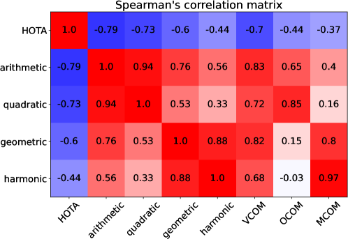
We present the four variations of MOTCOM in Figure 11 computed on the combined MOT17 and MOT20 test splits. We see that they all correlate negatively with the HOTA score. However, the arithmetic mean has the strongest negative correlation and it correlates positively with all the sub-metrics. Therefore, we suggest to compute MOTCOM as the arithmetic mean of the sub-metrics.
0..0.2 Complexity Score Plots for MOT17 and MOT20
In the main paper we evaluate MOTCOM, density, and tracks on the MOT17 and MOT20 test splits. We focus mainly on the ranking capabilities of the metrics as we expect tracker performance to have a monotonic, but not necessarily linear, relationship with complexity. The ranks of MOTCOM, density, and tracks presented in the main paper are based on the scores displayed in Figure 12.
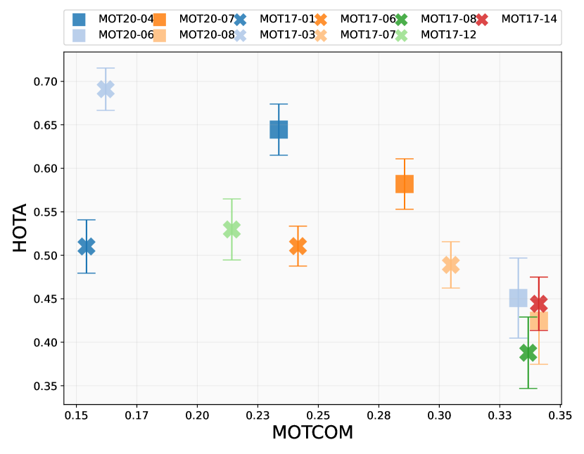
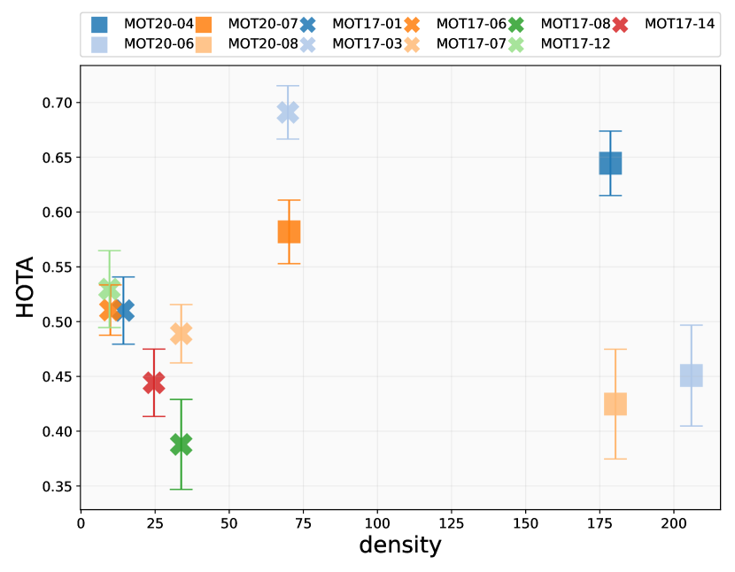
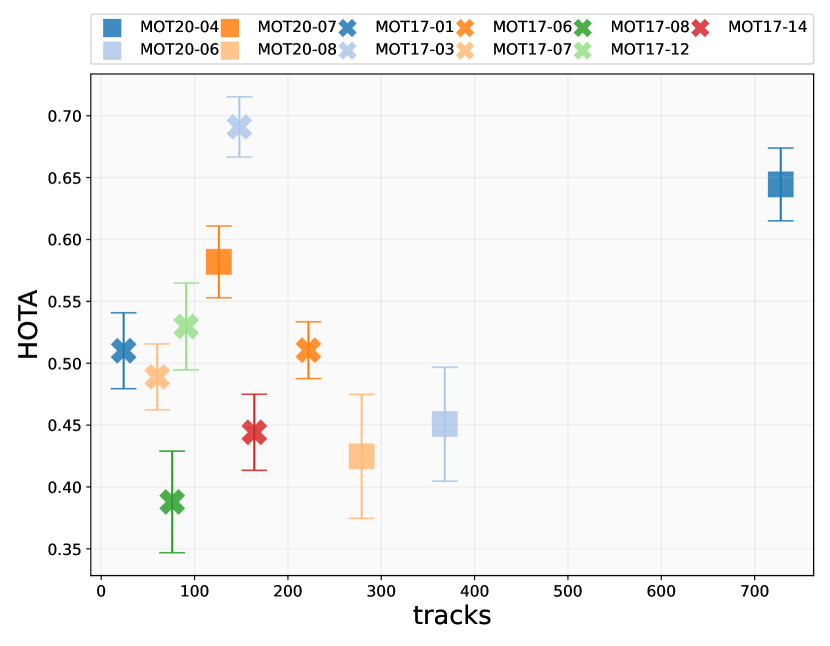
The position of the marker indicates the average score and the error bar is the standard deviation. The marker of the MOT17 sequences is a cross and the MOT20 sequences are represented by a square. We see that the MOT20 sequences have significantly higher densities and more tracks compared to the MOT17 sequences, but the HOTA performance is not correspondingly low. This illustrates that density and tracks do not suffice to describe the complexity of MOT sequences.
0..0.3 Complete Spearman’s Correlation Matrix for MOT17 and MOT20.
In Figure 9 in the main paper we presented a partial Spearman’s correlation matrix based on the MOT17 and MOT20 sequences. We used the matrix to evaluate the monotonic relationship between the three complexity metrics (MOTCOM, density, and tracks) and HOTA, MOTA, and IDF1. In Figure 13 we present the complete Spearman’s correlation matrix, which shows additional details on the relationship between the entries.
0..0.4 Complete Spearman’s Correlation Matrix for MOTSynth.
In the main paper we presented the Spearman’s Footrule Distance and the complexity scores for the MOTSynth sequences. To expand upon this, we include the complete Spearman’s correlation matrix for the MOTSynth train split in Figure 14. The matrix gives a detailed overview of the monotonic relationship between the entries.
