Confident Adaptive Language Modeling

Abstract

Recent advances in Transformer-based large language models (LLMs) have led to significant performance improvements across many tasks. These gains come with a drastic increase in the models’ size, potentially leading to slow and costly use at inference time. In practice, however, the series of generations made by LLMs is composed of varying levels of difficulty. While certain predictions truly benefit from the models’ full capacity, other continuations are more trivial and can be solved with reduced compute. In this work, we introduce Confident Adaptive Language Modeling (CALM), a framework for dynamically allocating different amounts of compute per input and generation timestep. Early exit decoding involves several challenges that we address here, such as: (1) what confidence measure to use; (2) connecting sequence-level constraints to local per-token exit decisions; and (3) attending back to missing hidden representations due to early exits in previous tokens. Through theoretical analysis and empirical experiments on three diverse text generation tasks, we demonstrate the efficacy of our framework in reducing compute—speedup of up to $\times 3$—while provably maintaining high performance.

1 Introduction

Recent advances in Large Language Models (LLMs) have led to breakthroughs in language understanding and language generation across almost every widely-used Natural Language Processing (NLP) task considered in the field today [5; 15; 17; 20; 51; 52; 53; 75; 89; 73]. Autoregressive language modeling provides a flexible framework for solving complex tasks with a unified natural language input and output format, while also relaxing the need for large-scale task-specific data collection and training [67; 15; 17; 58; 80]. The large size of LLMs, however, results in massive computational load that might be limiting for certain real-world applications (e.g., machine translation) [9; 30; 42; 49; 59; 63; 71]. This is especially pronounced in the autoregressive decoding process where the full stack of Transformer layers is repeatedly computed for each output token [37; 40; 86].

While large models do better in general, the same amount of computation may not be required for every input to achieve similar performance (e.g., depending on if the input is easy or hard) [66]. Early exiting is a promising approach to decreasing the computational cost of multilayered architectures such as those used in Transformer-based LLMs, where the number of layers used by the model is dynamically decided on an input-by-input basis [18; 23; 57; 60; 70]. In this setting, an LLM can choose to generate a new token based off the representation at an intermediate layer instead of using the full model, and save computation as a result. A natural question that arises, however, is when is it a good decision to exit early, as opposed to wait? Naively choosing when to exit can be suboptimal in terms of saving computation time, and also result in unpredictable degradations to model performance, especially when predictions depend on each other, as in autoregressive language generation.

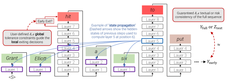
In this work, we analyze the early exiting paradigm for LLMs, and present a principled method for increasing model efficiency while remaining confident in the quality of the resulting predictions. Specifically, we develop a method for calibrating local, per-token, exit decisions such that global, sequence-level constraints—as determined by lexical or semantic sequence-level metrics like ROUGE or BLEURT score—are provably maintained with arbitrarily high probability (e.g., 95%). This process, which we call Confident Adaptive Language Modeling (CALM), is illustrated in Figure 1.

Our approach leverages recent techniques in distribution-free risk control in order to create confident generations with strong statistical guarantees [2; 3; 10]. Concretely, suppose we have been given a calibration set $\mathcal{S}_{\mathrm{cal}}:=\{P_{i}\}_{i=1}^{n}\in\mathcal{P}^{n}$ of independent and identically distributed (i.i.d.) prompts to our LLM (e.g., paragraphs to be summarized, sentences to be translated, or questions to be answered via language modeling). Let $P_{\mathrm{test}}$ be a new i.i.d. test prompt to our LLM, where $Y_{\mathrm{early}}:={\text{LLM}}_{\mathrm{early}}(P_{\mathrm{test}})$ and $Y_{\mathrm{full}}:={\text{LLM}}_{\mathrm{full}}(P_{\mathrm{test}})$ are the adaptive and standard outputs of our LLM, respectively. In order to be satisfied with $Y_{\mathrm{early}}$, we might require it to be textually consistent with $Y_{\mathrm{full}}$. Given any bounded text dissimilarity function $\mathcal{D}$, we aim to calibrate the early-exiting LLM such that its predictions agree to a tolerance $\delta$ with the full model in expectation with high probability,

$$\mathbb{P}\Big{(}\mathbb{E}\big{[}\mathcal{D}(Y_{\mathrm{early}},Y_{\mathrm{full}})\big{]}\leq\delta~{}\big{|}~{}\mathcal{S}_{\mathrm{cal}}\Big{)}\geq 1-\epsilon,$$ (1)

where the randomness is over draws of $\mathcal{S}_{\mathrm{cal}}$, and $\epsilon\in(0,1)$. Eq. (1) has the significant advantage of being achievable using only unlabeled calibration data $\mathcal{S}_{\mathrm{cal}}$ (a quality that is critical for few-shot tasks, for example). Enforcing textual consistency with the original $Y_{\mathrm{full}}$, however, may be unnecessarily strict for certain tasks, especially where multiple generations may be acceptable. As an alternative, given a calibration set of prompts paired with a set of (potentially multiple) target references, $\mathcal{S}_{\mathrm{cal}}:=\{(P_{i},Z_{i})\}_{i=1}^{n}\in(\mathcal{P}\times 2^{\mathcal{Y}})^{n}$, and any bounded risk function $\mathcal{R}$, we also consider an objective that enforces risk consistency by limiting the relative increase in risk of the predictions $Y_{\mathrm{early}}$ compared to $Y_{\mathrm{full}}$, with respect to the set of test-time references $Z_{\mathrm{test}}$, i.e.,

$$\mathbb{P}\Big{(}\mathbb{E}\big{[}\mathcal{R}(Y_{\mathrm{early}},Z_{\mathrm{test}})-\mathcal{R}(Y_{\mathrm{full}},Z_{\mathrm{test}})\big{]}\leq\delta~{}\big{|}~{}\mathcal{S}_{\mathrm{cal}}\Big{)}\geq 1-\epsilon.$$ (2)

Within the constraints of either Eq. (1) or Eq. (2), the goal of our work is to find the most computationally efficient $Y_{\mathrm{early}}$, i.e., generations that exit as early as possible while still maintaining our desired performance guarantees. In order to achieve this, it is necessary to develop a reliable signal for how likely local, per-token early-exit decisions are to disrupt the global properties of the complete sequence. Here, we first analyze how errors are propagated in Transformer-based LLMs, and then present an effective and efficient scoring mechanism for assigning “consistent early-exit” confidence scores after each layer used during the generation of a new token. The decision to exit or not is based on these scores, and is carefully calibrated using $\mathcal{S}_{\mathrm{cal}}$ such that our performance bounds are provably satisfied.

Finally, we empirically validate our method on multiple, diverse NLP generation tasks, including text summarization, machine translation, and question answering. Our experiments demonstrate the potential of CALM in reducing the average complexity of the model and accelerating inference by about $\times 3$ while reliably controlling for high performance.

Figure 1: Illustration of CALM generation (see Figure 4 for the full example) with local per-token early exiting decisions that provably satisfy global user-defined constraints on the full sequence.

Contributions. In summary, our main contributions are as follows:

• A framework (CALM) for reliably accelerating Transformer-based LLM generations.

• A systematic analysis of the token-wise early exit mechanism that motivates a simple-but-effective class of confidence measures and threshold functions that are used as part of the CALM framework.

• An empirical demonstration of CALM’s efficiency gains on three diverse generation datasets.

2 Related Work

Improving inference-time efficiency of LLMs has been an ongoing effort of the research community over the past several years [49; 72; 85], leveraging techniques such as knowledge distillation [6; 32; 36; 69; 69; 78; 56], floating point quantization [71; 65], layer pruning [24], vector dropping [38], and others [41]. Another line of work involves conditional computation to train larger models that only use a sparser subset of the full network during inference, for example by routing over mixture-of-experts [9; 22; 39; 91], recurring modules [18; 29; 35], or accessing external memory [82]. These models, however, still use the same amount of compute for all input examples.

Here, we focus on adaptive compute, a specific kind of conditional compute that aims to dynamically allocate different computational power per example, with the goal of reducing the overall complexity while maintaining high performance. This approach, often referred to as early-exiting [16; 25; 47; 74; 79; 87], is complementary to many of the solutions above and can potentially be combined with them. Multiple early-exit techniques for encoder-only Transformers (e.g., BERT [20]) have been recently proposed [8; 34; 43; 44; 45; 60; 68; 83; 90; 92]. Most of these methods rely on intrinsic confidence measures (e.g., based on the softmax distribution), while others try to predict the routing in advance [46; 70], or train a small early-exit classifier [57; 84], as we also examine here. These measures can be calibrated to reliably guarantee consistency of the early prediction with the full model [57]. However, the techniques used for encoder-only classifiers are unsuitable for global consistency constraints with a sequence of dependent predictions, which are inherent in the decoding process of autoregressive language models, which we address here.

Our work is also motivated by recent findings on the existence of saturation events in LMs, where the top-ranked prediction is unchanged after some layer and is propagated upward. Geva et al. [28] examined interactions of the hidden-state with feed-forward layers to predict these events. However, they only consider local single predictions and do not address the challenges involved with sequence generation. Our early-exit LM architecture most closely relates to Elbayad et al. [23], who found a token-level early-exit classifier to provide the best efficiency-performance tradeoffs on machine translation. Here, we introduce a theoretically-grounded calibration method for provably controlling the quality of the full sequence. By doing so, we provide reliable efficiency gains—deriving local early exiting decisions from the global desirable constraints. Moreover, we introduce several model improvements and empirical analyses, including (1) analyzing the primary sources of performance degradation, leading us to propose a decaying threshold function for better tradeoff control without inflating the search space; (2) improving the early-exit classifier training; and (3) experimenting with two new tasks.

Our calibration procedure for connecting global constraints to local decisions, relates to recent research around distribution-free uncertainty quantification [1; 62; 77]. Several methods were developed in recent studies to expand and adjust the theoretical framework for obtaining practical efficiency gains on target applications [4; 7; 21; 26; 27; 48; 88]. Here, we frame our consistency requirements around the Learn then Test (LTT) framework [3], and leverage the approximately monotonic behavior of our confidence measures and the nested structure of our problem, that by definition guarantees consistency with large enough threshold, to form tight and effective bounds.

3 Early Exiting for Adaptive Language Modeling

In the following, we describe and analyze the early-exiting Transformer LM. We begin with a brief recap of the Transformer architecture (§3.1) and early exiting (§3.2) for convenience, following previous work [23; 70; 76]. We then investigate the effects of early exiting on model performance, and identify primary sources of performance degradation and how to alleviate them (§3.3)—which guide our architecture and training design (§3.4) and proposed per-token confidence measures (§3.5).

3.1 The Transformer architecture

We use the Transformer sequence-to-sequence model, based on the T5x implementation [55]. Here, we only review simplified details of the Transformer architecture relevant to early-exiting, and refer the reader to Vaswani et al. [76] for full details. At a high level, both encoder and decoder networks contain $L$ stacked layers, where each layer is composed of a multi-head self-attention sub-layer, followed by a feedforward sub-layer, each with residual connections and layer normalization. The decoder network has an additional multi-head attention sub-layer that attends to the encoder states.

Consider a prompt $x=(x_{1},\ldots,x_{p})$, processed by the encoder to yield encoder states $(e_{1},\ldots,e_{p})$, and the current, partially generated response $(y_{1},\ldots,y_{t})$. When generating the next token $y_{t+1}$, the decoder computes a decoder state $d_{t}^{i}$ for layer $i$ out of $L$ as:

$$h_{t}^{i}:=\mathrm{Attention}(d_{t}^{i-1},d_{1:t-1}^{i-1});\hskip 10.0pta_{t}^{i}:=\mathrm{Attention}(h_{t}^{i},e_{1:p});\hskip 10.0ptd_{t}^{i}:=\mathrm{FeedForward}(a_{t}^{i}).$$ (3)

Internal to each of the attention mechanisms, written as $\mathrm{Attention}(x,z_{1:m})$ for some input $x$ and sequence of $m$ states $z_{1:m}$, $x$ is first projected to a query vector $q:=\mathbf{W}_{Q}x\in\mathbb{R}^{\mathrm{dim}_{k}}$, while $z$ is projected to a matrix of key-value vectors, $\mathbf{K}:=\mathbf{W}_{K}z_{1:m}\in\mathbb{R}^{m\times\mathrm{dim}_{k}}$ and $\mathbf{V}:=\mathbf{W}_{V}z_{1:m}\in\mathbb{R}^{m\times\mathrm{dim}_{v}}$. The output $o$ is then computed as $o:=\mathrm{softmax}\left(q\mathbf{K}^{\top}/\sqrt{\mathrm{dim}_{k}}\right)\mathbf{V}$.

Multi-head and normalization components are omitted for brevity. Each layer uses different projections $\mathbf{W}^{i}_{Q}$, $\mathbf{W}^{i}_{K}$, and $\mathbf{W}^{i}_{V}$ (which are also unique for computing $h_{t}^{i}$ versus $a_{t}^{i}$).

Finally, after layer $L$, a distribution over vocabulary tokens $y_{t+1}\in\mathcal{Y}$ is computed via a softmax-normalized linear classifier $\mathbf{W}_{L}$, where $p(y_{t+1}\mid d_{t}^{L})=\mathrm{softmax}(\mathbf{W}_{L}d_{t}^{L})$.

3.2 Decoding with early exiting

Instead of always making a prediction based on the representation at the final layer, $d_{t}^{L}$, the key idea in early-exiting is to choose $y_{t+1}$ more quickly, if confident, by computing $p(y_{t+1}\mid d_{t}^{i})=\mathrm{softmax}(W_{i}d_{t}^{i})$ for some intermediate layer $i<L$. Concretely, let $c_{t}^{i}\in[0,1]$ denote some local confidence score for layer $i$ while processing token $t$, where higher values indicate a higher propensity to exit early (we will propose effective instantiations of $c_{t}^{i}$ in §3.5). Let $\lambda_{t}^{i}\in[0,1]$ denote some local early-exiting threshold, where the model exits early if $c_{t}^{i}\geq\lambda_{t}^{i}$, or otherwise proceeds to compute the next representation, $d_{t}^{i+1}$. The (greedily chosen) prediction $y_{t+1}$ can then be written as:

$$\small y_{t+1}:=\left\{\begin{array}[]{@{}l@{\thinspace}l}\operatorname*{arg\,max}p(y_{t+1}~{}|~{}d_{t}^{1})&\hskip 17.07164pt\text{if }c_{t}^{1}\geq\lambda_{t}^{1},\\[2.0pt] \operatorname*{arg\,max}p(y_{t+1}~{}|~{}d_{t}^{2})&\hskip 17.07164pt\text{if }c_{t}^{2}\geq\lambda_{t}^{2},\\[2.0pt] \phantom{\operatorname*{arg\,max}p(y_{t+1}~{}}\vdots\\[2.0pt] \operatorname*{arg\,max}p(y_{t+1}~{}|~{}d_{t}^{L})&\hskip 17.07164pt\text{otherwise}.\\ \end{array}\right.$$ (4)

Note that due to the self-attention mechanism of the Transformer, computing the input hidden state $h_{t}^{i}$ for layer $i$ depends on $d_{1:t-1}^{i-1}$, i.e., the output hidden states of the previous layer for all the tokens that have been generated so far. Therefore, if the model has early exited at some layer $j<{i-1}$ for a token $s<t$, then $d_{s}^{i-1}$ is not available. As an approximation, we set $d_{s}^{k}=d_{s}^{j}$ for all layers $k>j$ following Elbayad et al. [23], with the understanding that this will introduce some error. In the next section, in addition to other factors, we will analyze the impact of this copied state on performance.

3.3 The effects of early exiting on error propagation

We perform several controlled experiments to investigate the behavior and the potential of early-exiting during decoding. We use an 8-layer T5 encoder-decoder and the CNN/DM dataset for these experiments. See §5 for more details on this model and data.

3.3.1 State propagation

First, we control for the correctness of the predicted tokens to examine the effect of state copying (§3.2), and also measure an approximate upper bound for compute reduction. We use an oracle confidence measure that exits at the earliest layer that agrees with the top prediction (i.e., replacing the conditions in Eq. 4 with $\operatorname*{arg\,max}p(y_{t+1}~{}|~{}d_{t}^{i})=\operatorname*{arg\,max}p(y_{t+1}~{}|~{}d_{t}^{L})$). Hence, the only factor that can cause divergence in the generation is the state copying mechanism for skipped layers. The results of this experiment are highly encouraging. This oracle achieves an ROUGE-L score of 38.24, compared to 38.32 with the full model, while only using an average of 1.53 layers per token. We also try an oracle that always uses $d^{1}_{1:t-1}$ and it reaches 38.31 ROUGE-L. These results indicate that (1) the model is robust to state copying from lower layers, and (2) there is remarkable potential for saving compute—by up to $\times 5.2$—while preserving performance, given a good confidence measure.

We also experiment with copying the projected states $\mathbf{K}^{j},\mathbf{V}^{j}$ to skipped layers $k>j$. This version of the oracle results in a significant drop in performance to 23.02 ROUGE-L. Overall, we conjecture that the self-attention at layer $i$ for token $t$ can safely use hidden-states $d^{j}_{s}$ for $j<i-1$ as key-values of tokens $s<t$, as long as the projections $\mathbf{W}^{i}_{K/V}$ of layer $i$ are used. Notably, this projection can now be computed concurrently for all skipped layers as they all use the same $d$ from the exited layer.

3.3.2 Sensitivity to local errors

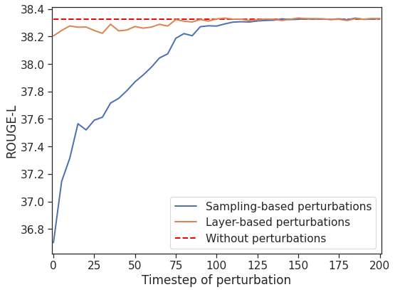
Next, we examine the impact of local token modifications—which might occur due to early exits—on the whole generated sequence. We experiment with two kinds of perturbations: sampling-based, where we select the 10th-ranked token according to layer $L$; and layer-based, where we select the the first layer’s prediction at timestep $t$. All other tokens are predicted greedily by layer $L$. As shown in Figure 2(a), earlier perturbations result in lower sequence-level scores as there are more tokens that might suffer from the divergence. The degradation, though, is much smaller with layer- compared to sampling-based perturbations since, in practice, the early exit predictions are mostly accurate.

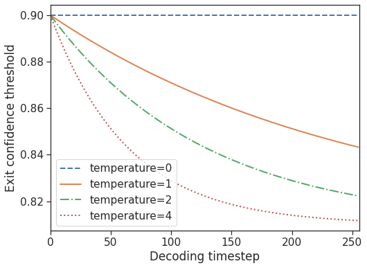
Decaying threshold. Following the above observation, we introduce a decaying early-exiting threshold that is more permissive towards exiting as the decoding process continues. Motivated by the logarithmic behavior in Figure 2(a), we use an exponential function with a user-defined temperature $\tau$:

$$\small\lambda^{\prime}(\lambda,t):=\mathrm{clip}_{[0,1]}\left(\frac{9}{10}\lambda+\frac{1}{10}e^{-\tau\cdot t/N}\right),$$ (5)

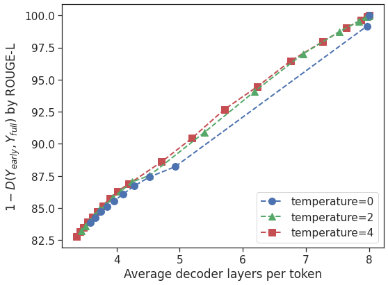
where $N$ is the maximum output length. Figure 2(b) illustrates this function. Essentially, this function presents an effective compromise between simply using the same threshold for all tokens, and searching over a huge space of per-position different thresholds. Practically, it supports finer and better control over the performance-efficiency tradeoff compared to a single threshold. Figure 2(c) presents the outcomes of a search over $\lambda$ with steps of $0.01$ and softmax-based confidence (§3.5). With the single threshold variant ($\tau=0$), attempting to improve the efficiency will lead to a drastic drop of more than 10 points in the textual similarity against the full model’s prediction. In contrast, the decaying thresholds reveal several intermediate points with desirable tradeoffs to consider.

(a) Sensitivity to local errors.

(b) Decaying threshold ($\lambda=0.9$).

(c) Perf.-efficiency tradeoffs.

Figure 2: Earlier noise in the decoding process has greater effect on the overall output (a), though in practice the affect of early exits is minor due to high performance of early layers. A decaying confidence threshold (b) allows finer control over the performance-efficiency tradeoff (c).

3.4 Training early exit classifiers for local consistency

While our goal is to preserve the quality of the complete output sequence, we note that this doesn’t necessarily demand local token-level consistency. Consider the target sequence “the concert was wonderful and long.” An output that switches the order of adjectives to “the concert was long and wonderful” would be called consistent by most semantic measures (and obtain 100 token-$F_{1}$ score). Yet, the sentences diverge at the first adjective long which is semantically different from wonderful.

Training for global consistency, however, could be challenging [81] as it depends on possibly noisy signals that might affect the learning, and also breaks the efficient teacher-forcing training strategy of LMs that relies on local-decisions. On the other hand, perfect local consistency implies global consistency. Therefore, we opt to train for local consistency, which requires minimal changes to the training procedure, and relax the local requirement to a global one during inference.

Specifically, similar to Elbayad et al. [23], we average losses for each layer to obtain the objective

$$\small\mathcal{L}=\sum_{i=1}^{L}{\omega_{i}}\mathcal{L}_{i},\quad\text{where}\quad\sum_{i=1}^{L}\omega_{i}=1.$$ (6)

$\mathcal{L}$ is the negative log-likelihood loss. We set $\omega_{i}=i/{\sum_{j=1}^{L}j}$ to favor higher layers, and find this objective to mostly preserve the full model’s performance compared to regular training. We note that there is some misalignment between this training and inference behavior due to the hidden states of skipped layers. However, as discussed in §3.3.1, the performance is not affected if the hidden-state is copied.

3.5 Local confidence measures

We experiment with three confidence measures for Eq. (4) that differ in their parameter and compute operation efficiencies. Our experiments (§6) will also show that they differ in their predictive power.

Softmax response. We take the difference between the top two values of $\operatorname{Softmax}(\mathbf{W_{i}}d^{i}_{t})$. With a large output vocabulary, this results in many floating point operations (FLOPs)—though, the next layer $i+1$ can start its computation in parallel, avoiding additional runtime.

Hidden-state saturation. As a simple parameter-free and fast to compute alternative, we take the cosine similarity $\mathrm{sim}(d^{i}_{t},d^{i-1}_{t})$ for $i>1$. By definition, the first possible exit is at the second layer (unless $\lambda=0$). This measure tries to identify early saturation events of the hidden-state [28].

Early exit classifier. We train a dedicated linear classifier $\mathcal{M}$ to predict the likelihood of exiting with local consistency given the current hidden-state: $c_{t}^{i}=\mathcal{M}(d_{t}^{i})$. This measure is very fast to compute at inference, and adds only $|d|+1$ new parameters. To avoid any impact on the core model’s performance, we train it as a second step where we freeze all parameters other than $\mathcal{M}$. We simply use a per-layer independent cross-entropy loss against a consistency oracle $\mathbbm{1}[\operatorname*{arg\,max}(p(y_{t+1}|d_{t}^{i})=\operatorname*{arg\,max}(p(y_{t+1}|d_{t}^{L})]$, and average across the $L-1$ layers. We also experimented with the geometric-like training of Elbayad et al. [23], but find it to be less effective here (see App. D). The two objectives are closely related, but the geometric one ignores any signal from the states post the first oracle exit.

4 Calibrating Local Early Exits from Global Constraints

We now describe our calibration procedure for finding a shared exit threshold $\lambda\in[0,1]$ that can be used directly in Eq. (4), or via Eq. (5), such that we provably satisfy our desired global constraints over the fully generated sequences. At a high level, our approach uses the following basic recipe:

1. We specify a grid of possible values of $\Lambda=(\lambda_{1},\ldots,\lambda_{k})$ that may result in acceptable generations;

2. We choose the lowest valid $\lambda\in\Lambda$ that we can identify with rigorous statistical testing tools.

Let $P_{\mathrm{test}}$ be an i.i.d. prompt given to the LLM at test time, and let $Y_{\mathrm{full}}:=\text{LLM}_{\mathrm{full}}(P_{\mathrm{test}})\in\mathcal{Y}$ and $Y_{\mathrm{early}}:=\text{LLM}_{\mathrm{early}}(P_{\mathrm{test}},\lambda)\in\mathcal{Y}$ denote the full and adaptive responses, respectively. Optionally, let $Z_{\mathrm{test}}$ be a set of gold references for our task, if assumed. Our goal, as introduced in §1, is to find a valid $\lambda$ using $\mathcal{S}_{\mathrm{cal}}$ such that we satisfy either of two types of global “consistency” constraints:

Definition 1 (Textual consistency).

An adaptive LLM is textually consistent if given any bounded text dissimilarity function, $\mathcal{D}\colon\mathcal{Y}\times\mathcal{Y}\rightarrow\mathbb{R}$, and tolerance $\delta\in\mathbb{R}$, $\mathbb{E}\big{[}\mathcal{D}(Y_{\mathrm{early}},Y_{\mathrm{full}})\big{]}\leq\delta$.

Definition 2 (Risk consistency).

An adaptive LLM is risk consistent if given any bounded risk function, $\mathcal{R}\colon\mathcal{Y}\times 2^{\mathcal{Y}}\rightarrow\mathbb{R}$, and tolerance $\delta\in\mathbb{R}$, $\mathbb{E}[\mathcal{R}(Y_{\mathrm{early}},Z_{\mathrm{test}})]\leq\mathbb{E}[\mathcal{R}(Y_{\mathrm{full}},Z_{\mathrm{test}})]+\delta$.

Without loss of generality, we will assume that $\mathcal{D}$ and $\mathcal{R}$ are always normalized to the unit interval $[0,1]$, and therefore will only be considering tolerances $\delta\in(0,1)$. At a glance, to find a $\lambda$ that produces a consistent $\text{LLM}_{\mathrm{early}}$, we cast our problem as a multiple hypothesis testing problem over a large array of $k$ candidate classifier exit thresholds, $\Lambda=(\lambda_{1},\ldots,\lambda_{k})$, and apply the Learn then Test (LTT) framework of Angelopoulos et al. [3] to identify a subset of statistically valid, constraint-satisfying thresholds $\Lambda_{\textrm{valid}}\subseteq\Lambda$. Our final $\lambda$ is then chosen as $\lambda:=\min(\Lambda_{\textrm{valid}}\cup\{1\})$.

4.1 The Learn then Test calibration framework

Choosing a value of $\lambda$ that rigorously satisfies our consistency objectives is challenging, as the performance impact of increasing or decreasing $\lambda$ is not necessarily monotonic. Naively setting $\lambda$, for example, based simply on average calibration set performance, can lead to statistically invalid results in our finite-sample, distribution-free setting. The LTT framework proposed by Angelopoulos et al. [3] solves this problem by reframing hyper-parameter selection as a multiple testing problem.

Let $\Lambda=(\lambda_{1},\ldots,\lambda_{k})$ be a finite grid of hyper-parameter values that may, or may not, obtain valid consistency. For example, when searching for a value of $\lambda\in[0,1]$, we might consider the evenly spaced set $\Lambda=\{\frac{i}{k+1}\colon i=1,\ldots,k\}$. LTT then identifies a subset of values, $\Lambda_{\mathrm{valid}}\subseteq\Lambda$, where

$$\mathbb{P}\Big{(}\exists{\lambda}\in\Lambda_{\mathrm{valid}}\colon\text{LLM}_{\mathrm{early}}(P_{\mathrm{test}},{\lambda})\text{ and }\text{LLM}_{\mathrm{full}}(P_{\mathrm{test}})\text{ are {not} consistent }\Big{)}\leq\epsilon.$$ (7)

Here, we are using consistency to refer to either textual consistency or risk consistency. Eq. (7) can be satisfied by applying standard multiple hypothesis testing techniques as long as super-uniform p-values, $p_{j}$, are supplied for each value $\lambda_{j}\in\Lambda$ that support the null hypothesis

$${H}_{j}\colon\text{LLM}_{\mathrm{early}}(P_{\mathrm{test}},\lambda_{j})\text{ and }\text{LLM}_{\mathrm{full}}(P_{\mathrm{test}})\text{ are {not} consistent.}$$ (8)

$\lambda_{j}$ is placed in $\Lambda_{\mathrm{valid}}$ if ${H}_{j}$ is rejected, and discarded otherwise. This yields a consistent $\text{LLM}_{\mathrm{early}}$.

Proposition 1 (LTT for CALM).

Suppose $p_{j}$ is super-uniform for all $j$ under ${H}_{j}$ for some specified tolerance $\delta\in(0,1)$. Let $\mathcal{A}$ be any family-wise error rate (FWER) controlling procedure at a level $\epsilon\in(0,1)$, where $\mathcal{A}(p_{1},\ldots,p_{k})$ selects $H_{j}$ to reject. Choosing $\lambda:=\min(\Lambda_{\mathrm{valid}}\cup\{1\})$ then yields a consistent $\text{LLM}_{\mathrm{early}}$ with probability at least $1-\epsilon$.

Note that a FWER-controlling procedure at a level $\epsilon$ is an algorithm that decides to accept or reject hypotheses $\{H_{i}\}_{i=1}^{k}$, while ensuring that the probability of falsely rejecting any $H_{j}$ is less than $\epsilon$. The proof of Proposition 1, given in Appendix A.1, follows directly from Theorem 1 of Angelopoulos et al. [3], and the fact that $\text{LLM}_{\mathrm{{early}}}(P_{\mathrm{test}},1)=\text{LLM}_{\mathrm{full}}(P_{\mathrm{test}})$ by construction per Eq. (4), so that we can always use $\lambda=1$ as a valid fallback if we fail to identify non-empty $\Lambda_{\mathrm{valid}}$. In the next sections, we describe how we calculate valid p-values using $\mathcal{S}_{\mathrm{cal}}$, and our choice of FWER-controlling procedure.

4.2 Defining p-values for consistent early-exiting

LTT relies on valid p-values $p_{j}$, where $p_{j}$ is a random variable satisfying $\mathbb{P}(p_{j}\leq u)\leq u$ under $H_{j}$ for all $u\in[0,1]$. For our purposes, we can obtain valid p-values from the empirical consistency of $\text{LLM}_{\mathrm{early}}(P_{i},\lambda)$ measured over the random calibration sample, $\mathcal{S}_{\mathrm{cal}}$. Since we have assumed w.l.o.g. that either of our bounded consistency functions $\mathcal{D}$ and $\mathcal{R}$ from Defs. 1 and 2 have been normalized to lie in $[0,1]$, we can, for example, obtain a valid p-value by simply inverting Hoeffding’s inequality:

$$p_{j}^{\text{Hoeffding}}:=e^{-2n(\max(0,\delta-\widehat{E}(\lambda_{j})))^{2}},$$ (9)

where $\widehat{E}(\lambda_{j}):=\frac{1}{n}\sum_{i=1}^{n}L_{i}(\lambda_{j})$ is the empirical average of random variable $L_{i}(\lambda_{j})\in[0,1]$, with

$$L_{i}(\lambda_{j}):=\mathcal{D}(\text{LLM}_{\mathrm{{early}}}(P_{i},\lambda_{j}),\text{LLM}_{\mathrm{{full}}}(P_{i}))\quad\text{or}$$ (10)

$$L_{i}(\lambda_{j}):=\max\left(0,\mathcal{R}(\text{LLM}_{\mathrm{{early}}}(P_{i},\lambda_{j}),Z_{i})-\mathcal{R}(\text{LLM}_{\mathrm{{full}}}(P_{i}),Z_{i})\right),$$ (11)

for textual consistency versus risk consistency, respectively. Note that, as a technicality of enforcing the r.v. $L_{i}(\lambda_{j})$ to be within $[0,1]$, Eq. (11) computes a conservative estimate of the difference in the empirical risk that doesn’t reward instances in which the risk of the early-exit model is lower.

4.3 Efficient fixed sequence testing

The more values of $\lambda$ we test, the higher the chance that we might accidentally choose a $\lambda$ that does not in fact result in consistent generations, despite whatever misleading performance we might have measured by chance on $\mathcal{S}_{\mathrm{cal}}$. As part of LTT, we must select a multiple testing procedure that corrects for this (i.e., that controls the FWER at level $\epsilon$). Though the precise dependence between the early-exit LLM’s performance and $\lambda$ is unknown, in practice we find that it tends to be fairly smooth and roughly monotonic. That is, nearby thresholds $\lambda\approx\lambda^{\prime}$ tend to perform similarly, whereas $\lambda>\lambda^{\prime}$ tends to result in relatively more consistent performance. Taking advantage of this structure, we choose to employ fixed sequence testing (FST) as our FWER-controlling procedure [3; 11].

Here we define a sequence of descending thresholds $\lambda_{1}>\lambda_{2}>\ldots\lambda_{k}$ with a relatively coarse step size (e.g., increments of $0.05$). For each $\lambda_{j}$ in order, we compute $p_{j}$, and reject $H_{j}$ if $p_{j}\leq\epsilon$. The first time we fail to reject $H_{j}$, we immediately terminate our search, and return $\lambda_{j-1}$ to use as our calibrated threshold (or $1$, if we fail to reject $H_{1}$). An Algorithm of the full procedure is provided in Appendix E.

5 Experimental Setting

Table 1: Average number of tokens in reference targets of evaluation datasets (5/95th percentiles in parenthesis).

Dataset	Output length
CNN/DM	82 (42 - 141)
WMT EN-FR	39 (10 - 82)
SQuAD	5 (1 - 13)

We empirically evaluate our methods on three popular text generation tasks that vary in their target generation length and extractive degrees against the input. CNN/DM [31] is a collection of news articles to be summarized in few sentences. WMT15 EN-FR [13] contains English sentences (one per example) to be machine translated to French. Open-book SQuAD 1.1 [54] is a QA dataset with Wikipedia paragraphs paired with questions, where the target answer is a text span from the input. Length statistics of the validation sets are summarized in Table 1.

Model. We implement CALM on top of the T5 encoder-decoder model that showed good performance on the tasks above [53], using the T5X framework [55]. We use the 8 layers T5 1.1 model that doesn’t share input and output embeddings. We share all output embeddings for the softmax predictions, and the early-exit classifier across all decoder layers. Based on validation results, we set the temperature of our decaying threshold to $\tau=4$ for the softmax and classifier measures of CNN/DM and WMT. In other settings, we use $\tau=0$. See App. C for more details, and App. B.3 for a 12 layers T5 model.

Evaluation metrics. We use the standard metrics for each task: ROUGE-L for CNN/DM, BLEU [50] for WMT, and Token-F1 [54] for SQuAD. We rely on the same metrics for computing the risk and textual distance, other than BLEU which is a corpus-level metric that doesn’t directly enable expectation control. Instead, we use the BLEURT learned metric [61]. For a given metric $m(y_{\mathrm{early}},y_{\mathrm{full}}\mathrm{\ or\ }z_{\mathrm{test}})\in[0,1]$, we use $1-m$ for distance or risk computation, respectively.

Our main efficiency metric is the average number of decoder layers used per output token, as it directly measures complexity reduction without conflating with implementation or infrastructure specific details [19]. For reference, we also report the average decoder FLOPs reduction per token [23]. Also, we compute an estimated speedup of the whole encoder-decoder model for generating the full sequence, based on TPUv3 benchmarking with 200 examples in Colab (see App. C for details).

Calibration experiments. For each task, we use the validation and test sets to evaluate our calibration method (§4) (for SQuAD we only use the validation set as the test answers are hidden). We run 50 random trials per target tolerance $\delta$ and consistency objective (textual or risk), where we partition the data to 80% calibration ($\mathcal{S}_{\mathrm{cal}}$) and 20% test ($P_{\mathrm{test}}$). We set $\epsilon=0.05$ for all experiments.

Baselines. We emphasize that the CALM framework is general for any autoregressive multi-layered LM with any confidence measure, allowing controlled consistency by Eq. (1) or Eq. (2). To empirically evaluate the efficiency gains enabled by our proposed confidence measures, we compare with static baselines that use the same number of layers for all tokens. We also compare our early-exit classifier training with the geometric method of [23] in Appendix D. Also, we compute an oracle local measure (§3.3.1) as an upper-bound estimate of the performance-efficiency tradeoff.

6 Experimental Results

(a) CNN/DM

(b) WMT

(c) SQuAD

Figure 3: Validation empirical performance-efficiency tradeoffs for different confidence measures, compared to static baselines and a local oracle measure with state propagation for skipped layers.

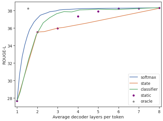
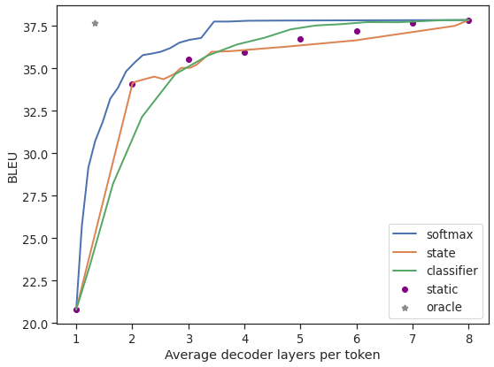
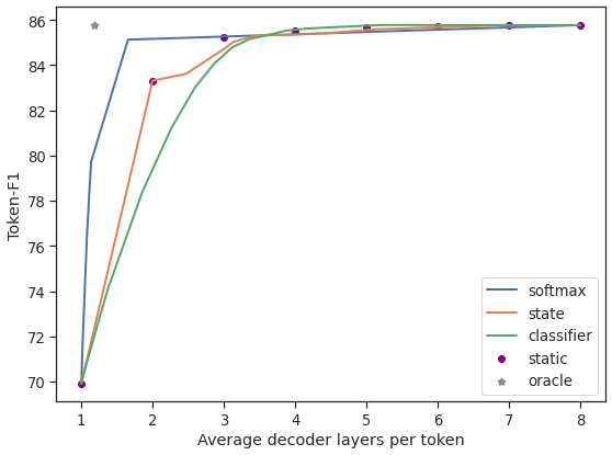
We first report the empirical performance-efficiency tradeoff achieved with each confidence measure. For each task and measure, we evaluate the full range of $\lambda$ on the validation set, with steps of $0.05$. The results, presented in Figure 3, show the power of the softmax response measure, allowing only minor performance loss while reducing more than half of the layers in all three tasks. The early-exit classifier, that is more FLOP-efficient, is also effective, mostly when targeting high performance (right hand side of plots). The simple and parameter-free state saturation measure is competitive, but often falls bellow the static baseline, despite enabling per-token exit decisions.

The dynamic oracle obtains compelling efficiency gains, using only 1.5, 1.3, and 1.2 layers on average for summarization, WMT, and QA, respectively, without losing any performance. This illustrates the full potential of CALM and leaves further room for improvements with better confidence measures. It also shows the effectiveness of inference-time state propagation for skipped layers (§3.3.1).

Table 2: Test efficiency gains per choice of $\delta$, consistency objective, and confidence measure. For plots of the full range of $\delta$ with standard deviation, see Appendix B.

			CNN/DM			WMT			SQuAD
	$\delta$	Measure	layers	FLOPs r.	speedup	layers	FLOPs r.	speedup	layers	FLOPs r.	speedup
Textual consist.	$0.1$	softmax	$\textbf{5}.\textbf{73}$	$\times 0.44$	$\times 1.41$	$\textbf{3}.\textbf{35}$	$\times 0.66$	$\times 2.01$	$\textbf{1}.\textbf{65}$	$\times 3.15$	$\times 1.63$
		state	$8.00$	$\times 1.00$	$\times 1.00$	$7.68$	$\times 1.01$	$\times 1.00$	$2.00$	$\times\textbf{3}.\textbf{65}$	$\times\textbf{1}.\textbf{68}$
		classifier	$7.16$	$\times\textbf{1}.\textbf{03}$	$\times\textbf{1}.\textbf{42}$	$5.50$	$\times\textbf{1}.\textbf{06}$	$\times\textbf{2}.\textbf{05}$	$2.59$	$\times 2.37$	$\times 1.10$
	$0.25$	softmax	$\textbf{2}.\textbf{62}$	$\times 0.49$	$\times\textbf{2}.\textbf{57}$	$\textbf{1}.\textbf{76}$	$\times 0.91$	$\times\textbf{2}.\textbf{83}$	$\textbf{1}.\textbf{03}$	$\times\textbf{5}.\textbf{68}$	$\times\textbf{1}.\textbf{88}$
		state	$7.97$	$\times 1.00$	$\times 1.01$	$2.84$	$\times\textbf{1}.\textbf{93}$	$\times 1.55$	$2.00$	$\times 3.65$	$\times 1.68$
		classifier	$4.51$	$\times\textbf{1}.\textbf{15}$	$\times 2.04$	$2.97$	$\times 1.22$	$\times 2.00$	$1.37$	$\times 5.09$	$\times 1.11$
Risk consist.	$0.02$	softmax	$\textbf{3}.\textbf{75}$	$\times 0.47$	$\times\textbf{1}.\textbf{96}$	$\textbf{3}.\textbf{19}$	$\times 0.67$	$\times\textbf{2}.\textbf{10}$	$\textbf{1}.\textbf{65}$	$\times\textbf{3}.\textbf{15}$	$\times 1.63$
		state	$7.97$	$\times 1.00$	$\times 1.01$	$7.68$	$\times 1.01$	$\times 1.00$	$3.13$	$\times 2.11$	$\times\textbf{1}.\textbf{68}$
		classifier	$6.49$	$\times\textbf{1}.\textbf{06}$	$\times 1.71$	$5.05$	$\times\textbf{1}.\textbf{08}$	$\times 1.97$	$3.36$	$\times 1.55$	$\times 1.11$
	$0.05$	softmax	$\textbf{1}.\textbf{73}$	$\times 0.50$	$\times\textbf{3}.\textbf{53}$	$\textbf{1}.\textbf{96}$	$\times 0.85$	$\times\textbf{2}.\textbf{73}$	$\textbf{1}.\textbf{65}$	$\times 3.15$	$\times 1.63$
		state	$5.22$	$\times 1.11$	$\times 1.64$	$2.72$	$\times\textbf{2}.\textbf{01}$	$\times 1.58$	$2.00$	$\times\textbf{3}.\textbf{65}$	$\times\textbf{1}.\textbf{68}$
		classifier	$2.30$	$\times\textbf{1}.\textbf{25}$	$\times 2.09$	$3.08$	$\times 1.21$	$\times 1.98$	$2.59$	$\times 2.37$	$\times 1.10$

6.1 Calibrated performance with guaranteed textual or risk consistency

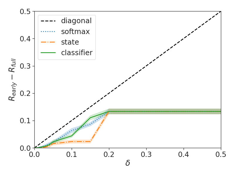
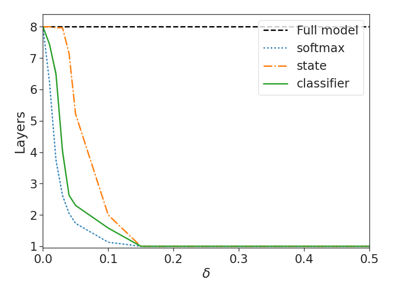
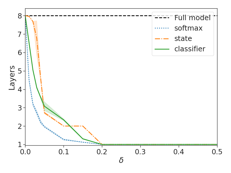
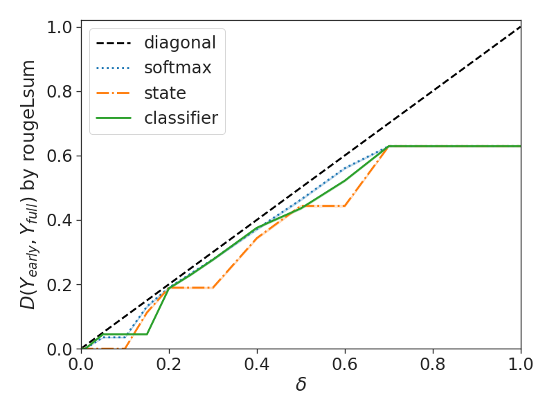
Next, we examine the outcomes of the calibration process. Since the obtained risk is guaranteed to be valid (i.e., $\leq\delta$ at least 95% of the time), we focus here on efficiency gains per chosen $\delta$. We refer the reader to Appendix B for empirical validation and for additional results and qualitative examples.

Table 2 presents the efficiency gains per choice of $\delta$ for each consistency objective and confidence measure. We examine larger $\delta$ values for textual consistency as this is generally a stricter requirement since the full model’s error is not considered.

Across all, the softmax confidence measure leads to the greatest decrease in number of decoder layers required. Accordingly, softmax mostly enables the highest speedup gains of up to about three times faster than running through all the model’s layers. The very lightweight early-exit classifier sometimes provides better gains than softmax, even if more decoding layers are used. Since the speedup is computed over the full generated output, we see more gains on the longer outputs of summarization and translation where the decoding takes most of the time, compared to the short QA outputs where the whole decoding time is not much longer than the encoding time.

These encouraging efficiency gains are enabled even with the rigorous performance guarantees that are sometimes conservative (e.g., Eq. (11)). We note that relaxing these constraints, or tightening the confidence intervals (e.g., with larger calibration sets), can further improve the empirical gains.

The softmax operation over the full output vocabulary is FLOPs heavy (though, this compute can potentially be paralleled), sometime leading to increased total FLOPs, even with fewer used layers. The state-based and early-exit classifier measures require minimal FLOPs and provide a good alternative with compelling efficiency gains, if total (parallizeable, or not) FLOPs is of concern.

6.2 Example output: effectively distributing the model’s capacity across timesteps

Figure 4 presents two CALM summary generations for an article from the CNN/DM dataset, compared to the output of the full model (See Figure B.5 in the Appendix for examples from the other tasks). $Y^{(2)}_{\mathrm{early}}$ uses a lower confidence threshold for early exiting compared to $Y^{(1)}_{\mathrm{early}}$. The colors, depicting the number of decoder layers used per output token, illustrate how CALM obtains the efficiency gains. Only a few selected tokens use the full capacity of the model (colored in red), while for most tokens the model exits after one or few decoding layers (colored in green).

The example in Figure 4 also demonstrates one difference between the two types of consistency constraints, given a reference output $Z_{\mathrm{test}}$. Textual consistency $D(Y_{\mathrm{early}},Y_{\mathrm{full}})$ generally (though, not always) degrades (i.e., increases) when decreasing the confidence threshold as the outputs tend to more significantly diverge from $Y_{\mathrm{full}}$. The trend of risk consistency, however, depends also on the reference output $Z_{\mathrm{test}}$. If $Y_{\mathrm{full}}\approx Z_{\mathrm{test}}$ then the two constraints are nearly the same. In this example, they are sufficiently different that $Y^{(2)}_{\mathrm{early}}$ obtained better (lower) risk even though the textual distance from $Y_{\mathrm{full}}$ is higher. On the one hand, given the availability of reference outputs for calibration, this suggests that for an imperfect model, risk consistency could lead to more aggressive early-exiting while maintaining the quality of generations. On the other hand, since the $\mathop{Relu}$ in Eq. (11) doesn’t reward negative risk differences, the benefits might not fully materialize. Overall, the two constraints provide different alternatives for the user to choose from depending on the availability of reference outputs, the performance of the full model, and the exact desired performance guarantees.

Figure 4: CALM accelerates the generation by early exiting when possible, and selectively using the full decoder’s capacity only for few tokens, demonstrated here on a CNN/DM example with softmax-based confidence measure. $Y^{(1)}_{\mathrm{early}}$ and $Y^{(2)}_{\mathrm{early}}$ use different confidence thresholds for early exiting. Bellow the text, we report the measured textual and risk consistency of each of the two outputs, along with efficiency gains. The colors represent the number of decoding layers used for each token—light green shades indicate less than half of the total layers.

7 Conclusion

We present confident adaptive language modeling (CALM) for dynamically allocating different amounts of compute per generated token, following explicitly defined tolerance levels on the full generation output. This paper covers both modeling solutions and analyses towards this goal, as well as a theoretically-grounded framework for provably controlling the quality of the full output to meet the user-specified tolerance levels. We investigate the effects of local early exiting during decoding on the final output, leading us to propose a decaying function over the initial threshold that enables finer control over the performance-efficiency tradeoffs without inflating the search space. We also study different solutions for addressing missing computations of early-exited tokens that are dependent upon for future tokens. Overall, our complete adaptive compute framework for LMs requires minimal modifications to the underlying model and enables efficiency gains while satisfying rigorous quality guarantees for the output. Also, our oracle experiments and runtime analysis demonstrates the full potential of this framework and leave room for future research to further improve the efficiency in a controllable way.

Appendix A Mathematical Details

A.1 Proof of Proposition 1

Proof.

Define $\lambda$ to be risk-controlling if $\mathrm{LLM}_{\mathrm{early}}(P_{\mathrm{test}},{\lambda})$ $\mathrm{LLM}_{\mathrm{full}}(P_{\mathrm{test}})$ are consistent. Suppose $\Lambda_{\mathrm{valid}}$ is non-empty. Then all $\lambda\in\Lambda_{\mathrm{valid}}$ are risk-controlling w.p. $\geq 1-\epsilon$, per Thm. 1 of Angelopoulos et al. [2021]. Furthermore, per Eq. (4) for $\lambda=1$ we have $\mathrm{LLM_{early}}(P_{\mathrm{test}},1)=\mathrm{LLM}_{\mathrm{full}}(P_{\mathrm{test}})$ by definition, since $\sup\mathcal{M}_{i}(h_{i})=1$, $\forall i\in[1,\ldots,L]$. Thus $\lambda=1$ is also risk-controlling by definition. Combined, all $\lambda\in\Lambda_{\mathrm{valid}}\cup\{1\}$ are risk-controlling w.p. $\geq 1-\epsilon$, and therefore $\lambda:=\min(\Lambda_{\mathrm{valid}}\cup\{1\})$ is always well-defined and guaranteed to be risk-controlling w.p. $\geq 1-\epsilon$. ∎

Appendix B Additional Results

We provide additional experimental results to supplement Section 6. In Section B.1, we include calibration plots, for both the validation and test sets, with the full range of $\delta$, also showing the standard deviation across random trials. In Section B.2, we present a few example outputs with a visualization of the per-token early-exit decisions to illustrate CALM’s behavior. In Section B.3, we include results of a larger 12-layer model, showing the generalizability of our framework to other configurations.

B.1 Calibration results for the full tolerance range

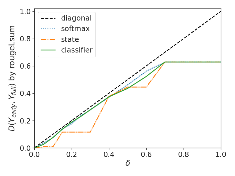
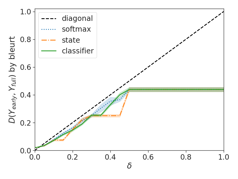
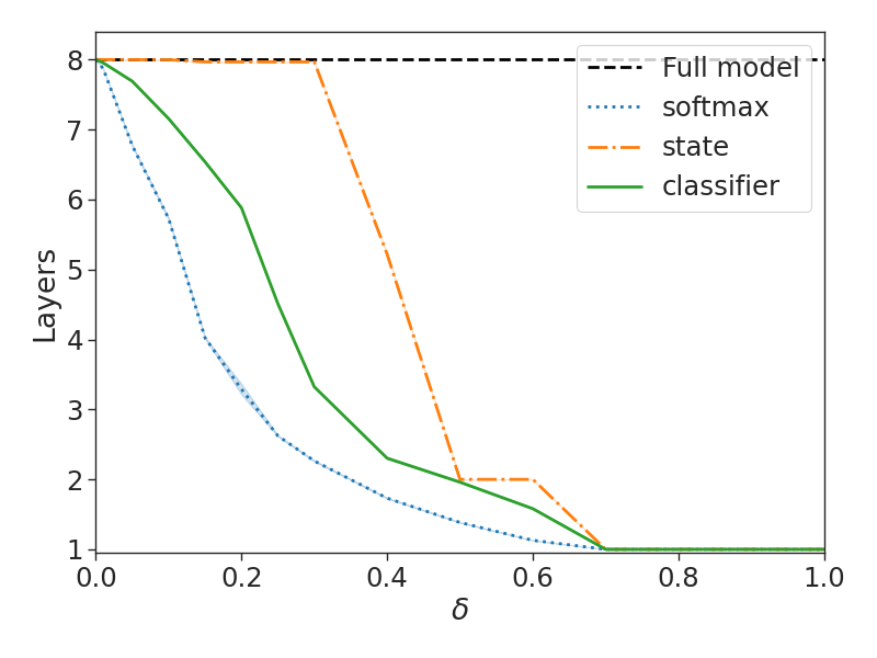
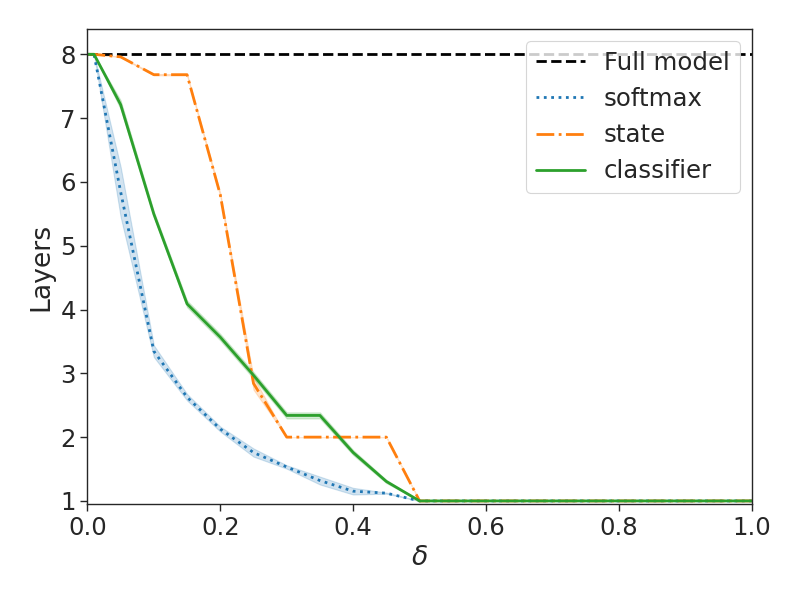
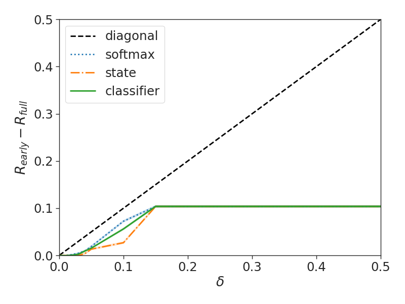
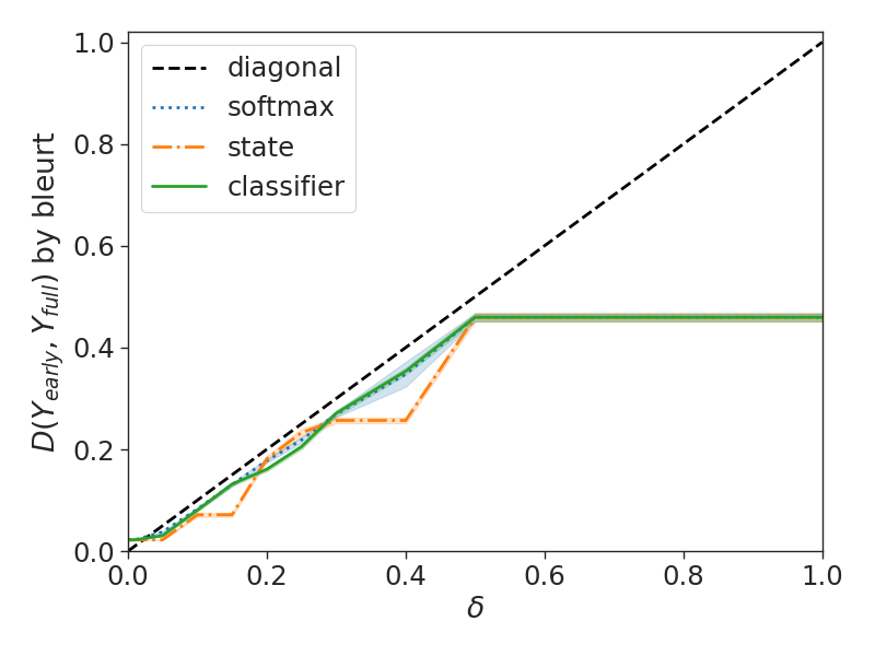
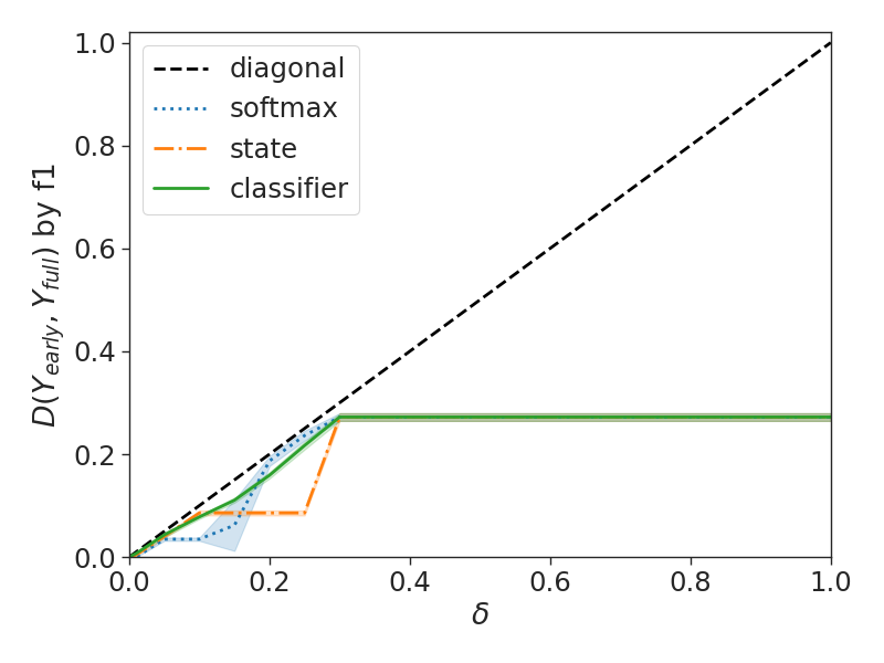
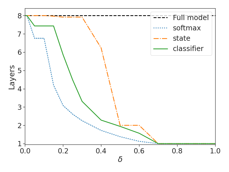
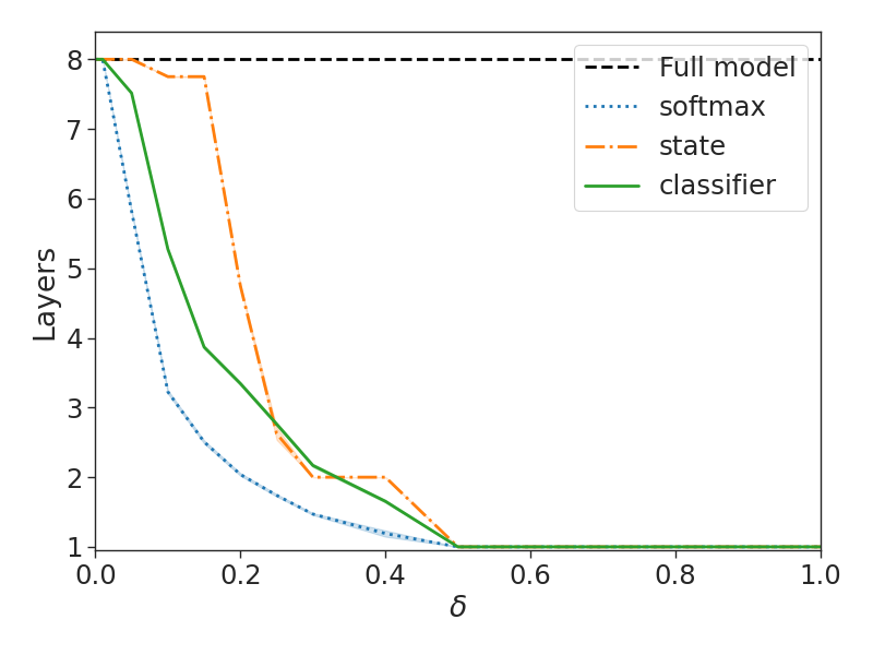
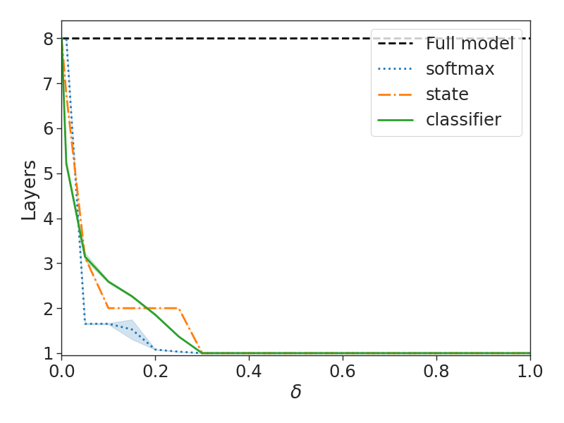
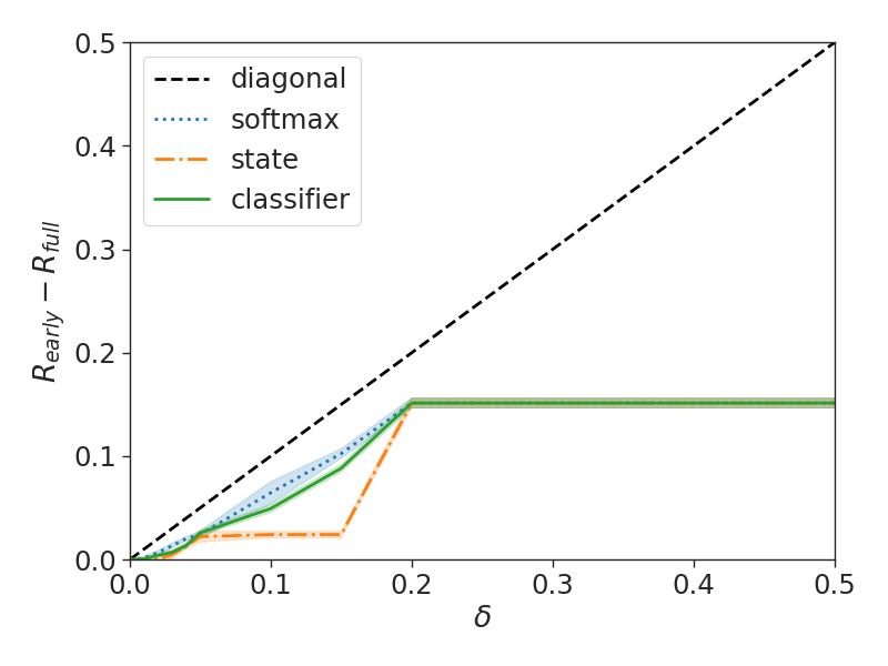
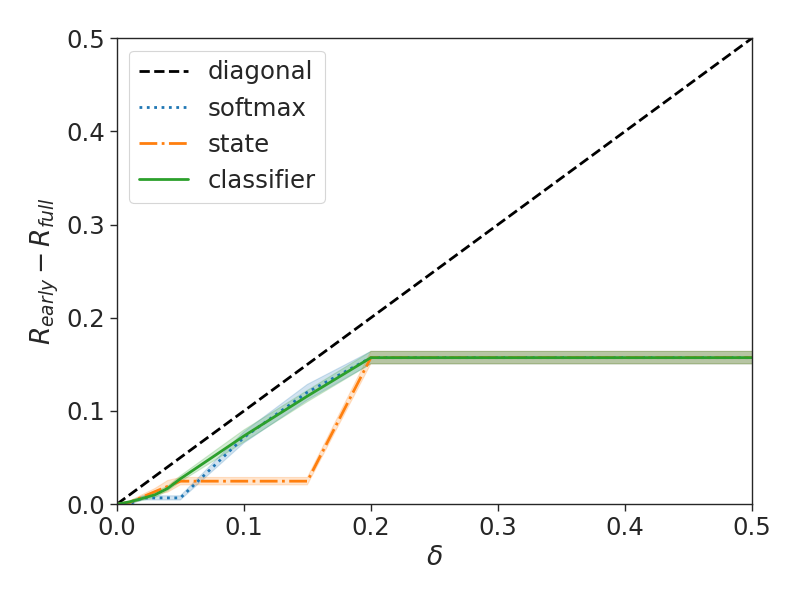
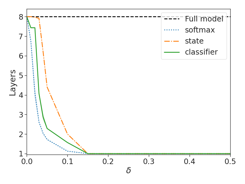
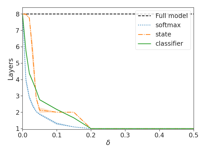
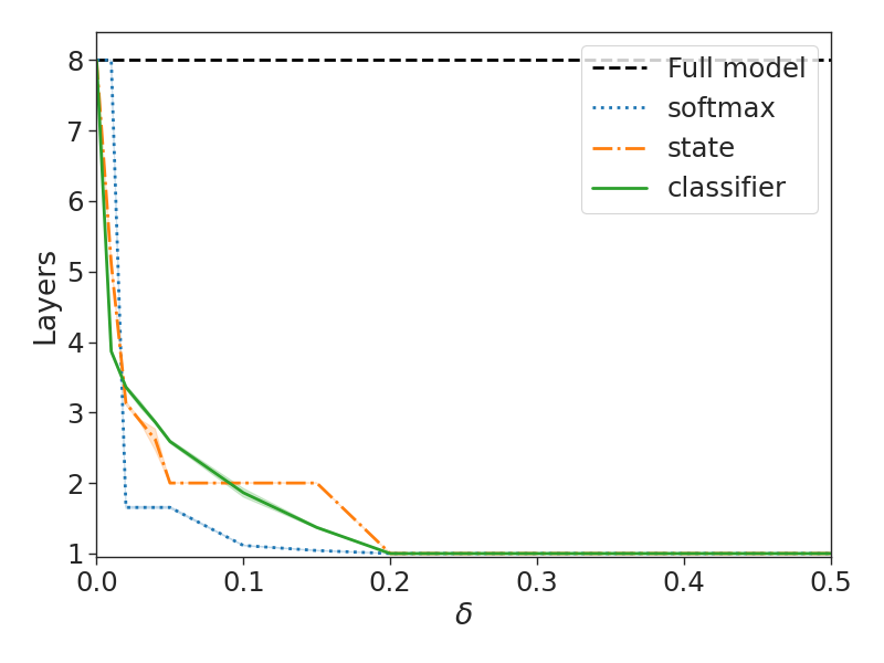
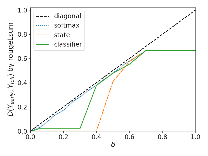
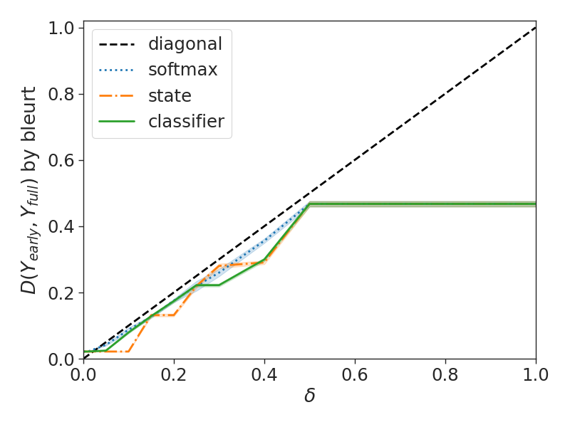
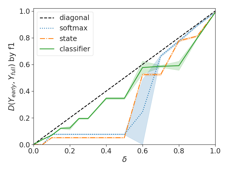
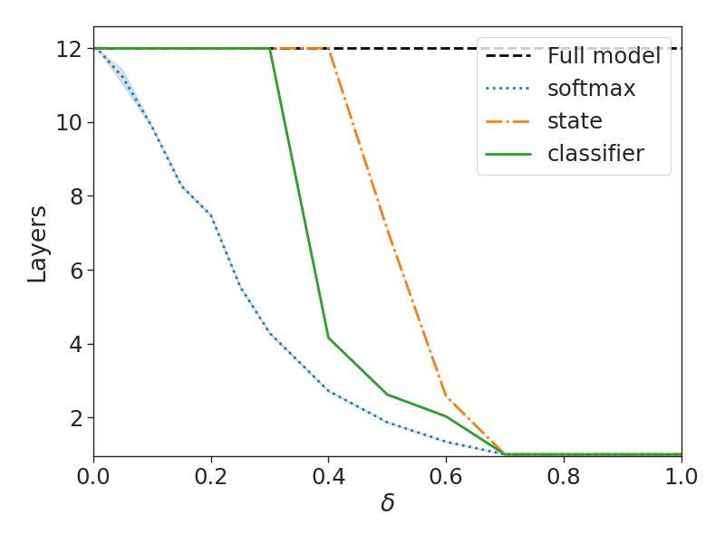
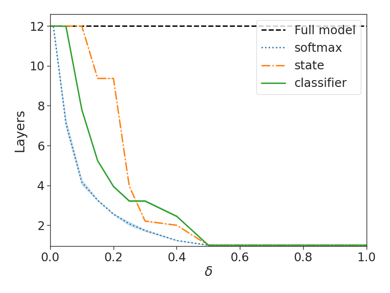
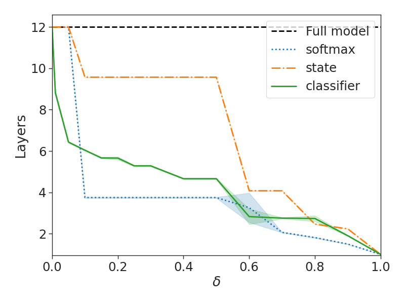
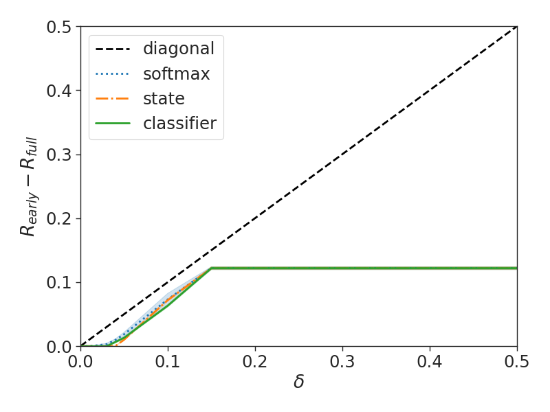
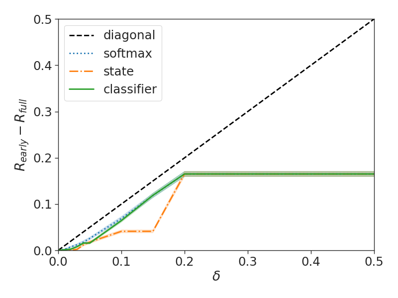
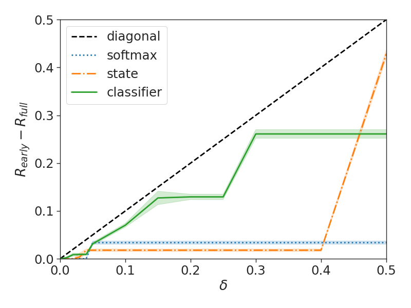
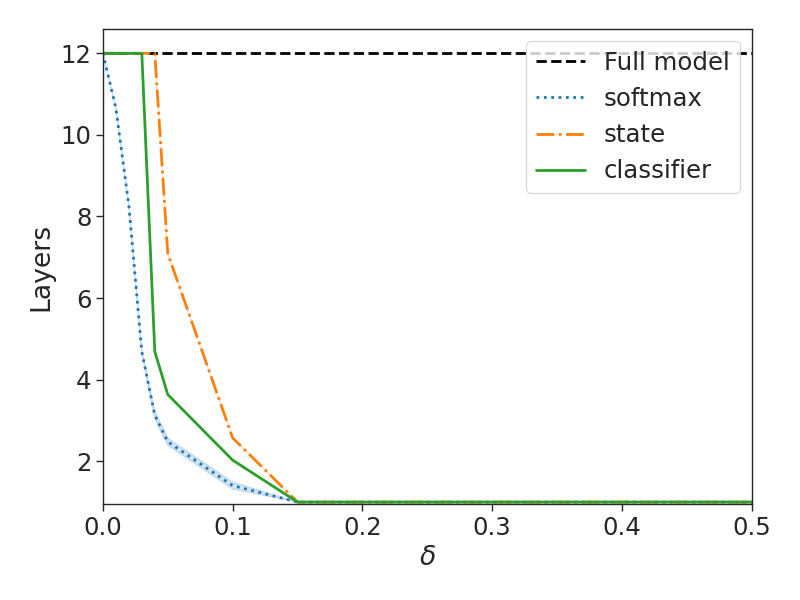
We present complementary results to Table 2. Figure B.1 and Figure B.2 present the empirical consistencies and efficiency gains for textual and risk consistency constraints, respectively. Figure B.3 and Figure B.4 report the same on the validation datasets. First, we observe that the calibration holds empirically, achieving risk values that are not greater than the specified $\delta$ (i.e., being under the diagonal in the upper subplots). We also see that the risk is often lower than allowed for (a good thing), especially with the risk consistency objective. This is due to the conservativeness of our measure (Eq. (11)), not rewarding instances where the early prediction has lower risk. While obtaining lower risk than the target is not a downside, this indicates that there is further potential in improving the efficiency gains achieved per $\delta$. Yet, even with the rigorous and conservative theoretical guarantees, we already obtain significant efficiency gains that, naturally, increase with larger tolerance values.

(a) CNN/DM

(b) WMT

Figure B.1: Textual consistency and efficiency gains over the test sets per choice of $\delta$ ($\epsilon=0.05$). The top row presents the empirical consistency where being under the diagonal means satisfying $\delta$ consistency. The bottom row presents the average number of decoder layer used. Shaded areas represent the standard deviation over random trials.

(a) CNN/DM

(b) WMT

Figure B.2: Risk consistency and efficiency gains over the test sets per choice of $\delta$ ($\epsilon=0.05$). The top row presents the empirical consistency where being under the diagonal means satisfying $\delta$ consistency. The bottom row presents the average number of decoder layer used. Shaded areas represent the standard deviation over random trials.

(a) CNN/DM

(b) WMT

(c) SQuAD

Figure B.3: Textual consistency and efficiency gains over the validation sets per choice of $\delta$ ($\epsilon=0.05$). The top row presents the empirical consistency where being under the diagonal means satisfying $\delta$ consistency. The bottom row presents the average number of decoder layer used. Shaded areas represent the standard deviation over random trials.

(a) CNN/DM

(b) WMT

(c) SQuAD

Figure B.4: Risk consistency and efficiency gains over the validation sets per choice of $\delta$ ($\epsilon=0.05$). The top row presents the empirical consistency where being under the diagonal means satisfying $\delta$ consistency. The bottom row presents the average number of decoder layer used. Shaded areas represent the standard deviation over random trials.

B.2 Qualitative examples

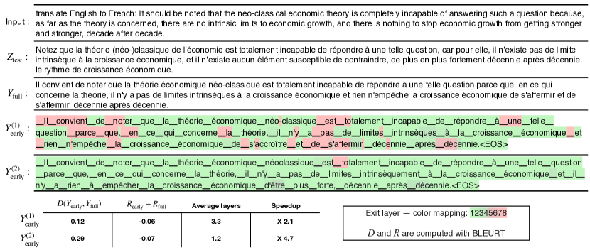
Figure B.5 presents two example outputs of CALM for instances from the machine translation, and question-answering (QA) datasets (See Figure 4 for summarization). The colors depict the per-token number of decoder layers that were used for generating that output. We also report the risk values for textual and risk consistency of both outputs, as well as the speedup compared to the full model. We observe that the textual distance generally increases as we accelerate the decoding. Though, the outputs still remain relatively similar to the full model even when using very few layers. The risk consistency doesn’t always correlate with the textual one when the full model’s risk is non-zero. In some cases, the accelerated output has even lower risk than the full model’s output. This demonstrates the value of having both our textual and risk consistency configurations, which the user can pick from based on their objective, and whether quality reference outputs for calibration are available or not.

Interestingly, following our initial intuition, CALM distributes the compute unevenly, using very few layers for certain “easy” tokens, and additional compute to “hard” tokens. Examining the examples, we see that many times “hard” generation steps come at the beginning of sentences, or when generating a verb. We leave further investigations on perceived difficulties to future work.

(a) WMT EN-FR

(b) SQuAD

Figure B.5: Example outputs of CALM using a softmax-based confidence measure. Bellow the text, we report the measured textual and risk consistency of each of the two outputs, along with efficiency gains. See Figure 4 for an example from the CNN/DM task.

B.3 T5-base results

While throughout the rest of this paper we experiment with a 8-layer encoder-decoder T5 model. We include here results for a 12-layer T5-base model that besides the additional layers is also larger in its internal dimensions, having 12 attention heads and 64, 768, and 2048 dimensions for the attention head, embeddings, and MLP, respectively.

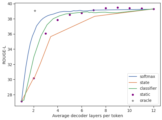
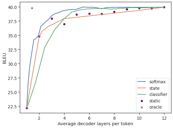
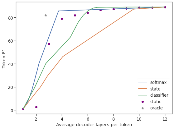
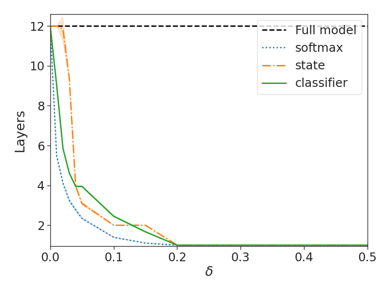
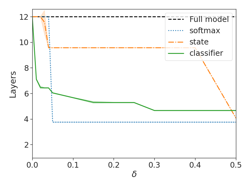
Figure B.6 shows the empirical performance-efficiency tradeoffs achieved with this model on the three tasks. Overall, we the trends are very similar to the one observed with the 8-layer model (Figure 3). One exception is the SQuAD model where the static baseline that uses only one or two decoder layers completely fails. This suggests that the actual predictions of this model are starting to be formed only from the third layer. Also, the local oracle measure on SQuAD obtains slightly lower global performance compared to the full model, also suggesting that in this case the hidden-state of the very low layers might not be a good enough representation for followup generations. Yet, the softmax and early-exit classifier confidence measure provide good proxies for the consistency and often outperform the static baselines. In the other two datasets, the local oracle matches the performance of the full model, similar to the behavior of the 8-layer model.

Figure B.7 and Figure B.8 present the validity and efficiency gains of our calibration procedure on the 12-layer model for textual and risk consistency objectives, respectively. We observe a largely similar behavior as the 8-layer model, showing the generality of our framework to other configurations of the backbone language model.

(a) CNN/DM

(b) WMT

(c) SQuAD

Figure B.6: T5-base (12 layers) validation empirical performance-efficiency tradeoffs for different confidence measures, compared to static baselines and a local oracle measure.

(a) CNN/DM

(b) WMT

(c) SQuAD

Figure B.7: Textual consistency and efficiency gains with a 12-layer T5-base model over the validation sets per choice of $\delta$ ($\epsilon=0.05$). The top row presents the empirical consistency where being under the diagonal means satisfying $\delta$ consistency. The bottom row presents the average number of decoder layer used. Shaded areas represent the standard deviation over random trials.

(a) CNN/DM

(b) WMT

(c) SQuAD

Figure B.8: Risk consistency and efficiency gains with a 12-layer T5-base model over the validation sets per choice of $\delta$ ($\epsilon=0.05$). The top row presents the empirical consistency where being under the diagonal means satisfying $\delta$ consistency. The bottom row presents the average number of decoder layer used. Shaded areas represent the standard deviation over random trials.

Appendix C Implementation Details

As mentioned in Section 5, we build on the T5 encoder-decoder model [Raffel et al., 2019], and us the T5X repository [Roberts et al., 2022] for implementing CALM. Appendix E describes the main algorithmic components.

Our main experiments use the T5 1.1 version with 8 layers for both the encoder and decoder modules, 6 attention heads with dimensions of 64, 512, and 1024 for the attention head, embeddings, and MLP, respectively. The vocabulary contains 32,128 tokens. This model doesn’t share the input and output embeddings. For our early-exit head, we share the output embeddings between all intermediate with the top one, not introducing any new parameters to the model. Our binary early-exit classifier is also shared across all layers, adding only a very small amount of new parameters. We add early-exit heads to all layers.

We fine-tune the models on the training set of each task for a maximum of 500K steps, and choose the best checkpoint by performance on the validation set (using the full models’ predictions). We use a batch size of 128, the regular LM cross-entropy loss, the AdaFactor optimizer [Shazeer and Stern, 2018], and experiment with learning rates $10^{-3}$ and $10^{-4}$. We aggregate the loss of individual layers with a weighted average, as discussed in Section 3.4. For the early-exit classifier training, we use an unweighted average (See Appendix D for more details). We use 64 TPUv3 chips for training. For inference, we use a single TPUv4 chip with a batch size of one, simulating a one-at-a-time processing setting, that is convenient when serving models for online requests. As described in Section 3.2, CALM exits early whenever the per-token confidence value $c$ (Section 3.5) exceeds the possibly-decaying threshold $\lambda$ (Section 3.3.2) derived from the user-defined $\delta,\epsilon$ tolerance levels and textual or risk consistency objective (Section 4). If necessary, the hidden-state is propagated to the skipped layers (Section 3.3.1).

C.1 FLOPs and speedup computations

We detail our procedures for approximating the reference efficiency gains using the FLOPs and speedup measures. For FLOPs computation, to be consistent with Elbayad et al. [2020] (See their Appendix B), we adopt their formula to compute the average decoder FLOPs per output token.

To measure the speedup of early exiting with CALM, we execute 200 inference predictions for each task under each examined configuration in a JIT compiled function in colab with TPUv3. We ignore the time of the first execution, since it is drastically slower due to compilation, and average the rest of the measured times. For each inference prediction, we use batch size one, and measure the full generation time including both the encoder and all decoding steps until completion. For each examined confidence measure (softmax, state, or classifier), we compute the speedup by comparing to the average inference time of the full model that uses all layers, by setting the confidence threshold to maximum. We note that our implementation adds conditionals between layers that add some overhead to the compute graph. Yet, even compared to a conditional-free implementation, the gains of CALM’s early exits often outweigh the overheads of the added conditionals. We leave studying further technical improvements to the implementation to future work.

Appendix D Training Details of the Early Exit Classifier

Table D.1: $F_{1}$ scores of early-exit classifier for predicting not to exit. Measured at layers 1,4, and 7.

	CNN/DM			WMT			SQuAD
Training method	$i=1$	4	7	$i=1$	4	7	$i=1$	4	7
Geometric-like	.59	.35	.24	.33	.18	.11	.73	.16	.11
Independent	.62	.49	.37	.51	.34	.24	.76	.26	.18

As discussed in Section 3.5, we train the early exit classifier to predict whether the top-ranked prediction of a specific intermediate layer is the same as the prediction of the top layer. This classifier is using the intermediate hidden-state as its input features. The target labels are computed on-the-fly following an oracle that compares the intermediate prediction head with the prediction of the full model ($\mathbbm{1}[\operatorname*{arg\,max}(p(y_{t+1}|d_{t}^{i})=\operatorname*{arg\,max}(p(y_{t+1}|d_{t}^{L})]$). We use the same training hyper-parameters used for the full model, but freeze all parameters of the backbone model (to eliminate any affect on the model’s performance) and only train the newly added parameters for early-exit classifier, which are shared across all layers.

Following the setup above, we compute the binary cross-entropy loss for each layer individually, and aggregate by taking the unweighted average across all layers. We use the loss value on the validation set to pick the best checkpoint. We also explore with the geometric-like objective proposed by Elbayad et al. [2020]. Their approach views the exiting decisions as a Bernoulli process, using the “exit”/ “don’t exit” predicted probabilities. The goal is to make an “exit” prediction at the first true layer, determined by the oracle, and “don’t exit” predictions by all preceding layers. Accordingly, the training objective maximizes the probability of this oracle-guided event, modeled as a product of all respective predicted probabilities. In practice, due to numerical instability of this product operation, we maximize the summation over the log probabilities.

Table D.1 presents the $F_{1}$ validation scores of “don’t exit” predictions (with a $0.5$ threshold) by early-exit classifier, measured against the oracle for layers 1,4, and 7. Our per-layer independent training objective outperforms the geometric-like objective across all layers and tasks. The advantage is typically most pronounced for higher layers. We conjecture that this is due to the equal weight of the independent objective that utilizes signal from all layers, whereas the geometric-like objective only learns from layers up to the first oracle exit.

Appendix E Algorithms and Code

Algorithm 1 Calibrating CALM for global consistency within $\delta,\epsilon$ tolerance levels with FST-based LTT Angelopoulos et al. [2021].

1:function calibrate($\text{LLM}_{\mathrm{early}},\text{LLM}_{\mathrm{full}},\delta,\epsilon$)

2:    $\lambda_{\mathrm{min}}=1$

3:    $\Lambda=(\lambda_{1},\lambda_{2},\ldots,\lambda_{k})$$\triangleright$ Arrange decreasing candidate thresholds, $\lambda_{i}>\lambda_{j}$ $\forall i<j$.

4:    for $\lambda_{j}\in\Lambda$ do

5:         $\widehat{E}(\lambda_{j})=\frac{1}{n}\sum_{i=1}^{n}L_{i}(\lambda_{j})$ $\triangleright$ Following Eqs. (10) or (11) for textual vs. risk consistency.

6:         $p_{j}=\exp(-2n(\max(0,\delta-\widehat{E}(\lambda_{j})))^{2})$ $\triangleright$ Compute p-value. Can replace with Hoeffding-Bentkus.

7:         if $p_{j}>\epsilon$ then

8:             return $\lambda_{\mathrm{min}}$          

9:         $\lambda_{\mathrm{min}}=\lambda_{j}$     

10:    return $\lambda_{\mathrm{min}}$

Algorithm 1 describes the calibration process of CALM for obtaining global textual or risk $\delta,\epsilon$ consistency (Section 4).

The JAX [Bradbury et al., 2018] code for training CALM models and for executing the early-exit functionality at inference-time is available at: https://github.com/google-research/t5x/tree/main/t5x/contrib/calm

References

- Angelopoulos and Bates [2021a] Anastasios N. Angelopoulos and Stephen Bates. A gentle introduction to conformal prediction and distribution-free uncertainty quantification. 2021a. doi: 10.48550/ARXIV.2107.07511. URL https://arxiv.org/abs/2107.07511.
- Angelopoulos and Bates [2021b] Anastasios Nikolas Angelopoulos and Stephen Bates. A gentle introduction to conformal prediction and distribution-free uncertainty quantification, 2021b. URL https://arxiv.org/abs/2107.07511.
- Angelopoulos et al. [2021] Anastasios Nikolas Angelopoulos, Stephen Bates, Emmanuel J. Candès, Michael I. Jordan, and Lihua Lei. Learn then test: Calibrating predictive algorithms to achieve risk control. ArXiv preprint: 2110.01052, 2021.
- Angelopoulos et al. [2022] Anastasios Nikolas Angelopoulos, Amit Kohli, Stephen Bates, Michael I. Jordan, Jitendra Malik, Thayer Alshaabi, Srigokul Upadhyayula, and Yaniv Romano. Image-to-image regression with distribution-free uncertainty quantification and applications in imaging. ArXiv, abs/2202.05265, 2022.
- Aribandi et al. [2022] Vamsi Aribandi, Yi Tay, Tal Schuster, Jinfeng Rao, Huaixiu Steven Zheng, Sanket Vaibhav Mehta, Honglei Zhuang, Vinh Q. Tran, Dara Bahri, Jianmo Ni, Jai Gupta, Kai Hui, Sebastian Ruder, and Donald Metzler. Ext5: Towards extreme multi-task scaling for transfer learning. In International Conference on Learning Representations, 2022. URL https://openreview.net/forum?id=Vzh1BFUCiIX.
- Bai et al. [2020] Haoli Bai, Wei Zhang, Lu Hou, Lifeng Shang, Jing Jin, Xin Jiang, Qun Liu, Michael Lyu, and Irwin King. Binarybert: Pushing the limit of bert quantization. arXiv preprint arXiv:2012.15701, 2020.
- Bai et al. [2022] Yu Bai, Song Mei, Haiquan Wang, Yingbo Zhou, and Caiming Xiong. Efficient and differentiable conformal prediction with general function classes. ArXiv, abs/2202.11091, 2022.
- Baier-Reinio and Sterck [2020] Aaron Baier-Reinio and Hans De Sterck. N-ode transformer: A depth-adaptive variant of the transformer using neural ordinary differential equations. ArXiv, abs/2010.11358, 2020.
- Bapna et al. [2020] Ankur Bapna, Naveen Arivazhagan, and Orhan Firat. Controlling computation versus quality for neural sequence models. 2020. doi: 10.48550/ARXIV.2002.07106. URL https://arxiv.org/abs/2002.07106.
- Bates et al. [2020] Stephen Bates, Anastasios Nikolas Angelopoulos, Lihua Lei, Jitendra Malik, and Michael I. Jordan. Distribution free, risk controlling prediction sets. ArXiv preprint: 2101.02703, 2020.
- Bauer [1991] Peter Bauer. Multiple testing in clinical trials. Statistics in medicine, 10 6:871–89; discussion 889–90, 1991.
- Bentkus [2004] Vidmantas Bentkus. On hoeffding’s inequalities. Annals of Probability, 32:1650–1673, 2004.
- Bojar et al. [2015] Ondřej Bojar, Rajen Chatterjee, Christian Federmann, Barry Haddow, Matthias Huck, Chris Hokamp, Philipp Koehn, Varvara Logacheva, Christof Monz, Matteo Negri, Matt Post, Carolina Scarton, Lucia Specia, and Marco Turchi. Findings of the 2015 workshop on statistical machine translation. In Proceedings of the Tenth Workshop on Statistical Machine Translation, pages 1–46, Lisbon, Portugal, September 2015. Association for Computational Linguistics. doi: 10.18653/v1/W15-3001. URL https://aclanthology.org/W15-3001.
- Bradbury et al. [2018] James Bradbury, Roy Frostig, Peter Hawkins, Matthew James Johnson, Chris Leary, Dougal Maclaurin, George Necula, Adam Paszke, Jake VanderPlas, Skye Wanderman-Milne, and Qiao Zhang. JAX: composable transformations of Python+NumPy programs, 2018. URL http://github.com/google/jax.
- Brown et al. [2020] Tom Brown, Benjamin Mann, Nick Ryder, Melanie Subbiah, Jared D Kaplan, Prafulla Dhariwal, Arvind Neelakantan, Pranav Shyam, Girish Sastry, Amanda Askell, Sandhini Agarwal, Ariel Herbert-Voss, Gretchen Krueger, Tom Henighan, Rewon Child, Aditya Ramesh, Daniel Ziegler, Jeffrey Wu, Clemens Winter, Chris Hesse, Mark Chen, Eric Sigler, Mateusz Litwin, Scott Gray, Benjamin Chess, Jack Clark, Christopher Berner, Sam McCandlish, Alec Radford, Ilya Sutskever, and Dario Amodei. Language models are few-shot learners. In H. Larochelle, M. Ranzato, R. Hadsell, M.F. Balcan, and H. Lin, editors, Advances in Neural Information Processing Systems, volume 33, pages 1877–1901. Curran Associates, Inc., 2020. URL https://proceedings.neurips.cc/paper/2020/file/1457c0d6bfcb4967418bfb8ac142f64a-Paper.pdf.
- Cambazoglu et al. [2010] Berkant Barla Cambazoglu, Hugo Zaragoza, Olivier Chapelle, Jiang Chen, Ciya Liao, Zhaohui Zheng, and Jon Degenhardt. Early exit optimizations for additive machine learned ranking systems. In WSDM ’10, 2010.
- Chowdhery et al. [2022] Aakanksha Chowdhery, Sharan Narang, Jacob Devlin, Maarten Bosma, Gaurav Mishra, Adam Roberts, Paul Barham, Hyung Won Chung, Charles Sutton, Sebastian Gehrmann, Parker Schuh, Kensen Shi, Sasha Tsvyashchenko, Joshua Maynez, Abhishek Rao, Parker Barnes, Yi Tay, Noam Shazeer, Vinodkumar Prabhakaran, Emily Reif, Nan Du, Ben Hutchinson, Reiner Pope, James Bradbury, Jacob Austin, Michael Isard, Guy Gur-Ari, Pengcheng Yin, Toju Duke, Anselm Levskaya, Sanjay Ghemawat, Sunipa Dev, Henryk Michalewski, Xavier Garcia, Vedant Misra, Kevin Robinson, Liam Fedus, Denny Zhou, Daphne Ippolito, David Luan, Hyeontaek Lim, Barret Zoph, Alexander Spiridonov, Ryan Sepassi, David Dohan, Shivani Agrawal, Mark Omernick, Andrew M. Dai, Thanumalayan Sankaranarayana Pillai, Marie Pellat, Aitor Lewkowycz, Erica Moreira, Rewon Child, Oleksandr Polozov, Katherine Lee, Zongwei Zhou, Xuezhi Wang, Brennan Saeta, Mark Diaz, Orhan Firat, Michele Catasta, Jason Wei, Kathy Meier-Hellstern, Douglas Eck, Jeff Dean, Slav Petrov, and Noah Fiedel. Palm: Scaling language modeling with pathways. 2022.
- Dehghani et al. [2019] Mostafa Dehghani, Stephan Gouws, Oriol Vinyals, Jakob Uszkoreit, and Lukasz Kaiser. Universal transformers. In International Conference on Learning Representations (ICLR), 2019.
- Dehghani et al. [2022] Mostafa Dehghani, Yi Tay, Anurag Arnab, Lucas Beyer, and Ashish Vaswani. The efficiency misnomer. In International Conference on Learning Representations, 2022. URL https://openreview.net/forum?id=iulEMLYh1uR.
- Devlin et al. [2019] Jacob Devlin, Ming-Wei Chang, Kenton Lee, and Kristina Toutanova. BERT: Pre-training of deep bidirectional transformers for language understanding. In Proceedings of the 2019 Conference of the North American Chapter of the Association for Computational Linguistics: Human Language Technologies, Volume 1 (Long and Short Papers), pages 4171–4186, Minneapolis, Minnesota, June 2019. Association for Computational Linguistics. doi: 10.18653/v1/N19-1423. URL https://aclanthology.org/N19-1423.
- Dey et al. [2021] Neil Dey, Jing Ding, Jack G. Ferrell, Carolina Kapper, Maxwell Lovig, Emiliano Planchon, and Jonathan P Williams. Conformal prediction for text infilling and part-of-speech prediction. ArXiv, abs/2111.02592, 2021.
- Du et al. [2021] Nan Du, Yanping Huang, Andrew M. Dai, Simon Tong, Dmitry Lepikhin, Yuanzhong Xu, Maxim Krikun, Yanqi Zhou, Adams Wei Yu, Orhan Firat, Barret Zoph, Liam Fedus, Maarten Bosma, Zongwei Zhou, Tao Wang, Yu Emma Wang, Kellie Webster, Marie Pellat, Kevin Robinson, Kathy Meier-Hellstern, Toju Duke, Lucas Dixon, Kun Zhang, Quoc V Le, Yonghui Wu, Zhifeng Chen, and Claire Cui. Glam: Efficient scaling of language models with mixture-of-experts. 2021.
- Elbayad et al. [2020] Maha Elbayad, Jiatao Gu, Edouard Grave, and Michael Auli. Depth-adaptive transformer. In International Conference on Learning Representations, 2020. URL https://openreview.net/forum?id=SJg7KhVKPH.
- Fan et al. [2019] Angela Fan, Edouard Grave, and Armand Joulin. Reducing transformer depth on demand with structured dropout. arXiv preprint arXiv:1909.11556, 2019.
- Figurnov et al. [2017] Michael Figurnov, Artem Sobolev, and Dmitry P. Vetrov. Probabilistic adaptive computation time. ArXiv, abs/1712.00386, 2017.
- Fisch et al. [2021] Adam Fisch, Tal Schuster, Tommi Jaakkola, and Regina Barzilay. Efficient conformal prediction via cascaded inference with expanded admission. In International Conference on Learning Representations (ICLR), 2021.
- Fisch et al. [2022] Adam Fisch, Tal Schuster, T. Jaakkola, and Regina Barzilay. Conformal prediction sets with limited false positives. ArXiv, abs/2202.07650, 2022.
- Geva et al. [2022] Mor Geva, Avi Caciularu, Kevin Ro Wang, and Yoav Goldberg. Transformer feed-forward layers build predictions by promoting concepts in the vocabulary space. 2022.
- Graves [2016] Alex Graves. Adaptive computation time for recurrent neural networks. 2016.
- Gulcehre et al. [2017] Caglar Gulcehre, Orhan Firat, Kelvin Xu, Kyunghyun Cho, and Yoshua Bengio. On integrating a language model into neural machine translation. Computer Speech & Language, 45:137–148, 2017. ISSN 0885-2308. doi: https://doi.org/10.1016/j.csl.2017.01.014. URL https://www.sciencedirect.com/science/article/pii/S0885230816301395.
- Hermann et al. [2015] Karl Moritz Hermann, Tomas Kocisky, Edward Grefenstette, Lasse Espeholt, Will Kay, Mustafa Suleyman, and Phil Blunsom. Teaching machines to read and comprehend. In C. Cortes, N. Lawrence, D. Lee, M. Sugiyama, and R. Garnett, editors, Advances in Neural Information Processing Systems, volume 28. Curran Associates, Inc., 2015. URL https://proceedings.neurips.cc/paper/2015/file/afdec7005cc9f14302cd0474fd0f3c96-Paper.pdf.
- Hinton et al. [2015] Geoffrey E. Hinton, Oriol Vinyals, and Jeffrey Dean. Distilling the knowledge in a neural network. ArXiv, abs/1503.02531, 2015.
- Hoeffding [1963] Wassily Hoeffding. Probability inequalities for sums of bounded random variables. Journal of the American Statistical Association, 58:13–30, 1963.
- Hou et al. [2020] Lu Hou, Zhiqi Huang, Lifeng Shang, Xin Jiang, Xiao Chen, and Qun Liu. Dynabert: Dynamic bert with adaptive width and depth. Advances in Neural Information Processing Systems, 33:9782–9793, 2020.
- Jernite et al. [2016] Yacine Jernite, Edouard Grave, Armand Joulin, and Tomas Mikolov. Variable computation in recurrent neural networks. arXiv preprint arXiv:1611.06188, 2016.
- Jiao et al. [2019] Xiaoqi Jiao, Yichun Yin, Lifeng Shang, Xin Jiang, Xiao Chen, Linlin Li, Fang Wang, and Qun Liu. Tinybert: Distilling bert for natural language understanding. arXiv preprint arXiv:1909.10351, 2019.
- Kasai et al. [2021] Jungo Kasai, Nikolaos Pappas, Hao Peng, James Cross, and Noah Smith. Deep encoder, shallow decoder: Reevaluating non-autoregressive machine translation. In International Conference on Learning Representations, 2021. URL https://openreview.net/forum?id=KpfasTaLUpq.
- Kim and Cho [2021] Gyuwan Kim and Kyunghyun Cho. Length-adaptive transformer: Train once with length drop, use anytime with search. In Proceedings of the 59th Annual Meeting of the Association for Computational Linguistics and the 11th International Joint Conference on Natural Language Processing (Volume 1: Long Papers), pages 6501–6511, Online, August 2021. Association for Computational Linguistics. doi: 10.18653/v1/2021.acl-long.508. URL https://aclanthology.org/2021.acl-long.508.
- Kudugunta et al. [2021] Sneha Kudugunta, Yanping Huang, Ankur Bapna, Maxim Krikun, Dmitry Lepikhin, Minh-Thang Luong, and Orhan Firat. Beyond distillation: Task-level mixture-of-experts for efficient inference. In Findings of the Association for Computational Linguistics: EMNLP 2021, pages 3577–3599, Punta Cana, Dominican Republic, November 2021. Association for Computational Linguistics. doi: 10.18653/v1/2021.findings-emnlp.304. URL https://aclanthology.org/2021.findings-emnlp.304.
- Lakim et al. [2022] Imad Lakim, Ebtesam Almazrouei, Ibrahim Abualhaol, Merouane Debbah, and Julien Launay. A holistic assessment of the carbon footprint of noor, a very large Arabic language model. In Proceedings of BigScience Episode #5 – Workshop on Challenges & Perspectives in Creating Large Language Models, pages 84–94, virtual+Dublin, May 2022. Association for Computational Linguistics. URL https://aclanthology.org/2022.bigscience-1.8.
- Lei [2021] Tao Lei. When attention meets fast recurrence: Training language models with reduced compute. In Proceedings of the 2021 Conference on Empirical Methods in Natural Language Processing, pages 7633–7648, Online and Punta Cana, Dominican Republic, November 2021. Association for Computational Linguistics. doi: 10.18653/v1/2021.emnlp-main.602. URL https://aclanthology.org/2021.emnlp-main.602.
- Lepikhin et al. [2021] Dmitry Lepikhin, HyoukJoong Lee, Yuanzhong Xu, Dehao Chen, Orhan Firat, Yanping Huang, Maxim Krikun, Noam Shazeer, and Zhifeng Chen. {GS}hard: Scaling giant models with conditional computation and automatic sharding. In International Conference on Learning Representations, 2021. URL https://openreview.net/forum?id=qrwe7XHTmYb.
- Li et al. [2020] Lei Li, Yankai Lin, Deli Chen, Shuhuai Ren, Peng Li, Jie Zhou, and Xu Sun. Cascadebert: Accelerating inference of pre-trained language models via calibrated complete models cascade. arXiv preprint arXiv:2012.14682, 2020.
- Liu et al. [2020] Weijie Liu, Peng Zhou, Zhe Zhao, Zhiruo Wang, Haotang Deng, and Qi Ju. Fastbert: a self-distilling bert with adaptive inference time. arXiv preprint arXiv:2004.02178, 2020.
- Liu et al. [2021a] Xiangyang Liu, Tianxiang Sun, Junliang He, Lingling Wu, Xinyu Zhang, Hao Jiang, Zhao Cao, Xuanjing Huang, and Xipeng Qiu. Towards efficient nlp: A standard evaluation and a strong baseline. arXiv preprint arXiv:2110.07038, 2021a.
- Liu et al. [2021b] Yijin Liu, Fandong Meng, Jie Zhou, Yufeng Chen, and Jinan Xu. Faster depth-adaptive transformers. In AAAI, 2021b.
- Liu et al. [2022] Zhuang Liu, Zhiqiu Xu, Hung-Ju Wang, Trevor Darrell, and Evan Shelhamer. Anytime dense prediction with confidence adaptivity. In International Conference on Learning Representations, 2022. URL https://openreview.net/forum?id=kNKFOXleuC.
- Lu and Kalpathy-Cramer [2021] Charles Lu and Jayasheree Kalpathy-Cramer. Distribution-free federated learning with conformal predictions. ArXiv, abs/2110.07661, 2021.
- Moosavi et al. [2020] Nafise Sadat Moosavi, Angela Fan, Vered Shwartz, Goran Glavaš, Shafiq Joty, Alex Wang, and Thomas Wolf, editors. Proceedings of SustaiNLP: Workshop on Simple and Efficient Natural Language Processing, Online, November 2020. Association for Computational Linguistics. URL https://aclanthology.org/2020.sustainlp-1.0.
- Papineni et al. [2002] Kishore Papineni, Salim Roukos, Todd Ward, and Wei-Jing Zhu. Bleu: a method for automatic evaluation of machine translation. In Proceedings of the 40th Annual Meeting of the Association for Computational Linguistics, pages 311–318, Philadelphia, Pennsylvania, USA, July 2002. Association for Computational Linguistics. doi: 10.3115/1073083.1073135. URL https://aclanthology.org/P02-1040.
- Peters et al. [2018] Matthew E. Peters, Mark Neumann, Mohit Iyyer, Matt Gardner, Christopher Clark, Kenton Lee, and Luke Zettlemoyer. Deep contextualized word representations. In Proceedings of the 2018 Conference of the North American Chapter of the Association for Computational Linguistics: Human Language Technologies, Volume 1 (Long Papers), pages 2227–2237, New Orleans, Louisiana, June 2018. Association for Computational Linguistics. doi: 10.18653/v1/N18-1202. URL https://aclanthology.org/N18-1202.
- Radford et al. [2019] Alec Radford, Jeff Wu, Rewon Child, David Luan, Dario Amodei, and Ilya Sutskever. Language models are unsupervised multitask learners. 2019.
- Raffel et al. [2019] Colin Raffel, Noam Shazeer, Adam Roberts, Katherine Lee, Sharan Narang, Michael Matena, Yanqi Zhou, Wei Li, and Peter J. Liu. Exploring the limits of transfer learning with a unified text-to-text transformer. 2019.
- Rajpurkar et al. [2016] Pranav Rajpurkar, Jian Zhang, Konstantin Lopyrev, and Percy Liang. SQuAD: 100,000+ questions for machine comprehension of text. In Proceedings of the 2016 Conference on Empirical Methods in Natural Language Processing, pages 2383–2392, Austin, Texas, November 2016. Association for Computational Linguistics. doi: 10.18653/v1/D16-1264. URL https://aclanthology.org/D16-1264.
- Roberts et al. [2022] Adam Roberts, Hyung Won Chung, Anselm Levskaya, Gaurav Mishra, James Bradbury, Daniel Andor, Sharan Narang, Brian Lester, Colin Gaffney, Afroz Mohiuddin, Curtis Hawthorne, Aitor Lewkowycz, Alex Salcianu, Marc van Zee, Jacob Austin, Sebastian Goodman, Livio Baldini Soares, Haitang Hu, Sasha Tsvyashchenko, Aakanksha Chowdhery, Jasmijn Bastings, Jannis Bulian, Xavier Garcia, Jianmo Ni, Andrew Chen, Kathleen Kenealy, Jonathan H. Clark, Stephan Lee, Dan Garrette, James Lee-Thorp, Colin Raffel, Noam Shazeer, Marvin Ritter, Maarten Bosma, Alexandre Passos, Jeremy Maitin-Shepard, Noah Fiedel, Mark Omernick, Brennan Saeta, Ryan Sepassi, Alexander Spiridonov, Joshua Newlan, and Andrea Gesmundo. Scaling up models and data with t5x and seqio. arXiv preprint arXiv:2203.17189, 2022. URL https://arxiv.org/abs/2203.17189.
- Sanh et al. [2019] Victor Sanh, Lysandre Debut, Julien Chaumond, and Thomas Wolf. Distilbert, a distilled version of bert: smaller, faster, cheaper and lighter. arXiv preprint arXiv:1910.01108, 2019.
- Schuster et al. [2021a] Tal Schuster, Adam Fisch, Tommi Jaakkola, and Regina Barzilay. Consistent accelerated inference via confident adaptive transformers. In Proceedings of the 2021 Conference on Empirical Methods in Natural Language Processing, pages 4962–4979, Online and Punta Cana, Dominican Republic, November 2021a. Association for Computational Linguistics. doi: 10.18653/v1/2021.emnlp-main.406. URL https://aclanthology.org/2021.emnlp-main.406.
- Schuster et al. [2021b] Tal Schuster, Ashwin Kalyan, Alex Polozov, and Adam Tauman Kalai. Programming puzzles. In Thirty-fifth Conference on Neural Information Processing Systems Datasets and Benchmarks Track (Round 1), 2021b. URL https://openreview.net/forum?id=fe_hCc4RBrg.
- Schwartz et al. [2020a] Roy Schwartz, Jesse Dodge, Noah A. Smith, and Oren Etzioni. Green ai. Communications of the ACM, 63(12):54–63, Nov 2020a. ISSN 1557-7317. doi: 10.1145/3381831. URL http://dx.doi.org/10.1145/3381831.
- Schwartz et al. [2020b] Roy Schwartz, Gabriel Stanovsky, Swabha Swayamdipta, Jesse Dodge, and Noah A. Smith. The right tool for the job: Matching model and instance complexities. In Proceedings of the 58th Annual Meeting of the Association for Computational Linguistics, pages 6640–6651, Online, July 2020b. Association for Computational Linguistics. doi: 10.18653/v1/2020.acl-main.593. URL https://aclanthology.org/2020.acl-main.593.
- Sellam et al. [2020] Thibault Sellam, Dipanjan Das, and Ankur Parikh. BLEURT: Learning robust metrics for text generation. In Proceedings of the 58th Annual Meeting of the Association for Computational Linguistics, pages 7881–7892, Online, July 2020. Association for Computational Linguistics. doi: 10.18653/v1/2020.acl-main.704. URL https://aclanthology.org/2020.acl-main.704.
- Shafer and Vovk [2008] Glenn Shafer and Vladimir Vovk. A tutorial on conformal prediction. Journal of Machine Learning Research (JMLR), 9:371–421, June 2008.
- Sharir et al. [2020] Or Sharir, Barak Peleg, and Yoav Shoham. The cost of training nlp models: A concise overview. arXiv preprint: arXiv 2006.06138, 2020.
- Shazeer and Stern [2018] Noam Shazeer and Mitchell Stern. Adafactor: Adaptive learning rates with sublinear memory cost. 2018. doi: 10.48550/ARXIV.1804.04235. URL https://arxiv.org/abs/1804.04235.
- Shen et al. [2020] Sheng Shen, Zhen Dong, Jiayu Ye, Linjian Ma, Zhewei Yao, Amir Gholami, Michael W Mahoney, and Kurt Keutzer. Q-bert: Hessian based ultra low precision quantization of bert. In Proceedings of the AAAI Conference on Artificial Intelligence, volume 34, pages 8815–8821, 2020.
- Simoulin and Crabbé [2021] Antoine Simoulin and Benoit Crabbé. How many layers and why? An analysis of the model depth in transformers. In Proceedings of the 59th Annual Meeting of the Association for Computational Linguistics and the 11th International Joint Conference on Natural Language Processing: Student Research Workshop, pages 221–228, Online, August 2021. Association for Computational Linguistics. doi: 10.18653/v1/2021.acl-srw.23. URL https://aclanthology.org/2021.acl-srw.23.
- Srivastava et al. [2022] Aarohi Srivastava, Abhinav Rastogi, Abhishek Rao, Abu Awal Md Shoeb, Abubakar Abid, Adam Fisch, Adam R. Brown, Adam Santoro, Aditya Gupta, and Garriga-Alonso et al. Beyond the imitation game: Quantifying and extrapolating the capabilities of language models. 2022. doi: 10.48550/ARXIV.2206.04615. URL https://arxiv.org/abs/2206.04615.
- Stickland and Murray [2019] Asa Cooper Stickland and Iain Murray. Bert and pals: Projected attention layers for efficient adaptation in multi-task learning. In International Conference on Machine Learning, pages 5986–5995. PMLR, 2019.
- Sun et al. [2019] Siqi Sun, Yu Cheng, Zhe Gan, and Jingjing Liu. Patient knowledge distillation for bert model compression. arXiv preprint arXiv:1908.09355, 2019.
- Sun et al. [2022] Tianxiang Sun, Xiangyang Liu, Wei Zhu, Zhichao Geng, Lingling Wu, Yilong He, Yuan Ni, Guotong Xie, Xuanjing Huang, and Xipeng Qiu. A simple hash-based early exiting approach for language understanding and generation. In Findings of the Association for Computational Linguistics: ACL 2022, pages 2409–2421, Dublin, Ireland, May 2022. Association for Computational Linguistics. URL https://aclanthology.org/2022.findings-acl.189.
- Sun et al. [2020] Zhiqing Sun, Hongkun Yu, Xiaodan Song, Renjie Liu, Yiming Yang, and Denny Zhou. Mobilebert: a compact task-agnostic bert for resource-limited devices. arXiv preprint arXiv:2004.02984, 2020.
- Tay et al. [2022a] Yi Tay, Mostafa Dehghani, Dara Bahri, and Donald Metzler. Efficient transformers: A survey. ACM Computing Surveys (CSUR), 2022a.
- Tay et al. [2022b] Yi Tay, Mostafa Dehghani, Vinh Q Tran, Xavier Garcia, Dara Bahri, Tal Schuster, Huaixiu Steven Zheng, Neil Houlsby, and Donald Metzler. Unifying language learning paradigms. arXiv preprint arXiv:2205.05131, 2022b.
- Teerapittayanon et al. [2016] Surat Teerapittayanon, Bradley McDanel, and H. T. Kung. Branchynet: Fast inference via early exiting from deep neural networks. 2016 23rd International Conference on Pattern Recognition (ICPR), pages 2464–2469, 2016.
- Thoppilan et al. [2022] Romal Thoppilan, Daniel De Freitas, Jamie Hall, Noam M. Shazeer, Apoorv Kulshreshtha, Heng-Tze Cheng, Alicia Jin, Taylor Bos, Leslie Baker, Yu Du, Yaguang Li, Hongrae Lee, Huaixiu Zheng, Amin Ghafouri, Marcelo Menegali, Yanping Huang, Maxim Krikun, Dmitry Lepikhin, James Qin, Dehao Chen, Yuanzhong Xu, Zhifeng Chen, Adam Roberts, Maarten Bosma, Yanqi Zhou, Chung-Ching Chang, I. A. Krivokon, Willard James Rusch, Marc Pickett, Kathleen S. Meier-Hellstern, Meredith Ringel Morris, Tulsee Doshi, Renelito Delos Santos, Toju Duke, Johnny Hartz Søraker, Ben Zevenbergen, Vinodkumar Prabhakaran, Mark Diaz, Ben Hutchinson, Kristen Olson, Alejandra Molina, Erin Hoffman-John, Josh Lee, Lora Aroyo, Ravindran Rajakumar, Alena Butryna, Matthew Lamm, V. O. Kuzmina, Joseph Fenton, Aaron Cohen, Rachel Bernstein, Ray Kurzweil, Blaise Aguera-Arcas, Claire Cui, Marian Croak, Ed Chi, and Quoc Le. Lamda: Language models for dialog applications. ArXiv, abs/2201.08239, 2022.
- Vaswani et al. [2017] Ashish Vaswani, Noam Shazeer, Niki Parmar, Jakob Uszkoreit, Llion Jones, Aidan N Gomez, Łukasz Kaiser, and Illia Polosukhin. Attention is all you need. In Advances in Neural Information Processing Systems (NeurIPS), 2017.
- Vovk et al. [2005] Vladimir Vovk, Alex Gammerman, and Glenn Shafer. Algorithmic Learning in a Random World. Springer-Verlag, Berlin, Heidelberg, 2005.
- Wang et al. [2020] Wenhui Wang, Furu Wei, Li Dong, Hangbo Bao, Nan Yang, and Ming Zhou. Minilm: Deep self-attention distillation for task-agnostic compression of pre-trained transformers. Advances in Neural Information Processing Systems, 33:5776–5788, 2020.
- Wang et al. [2018] Xin Wang, Fisher Yu, Zi-Yi Dou, and Joseph Gonzalez. Skipnet: Learning dynamic routing in convolutional networks. ArXiv, abs/1711.09485, 2018.
- Wei et al. [2022] Jason Wei, Xuezhi Wang, Dale Schuurmans, Maarten Bosma, Ed Chi, Quoc Le, and Denny Zhou. Chain of thought prompting elicits reasoning in large language models. 2022.
- Wieting et al. [2019] John Wieting, Taylor Berg-Kirkpatrick, Kevin Gimpel, and Graham Neubig. Beyond BLEU:training neural machine translation with semantic similarity. In Proceedings of the 57th Annual Meeting of the Association for Computational Linguistics, pages 4344–4355, Florence, Italy, July 2019. Association for Computational Linguistics. doi: 10.18653/v1/P19-1427. URL https://aclanthology.org/P19-1427.
- Wu et al. [2022] Yuhuai Wu, Markus Norman Rabe, DeLesley Hutchins, and Christian Szegedy. Memorizing transformers. In International Conference on Learning Representations, 2022. URL https://openreview.net/forum?id=TrjbxzRcnf-.
- Xin et al. [2020] Ji Xin, Raphael Tang, Jaejun Lee, Yaoliang Yu, and Jimmy Lin. Deebert: Dynamic early exiting for accelerating bert inference. arXiv preprint arXiv:2004.12993, 2020.
- Xin et al. [2021] Ji Xin, Raphael Tang, Yaoliang Yu, and Jimmy Lin. BERxiT: Early exiting for BERT with better fine-tuning and extension to regression. In Proceedings of the 16th Conference of the European Chapter of the Association for Computational Linguistics: Main Volume, pages 91–104, Online, April 2021. Association for Computational Linguistics. doi: 10.18653/v1/2021.eacl-main.8. URL https://aclanthology.org/2021.eacl-main.8.
- Xu et al. [2021] Jingjing Xu, Wangchunshu Zhou, Zhiyi Fu, Hao Zhou, and Lei Li. A survey on green deep learning. ArXiv, abs/2111.05193, 2021.
- Xue et al. [2021] Linting Xue, Aditya Barua, Noah Constant, Rami Al-Rfou, Sharan Narang, Mihir Kale, Adam Roberts, and Colin Raffel. Byt5: Towards a token-free future with pre-trained byte-to-byte models. 2021. doi: 10.48550/ARXIV.2105.13626. URL https://arxiv.org/abs/2105.13626.
- Yin et al. [2021] Hongxu Yin, Arash Vahdat, José Manuel Álvarez, Arun Mallya, Jan Kautz, and Pavlo Molchanov. Adavit: Adaptive tokens for efficient vision transformer. ArXiv, abs/2112.07658, 2021.
- Zaffran et al. [2022] Margaux Zaffran, Aymeric Dieuleveut, Olivier F’eron, Yannig Goude, and Julie Josse. Adaptive conformal predictions for time series. ArXiv, abs/2202.07282, 2022.
- Zhang et al. [2022] Susan Zhang, Stephen Roller, Naman Goyal, Mikel Artetxe, Moya Chen, Shuohui Chen, Christopher Dewan, Mona Diab, Xian Li, Xi Victoria Lin, Todor Mihaylov, Myle Ott, Sam Shleifer, Kurt Shuster, Daniel Simig, Punit Singh Koura, Anjali Sridhar, Tianlu Wang, and Luke Zettlemoyer. Opt: Open pre-trained transformer language models. 2022.
- Zhou et al. [2020] Wangchunshu Zhou, Canwen Xu, Tao Ge, Julian McAuley, Ke Xu, and Furu Wei. Bert loses patience: Fast and robust inference with early exit. Advances in Neural Information Processing Systems, 33:18330–18341, 2020.
- Zhou et al. [2022] Yanqi Zhou, Tao Lei, Hanxiao Liu, Nan Du, Yanping Huang, Vincent Zhao, Andrew Dai, Zhifeng Chen, Quoc Le, and James Laudon. Mixture-of-experts with expert choice routing. 2022. doi: 10.48550/ARXIV.2202.09368. URL https://arxiv.org/abs/2202.09368.
- Zhu [2021] Wei Zhu. Leebert: Learned early exit for bert with cross-level optimization. In Proceedings of the 59th Annual Meeting of the Association for Computational Linguistics and the 11th International Joint Conference on Natural Language Processing (Volume 1: Long Papers), pages 2968–2980, 2021.