Testing Independence of Bivariate Censored Data using Random Walk on Restricted Permutation Graph

Seonghun Cho Donghyeon Yu Johan Lim S. Cho is at Department of Statistics, Iowa State University, IA, USA. J. Lim is at Department of Statistics, Seoul National University, Seoul, Korea. D. Yu is at Department of Statistics, Inha University, Incheon, Korea. All correspondence are to J. Lim, E-mail:johanlim@snu.ac.kr.
Abstract

In this paper, we propose a procedure to test the independence of bivariate censored data, which is generic and applicable to any censoring types in the literature. To test the hypothesis, we consider a rank-based statistic, Kendall’s tau statistic. The censored data defines a restricted permutation space of all possible ranks of the observations. We propose the statistic, the average of Kendall’s tau over the ranks in the restricted permutation space. To evaluate the statistic and its reference distribution, we develop a Markov chain Monte Carlo (MCMC) procedure to obtain uniform samples on the restricted permutation space and numerically approximate the null distribution of the averaged Kendall’s tau. We apply the procedure to three real data examples with different censoring types, and compare the results with those by existing methods. We conclude the paper with some additional discussions not given in the main body of the paper.

Keywords: Bivariate incomplete data, Kendall’s tau, Markov chain Monte Carlo, random graph, restricted permutation space, testing independence.

1 Introduction

Let (𝐗,𝐘)={(Xi,Yi):i=1,,n}superscript𝐗superscript𝐘conditional-setsuperscriptsubscript𝑋𝑖superscriptsubscript𝑌𝑖𝑖1𝑛\left(\mathbf{X}^{\ast},\mathbf{Y}^{\ast}\right)=\left\{\left(X_{i}^{\ast},Y_{i}^{\ast}\right):i=1,\ldots,n\right\} be complete bivariate variables of interest. There are many circumstances where the complete data are not available, which include right or interval censoring, missing observations, micro-aggregation or local suppression for data privacy, and etc. In this paper, we particularly focus on incompleteness by censoring. Let (𝐗,𝐘)={(Xi,Yi):i=1,,n}𝐗𝐘conditional-setsubscript𝑋𝑖subscript𝑌𝑖𝑖1𝑛\left(\mathbf{X},\mathbf{Y}\right)=\left\{\left(X_{i},Y_{i}\right):i=1,\ldots,n\right\} be the censored data of (𝐗,𝐘)superscript𝐗superscript𝐘\left(\mathbf{X}^{\ast},\mathbf{Y}^{\ast}\right).

The main statistical problem of this paper is to test the independence of Xisubscript𝑋𝑖X_{i}s and Yisubscript𝑌𝑖Y_{i}s in bivariate paired data using their ranks. Let 𝐑X=(R1X,R2X,,RnX)superscript𝐑𝑋superscriptsubscript𝑅1𝑋superscriptsubscript𝑅2𝑋superscriptsubscript𝑅𝑛𝑋\mathbf{R}^{X\ast}=\left(R_{1}^{X\ast},R_{2}^{X\ast},\ldots,R_{n}^{X\ast}\right) and 𝐑Y=(R1Y,R2Y,,RnY)superscript𝐑𝑌superscriptsubscript𝑅1𝑌superscriptsubscript𝑅2𝑌superscriptsubscript𝑅𝑛𝑌\mathbf{R}^{Y\ast}=\left(R_{1}^{Y\ast},R_{2}^{Y\ast},\ldots,R_{n}^{Y\ast}\right) be the ranking of complete observation among 𝐗=(X1,,Xn)superscript𝐗superscriptsubscript𝑋1superscriptsubscript𝑋𝑛\mathbf{X}^{\ast}=\left(X_{1}^{\ast},\ldots,X_{n}^{\ast}\right) and 𝐘=(Y1,,Yn)superscript𝐘superscriptsubscript𝑌1superscriptsubscript𝑌𝑛\mathbf{Y}^{\ast}=\left(Y_{1}^{\ast},\ldots,Y_{n}^{\ast}\right), respectively. To be specific, RiXsuperscriptsubscript𝑅𝑖𝑋R_{i}^{X\ast} is the rank of Xisuperscriptsubscript𝑋𝑖X_{i}^{\ast} among X1,,Xnsuperscriptsubscript𝑋1superscriptsubscript𝑋𝑛X_{1}^{\ast},\ldots,X_{n}^{\ast}, and RiYsuperscriptsubscript𝑅𝑖𝑌R_{i}^{Y\ast} is similarly defined. Let 𝐒Xsubscript𝐒𝑋\mathbf{S}_{X} and 𝐒Ysubscript𝐒𝑌\mathbf{S}_{Y} be the restricted permutation space (the detailed definition is followed in Section 2.1) that contains all available ranks 𝐑Xsuperscript𝐑𝑋\mathbf{R}^{X} and 𝐑Ysuperscript𝐑𝑌\mathbf{R}^{Y} given the incomplete data 𝐗𝐗\mathbf{X} and 𝐘𝐘\mathbf{Y}. For a given pair of ranks (𝐑X,𝐑Y)={(RiX,RiY):i=1,,n}superscript𝐑𝑋superscript𝐑𝑌conditional-setsuperscriptsubscript𝑅𝑖𝑋superscriptsubscript𝑅𝑖𝑌𝑖1𝑛\left(\mathbf{R}^{X},\mathbf{R}^{Y}\right)=\left\{\left(R_{i}^{X},R_{i}^{Y}\right):i=1,\ldots,n\right\}, the rank-based correlation, Kendall’s tau τ=τ(𝐑X,𝐑Y)𝜏𝜏superscript𝐑𝑋superscript𝐑𝑌\tau=\tau\left(\mathbf{R}^{X},\mathbf{R}^{Y}\right) is defined as

τ(𝐑X,𝐑Y)=i<jaijbijn(n1)/2,𝜏superscript𝐑𝑋superscript𝐑𝑌subscript𝑖𝑗subscript𝑎𝑖𝑗subscript𝑏𝑖𝑗𝑛𝑛12\tau\left(\mathbf{R}^{X},\mathbf{R}^{Y}\right)=\frac{\sum_{i<j}a_{ij}b_{ij}}{n(n-1)/2}, (1)

where aij=2I(RiX<RjX)1subscript𝑎𝑖𝑗2𝐼superscriptsubscript𝑅𝑖𝑋superscriptsubscript𝑅𝑗𝑋1a_{ij}=2I(R_{i}^{X}<R_{j}^{X})-1 and bij=2I(RiY<RjY)1subscript𝑏𝑖𝑗2𝐼superscriptsubscript𝑅𝑖𝑌superscriptsubscript𝑅𝑗𝑌1b_{ij}=2I(R_{i}^{Y}<R_{j}^{Y})-1, and I(A)𝐼𝐴I(A) is the indicator function of the event A𝐴A. To test the independence of the bivariate sample, we suggest to use the simple average of {τ(𝐑X,𝐑Y):𝐑X𝐒X,𝐑Y𝐒Y}conditional-set𝜏superscript𝐑𝑋superscript𝐑𝑌formulae-sequencesuperscript𝐑𝑋subscript𝐒𝑋superscript𝐑𝑌subscript𝐒𝑌\big{\{}\tau\left(\mathbf{R}^{X},\mathbf{R}^{Y}\right):\mathbf{R}^{X}\in\mathbf{S}_{X},\mathbf{R}^{Y}\in\mathbf{S}_{Y}\big{\}}. To evaluate the testing statistics τRPsuperscript𝜏𝑅𝑃\tau^{RP}, we develop a Markov chain Monte Carlo (MCMC) procedure to sample from the uniform distribution on 𝐒Xsubscript𝐒𝑋\mathbf{S}_{X} and 𝐒Ysubscript𝐒𝑌\mathbf{S}_{Y}.

The paper is organized as follows. In Section 2, we introduce a general procedure to test the independence of bivariate censored (incomplete) data and apply it to the right-censored and interval-censored data. In Section 3, we introduce an MCMC procedure to sample the ranks from the uniform distribution on a restricted permutation space. We numerically compare the performance of the proposed test procedure with existing methods in terms of size and power in Section 4. In Section 5, we apply our procedure to three real data examples, one with right censoring and two with interval censoring. Finally, in Section 6, we conclude the paper with a brief review and additional discussions on our procedure.

2 Testing independence of bivariate censored data

Let 𝐑X=(R1X,R2X,,RnX)superscript𝐑𝑋superscriptsubscript𝑅1𝑋superscriptsubscript𝑅2𝑋superscriptsubscript𝑅𝑛𝑋{\bf R}^{X\ast}=\big{(}R_{1}^{X\ast},R_{2}^{X\ast},\ldots,R_{n}^{X\ast}\big{)} be the rank of the observations 𝐗=(X1,X2,,Xn)superscript𝐗superscriptsubscript𝑋1superscriptsubscript𝑋2superscriptsubscript𝑋𝑛{\bf X}^{*}=\big{(}X_{1}^{*},X_{2}^{*},\ldots,X_{n}^{*}\big{)}. Suppose we have limited observations 𝐗𝐗{\bf X} on 𝐗superscript𝐗{\bf X}^{\ast} and only know each possible rank sets BiX{1,2,,n}superscriptsubscript𝐵𝑖𝑋12𝑛B_{i}^{X}\subset\{1,2,\ldots,n\} for Xisuperscriptsubscript𝑋𝑖X_{i}^{*}, i=1,2,,n𝑖12𝑛i=1,2,\ldots,n. Define the restricted permutation space by 𝐗𝐗{\bf X}

𝐒X={𝐑XΠn:𝐑X=(R1X,R2X,,RnX),RiXBiX,i=1,2,,n},subscript𝐒𝑋conditional-setsuperscript𝐑𝑋subscriptΠ𝑛formulae-sequencesuperscript𝐑𝑋superscriptsubscript𝑅1𝑋superscriptsubscript𝑅2𝑋superscriptsubscript𝑅𝑛𝑋formulae-sequencesuperscriptsubscript𝑅𝑖𝑋superscriptsubscript𝐵𝑖𝑋𝑖12𝑛{\bf S}_{X}=\big{\{}{\bf R}^{X}\in\Pi_{n}:{\bf R}^{X}=\big{(}R_{1}^{X},R_{2}^{X},\ldots,R_{n}^{X}\big{)},R_{i}^{X}\in B_{i}^{X},i=1,2,\ldots,n\big{\}},

where ΠnsubscriptΠ𝑛\Pi_{n} is the collection of all permutations of {1,2,,n}12𝑛\{1,2,\ldots,n\}. For 𝐘𝐘{\bf Y}, 𝐑Ysuperscript𝐑𝑌{\bf R}^{Y\ast}, 𝐑Ysuperscript𝐑𝑌{\bf R}^{Y}, BiYsuperscriptsubscript𝐵𝑖𝑌B_{i}^{Y}, and 𝐒Ysubscript𝐒𝑌{\bf S}_{Y} are similarly defined.

In this section, we aim at testing the hypothesis ‘0subscript0\mathcal{H}_{0}: X𝑋X and Y𝑌Y are independent of each other’ based on the ranks of the bivariate censored data. To do it, we suggest to use a test statistic based on {τ(𝐑X,𝐑Y):𝐑X𝐒X,𝐑Y𝐒Y}conditional-set𝜏superscript𝐑𝑋superscript𝐑𝑌formulae-sequencesuperscript𝐑𝑋subscript𝐒𝑋superscript𝐑𝑌subscript𝐒𝑌\{\tau(\mathbf{R}^{X},\mathbf{R}^{Y}):\mathbf{R}^{X}\in\mathbf{S}_{X},\mathbf{R}^{Y}\in\mathbf{S}_{Y}\}. Among many choices, we consider a test statistic, the simple average of τ(𝐑X,𝐑Y)𝜏superscript𝐑𝑋superscript𝐑𝑌\tau(\mathbf{R}^{X},\mathbf{R}^{Y}) over the restricted space 𝐒X×𝐒Ysubscript𝐒𝑋subscript𝐒𝑌\mathbf{S}_{X}\times\mathbf{S}_{Y},

τRP=1|𝐒X||𝐒Y|𝐑X𝐒X,𝐑Y𝐒Yτ(𝐑X,𝐑Y)superscript𝜏𝑅𝑃1subscript𝐒𝑋subscript𝐒𝑌subscriptformulae-sequencesuperscript𝐑𝑋subscript𝐒𝑋superscript𝐑𝑌subscript𝐒𝑌𝜏superscript𝐑𝑋superscript𝐑𝑌\tau^{RP}=\frac{1}{\left|\mathbf{S}_{X}\right|\left|\mathbf{S}_{Y}\right|}\sum_{\mathbf{R}^{X}\in\mathbf{S}_{X},\mathbf{R}^{Y}\in\mathbf{S}_{Y}}\tau\left(\mathbf{R}^{X},\mathbf{R}^{Y}\right) (2)

where |𝐒X|subscript𝐒𝑋|{\bf S}_{X}| and |𝐒Y|subscript𝐒𝑌|{\bf S}_{Y}| are the cardinality of 𝐒Xsubscript𝐒𝑋{\bf S}_{X} and 𝐒Ysubscript𝐒𝑌{\bf S}_{Y}. Hereafter, we refer the proposed test statistic to the restricted permutation (RP) statistic. We remark that the above statistic is equivalent to the original Kendall’s tau statistic when the data is complete and its extensions to censored data are discussed by many authors in the literature (Oakes, 1982; Martin and Betensky, 2005; Hsieh, 2010; Shen, 2016). In practice, the evaluation of the test statistic τRPsuperscript𝜏𝑅𝑃\tau^{RP} is not easy. Instead, we approximate the statistic with samples {(𝐑bX,𝐑bY):b=1,,B}conditional-setsuperscriptsubscript𝐑𝑏𝑋superscriptsubscript𝐑𝑏𝑌𝑏1𝐵\left\{\left(\mathbf{R}_{b}^{X},\mathbf{R}_{b}^{Y}\right):b=1,\ldots,B\right\} from the uniform distribution on 𝐒X×𝐒Ysubscript𝐒𝑋subscript𝐒𝑌\mathbf{S}_{X}\times\mathbf{S}_{Y} as

τ^RP=1Bb=1Bτ(𝐑bX,𝐑bY).superscript^𝜏𝑅𝑃1𝐵superscriptsubscript𝑏1𝐵𝜏superscriptsubscript𝐑𝑏𝑋superscriptsubscript𝐑𝑏𝑌\hat{\tau}^{RP}=\frac{1}{B}\sum_{b=1}^{B}\tau(\mathbf{R}_{b}^{X},\mathbf{R}_{b}^{Y}).

We approximate the null distribution of τ^RPsuperscript^𝜏𝑅𝑃\hat{\tau}^{RP} using a permutation procedure. We permute the indexes of Yisubscript𝑌𝑖Y_{i}’s to those of Yη(i)subscript𝑌𝜂𝑖Y_{\eta(i)}’s, where η=(η(1),η(2),,η(n))Πn𝜂𝜂1𝜂2𝜂𝑛subscriptΠ𝑛\eta=(\eta(1),\eta(2),\ldots,\eta(n))\in\Pi_{n} and ΠnsubscriptΠ𝑛\Pi_{n} is the collection of all permutations of {1,2,,n}12𝑛\{1,2,\ldots,n\}. This defines the restricted permutation space 𝐒Y(η)subscript𝐒𝑌𝜂{\bf S}_{Y}(\eta) for each ηΠn𝜂subscriptΠ𝑛\eta\in\Pi_{n} and its permuted ranks 𝐑Y(η)=(Rη(1)Y,Rη(2)Y,,Rη(n)Y)superscript𝐑𝑌𝜂superscriptsubscript𝑅𝜂1𝑌superscriptsubscript𝑅𝜂2𝑌superscriptsubscript𝑅𝜂𝑛𝑌\mathbf{R}^{Y}(\eta)=\left(R_{\eta(1)}^{Y},R_{\eta(2)}^{Y},\ldots,R_{\eta(n)}^{Y}\right). Suppose we have the ranks 𝐑bY,b=1,2,,Bformulae-sequencesuperscriptsubscript𝐑𝑏𝑌𝑏12𝐵\mathbf{R}_{b}^{Y},b=1,2,\ldots,B from the uniform distribution on 𝐒Ysubscript𝐒𝑌{\bf S}_{Y}. For a given ηΠn𝜂subscriptΠ𝑛\eta\in\Pi_{n}, {𝐑bY(η):b=1,2,,B}conditional-setsuperscriptsubscript𝐑𝑏𝑌𝜂𝑏12𝐵\left\{\mathbf{R}_{b}^{Y}(\eta):b=1,2,\ldots,B\right\} are samples from the uniform distribution on 𝐒Y(η)subscript𝐒𝑌𝜂{\bf S}_{Y}(\eta). Thus, for each ηΠn𝜂subscriptΠ𝑛\eta\in\Pi_{n}, we have

τ^RP(η)=1Bb=1Bτ(𝐑bX,𝐑bY(η))superscript^𝜏𝑅𝑃𝜂1𝐵superscriptsubscript𝑏1𝐵𝜏superscriptsubscript𝐑𝑏𝑋superscriptsubscript𝐑𝑏𝑌𝜂\hat{\tau}^{RP}(\eta)=\frac{1}{B}\sum_{b=1}^{B}\tau(\mathbf{R}_{b}^{X},\mathbf{R}_{b}^{Y}(\eta))\\

We approximate the null distribution of τRPsuperscript𝜏𝑅𝑃\tau^{RP} with {τ^RP(η):ηΠn}conditional-setsuperscript^𝜏𝑅𝑃𝜂𝜂subscriptΠ𝑛\big{\{}\hat{\tau}^{RP}(\eta):\eta\in\Pi_{n}\big{\}}.

It is worth noting that the proposed RP statistic is only valid for testing independence, since the RP statistic τ^RPsuperscript^𝜏𝑅𝑃\hat{\tau}^{RP} is an approximate of the uniform average of all possible τ(𝐑X,𝐑Y)𝜏superscript𝐑𝑋superscript𝐑𝑌\tau({\bf R}^{X},{\bf R}^{Y}) for (𝐑X,𝐑Y)𝐒X×𝐒Ysuperscript𝐑𝑋superscript𝐑𝑌subscript𝐒𝑋subscript𝐒𝑌({\bf R}^{X},{\bf R}^{Y})\in{\bf S}_{X}\times{\bf S}_{Y}. The conditional distribution of τ(𝐑X,𝐑Y)𝜏superscript𝐑𝑋superscript𝐑𝑌\tau({\bf R}^{X},{\bf R}^{Y}) given the incomplete data is generally not uniform, and this makes τRPsuperscript𝜏𝑅𝑃\tau^{RP} be biased in estimating the true parameter τ𝜏\tau. We will numerically understand this in Section 4.

In the following subsections, we characterize the restricted permutation space for two types of bivariate censored data, bivariate right- and interval-censored data. We remark again that the proposed testing procedure is not restricted to bivariate right- and interval-censored data as we know from the definition of the RP statistic. The RP statistic can be used for testing the independence of any bivariate incomplete data where the restricted permutation space of ranks is well-defined.

2.1 Bivariate right-censored data

Right-censored data is commonly encountered when we analyze survival times since some participants leave the study, or the study ends before a primary outcome occurs (Cuzick, 1982; Oakes, 1982; Pan et al., 2018).

Bivariate right-censored data consist of paired survival times ((Xi,δiX),(Yi,δiY))subscript𝑋𝑖subscriptsuperscript𝛿𝑋𝑖subscript𝑌𝑖subscriptsuperscript𝛿𝑌𝑖\left((X_{i},\delta^{X}_{i}),(Y_{i},\delta^{Y}_{i})\right) for i=1,2,,n𝑖12𝑛i=1,2,\ldots,n, where Xisubscript𝑋𝑖X_{i} and Yisubscript𝑌𝑖Y_{i} denote the survival times or censoring times of two targeted outcomes for the i𝑖ith subject, δiXsubscriptsuperscript𝛿𝑋𝑖\delta^{X}_{i} is an indicator of censoring on Xisubscript𝑋𝑖X_{i} whose value is zero if censoring occurs on Xisubscript𝑋𝑖X_{i} and 1 otherwise, and δiYsubscriptsuperscript𝛿𝑌𝑖\delta^{Y}_{i} is similarly defined as δiXsubscriptsuperscript𝛿𝑋𝑖\delta^{X}_{i}. To be more specific, suppose (Xi,Yi)superscriptsubscript𝑋𝑖superscriptsubscript𝑌𝑖(X_{i}^{*},Y_{i}^{*}) and (Xic,Yic)superscriptsubscript𝑋𝑖𝑐superscriptsubscript𝑌𝑖𝑐(X_{i}^{c},Y_{i}^{c}) are paired survival times and censoring times of the i𝑖ith subject, respectively. We observe Xi=min(Xi,Xic)subscript𝑋𝑖superscriptsubscript𝑋𝑖superscriptsubscript𝑋𝑖𝑐X_{i}=\min(X_{i}^{*},X_{i}^{c}) and Yi=min(Yi,Yic)subscript𝑌𝑖superscriptsubscript𝑌𝑖superscriptsubscript𝑌𝑖𝑐Y_{i}=\min(Y_{i}^{*},Y_{i}^{c}), and record ((min(Xi,Xic),I(XiXic)),(min(Yi,Yic),I(YiYic)))superscriptsubscript𝑋𝑖superscriptsubscript𝑋𝑖𝑐𝐼superscriptsubscript𝑋𝑖superscriptsubscript𝑋𝑖𝑐superscriptsubscript𝑌𝑖superscriptsubscript𝑌𝑖𝑐𝐼superscriptsubscript𝑌𝑖superscriptsubscript𝑌𝑖𝑐\left((\min(X_{i}^{*},X_{i}^{c}),I(X_{i}^{*}\leq X_{i}^{c})),(\min(Y_{i}^{*},Y_{i}^{c}),I(Y_{i}^{*}\leq Y_{i}^{c}))\right). We let δiX=I(XiXic)subscriptsuperscript𝛿𝑋𝑖𝐼superscriptsubscript𝑋𝑖superscriptsubscript𝑋𝑖𝑐\delta^{X}_{i}=I(X_{i}^{*}\leq X_{i}^{c}) and δiY=I(YiYic)subscriptsuperscript𝛿𝑌𝑖𝐼superscriptsubscript𝑌𝑖superscriptsubscript𝑌𝑖𝑐\delta^{Y}_{i}=I(Y_{i}^{*}\leq Y_{i}^{c}).

Suppose we observe {(xi,δiX),i=1,2,,n}formulae-sequencesubscript𝑥𝑖subscriptsuperscript𝛿𝑋𝑖𝑖12𝑛\big{\{}(x_{i},\delta^{X}_{i}),~{}i=1,2,\ldots,n\big{\}} and the ranks of tied observations are exchangeable. Then, the restricted permutation space of ranks of 𝐗𝐗{\bf X}, 𝐒𝐗subscript𝐒𝐗{\bf S}_{\bf X} is defined as in the following proposition. Further, under the same assumption to the observations {(yi,δiY),i=1,2,,n}formulae-sequencesubscript𝑦𝑖subscriptsuperscript𝛿𝑌𝑖𝑖12𝑛\big{\{}(y_{i},\delta^{Y}_{i}),~{}i=1,2,\ldots,n\big{\}}, the restricted permutation space of ranks 𝐒𝐘subscript𝐒𝐘{\bf S}_{\bf Y} is similarly defined.

Proposition 1.

Let {IU,IR}subscript𝐼𝑈subscript𝐼𝑅\{I_{U},I_{R}\} be a partition of an index set {1,2,,n}12𝑛\{1,2,\ldots,n\} corresponding to the uncensored and right-censored observations such that (xi,δiX)=(xi,1)subscript𝑥𝑖subscriptsuperscript𝛿𝑋𝑖superscriptsubscript𝑥𝑖1(x_{i},\delta^{X}_{i})=(x_{i}^{*},1) for kIU𝑘subscript𝐼𝑈k\in I_{U} and (xi,δiX)=(xic,0)subscript𝑥𝑖subscriptsuperscript𝛿𝑋𝑖superscriptsubscript𝑥𝑖𝑐0(x_{i},\delta^{X}_{i})=(x_{i}^{c},0) for kIR𝑘subscript𝐼𝑅k\in I_{R}, where xisuperscriptsubscript𝑥𝑖x_{i}^{*}s and xicsuperscriptsubscript𝑥𝑖𝑐x_{i}^{c}s are observed survival times of uncensored and right-censored data, respectively. Then, the set BiXsuperscriptsubscript𝐵𝑖𝑋B_{i}^{X} of possible ranks of the i𝑖ith observation given the observation {(xi,δiX),i=1,2,,n}formulae-sequencesubscript𝑥𝑖subscriptsuperscript𝛿𝑋𝑖𝑖12𝑛\big{\{}(x_{i},\delta^{X}_{i}),i=1,2,\ldots,n\big{\}} is defined as

BiX={{R:jIUI(xj<xi)+1RjIUI(xjxi)+jIRI(xj<xi)} for iIU,{R:jIUI(xjxi)+1Rn} for iIR.superscriptsubscript𝐵𝑖𝑋casesconditional-set𝑅subscript𝑗subscript𝐼𝑈𝐼subscript𝑥𝑗subscript𝑥𝑖1𝑅subscript𝑗subscript𝐼𝑈𝐼subscript𝑥𝑗subscript𝑥𝑖subscript𝑗subscript𝐼𝑅𝐼subscript𝑥𝑗subscript𝑥𝑖 for 𝑖subscript𝐼𝑈conditional-set𝑅subscript𝑗subscript𝐼𝑈𝐼subscript𝑥𝑗subscript𝑥𝑖1𝑅𝑛 for 𝑖subscript𝐼𝑅B_{i}^{X}=\left\{\begin{array}[]{lcl}\big{\{}R:\sum_{j\in I_{U}}I(x_{j}<x_{i})+1\leq R\leq\sum_{j\in I_{U}}I(x_{j}\leq x_{i})+\sum_{j\in I_{R}}I(x_{j}<x_{i})\big{\}}&\mbox{ for }&i\in I_{U},\\[5.69054pt] \big{\{}R:\sum_{j\in I_{U}}I(x_{j}\leq x_{i})+1\leq R\leq n\big{\}}&\mbox{ for }&i\in I_{R}.\end{array}\right.

With BiXsuperscriptsubscript𝐵𝑖𝑋B_{i}^{X}s above, the restricted permutation space 𝐒𝐗subscript𝐒𝐗{\bf S}_{\bf X} is defined as

𝐒X={𝐑XΠn:𝐑X=(R1X,R2X,,RnX),RiXBiX,i=1,2,,n}.subscript𝐒𝑋conditional-setsuperscript𝐑𝑋subscriptΠ𝑛formulae-sequencesuperscript𝐑𝑋subscriptsuperscript𝑅𝑋1subscriptsuperscript𝑅𝑋2subscriptsuperscript𝑅𝑋𝑛formulae-sequencesubscriptsuperscript𝑅𝑋𝑖subscriptsuperscript𝐵𝑋𝑖𝑖12𝑛{\bf S}_{X}=\{{\bf R}^{X}\in\Pi_{n}:{\bf R}^{X}=(R^{X}_{1},R^{X}_{2},\ldots,R^{X}_{n}),R^{X}_{i}\in B^{X}_{i},i=1,2,\ldots,n\}.

2.2 Bivariate (case-2) interval-censored data

Interval-censored data arises when survival time X𝑋X is discretely observed at a sequence of examination times. If the number of examination times is k𝑘k, say T1,T2,,Tksubscript𝑇1subscript𝑇2subscript𝑇𝑘T_{1},T_{2},\ldots,T_{k}, we observe the survival time X𝑋X is in one of the interval (Tj1,Tj]subscript𝑇𝑗1subscript𝑇𝑗(T_{j-1},T_{j}], j=1,2,,k+1𝑗12𝑘1j=1,2,\ldots,k+1, with t0=0subscript𝑡00t_{0}=0 and Tk+1=subscript𝑇𝑘1T_{k+1}=\infty, and we call the time X𝑋X is ‘case-k interval-censored’ (Wellner, 1995). Further, we could find that, for k3𝑘3k\geq 3, every case-k interval-censored data can be written as case-2 interval-censored data without information loss. In this paper, we especially focus on the case-2 interval censoring (Wellner, 1995; Sun, 2006).

In the case-2 interval-censored data, each subject of the study is observed twice at given times T1subscript𝑇1T_{1} and T2subscript𝑇2T_{2} (T1<T2)subscript𝑇1subscript𝑇2(T_{1}<T_{2}). Hence, we only know the information that each survival time is contained in one of three intervals (0,T1]0subscript𝑇1(0,T_{1}], (T1,T2]subscript𝑇1subscript𝑇2(T_{1},T_{2}], and (T2,)subscript𝑇2(T_{2},\infty). To be specific, the i𝑖ith observation with observation times Ti1subscript𝑇𝑖1T_{i1} and Ti2subscript𝑇𝑖2T_{i2} (Ti1<Ti2)subscript𝑇𝑖1subscript𝑇𝑖2(T_{i1}<T_{i2}) can be represented as (Ti1,Ti2,δi1,δi2)=(Ti1,Ti2,I(XiTi1),I(Ti1<XiTi2))subscript𝑇𝑖1subscript𝑇𝑖2subscript𝛿𝑖1subscript𝛿𝑖2subscript𝑇𝑖1subscript𝑇𝑖2𝐼subscript𝑋𝑖subscript𝑇𝑖1𝐼subscript𝑇𝑖1subscript𝑋𝑖subscript𝑇𝑖2(T_{i1},T_{i2},\delta_{i1},\delta_{i2})=(T_{i1},T_{i2},I(X_{i}\leq T_{i1}),I(T_{i1}<X_{i}\leq T_{i2})), where (Ti1,Ti2,0,0)subscript𝑇𝑖1subscript𝑇𝑖200(T_{i1},T_{i2},0,0) denotes Xi(Ti2,)subscript𝑋𝑖subscript𝑇𝑖2X_{i}\in(T_{i2},\infty). In addition, the case-2 interval-censored observations can also be written as {(Li,Ri]}subscript𝐿𝑖subscript𝑅𝑖\{(L_{i},R_{i}]\}, where (Li,Ri]{(0,Ti1],(Ti1,Ti2],(Ti2,)}subscript𝐿𝑖subscript𝑅𝑖0subscript𝑇𝑖1subscript𝑇𝑖1subscript𝑇𝑖2subscript𝑇𝑖2(L_{i},R_{i}]\in\big{\{}(0,T_{i1}],(T_{i1},T_{i2}],(T_{i2},\infty)\big{\}} with 0<Ti1Ti2<0subscript𝑇𝑖1subscript𝑇𝑖20<T_{i1}\leq T_{i2}<\infty. Suppose {(Li,Ri],i=1,2,,n}formulae-sequencesubscript𝐿𝑖subscript𝑅𝑖𝑖12𝑛\big{\{}(L_{i},R_{i}],~{}i=1,2,\ldots,n\big{\}} are the observed case-2 interval-censored data for 𝐗={Xi,i=1,2,,n}{\bf X}=\{X_{i},i=1,2,\ldots,n\}. Then, the restricted permutation space of ranks of 𝐗𝐗{\bf X}, 𝐒𝐗subscript𝐒𝐗{\bf S}_{\bf X} is defined as in the following proposition. Further, that for 𝐘𝐘{\bf Y}, 𝐒𝐘subscript𝐒𝐘{\bf S}_{\bf Y} is similarly defined.

Proposition 2.

Let {IL,IC,IR,IU}subscript𝐼𝐿subscript𝐼𝐶subscript𝐼𝑅subscript𝐼𝑈\{I_{L},I_{C},I_{R},I_{U}\} be the partition of the index set {1,2,,n}12𝑛\{1,2,\ldots,n\} corresponding to the left-censoring, right-censoring, interval-censoring and uncensoring of each observation. To be specific, (Li,Ri]=(0,Ti1]subscript𝐿𝑖subscript𝑅𝑖0subscript𝑇𝑖1(L_{i},R_{i}]=(0,T_{i1}] for iIL𝑖subscript𝐼𝐿i\in I_{L}, (Li,Ri]=(Ti1,Ti2]subscript𝐿𝑖subscript𝑅𝑖subscript𝑇𝑖1subscript𝑇𝑖2(L_{i},R_{i}]=(T_{i1},T_{i2}] for iIC𝑖subscript𝐼𝐶i\in I_{C}, (Li,Ri]=(Ti2,)subscript𝐿𝑖subscript𝑅𝑖subscript𝑇𝑖2(L_{i},R_{i}]=(T_{i2},\infty) for iIR𝑖subscript𝐼𝑅i\in I_{R}, and (Li,Ri]={Xi}subscript𝐿𝑖subscript𝑅𝑖subscript𝑋𝑖(L_{i},R_{i}]=\{X_{i}\} for iIU𝑖subscript𝐼𝑈i\in I_{U}. Suppose we again assume the ranks of tied observations are exchangeable. Then, the set BiXsuperscriptsubscript𝐵𝑖𝑋B_{i}^{X} of possible ranks of the k𝑘kth complete observation Xisubscript𝑋𝑖X_{i} given the censored observation {(Li,Ri],i=1,2,,n}formulae-sequencesubscript𝐿𝑖subscript𝑅𝑖𝑖12𝑛\big{\{}(L_{i},R_{i}],~{}i=1,2,\ldots,n\big{\}} is defined as

BiX={{R:1R|IL|+jIRnI(Lj<Ri)+jIUnI(Lj<Ri)+jICI(LjRi)} for iIL,{R:jIRI(RjLi)<R|IL|+jIRICI(Lj<Ri)+jIUI(LjRi)} for iIC,{R:jIRI(RjLi)<Rn} for iIR,{R:jIRI(Rj<Li)<R|IL|+jIRICI(Lj<Ri)+jIUI(LjRi)} for iIU.superscriptsubscript𝐵𝑖𝑋casesconditional-set𝑅1𝑅subscript𝐼𝐿superscriptsubscript𝑗subscript𝐼𝑅𝑛𝐼subscript𝐿𝑗subscript𝑅𝑖superscriptsubscript𝑗subscript𝐼𝑈𝑛𝐼subscript𝐿𝑗subscript𝑅𝑖subscript𝑗subscript𝐼𝐶𝐼subscript𝐿𝑗subscript𝑅𝑖 for 𝑖subscript𝐼𝐿conditional-set𝑅subscript𝑗subscript𝐼𝑅𝐼subscript𝑅𝑗subscript𝐿𝑖𝑅subscript𝐼𝐿subscript𝑗subscript𝐼𝑅subscript𝐼𝐶𝐼subscript𝐿𝑗subscript𝑅𝑖subscript𝑗subscript𝐼𝑈𝐼subscript𝐿𝑗subscript𝑅𝑖 for 𝑖subscript𝐼𝐶conditional-set𝑅subscript𝑗subscript𝐼𝑅𝐼subscript𝑅𝑗subscript𝐿𝑖𝑅𝑛 for 𝑖subscript𝐼𝑅conditional-set𝑅subscript𝑗subscript𝐼𝑅𝐼subscript𝑅𝑗subscript𝐿𝑖𝑅subscript𝐼𝐿subscript𝑗subscript𝐼𝑅subscript𝐼𝐶𝐼subscript𝐿𝑗subscript𝑅𝑖subscript𝑗subscript𝐼𝑈𝐼subscript𝐿𝑗subscript𝑅𝑖 for 𝑖subscript𝐼𝑈B_{i}^{X}=\left\{\begin{array}[]{lcl}\big{\{}R:1\leq R\leq|I_{L}|+\sum_{j\in I_{R}}^{n}I(L_{j}<R_{i})+\sum_{j\in I_{U}}^{n}I(L_{j}<R_{i})+\sum_{j\in I_{C}}I(L_{j}\leq R_{i})\big{\}}&\mbox{ for }&i\in I_{L},\\[5.69054pt] \big{\{}R:\sum_{j\notin I_{R}}I(R_{j}\leq L_{i})<R\leq|I_{L}|+\sum_{j\in I_{R}\cup I_{C}}I(L_{j}<R_{i})+\sum_{j\in I_{U}}I(L_{j}\leq R_{i})\big{\}}&\mbox{ for }&i\in I_{C},\\[5.69054pt] \big{\{}R:\sum_{j\notin I_{R}}I(R_{j}\leq L_{i})<R\leq n\big{\}}&\mbox{ for }&i\in I_{R},\\[5.69054pt] \big{\{}R:\sum_{j\notin I_{R}}I(R_{j}<L_{i})<R\leq|I_{L}|+\sum_{j\in I_{R}\cup I_{C}}I(L_{j}<R_{i})+\sum_{j\in I_{U}}I(L_{j}\leq R_{i})\big{\}}&\mbox{ for }&i\in I_{U}.\end{array}\right.

With BiXsuperscriptsubscript𝐵𝑖𝑋B_{i}^{X}s above, the restricted permutation space 𝐒𝐗subscript𝐒𝐗{\bf S}_{\bf X} is defined as

𝐒X={𝐑XΠn:𝐑X=(R1X,R2X,,RnX),RiXBiX,i=1,2,,n}.subscript𝐒𝑋conditional-setsuperscript𝐑𝑋subscriptΠ𝑛formulae-sequencesuperscript𝐑𝑋subscriptsuperscript𝑅𝑋1subscriptsuperscript𝑅𝑋2subscriptsuperscript𝑅𝑋𝑛formulae-sequencesubscriptsuperscript𝑅𝑋𝑖subscriptsuperscript𝐵𝑋𝑖𝑖12𝑛{\bf S}_{X}=\big{\{}{\bf R}^{X}\in\Pi_{n}:{\bf R}^{X}=(R^{X}_{1},R^{X}_{2},\ldots,R^{X}_{n}),R^{X}_{i}\in B^{X}_{i},i=1,2,\ldots,n\big{\}}.

3 MCMC procedure for uniform sample on 𝐒𝐒{\bf S}

In Section 2, we propose the RP test statistic calculated by the samples from the uniform distribution on 𝐒X×𝐒Ysubscript𝐒𝑋subscript𝐒𝑌{\bf S}_{X}\times{\bf S}_{Y}. Since the sample (𝐑X,𝐑Y)𝐒X×𝐒Ysuperscript𝐑𝑋superscript𝐑𝑌subscript𝐒𝑋subscript𝐒𝑌({\bf R}^{X},{\bf R}^{Y})\in{\bf S}_{X}\times{\bf S}_{Y} can be obtained by the independent random samples 𝐑X𝐒Xsuperscript𝐑𝑋subscript𝐒𝑋{\bf R}^{X}\in{\bf S}_{X} and 𝐑Y𝐒Ysuperscript𝐑𝑌subscript𝐒𝑌{\bf R}^{Y}\in{\bf S}_{Y}, in this section, we focus on generating a random sample from the uniform distribution on the restricted permutation space 𝐒Xsubscript𝐒𝑋{\bf S}_{X}, which we call ‘uniform sample 𝐫𝐫{\bf r} from the space 𝐒Xsubscript𝐒𝑋{\bf S}_{X}’. For notational simplicity, we denote 𝐒Xsubscript𝐒𝑋{\bf S}_{X} and 𝐑Xsuperscript𝐑𝑋{\bf R}^{X} as 𝐒𝐒{\bf S} and 𝐑𝐑{\bf R}, respectively.

Suppose we consider a graph G=(𝐒,𝐄)𝐺𝐒𝐄G=\big{(}{\bf S},{\bf E}\big{)}, where the edge sets are defined as the following exchanging operations: two nodes 𝐑1=(R11,R12,,R1n)subscript𝐑1subscript𝑅11subscript𝑅12subscript𝑅1𝑛{\bf R}_{1}=\big{(}R_{11},R_{12},\ldots,R_{1n}\big{)} and 𝐑2=(R21,R22,,R2n)subscript𝐑2subscript𝑅21subscript𝑅22subscript𝑅2𝑛{\bf R}_{2}=\big{(}R_{21},R_{22},\ldots,R_{2n}\big{)} in 𝐒𝐒{\bf S} are connected if there exists a pair (c,d)𝑐𝑑(c,d) where c,d{1,2,,n},cdformulae-sequence𝑐𝑑12𝑛𝑐𝑑c,d\in\{1,2,\ldots,n\},c\neq d such that R1c=R2dsubscript𝑅1𝑐subscript𝑅2𝑑R_{1c}=R_{2d}, R1d=R2csubscript𝑅1𝑑subscript𝑅2𝑐R_{1d}=R_{2c} and R1k=R2ksubscript𝑅1𝑘subscript𝑅2𝑘R_{1k}=R_{2k} for all kc,d𝑘𝑐𝑑k\neq c,d. To be specific, let e(𝐑1,𝐑2)𝑒subscript𝐑1subscript𝐑2e\big{(}{\bf R}_{1},{\bf R}_{2}\big{)} be an indicator function of edge connection between two nodes 𝐑1subscript𝐑1{\bf R}_{1} and 𝐑2subscript𝐑2{\bf R}_{2} (i.e., e(𝐑1,𝐑2)=1𝑒subscript𝐑1subscript𝐑21e\big{(}{\bf R}_{1},{\bf R}_{2}\big{)}=1 if 𝐑1subscript𝐑1{\bf R}_{1} and 𝐑2subscript𝐑2{\bf R}_{2} are connected, 0 otherwise). The graph of the restricted permutation space G=(𝐒,𝐄)𝐺𝐒𝐄G=\big{(}{\bf S},{\bf E}\big{)} is defined with the edge set 𝐄={(i,j):e(𝐑i,𝐑j)=1,𝐑i,𝐑j𝐒}𝐄conditional-set𝑖𝑗formulae-sequence𝑒subscript𝐑𝑖subscript𝐑𝑗1subscript𝐑𝑖subscript𝐑𝑗𝐒{\bf E}=\big{\{}(i,j):e\big{(}{\bf R}_{i},{\bf R}_{j}\big{)}=1,{\bf R}_{i},{\bf R}_{j}\in{\bf S}\big{\}}. The degree of each node 𝐑𝐑{\bf R} is deg(𝐑)=|{𝐑𝐒:e(𝐑,𝐑)=1}|deg𝐑conditional-setsuperscript𝐑𝐒𝑒𝐑superscript𝐑1{\rm deg}\big{(}{\bf R}\big{)}=\big{|}\big{\{}{\bf R}^{\prime}\in{\bf S}:e\big{(}{\bf R},{\bf R}^{\prime}\big{)}=1\big{\}}\big{|}. We refer readers to Roselle (1974), Diaconis et al. (2001), Lim (2006) and their references for more details on restricted permutation space.

To generate a random sample from the uniform distribution on 𝐒𝐒{\bf S}, we first define two random walks, {Vt}t=1superscriptsubscriptsubscript𝑉𝑡𝑡1\{V_{t}\}_{t=1}^{\infty} and {Wt}t=1superscriptsubscriptsubscript𝑊𝑡𝑡1\{W_{t}\}_{t=1}^{\infty}, on the space G=(𝐒,𝐄)𝐺𝐒𝐄G=(\mathbf{S},\mathbf{E}) in the following.

Algorithm 1.

Given that Vt=𝐑=(R1,R2,,Rn)𝐒subscript𝑉𝑡𝐑subscript𝑅1subscript𝑅2subscript𝑅𝑛𝐒V_{t}={\bf R}=(R_{1},R_{2},\ldots,R_{n})\in{\bf S}, Vt+1subscript𝑉𝑡1V_{t+1} is generated as follows :

  1. (P1)

    Randomly choose c,d{1,2,,n}(cd)𝑐𝑑12𝑛𝑐𝑑c,d\in\{1,2,\cdots,n\}(c\neq d) and define 𝐑~=(R~1,R~2,,R~n)Πn~𝐑subscript~𝑅1subscript~𝑅2subscript~𝑅𝑛subscriptΠ𝑛\tilde{\bf R}=(\tilde{R}_{1},\tilde{R}_{2},\ldots,\tilde{R}_{n})\in\Pi_{n} as R~c=Rdsubscript~𝑅𝑐subscript𝑅𝑑\tilde{R}_{c}=R_{d}, R~d=Rcsubscript~𝑅𝑑subscript𝑅𝑐\tilde{R}_{d}=R_{c}, and R~k=Rksubscript~𝑅𝑘subscript𝑅𝑘\tilde{R}_{k}=R_{k} for kc,d𝑘𝑐𝑑k\neq c,d.

  2. (P2)

    If 𝐑~\nin𝐒~𝐑\nin𝐒\tilde{\bf R}\nin{\bf S}, then stay at 𝐑𝐑{\bf R}. i.e. Vt+1=𝐑subscript𝑉𝑡1𝐑V_{t+1}={\bf R}.

  3. (P3)

    If 𝐑~𝐒~𝐑𝐒\tilde{\bf R}\in{\bf S}, then move to 𝐑~~𝐑\tilde{\bf R}. i.e. Vt+1=𝐑~subscript𝑉𝑡1~𝐑V_{t+1}=\tilde{\bf R}.

Algorithm 2.

Given that Wt=𝐑=(R1,R2,,Rn)𝐒subscript𝑊𝑡𝐑subscript𝑅1subscript𝑅2subscript𝑅𝑛𝐒W_{t}={\bf R}=(R_{1},R_{2},\ldots,R_{n})\in{\bf S}, Wt+1subscript𝑊𝑡1W_{t+1} is generated as follows :

  1. (Q1)

    Randomly choose c,d{1,2,,n}(cd)𝑐𝑑12𝑛𝑐𝑑c,d\in\{1,2,\cdots,n\}(c\neq d) and define 𝐑~=(R~1,R~2,,R~n)Πn~𝐑subscript~𝑅1subscript~𝑅2subscript~𝑅𝑛subscriptΠ𝑛\tilde{\bf R}=(\tilde{R}_{1},\tilde{R}_{2},\ldots,\tilde{R}_{n})\in\Pi_{n} as R~c=Rdsubscript~𝑅𝑐subscript𝑅𝑑\tilde{R}_{c}=R_{d}, R~d=Rcsubscript~𝑅𝑑subscript𝑅𝑐\tilde{R}_{d}=R_{c}, and R~k=Rksubscript~𝑅𝑘subscript𝑅𝑘\tilde{R}_{k}=R_{k} for kc,d𝑘𝑐𝑑k\neq c,d.

  2. (Q2)

    If 𝐑~\nin𝐒~𝐑\nin𝐒\tilde{\bf R}\nin{\bf S}, then repeat (Q1).

  3. (Q3)

    If 𝐑~𝐒~𝐑𝐒\tilde{\bf R}\in{\bf S}, then move to 𝐑~~𝐑\tilde{\bf R}. i.e. Wt+1=𝐑~subscript𝑊𝑡1~𝐑W_{t+1}=\tilde{\bf R}.

The following theorem states the limiting distribution of two random walk.

Theorem 1.

If the graph G=(𝐒,𝐄)𝐺𝐒𝐄G=(\mathbf{S},\mathbf{E}) is connected and non-bipartite, two random walks {Vt}t=1superscriptsubscriptsubscript𝑉𝑡𝑡1\{V_{t}\}_{t=1}^{\infty} and {Wt}t=1superscriptsubscriptsubscript𝑊𝑡𝑡1\{W_{t}\}_{t=1}^{\infty} defined by Algorithm 2 and 1, respectively, are ergodic, which implies that each of two random walks has the limiting distribution. If we let 𝐩𝐩\mathbf{p} and 𝐪𝐪\mathbf{q} denote the limiting distributions of random walks {Vt}t=1superscriptsubscriptsubscript𝑉𝑡𝑡1\{V_{t}\}_{t=1}^{\infty} and {Wt}t=1superscriptsubscriptsubscript𝑊𝑡𝑡1\{W_{t}\}_{t=1}^{\infty}, then 𝐩(𝐑)1proportional-to𝐩𝐑1\mathbf{p}(\mathbf{R})\propto 1 and 𝐪(𝐑)deg(𝐑)proportional-to𝐪𝐑deg𝐑\mathbf{q}(\mathbf{R})\propto\mathrm{deg}(\mathbf{R}).

Proof.

According to Chung (1997), we can easily see that two Markov chains {Vt}t=1superscriptsubscriptsubscript𝑉𝑡𝑡1\{V_{t}\}_{t=1}^{\infty} and {Wt}t=1superscriptsubscriptsubscript𝑊𝑡𝑡1\{W_{t}\}_{t=1}^{\infty} are ergodic. In this proof, we calculate their limiting distributions. Let P=(Puv),Q=(Quv)|𝐒|×|𝐒|formulae-sequencePsubscriptP𝑢𝑣QsubscriptQ𝑢𝑣superscript𝐒𝐒{\rm P}=({\rm P}_{uv}),{\rm Q}=({\rm Q}_{uv})\in\mathbb{R}^{|{\bf S}|\times|{\bf S}|} be the transition matrix of two Markov chains, respectively. Given Vt=u𝐒subscript𝑉𝑡𝑢𝐒V_{t}=u\in{\bf S} and Wt=u𝐒subscript𝑊𝑡𝑢𝐒W_{t}=u\in{\bf S}, we need to calculate the probability of the event {Vt+1=v}subscript𝑉𝑡1𝑣\{V_{t+1}=v\} and {Wt+1=v}subscript𝑊𝑡1𝑣\{W_{t+1}=v\} for each v𝐒𝑣𝐒v\in{\bf S}, respectively. Note that by the definition of the connection of two nodes, for each node v𝐒𝑣𝐒v\in{\bf S} with e(u,v)=1𝑒𝑢𝑣1e(u,v)=1, {Vt+1=v}subscript𝑉𝑡1𝑣\{V_{t+1}=v\} has the same probability. The number of such nodes is deg(u)degree𝑢\deg(u). There are n(n1)/2𝑛𝑛12n(n-1)/2 unordered pairs {c,d}𝑐𝑑\{c,d\} (cd𝑐𝑑c\neq d) that can be chosen in the step (P1) in Algorithm 1. Among them, n(n1)/2deg(u)𝑛𝑛12degree𝑢n(n-1)/2-\deg(u) pairs result in Vt+1=usubscript𝑉𝑡1𝑢V_{t+1}=u, and the other deg(u)degree𝑢\deg(u) pairs make Vt+1subscript𝑉𝑡1V_{t+1} move to other node that corresponds to the chosen unordered pair. Hence, we obtain

Puv=Pr(Vt+1=v|Vt=u)={1deg(u)Kif v=u,1Kif vu and e(v,u)=1,0if vu and e(v,u)=0,subscriptP𝑢𝑣Prsubscript𝑉𝑡1conditional𝑣subscript𝑉𝑡𝑢cases1deg𝑢𝐾if 𝑣𝑢1𝐾if 𝑣𝑢 and 𝑒𝑣𝑢10if 𝑣𝑢 and 𝑒𝑣𝑢0{\rm P}_{uv}=\Pr\left(V_{t+1}=v|V_{t}=u\right)=\left\{\begin{array}[]{c l}1-\frac{{\rm deg}(u)}{K}&\mbox{if }v=u,\\ \frac{1}{K}&\mbox{if }v\neq u\mbox{ and }e(v,u)=1,\\ 0&\mbox{if }v\neq u\mbox{ and }e(v,u)=0,\end{array}\right.

where K=n(n1)/2𝐾𝑛𝑛12K=n(n-1)/2. Similarly, for each node v𝐒𝑣𝐒v\in{\bf S} with e(u,v)=1𝑒𝑢𝑣1e(u,v)=1, {Wt+1=v}subscript𝑊𝑡1𝑣\{W_{t+1}=v\} has the same probability. However, in this case, there is no chance to move to nodes that are not connected to u𝑢u. Note that in Algorithm 2, we uniformly choose a node among the nodes connected to the node u𝑢u. Thus, we have

Quv=Pr(Wt+1=v|Wt=u)=e(u,v)deg(u).subscriptQ𝑢𝑣Prsubscript𝑊𝑡1conditional𝑣subscript𝑊𝑡𝑢𝑒𝑢𝑣deg𝑢{\rm Q}_{uv}=\Pr\left(W_{t+1}=v|W_{t}=u\right)=\frac{e(u,v)}{{\rm deg}(u)}.

Now, we let 𝐩𝐩\mathbf{p} and 𝐪𝐪\mathbf{q} denote the limiting distributions of random walks {Vt}t=1superscriptsubscriptsubscript𝑉𝑡𝑡1\{V_{t}\}_{t=1}^{\infty} and {Wt}t=1superscriptsubscriptsubscript𝑊𝑡𝑡1\{W_{t}\}_{t=1}^{\infty}. Then, by the results about random walks in Chung (1997), p and q are proportional to a vector (vw(u,v):u𝐒):subscript𝑣𝑤𝑢𝑣𝑢𝐒(\sum_{v}w(u,v):u\in{\bf S}) of which each element is the sum of the weights w(u,v)𝑤𝑢𝑣w(u,v). If we let wPsubscript𝑤Pw_{\rm P} and wQsubscript𝑤Qw_{\rm Q} be the weights corresponding to Algorithm 1 and 2, respectively, then it is easy to check that they are given as follows.

wP(u,v)subscript𝑤P𝑢𝑣\displaystyle w_{\rm P}(u,v) =\displaystyle= {Kwe(u,w)if v=u,1if vu and e(v,u)=1,0if vu and e(v,u)=0,cases𝐾subscript𝑤𝑒𝑢𝑤if 𝑣𝑢1if 𝑣𝑢 and 𝑒𝑣𝑢10if 𝑣𝑢 and 𝑒𝑣𝑢0\displaystyle\left\{\begin{array}[]{c l}K-\sum_{w}e(u,w)&\mbox{if }v=u,\\ 1&\mbox{if }v\neq u\mbox{ and }e(v,u)=1,\\ 0&\mbox{if }v\neq u\mbox{ and }e(v,u)=0,\end{array}\right. (6)
wQ(u,v)subscript𝑤Q𝑢𝑣\displaystyle w_{\rm Q}(u,v) =\displaystyle= e(u,v).𝑒𝑢𝑣\displaystyle e(u,v).

Therefore, we have p(u)vwP(u,v)=Kproportional-top𝑢subscript𝑣subscript𝑤P𝑢𝑣𝐾\textbf{p}(u)\propto\sum_{v}w_{\rm P}(u,v)=K and q(u)vwQ(u,v)=deg(u)proportional-toq𝑢subscript𝑣subscript𝑤Q𝑢𝑣degree𝑢\textbf{q}(u)\propto\sum_{v}w_{\rm Q}(u,v)=\deg(u), which completes the proof. ∎

Since the limiting distribution of the Markov chain {Vt}t=1superscriptsubscriptsubscript𝑉𝑡𝑡1\{V_{t}\}_{t=1}^{\infty} is uniform on 𝐒𝐒\bf{S}, we can utilize the chain to generate uniform samples on 𝐒𝐒\bf{S}. However, the Markov chain {Vt}t=1superscriptsubscriptsubscript𝑉𝑡𝑡1\{V_{t}\}_{t=1}^{\infty} could be mixed slowly compared to {Wt}t=1superscriptsubscriptsubscript𝑊𝑡𝑡1\{W_{t}\}_{t=1}^{\infty}, if the structure of the graph G=(𝐒,𝐄)𝐺𝐒𝐄G=(\mathbf{S},\mathbf{E}) is sparse. To accelerate the mixing, we adapt the idea of parallel tempering (Geyer and Thompson, 1995). In the following algorithm, we generate a random walk {(Vtc,Wtc)}t=1superscriptsubscriptsuperscriptsubscript𝑉𝑡𝑐superscriptsubscript𝑊𝑡𝑐𝑡1\{(V_{t}^{c},W_{t}^{c})\}_{t=1}^{\infty} on 𝐒×𝐒𝐒𝐒\bf{S}\times\bf{S} by coupling two chains {Vt}t=1superscriptsubscriptsubscript𝑉𝑡𝑡1\{V_{t}\}_{t=1}^{\infty} and {Wt}t=1superscriptsubscriptsubscript𝑊𝑡𝑡1\{W_{t}\}_{t=1}^{\infty}.

Algorithm 3.

Given that (Vtc,Wtc)=(𝐑01,𝐑02)superscriptsubscript𝑉𝑡𝑐superscriptsubscript𝑊𝑡𝑐subscript𝐑01subscript𝐑02(V_{t}^{c},W_{t}^{c})=(\mathbf{R}_{01},\mathbf{R}_{02}), (Vt+1c,Wt+1c)superscriptsubscript𝑉𝑡1𝑐superscriptsubscript𝑊𝑡1𝑐(V_{t+1}^{c},W_{t+1}^{c}) is generated as follows :

  • (C1)

    Put (Vt,Wt)=(𝐑01,𝐑02)subscript𝑉𝑡subscript𝑊𝑡subscript𝐑01subscript𝐑02(V_{t},W_{t})=(\mathbf{R}_{01},\mathbf{R}_{02}), and generate Vt+1subscript𝑉𝑡1V_{t+1} and Wt+1subscript𝑊𝑡1W_{t+1} using Algorithm 1 and 2, respectively. Write the generated state as (Vt+1,Wt+1)=(𝐑1,𝐑2)subscript𝑉𝑡1subscript𝑊𝑡1subscript𝐑1subscript𝐑2(V_{t+1},W_{t+1})=(\mathbf{R}_{1},\mathbf{R}_{2}).

  • (C2)

    Denote the acceptance probability by

    κ=κ(𝐑1,𝐑2)=min{1,𝐩(𝐑2)𝐪(𝐑1)𝐩(𝐑1)𝐪(𝐑2)}=min{1,deg(𝐑1)deg(𝐑2)}.𝜅𝜅subscript𝐑1subscript𝐑21𝐩subscript𝐑2𝐪subscript𝐑1𝐩subscript𝐑1𝐪subscript𝐑21degreesubscript𝐑1degreesubscript𝐑2\kappa=\kappa(\mathbf{R}_{1},\mathbf{R}_{2})=\min\left\{1,\frac{{\bf p}({\bf R}_{2}){\bf q}({\bf R}_{1})}{{\bf p}({\bf R}_{1}){\bf q}({\bf R}_{2})}\right\}=\min\left\{1,\frac{\deg({\bf R}_{1})}{\deg({\bf R}_{2})}\right\}.
  • (C3)

    We accept the transition with probability κ𝜅\kappa, and reject it with probability 1κ1𝜅1-\kappa. That is, we obtain (Vt+1c,Wt+1c)=(𝐑2,𝐑1)superscriptsubscript𝑉𝑡1𝑐superscriptsubscript𝑊𝑡1𝑐subscript𝐑2subscript𝐑1(V_{t+1}^{c},W_{t+1}^{c})=(\mathbf{R}_{2},\mathbf{R}_{1}) with probability κ𝜅\kappa, and (Vt+1c,Wt+1c)=(𝐑1,𝐑2)superscriptsubscript𝑉𝑡1𝑐superscriptsubscript𝑊𝑡1𝑐subscript𝐑1subscript𝐑2(V_{t+1}^{c},W_{t+1}^{c})=(\mathbf{R}_{1},\mathbf{R}_{2}) with probability 1κ1𝜅1-\kappa

Note that the steps (C2) and (C3) are equivalent to the following steps (C2) and (C3).

  • (C2)

    Generate a random variable U𝑈U from uniform distribution on [0,1]01[0,1].

  • (C3)

    We obtain (Vt+1c,Wt+1c)superscriptsubscript𝑉𝑡1𝑐superscriptsubscript𝑊𝑡1𝑐(V_{t+1}^{c},W_{t+1}^{c}) as follows.

    (Vt+1c,Wt+1c)={(𝐑2,𝐑1)if Udeg(𝐑1)deg(𝐑2),(𝐑1,𝐑2)if U>deg(𝐑1)deg(𝐑2).superscriptsubscript𝑉𝑡1𝑐superscriptsubscript𝑊𝑡1𝑐casessubscript𝐑2subscript𝐑1if 𝑈degreesubscript𝐑1degreesubscript𝐑2subscript𝐑1subscript𝐑2if 𝑈degreesubscript𝐑1degreesubscript𝐑2(V_{t+1}^{c},W_{t+1}^{c})=\left\{\begin{array}[]{c l}(\mathbf{R}_{2},\mathbf{R}_{1})&\mbox{if }U\leq\frac{\deg({\bf R}_{1})}{\deg({\bf R}_{2})},\\ (\mathbf{R}_{1},\mathbf{R}_{2})&\mbox{if }U>\frac{\deg({\bf R}_{1})}{\deg({\bf R}_{2})}.\end{array}\right.

The coupled chain generated by the above algorithm is known as Metropolis-Hastings coupled Markov chain. Due to the result of Geyer and Thompson (1995), we obtain the following theorem.

Theorem 2.

Under the assumption presented in Theorem 1, the coupled Markov chain {(Vtc,Wtc)}t=1superscriptsubscriptsuperscriptsubscript𝑉𝑡𝑐superscriptsubscript𝑊𝑡𝑐𝑡1\{(V_{t}^{c},W_{t}^{c})\}_{t=1}^{\infty} has the same limiting distribution as {(Vt,Wt)}t=1superscriptsubscriptsubscript𝑉𝑡subscript𝑊𝑡𝑡1\{(V_{t},W_{t})\}_{t=1}^{\infty}.

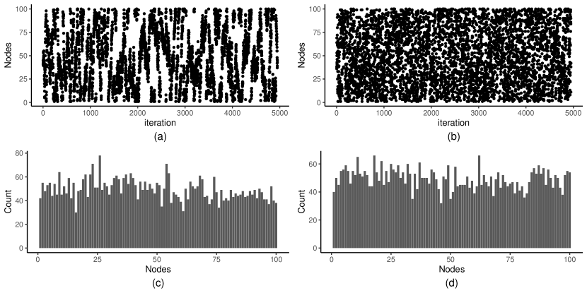
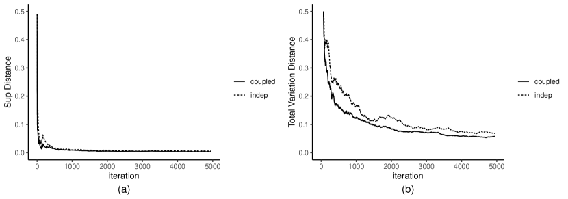
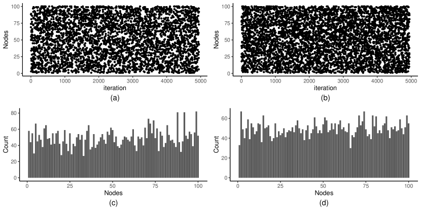
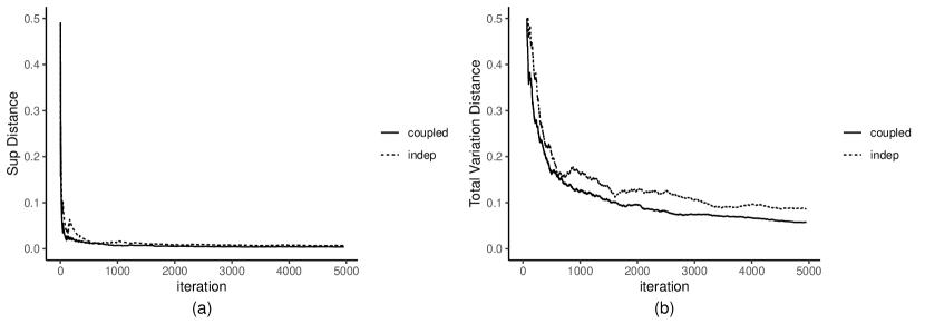
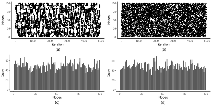
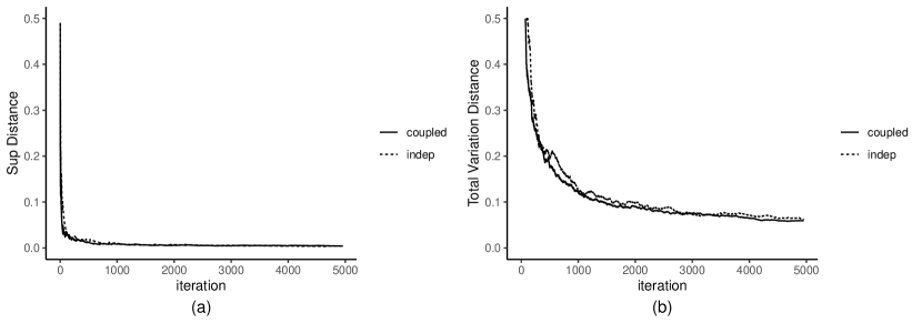
We numerically confirm that the parallel tempering accelerates the convergence of the distribution of the target chain to the uniform distribution. In this study, we compare the convergence speed of the target chain distribution with and without the parallel tempering. Four types of graphs with 100 nodes are used in simulation: i) circulant graph C1011superscriptsubscript𝐶1011C_{101}^{1} with one jump (Here, the number of nodes is 101 because the graph should not be bipartite.), ii) circulant graph C1001,2,3superscriptsubscript𝐶100123C_{100}^{1,2,3} with three jumps, iii) random 3-regular graph, and iv) the graph generated by the Watts-Strogatz small-world model. First, we generate two pairs of Markov chains on each graph. One is composed of two independent chains with transition probabilities PP{\rm P} and QQ{\rm Q}. The other consists of two chains with transition probabilities PP{\rm P} and QQ{\rm Q} that are Metropolis-coupled. To remove the effect of the initial value, we discard the first 5,000 samples. Then, we take only one sample per 100 samples to reduce the correlation between neighboring samples. Finally, we calculate the Lsubscript𝐿L_{\infty}-distance and the total variation distance between the distribution of the target chain and the uniform distribution. The two metrics are defined as follows : for distributions f,g:V[0,1]:𝑓𝑔𝑉01f,g:V\rightarrow[0,1] on the set V={1,2,,n}𝑉12𝑛V=\{1,2,\ldots,n\} of nodes, the Lsubscript𝐿L_{\infty}-distance is defined as dsup(f,g)=maxvV|f(v)g(v)|,subscript𝑑sup𝑓𝑔subscript𝑣𝑉𝑓𝑣𝑔𝑣d_{\rm sup}(f,g)=\max_{v\in V}\left|f(v)-g(v)\right|, and the total variation distance is defined as dtv(f,g)=maxAV|f(A)g(A)|=12vV|f(v)g(v)|.subscript𝑑tv𝑓𝑔subscript𝐴𝑉𝑓𝐴𝑔𝐴12subscript𝑣𝑉𝑓𝑣𝑔𝑣d_{\rm tv}(f,g)=\max_{A\subseteq V}\left|f(A)-g(A)\right|=\frac{1}{2}\sum_{v\in V}\left|f(v)-g(v)\right|. The results are reported in Appendix B.

4 Numerical study

In this section, we numerically investigate the sizes and powers of the proposed independence test procedure based on the RP statistics for bivariate right- and interval-censored data. To generate correlated bivariate survival times, we consider Clayton and Frank copula models as in Kim et al. (2015). To be specific, let F(x,y)𝐹𝑥𝑦F(x,y) be a joint cumulative distribution function of complete observation (X,Y)superscript𝑋superscript𝑌(X^{*},Y^{*}), and FX(x)subscript𝐹𝑋𝑥F_{X}(x) and FY(y)subscript𝐹𝑌𝑦F_{Y}(y) be marginal cumulative distribution functions of Xsuperscript𝑋X^{*} and Ysuperscript𝑌Y^{*}, respectively. The Clayton copula model (Clayton, 1978) is defined as

F(x,y)=((FX(x))α+(FY(y))α1)1/α,𝐹𝑥𝑦superscriptsuperscriptsubscript𝐹𝑋𝑥𝛼superscriptsubscript𝐹𝑌𝑦𝛼11𝛼F(x,y)=\big{(}(F_{X}(x))^{-\alpha}+(F_{Y}(y))^{-\alpha}-1\big{)}^{-1/\alpha},

where α=2τ/(1τ)>0𝛼2𝜏1𝜏0\alpha=2\tau/(1-\tau)>0 and τ𝜏\tau denotes the Kendall’s τ𝜏\tau. The Frank copula model (Frank, 1979) is defined as

F(x,y)=1βlog(1+(eβFX(x)1)(eβFY(y)1)eβ1),𝐹𝑥𝑦1𝛽1superscript𝑒𝛽subscript𝐹𝑋𝑥1superscript𝑒𝛽subscript𝐹𝑌𝑦1superscript𝑒𝛽1F(x,y)=-\frac{1}{\beta}\log\left(1+\frac{(e^{-\beta F_{X}(x)}-1)(e^{-\beta F_{Y}(y)}-1)}{e^{-\beta}-1}\right),

where β>0𝛽0\beta>0 controls dependency of Xsuperscript𝑋X^{*} and Ysuperscript𝑌Y^{*}. It is known that τ=1+4β1(D1(β)1)𝜏14superscript𝛽1subscript𝐷1𝛽1\tau=1+4\beta^{-1}(D_{1}(\beta)-1), where D1(β)=β10βt(et1)1𝑑tsubscript𝐷1𝛽superscript𝛽1superscriptsubscript0𝛽𝑡superscriptsuperscript𝑒𝑡11differential-d𝑡D_{1}(\beta)=\beta^{-1}\int_{0}^{\beta}t(e^{t}-1)^{-1}~{}dt is the first-order Debye function. With the given copula model, we first generate (U1,U2)subscript𝑈1subscript𝑈2(U_{1},U_{2}) from the given copula model and apply the inverse transformation of marginal distribution functions (FX1(U1),FY1(U2))superscriptsubscript𝐹𝑋1subscript𝑈1superscriptsubscript𝐹𝑌1subscript𝑈2(F_{X}^{-1}(U_{1}),F_{Y}^{-1}(U_{2})). For marginal distributions of Xsuperscript𝑋X^{*} and Ysuperscript𝑌Y^{*}, we consider FX(x)=1e0.1xsubscript𝐹𝑋𝑥1superscript𝑒0.1𝑥F_{X}(x)=1-e^{-0.1x} and FY(y)=1e0.1ysubscript𝐹𝑌𝑦1superscript𝑒0.1𝑦F_{Y}(y)=1-e^{-0.1y} following Kim et al. (2015). In this study, the bivariate survival times {(Xi,Yi)}i=1nsuperscriptsubscriptsuperscriptsubscript𝑋𝑖superscriptsubscript𝑌𝑖𝑖1𝑛\{(X_{i}^{*},Y_{i}^{*})\}_{i=1}^{n} are generated with τ=0,1/5,1/3𝜏01513\tau=0,~{}1/5,~{}1/3 and n=50,100𝑛50100n=50,~{}100, where τ=1/5,1/3𝜏1513\tau=1/5,~{}1/3 are corresponding to α=1/2,1𝛼121\alpha=1/2,~{}1 for Clayton copula and β1.8609,3.3058𝛽1.86093.3058\beta\approx 1.8609,~{}3.3058 for Frank copula, respectively. We evaluate the sizes and powers based on 500 simulations, where both the number of permutation for approximating null distribution and the number of MC samples from the restricted permutation space are set as 1000.

4.1 Bivariate right-censored data

To generate right-censored data, we assume that the censoring times Xicsuperscriptsubscript𝑋𝑖𝑐X_{i}^{c} and Yicsuperscriptsubscript𝑌𝑖𝑐Y_{i}^{c} are independent with the event times Xisuperscriptsubscript𝑋𝑖X_{i}^{*} and Yisuperscriptsubscript𝑌𝑖Y_{i}^{*} and follows the uniform distribution U(0,cR)𝑈0subscript𝑐𝑅U(0,c_{R}). With the generated complete bivariate observations {(Xi,Yi),i=1,2,,n}formulae-sequencesuperscriptsubscript𝑋𝑖superscriptsubscript𝑌𝑖𝑖12𝑛\{(X_{i}^{*},Y_{i}^{*}),i=1,2,\ldots,n\} and censoring times {(Xic,Yic),i=1,2,,n}formulae-sequencesuperscriptsubscript𝑋𝑖𝑐superscriptsubscript𝑌𝑖𝑐𝑖12𝑛\{(X_{i}^{c},Y_{i}^{c}),i=1,2,\ldots,n\}, we define the right-censored data {(Xi,δiX),(Yi,δiY),i=1,2,,n}formulae-sequencesubscript𝑋𝑖superscriptsubscript𝛿𝑖𝑋subscript𝑌𝑖superscriptsubscript𝛿𝑖𝑌𝑖12𝑛\{(X_{i},\delta_{i}^{X}),(Y_{i},\delta_{i}^{Y}),i=1,2,\ldots,n\} with Xi=min(Xi,Xic)subscript𝑋𝑖superscriptsubscript𝑋𝑖superscriptsubscript𝑋𝑖𝑐X_{i}=\min(X_{i}^{*},X_{i}^{c}), δiX=I(XiXic)superscriptsubscript𝛿𝑖𝑋𝐼superscriptsubscript𝑋𝑖superscriptsubscript𝑋𝑖𝑐\delta_{i}^{X}=I(X_{i}^{*}\leq X_{i}^{c}), Yi=min(Yi,Yic)subscript𝑌𝑖superscriptsubscript𝑌𝑖superscriptsubscript𝑌𝑖𝑐Y_{i}=\min(Y_{i}^{*},Y_{i}^{c}), and δiY=I(YiYic)superscriptsubscript𝛿𝑖𝑌𝐼superscriptsubscript𝑌𝑖superscriptsubscript𝑌𝑖𝑐\delta_{i}^{Y}=I(Y_{i}^{*}\leq Y_{i}^{c}). We consider cR=9,15subscript𝑐𝑅915c_{R}=9,~{}15, where censoring rates with cR=9,15subscript𝑐𝑅915c_{R}=9,~{}15 are 65.8% and 51.8%, respectively.

For testing the independence of the bivariate right-censored data, several methods are introduced in the literature. Among the existing methods, for the purpose of comparison, we consider two testing procedures using Kendall’s tau proposed by Oakes (1982) and Kim et al. (2015). We denote the Kendall’s tau defined in Oakes (1982) and Kim et al. (2015) as τ^Osuperscript^𝜏𝑂\hat{\tau}^{O} and τ^NPsuperscript^𝜏𝑁𝑃\hat{\tau}^{NP}, respectively. In Oakes (1982), the Kendall’s tau τ^Osuperscript^𝜏O\hat{\tau}^{\rm O} for the right-censored data is defined as

τ^O=i<jaijbijn(n1)/2,superscript^𝜏𝑂subscript𝑖𝑗subscript𝑎𝑖𝑗subscript𝑏𝑖𝑗𝑛𝑛12\hat{\tau}^{O}=\frac{\sum_{i<j}a_{ij}b_{ij}}{n(n-1)/2}, (7)

where aij=1subscript𝑎𝑖𝑗1a_{ij}=1 if Xi>Xjsubscript𝑋𝑖subscript𝑋𝑗X_{i}>X_{j} and (δiX,δjX){(0,1),(1,1)}superscriptsubscript𝛿𝑖𝑋superscriptsubscript𝛿𝑗𝑋0111(\delta_{i}^{X},\delta_{j}^{X})\in\{(0,1),(1,1)\}, 11-1 if Xi<Xjsubscript𝑋𝑖subscript𝑋𝑗X_{i}<X_{j} and (δiX,δjX){(1,0),(1,1)}superscriptsubscript𝛿𝑖𝑋superscriptsubscript𝛿𝑗𝑋1011(\delta_{i}^{X},\delta_{j}^{X})\in\{(1,0),(1,1)\}, and 00 otherwise, and bijsubscript𝑏𝑖𝑗b_{ij} is similarly defined with Yisubscript𝑌𝑖Y_{i} and Yjsubscript𝑌𝑗Y_{j}. In Kim et al. (2015), the Kendall’s tau τ^NPsuperscript^𝜏𝑁𝑃\hat{\tau}^{NP} is defined as

τ^NP=i,ja~ijb~ij(i,ja~ij2)(i,jb~ij2),superscript^𝜏𝑁𝑃subscript𝑖𝑗subscript~𝑎𝑖𝑗subscript~𝑏𝑖𝑗subscript𝑖𝑗superscriptsubscript~𝑎𝑖𝑗2subscript𝑖𝑗superscriptsubscript~𝑏𝑖𝑗2\hat{\tau}^{NP}=\frac{\sum_{i,j}\tilde{a}_{ij}\tilde{b}_{ij}}{\sqrt{(\sum_{i,j}\tilde{a}_{ij}^{2})(\sum_{i,j}\tilde{b}_{ij}^{2})}}, (8)

where a~ij=2P(Xi>Xj|(Xi,δiX),(Xj,δjX))1subscript~𝑎𝑖𝑗2𝑃superscriptsubscript𝑋𝑖conditionalsuperscriptsubscript𝑋𝑗subscript𝑋𝑖superscriptsubscript𝛿𝑖𝑋subscript𝑋𝑗superscriptsubscript𝛿𝑗𝑋1\tilde{a}_{ij}=2P\big{(}X_{i}^{*}>X_{j}^{*}~{}|~{}(X_{i},\delta_{i}^{X}),(X_{j},\delta_{j}^{X})\big{)}-1 and b~ij=2P(Yi>Yj|(Yi,δiY),(Yj,δjY))1subscript~𝑏𝑖𝑗2𝑃superscriptsubscript𝑌𝑖conditionalsuperscriptsubscript𝑌𝑗subscript𝑌𝑖superscriptsubscript𝛿𝑖𝑌subscript𝑌𝑗superscriptsubscript𝛿𝑗𝑌1\tilde{b}_{ij}=2P\big{(}Y_{i}^{*}>Y_{j}^{*}~{}|~{}(Y_{i},\delta_{i}^{Y}),(Y_{j},\delta_{j}^{Y})\big{)}-1. The conditional probabilities {a~ij}subscript~𝑎𝑖𝑗\{\tilde{a}_{ij}\} and {b~ij}subscript~𝑏𝑖𝑗\{\tilde{b}_{ij}\} are estimated by the nonparametric maximum likelihood estimators (NPMLEs) of the marginal distribution functions FX(x)subscript𝐹𝑋𝑥F_{X}(x) and FY(y)subscript𝐹𝑌𝑦F_{Y}(y). In this paper, we estimate the marginal distribution functions FX(x)subscript𝐹𝑋𝑥F_{X}(x) and FY(y)subscript𝐹𝑌𝑦F_{Y}(y) with the R function icfit in R package interval. The test statistics ZO=τ^O/Var(τ^O)subscript𝑍𝑂superscript^𝜏𝑂Varsuperscript^𝜏𝑂Z_{O}=\hat{\tau}^{O}/\sqrt{{\rm Var}(\hat{\tau}^{O})} and ZNP=τ^NP/Var(τ^NP)subscript𝑍𝑁𝑃superscript^𝜏𝑁𝑃Varsuperscript^𝜏𝑁𝑃Z_{NP}=\hat{\tau}^{NP}/\sqrt{{\rm Var}(\hat{\tau}^{NP})} are used for testing independence, where their asymptotic null distribution is the standard normal distribution.

To compare fairly, we evaluate p-values of τ^Osuperscript^𝜏𝑂\hat{\tau}^{O}, τ^NPsuperscript^𝜏𝑁𝑃\hat{\tau}^{NP} and τ^RPsuperscript^𝜏𝑅𝑃\hat{\tau}^{RP} with the approximated null distribution by permutation as well as their asymptotic null distributions. The RP statistic τ^RPsuperscript^𝜏𝑅𝑃\hat{\tau}^{RP} is the mean of {τ(RbX,RbY):b=1,,B}conditional-set𝜏superscriptsubscript𝑅𝑏𝑋superscriptsubscript𝑅𝑏𝑌𝑏1𝐵\{\tau(R_{b}^{X},R_{b}^{Y}):b=1,\ldots,B\} and then ZRP=τ^RP/Var(τ^RP)dN(0,1)subscript𝑍𝑅𝑃superscript^𝜏𝑅𝑃Varsuperscript^𝜏𝑅𝑃superscript𝑑𝑁01Z_{RP}=\hat{\tau}^{RP}/\sqrt{{\rm Var}(\hat{\tau}^{RP})}\stackrel{{\scriptstyle d}}{{\to}}N(0,1) by the central limit theorem. We estimate variances of τ^Osuperscript^𝜏𝑂\hat{\tau}^{O}, τ^NPsuperscript^𝜏𝑁𝑃\hat{\tau}^{NP}, and τ^RPsuperscript^𝜏𝑅𝑃\hat{\tau}^{RP} by the permutation and plug in the variance estimates in ZOsubscript𝑍𝑂Z_{O}, ZNPsubscript𝑍𝑁𝑃Z_{NP}, and ZRPsubscript𝑍𝑅𝑃Z_{RP}. We report the bias ((1/m)i=1mτ^iτ1𝑚superscriptsubscript𝑖1𝑚subscript^𝜏𝑖𝜏(1/m)\sum_{i=1}^{m}\hat{\tau}_{i}-\tau), the mean squared error (MSE, (1/m)i=1m(τ^iτ)21𝑚superscriptsubscript𝑖1𝑚superscriptsubscript^𝜏𝑖𝜏2(1/m)\sum_{i=1}^{m}(\hat{\tau}_{i}-\tau)^{2}), empirical powers evaluated by asymptotic null distribution (EP-A) and empirical powers evaluated by permutation (EP-P) in Table 1, where m𝑚m is the number of simulations, EP-A and EP-P are calculated by the ratios of the number of rejections to the number of simulations with p-values from the asymptotic null distribution and the approximated null distribution by permutation, respectively.

From Table 1, we observed several features. First, the asymptotic null distributions and approximated null distribution by permutation are similar and well-approximated to the true null distribution since the sizes of independence test of τ^Osuperscript^𝜏𝑂\hat{\tau}^{O}, τ^NPsuperscript^𝜏𝑁𝑃\hat{\tau}^{NP}, and τ^RPsuperscript^𝜏𝑅𝑃\hat{\tau}^{RP} are well-controlled with the given level 0.050.050.05, and all EP-A and EP-P values are similar. Second, powers of all three methods increase when the censoring rates decrease from 65.8% (cR=9subscript𝑐𝑅9c_{R}=9) to 51.8% (cR=15subscript𝑐𝑅15c_{R}=15) except the case of (n=50,τ=1/5)formulae-sequence𝑛50𝜏15(n=50,\tau=1/5). In the case (n=50,τ=1/5)formulae-sequence𝑛50𝜏15(n=50,\tau=1/5), the decrements of the powers of all three methods from cR=9subscript𝑐𝑅9c_{R}=9 to cR=15subscript𝑐𝑅15c_{R}=15 are small. For instance, the decrement of powers of τ^Osuperscript^𝜏𝑂\hat{\tau}^{O}, τ^NPsuperscript^𝜏𝑁𝑃\hat{\tau}^{NP}, and τ^RPsuperscript^𝜏𝑅𝑃\hat{\tau}^{RP} are 0.040.040.04, 0.0120.0120.012, 0.0320.0320.032 in EP-P, respectively. Third, the biases and MSEs of all three methods increases as the true τ𝜏\tau increases but those of τ^NPsuperscript^𝜏𝑁𝑃\hat{\tau}^{NP} are preserved at lower levels than those of τ^Osuperscript^𝜏𝑂\hat{\tau}^{O} and τ^RPsuperscript^𝜏𝑅𝑃\hat{\tau}^{RP}. For example, for the case of (n=50,τ=1/3,cR=15)formulae-sequence𝑛50formulae-sequence𝜏13subscript𝑐𝑅15(n=50,\tau=1/3,c_{R}=15), the biases of τ^Osuperscript^𝜏𝑂\hat{\tau}^{O}, τ^NPsuperscript^𝜏𝑁𝑃\hat{\tau}^{NP}, and τ^RPsuperscript^𝜏𝑅𝑃\hat{\tau}^{RP} are 0.13880.1388-0.1388, 0.03150.03150.0315, and 0.12010.1201-0.1201, respectively. The increment of bias of τ^Osuperscript^𝜏𝑂\hat{\tau}^{O} is caused by a fixed denominator n(n1)/2𝑛𝑛12n(n-1)/2 since the summation of the scores in the numerator is only on the comparable pairs, where the number of comparable pairs can be much smaller than n(n1)/2𝑛𝑛12n(n-1)/2. For τ^RPsuperscript^𝜏𝑅𝑃\hat{\tau}^{RP}, the increment of bias of τ^RPsuperscript^𝜏𝑅𝑃\hat{\tau}^{RP} is caused by the characteristic that τ^RPsuperscript^𝜏𝑅𝑃\hat{\tau}^{RP} under-estimates τ𝜏\tau when τ0𝜏0\tau\neq 0 as we mentioned in the previous section. The bias of τ^RPsuperscript^𝜏𝑅𝑃\hat{\tau}^{RP} is the smallest among three methods when τ=0𝜏0\tau=0. Finally, in view of powers of testing independence, no method outperforms others for all cases. Under Clayton copula, the powers of τ^Osuperscript^𝜏𝑂\hat{\tau}^{O} is greater than those of the other two methods, and the power of τ^RPsuperscript^𝜏𝑅𝑃\hat{\tau}^{RP} is greater than τ^NPsuperscript^𝜏𝑁𝑃\hat{\tau}^{NP}. Under Frank copula, the powers of τ^NPsuperscript^𝜏𝑁𝑃\hat{\tau}^{NP} is often similar to or larger than those of τ^Osuperscript^𝜏𝑂\hat{\tau}^{O} and τ^RPsuperscript^𝜏𝑅𝑃\hat{\tau}^{RP}. For this case, our numerical study recommends the use τ^Osuperscript^𝜏𝑂\hat{\tau}^{O}, which is the best under Clayton copula and the second-best under Frank copula. However, the powers of all three methods are not significantly different.

4.2 Bivariate interval-censored data

Bivariate case-2 interval-censored observations are generated by three steps as in generating bivariate right-censored observations. First, we generate complete bivariate observations {(Xi,Yi)}i=1nsuperscriptsubscriptsuperscriptsubscript𝑋𝑖superscriptsubscript𝑌𝑖𝑖1𝑛\{(X_{i}^{*},Y_{i}^{*})\}_{i=1}^{n} based on the given copula model and the inverse transformation of marginal distribution function. Second, under the non-informative censoring assumption, we independently generate observation times (Ti1X,Ti2X)superscriptsubscript𝑇𝑖1𝑋superscriptsubscript𝑇𝑖2𝑋(T_{i1}^{X},T_{i2}^{X}) and (Ti1Y,Ti2Y)superscriptsubscript𝑇𝑖1𝑌superscriptsubscript𝑇𝑖2𝑌(T_{i1}^{Y},T_{i2}^{Y}). Finally, the bivariate interval-censored observations are defined as {((Ti1X,Ti2X,δi1X,δi2X),(Ti1Y,Ti2Y,δi1Y,δi2Y))}superscriptsubscript𝑇𝑖1𝑋superscriptsubscript𝑇𝑖2𝑋superscriptsubscript𝛿𝑖1𝑋superscriptsubscript𝛿𝑖2𝑋superscriptsubscript𝑇𝑖1𝑌superscriptsubscript𝑇𝑖2𝑌superscriptsubscript𝛿𝑖1𝑌superscriptsubscript𝛿𝑖2𝑌\big{\{}\big{(}(T_{i1}^{X},T_{i2}^{X},\delta_{i1}^{X},\delta_{i2}^{X}),(T_{i1}^{Y},T_{i2}^{Y},\delta_{i1}^{Y},\delta_{i2}^{Y})\big{)}\big{\}}, where δi1X=I(XiTi1X)superscriptsubscript𝛿𝑖1𝑋𝐼superscriptsubscript𝑋𝑖superscriptsubscript𝑇𝑖1𝑋\delta_{i1}^{X}=I(X_{i}^{*}\leq T_{i1}^{X}), δi2X=I(Ti1X<XiTi2X)superscriptsubscript𝛿𝑖2𝑋𝐼superscriptsubscript𝑇𝑖1𝑋superscriptsubscript𝑋𝑖superscriptsubscript𝑇𝑖2𝑋\delta_{i2}^{X}=I(T_{i1}^{X}<X_{i}^{*}\leq T_{i2}^{X}), and δi1Ysuperscriptsubscript𝛿𝑖1𝑌\delta_{i1}^{Y} and δi2Ysuperscriptsubscript𝛿𝑖2𝑌\delta_{i2}^{Y} are similarly defined. For observation times (T1,T2)subscript𝑇1subscript𝑇2(T_{1},T_{2}), we consider two scenarios:

  • (C1): Observation times are from uniform distribution, which assumes that the observation times are not pre-scheduled. In this scenario, we generate Ti1subscript𝑇𝑖1T_{i1} and Qisubscript𝑄𝑖Q_{i} independently from U(0,cL)𝑈0subscript𝑐𝐿U(0,c_{L}) and U(0,cR)𝑈0subscript𝑐𝑅U(0,c_{R}), respectively. Then, we obtain Ti2=Ti1+Qisubscript𝑇𝑖2subscript𝑇𝑖1subscript𝑄𝑖T_{i2}=T_{i1}+Q_{i} for i=1,,n𝑖1𝑛i=1,\ldots,n. We consider cL=3subscript𝑐𝐿3c_{L}=3 and cR=6,12subscript𝑐𝑅612c_{R}=6,12, where the rates of left, right, and interval censoring are (13.5%, 65% 21.5%) and (13.5%, 50.5%, 36%) for cR=6,12subscript𝑐𝑅612c_{R}=6,12, respectively.

  • (C2): Observation times are pre-scheduled. In this scenario, we assume that observation is conducted every three month and a total observation period is cRsubscript𝑐𝑅c_{R}. We further assume an ideal case in the sense that all patients are observed at given observation times and stop when the event occurs. Thus, (Ti1,Ti2){(0,3],(3,6],,(cR,)}subscript𝑇𝑖1subscript𝑇𝑖20336subscript𝑐𝑅(T_{i1},T_{i2})\in\big{\{}(0,3],(3,6],\ldots,(c_{R},\infty)\}. We consider cR=9,15subscript𝑐𝑅915c_{R}=9,15, where the rates of right, and interval censoring are (41%, 59%) and (22.5%, 77.5%) for cR=9,15subscript𝑐𝑅915c_{R}=9,15, respectively.

For the independence test of the bivariate interval-censored data, we consider two existing procedures using Kendall’s tau proposed by Betensky and Finkelstein (1999a) and Kim et al. (2015). Note that we exclude the two-stage estimation procedure proposed by Sun et al. (2006) in the comparison of testing independence of the bivariate interval-censored data following the comment in Kim et al. (2015) that the two-stage estimation is not valid for testing independence. As in the right-censored data, we denote the estimator and the method of Kim et al. (2015) as τ^NPsuperscript^𝜏𝑁𝑃\hat{\tau}^{NP}. Here, we omit the details of τ^NPsuperscript^𝜏𝑁𝑃\hat{\tau}^{NP} since basic idea and notations are the same as the ones in the bivariate right-censored data. We refer to Section 3.2 in Kim et al. (2015) for the estimation of conditional probability in a~ijsubscript~𝑎𝑖𝑗\tilde{a}_{ij} and b~ijsubscript~𝑏𝑖𝑗\tilde{b}_{ij}. Betensky and Finkelstein (1999a) extend Kendall’s tau to the bivariate interval-censored data based on the NPMLE of the joint survival function S(x,y)𝑆𝑥𝑦S(x,y) and the multiple imputations. We use a notation τ^MIsuperscript^𝜏𝑀𝐼\hat{\tau}^{MI} to denote the estimator and the method by Betensky and Finkelstein (1999a). To be specific, let {((LiX,RiX],(LiY,RiY)),i=1,2,,n}formulae-sequencesuperscriptsubscript𝐿𝑖𝑋superscriptsubscript𝑅𝑖𝑋superscriptsubscript𝐿𝑖𝑌superscriptsubscript𝑅𝑖𝑌𝑖12𝑛\big{\{}\big{(}(L_{i}^{X},R_{i}^{X}],(L_{i}^{Y},R_{i}^{Y})\big{)},i=1,2,\ldots,n\big{\}} be interval-censored observations. In the procedure τ^MIsuperscript^𝜏𝑀𝐼\hat{\tau}^{MI}, the Kendall’s tau τ^MIsuperscript^𝜏𝑀𝐼\hat{\tau}^{MI} is estimated by the following three steps. In the first step, the joint survival function S(x,y)𝑆𝑥𝑦S(x,y) is estimated by the NPMLE. Second step generates M𝑀M datasets where the interval-censored observations of {((LiX,RiX],(LiY,RiY)),i=1,2,,n}formulae-sequencesuperscriptsubscript𝐿𝑖𝑋superscriptsubscript𝑅𝑖𝑋superscriptsubscript𝐿𝑖𝑌superscriptsubscript𝑅𝑖𝑌𝑖12𝑛\big{\{}\big{(}(L_{i}^{X},R_{i}^{X}],(L_{i}^{Y},R_{i}^{Y})\big{)},i=1,2,\ldots,n\big{\}} are imputed by ((Li,(k)X,Ri,(k)X],(Li,(k)Y,Ri,(k)Y])superscriptsubscript𝐿𝑖𝑘𝑋superscriptsubscript𝑅𝑖𝑘𝑋superscriptsubscript𝐿𝑖𝑘𝑌superscriptsubscript𝑅𝑖𝑘𝑌\big{(}(L_{i,(k)}^{X},R_{i,(k)}^{X}],(L_{i,(k)}^{Y},R_{i,(k)}^{Y}]\big{)} for k=1,,M𝑘1𝑀k=1,\ldots,M uniformly generated from the conditional survival distribution of ((Li,(k)X,Ri,(k)X],(Li,(k)Y,Ri,(k)Y])superscriptsubscript𝐿𝑖𝑘𝑋superscriptsubscript𝑅𝑖𝑘𝑋superscriptsubscript𝐿𝑖𝑘𝑌superscriptsubscript𝑅𝑖𝑘𝑌\big{(}(L_{i,(k)}^{X},R_{i,(k)}^{X}],(L_{i,(k)}^{Y},R_{i,(k)}^{Y}]\big{)} given (Li,(k)X,Ri,(k)X]×(Li,(k)Y,Ri,(k)Y](LiX,RiX]×(LiY,RiY)superscriptsubscript𝐿𝑖𝑘𝑋superscriptsubscript𝑅𝑖𝑘𝑋superscriptsubscript𝐿𝑖𝑘𝑌superscriptsubscript𝑅𝑖𝑘𝑌superscriptsubscript𝐿𝑖𝑋superscriptsubscript𝑅𝑖𝑋superscriptsubscript𝐿𝑖𝑌superscriptsubscript𝑅𝑖𝑌(L_{i,(k)}^{X},R_{i,(k)}^{X}]\times(L_{i,(k)}^{Y},R_{i,(k)}^{Y}]\subset(L_{i}^{X},R_{i}^{X}]\times(L_{i}^{Y},R_{i}^{Y}). In the third step, the estimator τ^MIsuperscript^𝜏𝑀𝐼\hat{\tau}^{MI} is obtained by

τ^MI=1Mk=1Mi<jϕij(k)n(n1)/2,superscript^𝜏𝑀𝐼1𝑀superscriptsubscript𝑘1𝑀subscript𝑖𝑗superscriptsubscriptitalic-ϕ𝑖𝑗𝑘𝑛𝑛12\hat{\tau}^{MI}=\frac{1}{M}\sum_{k=1}^{M}\frac{\sum\sum_{i<j}\phi_{ij}^{(k)}}{n(n-1)/2},

where

ϕij(k)={1if Ri,(k)X<Lj,(k)X,Ri,(k)Y<Lj,(k)Y or Rj,(k)X<Li,(k)X,Rj,(k)Y<Li,(k)Y,1if Ri,(k)X<Lj,(k)X,Li,(k)Y>Rj,(k)Y or Rj,(k)X<Li,(k)X,Lj,(k)Y>Ri,(k)Y,0otherwise.superscriptsubscriptitalic-ϕ𝑖𝑗𝑘cases1formulae-sequenceformulae-sequenceif superscriptsubscript𝑅𝑖𝑘𝑋superscriptsubscript𝐿𝑗𝑘𝑋superscriptsubscript𝑅𝑖𝑘𝑌superscriptsubscript𝐿𝑗𝑘𝑌 or superscriptsubscript𝑅𝑗𝑘𝑋superscriptsubscript𝐿𝑖𝑘𝑋superscriptsubscript𝑅𝑗𝑘𝑌superscriptsubscript𝐿𝑖𝑘𝑌1formulae-sequenceformulae-sequenceif superscriptsubscript𝑅𝑖𝑘𝑋superscriptsubscript𝐿𝑗𝑘𝑋superscriptsubscript𝐿𝑖𝑘𝑌superscriptsubscript𝑅𝑗𝑘𝑌 or superscriptsubscript𝑅𝑗𝑘𝑋superscriptsubscript𝐿𝑖𝑘𝑋superscriptsubscript𝐿𝑗𝑘𝑌superscriptsubscript𝑅𝑖𝑘𝑌0otherwise\phi_{ij}^{(k)}=\left\{\begin{array}[]{l l}1&\mbox{if }R_{i,(k)}^{X}<L_{j,(k)}^{X},R_{i,(k)}^{Y}<L_{j,(k)}^{Y}\mbox{ or }R_{j,(k)}^{X}<L_{i,(k)}^{X},R_{j,(k)}^{Y}<L_{i,(k)}^{Y},\\ -1&\mbox{if }R_{i,(k)}^{X}<L_{j,(k)}^{X},L_{i,(k)}^{Y}>R_{j,(k)}^{Y}\mbox{ or }R_{j,(k)}^{X}<L_{i,(k)}^{X},L_{j,(k)}^{Y}>R_{i,(k)}^{Y},\\ 0&\mbox{otherwise}.\end{array}\right.

In this paper, we set M=100𝑀100M=100 following Betensky and Finkelstein (1999a). With three measures τ^MIsuperscript^𝜏𝑀𝐼\hat{\tau}^{MI}, τ^NPsuperscript^𝜏𝑁𝑃\hat{\tau}^{NP}, and τ^RPsuperscript^𝜏𝑅𝑃\hat{\tau}^{RP}, we define test statistics ZMI=τ^MI/Var(τ^MI)subscript𝑍𝑀𝐼superscript^𝜏𝑀𝐼Varsuperscript^𝜏𝑀𝐼Z_{MI}=\hat{\tau}^{MI}/\sqrt{{\rm Var}(\hat{\tau}^{MI})}, ZNP=τ^NP/Var(τ^NP)subscript𝑍𝑁𝑃superscript^𝜏𝑁𝑃Varsuperscript^𝜏𝑁𝑃Z_{NP}=\hat{\tau}^{NP}/\sqrt{{\rm Var}(\hat{\tau}^{NP})}, ZRP=τ^RP/Var(τ^RP)subscript𝑍𝑅𝑃superscript^𝜏𝑅𝑃Varsuperscript^𝜏𝑅𝑃Z_{RP}=\hat{\tau}^{RP}/\sqrt{{\rm Var}(\hat{\tau}^{RP})}. Under the null hypothesis, the test statistics ZMIsubscript𝑍𝑀𝐼Z_{MI}, ZNPsubscript𝑍𝑁𝑃Z_{NP}, and ZRPsubscript𝑍𝑅𝑃Z_{RP} follow the standard normal distribution.

As in the bivariate right-censored data, we evaluate p-values of τ^MIsuperscript^𝜏𝑀𝐼\hat{\tau}^{MI}, τ^NPsuperscript^𝜏𝑁𝑃\hat{\tau}^{NP} and τ^RPsuperscript^𝜏𝑅𝑃\hat{\tau}^{RP} with their asymptotic null distributions and the approximated null distribution by permutation. We summarize the bias, MSE, EP-A, and EP-P in Tables 2 and 3 for the scenarios C1 and C2, respectively.

From Tables 2 and 3, we can easily see that τ^NPsuperscript^𝜏𝑁𝑃\hat{\tau}^{NP} and τ^RPsuperscript^𝜏𝑅𝑃\hat{\tau}^{RP} outperform τ^MIsuperscript^𝜏𝑀𝐼\hat{\tau}^{MI} in terms of the power of test and sizes of all three testing procedures are well-controlled. Thus, we focus on the comparison between τ^NPsuperscript^𝜏𝑁𝑃\hat{\tau}^{NP} and τ^RPsuperscript^𝜏𝑅𝑃\hat{\tau}^{RP}. First, for both scenarios 𝐂𝟏𝐂𝟏\bf C1 and 𝐂𝟐𝐂𝟐\bf C2, τ^RPsuperscript^𝜏𝑅𝑃\hat{\tau}^{RP} has smaller bias than τ^NPsuperscript^𝜏𝑁𝑃\hat{\tau}^{NP} when the true parameter τ=0𝜏0\tau=0 but has larger bias when τ0𝜏0\tau\neq 0. Our numerical study supports that the estimator τ^NPsuperscript^𝜏𝑁𝑃\hat{\tau}^{NP} is an unbiased estimator of Kendall’s tau for bivariate interval-censored data. For the ideal scenario 𝐂𝟐𝐂𝟐{\bf C2}, two testing procedures τ^RPsuperscript^𝜏𝑅𝑃\hat{\tau}^{RP} and τ^NPsuperscript^𝜏𝑁𝑃\hat{\tau}^{NP} have quite similar powers. In this scenario, the size of intervals is fixed and non-overlapped since all patients attend the pre-scheduled examination, and then the events are observed. Thus, τ^RPsuperscript^𝜏𝑅𝑃\hat{\tau}^{RP} and τ^NPsuperscript^𝜏𝑁𝑃\hat{\tau}^{NP} can fully utilize the observed intervals. This characteristic is supported by the positive increments of powers and the decrement of biases of τ^RPsuperscript^𝜏𝑅𝑃\hat{\tau}^{RP} and τ^NPsuperscript^𝜏𝑁𝑃\hat{\tau}^{NP} in terms of their absolute value from 𝐂𝟏𝐂𝟏\bf C1 to 𝐂𝟐𝐂𝟐\bf C2. Next, for the scenario 𝐂𝟏𝐂𝟏\bf C1, under Clayton copular, τ^RPsuperscript^𝜏𝑅𝑃\hat{\tau}^{RP} outperforms τ^NPsuperscript^𝜏𝑁𝑃\hat{\tau}^{NP}. On the other hand, under Frank copular, the powers of τ^NPsuperscript^𝜏𝑁𝑃\hat{\tau}^{NP} are similar to or slightly higher than those of τ^RPsuperscript^𝜏𝑅𝑃\hat{\tau}^{RP}. Thus, again as in the right-censored data, no method between τ^RPsuperscript^𝜏𝑅𝑃\hat{\tau}^{RP} and τ^NPsuperscript^𝜏𝑁𝑃\hat{\tau}^{NP} wins the other for all cases considered. However, we propose to use the RP statistic in the sense that the gain of the powers from τ^NPsuperscript^𝜏𝑁𝑃\hat{\tau}^{NP} to τ^RPsuperscript^𝜏𝑅𝑃\hat{\tau}^{RP} under Clayton copula is significant, while the power loss by using τ^RPsuperscript^𝜏𝑅𝑃\hat{\tau}^{RP} instead of τ^NPsuperscript^𝜏𝑁𝑃\hat{\tau}^{NP} is minor only under Frank copula.

5 Data examples

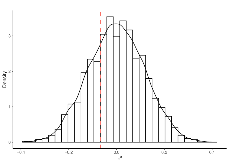
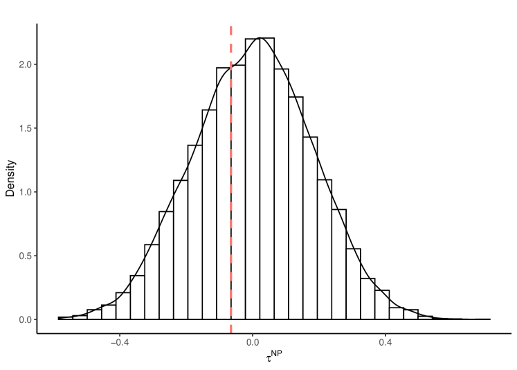
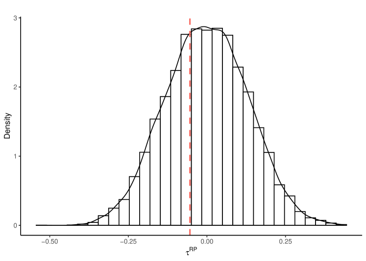
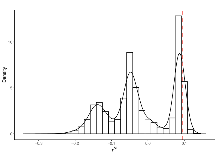
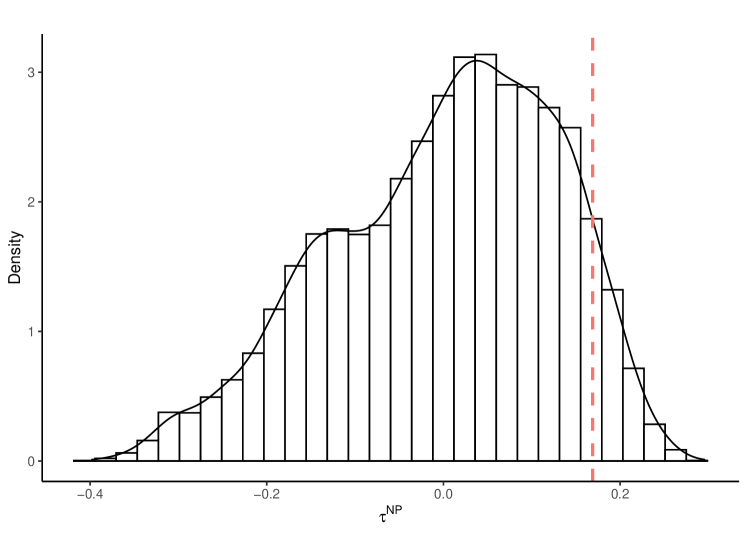
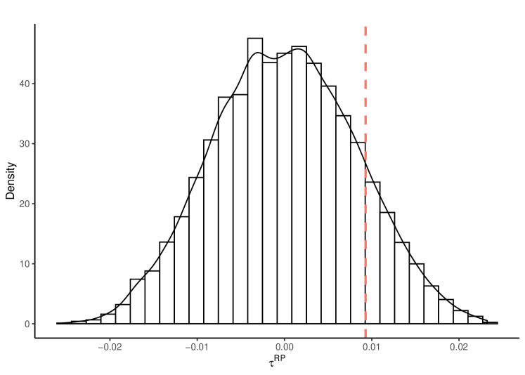
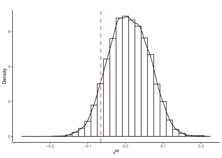
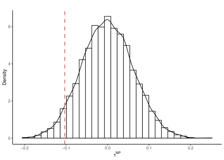
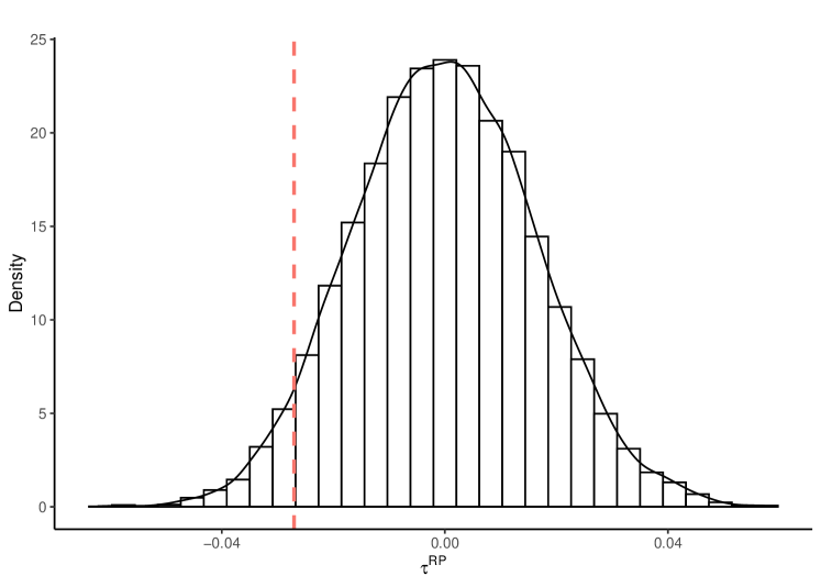
In this section, to provide real-data applications, we test the independence of the bivariate censored data with three real-data examples: a bivariate right-censored dataset, bivariate case-1, and case-2 interval-censored datasets. In addition, to check reliability of the proposed procedure, we consider τ^Osuperscript^𝜏𝑂\hat{\tau}^{O}, τ^NPsuperscript^𝜏𝑁𝑃\hat{\tau}^{NP}, and τ^RPsuperscript^𝜏𝑅𝑃\hat{\tau}^{RP} for the bivariate right-censored data and τ^MIsuperscript^𝜏𝑀𝐼\hat{\tau}^{MI}, τ^NPsuperscript^𝜏𝑁𝑃\hat{\tau}^{NP}, and τ^RPsuperscript^𝜏𝑅𝑃\hat{\tau}^{RP} for the bivariate interval-censored data as considered in the numerical study. The variances of the null distributions of the test statistics and the p-values evaluated by permutation are estimated by 10,000 permutations, and the RP statistic τ^RPsuperscript^𝜏𝑅𝑃\hat{\tau}^{RP} is obtained with 5,000 MCMC samples. All the results of testing independence are summarized in Table 4, and the null distributions approximated by permutation are plotted in Figure 1. Figure 1 shows that the null distribution of the RP statistic is well-approximated by the permutation procedure.

5.1 Leukemia remission data (right-censored data)

For the bivariate right-censored data, we consider the leukemia remission data set, which is a well-known bivariate right-censored data analyzed in Oakes (1982). The leukemia remission dataset consists of 21 paired lengths of remission maintenance with 6-MP (6-Mercaptopurine) and placebo from Phase II analysis in Freireich et al. (1963). For the purpose of the fair comparison and taking into account the existence of ties, we use the length of remission maintenance directly rather than their ranks in Oakes (1982), where the ties are broken by randomization and an assumption that the death at a given time always proceeds censoring at the same time.

In the leukemia remission data, the estimate τ^Osuperscript^𝜏𝑂\hat{\tau}^{O} of Kendall’s tau by Oakes (1982) is 0.06670.0667-0.0667, and its estimated variance by permutation is 0.01360.01360.0136. The p-values evaluated by the asymptotic null distribution (p-Asym) and permutation (p-Perm) of τ^Osuperscript^𝜏𝑂\hat{\tau}^{O} are 0.56800.56800.5680 and 0.57480.57480.5748, respectively. For τ^NPsuperscript^𝜏𝑁𝑃\hat{\tau}^{NP}, the estimate of Kendall’s tau by Kim et al. (2015) is 0.06520.0652-0.0652, and its variance is estimated as 0.03220.03220.0322. The p-Asym and p-Perm of τ^NPsuperscript^𝜏𝑁𝑃\hat{\tau}^{NP} are 0.71630.71630.7163 and 0.72000.72000.7200, respectively. For τ^RPsuperscript^𝜏𝑅𝑃\hat{\tau}^{RP}, the estimate of the proposed RP statistic is 0.05400.0540-0.0540, and its variance estimate is 0.01700.01700.0170. The p-Asym and p-Perm of τ^RPsuperscript^𝜏𝑅𝑃\hat{\tau}^{RP} are 0.67870.67870.6787 and 0.69980.69980.6998, respectively. The estimate of RP statistic is relatively smaller than the others τ^Osuperscript^𝜏𝑂\hat{\tau}^{O} and τ^NPsuperscript^𝜏𝑁𝑃\hat{\tau}^{NP} in terms of the absolute value. All three testing procedures consistently indicate that there is no evidence against H0subscript𝐻0H_{0}, which is the same conclusion of testing independence with the ranks of length of remission in Oakes (1982).

5.2 Animal tumorigenicity data (case-1 interval-censored data)

For the case-1 interval-censored data, we consider the animal tumorigenicity experiment dataset from National Toxicology Program (NTP) analyzed in Dunson and Dinse (2002). The experiment is designed to identify the effects of a chloroprene for carcinogenicity with 200 mice, which are separated into four groups, each of which consists of 50 mice and is exposed to the chloroprene of concentration 0, 12.8, 32, or 80 ppm for up to 2 years. In the experiment, all mice are either died by the natural cause or sacrificed at the end of 2 years. After death, the occurrence of tumors in various sites was determined through a pathologic examination.

In Dunson and Dinse (2002), the dataset provides the age at death and the number of mice at given age at death having no tumors, adrenal site only, lung site only, both sites. In this example, for the purpose of illustration of the inter-dependency, we test the independence of the occurrence times of tumors at the adrenal and the lung sites with the control group (chloroprene of concentration 0).

In the animal tumorigenicity data, the estimate τ^MIsuperscript^𝜏𝑀𝐼\hat{\tau}^{MI} of Kendall’s tau by Betensky and Finkelstein (1999a) is 0.09550.09550.0955, and its estimated variance by permutation is 0.00800.00800.0080. The p-Asym and p-Perm of τ^MIsuperscript^𝜏𝑀𝐼\hat{\tau}^{MI} are 0.28510.28510.2851 and 0.20460.20460.2046, respectively. For τ^NPsuperscript^𝜏𝑁𝑃\hat{\tau}^{NP}, the estimate of the Kendall’s tau by Kim et al. (2015) is 0.16890.16890.1689 and its variance estimate is 0.01630.01630.0163. The p-Asym and p-Perm of τ^NPsuperscript^𝜏𝑁𝑃\hat{\tau}^{NP} are 0.18530.18530.1853 and 0.19150.19150.1915, respectively. For τ^RPsuperscript^𝜏𝑅𝑃\hat{\tau}^{RP}, the estimate of the proposed RP statistic is 0.00930.00930.0093, and its variance estimate is 0.00010.00010.0001. The p-Asym and p-Perm of τ^RPsuperscript^𝜏𝑅𝑃\hat{\tau}^{RP} are 0.25190.25190.2519 and 0.26410.26410.2641, respectively. As observed in the numerical study, the p-Asym of τ^MIsuperscript^𝜏𝑀𝐼\hat{\tau}^{MI} is greater than the p-Perm of τ^MIsuperscript^𝜏𝑀𝐼\hat{\tau}^{MI} while the p-Asym and the p-Perm of the other two methods are similar. From the results of three testing independence procedures, there is no evidence that the occurrence times of cancer at the adrenal and the lung sites are correlated. Remark that the results of τ^MIsuperscript^𝜏𝑀𝐼\hat{\tau}^{MI} based on the null distribution approximated by permutation is consistent with others, but the permutation procedure poorly estimates the null distribution of τ^MIsuperscript^𝜏𝑀𝐼\hat{\tau}^{MI} as shown in Figure 1.

5.3 ACTG 181 data (case-2 interval-censored data)

For the case-2 interval-censored data, we consider the AIDS Clinical Trials Group protocol (ACTG 181) data analyzed by Betensky and Finkelstein (1999a). This study aims at identifying an association between the first time of shedding of cytomegalovirus (CMV) and colonization of mycobacterium avium complex (MAC). Since the investigation is conducted in the laboratory and many patients missed several pre-scheduled clinical visits, the observations of the first time of the event are interval-censored. In Betensky and Finkelstein (1999a), the association is estimated with 204 subjects which are tested for CMV shedding and MAC colonization at least once during the trial and did not have a prior CMV or MAC diagnosis. As in the analysis by Betensky and Finkelstein (1999a), we estimate τ^MIsuperscript^𝜏𝑀𝐼\hat{\tau}^{MI} with 100 imputed datasets.

In the ACTG 181 data, the estimate τ^MIsuperscript^𝜏𝑀𝐼\hat{\tau}^{MI} is 0.06540.0654-0.0654 and its estimated variance by permutation is 0.00290.00290.0029. The p-Asym and p-Perm of τ^MIsuperscript^𝜏𝑀𝐼\hat{\tau}^{MI} are 0.22600.22600.2260 and 0.17060.17060.1706, respectively. For τ^NPsuperscript^𝜏𝑁𝑃\hat{\tau}^{NP}, the estimate of Kendall’s tau is 0.10350.1035-0.1035, and its variance estimate is 0.00380.00380.0038. The p-Asym and p-Perm of τ^NPsuperscript^𝜏𝑁𝑃\hat{\tau}^{NP} are 0.09570.09570.0957 and 0.09600.09600.0960, respectively. For τ^RPsuperscript^𝜏𝑅𝑃\hat{\tau}^{RP}, the estimate of the proposed RP statistic is 0.02700.0270-0.0270, and its variance estimate is 0.00030.00030.0003. The p-Asym and p-Perm of τ^RPsuperscript^𝜏𝑅𝑃\hat{\tau}^{RP} are 0.09620.09620.0962 and 0.09540.09540.0954, respectively. Although the difference between the estimates τ^NPsuperscript^𝜏𝑁𝑃\hat{\tau}^{NP} and τ^RPsuperscript^𝜏𝑅𝑃\hat{\tau}^{RP} is relatively large (0.0765), the p-Asyms and p-Perms of τ^RPsuperscript^𝜏𝑅𝑃\hat{\tau}^{RP} and τ^NPsuperscript^𝜏𝑁𝑃\hat{\tau}^{NP} have similar values around 0.0960, which indicates that τ^RPsuperscript^𝜏𝑅𝑃\hat{\tau}^{RP} and τ^NPsuperscript^𝜏𝑁𝑃\hat{\tau}^{NP} lead the same conclusion that there is a significant correlation between the times of CMV shedding and MAC colonization when we consider the significance level α𝛼\alpha as 0.10. As stated in Betensky and Finkelstein (1999a), the results of three testing procedures indicate either a weak negative association between the times of CMV shedding and MAC colonization or the lack of sufficient power to detect the association.

6 Conclusion

In this paper, we propose a rank-based procedure to test the independence for bivariate incomplete data, which can be applicable to any type of incomplete data. The incomplete data defines a restricted permutation space of all possible ranks of the observations. We propose the average of Kendall’s tau over the ranks in the restricted permutation space as our test statistic. To evaluate the statistic and its reference distribution, we develop the MCMC procedure that obtains uniform samples on the restricted permutation space, which is applied to approximating the null distribution of the averaged Kendall’s tau.

Our proposal, the RP statistic, in this paper is generic and flexible enough in two ways. First, it is applicable to any type of incomplete data. Here, we focus on testing the independence of various types of bivariate censored data, which has been studied by different groups of researchers in the literature. Again, for the censored data, no assumptions are made for the underlying distribution and censoring mechanism. The RP statistic performs as good as other state-of-the-art methods for censoring mechanisms considered. Second, in this paper, we use the average of the uniform samples from the restricted rank space for comparison with the score-based procedure. However, there are many ways to make the summary of the uniform samples. Some examples would be the quantiles, median, or L-statistics, and they may perform better than the proposed RP statistic. This is left for future work.

Table 1: Biases, mean squared error (MSE), empirical power evaluated by asymptotic null distribution (EP-A), and empirical power evaluated by permutation (EP-P) for bivariate right-censored data.
cRsubscript𝑐𝑅c_{R} n𝑛n τ𝜏\tau Est. Clayton Frank
Bias MSE EP-A EP-P Bias MSE EP-A EP-B
999 505050 00 τ^Osuperscript^𝜏𝑂\hat{\tau}^{O} 0.0037 0.0016 0.036 0.034 0.0038 0.0016 0.036 0.034
τ^NPsuperscript^𝜏𝑁𝑃\hat{\tau}^{NP} 0.0093 0.0142 0.042 0.040 0.0096 0.0142 0.042 0.040
τ~RPsuperscript~𝜏𝑅𝑃\tilde{\tau}^{RP} 0.0042 0.0024 0.044 0.048 0.0045 0.0024 0.044 0.048
1/5151/5 τ^Osuperscript^𝜏𝑂\hat{\tau}^{O} -0.1078 0.0145 0.612 0.616 -0.1471 0.0239 0.276 0.286
τ^NPsuperscript^𝜏𝑁𝑃\hat{\tau}^{NP} 0.0299 0.0192 0.504 0.506 -0.0385 0.0188 0.266 0.262
τ~RPsuperscript~𝜏𝑅𝑃\tilde{\tau}^{RP} -0.0978 0.0132 0.556 0.552 -0.1389 0.0223 0.276 0.276
1/3131/3 τ^Osuperscript^𝜏𝑂\hat{\tau}^{O} -0.1859 0.0380 0.890 0.896 -0.2407 0.0604 0.606 0.608
τ^NPsuperscript^𝜏𝑁𝑃\hat{\tau}^{NP} 0.0393 0.0173 0.842 0.842 -0.0568 0.0189 0.644 0.648
τ~RPsuperscript~𝜏𝑅𝑃\tilde{\tau}^{RP} -0.1687 0.0324 0.874 0.876 -0.2263 0.0544 0.590 0.588
100100100 00 τ^Osuperscript^𝜏𝑂\hat{\tau}^{O} -0.0018 0.0008 0.044 0.046 -0.0018 0.0008 0.044 0.046
τ^NPsuperscript^𝜏𝑁𝑃\hat{\tau}^{NP} -0.0043 0.0069 0.040 0.042 -0.0046 0.0069 0.040 0.042
τ~RPsuperscript~𝜏𝑅𝑃\tilde{\tau}^{RP} -0.0017 0.0011 0.036 0.038 -0.0018 0.0011 0.036 0.038
1/5151/5 τ^Osuperscript^𝜏𝑂\hat{\tau}^{O} -0.1146 0.0145 0.798 0.804 -0.1415 0.0210 0.518 0.520
τ^NPsuperscript^𝜏𝑁𝑃\hat{\tau}^{NP} 0.0205 0.0091 0.716 0.714 -0.0244 0.0077 0.546 0.544
τ~RPsuperscript~𝜏𝑅𝑃\tilde{\tau}^{RP} -0.1044 0.0126 0.762 0.766 -0.1321 0.0189 0.480 0.478
1/3131/3 τ^Osuperscript^𝜏𝑂\hat{\tau}^{O} -0.1916 0.0385 0.988 0.984 -0.2356 0.0566 0.934 0.934
τ^NPsuperscript^𝜏𝑁𝑃\hat{\tau}^{NP} 0.0344 0.0095 0.972 0.972 -0.0449 0.0086 0.936 0.932
τ~RPsuperscript~𝜏𝑅𝑃\tilde{\tau}^{RP} -0.1742 0.0324 0.984 0.984 -0.2201 0.0499 0.908 0.908
151515 505050 00 τ^Osuperscript^𝜏𝑂\hat{\tau}^{O} 0.0036 0.0029 0.036 0.040 0.0036 0.0029 0.036 0.040
τ^NPsuperscript^𝜏𝑁𝑃\hat{\tau}^{NP} 0.0057 0.0132 0.038 0.034 0.0056 0.0132 0.038 0.034
τ~RPsuperscript~𝜏𝑅𝑃\tilde{\tau}^{RP} 0.0037 0.0041 0.038 0.046 0.0037 0.0041 0.038 0.046
1/5151/5 τ^Osuperscript^𝜏𝑂\hat{\tau}^{O} -0.0798 0.0105 0.582 0.576 -0.1160 0.0169 0.356 0.368
τ^NPsuperscript^𝜏𝑁𝑃\hat{\tau}^{NP} 0.0221 0.0149 0.498 0.494 -0.0184 0.0141 0.348 0.348
τ~RPsuperscript~𝜏𝑅𝑃\tilde{\tau}^{RP} -0.0694 0.0098 0.526 0.520 -0.1040 0.0155 0.358 0.348
1/3131/3 τ^Osuperscript^𝜏𝑂\hat{\tau}^{O} -0.1388 0.0239 0.934 0.936 -0.1889 0.0392 0.734 0.750
τ^NPsuperscript^𝜏𝑁𝑃\hat{\tau}^{NP} 0.0315 0.0135 0.886 0.884 -0.0270 0.0131 0.754 0.758
τ~RPsuperscript~𝜏𝑅𝑃\tilde{\tau}^{RP} -0.1201 0.0197 0.916 0.914 -0.1679 0.0327 0.728 0.734
100100100 00 τ^Osuperscript^𝜏𝑂\hat{\tau}^{O} -0.0018 0.0015 0.048 0.048 -0.0020 0.0015 0.048 0.048
τ^NPsuperscript^𝜏𝑁𝑃\hat{\tau}^{NP} -0.0032 0.0066 0.050 0.052 -0.0035 0.0067 0.050 0.052
τ~RPsuperscript~𝜏𝑅𝑃\tilde{\tau}^{RP} -0.0014 0.0020 0.050 0.052 -0.0016 0.0021 0.052 0.054
1/5151/5 τ^Osuperscript^𝜏𝑂\hat{\tau}^{O} -0.0873 0.0097 0.810 0.818 -0.1084 0.0133 0.658 0.662
τ^NPsuperscript^𝜏𝑁𝑃\hat{\tau}^{NP} 0.0140 0.0079 0.728 0.722 -0.0044 0.0061 0.700 0.690
τ~RPsuperscript~𝜏𝑅𝑃\tilde{\tau}^{RP} -0.0754 0.0084 0.768 0.766 -0.0957 0.0113 0.634 0.638
1/3131/3 τ^Osuperscript^𝜏𝑂\hat{\tau}^{O} -0.1461 0.0237 0.994 0.994 -0.1839 0.0354 0.982 0.982
τ^NPsuperscript^𝜏𝑁𝑃\hat{\tau}^{NP} 0.0243 0.0074 0.992 0.992 -0.0167 0.0055 0.984 0.984
τ~RPsuperscript~𝜏𝑅𝑃\tilde{\tau}^{RP} -0.1262 0.0187 0.990 0.990 -0.1628 0.0286 0.966 0.972
Table 2: Biases, mean squared error (MSE), empirical power evaluated by asymptotic null distribution (EP-A), and empirical power evaluated by permutation (EP-P) for bivariate interval-censored data under the given scenario (C1).
cRsubscript𝑐𝑅c_{R} n𝑛n τ𝜏\tau Est. Clayton Frank
Bias MSE EP-A EP-P Bias MSE EP-A EP-B
666 505050 00 τ^MIsuperscript^𝜏𝑀𝐼\hat{\tau}^{MI} 0.0379 0.0362 0.042 0.054 0.0339 0.0342 0.064 0.058
τ^NPsuperscript^𝜏𝑁𝑃\hat{\tau}^{NP} 0.0043 0.0197 0.054 0.058 0.0008 0.0193 0.052 0.054
τ^RPsuperscript^𝜏𝑅𝑃\hat{\tau}^{RP} 0.0007 0.0014 0.058 0.062 0.0014 0.0013 0.050 0.050
1/5151/5 τ^MIsuperscript^𝜏𝑀𝐼\hat{\tau}^{MI} 0.0163 0.0315 0.250 0.218 -0.0024 0.0285 0.212 0.180
τ^NPsuperscript^𝜏𝑁𝑃\hat{\tau}^{NP} 0.0286 0.0213 0.408 0.418 -0.0212 0.0203 0.288 0.288
τ^RPsuperscript^𝜏𝑅𝑃\hat{\tau}^{RP} -0.1342 0.0198 0.446 0.454 -0.1547 0.0255 0.280 0.284
1/3131/3 τ^MIsuperscript^𝜏𝑀𝐼\hat{\tau}^{MI} 0.0294 0.0235 0.564 0.498 -0.0112 0.0226 0.462 0.394
τ^NPsuperscript^𝜏𝑁𝑃\hat{\tau}^{NP} 0.0715 0.0218 0.844 0.848 -0.0166 0.0154 0.670 0.676
τ^RPsuperscript^𝜏𝑅𝑃\hat{\tau}^{RP} -0.2185 0.0500 0.890 0.900 -0.2534 0.0657 0.616 0.630
100100100 00 τ^MIsuperscript^𝜏𝑀𝐼\hat{\tau}^{MI} 0.0385 0.0230 0.052 0.052 0.0369 0.0226 0.044 0.042
τ^NPsuperscript^𝜏𝑁𝑃\hat{\tau}^{NP} -0.0005 0.0086 0.050 0.052 0.0028 0.0083 0.042 0.044
τ^RPsuperscript^𝜏𝑅𝑃\hat{\tau}^{RP} -0.0009 0.0006 0.052 0.056 0.0008 0.0006 0.054 0.054
1/5151/5 τ^MIsuperscript^𝜏𝑀𝐼\hat{\tau}^{MI} 0.0359 0.0223 0.396 0.304 0.0229 0.0189 0.358 0.242
τ^NPsuperscript^𝜏𝑁𝑃\hat{\tau}^{NP} 0.0396 0.0110 0.700 0.704 -0.0139 0.0093 0.516 0.522
τ^RPsuperscript^𝜏𝑅𝑃\hat{\tau}^{RP} -0.1308 0.0180 0.770 0.774 -0.1523 0.0239 0.478 0.472
1/3131/3 τ^MIsuperscript^𝜏𝑀𝐼\hat{\tau}^{MI} 0.0422 0.0196 0.758 0.680 0.0170 0.0152 0.716 0.620
τ^NPsuperscript^𝜏𝑁𝑃\hat{\tau}^{NP} 0.0634 0.0118 0.988 0.988 -0.0147 0.0085 0.916 0.916
τ^RPsuperscript^𝜏𝑅𝑃\hat{\tau}^{RP} -0.2212 0.0499 0.994 0.994 -0.2514 0.0640 0.908 0.912
121212 505050 00 τ^MIsuperscript^𝜏𝑀𝐼\hat{\tau}^{MI} 0.0077 0.0282 0.048 0.048 0.0022 0.0298 0.052 0.048
τ^NPsuperscript^𝜏𝑁𝑃\hat{\tau}^{NP} 0.0018 0.0171 0.050 0.052 -0.0071 0.0190 0.058 0.064
τ^RPsuperscript^𝜏𝑅𝑃\hat{\tau}^{RP} 0.0010 0.0012 0.044 0.042 -0.0016 0.0013 0.072 0.070
1/5151/5 τ^MIsuperscript^𝜏𝑀𝐼\hat{\tau}^{MI} 0.0170 0.0304 0.274 0.262 0.0086 0.0256 0.238 0.230
τ^NPsuperscript^𝜏𝑁𝑃\hat{\tau}^{NP} 0.0225 0.0186 0.368 0.372 -0.0061 0.0164 0.292 0.296
τ^RPsuperscript^𝜏𝑅𝑃\hat{\tau}^{RP} -0.1379 0.0205 0.454 0.456 -0.1509 0.0240 0.288 0.284
1/3131/3 τ^MIsuperscript^𝜏𝑀𝐼\hat{\tau}^{MI} 0.0049 0.0244 0.532 0.510 0.0111 0.0238 0.548 0.544
τ^NPsuperscript^𝜏𝑁𝑃\hat{\tau}^{NP} 0.0206 0.0149 0.768 0.778 -0.0175 0.0152 0.668 0.666
τ^RPsuperscript^𝜏𝑅𝑃\hat{\tau}^{RP} -0.2337 0.0563 0.842 0.836 -0.2510 0.0645 0.660 0.668
100100100 00 τ^MIsuperscript^𝜏𝑀𝐼\hat{\tau}^{MI} 0.0016 0.0150 0.046 0.040 0.0102 0.0159 0.070 0.060
τ^NPsuperscript^𝜏𝑁𝑃\hat{\tau}^{NP} -0.0023 0.0085 0.044 0.042 0.0028 0.0087 0.048 0.050
τ^RPsuperscript^𝜏𝑅𝑃\hat{\tau}^{RP} 0.0002 0.0006 0.048 0.048 0.0003 0.0006 0.056 0.058
1/5151/5 τ^MIsuperscript^𝜏𝑀𝐼\hat{\tau}^{MI} 0.0166 0.0153 0.446 0.426 0.0160 0.0128 0.444 0.422
τ^NPsuperscript^𝜏𝑁𝑃\hat{\tau}^{NP} 0.0249 0.0090 0.666 0.674 -0.0008 0.0080 0.590 0.600
τ^RPsuperscript^𝜏𝑅𝑃\hat{\tau}^{RP} -0.1370 0.0195 0.762 0.764 -0.1488 0.0229 0.564 0.564
1/3131/3 τ^MIsuperscript^𝜏𝑀𝐼\hat{\tau}^{MI} 0.0250 0.0142 0.848 0.836 0.0237 0.0111 0.874 0.864
τ^NPsuperscript^𝜏𝑁𝑃\hat{\tau}^{NP} 0.0324 0.0089 0.968 0.970 -0.0083 0.0067 0.950 0.946
τ^RPsuperscript^𝜏𝑅𝑃\hat{\tau}^{RP} -0.2321 0.0548 0.986 0.984 -0.2520 0.0642 0.948 0.946
Table 3: Biases, mean squared error (MSE), empirical power evaluated by asymptotic null distribution (EP-A), and empirical power evaluated by permutation (EP-P) for bivariate interval-censored data under the given scenario (C2).
cRsubscript𝑐𝑅c_{R} n𝑛n τ𝜏\tau Est. Clayton Frank
Bias MSE EP-A EP-P Bias MSE EP-A EP-B
666 505050 00 τ^MIsuperscript^𝜏𝑀𝐼\hat{\tau}^{MI} 0.0014 0.0054 0.058 0.068 0.0002 0.0053 0.066 0.074
τ^NPsuperscript^𝜏𝑁𝑃\hat{\tau}^{NP} 0.0033 0.0151 0.064 0.064 0.0015 0.0158 0.046 0.046
τ^RPsuperscript^𝜏𝑅𝑃\hat{\tau}^{RP} 0.0023 0.0077 0.064 0.064 0.0011 0.0080 0.054 0.056
1/5151/5 τ^MIsuperscript^𝜏𝑀𝐼\hat{\tau}^{MI} -0.0920 0.0137 0.276 0.320 -0.0873 0.0131 0.332 0.368
τ^NPsuperscript^𝜏𝑁𝑃\hat{\tau}^{NP} 0.0289 0.0149 0.454 0.446 0.0316 0.0151 0.472 0.474
τ^RPsuperscript^𝜏𝑅𝑃\hat{\tau}^{RP} -0.0380 0.0084 0.456 0.452 -0.0354 0.0084 0.476 0.486
1/3131/3 τ^MIsuperscript^𝜏𝑀𝐼\hat{\tau}^{MI} -0.1504 0.0290 0.700 0.718 -0.1398 0.0248 0.762 0.782
τ^NPsuperscript^𝜏𝑁𝑃\hat{\tau}^{NP} 0.0390 0.0146 0.864 0.868 0.0484 0.0140 0.896 0.902
τ^RPsuperscript^𝜏𝑅𝑃\hat{\tau}^{RP} -0.0687 0.0113 0.864 0.866 -0.0622 0.0097 0.896 0.892
100100100 00 τ^MIsuperscript^𝜏𝑀𝐼\hat{\tau}^{MI} 0.0025 0.0025 0.050 0.058 0.0012 0.0026 0.052 0.060
τ^NPsuperscript^𝜏𝑁𝑃\hat{\tau}^{NP} 0.0003 0.0071 0.044 0.042 -0.0023 0.0073 0.048 0.046
τ^RPsuperscript^𝜏𝑅𝑃\hat{\tau}^{RP} 0.0002 0.0036 0.046 0.046 -0.0016 0.0037 0.050 0.050
1/5151/5 τ^MIsuperscript^𝜏𝑀𝐼\hat{\tau}^{MI} -0.0950 0.0113 0.578 0.618 -0.0891 0.0104 0.584 0.632
τ^NPsuperscript^𝜏𝑁𝑃\hat{\tau}^{NP} 0.0230 0.0074 0.752 0.752 0.0326 0.0081 0.790 0.794
τ^RPsuperscript^𝜏𝑅𝑃\hat{\tau}^{RP} -0.0418 0.0052 0.754 0.758 -0.0350 0.0047 0.788 0.780
1/3131/3 τ^MIsuperscript^𝜏𝑀𝐼\hat{\tau}^{MI} -0.1549 0.0265 0.946 0.946 -0.1463 0.0238 0.958 0.964
τ^NPsuperscript^𝜏𝑁𝑃\hat{\tau}^{NP} 0.0418 0.0082 0.996 0.996 0.0554 0.0089 0.994 0.994
τ^RPsuperscript^𝜏𝑅𝑃\hat{\tau}^{RP} -0.0668 0.0077 0.996 0.996 -0.0574 0.0062 0.994 0.994
121212 505050 00 τ^MIsuperscript^𝜏𝑀𝐼\hat{\tau}^{MI} -0.0056 0.0094 0.048 0.056 0.0037 0.0076 0.040 0.038
τ^NPsuperscript^𝜏𝑁𝑃\hat{\tau}^{NP} -0.0045 0.0144 0.058 0.062 0.0045 0.0120 0.042 0.042
τ^RPsuperscript^𝜏𝑅𝑃\hat{\tau}^{RP} -0.0036 0.0094 0.054 0.058 0.0037 0.0079 0.044 0.038
1/5151/5 τ^MIsuperscript^𝜏𝑀𝐼\hat{\tau}^{MI} -0.0450 0.0100 0.364 0.336 -0.0226 0.0085 0.486 0.486
τ^NPsuperscript^𝜏𝑁𝑃\hat{\tau}^{NP} 0.0055 0.0112 0.424 0.418 0.0265 0.0117 0.522 0.524
τ^RPsuperscript^𝜏𝑅𝑃\hat{\tau}^{RP} -0.0342 0.0084 0.424 0.422 -0.0166 0.0074 0.524 0.522
1/3131/3 τ^MIsuperscript^𝜏𝑀𝐼\hat{\tau}^{MI} -0.0577 0.0107 0.858 0.858 -0.0382 0.0081 0.902 0.908
τ^NPsuperscript^𝜏𝑁𝑃\hat{\tau}^{NP} 0.0313 0.0117 0.902 0.906 0.0422 0.0108 0.932 0.938
τ^RPsuperscript^𝜏𝑅𝑃\hat{\tau}^{RP} -0.0394 0.0084 0.902 0.906 -0.0295 0.0067 0.932 0.938
100100100 00 τ^MIsuperscript^𝜏𝑀𝐼\hat{\tau}^{MI} -0.0042 0.0037 0.034 0.034 0.0051 0.0042 0.064 0.062
τ^NPsuperscript^𝜏𝑁𝑃\hat{\tau}^{NP} -0.0047 0.0061 0.036 0.036 0.0082 0.0069 0.062 0.066
τ^RPsuperscript^𝜏𝑅𝑃\hat{\tau}^{RP} -0.0038 0.0040 0.036 0.038 0.0066 0.0045 0.064 0.064
1/5151/5 τ^MIsuperscript^𝜏𝑀𝐼\hat{\tau}^{MI} -0.0552 0.0069 0.654 0.648 -0.0315 0.0046 0.768 0.756
τ^NPsuperscript^𝜏𝑁𝑃\hat{\tau}^{NP} 0.0107 0.0061 0.770 0.762 0.0280 0.0065 0.820 0.820
τ^RPsuperscript^𝜏𝑅𝑃\hat{\tau}^{RP} -0.0297 0.0048 0.766 0.770 -0.0157 0.0040 0.816 0.810
1/3131/3 τ^MIsuperscript^𝜏𝑀𝐼\hat{\tau}^{MI} -0.0738 0.0090 0.986 0.984 -0.0479 0.0059 0.996 0.996
τ^NPsuperscript^𝜏𝑁𝑃\hat{\tau}^{NP} 0.0227 0.0055 0.996 0.996 0.0482 0.0075 1.000 1.000
τ^RPsuperscript^𝜏𝑅𝑃\hat{\tau}^{RP} -0.0460 0.0053 0.996 0.996 -0.0250 0.0039 1.000 1.000
Table 4: Summary of the independence test for the leukemia remission, animal tumorigenicity, and ACTG 181 datasets
Test stat. Leukemia remission Animal tumorigenicity ACTG 181
Estimate EP-A EP-P Estimate EP-A EP-P Estimate EP-A EP-P
τ^Osuperscript^𝜏𝑂\hat{\tau}^{O} -0.0667 0.5680 0.5748 - - - - - -
τ^MIsuperscript^𝜏𝑀𝐼\hat{\tau}^{MI} - - - 0.0955 0.2851 0.2046 -0.0654 0.2260 0.1706
τ^NPsuperscript^𝜏𝑁𝑃\hat{\tau}^{NP} -0.0652 0.7163 0.7200 0.1689 0.1853 0.1915 -0.1035 0.0957 0.0960
τ^RPsuperscript^𝜏𝑅𝑃\hat{\tau}^{RP} -0.0540 0.6787 0.6998 0.0093 0.2519 0.2641 -0.0270 0.0962 0.0954
Refer to caption

(a) τ^Osuperscript^𝜏𝑂\hat{\tau}^{O}

Refer to caption

(b) τ^NPsuperscript^𝜏𝑁𝑃\hat{\tau}^{NP}

Refer to caption

(c) τ^RPsuperscript^𝜏𝑅𝑃\hat{\tau}^{RP}

Refer to caption

(d) τ^MIsuperscript^𝜏𝑀𝐼\hat{\tau}^{MI}

Refer to caption

(e) τ^NPsuperscript^𝜏𝑁𝑃\hat{\tau}^{NP}

Refer to caption

(f) τ^RPsuperscript^𝜏𝑅𝑃\hat{\tau}^{RP}

Refer to caption

(g) τ^MIsuperscript^𝜏𝑀𝐼\hat{\tau}^{MI}

Refer to caption

(h) τ^NPsuperscript^𝜏𝑁𝑃\hat{\tau}^{NP}

Refer to caption

(i) τ^RPsuperscript^𝜏𝑅𝑃\hat{\tau}^{RP}

Figure 1: Density plots of null distributions of three test statistics approximated by 10,000 permutation for the leukemia remission (top), animal tumorigenicity (middle), and ACTG 181 (bottom) datasets. Left, center, and right plots represent the density plots of τ^Osuperscript^𝜏𝑂\hat{\tau}^{O}, τ^NPsuperscript^𝜏𝑁𝑃\hat{\tau}^{NP}, τ^RPsuperscript^𝜏𝑅𝑃\hat{\tau}^{RP} for Leukemia remission data and τ^MIsuperscript^𝜏𝑀𝐼\hat{\tau}^{MI}, τ^NPsuperscript^𝜏𝑁𝑃\hat{\tau}^{NP}, τ^RPsuperscript^𝜏𝑅𝑃\hat{\tau}^{RP} for Animal tumorigenicity and ACTG 181 datasets, respectively. Red vertical dashed lines represent the value of test statistics.

References

  • Betensky and Finkelstein (1999a) Betensky, R. A. and Finkelstein, D. M. (1999a). An extension of Kendall’s coefficient of concordance to bivariate interval censored data. Statistics in Medicine, 18, 3101-3109.
  • Betensky and Finkelstein (1999a) Betensky, R. A. and Finkelstein, D. M. (1999b). A non-parametric maximum likelihood estimator for bivariate interval censored data. Statistics in Medicine, 18,3089-3100.
  • Clayton (1978) Clayton, D.G. (1978). A model for association in bivariate life tables and its application in epidemiological studies of familial tendency in chronic disease incidence. Biometrika, 65(1), 141-151.
  • Chung (1997) Chung, F. (1997). Spectral Graph Theory. Number 92 in CBMS Regional Conference Series. American Mathematical Society, Providence, RI.
  • Cuzick (1982) Cuzick, J. (1982). Rank tests for association with right censored data. Biometrika, 69(2), 351-364.
  • Diaconis et al. (2001) Diaconis, P., Graham, R., and Holmes, S.P. (2001). Statistical problems involving permutations with restricted positions. Lecture Notes-Monograph Series, Vol. 36, State of the Art in Probability and Statistics, Institute of Mathematical Statistics, 195-222.
  • Dunson and Dinse (2002) Dunson, D. B. and Dinse, G. E. (2002). Bayesian models for multivariate current status data with informative censoring. Biometrics, 58(1), 79-88.
  • Frank (1979) Frank, M.J. (1979). On the simultaneous associativity of F(x,y)𝐹𝑥𝑦F(x,y) and x+yF(x,y)𝑥𝑦𝐹𝑥𝑦x+y-F(x,y). Aequationes Mathematicae, 19,194-226.
  • Freireich et al. (1963) Freireich, E., Gehan, E., Frei, E., Schroeder, L., Wolman, I., Anbari, R., Burgert, E., Mills, S., Pinkel, D., Selawry, O., et al. (1963). The effect of 6-mercaptopurine on the duration of steroid-induced remissions in acute leukemia: A model for evaluation of other potentially useful therapy. Blood, 21(6), 699-716.
  • Geyer and Thompson (1995) Geyer, C. and Thompson, E. (1995). Annealing Markov Chain Monte Carlo with applications to ancestral inference. Journal of the American Statistical Association, 90(431), 909-920.
  • Hsieh (2010) Hsieh, J.J. (2010). Estimation of Kendall’s tau from censored data. Computational Statistics and Data Analysis, 54(6), 1613-1621.
  • Kim et al. (2015) Kim, Y., Lim, J., and Park, D. (2015). Testing independence of bivariate interval-censored data using modified Kendall’s tau statistic. Biometrical Journal, 6, 1131-1145.
  • Lim (2006) Lim, J. (2006). Permutation procedures with censored data. Computational Statistics and Data Analysis, 50(2), 332-345.
  • Martin and Betensky (2005) Martin, E.C. and Betensky, R.A. (2005). Testing quasi-independence of failure and truncation times via conditional Kendall’s tau. Journal of the American Statistical Association, 100(470), 484-492.
  • Oakes (1982) Oakes, D. (1982). A concordance test for independence in the presence of censoring. Biometrics, 38, 452-455.
  • Pan et al. (2018) Pan, W., Wang, X., Xiao, W., and Zhu, H. (2018). A generic sure independence screening procedure. Journal of the American Statistical Association, 114(526), 928-937.
  • Roselle (1974) Roselle, D.P. (1974). Graphs, quasi-symmetry and permutations with restricted positions. 41(1), 41-50. Duke Mathematical Journal, 41(1), 41-50.
  • Shen (2016) Shen, P-S. (2016). Estimation of Kendall’s tau for bivariate doubly truncated data. Journal of the Korean Statistical Society, 45(1), 89-101.
  • Sun (2006) Sun, J. (2006). The Statistical Analysis of Interval-censored Failure Time Data. Springer, New York, NY.
  • Sun et al. (2006) Sun, L., Wang, L., and Sun, J. (2006). Estimation of the association for bivariate interval-censored failure time data. Scandinavian Journal of Statistics, 33, 637-649.
  • Wellner (1995) Wellner, J.A. (1995). Interval censoring, case 2: alternative hypotheses, Lecture Notes-Monograph Series, Vol. 27, Analysis of Censored Data, Institute of Mathematical Statistics, 271-291.

Appendix A: Proof of Proposition 1 and Proposition 2

The proof of Proposition 2 is almost same with that of Proposition 1. In below, we only give the proof of Proposition 1.

For uncensored observations, the minimum possible rank of xi=xisubscript𝑥𝑖superscriptsubscript𝑥𝑖x_{i}=x_{i}^{*} for iIU𝑖subscript𝐼𝑈i\in I_{U} is equal to the rank of xisubscript𝑥𝑖x_{i} among (xj)jIUsubscriptsubscript𝑥𝑗𝑗subscript𝐼𝑈(x_{j})_{j\in I_{U}} since the unobserved random variable Xjsuperscriptsubscript𝑋𝑗X_{j}^{*} for jIR𝑗subscript𝐼𝑅j\in I_{R} can be greater than xisubscript𝑥𝑖x_{i} even if xj=xjcxisubscript𝑥𝑗superscriptsubscript𝑥𝑗𝑐subscript𝑥𝑖x_{j}=x_{j}^{c}\leq x_{i} under the condition Xj>xjsuperscriptsubscript𝑋𝑗subscript𝑥𝑗X_{j}^{*}>x_{j} for jIR𝑗subscript𝐼𝑅j\in I_{R}. Here, the rank of xisubscript𝑥𝑖x_{i} is defined as jIUI(xj<xi)+1subscript𝑗subscript𝐼𝑈𝐼subscript𝑥𝑗subscript𝑥𝑖1\sum_{j\in I_{U}}I(x_{j}<x_{i})+1, which is equivalent to the minimum rank of xisubscript𝑥𝑖x_{i} when there are ties. Let t=jIUI(xj=xi)𝑡subscript𝑗subscript𝐼𝑈𝐼subscript𝑥𝑗subscript𝑥𝑖t=\sum_{j\in I_{U}}I(x_{j}=x_{i}) be the number of observations equal to xisubscript𝑥𝑖x_{i} in (xj)jIUsubscriptsubscript𝑥𝑗𝑗subscript𝐼𝑈(x_{j})_{j\in I_{U}}. From the minimum possible rank of xisubscript𝑥𝑖x_{i}, the rank of xisubscript𝑥𝑖x_{i} can be increased by t1𝑡1t-1 plus the number of right-censored observations less than xisubscript𝑥𝑖x_{i}. The maximum possible rank of xisuperscriptsubscript𝑥𝑖x_{i}^{*} for jIU𝑗subscript𝐼𝑈j\in I_{U} can be represented by jIUI(xj<xi)+t+jIRI(xj<xi)subscript𝑗subscript𝐼𝑈𝐼subscript𝑥𝑗subscript𝑥𝑖𝑡subscript𝑗subscript𝐼𝑅𝐼subscript𝑥𝑗superscriptsubscript𝑥𝑖\sum_{j\in I_{U}}I(x_{j}<x_{i})+t+\sum_{j\in I_{R}}I(x_{j}<x_{i}^{*}). Thus, the set of possible ranks of xisuperscriptsubscript𝑥𝑖x_{i}^{*} is {R:jUI(xj<xi)+1RjIUI(xjxi)+jIRI(xj<xi)}conditional-set𝑅subscript𝑗𝑈𝐼subscript𝑥𝑗subscript𝑥𝑖1𝑅subscript𝑗subscript𝐼𝑈𝐼subscript𝑥𝑗subscript𝑥𝑖subscript𝑗subscript𝐼𝑅𝐼subscript𝑥𝑗subscript𝑥𝑖\big{\{}R:\sum_{j\in U}I(x_{j}<x_{i})+1\leq R\leq\sum_{j\in I_{U}}I(x_{j}\leq x_{i})+\sum_{j\in I_{R}}I(x_{j}<x_{i})\big{\}}. Similarly, for right-censored observations, the minimum possible ranks of xi=xicsubscript𝑥𝑖superscriptsubscript𝑥𝑖𝑐x_{i}=x_{i}^{c} for iIR𝑖subscript𝐼𝑅i\in I_{R} is jUI(xjxi)+1subscript𝑗𝑈𝐼subscript𝑥𝑗subscript𝑥𝑖1\sum_{j\in U}I(x_{j}\leq x_{i})+1, which is increased by jIUI(xj=xi)subscript𝑗subscript𝐼𝑈𝐼subscript𝑥𝑗subscript𝑥𝑖\sum_{j\in I_{U}}I(x_{j}=x_{i}) from the form of the minimum possible rank of the uncensored observation due to the condition Xi>xisuperscriptsubscript𝑋𝑖subscript𝑥𝑖X_{i}^{*}>x_{i}. The maximum possible rank of xisubscript𝑥𝑖x_{i} is equal to n𝑛n since the ranks of right-censored observations are exchangeable in the sense that either Xj<Xlsuperscriptsubscript𝑋𝑗superscriptsubscript𝑋𝑙X_{j}^{*}<X_{l}^{*} or Xj>Xlsuperscriptsubscript𝑋𝑗superscriptsubscript𝑋𝑙X_{j}^{*}>X_{l}^{*} is possible for j,lIR𝑗𝑙subscript𝐼𝑅j,l\in I_{R}, Xj(xjc,)superscriptsubscript𝑋𝑗superscriptsubscript𝑥𝑗𝑐X_{j}^{*}\in(x_{j}^{c},\infty), and Xl(xlc,)superscriptsubscript𝑋𝑙superscriptsubscript𝑥𝑙𝑐X_{l}^{*}\in(x_{l}^{c},\infty). Thus, the set of possible ranks of xi=xicsubscript𝑥𝑖superscriptsubscript𝑥𝑖𝑐x_{i}=x_{i}^{c} is {R:jUI(xjxi)+1Rn}conditional-set𝑅subscript𝑗𝑈𝐼subscript𝑥𝑗subscript𝑥𝑖1𝑅𝑛\big{\{}R:\sum_{j\in U}I(x_{j}\leq x_{i})+1\leq R\leq n\big{\}}.

Appendix B: Results of the numerical study for parallel tempering

Figures 2, 4, 6 and 8 show the difference between the behaviors of target chains. We can see some patterns in the scatter plots of the independent target chains while the scatter plots of the coupled target chains have relatively less patterns. The histograms also imply that the distribution of coupled target chains is closer to the uniform distribution than that of independent target chains. Figures 3, 5, 7 and 9 show that the convergence of the distribution of target chain to the limiting distribution is accelerated by the parallel tempering. Therefore, we can conclude that the Metropolis-coupling makes target chain travel more evenly over the nodes.
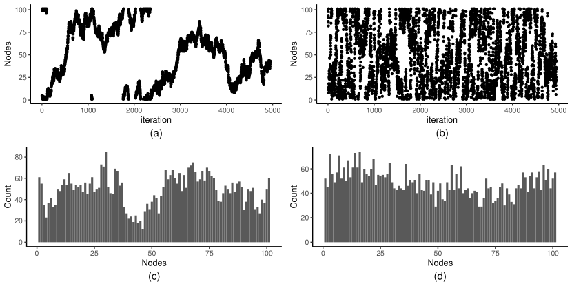
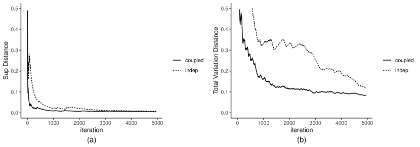
Refer to caption
Figure 2: Scatter plot (top) and histogram (bottom) of the target chain on the circulant graph C1011superscriptsubscript𝐶1011C_{101}^{1}. Plot (a) and (c) represent the behavior of the target chain for the case in which two chains are independent whereas plot (b) and (d) show the behavior of the target chain for the case in which two chains are Metropolis-coupled.
Refer to caption
Figure 3: Plots of distance changes of the target chains on the circulant graph C1011superscriptsubscript𝐶1011C_{101}^{1} : the left one represents the convergence of Lsubscript𝐿L_{\infty} distance and the right one shows the convergence of total variation distance. The solid lines represent the distance change of the coupled target chain, and the dotted lines stand for the distance change of the independent target chain.
Refer to caption
Figure 4: Scatter plot (top) and histogram (bottom) of the target chain on the circulant graph C1001,2,3superscriptsubscript𝐶100123C_{100}^{1,2,3}. Plot (a) and (c) represent the behavior of the target chain for the case in which two chains are independent whereas plot (b) and (d) show the behavior of the target chain for the case in which two chains are Metropolis-coupled.
Refer to caption
Figure 5: Plots of distance changes of the target chains on the circulant graph C1001,2,3superscriptsubscript𝐶100123C_{100}^{1,2,3} : the left one represents the convergence of Lsubscript𝐿L_{\infty} distance and the right one shows the convergence of total variation distance. The solid lines represent the distance change of the coupled target chain, and the dotted lines stand for the distance change of the independent target chain.
Refer to caption
Figure 6: Scatter plot (top) and histogram (bottom) of the target chain on the random 3-regular graph. Plot (a) and (c) represent the behavior of the target chain for the case in which two chains are independent whereas plot (b) and (d) show the behavior of the target chain for the case in which two chains are Metropolis-coupled.
Refer to caption
Figure 7: Plots of distance changes of the target chains on the random 3-regular graph : the left one represents the convergence of Lsubscript𝐿L_{\infty} distance and the right one shows the convergence of total variation distance. The solid lines represent the distance change of the coupled target chain, and the dotted lines stand for the distance change of the independent target chain.
Refer to caption
Figure 8: Scatter plot (top) and histogram (bottom) of the target chain on the Watts–Strogatz model. Plot (a) and (c) represent the behavior of the target chain for the case in which two chains are independent whereas plot (b) and (d) show the behavior of the target chain for the case in which two chains are Metropolis-coupled.
Refer to caption
Figure 9: Plots of distance changes of the target chains on the Watts-Strogatz model : the left one represents the convergence of Lsubscript𝐿L_{\infty} distance and the right one shows the convergence of total variation distance. The solid lines represent the distance change of the coupled target chain, and the dotted lines stand for the distance change of the independent target chain.