Information flow in parameterized quantum circuits

Abstract

In this work, we introduce a new way to quantify information flow in quantum systems, especially for parameterized quantum circuits. We use a graph representation of the circuits and propose a new distance metric using the mutual information between gate nodes. We then present an optimization procedure for variational algorithms using paths based on the distance measure. We explore the features of the algorithm by means of the variational quantum eigensolver, in which we compute the ground state energies of the Heisenberg model. In addition, we employ the method to solve a binary classification problem using variational quantum classification. From numerical simulations, we show that our method can be successfully used for optimizing the parameterized quantum circuits primarily used in near-term algorithms. We further note that information-flow based paths can be used to improve convergence of existing stochastic gradient based methods.

I Introduction

Parameterized quantum circuits (PQCs) are a central component of many variational quantum algorithms (VQAs) with applications in quantum chemistry and combinatorial optimization [1, 2, 3], such as the Variational Quantum Eigensolver [4] and the Quantum Approximate Optimization Algorithm [5]. In addition, variational algorithms have more recently been applied to a number of machine learning tasks, including data classification [6, 7, 8] and generative modeling [9, 10, 11, 12, 13, 14]. The general concept behind VQAs is to employ a PQC to generate a trial wavefunction on a quantum device. The resulting state is then repeatedly measured to estimate expectation values of some Hermitian operator(s) using the current trial wavefunction. These expectation values are used to evaluate an objective function that a classical optimizer maximizes or minimizes by varying the parameter values of the PQC.

In recent years, significant progress has been made to better understand PQCs, their design, and their relationship to algorithm performance. For example, expressibility and entanglement capability have been proposed as meaningful metrics to compare different PQCs and exclude circuits with limited capabilities [15]. Moreover, expressibility has been correlated with other performance metrics of certain variational quantum algorithms [16], and high expressibility has been associated with the presence of barren plateaus in cost function landscapes [17]. However, there is still a general lack of understanding of how the parameterization of quantum circuits impacts algorithm performance.

In this work, we propose a novel method to characterize the information flow in PQCs to incorporate correlations between parameters in a quantum circuit. To quantify the information flow, we first consider a graph representation of quantum circuits to define paths between the two-qubit unitaries present in the quantum circuit. We then introduce a measure of distance between two points in a circuit by mapping local unitaries into a multi-qubit state and using mutual information between the resulting single-qubit states. Finally, using the distance metric, we propose a new method for stochastic optimization of variational algorithms using a subset of gate parameters from a selected (random or shortest) path.

We perform numerical simulations to analyze the performance of the proposed method for two different tasks; ground state energy estimation and binary classification. Applying our method for optimization of VQAs, we observe that using (shortest) paths consistently outperforms the stochastic gradient-based method.

The rest of the paper is organized as follows: we present some preliminary information required to understand the article in section II, and details of the method used in the article are presented in section III. Next, the results from numerical simulations is presented in section IV and we finally present some concluding remarks in section V.

II Preliminaries

II.1 Mutual Information

For a bipartite quantum system on two subsystems $A$ and $B$, the state space can be represented as the tensor product of the individual sub-spaces as: $\mathcal{H}^{AB}=\mathcal{H}^{A}\otimes\mathcal{H}^{B}$. The quantum mutual information $I(A:B)$ is a measure of the amount of correlation between the two sub-systems and is defined as:

$$I(A:B)=S(\rho^{A})+S(\rho^{B})-S(\rho^{AB}),$$ (1)

where $\rho^{AB}$ represents the density matrix of the full system on $\mathcal{H}^{AB}$, $\rho^{A}=\Tr_{B}(\rho^{AB})$ and $\rho^{B}=\Tr_{A}(\rho^{AB})$ are the reduced state of $\rho^{AB}$ on systems $A$ and $B$ respectively, and $S(\rho)=-\Tr(\rho\log\rho)$ represents the von Neumann entropy of a density matrix $\rho$.

II.2 Quantum Circuits as Graphs

A quantum circuit is a sequence of operations that can be used to prepare a state of interest on a quantum device. It typically comprises of simple unitary operations called quantum gates that depend on some parameters. The action of the circuit $U(\theta)$ on an initial state $\ket{\psi_{0}}$ prepares the state $\ket{\psi(\theta)}=U(\theta)\ket{\psi_{0}}$.

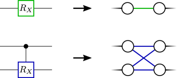
We develop a simple strategy for converting a quantum circuit into a directed graph by representing every quantum gate as edges in the graph and the states at different moments in the circuits as nodes. Using this picture, a single qubit gate is represented as an edge that connects two nodes, while a two-qubit gate is represented as four edges between four nodes. The nodes are then arranged as per the time steps in the quantum circuit. The open edges represent the initial state and the resulting state of the qubits. 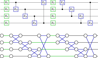A simple illustration of this conversion is shown in Fig. 1.

(a) An illustration of the graph representation of single and two qubit gates.

(b) An illustration of the graph representation of the full circuit.

Figure 1: A figure showing the graph representation of a given circuit.

II.3 Information Flow

Information flow is defined as the transfer of information from one variable to another in a process. In the context of quantum circuits, this can be regarded as the spread of correlation between qubits as a result of multi-qubit gates. Analogously one can think of it as the spread of correlation between gates in their corresponding causal cones. The spread of correlation has been considered in previous studies [18, 19] to design better ansatz for variational algorithms.

In this work, we use the notion of information flow (spread of correlation) to define paths through the circuit, using which we can control the spread of correlation between qubits. We combine the concept of causal cones with paths and utilize the graph representation of a parameterized quantum circuit to identify and control the flow of information (correlation) between gates. An illustration of these concepts is depicted in Fig. 2.

Figure 2: A figure showing the causal cone and the various paths in a graph representation of a circuit. The nodes present in the causal cone of the observable on qubit 4 are colored blue, and the color gradient represent the distance (darker implies smaller). The blue lines denote different paths within the causal cone.

II.4 Optimization of variational quantum algorithms

In variational quantum algorithms we usually optimize the parameters of states prepared by a PQC, $U(\theta)$, in order to minimize an objective function of the form:

$$f(\theta)=\langle H\rangle_{\theta}=\sum_{j=1}^{M}\langle H_{j}\rangle_{\theta}$$ (2)

where $H$ represent a problem Hamiltonian, which is a linear combination on $M$ Pauli terms $H_{j}$. The optimization of the objective function is carried out by iteratively updating the parameters of the quantum circuit as:

$$\mathbf{\theta}^{(t+1)}_{i}=\mathbf{\theta}^{(t)}_{i}-\alpha\frac{\partial f(\mathbf{\theta})}{\partial\mathbf{\theta}_{i}},$$ (3)

where $\alpha$ is the learning rate and $\frac{\partial f(\mathbf{\theta})}{\partial\mathbf{\theta}_{i}}$ denotes the partial derivative of the objective function with respect to the variable $\mathbf{\theta}_{i}$. The analytical gradient can be calculated using a K-term parameter-shift rule [20, 21, 22, 23] as:

$$\frac{\partial f(\mathbf{\theta})}{\partial\mathbf{\theta}_{i}}=\sum_{j=1}^{M}\frac{\partial\langle H_{j}\rangle_{\theta}}{\partial\mathbf{\theta}_{i}}=\sum_{j=1}^{M}\sum_{k=1}^{K}\gamma_{k,i}\langle H_{j}\rangle_{\theta_{k,i}},$$ (4)

where, $\gamma_{k,i}$ is the $K-$term coefficient in the shift rule. The calculation of the analytical gradient requires a large number of measurements for a single parameter update, as every gradient calculation requires $K$ objective evaluations, which in turn requires a large number of measurements (shots) for accurate estimation of each objective. To overcome this, $n$-shot stochastic gradient descent was proposed in Ref. [24, 25] where one uses $n$-shot estimators of the gradient instead of the exact ones,

$$\frac{\partial f(\mathbf{\theta})}{\partial\mathbf{\theta}_{i}}=\sum_{j=1}^{M}\sum_{k=1}^{K}\gamma_{k,i}\tilde{h}_{j}^{(n)}({\theta_{k,i}}),$$ (5)

where, $\tilde{h}_{j}^{(n)}({\theta_{k,i}})$ is the $n$-sample mean estimator of $\langle H_{j}\rangle_{\theta_{k,i}}$. The parameter are then updated similarly to equation 3.

II.5 Variational Quantum Classification

Variational quantum classifiers (VQC) are quantum circuits that are trained for supervised learning tasks [7, 8]. There exist several strategies to design a quantum classifier, including well-known classical machine learning techniques such as artificial neural networks [26, 27] or kernel methods [28, 29].

Figure 3: Structure of an $n$-qubit variational quantum binary classifier: state preparation circuit $E(\bm{x})$ encoding the input $\bm{x}$ into the amplitudes of a quantum system, a model circuit $U(\theta)$, and a single qubit measurement. The measurement retrieves the probability $p(y)$ of the model predicting 0 or 1, from which the binary prediction can be inferred. The classification circuit parameters $\theta$ are trained by a variational scheme.

In this study, the circuit-centric architecture in Fig. 3 is used to study a binary classification problem [8]. The general objective is to train the VQC on a data set $\{\bm{x}_{i},y_{i}\}_{train}$ to find a mapping between input $\bm{x}_{i}$ and label $y_{i}$. The trained parameterized quantum circuit can then be used as a black box to predict labels $\hat{y}_{i}$ for a given set of test inputs $\{\bm{x}_{i},y_{i}\}_{test}$.

The circuit used for this classification task consists of three distinct parts: The state preparation circuit, the model circuit, and a measurement scheme. Preparing a quantum state that embeds some classical data is achieved by applying a static quantum routine on the initial ground state $\ket{\Phi(x)}=E(x)\ket{0}$. Using the so-called basis encoding method

$$\ket{\Phi(x)}=\bigotimes_{i=0}^{n}\ket{x_{i}},$$ (6)

with $x\in\mathbb{B}^{n}$ , encodes the input data $\bm{x}$ as computational basis states. The prepared state $\ket{\Phi(x)}$ is then further processed with a given parametrized quantum circuit $U(\theta)$ resulting in a state $\ket{\psi_{vqc}(\bm{x},\theta)}=U(\theta)E(\bm{x})\ket{0}$. The ansatz structure used in this study contains parameterized single and two-qubit gates with trainable parameters. The circuit is shown in Fig. 4. The output state $\ket{\psi_{vqc}(\bm{x},\theta)}$ is finally measured using the Pauli-Z operator on a qubit (we chose the first qubit) and obtaining the expectation value $\mathbb{E}(\sigma_{z})$. This yields the predicted label $(\hat{y}_{i})$.

Figure 4: Gate composition of a single layer of the ansatz used in the model circuit $U(\theta)$ for the classification task.

The parameters of the variational block are trained by minimizing the square loss cost function

$$f(\theta) =\frac{1}{n^{\prime}}\sum_{i=0}^{n^{\prime}}\left(y_{i}-\hat{y}_{i}(\theta)\right)^{2}$$ (7)

with $n^{\prime}$ as the training set size and the predicted label output of the VQC as

$$\hat{y}_{i}(\theta) =\bra{\psi(x_{i},\theta)}\sigma_{z}\otimes\mathbb{I}^{\otimes n-1}\ket{\psi(x_{i},\theta)}.$$ (8)

The binary classification problem studied in this paper is the $n$-bit parity problem. The corresponding dataset contains $2^{n}$ distinct binary vectors, where each label indicates whether the sum of the $n$ components of the binary vector is odd or even. The Boolean $n$-bit parity function to be modeled is

$$f:\{0,1\}^{\otimes n}\xrightarrow{}\{0,1\},$$ (9)

with the property that $f(x)=1$ if the number of ones in the vector $x\in\{0,1\}^{n}$ is odd or zero otherwise.

In what follows, we describe the details of how to quantify information flow for designing algorithm to optimize variatonal algorithms.

III Method

III.1 Measure of distance

A given unitary $\hat{U}$ on two qubits can be conveniently described using a $4\times 4$ matrix $U_{(a,b),(c,d)}$ with entries:

$$U_{(a,b),(c,d)} =\left<c,d\right|\hat{U}\left|a,b\right> a,b,c,d\in\{0,1\}\;,$$ (10)

where the indices $(a,b)$ are thought of as a single unified row-index, and $(c,d)$ similarly plays the role of a unified column-index. Using this description, a four qubit state corresponding to the unitary transformation can be defined:

$$\left|\psi_{U}\right> =\frac{1}{\mathcal{N}}\sum_{a,b,c,d\,\in\,\{0,1\}}U_{(a,b),(c,d)}\left|a,b,c,d\right>\;,$$ (11)

where, $\mathcal{N}$ is a normalization-constant.

Using this state, we can now define reduced density matrices of different subsystems of qubits. For instance, we can define the single- and two-qubit reduced density-matrices:

$$\rho^{a} =\text{Tr}_{\{b,c,d\}}\left(\left|\psi_{U}\right>\left<\psi_{U}\right|\right)$$

$$\rho^{ab} =\text{Tr}_{\{c,d\}}\left(\left|\psi_{U}\right>\left<\psi_{U}\right|\right)\;,$$

where the subscripts on the trace indicates the degrees of freedom that are traced over.

Using this description of the unitary Ref. [30] proposed the following distance metric across the legs of the unitary (see Fig. 5):

$$d_{i,j} =-\log\left(\frac{I(i:j)}{2\log\left(2\right)}\right)\;,$$ (12)

where, $I(i:j)$ is the mutual information between the sites $i$ and $j$ as defined in Eq. 1.

Figure 5: An illustration of the definition of labels on the unitary operator, as well as the corresponding labeling of the metric distances. Image adapted from Ref. [30].

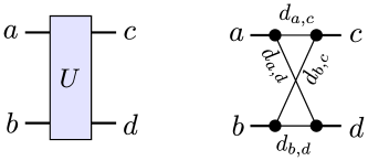
In this article we introduce a further modification to the distance metric as:

$$\tilde{d}_{i,j}=\begin{cases}-\log\left(\frac{I(i:j)}{4\log\left(2\right)}\right)\quad\text{if }(i,j)\in\{(a,c),(b,d)\}\\ \\ -\log\left(\frac{I(ac:bd)}{4\log\left(2\right)}\right)\quad\text{else}\end{cases}$$ (13)

where, $I(ij:kl)$ is defined as:

$$I(ij:kl) =S\left(\rho^{ij}\right)+S\left(\rho^{kl}\right)-S\left(\rho^{ijkl}\right)$$

$$=S\left(\rho^{ij}\right)+S\left(\rho^{kl}\right)$$ (14)

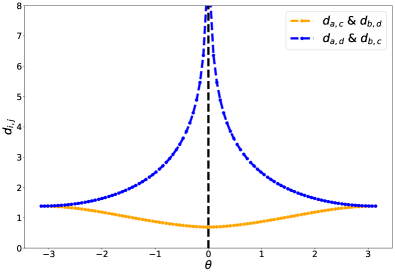
To develop some intuition about this metric, we present an illustration of the distance between the legs of a two qubit gate, C-Ry($\theta$), in Fig. 6. As expected, we observe that the distance (weight of the diagonal edges) approaches infinity when theta equals zero because the two qubit gate at this value acts as identity.

Figure 6: A plot of the distance vs. the parameter value for a C-Ry($\theta$) gate.

Figure 7: A figure showing the different path options in the causal cone of an observable. The intensity of the colors (darker implies smaller) denote the qualitative distance from the last point on the qubit to measured.

III.2 Paths

The objective functions $f(\theta)$ for commonly used quantum algorithms are constructed as a linear combination of expectation values as:

$$f(\theta)=\sum_{j=1}^{M}\langle H_{j}\rangle_{\theta},$$ (15)

where $H_{j}$ represent individual Pauli-strings in the Hamiltonian defining the problem. These individual Pauli-strings usually acts on the state of a subset of the full qubits, and their expectation value thus depends on the gate parameter in the causal cone of these qubits.  [31] We define different paths in the causal cone of the qubits to be measured by converting the quantum circuits into graphs as described in section II.2. An illustration of the choices of paths in the causal cone is shown in Fig. 7.

We further introduce the notion of shortest paths by adding weights to the edges in the graph representation of the circuit according to the distance measure proposed in section III.1. This is inspired from Ref. [30] where the authors use the length of geodesics for disentangling a quantum state. We use the networkx package [32] to create the graph representation of the quantum circuit and for finding different paths between nodes in the graph representation.

III.3 Optimization with paths

In this section, we present a strategy for optimizing variational algorithms based on paths in the causal cone of the individual Pauli-strings used to define the objective function. We use two different strategies of choosing sets of parameters by randomly sampling paths from either the set of all possible paths or the set of shortest paths. The overall algorithm is presented in Algorithm 1.

Input: choice of path, problem Hamiltonian and ansatz

Output: Ground state energy of the Hamiltonian

Initialize: generate the circuit graph

while not converged do

       for term in Hamiltonian do

             select a path based on the distance metric and the sampling strategy

            

       end for

      

      for path in all paths do

             1. select the parameters in the path

             2. calculate the gradients w.r.t. every parameter using Eq. 4

             3. update the parameters using the gradients and learning rate using Eq. 3

            

       end for

      

end while

Algorithm 1 An outline of the path optimization algorithm.

One can also modify the presented algorithm to add more stochasticity by randomly sampling the Hamiltonian terms to optimize in each step [33, 25] or by updating parameters before calculating paths for terms. We leave these variations for future studies.

IV Simulation and Results

In this section, we numerically demonstrate the applications of the proposed algorithm for training variational quantum algorithms. The training is implemented in Tequila [34] an open-source python package which uses Qulacs [35] as the backend for the execution of all the numerical simulations. We also used the Pennylane [36] package for running some of the numerical simulations. We first present the details of the experiments for finding ground state energies.

IV.1 VQE - XXZ-Heisenberg model

We use the VQE framework to find the ground state energy of the XXZ-Heisenberg model. The Hamiltonian of such a system can be written as follows:

$$\hat{H}=\sum_{\langle i,j\rangle}\left(-J_{X}\hat{X}_{i}\hat{X}_{j}-J_{Y}\hat{Y}_{i}\hat{Y}_{j}-J_{Z}\hat{Z}_{i}\hat{Z}_{j}\right)-h\sum_{k}\hat{Z}_{k}$$ (16)

where $\hat{X},\hat{Y},\hat{Z}$ are the Pauli matrices, $\langle i,j\rangle$ denotes all the pairs of adjacent lattice sites, and $J_{X},J_{Y},J_{Z}$ are the coupling constant and $h$ on the right represents the external magnetic field. The coupling constants for the XXZ-model follow the relation: $J=J_{X}=J_{Y}\neq J_{Z}\equiv\Delta$. For all the experiments, we fix the values of the different constants to $h=0$ (no external magnetic field), $\Delta=-20.0$ and $J=1.0$. This corresponds to the model having a ferromagnetic ground state. We use this model due to the fact that all the terms in the Hamiltonian depend on only the state of two qubits, e.g. $\hat{X}_{i}\otimes\hat{X}_{j}$, and thus our method can be very useful in reducing the cost of parameter updates in every iteration of the optimization.

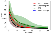
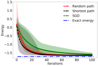
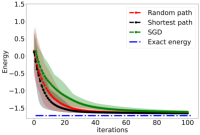
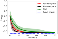
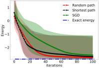
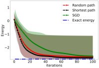
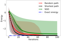
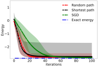
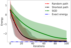
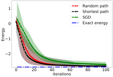
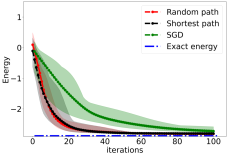
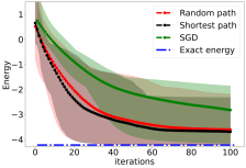
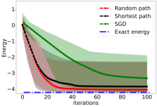
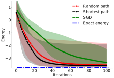
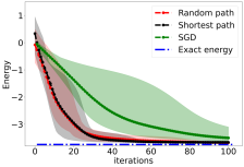
We carried out simulations for five different lattice sizes, starting with $3\times 2$ qubits, $4\times 2$ qubits, $5\times 2$ qubits, $6\times 2$ qubits and $7\times 2$ qubits (6, 8, 10, 12, and 14 qubits respectively). For all the simulations we use the ansatz shown in Fig. 1(b) with varying number of layers. The optimization is carried out using the algorithm presented in Algorithm 1 and the stochastic gradient descent algorithm, with a fixed learning rate of $0.1$. The results from all the simulations are plotted in Figure 8. We only plot the first 100 iterations of the trajectories for all the cases, as it is sufficient for comparing the different methods. All the simulations were repeated at least 5 times with random initialization of the gate parameters to collect the statistics for comparison.

We look at the optimization trajectories from the different simulations using a single layer of the ansatz plotted in Fig. 8. First, we observe that optimization using Algorithm 1 with either a random or shortest path always performs better when compared with stochastic gradient descent. Second, we observe that the optimization trajectories using the shortest path on average have steeper initial convergence, however, the final energies achieved by all optimization methods were very close. This indicates that choosing a set of parameters based on information transfer between qubits via gates can help accelerate the overall convergence of an algorithm. Also, it should be noted that forcing the flow of information along a particular path can be useful in cases where the spread of information can lead to convergence issues. [37] Finally, we point out that the spread in the trajectories corresponding to the runs with the shortest path tends to be smaller, however, all the methods have some runs (particularly in the case of the 12 qubit model) where they converge to a local minimum. This is a common occurrence in stochastic optimization methods and can be mitigated using different methods. [38]

As we increase the number of layers of the ansatz used in the numerical simulations, we observe that the rate of convergence for all the methods increases. However, we point out that optimization trajectories with the shortest path are still the fastest converging among all the methods. This implies that using (shortest) paths for optimization of algorithms with objectives depending on only a subset of the qubits might be useful.

1. 6 Qubit Ansatz
a) 1 layer	b) 2 layers	c) 3 layers	d) 4 layers
2. 8 Qubit Ansatz
a) 1 layer	b) 2 layers	c) 3 layers	d) 4 layers

3. 10 Qubit Ansatz
a) 1 layer	b) 2 layers	c) 3 layers

4. 12 Qubit Ansatz
a) 1 layer	b) 2 layers
5. 14 Qubit Ansatz
a) 1 layer	b) 2 layers

Figure 8: Optimization trajectories from different VQE simulations of the different XXZ-Hamiltonians. The lines correspond to the mean of the trajectories from different runs, and the shadow represent the area between the best and worst values from the simulations.

IV.2 VQC - Binary classification

We use the VQC framework presented in Section II.5 for the $n$-bit parity classification problem. The corresponding dataset of such a system consists of $2^{n}$ distinct binary vectors, where each label indicates whether the sum of the $n$ components of the binary vector is odd or even. The Boolean $n$-bit parity function to be modeled is

$$f:\{0,1\}^{\otimes n}\xrightarrow{}\{0,1\}$$ (17)

with the property that $f(x)=1$ if the number of ones in the vector $x\in\{0,1\}^{n}$ is odd. Binary classification is an interesting choice for this study because there is only one readout qubit, making the problem well-suited for our optimization method.

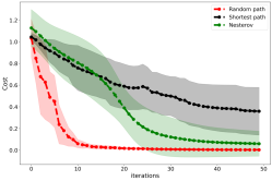
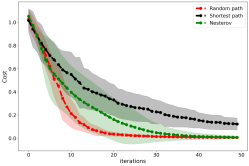
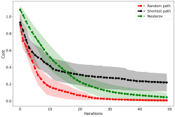
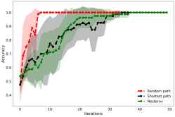
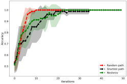
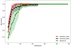
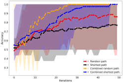
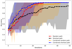
Simulations were performed on the 4-qubit parity problem using the ansatz shown in Fig. 4 with $2,3,$ and $4$ layers. Again, optimization is performed using the algorithm presented in Algorithm 1 and Nesterov momentum with a fixed learning rate of 0.1. We selected the Nesterov optimizer for comparison, as using Adam failed to improve the model accuracies. The simulation results are shown in Fig. 9. We focus on the first 50 training epochs of optimization for all cases and plot the average of 5 instances with random initialization of the gate parameters to collect statistics for comparison.

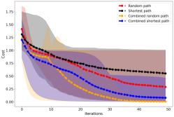
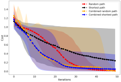
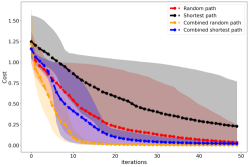
As can be seen from the optimization trajectories in Fig. 9, the model is able to learn to successfully perform the classification task. We note that the optimization with random paths consistently outperforms the one with the Nesterov momentum method. However, we observe that the optimization with the shortest path performs poorly. We attribute this to the fact that the model has limited knowledge of the full data to compute the parity at any given step. So to test this hypothesis and inform the model of the full input state, we perform numerical simulations with paths to all qubits instead of a single random path. The combined paths in the worst case can correspond to the causal cone of the observable, which has been considered for optimization in previous works. [31] Furthermore we carry out the simulation with the paths alongside the combined paths with a reduced learning rate of 0.05 and plot the results in Fig. 10. The reason for training with a reduced learning rate is that we observe oscillations in the cost function with the combined paths.

Cost function
a) 2 Layers	b) 3 Layers	c) 4 Layers
Accuracy of the model
a) 2 Layers	b) 3 Layers	c) 4 Layers

Figure 9: Optimization trajectories from different VQC simulations of the n-bit parity problem using a 4-qubit ansatz. The lines correspond to the mean of the trajectories from different runs, and the shadow represents one standard deviation.

Cost function
a) 2 Layers	b) 3 Layers	c) 4 Layers
Accuracy of the model
a) 2 Layers	b) 3 Layers	c) 4 Layers

Figure 10: Optimization trajectories from different VQC simulations of the n-bit parity problem using a 4-qubit ansatz with a reduced learning rate. The lines correspond to the mean of the trajectories from different runs, and the shadow represents the area between the best and worst values from the simulations.

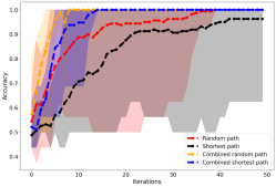We note that the trajectories from the optimization with the combined paths outperform the optimization with individual paths consistently. This is the expected behavior as the model has access to the full data for the classification as compared to the case with individual paths. We further point out that the optimization with the random path on average has a higher convergence rate as compared to the one with the shortest path. This can be due to the fact that it can have access to a larger number of parameters as compared to the shortest path. While this suggests that one needs larger number of parameters here, we point that we can still find the optimal solution using single paths which only depend on a subset of the parameters.

Overall, we have presented empirical evidence that our method based on the path (defined using a distance measure) can be used to successfully optimize variational algorithms.

V Conclusion

In this work, we have proposed a notion of information flow by defining a path in parameterized quantum circuits. We have presented a novel measure of distance between two points in the circuit by using mutual information between the quantum states that a local unitary acts on. The distance can be calculated efficiently as it does not rely on global parameters but only on the local unitary operator. We also present a strategy for optimizing parameterized circuits using paths for variational quantum algorithms.

We performed numerical experiments to estimate the ground state energy of the XXZ-Heisenberg model as well as do n-bit binary classification, using parameterized circuits of varying size and depth. The results from the numerical simulations provide empirical evidence that our method can be successfully used for these tasks.

Our work is an initial step toward using path-based information flow for the optimization of quantum circuits. While we have demonstrated consistent improvement for smaller problem instances, a systematic investigation of the scaling of our method for sufficiently deep circuits could be worth exploring. Other questions such as if forcing information along paths can help mitigate the observed barren plateau phenomenon or remove redundant parameterization of quantum circuits are left for future research. We believe that results from this study can be useful to researchers studying the optimization and design of quantum circuits.

References

- Bharti et al. [2022] K. Bharti, A. Cervera-Lierta, T. H. Kyaw, T. Haug, S. Alperin-Lea, A. Anand, M. Degroote, H. Heimonen, J. S. Kottmann, T. Menke, et al., Reviews of Modern Physics 94, 015004 (2022).
- Cerezo et al. [2021] M. Cerezo, A. Arrasmith, R. Babbush, S. C. Benjamin, S. Endo, K. Fujii, J. R. McClean, K. Mitarai, X. Yuan, L. Cincio, et al., Nature Reviews Physics 3, 625 (2021).
- Anand et al. [2022] A. Anand, P. Schleich, S. Alperin-Lea, P. W. Jensen, S. Sim, M. Díaz-Tinoco, J. S. Kottmann, M. Degroote, A. F. Izmaylov, and A. Aspuru-Guzik, Chemical Society Reviews (2022).
- Peruzzo et al. [2014] A. Peruzzo, J. McClean, P. Shadbolt, M.-H. Yung, X.-Q. Zhou, P. J. Love, A. Aspuru-Guzik, and J. L. O’Brien, Nature Communications 5, 4213 (2014).
- Farhi et al. [2014] E. Farhi, J. Goldstone, and S. Gutmann, A quantum approximate optimization algorithm (2014).
- Havlíček et al. [2019a] V. Havlíček, A. D. Córcoles, K. Temme, A. W. Harrow, A. Kandala, J. M. Chow, and J. M. Gambetta, Nature 567, 209 (2019a).
- Farhi and Neven [2018a] E. Farhi and H. Neven, Classification with quantum neural networks on near term processors (2018a).
- Schuld et al. [2020] M. Schuld, A. Bocharov, K. M. Svore, and N. Wiebe, Physical Review A 101, 10.1103/physreva.101.032308 (2020).
- Romero and Aspuru-Guzik [2019] J. Romero and A. Aspuru-Guzik, Variational quantum generators: Generative adversarial quantum machine learning for continuous distributions (2019).
- Zhu et al. [2019] D. Zhu, N. M. Linke, M. Benedetti, K. A. Landsman, N. H. Nguyen, C. H. Alderete, A. Perdomo-Ortiz, N. Korda, A. Garfoot, C. Brecque, L. Egan, O. Perdomo, and C. Monroe, Science Advances 5, eaaw9918 (2019), https://www.science.org/doi/pdf/10.1126/sciadv.aaw9918 .
- Situ et al. [2020] H. Situ, Z. He, Y. Wang, L. Li, and S. Zheng, Information Sciences 538, 193 (2020).
- Zeng et al. [2019] J. Zeng, Y. Wu, J.-G. Liu, L. Wang, and J. Hu, Phys. Rev. A 99, 052306 (2019).
- Lloyd and Weedbrook [2018] S. Lloyd and C. Weedbrook, Phys. Rev. Lett. 121, 040502 (2018).
- Dallaire-Demers and Killoran [2018] P.-L. Dallaire-Demers and N. Killoran, Phys. Rev. A 98, 012324 (2018).
- Sim et al. [2019] S. Sim, P. D. Johnson, and A. Aspuru-Guzik, Advanced Quantum Technologies 2, 1900070 (2019).
- Hubregtsen et al. [2020] T. Hubregtsen, J. Pichlmeier, P. Stecher, and K. Bertels, Evaluation of parameterized quantum circuits: on the relation between classification accuracy, expressibility and entangling capability (2020).
- Holmes et al. [2022] Z. Holmes, K. Sharma, M. Cerezo, and P. J. Coles, PRX Quantum 3, 10.1103/prxquantum.3.010313 (2022).
- Zhang et al. [2021a] Z.-J. Zhang, T. H. Kyaw, J. S. Kottmann, M. Degroote, and A. Aspuru-Guzik, Quantum Science and Technology 6, 035001 (2021a).
- Zhang et al. [2021b] Y. Zhang, L. Cincio, C. F. Negre, P. Czarnik, P. Coles, P. M. Anisimov, S. M. Mniszewski, S. Tretiak, and P. A. Dub, arXiv preprint arXiv:2106.07619 (2021b).
- Schuld et al. [2019] M. Schuld, V. Bergholm, C. Gogolin, J. Izaac, and N. Killoran, Physical Review A 99, 032331 (2019).
- Mari et al. [2021] A. Mari, T. R. Bromley, and N. Killoran, Physical Review A 103, 012405 (2021).
- Kottmann et al. [2021a] J. S. Kottmann, A. Anand, and A. Aspuru-Guzik, Chemical science 12, 3497 (2021a).
- Wierichs et al. [2022] D. Wierichs, J. Izaac, C. Wang, and C. Y.-Y. Lin, Quantum 6, 677 (2022).
- Harrow and Napp [2021] A. W. Harrow and J. C. Napp, Physical Review Letters 126, 140502 (2021).
- Sweke et al. [2020] R. Sweke, F. Wilde, J. Meyer, M. Schuld, P. K. Fährmann, B. Meynard-Piganeau, and J. Eisert, Quantum 4, 314 (2020).
- McClean et al. [2018] J. R. McClean, S. Boixo, V. N. Smelyanskiy, R. Babbush, and H. Neven, Nature Communications 9, 4812 (2018).
- Farhi and Neven [2018b] E. Farhi and H. Neven, Classification with quantum neural networks on near term processors (2018b).
- Schuld and Killoran [2019] M. Schuld and N. Killoran, Phys. Rev. Lett. 122, 040504 (2019).
- Havlíček et al. [2019b] V. Havlíček, A. D. Córcoles, K. Temme, A. W. Harrow, A. Kandala, J. M. Chow, and J. M. Gambetta, Nature 567, 209 (2019b).
- Hyatt et al. [2017] K. Hyatt, J. R. Garrison, and B. Bauer, Physical review letters 119, 140502 (2017).
- Benedetti et al. [2021] M. Benedetti, M. Fiorentini, and M. Lubasch, Physical Review Research 3, 033083 (2021).
- Hagberg et al. [2008] A. Hagberg, P. Swart, and D. S Chult, Exploring network structure, dynamics, and function using NetworkX, Tech. Rep. (Los Alamos National Lab.(LANL), Los Alamos, NM (United States), 2008).
- Kivlichan et al. [2019] I. D. Kivlichan, C. E. Granade, and N. Wiebe, arXiv preprint arXiv:1907.10070 (2019).
- Kottmann et al. [2021b] J. Kottmann, S. Alperin-Lea, T. Tamayo-Mendoza, A. Cervera-Lierta, C. Lavigne, T.-C. Yen, V. Verteletskyi, P. Schleich, A. Anand, M. Degroote, S. Chaney, M. Kesibi, N. G. Curnow, B. Solo, G. Tsilimigkounakis, C. Zendejas-Morales, A. F. Izmaylov, and A. Aspuru-Guzik, Quantum Science and Technology (2021b).
- Suzuki et al. [2021] Y. Suzuki, Y. Kawase, Y. Masumura, Y. Hiraga, M. Nakadai, J. Chen, K. M. Nakanishi, K. Mitarai, R. Imai, S. Tamiya, et al., Quantum 5, 559 (2021).
- Bergholm et al. [2018] V. Bergholm, J. Izaac, M. Schuld, C. Gogolin, M. S. Alam, S. Ahmed, J. M. Arrazola, C. Blank, A. Delgado, S. Jahangiri, et al., arXiv preprint arXiv:1811.04968 (2018).
- Marrero et al. [2021] C. O. Marrero, M. Kieferová, and N. Wiebe, PRX Quantum 2, 040316 (2021).
- Swenson et al. [2020] B. Swenson, R. Murray, S. Kar, and H. V. Poor, arXiv preprint arXiv:2003.02818 (2020).
- Ponce et al. [2019] M. Ponce, R. van Zon, S. Northrup, D. Gruner, J. Chen, F. Ertinaz, A. Fedoseev, L. Groer, F. Mao, B. C. Mundim, et al., in Proceedings of the Practice and Experience in Advanced Research Computing on Rise of the Machines (learning) (2019) pp. 1–8.
- Loken et al. [2010] C. Loken, D. Gruner, L. Groer, R. Peltier, N. Bunn, M. Craig, T. Henriques, J. Dempsey, C.-H. Yu, J. Chen, et al., in Journal of Physics-Conference Series, Vol. 256 (2010) p. 012026.