STI: Turbocharge NLP Inference at the Edge via Elastic Pipelining

Abstract.

Natural Language Processing (NLP) inference is seeing increasing adoption by mobile applications, where on-device inference is desirable for crucially preserving user data privacy and avoiding network roundtrips. Yet, the unprecedented size of an NLP model stresses both latency and memory, creating a tension between the two key resources of a mobile device. To meet a target latency, holding the whole model in memory launches execution as soon as possible but increases one app’s memory footprints by several times, limiting its benefits to only a few inferences before being recycled by mobile memory management. On the other hand, loading the model from storage on demand incurs IO as long as a few seconds, far exceeding the delay range satisfying to a user; pipelining layerwise model loading and execution does not hide IO either, due to the high skewness between IO and computation delays.

To this end, we propose Speedy Transformer Inference (STI). Built on the key idea of maximizing IO/compute resource utilization on the most important parts of a model, STI reconciles the latency v.s. memory tension via two novel techniques. First, model sharding. STI manages model parameters as independently tunable shards, and profiles their importance to accuracy. Second, elastic pipeline planning with a preload buffer. STI instantiates an IO/compute pipeline and uses a small buffer for preload shards to bootstrap execution without stalling at early stages; it judiciously selects, tunes, and assembles shards per their importance for resource-elastic execution, maximizing inference accuracy.

Atop two commodity SoCs, we build STI and evaluate it against a wide range of NLP tasks, under a practical range of target latencies, and on both CPU and GPU. We demonstrate that STI delivers high accuracies with 1–2 orders of magnitude lower memory, outperforming competitive baselines.

Figure 1. Comparison of model execution methods. Our method achieves high accuracy at low memory cost. T: target latency. M: model memory for Transformer weights.

1. Introduction

Natural Language Processing (NLP) is seeing increasing adoption by mobile applications (de Barcelos Silva et al., 2020). For instance, a note-taking app allows users to verbally query for old notes and dictate new notes. Under the hood, the app invokes an NLP model in order to infer on user input. It is often desirable to execute NLP inference on device, which crucially preserves user data privacy and eliminates long network trips to the cloud (Tambe et al., 2021; Cartas et al., 2019).

NLP inference stresses mobile devices on two aspects. (1) Impromptu user engagements. Each engagement comprises a few turns (Bogers et al., 2019); users expect short delays of no more than several hundred ms each turn (Carrascal and Church, 2015), often mandated as target latencies (Tambe et al., 2021). (2) Large model size. Designed to be over-parameterized (Michel et al., 2019; Yu et al., 2020), today’s NLP models are hundred MBs each (Devlin et al., 2019; Sanh et al., 2019; Radford et al., 2019), much larger than most vision models (Sandler et al., 2018; Zhang et al., 2018). As a common practice, separate NLP model instances are fine-tuned for tasks and topics, e.g. one instance for sentiment classification (ber, 2022) and one for sequence tagging (Bhattacharjee et al., 2020), which further increase the total parameter size on a mobile device.

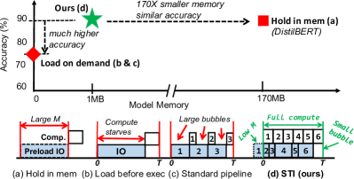
How to execute NLP models? There are a few common approaches (Figure 1). (1) Hold in memory: preloading a model before user engagement or making the model linger in memory after engagement. The efficacy is limited: a model in memory increases one app’s memory footprint (often less than 100MB (Lebeck et al., 2020; Lee and Bahn, 2021)) by a few times, making the app a highly likely victim of the mobile OS’s low memory killer (Android, 2022); as user engagements are bursty and each consists of as few as 1-3 model executions (Bogers et al., 2019), a lingering model likely benefits no more than 2 executions before its large memory is reclaimed by the OS; since user engagements are impromptu (Li et al., 2015; Tian et al., 2020), predicting when to preload/unload models is challenging. (2) Load on demand. The problem is the long IO delays for loading a NLP model. For instance, DistilBERT, a popular model optimized for mobile, takes 2.1 seconds to load its 170 MB parameters as we measured, far exceeding user desirable latencies of several hundred ms. To hide IO delays, one may stream model parameters from storage to memory during computation: execute model layer $k$ while loading parameters for layer $k+1$. While such an IO/compute pipeline was known in ML (Yi et al., 2022; Miao and Lin, 2021), directly applying it to NLP inference is ineffective: the core parts of NLP models such as attention has a skewed IO/compute ratio due to low arithmetic intensity (Wang, 2020). As a result, most of the time (¿72%) the computation is stalling.

These approaches suffer from common drawbacks: (1) key resources – memory for preload and IO/compute for model execution – are managed in isolation and lack coordination; (2) obliviousness to a model’s parameter importance, i.e. which parameters matter more to model accuracy. Hence, the preload buffer unnecessarily holds parameters that could have been streamed in parallel to execution; IO unnecessarily loads parameters that the computation cannot consume within the target latency. The results are memory waste, frequent pipeline stalls, and inferior model accuracy due to low FLOPs.

Our design

We present an engine called STI. Addressing the drawbacks above, STI integrates on-demand model loading with lightweight preload, getting the best of both approaches.

(1) A model as resource-elastic shards. The engine preprocesses an N-layer model: partitioning each layer into $M$ shards; compressing each shard as $K$ fidelity versions, each version with a different parameter bitwidth. The engine therefore stores the $N\times M\times K$ shard versions on flash. At run time, the engine assembles a submodel of its choice: a subset of $n$ layers ($n<=N$); $m$ shards ($m<=M$) from each selected layer; a fidelity version for each selected shard. Any such submodel can yield meaningful inference results, albeit with different accuracies and resource costs. Our model sharding is a new combination of existing ML techniques (Hou et al., 2020; Zadeh et al., 2020).

In this way, the engine can dynamically vary a model’s total execution time, adjust IO/compute ratios for individual shards, and allocate IO bandwidth by prioritizing important shards.

(2) Preload shards for warming up pipeline. The engine maintains a small buffer of preload shards, adjusting the size to available memory. Instead of trying to hold the entire model, it selectively holds shards from a model’s bottom layers (closer to input). Upon user engagement, the engine can start executing the early stage of a pipeline with much of the parameters already loaded, which otherwise would have to stall for IO.

(3) A joint planner for memory, IO, and computation. The engine’s planner selects shards and their versions to preload and to execute. Its goal is to compose a submodel that simultaneously meets the target latency, minimizes pipeline stalling, and maximizes accuracy.

Towards this goal, our ideas are (1) set layerwise IO budgets according to layerwise computation delays and (2) allocate IO budgets according to shard importance. To plan, STI first decides a submodel that can be computed under the target latency. The engine then sets accumulated IO budgets (AIBs) at each layer to be the computation delays of all prior layers; it further treats the available memory for preload shards as bonus IO budgets to all layers. Having set the budgets, the engine iterates over all shards, allocating extra bitwidths to loading important shards and hence debiting IO budgets of respective layers. The engine preloads the first $k$ shards in the layer order that maximize the usage of preload memory size $|S|$ but not exceeding $|S|$.

Results

We implement STI atop PyTorch and demonstrate it on mobile CPU and GPU of two embedded platforms. On a diverse set of NLP tasks, STI meets target latencies of a few hundred ms while yielding accuracy comparable to the state of the art. We compare STI against competitive baselines enhanced with recent ML techniques (Hou et al., 2020; Zadeh et al., 2020) as illustrated in Figure 1. Compared to holding a model in memory, STI reduces parameter memory by 1-2 orders of magnitude to 1–5MB, while only seeing accuracy drop of no more than 0.1 percentage points; compared to existing execution pipelines, STI increases accuracy by 5.9-54.1 percentage points as its elastic pipeline maximizes both compute and IO utilization.

Contributions

The paper makes the following contributions:

• Model sharding, allowing the engine to fine control an NLP model’s total computation time and finetune each shard’s IO time according to resource constraints and shard importance.

• A pipeline with high IO/compute utilization: a small preload buffer for warming up the pipeline; elastic IO and computation jointly tuned to minimize pipeline bubbles and maximize model accuracy.

• A two-stage planner for the pipeline: picking a submodel, tracking layerwise IO budgets, and prioritizing importance shards in resource allocation.

2. Motivations

2.1. Transformer on Mobile Devices

A primer on transformer

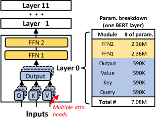
Figure 2 shows the architecture of Transformer (Vaswani et al., 2017), the modern NN developed for NLP tasks. Compared with traditional NNs (e.g. LSTM (Hochreiter and Schmidhuber, 1997)), it features a unique Multi-Headed Attention (MHA) mechanism. MHA extracts features at sequence dimension by modeling pairwise word interactions through many attention heads (typically 12), which are backed by three fully-connected (i.e. linear) layers, namely Query (Q), Key (K), Value (V). Given an input, each attention head independently contributes an attention score as one representation of the feature space. Scores across attention heads are concatenated via a linear output layer (O) and then projected into higher feature dimensions by two linear layers in the point-wise Feed-Forward Network (FFN) module.

Due to the large number of fully connected layers, a transformer based model contains over 100 million parameters. As a result, a typical pretrained model is of a few hundred MBs. For instance, BERT (Devlin et al., 2019) as one of the most popular model is over 400MB large.

Figure 2. (Left) The BERT model comprising transformer layers and (Right) the number of 32-bit floating point parameters within a layer (Vaswani et al., 2017).

Resource demands

(1) Low latencies. Prior studies show that users expect mobile devices to respond in several hundred milliseconds, and their satisfaction quickly drops as latency grows beyond around 400ms (Chen et al., 2019). (2) Large model parameters. The scale of NLP parameters is unprecedented for on-device machine learning. Even DistilBERT (Sanh et al., 2019) optimized for mobile has nearly 200MB of parameters, contrasting to popular vision models which are as small as a few MBs (Sandler et al., 2018; Zhang et al., 2018). Such numerous parameters stress both memory capacity and IO for loading them.

Besides parameters, model execution also allocates memory for intermediate results. Yet, such data has short lifespans and does entail loading from storage. Hence, it can be served with a relatively small working buffer sufficient to hold a model tile (often a few MBs); the size does not grow with the model size. We therefore do not optimize for it.

2.2. Transformers Challenge Existing Paradigms

Existing paradigms are inadequate, as shown in Figure 1.

First, hold in memory.

An app may keep model files lingering in memory or even pin them; thus, the model can start execution anytime without IO delays. For how long the app holds the model depends on its prediction of future user engagements.

The major drawback is that an in-memory model will take hundreds of MBs of memory, bloating an app’s memory footprint which is often less than 100 MBs (Lebeck et al., 2020; Lee and Bahn, 2021). When an app’s memory footprint is much larger than its peers, it becomes a highly likely victim of mobile memory management, which aggressively kills memory-hungry apps (Lebeck et al., 2020). Once killed, the app has to reload the model for the next engagement. Furthermore, precise prediction of user engagement is difficult, as mobile apps often exhibit sporadic and ad hoc usage (Shepard et al., 2011; Carrascal and Church, 2015). To exacerbate the problem, co-running apps may invoke separate models for their respective tasks, e.g. for sentiment analysis and for next-word prediction.

Second, load before execute.

As the default approach by popular ML frameworks (pyt, 2022; ten, 2022): upon user engagement, the app sequentially loads the model and executes it. As we measured on a modern hexa-core Arm board (see Table 2), it takes 3.6 seconds to execute DistilBERT, among which 3.1 seconds are for loading the whole 240 MB model file. Prior work observed similar symptoms of slow start of model inference (Yang et al., 2020; Yi et al., 2022).

Third, pipelined load/execution.

To hide IO delays, one may leverage layerwise execution of ML models (Huang et al., 2019; Narayanan et al., 2019) and overlap the layer loading IO and execution (Yi et al., 2022; Miao and Lin, 2021). This approach is barely effective for on-device NLP due to the high skewness between IO delays and computation delays. As we measured, a layer in DistilBERT requires 339 ms for parameter load while only 95 ms to compute. The root causes are (1) low arithmetic intensity in Transformer’s attention modules (Pati et al., 2021) and (2) mobile device’s efficiency-optimized flash, which limits the rate of streaming parameters from storage to memory. As a result, the pipeline is filled with bubbles and the computation stalls most of the time at each model layer.

Section 7 will compare our system against these approaches.

2.3. Model Compression Is Inadequate

For efficient NLP inference, a popular category of techniques is model compression, including pruning networks (e.g. layers (Sanh et al., 2019) and attention heads (Voita et al., 2019)), reducing feature dimensions (Sun et al., 2020), and sharing weights across layers (Lan et al., 2020). A notable example is DistilBERT (Sanh et al., 2019): through distilling knowledge, it prunes half of BERT’s layers, shrinking the model by $2\times$.

Still, model compression alone is inadequate. (1) While one may compress a model to be sufficiently small (e.g. $\sim$10MBs (Qin et al., 2022)) so that the load delay or the memory footprint is no longer a concern, the resultant accuracy is inferior, often unusable (Tay et al., 2020). (2) The execution pipeline’s bubbles still exist: compression often scales model compute and parameters in tandem, without correcting the computation/IO skewness. Hence, compute is still being wasted. (3) Most compression schemes lack flexibility as needed to accommodate diverse mobile CPU, GPU, and IO speeds. They either fix a compression ratio or require model re-training to adjust the ratios, which must done by the cloud for each mobile device.

Section 7 will evaluate the impact of model compression.

3. Design overview

3.1. The System Model

STI incarnates as a library linked to individual apps. For complete NLP experience, we assume that the app incorporates other components such as automatic speech recognition (ASR), word embedding, and speech synthesis (Shi et al., 2021; Wilkening et al., 2021; Wan et al., 2021; Eisenman et al., 2019). As they often run much faster than model execution and are orthogonal to STI, this paper does not optimize for them.

STI loads and executes a model by layer: it loads one layer (comprising multiple shards) as a single IO job, decompresses all the shards in memory, and computes with the layer as a single compute job. IO and compute jobs of different layers can overlap. STI does not use smaller grains (e.g. load/execute each shard) as they leave the IO and GPU bandwidth underutilized, resulting in inferior performance.

STI allocates two types of memory buffers.

• Preload buffer holds shards preloaded selectively. STI keeps the buffer as long as the app is alive. STI can dynamically change the buffer size as demanded by the app or the OS.

• Working buffer holds a layer’s worth of intermediate results and uncompressed parameters. The buffer is temporary, allocated before each execution and freed afterward. The buffer size is largely constant, not growing with the model size; it is not a focus of STI.

Figure 3. System architecture of Speedy Transformer Inference (STI) and workflow.

3.2. The Operation

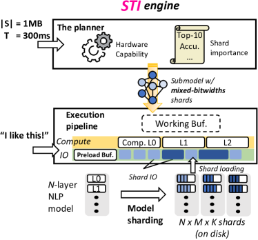
The STI architecture is shown in Figure 3. STI preprocesses a given language model (e.g. DistilBERT finetuned for sentiment analysis): decomposing the model into shards and profiling shard importance (Section 5). As a one-time, per-model effort, the preprocessing is expected to be done in the cloud prior to model deployment to mobile devices; as preprocessing only requires lightweight model transformation (as opposed to expensive re-training (Liu et al., 2019)), it can be done on device as needed. The resultant model shards are stored alongside apps.

STI profiles each device’s hardware once. The goal is to measure IO and computation delays in executing a language model; the profiling results serve as the basis for pipeline planning. To do so, STI loads and executes a Transformer layer in different bitwidths.

As an app launches, STI is initialized as part of the app. The app specifies which NLP model(s) it expects to execute, as well as the corresponding target latencies $T$s and preload buffer sizes $|S|$s. Later, the app can update $T$s and $|S|$s at any time. For each expected model, STI plans a separate execution pipeline with separate preload model shards. STI plans a pipeline once and executes it repeatedly. Replanning is necessary only when a model’s $T$ or $|S|$ is changed by the app or OS.

Upon user engagement, STI executes a pipeline for the requested model. Since planning is already done beforehand, STI simply loads and executes the shards that have been selected in planning.

3.3. Example Execution Scenarios

One-shot execution

In this scenario, a user engagement consists of one turn, executing the model once. With preloaded shards, STI executes the pipeline without stalling in bottom layers, which are close to input. STI uses the working buffer during the execution and frees it right after. Throughout the execution, the content of preload buffer is unchanged.

A few back-to-back executions

One engagement may comprise multiple executions (often no more than 3) (Bogers et al., 2019). The scenario is similar to the above, except for the opportunity of caching already loaded shards between executions. To this end, the app may request to enlarge the preload buffer so it selectively caches the loaded shards. In subsequent executions, STI no longer reloads these shards; its planner redistributes the freed IO bandwidth to other shards (Section 5), loading their higher-fidelity versions for better accuracy. After the series of executions, the app may choose to keep the additional cached shards as permitted by the OS or simply discard them.

3.4. Applicability

STI supports Transformer-based models (Wang et al., 2020; Hou et al., 2020; Liu et al., 2019). This paper focuses on classification tasks (BERT and its variants), which underpin today’s on-device NLP. Although STI’s key ideas apply to generative models such as GPT-2 (Radford et al., 2019), their wide adoption on mobile (in lieu of template-based responses (McTear et al., 2016)) is yet to be seen; we consider them as future work.

STI keeps a model’s execution time under a target latency $T$. However, it alone is insufficient to keep the total wall-clock time under $T$. Such a guarantee would require additional OS support, e.g. real-time scheduling. STI lays the foundation for such a guarantee.

STI expects a small preload buffer. It can, however, work without such a buffer (i.e. “cold start” every time), for which its elastic sharding and pipeline still offer significant benefits as we will show in Section 7.

On future hardware/workloads, we expect STI’s benefit to be more pronounced: mobile compute continues to scale (due to advances in technology nodes and accelerators); users expect results in higher accuracy; NLP models are becoming larger. All these lead to higher computation/IO skewness, necessitating an elastic pipeline of loading and execution.

4. Elastic model sharding

4.1. Key Challenges

We solve a key challenge: how to partition the model into individual shards? Set to enable the resource elasticity of a model (i.e. depths/widths/fidelity), the shards must meet the following criteria:

• Elastic execution. Shards must preserve the same expressiveness of the attention mechanism and can execute partially to produce meaningful results.

• Tunable IO. The IO delays of shards must be tunable to accommodate IO/compute capability of different hardware (e.g. due to diverse CPU/GPUs and DVFS).

4.2. Instantiating Model Shards on Disk

To address the challenges, our key idea is to combine two machine learning techniques – dynamic transformer (Hou et al., 2020; Wang et al., 2020) and dictionary-based quantization (Han et al., 2016), in a novel way. We next describe details.

Figure 4. Instantiating $N\times M\times K$ model shards on disk. The example shows a 2-bit shard. 99.9% of its weights are represented by 2-bit indexes pointing to $2^{2}$ centroids; the rest 0.1% outliers are preserved as-is.

First, vertical partitioning per layer

The system adopts a pretrained transformer model, which has already been fine-tuned on a downstream task.

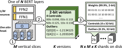
For each of the $N$ layers, the system partitions it into $M$ vertical slices, as shown in Figure 4 ( ). By construction, each vertical slice is independent, constituting one attention head plus $1/M$ of FFN neurons of the layer; the partitioning is inspired by dynamic transformers (Wang et al., 2020; Hou et al., 2020). Table 1 shows the weight compositions of a vertical slice. Each cell of the table describes the dimension of the weight matrix, where $d$ is the hidden state size, $M$ is the number of attention heads, and $d_{ff}$ is the number of FFN neurons; a shard is therefore one of the $M$ equal slices of a layer. Doing so warrants model shards the same capability to extract linguistic features from inputs, as done by the attention mechanism: of an individual shard, its attention head obtains one independent representation of input tokens, which is projected into a higher feature dimension by FFN neurons (Voita et al., 2019; Clark et al., 2019); jointly, multiple shards attend to information from different representation subspace at different positions (Vaswani et al., 2017). Therefore, an arbitrary subset of shards of a layer can be executed and still give meaningful results.

STI uses the submodel to describe the transformer model on shards, e.g. a $n\times m$ submodel comprises $n$ layers, each layer having $m$ shards. The number $m$ is the same across all layers, as mandated by the transformer architecture (Vaswani et al., 2017), which specifies each layer must have the same width (i.e. number of shards $m$) for aligning input/output features between layers. Although it is possible for a shard to use 0s as dummy weights, STI expects all $m$ shards to have concrete weights for a good accuracy.

Table 1. The weight composition of a shard. $M$ is number of attention heads. The $M$ shards equally slices a transformer layer, where each shard of the layer can be uniquely identified by its vertical slice index $i=0\dots M-1$.

	Attn (Q,K,V,O)	FFN1	FFN2
Transformer Layer	$d\times d$	$d_{ff}\times d$	$d\times d_{ff}$
Shard (vertical slice)	$d\times\frac{d}{M}$	$\frac{d_{ff}}{M}\times d$	$d\times\frac{d_{ff}}{M}$

Second, quantization per shard

The system compresses each of the $N\times M$ shards into $K$ bitwidths versions (e.g. $K=2\dots 6$). STI is the first to bring quantization to shard granularity, whereas prior work only explores layer granularity (Gong et al., 2019; Dong et al., 2019; Wang et al., 2019). Doing so reduces IO/compute skewness and facilitates elastic IO, allowing STI to prioritize IO resources at a much finer granularity, e.g. by allocating higher bitwidths to more important shards, and catering to IO/compute capability of diverse devices.

To compress, STI uses Gaussian outlier-aware quantization (Zadeh et al., 2020). The key idea is to represent the vast majority of weights (e.g. 99.9%) which follow a Gaussin distribution using $2^{k}$ floating point numbers (i.e. centroids); doing so compresses the original 32-bit weights into $k$-bit indexes pointing to centroids, thus reducing the parameter size by $\frac{32}{k}$. For the very few outliers (e.g. 0.1%) which do not follow the Gaussian distribution, it preserves their weights as-is. The process is shown in Figure 4 ( ). We will further describe the implementation details in Section 6.

We choose it for two main reasons. 1) It provides good compatibility between shards of different bitwidths, allowing STI to tune their bitwidth individually per their importance and to assemble a mixed-bitwidth submodel. This is due to its lossy compression nature – shards still preserve the original distribution of layer weights, albeit in different fidelities. Hence they can work with each other seamlessly. 2) It does not need to fine-tune a model or require additional hardware support. The quantization analyzes the weight distribution of the pretrained model and is not specific to network structures; it hence does not require fine-tuning, as opposed to fixed-point quantization (Zafrir et al., 2019; Qin et al., 2022). The resultant mixed-bitwidth submodel also differs from a traditional mixed-precision network (Wang et al., 2019; Dong et al., 2019; Gong et al., 2019), which requires DSP extensions for executing integer operations efficiently; the extensions are often exclusive to microcontrollers on ARM devices, e.g. Cortex-M4 (Lorenser, 2016).

Quantized shards are not meant to be used as-is. Prior to use, STI must decompress them, which is a mirror process of compression. STI does so by substituting dictionary indexes with floating point centroids and outliers. Therefore model shards quantization reduces IO but not computation (FLOPs) as the inference still executes on floating point numbers.

Third, storing shards per version

STI stores each shard of every bitwidth on disk, in total $N\times M\times K$ shards (e.g. N=M=12, K=$2\dots 6,32$, where 32 is the uncompressed, full fidelity). Each shard contains a weight matrix of the same dimensions listed in Table 1. Instead of original FP32 weights, the weight matrix now stores K-bit indexes, which reduces its file size by $32/K\times$. Additional to the weight matrix, it stores centroids and outliers as dictionaries to look up during decompression, as illustrated by Figure 4 ( ). To load, it refers to individual on-disk shards by their original layer/vertical slice indexes and bitwidths.

5. Pipeline planning

5.1. Overview

Planning goals

Towards maximizing the accuracy under a target latency T, STI plans for two goals:

• First, minimize pipeline bubbles. STI attempts to utilize both IO and computation as much as possible: by keeping IO always busy, it loads higher-bitwidth shards to improve submodel fidelity; by maxing out computation (FLOPs), it drives the inference towards a higher accuracy.

• Second, prioritize bitwidths on important shards. As transformer parameters exhibit clear redundancy, STI allocates IO bandwidths with respect to shard importance, i.e. a shard is more important if it contributes more significantly to accuracy when being executed in higher bitwidths.

Two-stage planning

Towards the goals, STI conducts a two-stage planning: 1) Compute planning. Based on measured computation delay of a layer, it proposes the largest submodel R’ bound by T, which has the maximum FLOPs. 2) IO planning. It first assigns an accumulated IO budget (AIB) to each layer of the submodel R’ for tracking layerwise IO resources. To allocate and saturate the IO resources, STI attempts to consume each layer’s AIB. Starting from most important shards, STI assigns them a higher bitwidth, e.g. 6-bit; it does so iteratively for less important shards, until no AIB is left for each layer. We next describe details.

5.2. Prerequisite: Offline Profiling

The following measurements are done ahead of time, off the inference execution path.

Hardware capability

STI measures the following hardware capabilities of a mobile device at installation time.

• IO delay $T_{io}(k)$ as a function of bitwidth $k$. STI measures the average disk access delay for loading one shard in $k$ bitwidth, where $k=2\dots 6,32$. It only has to measure one shard per bitwidth because all others have same amount of parameters.

• Computation delay $T_{comp}(l,m,\textit{freq})$ as a function of $l$, the input sentence length, $m$, the number of shards per layer (e.g. $m=3\dots 12$), and freq as the current operating frequency of CPU/GPU. It fixes $l$ to be commonly used input lengths after padding (e.g. $l=128$). It does a dry run for each $(l,m,\textit{freq})$ tuple on one transformer layer. It measures the average execution delay as the decompression delay of $m$ shards in 6-bitwidth and the execution delay of the transformer layer composed by the $m$ shards. Although the decompression delay is strictly dependent on the shard bitwidth, the delay differences between individual bitwidths are negligible in practice, e.g. $<1ms$; measuring 6-bitwidth shards further bounds the decompression delays, ensuring STI always stays under the target latency.

The delays can be recorded offline and replayed at run time because they are data-independent (Guo and Lin, 2022; Park and Lin, 2021) and are shown deterministic (Wang et al., 2021), w.r.t. the parameters $k,l,m,\text{and}\ \textit{freq}$.

Shard importance

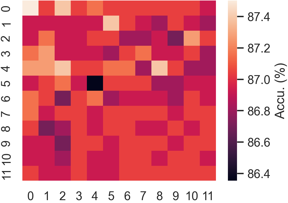
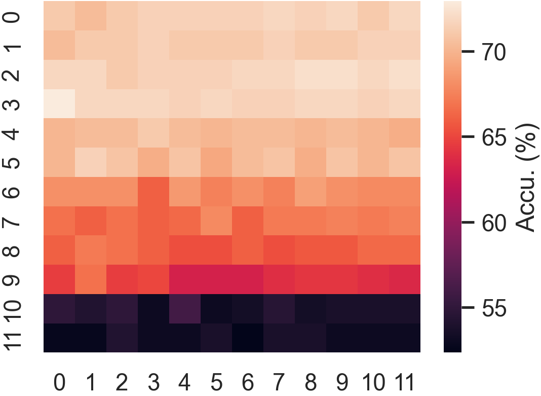
Intuitively, important shards have greater impacts on accuracy. Formally, STI deems a shard more important than another if the shard increases the model accuracy more significantly as they have higher fidelities. Specifically, STI profiles shard importance as follows. It first sets the full 12x12 model (i.e. with 144 shards) to the lowest bitwidth (i.e. 2-bit), enumerates through each shard, and increases the shard bitwidth to the highest (i.e. 32-bit); for each enumeration, it runs the resultant model on a dev set and profiles its accuracy. The profiling therefore produces a table (e.g. with $12\times 12=144$ entries), whose each entry records the model accuracy when the individual shard is at the highest bitwidth while all others are at the lowest bitwidth. STI then sorts the table by model accuracy and obtains the list of ranked shard importance.

Notably, the profiling needs to be done for individual fine-tuned models, which have different weight distributions. Figure 5 and 5 shows the example of profiling results for models used in SST-2 and RTE respectively. As can be seen, shards of different models exemplify dissimilar importance distributions. For instance, important shards distribute more evenly throughout the layers of SST-2 model yet they are much more concentrated on bottom layers (i.e. layer 0-5) of RTE model.

(a) SST-2

(b) RTE

Figure 5. Example shard profiles on SST-2 and RTE show distinct importance distribution. Each cell at (x, y) marks a shard; the lighter its color is, the more important the shard is (i.e. the higher accuracy during profiling). Y-axis: transformer layer index, X-axis: vertical slice index.

5.3. Compute Planning

Given a target latency T, STI proposes a submodel sized by $n\times m$ for the incoming inference, which maximizes FLOPs.

Key ideas

In searching for the submodel size, STI follows two principles: 1) whenever possible, it always picks the submodel with most number of shards, i.e. $n\times m$ is maximized; 2) when two candidate submodels have similar number of shards, it prefers the deeper one, i.e. the candidate with a larger $n$. As the transformer attention heads within the same layer are known to be redundant (Michel et al., 2019), it is wiser to incorporate more layers.

To infer $(n,m)$, STI enumerates through all possible pairs using the profiled $T_{comp}(l,m,freq)$; the enumeration process has a constant complexity and is efficient. Since all inputs can be padded to a constant length (e.g. $l=128$), and $freq$ is often at peak during active inference, STI only needs to enumerate in total 144 pairs in practice. For each T, the enumeration therefore deterministically gives a submodel of $(n\times m)$ which is both largest and deepest.

5.4. IO Planning

In this stage, STI selects the bitwidths for individual shards of the $(n\times m)$ submodel. Without stalling the pipeline, it seeks those that maximize accuracy.

5.4.1. Problem Formulation

Given the deadline $T$, $n\times m$ submodel $R$ determined by compute planning, and the preload buffer $S$, STI plans for a shard configuration $S^{\prime}$ to load during computation, s.t. 1) loading $S^{\prime}$ does not stall the pipeline, and 2) $R=S+S^{\prime}$ achieves maximum accuracy.

5.4.2. Accumulated IO Budgets

To ensure the planning $S^{\prime}$ does not stall the pipline, STI uses Accumulated IO Budgets (AIBs) to track fine-grained, per-layer available IO bandwidth.

Key ideas

To quantify AIBs, our observation is that the pipeline does not stall iff before executing one layer, all shards of the current and prior layers are already loaded. We hence define AIBs as follows:

Definition 0 (Accumulated IO Budgets).

The AIB(k) of $k^{th}$ layer is the available IO time the layer can leverage to load all shards from $0\dots k$ layers, written as $AIB(k)=AIB(k-1)+T_{comp}(k-1)$, where $T_{comp}(k-1)$ is the computation delay of the $(k-1)^{th}$ layer.

The recursive definition (i.e. hence accumulated) encodes the data dependency between pipeline layers: each layer crucially depends on previous layers’ available IO budgets and computation delays for overlapping the loading of its own shards. As of the very first layer, its AIB is set as the IO delay to fill the preload buffer $S$, considered as “bonus IO”. For instance, the AIB of the second layer is the AIB plus the computation delay of the first layer, i.e. $AIB(1)=AIB(0)+T_{comp}(0)$. With the above definition, STI checks AIBs of all layers: as long as they are non-negative, STI knows each layer still has IO time remaining and the pipeline does not stall, and deems the planning valid.

How to use

Upon each planning, STI initializes AIBs for all layers as follows. It first sets AIB(0) to be the IO delay to fill the preload buffer as described before. Next, STI sets subsequent AIBs recursively using the above definition, e.g. $AIB(1)=AIB(0)+T_{comp},AIB(2)=AIB(0)+2\times T_{comp},AIB(3)=AIB(0)+3\times T_{comp}$. Note that since layers have an identical structure, STI uses a constant $T_{comp}$ across all layers.

When STI selects a shard at $k$-th layer, it deducts the shard IO from AIBs of $k$-th as well as all subsequent layers. This is because loading such shards only affect yet-to-be-executed layers but not the already executed ones. At the end of selection, STI checks all AIBs to see if they are non-negative. If so, STI deems the planning $S^{\prime}$ valid, otherwise rejects it.

Figure 6. A mini example of AIB tracking the layerwise IO budgets.

Example

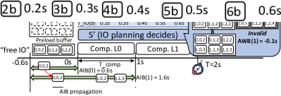
Figure 6 shows a mini example of using AIBs to check the validity of $S^{\prime}$, where it plans for a 2x3 submodel, targeting a 2s deadline with $T_{comp}=1s$. The engine initializes AIBs recursively from L0, whose $AIB(0)=0.6s$ due to the three 2-bit shards in $S$. To plan, the engine first fills $S^{\prime}$ with $S$, deducting $0.6s$ from both $AIB(0)$ and $AIB(1)$ because all shards in $S$ are in L0. Since only L1 has spare AIB, the engine can only select shards for it. We show three execution plan candidates A, B, and C. In this case, both candidates A and B are valid because their AIBs are non-negative, meaning loading them does not stall computation L1. Yet, C is invalid, because $AIB(1)=-0.1s$, violating the constraint and stalling the pipeline.

5.4.3. Selecting Optimal Shard Versions

For each $T$, there exist an enormous number of execution plans. The goal is to select an optimal configuration $S^{\prime}$, which 1) is valid, and 2) maximizes accuracy. For instance, both A and B in Figure 6 are valid, but which has the maximum accuracy?

Key idea

To ensure validity, STI respects the key invariant $AIB(k)\geq 0$ for each allocation attempt on layer $k$. To maximize accuracy, our key idea is to first uniformly increase bitwidths for all shards, then with the rest AIBs it greedily and iteratively allocates highest possible bitwidths to individual shards guided by shard importance. By doing so, we build an information passageway for most important shards, allowing their maximum activations to be preserved in as high fidelity as possible.

The allocation process comprises two passes as follows. In the first pass, STI picks a uniform bitwidth for all unallocated shards in the submodel, i.e. those not in preload buffer. To do so, it enumerates from lowest bitwidth (i.e. 2-bit) and selects the highest bitwidths while AIBs still satisfy the invariant. Notably, it fills a submodel layer with the shards from the same original layer and does not mix up shards across layers, due to quantization preserves intra-layer weight distribution (§4.2). If AIBs cannot even support 2-bit shards, e.g. due to $T$ and/or preload buffer $S$ too small, STI still selects them as they are necessary for execution but aborts further allocation. In the second pass, STI iteratively upgrades the bitwidths of individual shards to full 32 bitwidth guided by the shard importance profiled in §5.2, until all AIBs are consumed.

The allocation result is an optimal execution plan which instantiates the submodel with individual shard configurations, and is ready to be executed by the IO/compute pipeline.

5.5. Submodel Execution

STI executes the plan (i.e. the $n\times m$ submodel with selected shards) in a layerwise, pipelined manner from layer 0 to layer n-1. While conceptually it is possible to pipeline shard computation within the same layer, STI does not do so due to limited benefits – within a layer there exists data dependency between the FFNs and attention module.

STI executes both IO and computation as fast as possible; it does not reorder the loading of individual shards in order to meet data dependency between execution, because by design AIBs have already ensured so. To compute, STI decompresses the shards into the working buffer using the dictionaries stored along with them; the working buffer is enough to hold one layer of FP32 weights and shared by all layers during their ongoing execution. After execution, STI evicts loaded shards from top to bottom layers until preload buffer is filled. It does so because shards at bottom layers (i.e. closer to input) are needed early during inference. Preserving as many of them as possible avoids compulsory pipeline stalls in early stages.

6. Implementation

We implement STI in 1K SLOC (Python: 800, C: 200) based on PyTorch v1.11 (tor, 2022) and sklearn v0.23.2 (skl, 2022), atop two commodity SoCs listed in Table 2.

We preprocess the pretrained DynaBERT (Hou et al., 2020) models. We choose them because they are easily accessible and well documented. We preprocess the model as follows. To quantize a model into k bitwidth, we first partition the model by layers and gathers all weights of the layer into a large flat 1D array. We then fit the 1D array into a Gaussian distribution using GaussianMixture with one mixture component from sklearn.mixture for detecting outliers. Based on the fitted distribution, we calculate the log likelihood of each sample in the 1D weight array. Following (Zadeh et al., 2020) we also use -4 as the threshold – if the weight’s log likelihood is below the threshold, we deem it as an outlier and records its array index; in our experiments, a model only has 0.14-0.17% outliers, which are an extremely small portion. For non-outliers which are the vast majority, we sort them based on their values and divided them into $2^{k}$ clusters with equal population. We calculate the arithmetic mean of each cluster as one centroid for representing all weights of the cluster. With such, we extract shards from the layer based on their weight composition in Table 1 and massively substitutes their weights with k-bit indexes to centroids; for bit alignment, we represent outliers also as k-bit integers but bookkeep their original weights and offsets in the shard. We repeat the process for each layer and for each $k=2\dots 6$, which takes a few minutes per bitwidth. We co-locate disk blocks of shards from the same layer for access locality. To measure shard importance, we use dev set from the respective GLUE benchmark on which the model is fine-tuned.

Implementing the layerwise pipeline is straightforward, by intercepting the forwarding function at each BERT layer and using asynchronous IO for loading shards. Yet, we have discovered Python has a poor support for controlling concurrency at fine granularity (e.g. via low-level thread abstraction), which introduces artificial delays to shard decompression. Therefore we implement the decompression in separate 200 SLOC of C code using OpenMP (Dagum and Menon, 1998), which concurrently substitutes the low-bit integers back to FP32 centroids using all available cores of our SoCs; we expect the decompression to be further accelerated with GPU, but leave it as future work.

For miscellaneous parameters of a layer which are not part of shards, i.e. layer normalization (layernorm) and biases, we keep them in memory in full fidelity because their sizes are small, e.g. tens of KB per layer.

Table 2. Platforms in evaluation. Benchmarks run on Odroid’s CPU (its GPU lacks Pytorch support) and Jetson’s GPU.

7. Evaluation

We answer the following questions:

1. Can STI achieve competitive accuracy under time and memory constraints? (§7.2)

2. How much do STI’s key designs contribute to its performance? (§7.3)

3. How do STI’s benefits change with available time and memory? (§7.4)

7.1. Methodology

Setup and metrics

Table 2 summarizes our test platforms, which are commodity SoCs. We choose them to evaluate STI on both CPU and GPU. Based on user satisfaction of NLP inference delays on mobile devices (Chen et al., 2019), we set T=150, 200, and 400ms. Prior work reported that beyond 400ms user satisfaction greatly drops (Chen et al., 2019). With T under 100ms, all comparisons including STI show low accuracy – there is not enough compute bandwidth. This is a limit in our test hardware, which shall mitigate on faster CPU/GPU.

Table 3 summarizes our benchmarks and metrics. We diversify them to include each category of GLUE benchmarks (Wang et al., 2018), which span a broad range of NLP use cases on mobile devices.

Table 3. GLUE benchmarks (Wang et al., 2018) used in evaluation.

Comparisons

We consider two NLP models. (1) DistilBERT (Sanh et al., 2019), the outcome of knowledge distillation from BERT. Due to its high popularity on mobile, we use its accuracy as our references and call it gold accuracy. Yet, DistilBERT has fixed depths/widths (6 layers x 12 heads) and thus cannot adapt to different target latencies. (2) DynaBERT (Hou et al., 2020), which is derived from BERT (12 layers x 12 heads), allowing execution of a submodel to meet the target latency.

Based on DynaBERT, we design the following competitive baselines as summarized in Table 4.

Table 4. Baselines for evaluation and their positions in the design space.

• Load&Exec: It loads model as a whole and executes it. It chooses the best submodel so the sum of IO and execution delays is closest to the target latency, using the algorithm described in Section 5.3. Model parameters are not quantized (32 bits).

• Standard pipelining (StdPL-X): It executes a layerwise pipeline, overlapping IO and computation. It chooses the best submodel so that the total pipeline delay stays under the target latency. We further augment it with quantization. All parameters in a model have the same bitwidth X.

• PreloadModel-X: The whole model is already in memory and no IO is required. It chooses the best submodel so that the total computation delay stays under the target latency. We augment it with quantization; all parameters have the same bitwidth X.

We choose X=6 as the highest quantization bitwidth, as further increasing the bitwidth has little accuracy improvement.

Table 5. Model execution accuracies; given target latencies, ours are the best or the closest to the best. —S—: preload buffer size. Gold accuracy from DistilBERT (Sanh et al., 2019), which exceed all target latencies. End-to-end DistilBERT execution delays: 3.7s on Odroid, of which IO=3.1s; 3.36s on Jetson, of which IO=3.0s.

7.2. End-to-End Results

STI achieves comparable accuracies to gold under target latencies (T) of a few hundred ms. Across all benchmarks and latencies, STI accuracy is on average 7.1 percentage point (pp) higher than that of baselines, which is significant.

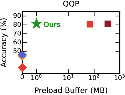
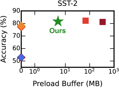
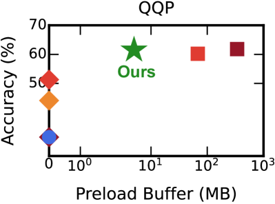
Compared to preloading the whole model, STI reduces memory consumption by 1-2 orders of magnitude while seeing 0.16 pp higher accuracy averaged across all latencies and benchmarks; compared to loading the model on demand, STI improves the accuracy by 14 pp at the cost of preload memory of no more than 5 MBs.

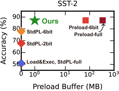
Figure 7 zooms in accuracy/memory tradeoffs under $T=200ms$ of SST and QQP benchmarks. Note that we use log scale in X-axis (memory consumption) due to its large span. STI uses 204$\times$ lower memory than PreloadModel-full while having less than 1% average accuracy loss. Even when compared with the quantized version (i.e. PreloadModel-6bit), STI uses on average 41$\times$ smaller memory to achieve the same accuracy.

Accuracy

STI’s accuracy matches those of DistilBERT. Given a target latency T, STI achieves consistent and significant accuracy gain over baselines. Table 5 shows the full view. On Odroid, STI (Ours) increases average accuracy by 21.05/21.05/17.13/5.83 pp compared with Load&Exec/StdPL-full/StdPL-2bit/StdPL-6bit, respectively. On Jetson, STI increases average accuracy by 18.77/18.77/6.53/3.15 pp compared with Load&Exec/StdPL-full/StdPL-2bit/StdPL-6bit, respectively. Notably, STI’s benefit is game-changing compared with Load&Exec and StdPL-full. They are barely usable under low latency (T$\leq$200ms).

Memory consumptions

Compared with preloading the whole model, STI reduces memory consumption significantly and consistently, by 122$\times$ on average. This is because the PrelodModel baselines hold the whole 12x12 model in memory. By comparison, STI only needs preload memory of 1MB/5MB on Odroid and Jetson respectively, which is sufficient to hold shards of the first model layer and warms up the pipeline execution.

Storage & energy overhead

For a model, STI only requires 215 MB disk space to store five fidelity versions of {2,3,4,5,6} bits, in addition to the full model (in 32 bits) of 418 MB. This storage overhead is minor given that today’s smartphone has tens or hundreds GB of storage.

For a given latency, we expect STI to consume notably more energy than low-accuracy baselines (e.g. Load&Exec, StdPL-full), as STI has higher resource utilization to achieve higher accuracy. Compared to similar-accuracy, high-memory baselines (i.e. PreloadModel-full), we expect STI to consume moderately but not significantly more energy. First, the major energy consumer is active compute (FLOPs); similar accuracies indicate similar FLOPs. Second, although STI adds IO activities, the contribution to the system power is marginal because the whole SoC is already in high power states.

(a) Odroid

(b) Jetson

Figure 7. STI’s accuracy is significantly higher than Load&Exec and StdPL, and is similar/higher compared to PreloadModel albeit using 1-2 orders of magnitude smaller memory. T=200ms. Full data and benchmarks in Table 5.

Table 6. Sizes (depth$\times$width) of submodels selected under different target latencies. A large submodel means more FLOPs executed, suggesting a higher accuracy. STI is able to run the largest submodel.

7.3. Significance of Key Designs

Submodel configuration

Within a given latency, the result accuracy hinges on total FLOPs executed, which depends on the size of executed submodel. Our results show that STI dynamically adjusts submodel sizes towards the maximum FLOPs. Table 6 shows the details. Estimated by comparing submodel sizes: our FLOPs is as high as that of PreloadModel, which however consumes 1-2 orders of magnitude more memory; our FLOPs is 7$\times$ higher compared with Load&Exec and StdPL-full, for which the IO blocks computation most of the time; our FLOPs is 1.3$\times$ higher than that of StdPL-2/6bit, two strong baselines that increase FLOPs through IO/compute parallelism and quantization as us; at lower T (e.g. $T\leq 200ms$), their IO delays of loading the first layer may block computation, resulting in a smaller model. Figure 8 shows such an example. Thanks to a small preload buffer, our executed submodel has 1.25$\times$ higher FLOPs (i.e. it has one extra layer), which leads to 9.2 percentage point (pp) higher accuracy.

Figure 8. A comparison between submodels executed by Ours and StdPL-6bit. Benchmark: SST-2 on Odroid. T=200ms. Ours runs a larger submodel and higher FLOPs, resulting in 9.2 pp higher accuracy.

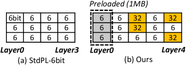
Table 6 also shows that our system adjusts submodels according to platform hardware. Specifically, our system assembles shallow/wide submodels on Jetson (GPU) as opposed to deeper/narrower submodels on Odroid (CPU). The reason is GPU’s lack of proportionality on Transformer shards, e.g. executing a layer of 12 shards is only 0.7% longer than a layer of 3 shards. The root cause is that GPU is optimized for batch workload; it pays a fixed, significant cost even in executing a fraction of a transformer layer and for one input example, which is the case of interactive NLP.

Elastic pipelining

STI’s per-shard bitwidths contribute to its accuracy significantly. By contrast, one fixed bitwidth for all shards in a model is too rigid, resulting in pipeline bubbles. With a full bitwidth of 32 bits (StdPL-full), IO takes long and stalls the computation (19.9 pp lower accuracy than STI); with a lower bitwidth (StdPL-{2,6}bit), IO bandwidth is left underutilized (8.2 pp lower accuracy than STI). Any fixed bitwidth between 6 and 32 bits does not help either (Section 7.1). Unlike them, STI well utilizes both compute and IO through its two-stage planning (§5).

Preload buffers

show a clear benefit as shown in Table 5. By using a small preload buffer of a few MBs, STI achieves a noticeable and consistent accuracy gain compared to not using the preload buffer (Ours-0MB). The benefit is most pronounced on QNLI and QQP among the benchmarks, increasing accuracy by up to 3.7 percent point (Odroid). Section 7.4 will present a sensitivity analysis regarding its size.

Shard importance

STI allocates its IO budgets to the most important shards. The accuracy benefit is most pronounced in a small/median submodel where most shards have low to medium bitwidths.

Case study. We demonstrate the efficacy through a differential analysis. Table 7 shows an intermediate state of planning: a 5x3 submodel comprising all 2-bit shards. Now the planner is awarded additional IO budgets, e.g. from enlargement of the preload buffer, with which the planner will increase some shards’ bitwidths to 6 bits. We compare two strategies: (1) randomly pick shards; (2) pick shards in their importance order (as in STI). Despite the same IO budget is spent, STI shows higher accuracy by up to 23.1 percent point (8.19 percent point on average) across all benchmarks.

Table 7. Model accuracies resultant from allocating additional IO budget within a 5x3 submodel of 2-bit shards. Our method shows much higher accuracies than random shard selection.

7.4. Sensitivity Analysis

We examine how STI’s benefit changes as resource amounts.

Target latencies

A more relaxed target latency allows STI to deliver more FLOPs and execute a deeper submodel, suggesting a higher accuracy. Yet, an NLP model’s accuracy sees diminishing return as its depth continues to grow, as shown in prior work (Fan et al., 2020; Hou et al., 2020); as a result, STI’s benefit diminishes as the target latency is further relaxed. Specifically, on Odroid (CPU) STI has most significant advantage over baselines (7.7 pp higher accuracy) when target latencies are below 200 ms; in such cases, a feasible submodel has fewer than 10 layers. On Jetson (GPU) STI has most significant advantage when target latencies are below 400 ms and a feasible submodel has fewer than 7 layers. When the target latency grows beyond such ranges, STI’s benefits gradually reduce.

Preload buffer size

Its significance hinges on the relative speeds of computation (which consumes model parameters) and IO (which loads the parameters), because the buffer bridges the speed gap of the two. When the computation is much faster than IO, an increase in the buffer size will result in large accuracy gain, and vice versa.

On our platforms, STI shows a noticeable and consistent accuracy gain over baselines by using a preload buffer of a few MBs. Since at current preload buffer size STI has already reached best accuracy (i.e. same as PreloadModel-full), further increasing the buffer size does not boost the accuracy proportionally. We expect that with faster compute (e.g. neural accelerators), the preload buffer takes in a greater role. The reason is, when execution become faster and can only overlap with loading of low-fidelity shards (e.g. 2 bits), a few high-fidelity shards provided by preload buffer can significantly boost the accuracy. Such a case is shown in Table 7, as preload buffer sizes increase from 0.4 to 4.0 MB, the accuracy increase by 19.2 pp.

8. Related work

Our system is related to a wide range of ML and systems techniques. We next discuss the similarities and differences.

Model compression

is a common technique for reducing model size (IO), facilitating faster loading; it includes model structure (Fan et al., 2020; Sanh et al., 2019) and feature pruning (Sun et al., 2020), and quantization which reduces full-precisions (32bit) parameters into low-bit (e.g. 2bit) representations (Qin et al., 2022; Bai et al., 2021; Zafrir et al., 2019; Han et al., 2016). We use quantization to compress the model; differently, we scale compression ratios to runtime IO by instantiating multiple compressed versions. Automated quantization searches for optimal bit-widths of a NN in the offline, often on a per layer basis (Wang et al., 2019; Dong et al., 2019; Liu et al., 2021). HAQ (Wang et al., 2019) adopts the reinforcement learning to find the best mixed precision for each layer, similar with our multiple versions of shards. Compared with them, we do not need any fine-tuning, which is time-consuming and we must make fine-grained decisions (i.e. per-shard) at run time.

Dynamic configuration of DNNs

changes model widths and/or depths in order to suit resource constraints (Hou et al., 2020; Tambe et al., 2021; Fan et al., 2020; Wang et al., 2020; Fang et al., 2018). EdgeBERT (Tambe et al., 2021) improves NLP energy efficiency under target latencies via early exit. NestDNN (Fang et al., 2018) hosts one multi-capacity model on device and switches across submodels depending on available resources. Assuming the whole model always held in memory, these systems miss the opportunities of pipelined IO/compute and therefore incur high memory cost when applied to NLP. Similar to them, we configure the NLP model architecture dynamically. Unlike them, we address the challenge of loading large models through pipelining. Furthermore, our configuration is on the basis of individual shards and adapts to both memory and latency constraints.

Pipeline parallelism for ML

Pipelining has been extensively used to accelerate ML. Prior work mainly uses it to scale out ML to multiple machines (overcome limit of single machine resource). Notably for training, PP is used to partition a model or training data over a cluster of machines (Huang et al., 2019) for maximizing hardware utilization by minimizing pipeline stalls using micro/minibatches (Narayanan et al., 2019), exploiting hardware heterogeneity (Hu et al., 2021), or by adapting pipeline depths on the fly (He et al., 2021). We share a similar goal of maximizing pipeline utilization and minimizing bubbles. Unlike that they focus on a pipeline of computations (forward/backward passes of different inputs) or network/computation, our pipeline consists of disk IO tasks and computation. Our approach towards high efficiency is through adjusting IO workloads of model shards to the computation.

9. Concluding remarks

We present STI, a novel system for speedy transformer inference on mobile devices. STI contributes two novel techniques: model sharding and elastic pipeline planning with a preload buffer. The former allows STI to tune model parameters at fine granularities in a resource-elastic fashion. The latter facilitates STI for maximizing IO/compute utilization on most important parts of the model. With them, STI reduces memory consumption by 1-2 orders of magnitude while delivering high accuracies under a practical range of target latencies.

References

- (1)
- ber (2022) 2022. Hugging Face:nlptown/bert-base-multilingual-uncased-sentiment. https://huggingface.co/nlptown/bert-base-multilingual-uncased-sentiment. (Accessed on 07/07/2022).
- pyt (2022) 2022. PyTorch. https://pytorch.org/. (Accessed on 03/14/2022).
- tor (2022) 2022. PyTorch 1.11, TorchData, and functorch are now available — PyTorch. https://pytorch.org/blog/pytorch-1.11-released/. (Accessed on 07/07/2022).
- ten (2022) 2022. TensorFlow. https://www.tensorflow.org/. (Accessed on 03/14/2022).
- skl (2022) 2022. Version 0.23.2 — scikit-learn 1.1.1 documentation. https://scikit-learn.org/stable/whats_new/v0.23.html. (Accessed on 07/07/2022).
- Android (2022) Android. 2022. Android: Low Memory Killer Daemon. https://source.android.com/devices/tech/perf/lmkd/.
- Bai et al. (2021) Haoli Bai, Wei Zhang, Lu Hou, Lifeng Shang, Jin Jin, Xin Jiang, Qun Liu, Michael R. Lyu, and Irwin King. 2021. BinaryBERT: Pushing the Limit of BERT Quantization. In Proceedings of the 59th Annual Meeting of the Association for Computational Linguistics and the 11th International Joint Conference on Natural Language Processing, ACL/IJCNLP 2021, (Volume 1: Long Papers), Virtual Event, August 1-6, 2021, Chengqing Zong, Fei Xia, Wenjie Li, and Roberto Navigli (Eds.). Association for Computational Linguistics, 4334–4348. https://doi.org/10.18653/v1/2021.acl-long.334
- Bhattacharjee et al. (2020) Kasturi Bhattacharjee, Miguel Ballesteros, Rishita Anubhai, Smaranda Muresan, Jie Ma, Faisal Ladhak, and Yaser Al-Onaizan. 2020. To BERT or Not to BERT: Comparing Task-specific and Task-agnostic Semi-Supervised Approaches for Sequence Tagging. In Proceedings of the 2020 Conference on Empirical Methods in Natural Language Processing, EMNLP 2020, Online, November 16-20, 2020, Bonnie Webber, Trevor Cohn, Yulan He, and Yang Liu (Eds.). Association for Computational Linguistics, 7927–7934. https://doi.org/10.18653/v1/2020.emnlp-main.636
- Bogers et al. (2019) Toine Bogers, Ammar Ali Abdelrahim Al-Basri, Claes Ostermann Rytlig, Mads Emil Bak Møller, Mette Juhl Rasmussen, Nikita Katrine Bates Michelsen, and Sara Gerling Jørgensen. 2019. A Study of Usage and Usability of Intelligent Personal Assistants in Denmark. In Information in Contemporary Society - 14th International Conference, iConference 2019, Washington, DC, USA, March 31 - April 3, 2019, Proceedings (Lecture Notes in Computer Science, Vol. 11420), Natalie Greene Taylor, Caitlin Christian-Lamb, Michelle H. Martin, and Bonnie A. Nardi (Eds.). Springer, 79–90. https://doi.org/10.1007/978-3-030-15742-5_7
- Carrascal and Church (2015) Juan Pablo Carrascal and Karen Church. 2015. An In-Situ Study of Mobile App & Mobile Search Interactions. In Proceedings of the 33rd Annual ACM Conference on Human Factors in Computing Systems, CHI 2015, Seoul, Republic of Korea, April 18-23, 2015, Bo Begole, Jinwoo Kim, Kori Inkpen, and Woontack Woo (Eds.). ACM, 2739–2748. https://doi.org/10.1145/2702123.2702486
- Cartas et al. (2019) Alejandro Cartas, Martin Kocour, Aravindh Raman, Ilias Leontiadis, Jordi Luque, Nishanth Sastry, José Núñez-Martínez, Diego Perino, and Carlos Segura. 2019. A Reality Check on Inference at Mobile Networks Edge. In Proceedings of the 2nd International Workshop on Edge Systems, Analytics and Networking, EdgeSys@EuroSys 2019, Dresden, Germany, March 25, 2019. ACM, 54–59. https://doi.org/10.1145/3301418.3313946
- Chen et al. (2019) Xiantao Chen, Moli Zhou, Renzhen Wang, Yalin Pan, Jiaqi Mi, Hui Tong, and Daisong Guan. 2019. Evaluating Response Delay of Multimodal Interface in Smart Device. In Design, User Experience, and Usability. Practice and Case Studies - 8th International Conference, DUXU 2019, Held as Part of the 21st HCI International Conference, HCII 2019, Orlando, FL, USA, July 26-31, 2019, Proceedings, Part IV (Lecture Notes in Computer Science, Vol. 11586), Aaron Marcus and Wentao Wang (Eds.). Springer, 408–419. https://doi.org/10.1007/978-3-030-23535-2_30
- Clark et al. (2019) Kevin Clark, Urvashi Khandelwal, Omer Levy, and Christopher D. Manning. 2019. What Does BERT Look at? An Analysis of BERT’s Attention. In Proceedings of the 2019 ACL Workshop BlackboxNLP: Analyzing and Interpreting Neural Networks for NLP, BlackboxNLP@ACL 2019, Florence, Italy, August 1, 2019, Tal Linzen, Grzegorz Chrupala, Yonatan Belinkov, and Dieuwke Hupkes (Eds.). Association for Computational Linguistics, 276–286. https://doi.org/10.18653/v1/W19-4828
- Dagum and Menon (1998) Leonardo Dagum and Ramesh Menon. 1998. OpenMP: an industry standard API for shared-memory programming. IEEE computational science and engineering 5, 1 (1998), 46–55.
- de Barcelos Silva et al. (2020) Allan de Barcelos Silva, Marcio Miguel Gomes, Cristiano André da Costa, Rodrigo da Rosa Righi, Jorge Luis Victoria Barbosa, Gustavo Pessin, Geert De Doncker, and Gustavo Federizzi. 2020. Intelligent Personal Assistants: A Systematic Literature Review. 147 (2020), 113193. https://doi.org/10.1016/j.eswa.2020.113193
- Devlin et al. (2019) Jacob Devlin, Ming-Wei Chang, Kenton Lee, and Kristina Toutanova. 2019. BERT: Pre-training of Deep Bidirectional Transformers for Language Understanding. In Proceedings of the 2019 Conference of the North American Chapter of the Association for Computational Linguistics: Human Language Technologies, NAACL-HLT 2019, Minneapolis, MN, USA, June 2-7, 2019, Volume 1 (Long and Short Papers), Jill Burstein, Christy Doran, and Thamar Solorio (Eds.). Association for Computational Linguistics, 4171–4186. https://doi.org/10.18653/v1/n19-1423
- Dong et al. (2019) Zhen Dong, Zhewei Yao, Amir Gholami, Michael W. Mahoney, and Kurt Keutzer. 2019. HAWQ: Hessian AWare Quantization of Neural Networks With Mixed-Precision. In 2019 IEEE/CVF International Conference on Computer Vision, ICCV 2019, Seoul, Korea (South), October 27 - November 2, 2019. IEEE, 293–302. https://doi.org/10.1109/ICCV.2019.00038
- Eisenman et al. (2019) Assaf Eisenman, Maxim Naumov, Darryl Gardner, Misha Smelyanskiy, Sergey Pupyrev, Kim M. Hazelwood, Asaf Cidon, and Sachin Katti. 2019. Bandana: Using Non-Volatile Memory for Storing Deep Learning Models. In Proceedings of Machine Learning and Systems 2019, MLSys 2019, Stanford, CA, USA, March 31 - April 2, 2019, Ameet Talwalkar, Virginia Smith, and Matei Zaharia (Eds.). mlsys.org. https://proceedings.mlsys.org/book/277.pdf
- Fan et al. (2020) Angela Fan, Edouard Grave, and Armand Joulin. 2020. Reducing Transformer Depth on Demand with Structured Dropout. In 8th International Conference on Learning Representations, ICLR 2020, Addis Ababa, Ethiopia, April 26-30, 2020. OpenReview.net. https://openreview.net/forum?id=SylO2yStDr
- Fang et al. (2018) Biyi Fang, Xiao Zeng, and Mi Zhang. 2018. NestDNN: Resource-Aware Multi-Tenant On-Device Deep Learning for Continuous Mobile Vision. In Proceedings of the 24th Annual International Conference on Mobile Computing and Networking, MobiCom 2018, New Delhi, India, October 29 - November 02, 2018, Rajeev Shorey, Rohan Murty, Yingying (Jennifer) Chen, and Kyle Jamieson (Eds.). ACM, 115–127. https://doi.org/10.1145/3241539.3241559
- Gong et al. (2019) ChengYue Gong, Zixuan Jiang, Dilin Wang, Yibo Lin, Qiang Liu, and David Z. Pan. 2019. Mixed Precision Neural Architecture Search for Energy Efficient Deep Learning. In Proceedings of the International Conference on Computer-Aided Design, ICCAD 2019, Westminster, CO, USA, November 4-7, 2019, David Z. Pan (Ed.). ACM, 1–7. https://doi.org/10.1109/ICCAD45719.2019.8942147
- Guo and Lin (2022) Liwei Guo and Felix Xiaozhu Lin. 2022. Minimum viable device drivers for ARM trustzone. In EuroSys ’22: Seventeenth European Conference on Computer Systems, Rennes, France, April 5 - 8, 2022, Yérom-David Bromberg, Anne-Marie Kermarrec, and Christos Kozyrakis (Eds.). ACM, 300–316. https://doi.org/10.1145/3492321.3519565
- Han et al. (2016) Song Han, Huizi Mao, and William J. Dally. 2016. Deep Compression: Compressing Deep Neural Network with Pruning, Trained Quantization and Huffman Coding. In 4th International Conference on Learning Representations, ICLR 2016, San Juan, Puerto Rico, May 2-4, 2016, Conference Track Proceedings, Yoshua Bengio and Yann LeCun (Eds.). http://arxiv.org/abs/1510.00149
- He et al. (2021) Chaoyang He, Shen Li, Mahdi Soltanolkotabi, and Salman Avestimehr. 2021. PipeTransformer: Automated Elastic Pipelining for Distributed Training of Large-scale Models. In Proceedings of the 38th International Conference on Machine Learning, ICML 2021, 18-24 July 2021, Virtual Event (Proceedings of Machine Learning Research, Vol. 139), Marina Meila and Tong Zhang (Eds.). PMLR, 4150–4159. http://proceedings.mlr.press/v139/he21a.html
- Hochreiter and Schmidhuber (1997) Sepp Hochreiter and Jürgen Schmidhuber. 1997. Long Short-Term Memory. Neural Computation 9, 8 (1997), 1735–1780. https://doi.org/10.1162/neco.1997.9.8.1735
- Hou et al. (2020) Lu Hou, Zhiqi Huang, Lifeng Shang, Xin Jiang, Xiao Chen, and Qun Liu. 2020. DynaBERT: Dynamic BERT with Adaptive Width and Depth. In Advances in Neural Information Processing Systems 33: Annual Conference on Neural Information Processing Systems 2020, NeurIPS 2020, December 6-12, 2020, virtual, Hugo Larochelle, Marc’Aurelio Ranzato, Raia Hadsell, Maria-Florina Balcan, and Hsuan-Tien Lin (Eds.). https://proceedings.neurips.cc/paper/2020/hash/6f5216f8d89b086c18298e043bfe48ed-Abstract.html
- Hu et al. (2021) Yang Hu, Connor Imes, Xuanang Zhao, Souvik Kundu, Peter A. Beerel, Stephen P. Crago, and John Paul Walters. 2021. Pipeline Parallelism for Inference on Heterogeneous Edge Computing. CoRR abs/2110.14895 (2021). arXiv:2110.14895 https://arxiv.org/abs/2110.14895
- Huang et al. (2019) Yanping Huang, Youlong Cheng, Ankur Bapna, Orhan Firat, Dehao Chen, Mia Xu Chen, HyoukJoong Lee, Jiquan Ngiam, Quoc V. Le, Yonghui Wu, and Zhifeng Chen. 2019. GPipe: Efficient Training of Giant Neural Networks using Pipeline Parallelism. In Advances in Neural Information Processing Systems 32: Annual Conference on Neural Information Processing Systems 2019, NeurIPS 2019, December 8-14, 2019, Vancouver, BC, Canada, Hanna M. Wallach, Hugo Larochelle, Alina Beygelzimer, Florence d’Alché-Buc, Emily B. Fox, and Roman Garnett (Eds.). 103–112. https://proceedings.neurips.cc/paper/2019/hash/093f65e080a295f8076b1c5722a46aa2-Abstract.html
- Lan et al. (2020) Zhenzhong Lan, Mingda Chen, Sebastian Goodman, Kevin Gimpel, Piyush Sharma, and Radu Soricut. 2020. ALBERT: A Lite BERT for Self-supervised Learning of Language Representations. In 8th International Conference on Learning Representations, ICLR 2020, Addis Ababa, Ethiopia, April 26-30, 2020. OpenReview.net. https://openreview.net/forum?id=H1eA7AEtvS
- Lebeck et al. (2020) Niel Lebeck, Arvind Krishnamurthy, Henry M. Levy, and Irene Zhang. 2020. End the Senseless Killing: Improving Memory Management for Mobile Operating Systems. In 2020 USENIX Annual Technical Conference, USENIX ATC 2020, July 15-17, 2020, Ada Gavrilovska and Erez Zadok (Eds.). USENIX Association, 873–887. https://www.usenix.org/conference/atc20/presentation/lebeck
- Lee and Bahn (2021) Soyoon Lee and Hyokyung Bahn. 2021. Characterization of Android Memory References and Implication to Hybrid Memory Management. IEEE Access 9 (2021), 60997–61009. https://doi.org/10.1109/ACCESS.2021.3074179
- Li et al. (2015) Huoran Li, Xuan Lu, Xuanzhe Liu, Tao Xie, Kaigui Bian, Felix Xiaozhu Lin, Qiaozhu Mei, and Feng Feng. 2015. Characterizing Smartphone Usage Patterns from Millions of Android Users. In Proceedings of the 2015 ACM Internet Measurement Conference, IMC 2015, Tokyo, Japan, October 28-30, 2015, Kenjiro Cho, Kensuke Fukuda, Vivek S. Pai, and Neil Spring (Eds.). ACM, 459–472. https://doi.org/10.1145/2815675.2815686
- Liu et al. (2019) Yinhan Liu, Myle Ott, Naman Goyal, Jingfei Du, Mandar Joshi, Danqi Chen, Omer Levy, Mike Lewis, Luke Zettlemoyer, and Veselin Stoyanov. 2019. RoBERTa: A Robustly Optimized BERT Pretraining Approach. CoRR abs/1907.11692 (2019). arXiv:1907.11692 http://arxiv.org/abs/1907.11692
- Liu et al. (2021) Zhenhua Liu, Xinfeng Zhang, Shanshe Wang, Siwei Ma, and Wen Gao. 2021. Evolutionary Quantization of Neural Networks with Mixed-Precision. In IEEE International Conference on Acoustics, Speech and Signal Processing, ICASSP 2021, Toronto, ON, Canada, June 6-11, 2021. IEEE, 2785–2789. https://doi.org/10.1109/ICASSP39728.2021.9413631
- Lorenser (2016) Thomas Lorenser. 2016. The DSP capabilities of arm cortex-m4 and cortex-m7 processors. ARM White Paper 29 (2016).
- McTear et al. (2016) Michael Frederick McTear, Zoraida Callejas, and David Griol. 2016. The conversational interface. Vol. 6. Springer.
- Miao and Lin (2021) Hongyu Miao and Felix Xiaozhu Lin. 2021. Enabling Large NNs on Tiny MCUs with Swapping. CoRR abs/2101.08744 (2021). arXiv:2101.08744 https://arxiv.org/abs/2101.08744
- Michel et al. (2019) Paul Michel, Omer Levy, and Graham Neubig. 2019. Are Sixteen Heads Really Better than One?. In Advances in Neural Information Processing Systems 32: Annual Conference on Neural Information Processing Systems 2019, NeurIPS 2019, December 8-14, 2019, Vancouver, BC, Canada, Hanna M. Wallach, Hugo Larochelle, Alina Beygelzimer, Florence d’Alché-Buc, Emily B. Fox, and Roman Garnett (Eds.). 14014–14024. https://proceedings.neurips.cc/paper/2019/hash/2c601ad9d2ff9bc8b282670cdd54f69f-Abstract.html
- Narayanan et al. (2019) Deepak Narayanan, Aaron Harlap, Amar Phanishayee, Vivek Seshadri, Nikhil R. Devanur, Gregory R. Ganger, Phillip B. Gibbons, and Matei Zaharia. 2019. PipeDream: generalized pipeline parallelism for DNN training. In Proceedings of the 27th ACM Symposium on Operating Systems Principles, SOSP 2019, Huntsville, ON, Canada, October 27-30, 2019, Tim Brecht and Carey Williamson (Eds.). ACM, 1–15. https://doi.org/10.1145/3341301.3359646
- Park and Lin (2021) Heejin Park and Felix Xiaozhu Lin. 2021. TinyStack: A Minimal GPU Stack for Client ML. CoRR abs/2105.05085 (2021). arXiv:2105.05085 https://arxiv.org/abs/2105.05085
- Pati et al. (2021) Suchita Pati, Shaizeen Aga, Nuwan Jayasena, and Matthew D. Sinclair. 2021. Demystifying BERT: Implications for Accelerator Design. CoRR abs/2104.08335 (2021). arXiv:2104.08335 https://arxiv.org/abs/2104.08335
- Qin et al. (2022) Haotong Qin, Yifu Ding, Mingyuan Zhang, Qinghua Yan, Aishan Liu, Qingqing Dang, Ziwei Liu, and Xianglong Liu. 2022. BiBERT: Accurate Fully Binarized BERT. In The Tenth International Conference on Learning Representations, ICLR 2022, Virtual Event, April 25-29, 2022. OpenReview.net. https://openreview.net/forum?id=5xEgrl_5FAJ
- Radford et al. (2019) Alec Radford, Jeffrey Wu, Rewon Child, David Luan, Dario Amodei, Ilya Sutskever, et al. 2019. Language models are unsupervised multitask learners. OpenAI blog 1, 8 (2019), 9.
- Sandler et al. (2018) Mark Sandler, Andrew G. Howard, Menglong Zhu, Andrey Zhmoginov, and Liang-Chieh Chen. 2018. MobileNetV2: Inverted Residuals and Linear Bottlenecks. In 2018 IEEE Conference on Computer Vision and Pattern Recognition, CVPR 2018, Salt Lake City, UT, USA, June 18-22, 2018. Computer Vision Foundation / IEEE Computer Society, 4510–4520. https://doi.org/10.1109/CVPR.2018.00474
- Sanh et al. (2019) Victor Sanh, Lysandre Debut, Julien Chaumond, and Thomas Wolf. 2019. DistilBERT, a distilled version of BERT: smaller, faster, cheaper and lighter. CoRR abs/1910.01108 (2019). arXiv:1910.01108 http://arxiv.org/abs/1910.01108
- Shepard et al. (2011) Clayton Shepard, Ahmad Rahmati, Chad Tossell, Lin Zhong, and Phillip Kortum. 2011. LiveLab: Measuring Wireless Networks and Smartphone Users in the Field. SIGMETRICS Perform. Eval. Rev. 38, 3 (Jan. 2011), 15–20. https://doi.org/10.1145/1925019.1925023
- Shi et al. (2021) Yangyang Shi, Yongqiang Wang, Chunyang Wu, Ching-Feng Yeh, Julian Chan, Frank Zhang, Duc Le, and Mike Seltzer. 2021. Emformer: Efficient memory transformer based acoustic model for low latency streaming speech recognition. In ICASSP 2021-2021 IEEE International Conference on Acoustics, Speech and Signal Processing (ICASSP). IEEE, 6783–6787.
- Sun et al. (2020) Zhiqing Sun, Hongkun Yu, Xiaodan Song, Renjie Liu, Yiming Yang, and Denny Zhou. 2020. MobileBERT: a Compact Task-Agnostic BERT for Resource-Limited Devices. In Proceedings of the 58th Annual Meeting of the Association for Computational Linguistics, ACL 2020, Online, July 5-10, 2020, Dan Jurafsky, Joyce Chai, Natalie Schluter, and Joel R. Tetreault (Eds.). Association for Computational Linguistics, 2158–2170. https://doi.org/10.18653/v1/2020.acl-main.195
- Tambe et al. (2021) Thierry Tambe, Coleman Hooper, Lillian Pentecost, Tianyu Jia, En-Yu Yang, Marco Donato, Victor Sanh, Paul N. Whatmough, Alexander M. Rush, David Brooks, and Gu-Yeon Wei. 2021. EdgeBERT: Sentence-Level Energy Optimizations for Latency-Aware Multi-Task NLP Inference. In MICRO ’21: 54th Annual IEEE/ACM International Symposium on Microarchitecture, Virtual Event, Greece, October 18-22, 2021. ACM, 830–844. https://doi.org/10.1145/3466752.3480095
- Tay et al. (2020) Yi Tay, Mostafa Dehghani, Dara Bahri, and Donald Metzler. 2020. Efficient Transformers: A Survey. CoRR abs/2009.06732 (2020). arXiv:2009.06732 https://arxiv.org/abs/2009.06732
- Tian et al. (2020) Yuan Tian, Ke Zhou, Mounia Lalmas, and Dan Pelleg. 2020. Identifying Tasks from Mobile App Usage Patterns. In Proceedings of the 43rd International ACM SIGIR conference on research and development in Information Retrieval, SIGIR 2020, Virtual Event, China, July 25-30, 2020, Jimmy Huang, Yi Chang, Xueqi Cheng, Jaap Kamps, Vanessa Murdock, Ji-Rong Wen, and Yiqun Liu (Eds.). ACM, 2357–2366. https://doi.org/10.1145/3397271.3401441
- Vaswani et al. (2017) Ashish Vaswani, Noam Shazeer, Niki Parmar, Jakob Uszkoreit, Llion Jones, Aidan N. Gomez, Lukasz Kaiser, and Illia Polosukhin. 2017. Attention is All you Need. In Advances in Neural Information Processing Systems 30: Annual Conference on Neural Information Processing Systems 2017, December 4-9, 2017, Long Beach, CA, USA, Isabelle Guyon, Ulrike von Luxburg, Samy Bengio, Hanna M. Wallach, Rob Fergus, S. V. N. Vishwanathan, and Roman Garnett (Eds.). 5998–6008. https://proceedings.neurips.cc/paper/2017/hash/3f5ee243547dee91fbd053c1c4a845aa-Abstract.html
- Voita et al. (2019) Elena Voita, David Talbot, Fedor Moiseev, Rico Sennrich, and Ivan Titov. 2019. Analyzing Multi-Head Self-Attention: Specialized Heads Do the Heavy Lifting, the Rest Can Be Pruned. In Proceedings of the 57th Conference of the Association for Computational Linguistics, ACL 2019, Florence, Italy, July 28- August 2, 2019, Volume 1: Long Papers, Anna Korhonen, David R. Traum, and Lluís Màrquez (Eds.). Association for Computational Linguistics, 5797–5808. https://doi.org/10.18653/v1/p19-1580
- Wan et al. (2021) Hu Wan, Xuan Sun, Yufei Cui, Chia-Lin Yang, Tei-Wei Kuo, and Chun Jason Xue. 2021. FlashEmbedding: storing embedding tables in SSD for large-scale recommender systems. In APSys ’21: 12th ACM SIGOPS Asia-Pacific Workshop on Systems, Hong Kong, China, August 24-25, 2021, Haryadi S. Gunawi and Xiaosong Ma (Eds.). ACM, 9–16. https://doi.org/10.1145/3476886.3477511
- Wang et al. (2018) Alex Wang, Amanpreet Singh, Julian Michael, Felix Hill, Omer Levy, and Samuel R. Bowman. 2018. GLUE: A Multi-Task Benchmark and Analysis Platform for Natural Language Understanding. In Proceedings of the Workshop: Analyzing and Interpreting Neural Networks for NLP, BlackboxNLP@EMNLP 2018, Brussels, Belgium, November 1, 2018, Tal Linzen, Grzegorz Chrupala, and Afra Alishahi (Eds.). Association for Computational Linguistics, 353–355. https://doi.org/10.18653/v1/w18-5446
- Wang (2020) Hanrui Wang. 2020. Efficient Algorithms and Hardware for Natural Language Processing. PhD dissertation. Massachusetts Institute of Technology.
- Wang et al. (2020) Hanrui Wang, Zhanghao Wu, Zhijian Liu, Han Cai, Ligeng Zhu, Chuang Gan, and Song Han. 2020. HAT: Hardware-Aware Transformers for Efficient Natural Language Processing. In Proceedings of the 58th Annual Meeting of the Association for Computational Linguistics, ACL 2020, Online, July 5-10, 2020, Dan Jurafsky, Joyce Chai, Natalie Schluter, and Joel R. Tetreault (Eds.). Association for Computational Linguistics, 7675–7688. https://doi.org/10.18653/v1/2020.acl-main.686
- Wang et al. (2019) Kuan Wang, Zhijian Liu, Yujun Lin, Ji Lin, and Song Han. 2019. HAQ: Hardware-Aware Automated Quantization With Mixed Precision. In IEEE Conference on Computer Vision and Pattern Recognition, CVPR 2019, Long Beach, CA, USA, June 16-20, 2019. Computer Vision Foundation / IEEE, 8612–8620. https://doi.org/10.1109/CVPR.2019.00881
- Wang et al. (2021) Manni Wang, Shaohua Ding, Ting Cao, Yunxin Liu, and Fengyuan Xu. 2021. AsyMo: scalable and efficient deep-learning inference on asymmetric mobile CPUs. In ACM MobiCom ’21: The 27th Annual International Conference on Mobile Computing and Networking, New Orleans, Louisiana, USA, October 25-29, 2021. ACM, 215–228. https://doi.org/10.1145/3447993.3448625
- Wilkening et al. (2021) Mark Wilkening, Udit Gupta, Samuel Hsia, Caroline Trippel, Carole-Jean Wu, David Brooks, and Gu-Yeon Wei. 2021. RecSSD: Near Data Processing for Solid State Drive Based Recommendation Inference. In Proceedings of the 26th ACM International Conference on Architectural Support for Programming Languages and Operating Systems (Virtual USA, 2021-04-19). ACM, 717–729. https://doi.org/10.1145/3445814.3446763
- Yang et al. (2020) Luting Yang, Bingqian Lu, and Shaolei Ren. 2020. A Note on Latency Variability of Deep Neural Networks for Mobile Inference. CoRR abs/2003.00138 (2020). arXiv:2003.00138 https://arxiv.org/abs/2003.00138
- Yi et al. (2022) Rongjie Yi, Ting Cao, Ao Zhou, Xiao Ma, Shangguang Wang, and Mengwei Xu. 2022. Understanding and Optimizing Deep Learning Cold-Start Latency on Edge Devices. https://doi.org/10.48550/ARXIV.2206.07446
- Yu et al. (2020) Haonan Yu, Sergey Edunov, Yuandong Tian, and Ari S. Morcos. 2020. Playing the lottery with rewards and multiple languages: lottery tickets in RL and NLP. In 8th International Conference on Learning Representations, ICLR 2020, Addis Ababa, Ethiopia, April 26-30, 2020. OpenReview.net. https://openreview.net/forum?id=S1xnXRVFwH
- Zadeh et al. (2020) Ali Hadi Zadeh, Isak Edo, Omar Mohamed Awad, and Andreas Moshovos. 2020. GOBO: Quantizing Attention-Based NLP Models for Low Latency and Energy Efficient Inference. In 2020 53rd Annual IEEE/ACM International Symposium on Microarchitecture (MICRO) (Athens, Greece, 2020-10). IEEE, 811–824. https://doi.org/10.1109/MICRO50266.2020.00071
- Zafrir et al. (2019) Ofir Zafrir, Guy Boudoukh, Peter Izsak, and Moshe Wasserblat. 2019. Q8BERT: Quantized 8Bit BERT. In Fifth Workshop on Energy Efficient Machine Learning and Cognitive Computing - NeurIPS Edition, EMC2@NeurIPS 2019, Vancouver, Canada, December 13, 2019. IEEE, 36–39. https://doi.org/10.1109/EMC2-NIPS53020.2019.00016
- Zhang et al. (2018) Xiangyu Zhang, Xinyu Zhou, Mengxiao Lin, and Jian Sun. 2018. ShuffleNet: An Extremely Efficient Convolutional Neural Network for Mobile Devices. In 2018 IEEE Conference on Computer Vision and Pattern Recognition, CVPR 2018, Salt Lake City, UT, USA, June 18-22, 2018. Computer Vision Foundation / IEEE Computer Society, 6848–6856. https://doi.org/10.1109/CVPR.2018.00716