MIMO Symbiotic Radio with Massive
Passive Devices: Asymptotic Analysis
and Precoding Optimization

Jingran Xu, Zhuoyin Dai, and Yong Zeng This work was supported by the National Key R&D Program of China with grant number 2019YFB1803400, by the Natural Science Foundation of China under Grant 62071114, and also by the Fundamental Research Funds for the Central Universities 2242022k30005. Part of this work has been presented at the 2021 IEEE GLOBECOM, Madrid, Spain, 7-11 Dec. 2021 [7].The authors are with the National Mobile Communications Research Laboratory and Frontiers Science Center for Mobile Information Communication and Security, Southeast University, Nanjing 210096, China. Y. Zeng is also with the Purple Mountain Laboratories, Nanjing 211111, China (e-mail: jingranxu, zhuoyindai, yongzeng@seu.edu.cn). (Corresponding author: Yong Zeng.)
Abstract

Symbiotic radio has emerged as a promising technology for spectrum- and energy-efficient wireless communications, where the passive secondary backscatter devices (BDs) reuse not only the spectrum but also the power of the active primary users to transmit their own information. In return, the primary communication links can be enhanced by the additional multipaths created by the BDs. This is known as the mutualism relationship of symbiotic radio. However, due to the severe double-fading attenuation of the passive backscattering links, the enhancement of the primary link provided by one single BD is extremely limited. To address this issue and enable full mutualism of symbiotic radio, in this paper, we study multiple-input multiple-output (MIMO) symbiotic radio communication systems with massive BDs. We first derive the achievable rates of the primary active communication and secondary passive communication, and then consider the asymptotic regime as the number of BDs goes large, for which closed-form expressions are derived to reveal the relationship between the primary and secondary communication rates. Furthermore, the precoding optimization problem is studied to maximize the primary communication rate while guaranteeing that the secondary communication rate is no smaller than a certain threshold. Simulation results are provided to validate our theoretical studies.

Index Terms:
MIMO symbiotic radio, backscattering, massive passive devices, active and passive communication, asymptotic analysis

I Introduction

Symbiotic radio has emerged as a new paradigm to achieve both spectrum-efficient and energy-efficient wireless communications, for which the secondary user modulates its information over the radio frequency (RF) signals received from primary transmitter (PT) [1, 2, 3]. As such, the secondary backscatter device (BD) in symbiotic radio systems leverages not only the spectrum as in the extensively studied cognitive radio systems [4, 5, 6], but also the energy of the primary signals via passive backscattering technology for its own information transmission. To overcome the shortcoming of poor reliability suffered from the conventional passive ambient backscatter communication (AmBC) receiver [8, 9, 10], symbiotic radio introduces cooperation between the backscatter transmission and the primary transmission by using a joint receiver. Depending on the relations between the symbol durations of the primary and secondary signals, symbiotic radio can be classified into parasite symbiotic radio (PSR) and commensal symbiotic radio (CSR) [11]. In PSR, the secondary and primary signals have equal symbol durations, so that the information transmission of BD interferes with the primary transmission. By contrast, for CSR, the symbol duration of BD signals is much longer than that of the primary signals, so that the backscattering signal of the BD may create additional multipaths to enhance the primary communication links. This is known as the mutualism relationship of symbiotic radio [11]. The mutualism spectrum sharing and low power consumption nature of symbiotic radio render it an attractive massive access technology for the sixth-generation (6G) mobile communication networks [12, 13, 14], to realize spectrum- and energy-efficient Internet of Things (IoT). By riding over different types of primary networks, there are many emerging applications for symbiotic radio, such as e-health, smart home, and environmental monitoring [1].

Significant research efforts have been recently devoted to the theoretical analysis and performance optimization of symbiotic radio systems. For example, the performance analysis in terms of achievable rate [15, 16], channel capacity [17] and outage probability [18] are given in different setups. By exploiting multi-antenna techniques for performance enhancement, multiple-input-single-output (MISO) and multiple-input-multiple-output (MIMO) symbiotic radio systems are investigated in [15, 19, 20]. Furthermore, beamforming optimization problems have been studied to maximize various performance metrics, such as energy efficiency [15], sum capacity of the primary and secondary communications [19], and fairness of the secondary users [20]. Besides, energy efficiency (EE) studies for symbiotic radio systems have also received growing attentions recently [21, 22, 23]. For example, in [21] and [22], the EE of symbiotic radio is defined as the ratio of the total throughput of all links to the total energy consumption of the network, while [23] characterizes the EE region of symbiotic radio systems, which is defined as all the achievable EE pairs by the active PT and passive BD. In addition, the combination of symbiotic radio with other technologies has also been investigated. For example, systems integrating non-orthogonal-multiple-access (NOMA) into symbiotic radio have been studied in [18, 24, 25]. In [26, 27], full-duplex technique is introduced into a symbiotic radio system, which enables a BD to transmit and receive information simultaneously. In [28], cell-free networking architecture is integrated with symbiotic radio transmission technology to realize passive communication with high macro-diversity.

Note that due to the severe double-fading attenuation, the strength of the backscattering link is usually much weaker than that of the direct link, which results in low data rates for the secondary communication and only marginal enhancement to the primary transmission by the backscattering link in the CSR setup. To address such issues, various techniques have been proposed, such as the active-load assisted [29, 30, 31] symbiotic radio by using negative resistances, or reconfigurable intelligent surface (RIS) aided [32, 33, 34] symbiotic radio by configuring large scale passive reflecting elements. However, the use of active loads requires additional power supply to generate the negative resistances, and a large scale deployment in RIS may not be suitable for many IoT devices that have small form factors. Thus, such existing techniques for enhancing the secondary communication links may increase the cost and complexity of the passive BD, which undermines the initial motivation of symbiotic radio.

In this paper, we propose an alternative method to significantly enhance the secondary backscattering links and enable the full mutualism of symbiotic radio systems, by exploiting the potential gain brought by multiple BDs, which provides abundant multi-user diversities for secondary communications and multipath gains for primary transmission. This is motivated by the 6G visions to support ultra-massive connectivity, say 10 million devices per square kilometer [35], most of which are expected to be IoT devices. Our main contributions are summarized as follows:

  • First, we present the mathematical model of MIMO symbiotic radio communication systems with multiple BDs in the CSR setup, where the mutualism relationship of symbiotic radio can be fully exploited. We derive the achievable rate expression of the primary communication, as well as the sum rate expression of the passive BDs, by noting that it corresponds to a multiple access channel (MAC) where minimum mean square error estimation (MMSE) with successive interference cancellation (SIC) is optimal [36].

  • Next, to show how the achievable communication rates of symbiotic radio are affected by the number of BDs, we consider the asymptotic analysis as the number of BDs goes large. Closed-form expressions are derived for the primary active communication rate and secondary passive communication rate, both of which are shown to be increasing functions of the number of BDs. For the special case of single-input-multiple-output (SIMO) symbiotic radio setup, we derive the closed-form expression of the asymptotic primary communication rate as a function of the asymptotic secondary sum-rate, which is revealed to be an increasing function. This thus demonstrates that the mutualism relationship of symbiotic radio can be fully enabled with massive BD access.

  • Furthermore, we formulate a precoding optimization problem to maximize the primary communication rate by taking into account the additional multipaths created by the BDs, while guaranteeing that the secondary communication rate is no smaller than a certain threshold. The problem is non-convex in its original form, and we propose an effective technique to transform it to an equivalent convex problem of optimizing the transmit covariance matrix. Two solutions with different trade-offs between complexity and performance are proposed, namely sample-average based solution and upper bound based solution. Numerical results are provided to demonstrate that the proposed optimization approaches are effective in MIMO symbiotic radio communication systems.

The rest of this paper is organized as follows. Section II presents the system model of MIMO symbiotic radio communication with multiple BDs. Section III derives the achievable rate of the primary communication and the sum rate of the secondary BDs. In Section IV, by assuming that the number of BDs goes large, asymptotic performance analysis is provided to reveal the relationship between primary active communication and secondary passive communication. In Section V, the precoding optimization problem is studied to maximize the primary communication rate while guaranteeing that the secondary communication rate is no smaller than a certain threshold. Section VI presents numerical results to validate our theoretical studies. Finally, we conclude the paper in Section VII.

Notations: In this paper, scalars are denoted by italic letters. Vectors and matrices are denoted by boldface lower-and upper-case letters, respectively. For a vector 𝐚𝐚\mathbf{a}, its transpose, Hermitian transpose, and Euclidean norm are respectively denoted as 𝐚Tsuperscript𝐚T\mathbf{a}^{\text{T}}, 𝐚Hsuperscript𝐚H\mathbf{a}^{\text{H}} and 𝐚norm𝐚\|\mathbf{a}\|. The conjugate, transpose, Hermitian transpose and rank of a matrix 𝐀𝐀\mathbf{A} are denoted as 𝐀superscript𝐀{{\mathbf{A}}^{*}}, 𝐀Tsuperscript𝐀T{{\mathbf{A}}^{\text{T}}}, 𝐀Hsuperscript𝐀H{{\mathbf{A}}^{\text{H}}} and rank(𝐀)rank𝐀\text{rank}(\mathbf{A}), respectively. vec(𝐀)vec𝐀\text{vec}(\mathbf{A}) represents stacking the columns of matrix 𝐀𝐀\mathbf{A} into a column vector. For a square matrix 𝐁𝐁\mathbf{B}, tr(𝐁)tr𝐁{\rm tr}(\mathbf{B}), |𝐁|𝐁\left|\mathbf{B}\right|, 𝐁1superscript𝐁1{{\mathbf{B}}^{-1}}, and 𝐁12superscript𝐁12{{\mathbf{B}}^{\frac{1}{2}}} denote its trace, determinant, inverse, and matrix square-root, respectively, while 𝐁0succeeds-or-equals𝐁0\mathbf{B}\succeq 0 represents that the matrix 𝐁𝐁\mathbf{B} is positive semidefinite. λ_1(𝐁),,λ_M(𝐁)subscript𝜆_1𝐁subscript𝜆_𝑀𝐁{{\lambda}_{\_}{1}(\mathbf{B})},...,{{\lambda}_{\_}{M}(\mathbf{B})} denote the eigenvalues of 𝐁𝐁\mathbf{B}. tensor-product\otimes refers to the Kronecker product. diag(x_1,,x_M)subscript𝑥_1subscript𝑥_𝑀(x_{\_}1,...,x_{\_}M) denotes an M×M𝑀𝑀M\times M diagonal matrix with x_1,,x_Msubscript𝑥_1subscript𝑥_𝑀x_{\_}1,...,x_{\_}M being the diagonal elements. 𝐈_Msubscript𝐈_𝑀\mathbf{I}_{\_}M denotes an M×M𝑀𝑀M\times M identity matrix. M×Nsuperscript𝑀𝑁\mathbb{C}^{M\times N} denotes the space of M×N𝑀𝑁{M\times N} matrices with complex entries. 𝔼_X[]subscript𝔼_𝑋delimited-[]\mathbb{E}_{\_}{X}[\cdot] denotes the expectation with respect to the random variable X𝑋X. log_2()subscript_2\log_{\_}{2}(\cdot) denotes the logarithm with base 2. Furthermore, 𝒞𝒩(𝐱,𝚺)𝒞𝒩𝐱𝚺\mathcal{CN}(\mathbf{x},\mathbf{\Sigma}) denotes the distribution of a circularly symmetric complex Gaussian (CSCG) random vector with mean 𝐱𝐱\mathbf{x} and covariance matrix 𝚺𝚺\mathbf{\Sigma}.

II System Model

Refer to caption

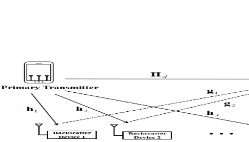
Figure 1: MIMO symbiotic radio with massive backscatter devices.

As shown in Fig. 1, we consider a MIMO symbiotic radio communication system, which consists of one PT, one access point (AP) and J𝐽J BDs. We assume that the PT and AP have M_tsubscript𝑀_𝑡M_{\_}t and M_rsubscript𝑀_𝑟M_{\_}r antennas, respectively, and each BD is equipped with one antenna. The AP wishes to decode not only the primary information from the PT, but also the secondary information from the J𝐽J BDs, which modulate their information via passively backscattering the incident signal from the PT. As such, the BDs reuse not only the spectrum but also the power of the PT. In return, their scattered signals may create additional channel paths to enhance the primary communication link, as long as their symbol rate is much lower than that of the primary signal. This is known as mutualism relationship of symbiotic radio[11]. Denote the MIMO direct-link channel from the PT to the AP as 𝐇_dM_r×M_tsubscript𝐇_𝑑superscriptsubscript𝑀_𝑟subscript𝑀_𝑡{{\mathbf{H}}_{\_}{d}}\in{{\mathbb{C}}^{M_{\_}r\times M_{\_}t}}. Further denote by 𝐡_jM_t×1subscript𝐡_𝑗superscriptsubscript𝑀_𝑡1{\mathbf{h}_{\_}{j}}\in\mathbb{C}^{M_{\_}t\times 1} the MISO channel from the PT to BD j𝑗j, and 𝐠_jM_r×1subscript𝐠_𝑗superscriptsubscript𝑀_𝑟1\mathbf{g}_{\_}j\in\mathbb{C}^{M_{\_}r\times 1} the SIMO channel from BD j𝑗j to the AP, where j=1,,J𝑗1𝐽j=1,...,J. Then the channel matrix for the cascaded backscattering link from the PT to AP via BD j𝑗j is 𝐠_j𝐡_jHsubscript𝐠_𝑗subscript𝐡_superscript𝑗H\mathbf{g}_{\_}j\mathbf{h}_{\_}{j}^{\text{H}}.

We focus on the CSR setup [11], where the symbol duration of the BDs is K1much-greater-than𝐾1K\gg 1 times of that of the PT. Let c_j(n)subscript𝑐_𝑗𝑛c_{\_}j(n) denote the independent and identically distributed (i.i.d.) information-bearing symbols of BD j𝑗j, and 𝐬(k,n)M_s×1𝐬𝑘𝑛superscriptsubscript𝑀_𝑠1\mathbf{s}(k,n)\in\mathbb{C}^{M_{\_}s\times 1} denote the i.i.d. information-bearing symbols of the PT, which follows CSCG distribution with normalized power, i.e., 𝐬(k,n)𝒞𝒩(𝟎,𝐈_M_s)similar-to𝐬𝑘𝑛𝒞𝒩0subscript𝐈_subscript𝑀_𝑠\mathbf{s}(k,n)\sim\mathcal{C}\mathcal{N}(\boldsymbol{0},\mathbf{I}_{\_}{M_{\_}s}), k=1,,K𝑘1𝐾k=1,...,K. Note that M_sM_tsubscript𝑀_𝑠subscript𝑀_𝑡M_{\_}s\leq M_{\_}t denotes the number of data streams of the PT signal, which is one of the optimization variables to be determined later. Furthermore, let P𝑃P denote the transmit power by the PT, α[0,1]𝛼01\alpha\in\left[0,1\right] be the fraction of the power backscattered by each BD, and 𝐅M_t×M_s𝐅superscriptsubscript𝑀_𝑡subscript𝑀_𝑠\mathbf{F}\in{{\mathbb{C}}^{M_{\_}t\times M_{\_}s}} denote the transmit precoding matrix of the PT, with tr(𝐅𝐅H)=1trsuperscript𝐅𝐅H1\text{tr}(\mathbf{F}{{\mathbf{F}}^{\text{H}}})=1. Then the signal received by the AP during the n𝑛nth BD symbol duration is

𝐲(k,n)=P𝐇_d𝐅𝐬(k,n)+_j=1JPα𝐠_j𝐡_jH𝐅𝐬(k,n)c_j(n)𝐲𝑘𝑛𝑃subscript𝐇_𝑑𝐅𝐬𝑘𝑛subscript_𝑗superscript1𝐽𝑃𝛼subscript𝐠_𝑗subscript𝐡_superscript𝑗H𝐅𝐬𝑘𝑛subscript𝑐_𝑗𝑛\displaystyle\mathbf{y}(k,n)=\sqrt{P}{{\mathbf{H}}_{\_}{d}}\mathbf{Fs}(k,n)+\sum\limits_{\_}{j=1}^{J}{\sqrt{P}}\sqrt{\alpha}{{\mathbf{g}}_{\_}{j}}{{\mathbf{h}}_{\_}{j}^{\text{H}}}\mathbf{Fs}(k,n){{c}_{\_}{j}}(n) (1)
+𝐳(k,n),k=1,,K,formulae-sequence𝐳𝑘𝑛𝑘1𝐾\displaystyle+\mathbf{z}(k,n),k=1,...,K,

where 𝐳(k,n)M_r×1𝐳𝑘𝑛superscriptsubscript𝑀_𝑟1\mathbf{z}(k,n)\in\mathbb{C}^{M_{\_}r\times 1} is the i.i.d. CSCG noise with zero mean and power σ2superscript𝜎2{{\sigma}^{2}}, i.e., 𝐳(k,n)𝒞𝒩(𝟎,σ2𝐈_M_r)similar-to𝐳𝑘𝑛𝒞𝒩0superscript𝜎2subscript𝐈_subscript𝑀_𝑟\mathbf{z}(k,n)\sim\mathcal{C}\mathcal{N}\left(\mathbf{0},\sigma^{2}{\mathbf{I}}_{\_}{M_{\_}r}\right).

III Achievable Rate Analysis

Since the BD symbols c_j(n)subscript𝑐_𝑗𝑛c_{\_}j(n) remain unchanged for each block of K𝐾K PT symbols, the second term in (1) constitutes additional multi-path channel components for the primary signal. As a result, the equivalent MIMO channel for decoding 𝐬(k,n)M_s×1𝐬𝑘𝑛superscriptsubscript𝑀_𝑠1\mathbf{s}(k,n)\in\mathbb{C}^{M_{\_}s\times 1} is dependent on the BD symbols 𝐜(n)=[c_1(n),c_2(n),,c_J(n)]T𝐜𝑛superscriptsubscript𝑐_1𝑛subscript𝑐_2𝑛subscript𝑐_𝐽𝑛T\mathbf{c}(n)=[c_{\_}1(n),c_{\_}2(n),...,c_{\_}J(n)]^{\text{T}}, which is denoted as 𝐇_eq(𝐜(n))=𝐇_d+_j=1Jα𝐠_j𝐡_jHc_j(n)subscript𝐇_𝑒𝑞𝐜𝑛subscript𝐇_𝑑subscript_𝑗superscript1𝐽𝛼subscript𝐠_𝑗subscript𝐡_superscript𝑗Hsubscript𝑐_𝑗𝑛{{\mathbf{H}}_{\_}{eq}}(\mathbf{c}(n))={{\mathbf{H}}_{\_}{d}}+\sum\limits_{\_}{j=1}^{J}{\sqrt{\alpha}}{{\mathbf{g}}_{\_}{j}}\mathbf{h}_{\_}{j}^{\text{H}}{{c}_{\_}{j}}(n). Therefore, (1) can also be expressed as

𝐲(k,n)=P𝐇_eq(𝐜(n))𝐅𝐬(k,n)+𝐳(k,n),k=1,,K.formulae-sequence𝐲𝑘𝑛𝑃subscript𝐇_𝑒𝑞𝐜𝑛𝐅𝐬𝑘𝑛𝐳𝑘𝑛𝑘1𝐾{\mathbf{y}(k,n)=\sqrt{P}{{\mathbf{H}}_{\_}{eq}}(\mathbf{c}(n))\mathbf{Fs}(k,n)+\mathbf{z}(k,n)},k=1,...,K. (2)

Note that (2) is essentially a block fading channel where the MIMO channel matrix 𝐇_eq(𝐜(n))subscript𝐇_𝑒𝑞𝐜𝑛{\mathbf{H}_{\_}{eq}(\mathbf{c}(n))} remains unchanged in each block n𝑛n of K𝐾K symbol durations, while varies across different blocks according to the BD symbols 𝐜(n)𝐜𝑛\mathbf{c}(n). We assume that the AP has the knowledge of the equivalent MIMO channel 𝐇_eq(𝐜(n))subscript𝐇_𝑒𝑞𝐜𝑛{\mathbf{H}}_{\_}{eq}(\mathbf{c}(n)), e.g., via standard training-based MIMO channel estimation [37], while the PT only knows the information of 𝐇_dsubscript𝐇_𝑑{\mathbf{H}}_{\_}{d}, 𝐡_jsubscript𝐡_𝑗\mathbf{h}_{\_}{j} and 𝐠_jsubscript𝐠_𝑗\mathbf{g}_{\_}j, but not 𝐇_eq(𝐜(n))subscript𝐇_𝑒𝑞𝐜𝑛{\mathbf{H}}_{\_}{eq}(\mathbf{c}(n)), since the BD symbols 𝐜(n)𝐜𝑛\mathbf{c}(n) are unknown at the PT. In this case, with a sufficiently large K𝐾K, the average primary communication rate for the input-output relationship (2) is

R_s=𝔼_𝐜(n)[log_2|𝐈_M_r+P¯𝐇_eq(𝐜(n))𝐅𝐅H𝐇_eqH(𝐜(n))|],subscript𝑅_𝑠subscript𝔼_𝐜𝑛delimited-[]subscript_2subscript𝐈_subscript𝑀_𝑟¯𝑃subscript𝐇_𝑒𝑞𝐜𝑛superscript𝐅𝐅Hsubscript𝐇_𝑒superscript𝑞H𝐜𝑛\begin{split}{{R}_{\_}{s}}={{\mathbb{E}}_{\_}{\mathbf{c}(n)}}\left[{{\log}_{\_}{2}}\left|{{\mathbf{I}}_{\_}{M_{\_}r}}+{\bar{P}}{{\mathbf{H}}_{\_}{eq}}\left(\mathbf{c}\left(n\right)\right)\mathbf{F}{{\mathbf{F}}^{\text{H}}}\mathbf{H}_{\_}{eq}^{\text{H}}\left(\mathbf{c}\left(n\right)\right)\right|\right],\end{split} (3)

where P¯Pσ2¯𝑃𝑃superscript𝜎2{\bar{P}}\triangleq\frac{P}{{{\sigma}^{2}}} is defined as the transmit signal-to-noise ratio (SNR).

On the other hand, to decode the symbols c_j(n)subscript𝑐_𝑗𝑛c_{\_}j(n) for each BD j𝑗j, by concatenating 𝐲(k,n)𝐲𝑘𝑛\mathbf{y}(k,n) in (1) for all k=1,2,,K𝑘12𝐾k=1,2,\cdots,K, we have 𝐘(n)=[𝐲(1,n),𝐲(2,n),,𝐲(K,n)]M_r×K𝐘𝑛𝐲1𝑛𝐲2𝑛𝐲𝐾𝑛superscriptsubscript𝑀_𝑟𝐾\mathbf{Y}(n)=\left[\mathbf{y}(1,n),\mathbf{y}(2,n),\cdots,\mathbf{y}(K,n)\right]\in\mathbb{C}^{M_{\_}r\times K}. Similarly, let 𝐒(n)=[𝐬(1,n),𝐬(2,n),,𝐬(K,n)]M_s×K𝐒𝑛𝐬1𝑛𝐬2𝑛𝐬𝐾𝑛superscriptsubscript𝑀_𝑠𝐾\mathbf{S}(n)={\left[{\mathbf{s}}{(1,n)},{\mathbf{s}}{(2,n)},\cdots,{\mathbf{s}}{(K,n)}\right]\in\mathbb{C}^{M_{\_}s\times K}} and 𝐙(n)=[𝐳(1,n),𝐳(2,n),,𝐳(K,n)]M_r×K𝐙𝑛𝐳1𝑛𝐳2𝑛𝐳𝐾𝑛superscriptsubscript𝑀_𝑟𝐾\mathbf{Z}(n)=\left[\mathbf{z}(1,n),\mathbf{z}(2,n),\cdots,\mathbf{z}(K,n)\right]\in\mathbb{C}^{M_{\_}r\times K}. Then (1) can be compactly written as

𝐘(n)=P𝐇_d𝐅𝐒(n)+_j=1JPα𝐠_j𝐡_jH𝐅𝐒(n)c_j(n)+𝐙(n).𝐘𝑛𝑃subscript𝐇_𝑑𝐅𝐒𝑛subscript_𝑗superscript1𝐽𝑃𝛼subscript𝐠_𝑗subscript𝐡_superscript𝑗H𝐅𝐒𝑛subscript𝑐_𝑗𝑛𝐙𝑛{\mathbf{Y}(n)\!=\!\sqrt{P}{{\mathbf{H}}_{\_}{d}}\mathbf{F}\mathbf{S}(n)\!+\!\sum\limits_{\_}{j=1}^{J}{\sqrt{P}}\sqrt{\alpha}{{\mathbf{g}}_{\_}{j}}\mathbf{h}_{\_}{j}^{\text{H}}\mathbf{F}\mathbf{S}(n){{c}_{\_}{j}}(n)\!+\!\mathbf{Z}(n)}. (4)

After decoding 𝐬(k,n)𝐬𝑘𝑛\mathbf{s}(k,n) at the AP, k=1,,K𝑘1𝐾k=1,...,K, the primary signal component 𝐒(n)𝐒𝑛\mathbf{S}(n) can be subtracted from (4) before decoding the BD signals, which yields

𝐘^(n)=_j=1JPα𝐠_j𝐡_jH𝐅𝐒(n)c_j(n)+𝐙(n).^𝐘𝑛subscript_𝑗superscript1𝐽𝑃𝛼subscript𝐠_𝑗subscript𝐡_superscript𝑗H𝐅𝐒𝑛subscript𝑐_𝑗𝑛𝐙𝑛{\mathbf{\hat{Y}}(n)=\sum\limits_{\_}{j=1}^{J}{\sqrt{P}}\sqrt{\alpha}{{\mathbf{g}}_{\_}{j}}\mathbf{h}_{\_}{j}^{\text{H}}\mathbf{F}\mathbf{S}(n){{c}_{\_}{j}}(n)+\mathbf{Z}(n)}. (5)

Furthermore, with 𝐒(n)𝐒𝑛\mathbf{S}(n) decoded at the receiver, the temporal-domain matched filtering can be applied, by right multiplying 𝐘^(n)^𝐘𝑛\mathbf{\hat{Y}}(n) in (5) with (1/K)𝐒H(n)1𝐾superscript𝐒H𝑛(1/\sqrt{K})\mathbf{S}^{\text{H}}{(n)}. For sufficiently large K𝐾K, due to the law of large numbers and the fact that the information-bearing symbols 𝐬(k,n)𝐬𝑘𝑛\mathbf{s}(k,n) are i.i.d. with distribution 𝐬(k,n)𝒞𝒩(𝟎,𝐈_M_s)similar-to𝐬𝑘𝑛𝒞𝒩0subscript𝐈_subscript𝑀_𝑠\mathbf{s}(k,n)\sim\mathcal{C}\mathcal{N}(\boldsymbol{0},\mathbf{I}_{\_}{M_{\_}s}), we have (1/K)𝐒(n)𝐒H(n)𝐈_M_s1𝐾𝐒𝑛superscript𝐒H𝑛subscript𝐈_subscript𝑀_𝑠(1/K)\mathbf{S}(n)\mathbf{S}^{\text{H}}{{(n)}}\to{{\mathbf{I}}_{\_}{M_{\_}s}}. Therefore, the resulting signal is

𝐘~(n)=1K𝐘^(n)𝐒H(n)=_j=1JKPα𝐠_j𝐡_jH𝐅c_j(n)+𝐙~(n),~𝐘𝑛1𝐾^𝐘𝑛superscript𝐒H𝑛subscript_𝑗superscript1𝐽𝐾𝑃𝛼subscript𝐠_𝑗subscript𝐡_superscript𝑗H𝐅subscript𝑐_𝑗𝑛~𝐙𝑛\begin{split}\mathbf{\tilde{Y}}(n)&=\frac{1}{\sqrt{K}}\mathbf{\hat{Y}}(n)\mathbf{S}^{\text{H}}{{(n)}}\\ &=\sum\limits_{\_}{j=1}^{J}{\sqrt{KP\alpha}}{{\mathbf{g}}_{\_}{j}}\mathbf{h}_{\_}{j}^{\text{H}}\mathbf{F}{{c}_{\_}{j}}(n)+\mathbf{\tilde{Z}}(n),\end{split} (6)

where 𝐙~(n)=1K𝐙(n)𝐒H(n)=[𝐳~_1(n),𝐳~_2(n),,𝐳~_M_s(n)]M_r×M_s~𝐙𝑛1𝐾𝐙𝑛superscript𝐒H𝑛subscript~𝐳_1𝑛subscript~𝐳_2𝑛subscript~𝐳_subscript𝑀_𝑠𝑛superscriptsubscript𝑀_𝑟subscript𝑀_𝑠\mathbf{\tilde{Z}}(n)\!=\!\frac{1}{\sqrt{K}}\mathbf{Z}(n)\mathbf{S}^{\text{H}}{{(n)}}\!=\!\left[{{{\mathbf{\tilde{z}}}}_{\_}{1}}(n),{{{\mathbf{\tilde{z}}}}_{\_}{2}}(n),\cdots,{{{\mathbf{\tilde{z}}}}_{\_}{M_{\_}s}}(n)\right]\in{{\mathbb{C}}^{M_{\_}r\times M_{\_}s}}. It can be shown that 𝐳~_l(n),l=1,.,M_s,{{{\mathbf{\tilde{z}}}}_{\_}{l}}(n),l=1,....,M_{\_}s, are i.i.d. random vectors following distribution 𝒞𝒩(𝟎,σ2𝐈_M_r)𝒞𝒩0superscript𝜎2subscript𝐈_subscript𝑀_𝑟\mathcal{C}\mathcal{N}\left(\mathbf{0},\sigma^{2}{\mathbf{I}}_{\_}{M_{\_}r}\right). Let 𝐇_j=KPα𝐠_j𝐡_jH𝐅subscript𝐇_𝑗𝐾𝑃𝛼subscript𝐠_𝑗subscript𝐡_superscript𝑗H𝐅{{\mathbf{H}}_{\_}{j}}=\sqrt{KP\alpha}{{\mathbf{g}}_{\_}{j}}\mathbf{h}_{\_}{j}^{\text{H}}\mathbf{F}, 𝐱_j=vec(𝐇_j)subscript𝐱_𝑗vecsubscript𝐇_𝑗{{\mathbf{x}}_{\_}{j}}=\text{vec}\left({{\mathbf{H}}_{\_}{j}}\right), 𝐲(n)=vec(𝐘~(n))𝐲𝑛vec~𝐘𝑛\mathbf{y}(n)=\text{vec}(\mathbf{\tilde{Y}}(n)), and 𝐳(n)=vec(𝐙~(n))𝐳𝑛vec~𝐙𝑛\mathbf{z}(n)=\text{vec}(\mathbf{\tilde{Z}}(n)). The input-output relationship (6) can be equivalently written as

𝐲(n)=_j=1J𝐱_jc_j(n)+𝐳(n),𝐲𝑛subscript_𝑗superscript1𝐽subscript𝐱_𝑗subscript𝑐_𝑗𝑛𝐳𝑛{\mathbf{y}(n)=\sum\limits_{\_}{j=1}^{J}{{{\mathbf{x}}_{\_}{j}}}{{c}_{\_}{j}}(n)+\mathbf{z}(n)}, (7)

where 𝐳(n)𝒞𝒩(𝟎,σ2𝐈_M_rM_s)similar-to𝐳𝑛𝒞𝒩0superscript𝜎2subscript𝐈_subscript𝑀_𝑟subscript𝑀_𝑠{\mathbf{z}}(n)\sim\mathcal{CN}(\mathbf{0},\sigma^{2}\mathbf{I}_{\_}{M_{\_}rM_{\_}s}). Note that (7) is essentially a SIMO MAC, where MMSE-SIC receiver is known to be capacity-achieving [36]. Specifically, the J𝐽J BD users are ordered according to their channel strength 𝐱_j2superscriptnormsubscript𝐱_𝑗2{{\left\|{{\mathbf{x}}_{\_}{j}}\right\|}^{2}}, based on which the SIC decoding order is determined. Without loss of generality, assuming that 𝐱_12𝐱_22𝐱_J2superscriptnormsubscript𝐱_12superscriptnormsubscript𝐱_22superscriptnormsubscript𝐱_𝐽2{{\left\|{{\mathbf{x}}_{\_}{1}}\right\|}^{2}}\geq{{\left\|{{\mathbf{x}}_{\_}{2}}\right\|}^{2}}\geq\cdots\geq{{\left\|{{\mathbf{x}}_{\_}{J}}\right\|}^{2}}, then the SIC decoding order is 1,2,,J12𝐽1,2,\cdots,J. Let’s focus on BD j𝑗j, where the signals for BDs 1,,j11𝑗11,...,j-1 have already been decoded and perfectly removed, and those for BDs j+1,,J𝑗1𝐽j+1,...,J are treated as noise. Denote the beamforming vector for BD j𝑗j as 𝐰_jM_rM_s×1subscript𝐰_𝑗superscriptsubscript𝑀_𝑟subscript𝑀_𝑠1{{\mathbf{w}}_{\_}{j}}\in{{\mathbb{C}}^{M_{\_}rM_{\_}s\times 1}}. Then the resulting signal can be written as

y_j(n)=𝐰_jH𝐱_jc_j(n)+𝐰_jH_i=j+1J𝐱_ic_i(n)+𝐰_jH𝐳(n).subscript𝑦_𝑗𝑛subscript𝐰_superscript𝑗Hsubscript𝐱_𝑗subscript𝑐_𝑗𝑛subscript𝐰_superscript𝑗Hsubscript_𝑖𝑗superscript1𝐽subscript𝐱_𝑖subscript𝑐_𝑖𝑛subscript𝐰_superscript𝑗H𝐳𝑛{{{y}_{\_}{j}}(n)=\mathbf{w}_{\_}{j}^{\text{H}}{{\mathbf{x}}_{\_}{j}}{{c}_{\_}{j}}(n)+\mathbf{w}_{\_}{j}^{\text{H}}\sum\limits_{\_}{i=j+1}^{J}{{{\mathbf{x}}_{\_}{i}}}{{c}_{\_}{i}}(n)+\mathbf{w}_{\_}{j}^{\text{H}}\mathbf{z}(n)}. (8)

The resulting SINR for BD j𝑗j is

γ_c_j=|𝐰_jH𝐱_j|2_i=j+1J|𝐰_jH𝐱_i|2+σ2𝐰_j2.subscript𝛾_subscript𝑐_𝑗superscriptsubscript𝐰_superscript𝑗Hsubscript𝐱_𝑗2subscript_𝑖𝑗superscript1𝐽superscriptsubscript𝐰_superscript𝑗Hsubscript𝐱_𝑖2superscript𝜎2superscriptnormsubscript𝐰_𝑗2{{{\gamma}_{\_}{{{c}_{\_}{j}}}}=\frac{{{\left|\mathbf{w}_{\_}{j}^{\text{H}}{{\mathbf{x}}_{\_}{j}}\right|}^{2}}}{\sum\limits_{\_}{i=j+1}^{J}{{{\left|\mathbf{w}_{\_}{j}^{\text{H}}{{\mathbf{x}}_{\_}{i}}\right|}^{2}}+{{\sigma}^{2}}{{\left\|{{\mathbf{w}}_{\_}{j}}\right\|}^{2}}}}}. (9)

The optimal linear MMSE beamforming that maximizes the SINR is

𝐰_j=(_i=j+1J𝐱_i𝐱_iH+σ2𝐈_M_rM_s)1𝐱_j,subscript𝐰_𝑗superscriptsubscript_𝑖𝑗superscript1𝐽subscript𝐱_𝑖subscript𝐱_superscript𝑖Hsuperscript𝜎2subscript𝐈_subscript𝑀_𝑟subscript𝑀_𝑠1subscript𝐱_𝑗{{{\mathbf{w}}_{\_}{j}}={{\Big{(}\sum\limits_{\_}{i=j+1}^{J}{{{\mathbf{x}}_{\_}{i}}\mathbf{x}_{\_}{i}^{\text{H}}+{{\sigma}^{2}}{{\mathbf{I}}_{\_}{M_{\_}rM_{\_}s}}}\Big{)}}^{-1}}{{\mathbf{x}}_{\_}{j}}}, (10)

and the corresponding maximum SINR is

γ_c_j=𝐱_jH(_i=j+1J𝐱_i𝐱_iH+σ2𝐈_M_rM_s)1𝐱_j.subscript𝛾_subscript𝑐_𝑗subscript𝐱_superscript𝑗Hsuperscriptsubscript_𝑖𝑗superscript1𝐽subscript𝐱_𝑖subscript𝐱_superscript𝑖Hsuperscript𝜎2subscript𝐈_subscript𝑀_𝑟subscript𝑀_𝑠1subscript𝐱_𝑗{{{\gamma}_{\_}{{{c}_{\_}{j}}}}=\mathbf{x}_{\_}{j}^{\text{H}}{{\Big{(}\sum\limits_{\_}{i=j+1}^{J}{{{\mathbf{x}}_{\_}{i}}\mathbf{x}_{\_}{i}^{\text{H}}+{{\sigma}^{2}}{{\mathbf{I}}_{\_}{M_{\_}rM_{\_}s}}}\Big{)}}^{-1}}{{\mathbf{x}}_{\_}{j}}}. (11)

Hence, the sum capacity of the J𝐽J BDs can be written as

R_BD=1K_j=1Jlog_2(1+γ_c_j),subscript𝑅_𝐵𝐷1𝐾subscript_𝑗superscript1𝐽subscript_21subscript𝛾_subscript𝑐_𝑗{{R}_{\_}{BD}={\frac{1}{K}}\sum\limits_{\_}{j=1}^{J}{\log}_{\_}{2}\left(1+{{\gamma}_{\_}{{{c}_{\_}{j}}}}\right)}, (12)

where the pre-log factor 1/K1𝐾1/K accounts for the fact that in the CSR setup, the symbol duration of the BD users is K𝐾K times of that of the primary users.

Theorem 1: The sum capacity of the BDs in (12) can be equivalently expressed as

R_BD=1Klog_2|𝐈_M_rM_s+1σ2_j=1J𝐱_j𝐱_jH|.{{{R}_{\_}{BD}}=\frac{1}{K}{{\log}_{\_}{2}}\Big{|}{{\mathbf{I}}_{\_}{M_{\_}rM_{\_}s}}+\frac{1}{{{\sigma}^{2}}}\sum\limits_{\_}{j=1}^{J}{{{\mathbf{x}}_{\_}{j}}\mathbf{x}_{\_}{j}^{\text{H}}}\Big{|}}. (13)
Proof:

Please refer to Appendix A. ∎

By subsituting 𝐱_j=vec(𝐇_j)=vec(KPα𝐠_j𝐡_jH𝐅)subscript𝐱_𝑗vecsubscript𝐇_𝑗vec𝐾𝑃𝛼subscript𝐠_𝑗subscript𝐡_superscript𝑗H𝐅{\mathbf{x}}_{\_}{j}=\text{vec}\left({\mathbf{H}}_{\_}{j}\right)=\text{vec}\left(\sqrt{KP\alpha}{{\mathbf{g}}_{\_}{j}}\mathbf{h}_{\_}{j}^{\text{H}}\mathbf{F}\right), the sum capacity of the BDs can be expressed in terms of the precoding matrix 𝐅𝐅\mathbf{F} of the PT, which leads to the following Lemma.

Lemma 1: The sum capacity of the BDs R_BDsubscript𝑅_𝐵𝐷{{R}_{\_}{BD}} in (13) can also be expressed as

R_BD=1Klog_2|𝐈_M_rM_s+KP¯α_j=1J((𝐅H𝐡_j𝐡_jH𝐅)(𝐠_j𝐠_jH)T)|.{{{R}_{\_}{BD}}\!=\!\frac{1}{K}{{\log}_{\_}{2}}\Big{|}{{\mathbf{I}}_{\_}{M_{\_}rM_{\_}s}}\!+\!K{\bar{P}}\alpha\sum\limits_{\_}{j=1}^{J}{\left(\left({{\mathbf{F}}^{\text{H}}}{{\mathbf{h}}_{\_}{j}}\mathbf{h}_{\_}{j}^{\text{H}}\mathbf{F}\right)\otimes{{\left({{\mathbf{g}}_{\_}{j}}\mathbf{g}_{\_}{j}^{\text{H}}\right)}^{\text{T}}}\right)}\Big{|}}. (14)
Proof:

Please refer to Appendix B. ∎

IV Asymptotic Performance Analysis

To show how the communication rates of symbiotic radio are affected by the number of BDs J𝐽J and also to explicitly reveal the mutualism relationship between active and passive communications, in this section, we give the asymptotic performance analysis for massive BDs, i.e., as J𝐽J goes sufficiently large. We first consider the general MIMO symbiotic radio setup for M_t1subscript𝑀_𝑡1M_{\_}t\geq 1, and then consider the special SIMO case with M_t=1subscript𝑀_𝑡1M_{\_}t=1 to get more insights.

IV-A MIMO Symbiotic Radio: M_t1subscript𝑀_𝑡1M_{\_}t\geq 1

To obtain tractable asymptotic performance analysis, we assume that the BD channels 𝐡_jsubscript𝐡_𝑗{\mathbf{h}}_{\_}{j} and 𝐠_jsubscript𝐠_𝑗{\mathbf{g}}_{\_}{j} are i.i.d. distributed for different BDs, with 𝔼[𝐡_j𝐡_jH]=β_h𝐈_M_t𝔼delimited-[]subscript𝐡_𝑗subscript𝐡_superscript𝑗Hsubscript𝛽_subscript𝐈_subscript𝑀_𝑡\mathbb{E}\left[{{\mathbf{h}}_{\_}{j}}\mathbf{h}_{\_}{j}^{\text{H}}\right]={{\beta}_{\_}{h}}{{\mathbf{I}}_{\_}{M_{\_}t}} and 𝔼[𝐠_j𝐠_jH]=β_g𝐈_M_r𝔼delimited-[]subscript𝐠_𝑗subscript𝐠_superscript𝑗Hsubscript𝛽_𝑔subscript𝐈_subscript𝑀_𝑟\mathbb{E}\left[{{\mathbf{g}}_{\_}{j}}\mathbf{g}_{\_}{j}^{\text{H}}\right]={{\beta}_{\_}{g}}{{\mathbf{I}}_{\_}{M_{\_}r}}, j=1,,Jfor-all𝑗1𝐽\forall j=1,\cdots,J, where β_hsubscript𝛽_{\beta}_{\_}{h} and β_gsubscript𝛽_𝑔{\beta}_{\_}{g} are the large-scale channel gains. Under such assumptions, we first study the asymptotic behavior of the capacity of the BDs, for which we have the following Lemma:

Lemma 2: For symbiotic radio with massive BDs, i.e., J1much-greater-than𝐽1J\gg 1, the sum capacity of the BDs in (14) approaches to R_BDM_rKlog_2|𝐈_M_t+JKP¯αβ_hβ_g𝐅𝐅H|subscript𝑅_𝐵𝐷subscript𝑀_𝑟𝐾subscript_2subscript𝐈_subscript𝑀_𝑡𝐽𝐾¯𝑃𝛼subscript𝛽_subscript𝛽_𝑔superscript𝐅𝐅H{{R}_{\_}{BD}}\to\frac{M_{\_}r}{K}{{\log}_{\_}{2}}\Big{|}{{\mathbf{I}}_{\_}{M_{\_}t}}+{JK\bar{P}\alpha{{\beta}_{\_}{h}}{{\beta}_{\_}{g}}}\mathbf{F}{{\mathbf{F}}^{\text{H}}}\Big{|}.

Proof:

Please refer to Appendix C. ∎

Lemma 2 shows that for symbiotic radio with massive BDs, the sum capacity of the BDs increases monotonically with the number of BDs J𝐽J, thanks to the multi-user diversity gains.

If the objective is to maximize the asymptotic secondary passive communication rate without considering that of the primary active communication rate, then based on Lemma 2, we have the following optimization problem

max\displaystyle\max\quad M_rKlog_2|𝐈_M_t+JKP¯αβ_hβ_g𝐅𝐅H|subscript𝑀_𝑟𝐾subscript_2subscript𝐈_subscript𝑀_𝑡𝐽𝐾¯𝑃𝛼subscript𝛽_subscript𝛽_𝑔superscript𝐅𝐅H\displaystyle\frac{{{M}_{\_}{r}}}{K}{{\log}_{\_}{2}}\Big{|}{{\mathbf{I}}_{\_}{{{M}_{\_}{t}}}}+JK\bar{P}\alpha{{\beta}_{\_}{h}}{{\beta}_{\_}{g}}\mathbf{F}{{\mathbf{F}}^{\text{H}}}\Big{|} (15)
s.t.formulae-sequencest\displaystyle{\rm s.t.}\quad tr(𝐅𝐅H)=1.trsuperscript𝐅𝐅H1\displaystyle{\rm tr}\left(\mathbf{F}{{\mathbf{F}}^{\text{H}}}\right)=1. (16)

Define 𝐐𝐅𝐅H𝐐superscript𝐅𝐅H\mathbf{Q}\triangleq\mathbf{F}{{\mathbf{F}}^{\text{H}}} as the transmit covariance matrix of the PT, and denote the eigenvalues of 𝐐𝐐\mathbf{Q} as λ_i(𝐐)0subscript𝜆_𝑖𝐐0{{\lambda}_{\_}{i}}(\mathbf{Q})\geq 0, i=1,,M_t𝑖1subscript𝑀_𝑡i=1,...,M_{\_}t. Then the constraint (16) can be expressed as

_i=1M_tλ_i(𝐐)=1.subscript_𝑖superscript1subscript𝑀_𝑡subscript𝜆_𝑖𝐐1{\sum\limits_{\_}{i=1}^{{{M}_{\_}{t}}}{{{\lambda}_{\_}{i}}(\mathbf{Q})}=1.} (17)

Furthermore, the objective function in (15) can be expressed as

M_rKlog_2|𝐈_M_t+JKP¯αβ_hβ_g𝐅𝐅H|=M_rKlog_2|𝐈_M_t+JKP¯αβ_hβ_g𝐐|=M_rKlog_2(_i=1M_t(1+JKP¯αβ_hβ_gλ_i(𝐐))).subscript𝑀_𝑟𝐾subscript_2subscript𝐈_subscript𝑀_𝑡𝐽𝐾¯𝑃𝛼subscript𝛽_subscript𝛽_𝑔superscript𝐅𝐅Hsubscript𝑀_𝑟𝐾subscript_2subscript𝐈_subscript𝑀_𝑡𝐽𝐾¯𝑃𝛼subscript𝛽_subscript𝛽_𝑔𝐐subscript𝑀_𝑟𝐾subscript_2subscriptproduct_𝑖superscript1subscript𝑀_𝑡1𝐽𝐾¯𝑃𝛼subscript𝛽_subscript𝛽_𝑔subscript𝜆_𝑖𝐐\begin{split}&\frac{{{M}_{\_}{r}}}{K}{{\log}_{\_}{2}}\Big{|}{{\mathbf{I}}_{\_}{{{M}_{\_}{t}}}}+JK\bar{P}\alpha{{\beta}_{\_}{h}}{{\beta}_{\_}{g}}\mathbf{F}{{\mathbf{F}}^{\text{H}}}\Big{|}\\ =&\frac{{{M}_{\_}{r}}}{K}{{\log}_{\_}{2}}\Big{|}{{\mathbf{I}}_{\_}{{{M}_{\_}{t}}}}+JK\bar{P}\alpha{{\beta}_{\_}{h}}{{\beta}_{\_}{g}}\mathbf{Q}\Big{|}\\ =&\frac{{{M}_{\_}{r}}}{K}{{\log}_{\_}{2}}\Big{(}\prod\limits_{\_}{i=1}^{{{M}_{\_}{t}}}{\left(1+JK\bar{P}\alpha{{\beta}_{\_}{h}}{{\beta}_{\_}{g}}{{\lambda}_{\_}{i}}\left(\mathbf{Q}\right)\right)}\Big{)}.\\ \end{split} (18)

According to inequality of arithmetic and geometric mean, we have

_i=1M_t(1+JKP¯αβ_hβ_gλ_i(𝐐))M_t1M_t_i=1M_t(1+JKP¯αβ_hβ_gλ_i(𝐐)),subscript𝑀_𝑡subscriptproduct_𝑖superscript1subscript𝑀_𝑡1𝐽𝐾¯𝑃𝛼subscript𝛽_subscript𝛽_𝑔subscript𝜆_𝑖𝐐1subscript𝑀_𝑡subscript_𝑖superscript1subscript𝑀_𝑡1𝐽𝐾¯𝑃𝛼subscript𝛽_subscript𝛽_𝑔subscript𝜆_𝑖𝐐\begin{split}&\sqrt[{M}_{\_}{t}]{\prod\limits_{\_}{i=1}^{{{M}_{\_}{t}}}{\left(1+JK\bar{P}\alpha{{\beta}_{\_}{h}}{{\beta}_{\_}{g}}{{\lambda}_{\_}{i}}\left(\mathbf{Q}\right)\right)}}\\ \leq&\frac{1}{{{M}_{\_}{t}}}\sum\limits_{\_}{i=1}^{{{M}_{\_}{t}}}{\left(1+JK\bar{P}\alpha{{\beta}_{\_}{h}}{{\beta}_{\_}{g}}{{\lambda}_{\_}{i}}\left(\mathbf{Q}\right)\right)},\end{split} (19)

where the equal sign holds when λ_1(𝐐)==λ_M_t(𝐐)=1M_tsubscript𝜆_1𝐐subscript𝜆_subscript𝑀_𝑡𝐐1subscript𝑀_𝑡{{\lambda}_{\_}{1}}(\mathbf{Q})=...={{\lambda}_{\_}{M_{\_}t}}(\mathbf{Q})=\frac{1}{M_{\_}t}. As a result, the optimal solution to (15) is achieved when 𝐐=𝐅𝐅H=1M_t𝐈_M_t𝐐superscript𝐅𝐅H1subscript𝑀_𝑡subscript𝐈_subscript𝑀_𝑡\mathbf{Q}=\mathbf{F}{{\mathbf{F}}^{\text{H}}}=\frac{1}{{{M}_{\_}{t}}}{{\mathbf{I}}_{\_}{{{M}_{\_}{t}}}}, and the optimal objective value is

R_BDR_BDasym=M_rM_tKlog_2(1+JKP¯αβ_hβ_gM_t).subscript𝑅_𝐵𝐷subscript𝑅_𝐵superscript𝐷asymsubscript𝑀_𝑟subscript𝑀_𝑡𝐾subscript_21𝐽𝐾¯𝑃𝛼subscript𝛽_subscript𝛽_𝑔subscript𝑀_𝑡{{R}_{\_}{BD}\to R_{\_}{BD}^{\mathrm{asym}}=\frac{{{M}_{\_}{r}}{{M}_{\_}{t}}}{K}{{\log}_{\_}{2}}\Big{(}1+\frac{JK\bar{P}\alpha{{\beta}_{\_}{h}}{{\beta}_{\_}{g}}}{{{M}_{\_}{t}}}\Big{)}.} (20)

In this case, the optimal number of data streams M_ssubscript𝑀_𝑠{M}_{\_}{s} is equal to M_tsubscript𝑀_𝑡{{M}_{\_}{t}}, since rank(𝐅)=M_trank𝐅subscript𝑀_𝑡\text{rank}\left(\mathbf{F}\right)={{M}_{\_}{t}}.

Next, we study the asymptotic behavior of the achievable rate of the PT in (3), for which we have the following Lemma:

Lemma 3: For symbiotic radio with massive BDs, i.e., J1much-greater-than𝐽1J\gg 1, the average rate of the PT in (3) approaches to R_slog_2|𝐈_M_t+P¯𝐅𝐅H(𝐇_dH𝐇_d+JαM_rβ_gβ_h𝐈_M_t)|subscript𝑅_𝑠subscript_2subscript𝐈_subscript𝑀_𝑡¯𝑃superscript𝐅𝐅Hsubscript𝐇_superscript𝑑Hsubscript𝐇_𝑑𝐽𝛼subscript𝑀_𝑟subscript𝛽_𝑔subscript𝛽_subscript𝐈_subscript𝑀_𝑡{{R}_{\_}{s}}\to{{\log}_{\_}{2}}\left|{{\mathbf{I}}_{\_}{{{M}_{\_}{t}}}}+{\bar{P}}\mathbf{F}{{\mathbf{F}}^{\text{H}}}\left(\mathbf{H}_{\_}{d}^{\text{H}}{{\mathbf{H}}_{\_}{d}}+J\alpha{{M}_{\_}{r}}{{\beta}_{\_}{g}}{{\beta}_{\_}{h}}{{\mathbf{I}}_{\_}{{{M}_{\_}{t}}}}\right)\right|.

Proof:

Please refer to Appendix D. ∎

If the design objective is to maximize the asymptotic primary active communication rate without considering that of the secondary passive communication rate, then based on Lemma 3, we have the following optimization problem

max\displaystyle\max\quad log_2|𝐈_M_t+P¯𝐅𝐅H(𝐇_dH𝐇_d+JαM_rβ_gβ_h𝐈_M_t)|subscript_2subscript𝐈_subscript𝑀_𝑡¯𝑃superscript𝐅𝐅Hsubscript𝐇_superscript𝑑Hsubscript𝐇_𝑑𝐽𝛼subscript𝑀_𝑟subscript𝛽_𝑔subscript𝛽_subscript𝐈_subscript𝑀_𝑡\displaystyle{{\log}_{\_}{2}}\Big{|}{{\mathbf{I}}_{\_}{{{M}_{\_}{t}}}}+\bar{P}\mathbf{F}{{\mathbf{F}}^{\text{H}}}\left(\mathbf{H}_{\_}{d}^{\text{H}}{{\mathbf{H}}_{\_}{d}}+J\alpha{{M}_{\_}{r}}{{\beta}_{\_}{g}}{{\beta}_{\_}{h}}{{\mathbf{I}}_{\_}{{{M}_{\_}{t}}}}\right)\Big{|} (21)
s.t. tr(𝐅𝐅H)=1.trsuperscript𝐅𝐅H1\displaystyle\text{tr}\left(\mathbf{F}{{\mathbf{F}}^{\text{H}}}\right)=1. (22)

Define 𝐇¯_eqsubscript¯𝐇_𝑒𝑞{{\mathbf{\bar{H}}}_{\_}{eq}} as the equivalent MIMO channel matrix in (21), where 𝐇¯_eqH𝐇¯_eq𝐇_dH𝐇_d+JαM_rβ_gβ_h𝐈_M_tsubscript¯𝐇_𝑒superscript𝑞Hsubscript¯𝐇_𝑒𝑞subscript𝐇_superscript𝑑Hsubscript𝐇_𝑑𝐽𝛼subscript𝑀_𝑟subscript𝛽_𝑔subscript𝛽_subscript𝐈_subscript𝑀_𝑡\mathbf{\bar{H}}_{\_}{eq}^{\text{H}}{{\mathbf{\bar{H}}}_{\_}{eq}}\triangleq\mathbf{H}_{\_}{d}^{\text{H}}{{\mathbf{H}}_{\_}{d}}+J\alpha{{M}_{\_}{r}}{{\beta}_{\_}{g}}{{\beta}_{\_}{h}}{{\mathbf{I}}_{\_}{{{M}_{\_}{t}}}}. Let the singular value decomposition (SVD) of the matrix direct-link 𝐇_dsubscript𝐇_𝑑{{\mathbf{H}}_{\_}{d}} as 𝐇_d=𝐔_𝐇_d𝚺_𝐇_d𝐕_𝐇_dHsubscript𝐇_𝑑subscript𝐔_subscript𝐇_𝑑subscript𝚺_subscript𝐇_𝑑subscript𝐕_subscript𝐇_superscript𝑑H{{\mathbf{H}}_{\_}{d}}={{\mathbf{U}}_{\_}{{{{\mathbf{H}}}_{\_}{d}}}}{{\mathbf{\Sigma}}_{\_}{{{{\mathbf{H}}}_{\_}{d}}}}\mathbf{V}_{\_}{{{{\mathbf{H}}}_{\_}{d}}}^{\text{H}}, with 𝚺_𝐇_dH𝚺_𝐇_dsubscript𝚺_subscript𝐇_superscript𝑑Hsubscript𝚺_subscript𝐇_𝑑\mathbf{\Sigma}_{\_}{{{{\mathbf{H}}}_{\_}{d}}}^{\text{H}}{{\mathbf{\Sigma}}_{\_}{{{{\mathbf{H}}}_{\_}{d}}}} a diagonal matrix containing the eigenvalues of 𝐇_dH𝐇_dsubscript𝐇_superscript𝑑Hsubscript𝐇_𝑑\mathbf{H}_{\_}{d}^{\text{H}}{{\mathbf{H}}_{\_}{d}}. 𝐔_𝐇_dM_r×M_rsubscript𝐔_subscript𝐇_𝑑superscriptsubscript𝑀_𝑟subscript𝑀_𝑟{{\mathbf{U}}_{\_}{{{{\mathbf{H}}}_{\_}{d}}}}\in{{\mathbb{C}}^{{{M}_{\_}{r}}\times{{M}_{\_}{r}}}} and 𝐕_𝐇_dM_t×M_tsubscript𝐕_subscript𝐇_𝑑superscriptsubscript𝑀_𝑡subscript𝑀_𝑡{{\mathbf{V}}_{\_}{{{{\mathbf{H}}}_{\_}{d}}}}\in{{\mathbb{C}}^{{{M}_{\_}{t}}\times{{M}_{\_}{t}}}} are both unitary matrices. 𝐇¯_eqH𝐇¯_eqsubscript¯𝐇_𝑒superscript𝑞Hsubscript¯𝐇_𝑒𝑞\mathbf{\bar{H}}_{\_}{eq}^{\text{H}}{{\mathbf{\bar{H}}}_{\_}{eq}} can be accordingly expressed as

𝐇¯_eqH𝐇¯_eq=(𝐔_𝐇_d𝚺_𝐇_d𝐕_𝐇_dH)H(𝐔_𝐇_d𝚺_𝐇_d𝐕_𝐇_dH)+JαM_rβ_gβ_h𝐕_𝐇_d𝐕_𝐇_dH=𝐕_𝐇_d(𝚺_𝐇_dH𝚺_𝐇_d+JαM_rβ_gβ_h𝐈_M_t)𝐕_𝐇_dH.subscript¯𝐇_𝑒superscript𝑞Hsubscript¯𝐇_𝑒𝑞superscriptsubscript𝐔_subscript𝐇_𝑑subscript𝚺_subscript𝐇_𝑑subscript𝐕_subscript𝐇_superscript𝑑HHsubscript𝐔_subscript𝐇_𝑑subscript𝚺_subscript𝐇_𝑑subscript𝐕_subscript𝐇_superscript𝑑H𝐽𝛼subscript𝑀_𝑟subscript𝛽_𝑔subscript𝛽_subscript𝐕_subscript𝐇_𝑑subscript𝐕_subscript𝐇_superscript𝑑Hsubscript𝐕_subscript𝐇_𝑑subscript𝚺_subscript𝐇_superscript𝑑Hsubscript𝚺_subscript𝐇_𝑑𝐽𝛼subscript𝑀_𝑟subscript𝛽_𝑔subscript𝛽_subscript𝐈_subscript𝑀_𝑡subscript𝐕_subscript𝐇_superscript𝑑H\begin{split}\mathbf{\bar{H}}_{\_}{eq}^{\text{H}}{{{\mathbf{\bar{H}}}}_{\_}{eq}}&={{\left({{\mathbf{U}}_{\_}{{{\mathbf{H}}_{\_}{d}}}}{{\mathbf{\Sigma}}_{\_}{{{\mathbf{H}}_{\_}{d}}}}\mathbf{V}_{\_}{{{\mathbf{H}}_{\_}{d}}}^{\text{H}}\right)}^{\text{H}}}\left({{\mathbf{U}}_{\_}{{{\mathbf{H}}_{\_}{d}}}}{{\mathbf{\Sigma}}_{\_}{{{\mathbf{H}}_{\_}{d}}}}\mathbf{V}_{\_}{{{\mathbf{H}}_{\_}{d}}}^{\text{H}}\right)\\ &+J\alpha{{M}_{\_}{r}}{{\beta}_{\_}{g}}{{\beta}_{\_}{h}}{{\mathbf{V}}_{\_}{{{\mathbf{H}}_{\_}{d}}}}\mathbf{V}_{\_}{{{\mathbf{H}}_{\_}{d}}}^{\text{H}}\\ &={{\mathbf{V}}_{\_}{{{\mathbf{H}}_{\_}{d}}}}\left(\mathbf{\Sigma}_{\_}{{{\mathbf{H}}_{\_}{d}}}^{\text{H}}{{\mathbf{\Sigma}}_{\_}{{{\mathbf{H}}_{\_}{d}}}}+J\alpha{{M}_{\_}{r}}{{\beta}_{\_}{g}}{{\beta}_{\_}{h}}{{\mathbf{I}}_{\_}{{{M}_{\_}{t}}}}\right)\mathbf{V}_{\_}{{{\mathbf{H}}_{\_}{d}}}^{\text{H}}.\\ \end{split} (23)

According to [38], the optimum precoder that maximizes the primary asymptotic rate in (21) is given by

𝐅=1M_t𝐕_𝐇_d𝐏12,𝐅1subscript𝑀_𝑡subscript𝐕_subscript𝐇_𝑑superscript𝐏12{\mathbf{F}=\frac{1}{\sqrt{{{M}_{\_}{t}}}}{{\mathbf{V}}_{\_}{{{\mathbf{H}}_{\_}{d}}}}{{\mathbf{P}}^{\frac{1}{2}}}}, (24)

where 𝐏𝐏\mathbf{P} is the diagonal power allocation matrix given by

𝐏=diag(P_0,,P_M_s1),𝐏diagsubscript𝑃_superscript0subscript𝑃_subscript𝑀_𝑠superscript1{\mathbf{P}=\text{diag}\left(P_{\_}{0}^{*},\cdots,P_{\_}{{{M}_{\_}{s}}-1}^{*}\right)}, (25)

where M_s=M_tsubscript𝑀_𝑠subscript𝑀_𝑡{M}_{\_}{s}={{M}_{\_}{t}} since the matrix 𝐇¯_eqH𝐇¯_eqsubscript¯𝐇_𝑒superscript𝑞Hsubscript¯𝐇_𝑒𝑞\mathbf{\bar{H}}_{\_}{eq}^{\text{H}}{{\mathbf{\bar{H}}}_{\_}{eq}} is full rank, and the optimum P_0,,P_M_s1subscript𝑃_superscript0subscript𝑃_subscript𝑀_𝑠superscript1P_{\_}{0}^{*},\cdots,P_{\_}{{{M}_{\_}{s}}-1}^{*} is given by the waterfilling policy that can be obtained as the fixed point of the equations

P_i=1MMSE_i(P_i)1M_s_q=0M_s1(1MMSE_q(P_q)),i=0,,M_s1,formulae-sequencesubscript𝑃_superscript𝑖1subscriptMMSE_𝑖subscript𝑃_superscript𝑖1subscript𝑀_𝑠subscript_𝑞superscript0subscript𝑀_𝑠11subscriptMMSE_𝑞subscript𝑃_superscript𝑞𝑖0subscript𝑀_𝑠1{P_{\_}{i}^{*}=\frac{1-\text{MMS}{{\text{E}}_{\_}{i}}\left(P_{\_}{i}^{*}\right)}{\frac{1}{{{M}_{\_}{s}}}\sum\limits_{\_}{q=0}^{{{M}_{\_}{s}}-1}{\left(1-\text{MMS}{{\text{E}}_{\_}{q}}\left(P_{\_}{q}^{*}\right)\right)}},i=0,\cdots,{{M}_{\_}{s}}-1,} (26)

where

MMSE_i(P_i)=11+P¯M_tP_i(λ_i(𝐇_dH𝐇_d)+JαM_rβ_gβ_h).subscriptMMSE_𝑖subscript𝑃_superscript𝑖11¯𝑃subscript𝑀_𝑡subscript𝑃_superscript𝑖subscript𝜆_𝑖subscript𝐇_superscript𝑑Hsubscript𝐇_𝑑𝐽𝛼subscript𝑀_𝑟subscript𝛽_𝑔subscript𝛽_{\text{MMS}{{\text{E}}_{\_}{i}}\left(P_{\_}{i}^{*}\right)=\frac{1}{1+\frac{{\bar{P}}}{{{M}_{\_}{t}}}P_{\_}{i}^{*}\left({{\lambda}_{\_}{i}}\left(\mathbf{H}_{\_}{d}^{\text{H}}{{\mathbf{H}}_{\_}{d}}\right)+J\alpha{{M}_{\_}{r}}{{\beta}_{\_}{g}}{{\beta}_{\_}{h}}\right)}.} (27)

Then the resulting primary asymptotic rate is

R_sR_sasym=_i=0M_t1log_2(1+P¯M_tP_i(λ_i(𝐇_dH𝐇_d)+JαM_rβ_gβ_h)).subscript𝑅_𝑠subscript𝑅_superscript𝑠asymsubscript_𝑖superscript0subscript𝑀_𝑡1subscript_21¯𝑃subscript𝑀_𝑡subscript𝑃_superscript𝑖subscript𝜆_𝑖subscript𝐇_superscript𝑑Hsubscript𝐇_𝑑𝐽𝛼subscript𝑀_𝑟subscript𝛽_𝑔subscript𝛽_\begin{split}{R}_{\_}{s}&\to R_{\_}{s}^{\mathrm{asym}}\\ &=\sum\limits_{\_}{i=0}^{{{M}_{\_}{t}}-1}{{{\log}_{\_}{2}}\Big{(}1+\frac{\bar{P}}{{M}_{\_}{t}}P_{\_}{i}^{*}\left({{\lambda}_{\_}{i}}\left(\mathbf{H}_{\_}{d}^{\text{H}}{{\mathbf{H}}_{\_}{d}}\right)+J\alpha{{M}_{\_}{r}}{{\beta}_{\_}{g}}{{\beta}_{\_}{h}}\right)\Big{)}}.\end{split} (28)

It is observed from (28) that the asymptotic average primary communication rate also increases with the number of BDs J𝐽J, thanks to the multi-path diversity created to the primary communication link via passive backscattering. To more explicitly show the mutualism relationship between active and passive communications, we consider the special case of SIMO setup to gain more insights, as revealed in the following subsection.

IV-B SIMO Symbiotic Radio: M_t=1subscript𝑀_𝑡1M_{\_}t=1

When the transmitter has only one antenna, i.e., M_t=1subscript𝑀_𝑡1M_{\_}t=1, the transmit precoding matrix 𝐅𝐅\mathbf{F} degenerates to a scalar f𝑓f, with |f|2=1superscript𝑓21{{\left|f\right|}^{2}}=1, and the MISO channel vector 𝐡_jsubscript𝐡_𝑗\mathbf{h}_{\_}{j} from the PT to BD j𝑗j degenerates to a channel coefficient h_jsubscript_𝑗{h}_{\_}{j}. In this case, Lemma 2 degenerates to the following corollary.

Corollary: For SIMO symbiotic radio with massive BDs, i.e., J1much-greater-than𝐽1J\gg 1, the sum capacity of the BDs in (14) approaches to

R_BDR_BDasym=M_rKlog_2(1+JKP¯αβ_hβ_g).subscript𝑅_𝐵𝐷subscript𝑅_𝐵superscript𝐷asymsubscript𝑀_𝑟𝐾subscript_21𝐽𝐾¯𝑃𝛼subscript𝛽_subscript𝛽_𝑔{R_{\_}{BD}\to{R}_{\_}{BD}^{\mathrm{asym}}=\frac{M_{\_}r}{K}{\log}_{\_}{2}\left(1+{JK\bar{P}\alpha{{\beta}_{\_}{h}}{{\beta}_{\_}{g}}}\right).} (29)

Similarly, the asymptotic average rate of the PT in Lemma 3 for SIMO setup degenerates to the following result:

Corollary: For SIMO symbiotic radio with massive BDs, i.e., J1much-greater-than𝐽1J\gg 1, R_ssubscript𝑅_𝑠R_{\_}{s} in Lemma 3 can be written as

R_sR_sasym=log_2(1+P¯(𝐡_d2+JαM_rβ_gβ_h)).subscript𝑅_𝑠subscript𝑅_superscript𝑠asymsubscript_21¯𝑃superscriptnormsubscript𝐡_𝑑2𝐽𝛼subscript𝑀_𝑟subscript𝛽_𝑔subscript𝛽_{{{R}_{\_}{s}}\to{R}_{\_}{s}^{\mathrm{asym}}={{\log}_{\_}{2}}\left(1+{\bar{P}\left({{\left\|{{\mathbf{h}}_{\_}{d}}\right\|}^{2}}+J\alpha{{M}_{\_}{r}}{{\beta}_{\_}{g}}{{\beta}_{\_}{h}}\right)}\right)}. (30)

It is not difficult to see that R_ssubscript𝑅_𝑠{R}_{\_}{s} in both MIMO symbiotic radio setup and SIMO symbiotic radio setup in Lemma 3 and (30) respectively increases monotonically with the number of BDs J𝐽J. Thus, with more BDs connected to the symbiotic radio system, the enhancement to the primary transmission becomes more significant. Based on (29) and (30), by eliminating the common variables JP¯αβ_hβ_g𝐽¯𝑃𝛼subscript𝛽_subscript𝛽_𝑔J\bar{P}\alpha\beta_{\_}h\beta_{\_}g, we have the following result:

Theorem 2: For SIMO symbiotic radio with massive BDs, i.e., J1much-greater-than𝐽1J\gg 1, the asymptotic primary communication rate R_sasymsubscript𝑅_superscript𝑠asym{R}_{\_}{s}^{\mathrm{asym}} can be expressed in closed-form in terms of the asymptotic secondary sum capacity R_BDasymsubscript𝑅_𝐵superscript𝐷asym{R}_{\_}{BD}^{\mathrm{asym}} as:

R_sasym=log_2(1+P¯𝐡_d2+M_rK(2KM_rR_BDasym1)).subscript𝑅_superscript𝑠asymsubscript_21¯𝑃superscriptnormsubscript𝐡_𝑑2subscript𝑀_𝑟𝐾superscript2𝐾subscript𝑀_𝑟subscript𝑅_𝐵superscript𝐷asym1{R_{\_}{s}^{\mathrm{asym}}={{\log}_{\_}{2}}\bigg{(}1+\bar{P}{{\left\|{{\mathbf{h}}_{\_}{d}}\right\|}^{2}}+\frac{{{M}_{\_}{r}}}{K}\left({{2}^{\frac{K}{{{M}_{\_}{r}}}R_{\_}{BD}^{\mathrm{asym}}}}-1\right)\bigg{)}}. (31)

It is evident that R_sasymsubscript𝑅_superscript𝑠asym{R}_{\_}{s}^{\mathrm{asym}} in (31) monotonically increases with R_BDasymsubscript𝑅_𝐵superscript𝐷asym{R}_{\_}{BD}^{\mathrm{asym}}, which clearly reveals the mutualism relationship of symbiotic radio with massive BDs. Furthermore, when the direct link from the PT to AP 𝐡_dsubscript𝐡_𝑑{{\mathbf{h}}_{\_}{d}} is a line of sight (LoS) link, then 𝐡_d2superscriptnormsubscript𝐡_𝑑2{{\left\|{{\mathbf{h}}_{\_}{d}}\right\|}^{2}} is proportional to the number of receive antennas M_rsubscript𝑀_𝑟M_{\_}r at the AP, i.e., 𝐡_d2=β_h_dM_rsuperscriptnormsubscript𝐡_𝑑2subscript𝛽_subscript_𝑑subscript𝑀_𝑟{{\left\|{{\mathbf{h}}_{\_}{d}}\right\|}^{2}}={{\beta}_{\_}{{{h}_{\_}{d}}}}{{M}_{\_}{r}} for some β_h_dsubscript𝛽_subscript_𝑑{{\beta}_{\_}{{{h}_{\_}{d}}}}. Then (31) can be expressed as

R_sasym=log_2(1+P¯β_h_dM_r+M_rK(2KM_rR_BDasym1)).subscript𝑅_superscript𝑠asymsubscript_21¯𝑃subscript𝛽_subscript_𝑑subscript𝑀_𝑟subscript𝑀_𝑟𝐾superscript2𝐾subscript𝑀_𝑟subscript𝑅_𝐵superscript𝐷asym1{R_{\_}{s}^{\mathrm{asym}}={{\log}_{\_}{2}}\left(1+\bar{P}{{\beta}_{\_}{{{h}_{\_}{d}}}}{{M}_{\_}{r}}+\frac{{{M}_{\_}{r}}}{K}\left({{2}^{\frac{K}{{{M}_{\_}{r}}}R_{\_}{BD}^{\mathrm{asym}}}}-1\right)\right).} (32)

Refer to caption

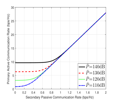
Figure 2: The asymptotic primary active communication rate versus secondary passive communication rate in SIMO symbiotic radio.

Fig. 2 gives an example plot of (32) with β_h_d=120subscript𝛽_subscript_𝑑120{{\beta}_{\_}{{{h}_{\_}{d}}}}=-120 dB, M_r=8subscript𝑀_𝑟8M_{\_}r=8 and K=128𝐾128K=128, for four different transmit SNR values P¯¯𝑃\bar{P}. It is worth mentioning that while (32) was derived for asymptotic setup with J1much-greater-than𝐽1J\gg 1, it is also applicable for the extreme case with J=0𝐽0J=0 or R_BDasym=0subscript𝑅_𝐵superscript𝐷asym0{R}_{\_}{BD}^{\mathrm{asym}}=0, for which case the third term inside the logarithm of (32) vanishes. Therefore, Fig. 2 plots R_sasymsubscript𝑅_superscript𝑠asym{R}_{\_}{s}^{\mathrm{asym}} versus R_BDasymsubscript𝑅_𝐵superscript𝐷asym{R}_{\_}{BD}^{\mathrm{asym}} in (32), starting from R_BDasym=0subscript𝑅_𝐵superscript𝐷asym0{R}_{\_}{BD}^{\mathrm{asym}}=0. It is observed from Fig. 2 that when the secondary passive communication rate is small, i.e., when J𝐽J is small and/or the cascaded channel αh_j𝐠_j𝛼subscript_𝑗subscript𝐠_𝑗\sqrt{\alpha}{{h}_{\_}{j}}{\mathbf{g}_{\_}j} is weak, increasing R_BDasymsubscript𝑅_𝐵superscript𝐷asym{R}_{\_}{BD}^{\mathrm{asym}} has a negligible impact on the primary active communication rate. However, once R_BDasymsubscript𝑅_𝐵superscript𝐷asym{R}_{\_}{BD}^{\mathrm{asym}} exceeds certain threshold, R_sasymsubscript𝑅_superscript𝑠asym{R}_{\_}{s}^{\mathrm{asym}} increases almost linearly with R_BDasymsubscript𝑅_𝐵superscript𝐷asym{R}_{\_}{BD}^{\mathrm{asym}}. This thus demonstrates that the mutualism of symbiotic radio can only be fully exploited for sufficiently large BDs. It is also interesting to observe that as R_BDasymsubscript𝑅_𝐵superscript𝐷asym{R}_{\_}{BD}^{\mathrm{asym}} becomes sufficiently large, R_sasymsubscript𝑅_superscript𝑠asym{R}_{\_}{s}^{\mathrm{asym}} for different P¯¯𝑃\bar{P} values merge. This can be verified by taking the derivative of R_sasymsubscript𝑅_superscript𝑠asym{R}_{\_}{s}^{\mathrm{asym}} in (32) with respect to P¯¯𝑃\bar{P}, which vanishes as R_BDasymsubscript𝑅_𝐵superscript𝐷asym{R}_{\_}{BD}^{\mathrm{asym}} gets sufficiently large.

V Precoding Optimization

In this section, for any given finite number of BDs J𝐽J where the asymptotic results in the previous section no longer hold, we consider the transmit precoding optimization problem to maximize the average primary communication rate in (3), under the sum rate constraint of the BDs in (14). The following problem can be formulated:

(P1)P1\displaystyle(\text{P}1)\quad\quad
max𝐅M_t×M_s,M_sM_t\displaystyle\underset{M_{\_}s\leq M_{\_}t}{\underset{\mathbf{F}\in\mathbb{C}^{M_{\_}t\times M_{\_}s},}{\mathop{\max}}}\, 𝔼_𝐜(n)[log_2|𝐈_M_r+P¯𝐇_eq(𝐜(n))𝐅𝐅H𝐇_eqH(𝐜(n))|]subscript𝔼_𝐜𝑛delimited-[]subscript_2subscript𝐈_subscript𝑀_𝑟¯𝑃subscript𝐇_𝑒𝑞𝐜𝑛superscript𝐅𝐅Hsubscript𝐇_𝑒superscript𝑞H𝐜𝑛\displaystyle{{\mathbb{E}}_{\_}{\mathbf{c}(n)}}\left[{{\log}_{\_}{2}}\left|{{\mathbf{I}}_{\_}{M_{\_}r}}+{\bar{P}}{{\mathbf{H}}_{\_}{eq}}\left(\mathbf{c}\left(n\right)\right)\mathbf{F}{{\mathbf{F}}^{\text{H}}}\mathbf{H}_{\_}{eq}^{\text{H}}\left(\mathbf{c}\left(n\right)\right)\right|\right] (33)
s.t.1Kformulae-sequencest1𝐾\displaystyle{\rm s.t.}\quad\frac{1}{K} log_2|𝐈_M_rM_s+KP¯α_j=1J((𝐅H𝐡_j𝐡_jH𝐅)(𝐠_j𝐠_jH)T)|\displaystyle{{\log}_{\_}{2}}\Big{|}{{\mathbf{I}}_{\_}{M_{\_}rM_{\_}s}}+{K\bar{P}\alpha}\sum\limits_{\_}{j=1}^{J}{\Big{(}\big{(}{{\mathbf{F}}^{\text{H}}}{{\mathbf{h}}_{\_}{j}}\mathbf{h}_{\_}{j}^{\text{H}}\mathbf{F}\big{)}\otimes{{\big{(}{{\mathbf{g}}_{\_}{j}}\mathbf{g}_{\_}{j}^{\text{H}}\big{)}}^{\text{T}}}\Big{)}}\Big{|}
r_BD,absentsubscript𝑟_𝐵𝐷\displaystyle\quad\quad\quad\quad\quad\quad\quad\quad\quad\quad\quad\quad\quad\quad\quad\quad\geq{{r}_{\_}{BD}}, (34)
trtr\displaystyle{\rm tr} (𝐅𝐅H)=1,superscript𝐅𝐅H1\displaystyle\big{(}\mathbf{F}{{\mathbf{F}}^{\text{H}}}\big{)}=1, (35)

where r_BDsubscript𝑟_𝐵𝐷{r}_{\_}{BD} denotes the given targeting threshold for the sum rate of the J𝐽J BDs. Note that the optimization variables in (P1) include the number of data streams M_ssubscript𝑀_𝑠M_{\_}s, as well as the precoding matrix 𝐅𝐅\mathbf{F}. Problem (P1) is non-convex, which is difficult to be directly solved. Fortunately, it can be transformed to an equivalent convex problem of optimizing the transmit covariance matrix. To this end, define 𝐐=𝐅𝐅H𝐐superscript𝐅𝐅H\mathbf{Q}=\mathbf{F}{{\mathbf{F}}^{\text{H}}}, which is the transmit covariance matrix of the PT. Then problem (P1) can be equivalently written as

(P1.1)P1.1\displaystyle(\text{P}1.1)\quad\quad
max𝐅M_t×M_s,𝐐,M_sM_t\displaystyle\underset{M_{\_}s\leq M_{\_}t}{\underset{\mathbf{F}\in\mathbb{C}^{M_{\_}t\times M_{\_}s},\mathbf{Q},}{\mathop{\max}}}\, 𝔼_𝐜(n)[log_2|𝐈_M_r+P¯𝐇_eq(𝐜(n))𝐐𝐇_eqH(𝐜(n))|]subscript𝔼_𝐜𝑛delimited-[]subscript_2subscript𝐈_subscript𝑀_𝑟¯𝑃subscript𝐇_𝑒𝑞𝐜𝑛subscript𝐐𝐇_𝑒superscript𝑞H𝐜𝑛\displaystyle{{\mathbb{E}}_{\_}{\mathbf{c}(n)}}\left[{{\log}_{\_}{2}}\left|{{\mathbf{I}}_{\_}{M_{\_}r}}+{\bar{P}}{{\mathbf{H}}_{\_}{eq}}\left(\mathbf{c}\left(n\right)\right)\mathbf{Q}\mathbf{H}_{\_}{eq}^{\text{H}}\left(\mathbf{c}\left(n\right)\right)\right|\right] (36)
s.t.1Kformulae-sequencest1𝐾\displaystyle{\rm s.t.}\quad\frac{1}{K} log_2|𝐈_M_rM_s+KP¯α_j=1J((𝐅H𝐡_j𝐡_jH𝐅)(𝐠_j𝐠_jH)T)|\displaystyle{{\log}_{\_}{2}}\Big{|}{{\mathbf{I}}_{\_}{M_{\_}rM_{\_}s}}+{K\bar{P}\alpha}\sum\limits_{\_}{j=1}^{J}{\Big{(}\big{(}{{\mathbf{F}}^{\text{H}}}{{\mathbf{h}}_{\_}{j}}\mathbf{h}_{\_}{j}^{\text{H}}\mathbf{F}\big{)}\otimes{{\big{(}{{\mathbf{g}}_{\_}{j}}\mathbf{g}_{\_}{j}^{\text{H}}\big{)}}^{\text{T}}}\Big{)}}\Big{|}
r_BD,absentsubscript𝑟_𝐵𝐷\displaystyle\quad\quad\quad\quad\quad\quad\quad\quad\quad\quad\quad\quad\quad\quad\quad\geq{{r}_{\_}{BD}}, (37)
trtr\displaystyle{\rm tr} (𝐐)=1,𝐐1\displaystyle(\mathbf{Q})=1, (38)
𝐐𝐐\displaystyle\mathbf{Q} =𝐅𝐅H.absentsuperscript𝐅𝐅H\displaystyle=\mathbf{F}{{\mathbf{F}}^{\text{H}}}. (39)

(P1.1) is still non-convex since the constraint (37) and (39) are non-convex. In the following, to find an equivalent convex transformation of (P1.1), we first consider the special case of one single BD, i.e., J=1𝐽1J=1, and then consider the more general case with J1𝐽1J\geq 1.

V-A Single BD: J=1𝐽1J=1

For the special case of single BD with J=1𝐽1J=1, the left hand side of (37) can be simplified as:

R_1=1Klog_2|𝐈_M_rM_s+KP¯α(𝐅H𝐡_1𝐡_1H𝐅)(𝐠_1𝐠_1H)T|=1Klog_2|𝐈_M_rM_s+KP¯α(𝐅H𝐡_1𝐠_1)(𝐡_1H𝐅𝐠_1T)|=1Klog_2(1+KP¯α(𝐡_1H𝐅𝐠_1T)(𝐅H𝐡_1𝐠_1))=1Klog_2(1+KP¯α𝐠_12𝐡_1H𝐅𝐅H𝐡_1),subscript𝑅_11𝐾subscript_2subscript𝐈_subscript𝑀_𝑟subscript𝑀_𝑠tensor-product𝐾¯𝑃𝛼superscript𝐅Hsubscript𝐡_1subscript𝐡_superscript1H𝐅superscriptsubscript𝐠_1subscript𝐠_superscript1HT1𝐾subscript_2subscript𝐈_subscript𝑀_𝑟subscript𝑀_𝑠𝐾¯𝑃𝛼tensor-productsuperscript𝐅Hsubscript𝐡_1subscript𝐠_superscript1tensor-productsubscript𝐡_superscript1H𝐅subscript𝐠_superscript1T1𝐾subscript_21𝐾¯𝑃𝛼tensor-productsubscript𝐡_superscript1H𝐅subscript𝐠_superscript1Ttensor-productsuperscript𝐅Hsubscript𝐡_1subscript𝐠_superscript11𝐾subscript_21𝐾¯𝑃𝛼superscriptdelimited-∥∥subscript𝐠_12subscript𝐡_superscript1Hsuperscript𝐅𝐅Hsubscript𝐡_1\begin{split}{{R}_{\_}{1}}&=\frac{1}{K}{{\log}_{\_}{2}}\left|{{\mathbf{I}}_{\_}{M_{\_}rM_{\_}s}}+{K\bar{P}\alpha}\left({{\mathbf{F}}^{\text{H}}}{{\mathbf{h}}_{\_}{1}}\mathbf{h}_{\_}{1}^{\text{H}}\mathbf{F}\right)\otimes{{\left({{\mathbf{g}}_{\_}{1}}\mathbf{g}_{\_}{1}^{\text{H}}\right)}^{\text{T}}}\right|\\ &=\frac{1}{K}{{\log}_{\_}{2}}\left|{{\mathbf{I}}_{\_}{M_{\_}rM_{\_}s}}+{K\bar{P}\alpha}\left({{\mathbf{F}}^{\text{H}}}{{\mathbf{h}}_{\_}{1}}\otimes\mathbf{g}_{\_}{1}^{*}\right)\left(\mathbf{h}_{\_}{1}^{\text{H}}\mathbf{F}\otimes\mathbf{g}_{\_}{1}^{\text{T}}\right)\right|\\ &=\frac{1}{K}{{\log}_{\_}{2}}\left(1+{K\bar{P}\alpha}\left(\mathbf{h}_{\_}{1}^{\text{H}}\mathbf{F}\otimes\mathbf{g}_{\_}{1}^{\text{T}}\right)\left({{\mathbf{F}}^{\text{H}}}{{\mathbf{h}}_{\_}{1}}\otimes\mathbf{g}_{\_}{1}^{*}\right)\right)\\ &=\frac{1}{K}{{\log}_{\_}{2}}\left(1+{K\bar{P}\alpha{{\left\|{{\mathbf{g}}_{\_}{1}}\right\|}^{2}}\mathbf{h}_{\_}{1}^{\text{H}}\mathbf{F}{{\mathbf{F}}^{\text{H}}}{{\mathbf{h}}_{\_}{1}}}\right),\end{split} (40)

where the second and last equalities follow from the identity (𝐀𝐁)(𝐂𝐃)=𝐀𝐂𝐁𝐃tensor-product𝐀𝐁tensor-product𝐂𝐃tensor-product𝐀𝐂𝐁𝐃\left(\mathbf{A}\otimes\mathbf{B}\right)\left(\mathbf{C}\otimes\mathbf{D}\right)=\mathbf{AC}\otimes\mathbf{BD}, and the third equality follows from the Weinstein-Aronszajn identity |𝐈_m+𝐀𝐁|=|𝐈_n+𝐁𝐀|subscript𝐈_𝑚𝐀𝐁subscript𝐈_𝑛𝐁𝐀\left|{{\mathbf{I}}_{\_}{m}}+\mathbf{AB}\right|=\left|{{\mathbf{I}}_{\_}{n}}+\mathbf{BA}\right|. By substituting (40) and 𝐐=𝐅𝐅H𝐐superscript𝐅𝐅H\mathbf{Q}=\mathbf{F}{{\mathbf{F}}^{\text{H}}} into the left hand side of (37), (P1.1) can be transformed to:

(P2)P2\displaystyle(\text{P}2)\quad
max𝐐𝐐\displaystyle\underset{\mathbf{Q}}{\mathop{\max}}\quad 𝔼_𝐜(n)[log_2|𝐈_M_r+P¯𝐇_eq(𝐜(n))𝐐𝐇_eqH(𝐜(n))|]subscript𝔼_𝐜𝑛delimited-[]subscript_2subscript𝐈_subscript𝑀_𝑟¯𝑃subscript𝐇_𝑒𝑞𝐜𝑛subscript𝐐𝐇_𝑒superscript𝑞H𝐜𝑛\displaystyle{{\mathbb{E}}_{\_}{\mathbf{c}(n)}}\left[{{\log}_{\_}{2}}\left|{{\mathbf{I}}_{\_}{M_{\_}r}}+{\bar{P}}{{\mathbf{H}}_{\_}{eq}}\left(\mathbf{c}\left(n\right)\right)\mathbf{QH}_{\_}{eq}^{\text{H}}\left(\mathbf{c}\left(n\right)\right)\right|\right] (41)
s.t.formulae-sequencest\displaystyle{\rm s.t.}\quad 1Klog_2(1+KP¯α𝐠_12𝐡_1H𝐐𝐡_1)r_BD,1𝐾subscript_21𝐾¯𝑃𝛼superscriptnormsubscript𝐠_12subscript𝐡_superscript1Hsubscript𝐐𝐡_1subscript𝑟_𝐵𝐷\displaystyle\frac{1}{K}{{\log}_{\_}{2}}\left(1+{K\bar{P}\alpha{{\left\|{{\mathbf{g}}_{\_}{1}}\right\|}^{2}}\mathbf{h}_{\_}{1}^{\text{H}}\mathbf{Q}{{\mathbf{h}}_{\_}{1}}}\right)\geq{{r}_{\_}{BD}}, (42)
tr(𝐐)=1,𝐐0.formulae-sequencetr𝐐1succeeds-or-equals𝐐0\displaystyle{\rm tr}(\mathbf{Q})=1,\mathbf{Q}\succeq 0. (43)

Note that in (P2), the only optimization variable is the transmit covariance matrix 𝐐𝐐\mathbf{Q}, and we have temporarily removed the constraints 𝐐=𝐅𝐅H𝐐superscript𝐅𝐅H\mathbf{Q}=\mathbf{F}{{\mathbf{F}}^{\text{H}}}, 𝐅M_t×M_s𝐅superscriptsubscript𝑀_𝑡subscript𝑀_𝑠\mathbf{F}\in\mathbb{C}^{M_{\_}t\times M_{\_}s}, and M_sM_tsubscript𝑀_𝑠subscript𝑀_𝑡M_{\_}s\leq M_{\_}t. This does not affect the equivalence between P(1.1) and (P2), since once the optimal transmit covariance matrix 𝐐superscript𝐐\mathbf{Q}^{\star} to (P2) is obtained, we can always find the corresponding precoding matrix 𝐅𝐅\mathbf{F} and the number of data streams M_ssubscript𝑀_𝑠M_{\_}s satisfying the constraint of (P1.1). One straightforward method is by applying eigenvalue decomposition to 𝐐superscript𝐐\mathbf{Q}^{\star}. Specifically, let the (reduced) EVD of 𝐐superscript𝐐\mathbf{Q}^{\star} be 𝐐=𝐔𝚺𝐔Hsuperscript𝐐𝐔𝚺superscript𝐔H\mathbf{Q}^{\star}=\mathbf{U\Sigma}{{\mathbf{U}}^{\text{H}}}, where 𝐔M_t×r𝐔superscriptsubscript𝑀_𝑡𝑟\mathbf{U}\in{{\mathbb{C}}^{{{M}_{\_}{t}}\times r}} is a semi-unitary matrix and 𝚺𝚺\mathbf{\Sigma} is an r×r𝑟𝑟r\times r diagonal matrix whose diagonal elements are the positive eigenvalues of 𝐐superscript𝐐\mathbf{Q}^{\star}, and rM_t𝑟subscript𝑀_𝑡r\leq M_{\_}t is the rank of 𝐐superscript𝐐\mathbf{Q}^{\star}.Then, to find M_ssubscript𝑀_𝑠M_{\_}s and 𝐅𝐅\mathbf{F} that are feasible to (P1.1), we may simply let M_s=rsubscript𝑀_𝑠𝑟M_{\_}s=r, and 𝐅=𝐔𝚺1/2𝐅𝐔superscript𝚺12{\mathbf{F}}=\mathbf{U}\mathbf{\Sigma}^{1/2}. Obviously, the corresponding solution is optimal to (P1.1) since it achieves the same optimal value as its relaxed problem (P2). Therefore, the remaining task is to solve (P2) by optimizing the transmit covariance matrix 𝐐𝐐\mathbf{Q}. It is not difficult to see that (P2) is a convex optimization problem, which in principle can be solved by standard convex optimization techniques. However, the difficulty lies in that the objective function of (P2) involves an expectation with respect to the random BD symbols 𝐜(n)𝐜𝑛\mathbf{c}(n). To tackle this issue, we will approximate (41) by its sample average or upper bound, and convert the problem into a more tractable convex optimization problem. The details will be presented in Subsection IV B, since similar techniques will also be used for the general case with multiple BDs presented in the next subsection.

V-B Multiple BDs: J1𝐽1J\geq 1

In this subsection, we consider the general case of (P1.1) with multiple BDs. In this case, by using Theorem 1, the left hand side of (37) can be equivalently expressed as (13). Define 𝐗=[𝐱_1,𝐱_2,,𝐱_J]𝐗subscript𝐱_1subscript𝐱_2subscript𝐱_𝐽\mathbf{X}=\left[{{\mathbf{x}}_{\_}{1}},{{\mathbf{x}}_{\_}{2}},\cdots,{{\mathbf{x}}_{\_}{J}}\right], we have

R_BD=1Klog_2|𝐈_M_rM_s+1σ2_j=1J𝐱_j𝐱_jH|=1Klog_2|𝐈_M_rM_s+1σ2𝐗𝐗H|=1Klog_2|𝐈_J+1σ2𝐗H𝐗|=1Klog_2|𝐈_J+1σ2𝐗T𝐗|,\begin{split}{{R}_{\_}{BD}}&=\frac{1}{K}{{\log}_{\_}{2}}\Big{|}{{\mathbf{I}}_{\_}{M_{\_}rM_{\_}s}}+\frac{1}{{{\sigma}^{2}}}\sum\limits_{\_}{j=1}^{J}{{{\mathbf{x}}_{\_}{j}}\mathbf{x}_{\_}{j}^{\text{H}}}\Big{|}\\ &=\frac{1}{K}{{\log}_{\_}{2}}\Big{|}{{\mathbf{I}}_{\_}{M_{\_}rM_{\_}s}}+\frac{1}{{{\sigma}^{2}}}\mathbf{X}{{\mathbf{X}}^{\text{H}}}\Big{|}\\ &=\frac{1}{K}{{\log}_{\_}{2}}\Big{|}{{\mathbf{I}}_{\_}{J}}+\frac{1}{{{\sigma}^{2}}}{{\mathbf{X}}^{\text{H}}}\mathbf{X}\Big{|}\\ &=\frac{1}{K}{{\log}_{\_}{2}}\Big{|}{{\mathbf{I}}_{\_}{J}}+\frac{1}{{{\sigma}^{2}}}{{\mathbf{X}}^{\text{T}}}{{\mathbf{X}}^{*}}\Big{|},\end{split} (44)

where the second last equality follows from the Weinstein-Aronszajn identity |𝐈_m+𝐀𝐁|=|𝐈_n+𝐁𝐀|subscript𝐈_𝑚𝐀𝐁subscript𝐈_𝑛𝐁𝐀\left|{{\mathbf{I}}_{\_}{m}}+\mathbf{AB}\right|=\left|{{\mathbf{I}}_{\_}{n}}+\mathbf{BA}\right|, and the last equality follows from the identity |𝐀T|=|𝐀|superscript𝐀T𝐀\left|{{\mathbf{A}}^{\text{T}}}\right|=\left|\mathbf{A}\right|. By using the identity vec(𝐀_1𝐀_2𝐀_3)=(𝐀_3T𝐀_1)vec(𝐀_2)vecsubscript𝐀_1subscript𝐀_2subscript𝐀_3tensor-productsubscript𝐀_superscript3Tsubscript𝐀_1vecsubscript𝐀_2\text{vec}({{\mathbf{A}}_{\_}{1}}{{\mathbf{A}}_{\_}{2}}{{\mathbf{A}}_{\_}{3}})=\left(\mathbf{A}_{\_}{3}^{\text{T}}\otimes{{\mathbf{A}}_{\_}{1}}\right)\text{vec}({{\mathbf{A}}_{\_}{2}}), we have

𝐱_j=vec(KPα𝐠_j𝐡_jH𝐅)=KPα(𝐅T𝐠_j𝐡_jH)vec(𝐈_M_t).subscript𝐱_𝑗vec𝐾𝑃𝛼subscript𝐠_𝑗subscript𝐡_superscript𝑗H𝐅𝐾𝑃𝛼tensor-productsuperscript𝐅Tsubscript𝐠_𝑗subscript𝐡_superscript𝑗Hvecsubscript𝐈_subscript𝑀_𝑡\begin{split}{{\mathbf{x}}_{\_}{j}}&=\text{vec}\left(\sqrt{KP\alpha}{{\mathbf{g}}_{\_}{j}}\mathbf{h}_{\_}{j}^{\text{H}}\mathbf{F}\right)\\ &=\sqrt{KP\alpha}\left({{\mathbf{F}}^{\text{T}}}\otimes{{\mathbf{g}}_{\_}{j}}\mathbf{h}_{\_}{j}^{\text{H}}\right)\text{vec}\left({{\mathbf{I}}_{\_}{M_{\_}t}}\right).\end{split} (45)

Then 𝐗𝐗\mathbf{X} can be expressed as (46) shown at the top of the next page.

𝐗=KPα[(𝐅T𝐠_1𝐡_1H)vec(𝐈_M_t),(𝐅T𝐠_2𝐡_2H)vec(𝐈_M_t),,(𝐅T𝐠_J𝐡_JH)vec(𝐈_M_t)]=KPα[(𝐅T𝐠_1𝐡_1H),(𝐅T𝐠_2𝐡_2H),,(𝐅T𝐠_J𝐡_JH)][vec(𝐈_M_t)𝟎𝟎𝟎vec(𝐈_M_t)𝟎𝟎𝟎vec(𝐈_M_t)]=KPα(𝐅T[𝐠_1𝐡_1H,𝐠_2𝐡_2H,,𝐠_J𝐡_JH])[vec(𝐈_M_t)𝟎𝟎𝟎vec(𝐈_M_t)𝟎𝟎𝟎vec(𝐈_M_t)]𝐗𝐾𝑃𝛼tensor-productsuperscript𝐅Tsubscript𝐠_1subscript𝐡_superscript1Hvecsubscript𝐈_subscript𝑀_𝑡tensor-productsuperscript𝐅Tsubscript𝐠_2subscript𝐡_superscript2Hvecsubscript𝐈_subscript𝑀_𝑡tensor-productsuperscript𝐅Tsubscript𝐠_𝐽subscript𝐡_superscript𝐽Hvecsubscript𝐈_subscript𝑀_𝑡𝐾𝑃𝛼tensor-productsuperscript𝐅Tsubscript𝐠_1subscript𝐡_superscript1Htensor-productsuperscript𝐅Tsubscript𝐠_2subscript𝐡_superscript2Htensor-productsuperscript𝐅Tsubscript𝐠_𝐽subscript𝐡_superscript𝐽Hdelimited-[]matrixvecsubscript𝐈_subscript𝑀_𝑡000vecsubscript𝐈_subscript𝑀_𝑡000vecsubscript𝐈_subscript𝑀_𝑡𝐾𝑃𝛼tensor-productsuperscript𝐅Tsubscript𝐠_1subscript𝐡_superscript1Hsubscript𝐠_2subscript𝐡_superscript2Hsubscript𝐠_𝐽subscript𝐡_superscript𝐽Hdelimited-[]matrixvecsubscript𝐈_subscript𝑀_𝑡000vecsubscript𝐈_subscript𝑀_𝑡000vecsubscript𝐈_subscript𝑀_𝑡\begin{split}\mathbf{X}&=\sqrt{KP\alpha}\left[\left({{\mathbf{F}}^{\text{T}}}\otimes{{\mathbf{g}}_{\_}{1}}\mathbf{h}_{\_}{1}^{\text{H}}\right)\text{vec}\left({{\mathbf{I}}_{\_}{M_{\_}t}}\right),\left({{\mathbf{F}}^{\text{T}}}\otimes{{\mathbf{g}}_{\_}{2}}\mathbf{h}_{\_}{2}^{\text{H}}\right)\text{vec}\left({{\mathbf{I}}_{\_}{M_{\_}t}}\right),\cdots,\left({{\mathbf{F}}^{\text{T}}}\otimes{{\mathbf{g}}_{\_}{J}}\mathbf{h}_{\_}{J}^{\text{H}}\right)\text{vec}\left({{\mathbf{I}}_{\_}{M_{\_}t}}\right)\right]\\ &=\sqrt{KP\alpha}\left[\left({{\mathbf{F}}^{\text{T}}}\otimes{{\mathbf{g}}_{\_}{1}}\mathbf{h}_{\_}{1}^{\text{H}}\right),\left({{\mathbf{F}}^{\text{T}}}\otimes{{\mathbf{g}}_{\_}{2}}\mathbf{h}_{\_}{2}^{\text{H}}\right),\cdots,\left({{\mathbf{F}}^{\text{T}}}\otimes{{\mathbf{g}}_{\_}{J}}\mathbf{h}_{\_}{J}^{\text{H}}\right)\right]\left[\begin{matrix}\text{vec}\left({{\mathbf{I}}_{\_}{M_{\_}t}}\right)&{\mathbf{0}}&\cdots&{\mathbf{0}}\\ {\mathbf{0}}&\text{vec}\left({{\mathbf{I}}_{\_}{M_{\_}t}}\right)&\cdots&{\mathbf{0}}\\ \vdots&\vdots&\ddots&\vdots\\ {\mathbf{0}}&{\mathbf{0}}&\cdots&\text{vec}\left({{\mathbf{I}}_{\_}{M_{\_}t}}\right)\\ \end{matrix}\right]\\ &=\sqrt{KP\alpha}\left({{\mathbf{F}}^{\text{T}}}\otimes\left[{{\mathbf{g}}_{\_}{1}}\mathbf{h}_{\_}{1}^{\text{H}},{{\mathbf{g}}_{\_}{2}}\mathbf{h}_{\_}{2}^{\text{H}},\cdots,{{\mathbf{g}}_{\_}{J}}\mathbf{h}_{\_}{J}^{\text{H}}\right]\right)\left[\begin{matrix}\text{vec}\left({{\mathbf{I}}_{\_}{M_{\_}t}}\right)&{\mathbf{0}}&\cdots&{\mathbf{0}}\\ {\mathbf{0}}&\text{vec}\left({{\mathbf{I}}_{\_}{M_{\_}t}}\right)&\cdots&{\mathbf{0}}\\ \vdots&\vdots&\ddots&\vdots\\ {\mathbf{0}}&{\mathbf{0}}&\cdots&\text{vec}\left({{\mathbf{I}}_{\_}{M_{\_}t}}\right)\\ \end{matrix}\right]\end{split} (46)

For notational convenience, we let 𝐇=[𝐠_1𝐡_1H,𝐠_2𝐡_2H,,𝐠_J𝐡_JH]M_r×M_tJ𝐇subscript𝐠_1subscript𝐡_superscript1Hsubscript𝐠_2subscript𝐡_superscript2Hsubscript𝐠_𝐽subscript𝐡_superscript𝐽Hsuperscriptsubscript𝑀_𝑟subscript𝑀_𝑡𝐽\mathbf{H}=\left[{{\mathbf{g}}_{\_}{1}}\mathbf{h}_{\_}{1}^{\text{H}},{{\mathbf{g}}_{\_}{2}}\mathbf{h}_{\_}{2}^{\text{H}},\cdots,{{\mathbf{g}}_{\_}{J}}\mathbf{h}_{\_}{J}^{\text{H}}\right]\in{{\mathbb{C}}^{M_{\_}r\times M_{\_}tJ}} and

𝚿=[vec(𝐈_M_t)𝟎𝟎𝟎vec(𝐈_M_t)𝟎𝟎𝟎vec(𝐈_M_t)]M_t2J×J,𝚿delimited-[]matrixvecsubscript𝐈_subscript𝑀_𝑡000vecsubscript𝐈_subscript𝑀_𝑡000vecsubscript𝐈_subscript𝑀_𝑡superscriptsubscript𝑀_superscript𝑡2𝐽𝐽\mathbf{\Psi}=\left[\begin{matrix}\text{vec}\left({{\mathbf{I}}_{\_}{M_{\_}t}}\right)&{\mathbf{0}}&\cdots&{\mathbf{0}}\\ {\mathbf{0}}&\text{vec}\left({{\mathbf{I}}_{\_}{M_{\_}t}}\right)&\cdots&{\mathbf{0}}\\ \vdots&\vdots&\ddots&\vdots\\ {\mathbf{0}}&{\mathbf{0}}&\cdots&\text{vec}\left({{\mathbf{I}}_{\_}{M_{\_}t}}\right)\\ \end{matrix}\right]\in{{\mathbb{R}}^{M_{\_}t^{2}J\times J}}, (47)

so that 𝐗=KPα(𝐅T𝐇)𝚿𝐗𝐾𝑃𝛼tensor-productsuperscript𝐅T𝐇𝚿\mathbf{X}=\sqrt{KP\alpha}\left({{\mathbf{F}}^{\text{T}}}\otimes\mathbf{H}\right)\mathbf{\Psi}. Then R_BDsubscript𝑅_𝐵𝐷R_{\_}{BD} in (44) can be expressed as

R_BD=1Klog_2|𝐈_J+1σ2𝐗T𝐗|=1Klog_2|𝐈_J+KP¯α𝚿T(𝐅T𝐇)T(𝐅T𝐇)𝚿|=1Klog_2|𝐈_J+KP¯α𝚿H(𝐅𝐅H(𝐇H𝐇)T)𝚿|,subscript𝑅_𝐵𝐷1𝐾subscript_2subscript𝐈_𝐽1superscript𝜎2superscript𝐗Tsuperscript𝐗1𝐾subscript_2subscript𝐈_𝐽𝐾¯𝑃𝛼superscript𝚿Tsuperscripttensor-productsuperscript𝐅T𝐇Tsuperscripttensor-productsuperscript𝐅T𝐇superscript𝚿1𝐾subscript_2subscript𝐈_𝐽𝐾¯𝑃𝛼superscript𝚿Htensor-productsuperscript𝐅𝐅Hsuperscriptsuperscript𝐇H𝐇T𝚿\begin{split}{{R}_{\_}{BD}}&=\frac{1}{K}{{\log}_{\_}{2}}\Big{|}{{\mathbf{I}}_{\_}{J}}+\frac{1}{{{\sigma}^{2}}}{{\mathbf{X}}^{\text{T}}}{{\mathbf{X}}^{*}}\Big{|}\\ &=\frac{1}{K}{{\log}_{\_}{2}}\Big{|}{{\mathbf{I}}_{\_}{J}}+{K\bar{P}\alpha}{{\mathbf{\Psi}}^{\text{T}}}{{\left({{\mathbf{F}}^{\text{T}}}\otimes\mathbf{H}\right)}^{\text{T}}}{{\left({{\mathbf{F}}^{\text{T}}}\otimes\mathbf{H}\right)}^{*}}{{\mathbf{\Psi}}^{*}}\Big{|}\\ &=\frac{1}{K}{{\log}_{\_}{2}}\Big{|}{{\mathbf{I}}_{\_}{J}}+{K\bar{P}\alpha}{{\mathbf{\Psi}}^{\text{H}}}\left(\mathbf{F}{{\mathbf{F}}^{\text{H}}}\otimes{{\left({{\mathbf{H}}^{\text{H}}}\mathbf{H}\right)}^{\text{T}}}\right)\mathbf{\Psi}\Big{|},\\ \end{split} (48)

where the last equality follows from the identities (𝐀𝐁)T=𝐀T𝐁Tsuperscripttensor-product𝐀𝐁Ttensor-productsuperscript𝐀Tsuperscript𝐁T{{\left(\mathbf{A}\otimes\mathbf{B}\right)}^{\text{T}}}={{\mathbf{A}}^{\text{T}}}\otimes{{\mathbf{B}}^{\text{T}}}, (𝐀𝐁)=𝐀𝐁superscripttensor-product𝐀𝐁tensor-productsuperscript𝐀superscript𝐁{{\left(\mathbf{A}\otimes\mathbf{B}\right)}^{*}}={{\mathbf{A}}^{*}}\otimes{{\mathbf{B}}^{*}}, (𝐀𝐁)(𝐂𝐃)=𝐀𝐂𝐁𝐃tensor-product𝐀𝐁tensor-product𝐂𝐃tensor-product𝐀𝐂𝐁𝐃\left(\mathbf{A}\otimes\mathbf{B}\right)\left(\mathbf{C}\otimes\mathbf{D}\right)=\mathbf{AC}\otimes\mathbf{BD} and 𝚿𝚿\mathbf{\Psi}\in{\mathbb{R}}. When J=1𝐽1J=1, 𝐇=𝐠_1𝐡_1H𝐇subscript𝐠_1subscript𝐡_superscript1H\mathbf{H}={{\mathbf{g}}_{\_}{1}}\mathbf{h}_{\_}{1}^{\text{H}}, 𝚿=vec(𝐈_M_t)𝚿vecsubscript𝐈_subscript𝑀_𝑡\mathbf{\Psi}=\text{vec}\left({{\mathbf{I}}_{\_}{{{M}_{\_}{t}}}}\right), (LABEL:eq:RBDnew) can be simplified to (40). By replacing R_BDsubscript𝑅_𝐵𝐷R_{\_}{BD} in (37) with (LABEL:eq:RBDnew) and letting 𝐐=𝐅𝐅H𝐐superscript𝐅𝐅H\mathbf{Q}=\mathbf{F}{{\mathbf{F}}^{\text{H}}}, we transform (P1.1) into

(P3)P3\displaystyle(\text{P}3)\quad
max𝐐𝐐\displaystyle\underset{\mathbf{Q}}{\mathop{\max}}\quad 𝔼_𝐜(n)[log_2|𝐈_M_r+P¯𝐇_eq(𝐜(n))𝐐𝐇_eqH(𝐜(n))|]subscript𝔼_𝐜𝑛delimited-[]subscript_2subscript𝐈_subscript𝑀_𝑟¯𝑃subscript𝐇_𝑒𝑞𝐜𝑛subscript𝐐𝐇_𝑒superscript𝑞H𝐜𝑛\displaystyle{{\mathbb{E}}_{\_}{\mathbf{c}(n)}}\left[{{\log}_{\_}{2}}\left|{{\mathbf{I}}_{\_}{M_{\_}r}}+{\bar{P}}{{\mathbf{H}}_{\_}{eq}}\left(\mathbf{c}\left(n\right)\right)\mathbf{QH}_{\_}{eq}^{\text{H}}\left(\mathbf{c}\left(n\right)\right)\right|\right] (49)
s.t.formulae-sequencest\displaystyle{\rm s.t.}\quad 1Klog_2|𝐈_J+KP¯α𝚿H(𝐐(𝐇H𝐇)T)𝚿|r_BD,1𝐾subscript_2subscript𝐈_𝐽𝐾¯𝑃𝛼superscript𝚿Htensor-product𝐐superscriptsuperscript𝐇H𝐇T𝚿subscript𝑟_𝐵𝐷\displaystyle\frac{1}{K}{{\log}_{\_}{2}}\Big{|}{{\mathbf{I}}_{\_}{J}}+{K\bar{P}\alpha}{{\mathbf{\Psi}}^{\text{H}}}\Big{(}\mathbf{Q}\otimes{{\left({{\mathbf{H}}^{\text{H}}}\mathbf{H}\right)}^{\text{T}}}\Big{)}\mathbf{\Psi}\Big{|}\geq{{r}_{\_}{BD}}, (50)
tr(𝐐)=1,𝐐0.formulae-sequencetr𝐐1succeeds-or-equals𝐐0\displaystyle{\rm tr}(\mathbf{Q})=1,\mathbf{Q}\succeq 0. (51)

After solving (P3), we can obtain 𝐅𝐅\mathbf{F} by using the same way as discussed in Subsection V A.

Note that similar to (P2), the transmit covariance matrix 𝐐𝐐\mathbf{Q} in (P3) is optimized to maximize the expected primary communication rate, with the expectation taken with respect to the random BD symbols 𝐜(n)𝐜𝑛\mathbf{c}(n). In the following, we propose two solution approaches to (P3), termed sample-average based solution and upper bound based solution, which have different trade-offs on performance and computational complexity.

V-B1 Sample-Average Based Solution

For the sample-average based solution, the expectation of the primary communication rate in (49) is approximated by its sample average. Specifically, let 𝐜_s,s=1,,Sformulae-sequencesubscript𝐜_𝑠𝑠1𝑆\mathbf{c}_{\_}s,s=1,...,S be S𝑆S independent realizations of 𝐜(n)𝐜𝑛\mathbf{c}(n) following its distribution f(𝐜(n))𝑓𝐜𝑛f(\mathbf{c}(n)). Then when S𝑆S is sufficiently large, based on the law of large numbers, (P3) can be approximated as

(P4)P4\displaystyle(\text{P}4)\quad
max𝐐𝐐\displaystyle\underset{\mathbf{Q}}{\mathop{\max}}\quad 1S_s=1Slog_2|𝐈_M_r+P¯𝐇_eq(𝐜_s)𝐐𝐇_eqH(𝐜_s)|1𝑆subscript_𝑠superscript1𝑆subscript_2subscript𝐈_subscript𝑀_𝑟¯𝑃subscript𝐇_𝑒𝑞subscript𝐜_𝑠subscript𝐐𝐇_𝑒superscript𝑞Hsubscript𝐜_𝑠\displaystyle\frac{1}{S}\sum\limits_{\_}{s=1}^{S}{{\log}_{\_}{2}}\left|{{\mathbf{I}}_{\_}{M_{\_}r}}+{\bar{P}}{{\mathbf{H}}_{\_}{eq}}\left({\mathbf{c}}_{\_}{s}\right)\mathbf{QH}_{\_}{eq}^{\text{H}}\left({\mathbf{c}}_{\_}{s}\right)\right| (52)
s.t.formulae-sequencest\displaystyle{\rm s.t.}\quad 1Klog_2|𝐈_J+KP¯α𝚿H(𝐐(𝐇H𝐇)T)𝚿|r_BD,1𝐾subscript_2subscript𝐈_𝐽𝐾¯𝑃𝛼superscript𝚿Htensor-product𝐐superscriptsuperscript𝐇H𝐇T𝚿subscript𝑟_𝐵𝐷\displaystyle\frac{1}{K}{{\log}_{\_}{2}}\Big{|}{{\mathbf{I}}_{\_}{J}}+{K\bar{P}\alpha}{{\mathbf{\Psi}}^{\text{H}}}\Big{(}\mathbf{Q}\otimes{{\left({{\mathbf{H}}^{\text{H}}}\mathbf{H}\right)}^{\text{T}}}\Big{)}\mathbf{\Psi}\Big{|}\geq{{r}_{\_}{BD}}, (53)
tr(𝐐)=1,𝐐0.formulae-sequencetr𝐐1succeeds-or-equals𝐐0\displaystyle{\rm tr}(\mathbf{Q})=1,\mathbf{Q}\succeq 0. (54)

(P4) is a convex optimization problem, which can be optimally solved by using software tools like CVX [39].

V-B2 Upper Bound Based Solution

Note that the above sample average based method needs to collect a large number of samples for the random state 𝐜(n)𝐜𝑛\mathbf{c}(n) before solving the stochastic optimization problem. Hence, it requires huge memory to store the samples and the corresponding computational complexity is also high. To address such issues, we substitute (49) with its upper bound and convert the problem into a more tractable convex problem. By using Jensen’s inequality, an upper bound of R_ssubscript𝑅_𝑠R_{\_}s in (49) is given by

R_s=𝔼_𝐜(n)[log_2|𝐈_M_t+P¯𝐐𝐇_eqH(𝐜(n))𝐇_eq(𝐜(n))|]R_sUBlog_2|𝐈_M_t+P¯𝐐𝔼_𝐜(n)[𝐇_eqH(𝐜(n))𝐇_eq(𝐜(n))]|,subscript𝑅_𝑠subscript𝔼_𝐜𝑛delimited-[]subscript_2subscript𝐈_subscript𝑀_𝑡¯𝑃subscript𝐐𝐇_𝑒superscript𝑞H𝐜𝑛subscript𝐇_𝑒𝑞𝐜𝑛subscript𝑅_𝑠𝑈𝐵subscript_2subscript𝐈_subscript𝑀_𝑡¯𝑃𝐐subscript𝔼_𝐜𝑛delimited-[]subscript𝐇_𝑒superscript𝑞H𝐜𝑛subscript𝐇_𝑒𝑞𝐜𝑛\begin{split}&{{R}_{\_}{s}}={{\mathbb{E}}_{\_}{\mathbf{c}(n)}}\left[{{\log}_{\_}{2}}\left|{{\mathbf{I}}_{\_}{{{M}_{\_}{t}}}}+{\bar{P}}\mathbf{QH}_{\_}{eq}^{\text{H}}\left(\mathbf{c}\left(n\right)\right){{\mathbf{H}}_{\_}{eq}}\left(\mathbf{c}\left(n\right)\right)\right|\right]\\ &\leq{{R}_{\_}{sUB}}\triangleq{{\log}_{\_}{2}}\left|{{\mathbf{I}}_{\_}{{{M}_{\_}{t}}}}+{\bar{P}}\mathbf{Q}{{\mathbb{E}}_{\_}{\mathbf{c}(n)}}\left[\mathbf{H}_{\_}{eq}^{\text{H}}\left(\mathbf{c}\left(n\right)\right){{\mathbf{H}}_{\_}{eq}}\left(\mathbf{c}\left(n\right)\right)\right]\right|,\\ \end{split} (55)

where

𝔼_𝐜(n)[𝐇_eqH(𝐜(n))𝐇_eq(𝐜(n))]=𝔼_𝐜(n)[(𝐇_d+_j=1Jα𝐠_j𝐡_jHc_j(n))H(𝐇_d+_j=1Jα𝐠_j𝐡_jHc_j(n))]=𝐇_dH𝐇_d+α𝔼_𝐜(n)[_j=1J_i=1Jc_j(n)c_i(n)𝐡_j𝐠_jH𝐠_i𝐡_iH]=𝐇_dH𝐇_d+α_j=1J𝐠_j2𝐡_j𝐡_jH.subscript𝔼_𝐜𝑛delimited-[]subscript𝐇_𝑒superscript𝑞H𝐜𝑛subscript𝐇_𝑒𝑞𝐜𝑛subscript𝔼_𝐜𝑛delimited-[]superscriptsubscript𝐇_𝑑subscript_𝑗superscript1𝐽𝛼subscript𝐠_𝑗subscript𝐡_superscript𝑗Hsubscript𝑐_𝑗𝑛Hsubscript𝐇_𝑑subscript_𝑗superscript1𝐽𝛼subscript𝐠_𝑗subscript𝐡_superscript𝑗Hsubscript𝑐_𝑗𝑛subscript𝐇_superscript𝑑Hsubscript𝐇_𝑑𝛼subscript𝔼_𝐜𝑛delimited-[]subscript_𝑗superscript1𝐽subscript_𝑖superscript1𝐽subscript𝑐_superscript𝑗𝑛subscript𝑐_𝑖𝑛subscript𝐡_𝑗subscript𝐠_superscript𝑗Hsubscript𝐠_𝑖subscript𝐡_superscript𝑖Hsubscript𝐇_superscript𝑑Hsubscript𝐇_𝑑𝛼subscript_𝑗superscript1𝐽superscriptdelimited-∥∥subscript𝐠_𝑗2subscript𝐡_𝑗subscript𝐡_superscript𝑗H\begin{split}&{{\mathbb{E}}_{\_}{\mathbf{c}(n)}}\left[\mathbf{H}_{\_}{eq}^{\text{H}}\left(\mathbf{c}\left(n\right)\right){{\mathbf{H}}_{\_}{eq}}\left(\mathbf{c}\left(n\right)\right)\right]\\ &={{\mathbb{E}}_{\_}{\mathbf{c}(n)}}\Big{[}{{\Big{(}{{\mathbf{H}}_{\_}{d}}+\sum\limits_{\_}{j=1}^{J}{\sqrt{\alpha}}{{\mathbf{g}}_{\_}{j}}\mathbf{h}_{\_}{j}^{\text{H}}{{c}_{\_}{j}}(n)\Big{)}}^{\text{H}}}\Big{(}{{\mathbf{H}}_{\_}{d}}+\sum\limits_{\_}{j=1}^{J}{\sqrt{\alpha}}{{\mathbf{g}}_{\_}{j}}\mathbf{h}_{\_}{j}^{\text{H}}{{c}_{\_}{j}}(n)\Big{)}\Big{]}\\ &=\mathbf{H}_{\_}{d}^{\text{H}}{{\mathbf{H}}_{\_}{d}}+\alpha{{\mathbb{E}}_{\_}{\mathbf{c}(n)}}\Big{[}\sum\limits_{\_}{j=1}^{J}{\sum\limits_{\_}{i=1}^{J}{c_{\_}{j}^{*}(n){{c}_{\_}{i}}(n)}}{{\mathbf{h}}_{\_}{j}}\mathbf{g}_{\_}{j}^{\text{H}}{{\mathbf{g}}_{\_}{i}}\mathbf{h}_{\_}{i}^{\text{H}}\Big{]}\\ &=\mathbf{H}_{\_}{d}^{\text{H}}{{\mathbf{H}}_{\_}{d}}+\alpha\sum\limits_{\_}{j=1}^{J}{{{\left\|{{\mathbf{g}}_{\_}{j}}\right\|}^{2}}{{\mathbf{h}}_{\_}{j}}}\mathbf{h}_{\_}{j}^{\text{H}}.\\ \end{split} (56)

The last equality of (56) follows since c(n)𝑐𝑛c(n) are i.i.d. random symbols for different BDs j𝑗j. Therefore, by replacing R_ssubscript𝑅_𝑠R_{\_}s in (49) with (55), we have

(P5)P5\displaystyle(\text{P}5)\quad
max𝐐𝐐\displaystyle\underset{\mathbf{Q}}{\mathop{\max}}\quad log_2|𝐈_M_t+P¯𝐐(𝐇_dH𝐇_d+α_j=1J𝐠_j2𝐡_j𝐡_jH)|subscript_2subscript𝐈_subscript𝑀_𝑡¯𝑃𝐐subscript𝐇_superscript𝑑Hsubscript𝐇_𝑑𝛼subscript_𝑗superscript1𝐽superscriptnormsubscript𝐠_𝑗2subscript𝐡_𝑗subscript𝐡_superscript𝑗H\displaystyle{{\log}_{\_}{2}}\Big{|}{{\mathbf{I}}_{\_}{{{M}_{\_}{t}}}}+{\bar{P}}\mathbf{Q}\Big{(}\mathbf{H}_{\_}{d}^{\text{H}}{{\mathbf{H}}_{\_}{d}}+\alpha\sum\limits_{\_}{j=1}^{J}{{{\left\|{{\mathbf{g}}_{\_}{j}}\right\|}^{2}}{{\mathbf{h}}_{\_}{j}}}\mathbf{h}_{\_}{j}^{\text{H}}\Big{)}\Big{|} (57)
s.t.formulae-sequencest\displaystyle{\rm s.t.}\quad 1Klog_2|𝐈_J+KP¯α𝚿H(𝐐(𝐇H𝐇)T)𝚿|r_BD,1𝐾subscript_2subscript𝐈_𝐽𝐾¯𝑃𝛼superscript𝚿Htensor-product𝐐superscriptsuperscript𝐇H𝐇T𝚿subscript𝑟_𝐵𝐷\displaystyle\frac{1}{K}{{\log}_{\_}{2}}\left|{{\mathbf{I}}_{\_}{J}}+{K\bar{P}\alpha}{{\mathbf{\Psi}}^{\text{H}}}\left(\mathbf{Q}\otimes{{\left({{\mathbf{H}}^{\text{H}}}\mathbf{H}\right)}^{\text{T}}}\right)\mathbf{\Psi}\right|\geq{{r}_{\_}{BD}}, (58)
tr(𝐐)=1,𝐐0.formulae-sequencetr𝐐1succeeds-or-equals𝐐0\displaystyle{\rm tr}(\mathbf{Q})=1,\mathbf{Q}\succeq 0. (59)

Apparently, (P5) is a convex optimization problem, which can be optimally solved by using software tools like CVX [39].

VI Simulation Results

In this section, simulation results are provided to evaluate the performance of the studied symbiotic radio system. We establish a Cartesian coordinate system, where the PT is located at the origin (0, 0), and the J𝐽J BDs are randomly distributed in a circle with (180m, 20m) as the center and a radius of 5m. Furthermore, the AP is located at (200m, 0). The direct link from the PT to AP is a LoS link, whose channel matrix 𝐇_dsubscript𝐇_𝑑\mathbf{H}_{\_}{d} is generated based on their positions in the Cartesian coordinate system. The links from the PT to BDs and BDs to AP are assumed to be the Rician fading channels with the Rician K-factor K=10𝐾10K=10 dB. Furthermore, the large-scale channel gains of PT-to-AP and PT-to-BDs links are modeled as β=β_0dγ𝛽subscript𝛽_0superscript𝑑𝛾{{\beta}}={{\beta}_{\_}{0}}d^{-\gamma} , where β_0=(λ4π)2subscript𝛽_0superscript𝜆4𝜋2{{\beta}_{\_}{0}}={{\left(\frac{\lambda}{4\pi}\right)}^{2}} is the reference channel gain, with λ𝜆\lambda denoting the wavelength, d𝑑d represents the corresponding channel link distance of PT-to-AP or PT-to-BDs, and γ𝛾\gamma denotes the path loss exponent. We set the path-loss exponents of the PT-to-AP link, PT-to-BDs links as γ_TAsubscript𝛾_𝑇𝐴\gamma_{\_}{TA} = 2 and γ_TBsubscript𝛾_𝑇𝐵\gamma_{\_}{TB} = 2.7, respectively. Furthermore, the large-scale channel coefficients β_hgsubscript𝛽_𝑔\beta_{\_}{hg} of the cascaded PT-BDs-AP channels are modeled as β_hg=0.01β_hsubscript𝛽_𝑔0.01subscript𝛽_\beta_{\_}{hg}=0.01\beta_{\_}{h}, where β_hsubscript𝛽_\beta_{\_}{h} represents the large-scale coefficients of PT-to-BDs channels. The carrier frequency is 3.5GHz, the noise power is σ2=110superscript𝜎2110\sigma^{2}=-110 dBm, the number of transmit antennas at the PT is M_t=4subscript𝑀_𝑡4M_{\_}t=4, the number of receive antennas at the AP is M_r=8subscript𝑀_𝑟8M_{\_}r=8, and the power reflection coefficient is α=1𝛼1\alpha=1. Furthermore, we set the ratio between the symbol duration of the BD symbols and that of the PT symbols as K=128𝐾128K=128. For the sample-average based solution, the number of samples S𝑆S is set as 1000.

Refer to caption

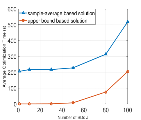
Figure 3: Average optimization time versus number of BDs J𝐽J.

Refer to caption

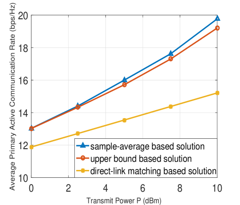
Figure 4: Average primary active communication rate versus transmit power.

Refer to caption

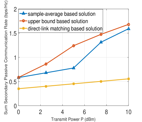
Figure 5: Secondary passive communication rate versus transmit power.

Fig. 3 plots the average optimization time versus the number of BDs for the two proposed solutions, where the average is taken over 100 independent channel realizations and S=1000𝑆1000S=1000 independent samples. The transmit power is P=0𝑃0P=0 dBm. It is observed that the optimization time increases monotonically with the number of BDs J𝐽J, which is expected since the matrix dimension of the constraint term in (50) becomes larger as J𝐽J increases. It can also be observed that the average optimization time of the upper bound based solution is much lower than that of the sample-average based solution.

Fig. 4 and Fig. 5 compare the performance of the average rate of primary active communication and secondary passive communication with three different precoding schemes, where the average is taken over S=1000𝑆1000S=1000 independent samples. Besides our proposed sample average based solution and the upper bound based solution in subsection V B, we also consider the direct-link matching precoding scheme as a benchmark, where the PT ignores the multipath created by the BDs and simply sets the precoding matrix to match the direct link, i.e., 𝐅=1M_t𝐕_𝐇_d𝐏12𝐅1subscript𝑀_𝑡subscript𝐕_subscript𝐇_𝑑superscript𝐏12{\mathbf{F}=\frac{1}{\sqrt{{{M}_{\_}{t}}}}{{\mathbf{V}}_{\_}{{\mathbf{H}_{\_}{d}}}}{{\mathbf{P}}^{\frac{1}{2}}}}, with 𝐕_𝐇_dsubscript𝐕_subscript𝐇_𝑑{{\mathbf{V}}_{\_}{{\mathbf{H}_{\_}{d}}}} obtained based on the (reduced) SVD of the channel matrix, 𝐇_d=𝐔_𝐇_d𝚺_𝐇_d𝐕_𝐇_dHsubscript𝐇_𝑑subscript𝐔_subscript𝐇_𝑑subscript𝚺_subscript𝐇_𝑑subscript𝐕_subscript𝐇_superscript𝑑H{{\mathbf{{H}}}_{\_}{d}}={{\mathbf{U}}_{\_}{{{{\mathbf{{H}}}}_{\_}{d}}}}{{\mathbf{\Sigma}}_{\_}{{{{\mathbf{{H}}}}_{\_}{d}}}}\mathbf{V}_{\_}{{{{\mathbf{{H}}}}_{\_}{d}}}^{\text{H}}. The results in Fig. 4 and Fig. 5 are obtained for one realization of the channels, and the number of BDs is J=50𝐽50J=50. It is observed that for all the three precoding schemes, the average primary active rate and secondary passive rate increase monotonically with the transmit power P𝑃P, as expected. Furthermore, both our proposed solutions in subsection V B significantly outperform the benchmarking direct-link matching precoding scheme, thanks to the consideration of the effective channel constituted by both the direct link and the backscattered multipaths. Furthermore, it is observed that the sample-average based solution achieves slightly higher primary rate than the upper bound based solution, but at the cost of higher computation complexity, as illustrated in Fig. 3.
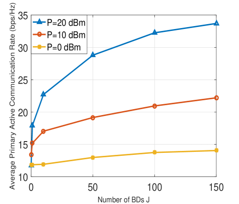
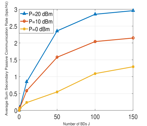
Refer to caption

Figure 6: Average primary communication rate versus number of BDs J𝐽J.

Refer to caption

Figure 7: Average secondary communication rate versus number of BDs J𝐽J.

Next, we study the impact of the number of BDs J𝐽J on the average primary and secondary communication rates, where the average is taken over 100 independent channel realizations and S𝑆S independent samples. For each channel realization, the primary communication rate is obtained with the proposed upper bound based solution. Note that though sub-optimal in general, the upper bound based solution has much lower computational complexity than the sample-average based solution. Fig. 6 and Fig. 7 plot the average primary and secondary communication rates versus the number of BDs J𝐽J, respectively. It is firstly observed that the primary communication rate is in general much higher than the secondary rate. This is expected since the symbol rate of primary signals is K=128𝐾128K=128 times of that of the secondary signals, and that the backscattered link for one single BD is in general much weaker than the primary communication link. Furthermore, it is observed that as J𝐽J increases, both primary and secondary rates increase, which corroborates our theoretical results in Section III.

VII Conclusion

In this paper, a MIMO symbiotic radio system with a massive number of BDs was investigated. The achievable rates of both the primary active communication and secondary passive communication were derived. Furthermore, considering the asymptotic regime as the number of BDs goes large, closed-form expressions were derived for the general MIMO symbiotic radio setup and the special SIMO setup, both of which were shown to be increasing functions of the number of BDs. This thus demonstrated that the mutualism relationship of symbiotic radio can be fully exploited with massive BD access. In addition, the precoding optimization problem was studied to maximize the primary communication rate while guaranteeing that the secondary communication rate was no smaller than a certain threshold. Extensive simulation results were provided to verify the effectiveness of our proposed solutions.

Appendix A Proof of Theorem 1

Denote the right hand side of (13) in Theorem 1 as C𝐶C, which can be expressed as

C=1Klog_2|𝐈_M_rM_s+1σ2_j=1J𝐱_j𝐱_jH|=1Klog_2|𝐈_M_rM_s+1σ2_j=2J𝐱_j𝐱_jH+1σ2𝐱_1𝐱_1H|.\begin{split}C&=\frac{1}{K}{{\log}_{\_}{2}}\Big{|}{{\mathbf{I}}_{\_}{M_{\_}rM_{\_}s}}+\frac{1}{{{\sigma}^{2}}}\sum\limits_{\_}{j=1}^{J}{{{\mathbf{x}}_{\_}{j}}\mathbf{x}_{\_}{j}^{\text{H}}}\Big{|}\\ &=\frac{1}{K}{{\log}_{\_}{2}}\Big{|}{{\mathbf{I}}_{\_}{M_{\_}rM_{\_}s}}+\frac{1}{{{\sigma}^{2}}}\sum\limits_{\_}{j=2}^{J}{{{\mathbf{x}}_{\_}{j}}\mathbf{x}_{\_}{j}^{\text{H}}+\frac{1}{{{\sigma}^{2}}}{{\mathbf{x}}_{\_}{1}}\mathbf{x}_{\_}{1}^{\text{H}}}\Big{|}.\\ \end{split} (60)

Let 𝐀_i=𝐈_M_rM_s+1σ2_j=i+1J𝐱_j𝐱_jHsubscript𝐀_𝑖subscript𝐈_subscript𝑀_𝑟subscript𝑀_𝑠1superscript𝜎2subscript_𝑗𝑖superscript1𝐽subscript𝐱_𝑗subscript𝐱_superscript𝑗H{{\mathbf{A}}_{\_}{i}}={{\mathbf{I}}_{\_}{M_{\_}rM_{\_}s}}+\frac{1}{{{\sigma}^{2}}}\sum\limits_{\_}{j=i+1}^{J}{{{\mathbf{x}}_{\_}{j}}\mathbf{x}_{\_}{j}^{\text{H}}}, then C𝐶C can be expressed as

C=1Klog_2|𝐀_0|=1Klog_2|𝐀_1+1σ2𝐱_1𝐱_1H|=1Klog_2|𝐀_1(𝐈_M_rM_s+1σ2𝐀_11𝐱_1𝐱_1H)|=1Klog_2|𝐀_1|+1Klog_2|𝐈_M_rM_s+1σ2𝐀_11𝐱_1𝐱_1H|=1Klog_2|𝐀_1|+1Klog_2(1+1σ2𝐱_1H𝐀_11𝐱_1)=1Klog_2|𝐀_1|+1Klog_2(1+γ_c_1),𝐶1𝐾subscript_2subscript𝐀_01𝐾subscript_2subscript𝐀_11superscript𝜎2subscript𝐱_1subscript𝐱_superscript1H1𝐾subscript_2subscript𝐀_1subscript𝐈_subscript𝑀_𝑟subscript𝑀_𝑠1superscript𝜎2subscript𝐀_superscript11subscript𝐱_1subscript𝐱_superscript1H1𝐾subscript_2subscript𝐀_11𝐾subscript_2subscript𝐈_subscript𝑀_𝑟subscript𝑀_𝑠1superscript𝜎2subscript𝐀_superscript11subscript𝐱_1subscript𝐱_superscript1H1𝐾subscript_2subscript𝐀_11𝐾subscript_211superscript𝜎2subscript𝐱_superscript1Hsubscript𝐀_superscript11subscript𝐱_11𝐾subscript_2subscript𝐀_11𝐾subscript_21subscript𝛾_subscript𝑐_1\begin{split}C&=\frac{1}{K}{{\log}_{\_}{2}}\left|{{\mathbf{A}}_{\_}{0}}\right|=\frac{1}{K}{{\log}_{\_}{2}}\Big{|}{{\mathbf{A}}_{\_}{1}}+\frac{1}{{{\sigma}^{2}}}{{\mathbf{x}}_{\_}{1}}\mathbf{x}_{\_}{1}^{\text{H}}\Big{|}\\ &=\frac{1}{K}{{\log}_{\_}{2}}\Big{|}{{\mathbf{A}}_{\_}{1}}\Big{(}{{\mathbf{I}}_{\_}{M_{\_}rM_{\_}s}}+\frac{1}{{{\sigma}^{2}}}\mathbf{A}_{\_}{1}^{-1}{{\mathbf{x}}_{\_}{1}}\mathbf{x}_{\_}{1}^{\text{H}}\Big{)}\Big{|}\\ &=\frac{1}{K}{{\log}_{\_}{2}}\left|{{\mathbf{A}}_{\_}{1}}\right|+\frac{1}{K}{{\log}_{\_}{2}}\Big{|}{{\mathbf{I}}_{\_}{M_{\_}rM_{\_}s}}+\frac{1}{{{\sigma}^{2}}}\mathbf{A}_{\_}{1}^{-1}{{\mathbf{x}}_{\_}{1}}\mathbf{x}_{\_}{1}^{\text{H}}\Big{|}\\ &=\frac{1}{K}{{\log}_{\_}{2}}\left|{{\mathbf{A}}_{\_}{1}}\right|+\frac{1}{K}{{\log}_{\_}{2}}\Big{(}1+\frac{1}{{{\sigma}^{2}}}\mathbf{x}_{\_}{1}^{\text{H}}\mathbf{A}_{\_}{1}^{-1}{{\mathbf{x}}_{\_}{1}}\Big{)}\\ &=\frac{1}{K}{{\log}_{\_}{2}}\left|{{\mathbf{A}}_{\_}{1}}\right|+\frac{1}{K}{{\log}_{\_}{2}}\left(1+{{\gamma}_{\_}{{{c}_{\_}{1}}}}\right),\\ \end{split} (61)

where the second last equality follows from the Weinstein-Aronszajn identity |𝐈_m+𝐀𝐁|=|𝐈_n+𝐁𝐀|subscript𝐈_𝑚𝐀𝐁subscript𝐈_𝑛𝐁𝐀\left|{{\mathbf{I}}_{\_}{m}}+\mathbf{AB}\right|=\left|{{\mathbf{I}}_{\_}{n}}+\mathbf{BA}\right|, and γ_c_1subscript𝛾_subscript𝑐_1{\gamma}_{\_}{{c}_{\_}{1}} is the maximum SINR of BD 1 given in (11). By applying the similar decomposition, 1Klog_2|𝐀_1|1𝐾subscript_2subscript𝐀_1\frac{1}{K}{{\log}_{\_}{2}}\left|{{\mathbf{A}}_{\_}{1}}\right| can be expressed as

1Klog_2|𝐀_1|=1Klog_2|𝐀_2|+1Klog_2(1+γ_c_2).1𝐾subscript_2subscript𝐀_11𝐾subscript_2subscript𝐀_21𝐾subscript_21subscript𝛾_subscript𝑐_2{\frac{1}{K}{{\log}_{\_}{2}}\left|{{\mathbf{A}}_{\_}{1}}\right|=\frac{1}{K}{{\log}_{\_}{2}}\left|{{\mathbf{A}}_{\_}{2}}\right|+\frac{1}{K}{{\log}_{\_}{2}}\left(1+{{\gamma}_{\_}{{{c}_{\_}{2}}}}\right)}. (62)

By applying the above result recursively, C𝐶C can be expressed as a general form

C=1Klog_2|𝐀_j|+1K_i=1jlog_2(1+γ_c_i).𝐶1𝐾subscript_2subscript𝐀_𝑗1𝐾subscript_𝑖superscript1𝑗subscript_21subscript𝛾_subscript𝑐_𝑖{C=\frac{1}{K}{{\log}_{\_}{2}}\left|{{\mathbf{A}}_{\_}{j}}\right|+\frac{1}{K}\sum\limits_{\_}{i=1}^{j}{{{\log}_{\_}{2}}\left(1+{{\gamma}_{\_}{{{c}_{\_}{i}}}}\right)}}. (63)

By letting j=J𝑗𝐽j=J, (63) can be expressed as

C=1Klog_2|𝐀_J|+1K_i=1Jlog_2(1+γ_c_i)=1K_j=1Jlog_2(1+γ_c_j)=R_BD.𝐶1𝐾subscript_2subscript𝐀_𝐽1𝐾subscript_𝑖superscript1𝐽subscript_21subscript𝛾_subscript𝑐_𝑖1𝐾subscript_𝑗superscript1𝐽subscript_21subscript𝛾_subscript𝑐_𝑗subscript𝑅_𝐵𝐷\begin{split}C&=\frac{1}{K}{{\log}_{\_}{2}}\left|{{\mathbf{A}}_{\_}{J}}\right|+\frac{1}{K}\sum\limits_{\_}{i=1}^{J}{{{\log}_{\_}{2}}\left(1+{{\gamma}_{\_}{{{c}_{\_}{i}}}}\right)}\\ &=\frac{1}{K}\sum\limits_{\_}{j=1}^{J}{{{\log}_{\_}{2}}\left(1+{{\gamma}_{\_}{{{c}_{\_}{j}}}}\right)}=R_{\_}{BD}.\\ \end{split} (64)

This thus completes the proof of Theorem 1.

Appendix B Proof of Lemma 1

To show Lemma 1, by substituting 𝐱_j=KPαvec(𝐠_j𝐡_jH𝐅)subscript𝐱_𝑗𝐾𝑃𝛼vecsubscript𝐠_𝑗subscript𝐡_superscript𝑗H𝐅{\mathbf{x}}_{\_}{j}=\sqrt{KP\alpha}\text{vec}\left({{\mathbf{g}}_{\_}{j}}\mathbf{h}_{\_}{j}^{\text{H}}\mathbf{F}\right), we have

𝐱_j𝐱_jH=KPαvec(𝐠_j1𝐡_jH𝐅)vec(𝐠_j1𝐡_jH𝐅)H=KPα((𝐡_jH𝐅)T𝐠_j)((𝐡_jH𝐅)T𝐠_j)H=KPα(𝐅T𝐡_j𝐡_jT𝐅)(𝐠_j𝐠_jH),subscript𝐱_𝑗subscript𝐱_superscript𝑗H𝐾𝑃𝛼vecsubscript𝐠_𝑗1subscript𝐡_superscript𝑗H𝐅vecsuperscriptsubscript𝐠_𝑗1subscript𝐡_superscript𝑗H𝐅H𝐾𝑃𝛼tensor-productsuperscriptsubscript𝐡_superscript𝑗H𝐅Tsubscript𝐠_𝑗superscripttensor-productsuperscriptsubscript𝐡_superscript𝑗H𝐅Tsubscript𝐠_𝑗Htensor-product𝐾𝑃𝛼superscript𝐅Tsubscript𝐡_superscript𝑗subscript𝐡_superscript𝑗Tsuperscript𝐅subscript𝐠_𝑗subscript𝐠_superscript𝑗H\begin{split}{{\mathbf{x}}_{\_}{j}}\mathbf{x}_{\_}{j}^{\text{H}}&=KP\alpha\text{vec}\left({{\mathbf{g}}_{\_}{j}}\cdot 1\cdot\mathbf{h}_{\_}{j}^{\text{H}}\mathbf{F}\right)\text{vec}{{\left({{\mathbf{g}}_{\_}{j}}\cdot 1\cdot\mathbf{h}_{\_}{j}^{\text{H}}\mathbf{F}\right)}^{\text{H}}}\\ &=KP\alpha\left({{\left(\mathbf{h}_{\_}{j}^{\text{H}}\mathbf{F}\right)}^{\text{T}}}\otimes{{\mathbf{g}}_{\_}{j}}\right){{\left({{\left(\mathbf{h}_{\_}{j}^{\text{H}}\mathbf{F}\right)}^{\text{T}}}\otimes{{\mathbf{g}}_{\_}{j}}\right)}^{\text{H}}}\\ &=KP\alpha\left({{\mathbf{F}}^{\text{T}}}\mathbf{h}_{\_}{j}^{*}\mathbf{h}_{\_}{j}^{\text{T}}{{\mathbf{F}}^{*}}\right)\otimes\left({{\mathbf{g}}_{\_}{j}}\mathbf{g}_{\_}{j}^{\text{H}}\right),\end{split} (65)

where the second equality follows from the identity vec(𝐀_1𝐀_2𝐀_3)=(𝐀_3T𝐀_1)vec(𝐀_2)vecsubscript𝐀_1subscript𝐀_2subscript𝐀_3tensor-productsubscript𝐀_superscript3Tsubscript𝐀_1vecsubscript𝐀_2\text{vec}({{\mathbf{A}}_{\_}{1}}{{\mathbf{A}}_{\_}{2}}{{\mathbf{A}}_{\_}{3}})=\left(\mathbf{A}_{\_}{3}^{\text{T}}\otimes{{\mathbf{A}}_{\_}{1}}\right)\text{vec}({{\mathbf{A}}_{\_}{2}}), and the last equality follows from (𝐀𝐁)H=𝐀H𝐁Hsuperscripttensor-product𝐀𝐁Htensor-productsuperscript𝐀Hsuperscript𝐁H{{\left(\mathbf{A}\otimes\mathbf{B}\right)}^{\text{H}}}={{\mathbf{A}}^{\text{H}}}\otimes{{\mathbf{B}}^{\text{H}}} and (𝐀𝐁)(𝐂𝐃)=𝐀𝐂𝐁𝐃tensor-product𝐀𝐁tensor-product𝐂𝐃tensor-product𝐀𝐂𝐁𝐃\left(\mathbf{A}\otimes\mathbf{B}\right)\left(\mathbf{C}\otimes\mathbf{D}\right)=\mathbf{AC}\otimes\mathbf{BD}. Thus, R_BDsubscript𝑅_𝐵𝐷{{R}_{\_}{BD}} in (13) can be expressed as

R_BD=1Klog_2|𝐈_M_rM_s+1σ2_j=1J𝐱_j𝐱_jH|=1Klog_2|𝐈_M_rM_s+KP¯α_j=1J((𝐅T𝐡_j𝐡_jT𝐅)𝐠_j𝐠_jH)|=1Klog_2|(𝐈_M_rM_s+KP¯α_j=1J((𝐅T𝐡_j𝐡_jT𝐅)𝐠_j𝐠_jH))T|=1Klog_2|𝐈_M_rM_s+KP¯α_j=1J((𝐅H𝐡_j𝐡_jH𝐅)(𝐠_j𝐠_jH)T)|.\begin{split}{{R}_{\_}{BD}}&=\frac{1}{K}{{\log}_{\_}{2}}\Big{|}{{\mathbf{I}}_{\_}{M_{\_}rM_{\_}s}}+\frac{1}{{{\sigma}^{2}}}\sum\limits_{\_}{j=1}^{J}{{{\mathbf{x}}_{\_}{j}}\mathbf{x}_{\_}{j}^{\text{H}}}\Big{|}\\ &=\frac{1}{K}{{\log}_{\_}{2}}\Big{|}{{\mathbf{I}}_{\_}{M_{\_}rM_{\_}s}}+{K\bar{P}\alpha}\sum\limits_{\_}{j=1}^{J}{\left(\left({{\mathbf{F}}^{\text{T}}}\mathbf{h}_{\_}{j}^{*}\mathbf{h}_{\_}{j}^{\text{T}}{{\mathbf{F}}^{*}}\right)\otimes{{\mathbf{g}}_{\_}{j}}\mathbf{g}_{\_}{j}^{\text{H}}\right)}\Big{|}\\ &=\frac{1}{K}{{\log}_{\_}{2}}\Big{|}{{\Big{(}{{\mathbf{I}}_{\_}{M_{\_}rM_{\_}s}}+{K\bar{P}\alpha}\sum\limits_{\_}{j=1}^{J}{\left(\left({{\mathbf{F}}^{\text{T}}}\mathbf{h}_{\_}{j}^{*}\mathbf{h}_{\_}{j}^{\text{T}}{{\mathbf{F}}^{*}}\right)\otimes{{\mathbf{g}}_{\_}{j}}\mathbf{g}_{\_}{j}^{\text{H}}\right)}\Big{)}}^{\text{T}}}\Big{|}\\ &=\frac{1}{K}{{\log}_{\_}{2}}\Big{|}{{\mathbf{I}}_{\_}{M_{\_}rM_{\_}s}}+{K\bar{P}\alpha}\sum\limits_{\_}{j=1}^{J}{\left(\left({{\mathbf{F}}^{\text{H}}}{{\mathbf{h}}_{\_}{j}}\mathbf{h}_{\_}{j}^{\text{H}}\mathbf{F}\right)\otimes{{\left({{\mathbf{g}}_{\_}{j}}\mathbf{g}_{\_}{j}^{\text{H}}\right)}^{\text{T}}}\right)}\Big{|}.\end{split} (66)

This thus completes the proof of Lemma 1.

Appendix C Proof of Lemma 2

By using the law of large numbers, for J1much-greater-than𝐽1J\gg 1, we have:

_j=1J((𝐅H𝐡_j𝐡_jH𝐅)(𝐠_j𝐠_jH)T)J𝔼[(𝐅H𝐡_j𝐡_jH𝐅)(𝐠_j𝐠_jH)T]=J𝔼[(𝐅H𝐡_j𝐡_jH𝐅)]𝔼[(𝐠_j𝐠_jH)T]=Jβ_hβ_g(𝐅H𝐅)𝐈_M_r.subscript_𝑗superscript1𝐽tensor-productsuperscript𝐅Hsubscript𝐡_𝑗subscript𝐡_superscript𝑗H𝐅superscriptsubscript𝐠_𝑗subscript𝐠_superscript𝑗HT𝐽𝔼delimited-[]tensor-productsuperscript𝐅Hsubscript𝐡_𝑗subscript𝐡_superscript𝑗H𝐅superscriptsubscript𝐠_𝑗subscript𝐠_superscript𝑗HTtensor-product𝐽𝔼delimited-[]superscript𝐅Hsubscript𝐡_𝑗subscript𝐡_superscript𝑗H𝐅𝔼delimited-[]superscriptsubscript𝐠_𝑗subscript𝐠_superscript𝑗HTtensor-product𝐽subscript𝛽_subscript𝛽_𝑔superscript𝐅H𝐅subscript𝐈_subscript𝑀_𝑟\begin{split}&\sum\limits_{\_}{j=1}^{J}{\left(\left({{\mathbf{F}}^{\text{H}}}{{\mathbf{h}}_{\_}{j}}\mathbf{h}_{\_}{j}^{\text{H}}\mathbf{F}\right)\otimes{{\left({{\mathbf{g}}_{\_}{j}}\mathbf{g}_{\_}{j}^{\text{H}}\right)}^{\text{T}}}\right)}\\ &\to J\mathbb{E}\left[\left({{\mathbf{F}}^{\text{H}}}{{\mathbf{h}}_{\_}{j}}\mathbf{h}_{\_}{j}^{\text{H}}\mathbf{F}\right)\otimes{{\left({{\mathbf{g}}_{\_}{j}}\mathbf{g}_{\_}{j}^{\text{H}}\right)}^{\text{T}}}\right]\\ &=J\mathbb{E}\left[\left({{\mathbf{F}}^{\text{H}}}{{\mathbf{h}}_{\_}{j}}\mathbf{h}_{\_}{j}^{\text{H}}\mathbf{F}\right)\right]\otimes\mathbb{E}\left[{{\left({{\mathbf{g}}_{\_}{j}}\mathbf{g}_{\_}{j}^{\text{H}}\right)}^{\text{T}}}\right]\\ &=J{{\beta}_{\_}{h}}{{\beta}_{\_}{g}}\left({{\mathbf{F}}^{\text{H}}}\mathbf{F}\right)\otimes{{\mathbf{I}}_{\_}{M_{\_}r}}.\end{split} (67)

It then follows from (14) that

R_BD1Klog_2|𝐈_M_rM_s+JKP¯αβ_hβ_g(𝐅H𝐅𝐈_M_r)|=1Klog_2|(𝐈_M_s+JKP¯αβ_hβ_g𝐅H𝐅)𝐈_M_r|=1Klog_2(|𝐈_M_s+JKP¯αβ_hβ_g𝐅H𝐅|M_r|𝐈_M_r|M_s)=M_rKlog_2|𝐈_M_s+JKP¯αβ_hβ_g𝐅H𝐅|=M_rKlog_2|𝐈_M_t+JKP¯αβ_hβ_g𝐅𝐅H|,subscript𝑅_𝐵𝐷1𝐾subscript_2subscript𝐈_subscript𝑀_𝑟subscript𝑀_𝑠𝐽𝐾¯𝑃𝛼subscript𝛽_subscript𝛽_𝑔tensor-productsuperscript𝐅H𝐅subscript𝐈_subscript𝑀_𝑟1𝐾subscript_2tensor-productsubscript𝐈_subscript𝑀_𝑠𝐽𝐾¯𝑃𝛼subscript𝛽_subscript𝛽_𝑔superscript𝐅H𝐅subscript𝐈_subscript𝑀_𝑟1𝐾subscript_2superscriptsubscript𝐈_subscript𝑀_𝑠𝐽𝐾¯𝑃𝛼subscript𝛽_subscript𝛽_𝑔superscript𝐅H𝐅subscript𝑀_𝑟superscriptsubscript𝐈_subscript𝑀_𝑟subscript𝑀_𝑠subscript𝑀_𝑟𝐾subscript_2subscript𝐈_subscript𝑀_𝑠𝐽𝐾¯𝑃𝛼subscript𝛽_subscript𝛽_𝑔superscript𝐅H𝐅subscript𝑀_𝑟𝐾subscript_2subscript𝐈_subscript𝑀_𝑡𝐽𝐾¯𝑃𝛼subscript𝛽_subscript𝛽_𝑔superscript𝐅𝐅H\begin{split}{{R}_{\_}{BD}}&\to\frac{1}{K}{{\log}_{\_}{2}}\left|{{\mathbf{I}}_{\_}{M_{\_}rM_{\_}s}}+{JK\bar{P}\alpha{{\beta}_{\_}{h}}{{\beta}_{\_}{g}}}\left({{\mathbf{F}}^{\text{H}}}\mathbf{F}\otimes{{\mathbf{I}}_{\_}{M_{\_}r}}\right)\right|\\ &=\frac{1}{K}{{\log}_{\_}{2}}\left|\left({{\mathbf{I}}_{\_}{M_{\_}s}}+{JK\bar{P}\alpha{{\beta}_{\_}{h}}{{\beta}_{\_}{g}}}{{\mathbf{F}}^{\text{H}}}\mathbf{F}\right)\otimes{{\mathbf{I}}_{\_}{M_{\_}r}}\right|\\ &=\frac{1}{K}{{\log}_{\_}{2}}\left({{\left|{{\mathbf{I}}_{\_}{M_{\_}s}}+{JK\bar{P}\alpha{{\beta}_{\_}{h}}{{\beta}_{\_}{g}}}{{\mathbf{F}}^{\text{H}}}\mathbf{F}\right|}^{M_{\_}r}}{{\left|{{\mathbf{I}}_{\_}{M_{\_}r}}\right|}^{M_{\_}s}}\right)\\ &=\frac{M_{\_}r}{K}{{\log}_{\_}{2}}\left|{{\mathbf{I}}_{\_}{M_{\_}s}}+{JK\bar{P}\alpha{{\beta}_{\_}{h}}{{\beta}_{\_}{g}}}{{\mathbf{F}}^{\text{H}}}\mathbf{F}\right|\\ &=\frac{M_{\_}r}{K}{{\log}_{\_}{2}}\left|{{\mathbf{I}}_{\_}{M_{\_}t}}+{JK\bar{P}\alpha{{\beta}_{\_}{h}}{{\beta}_{\_}{g}}}\mathbf{F}{{\mathbf{F}}^{\text{H}}}\right|,\end{split} (68)

where the third last equality follows from the identity |𝐀𝐁|=|𝐀|rank(𝐁)|𝐁|rank(𝐀)tensor-product𝐀𝐁superscript𝐀rank𝐁superscript𝐁rank𝐀\left|\mathbf{A}\otimes\mathbf{B}\right|={{\left|\mathbf{A}\right|}^{\text{rank}(\mathbf{B})}}{{\left|\mathbf{B}\right|}^{\text{rank}(\mathbf{A})}}.

This completes the proof of Lemma 2.

Appendix D Proof of Lemma 3

According to (3), we have

R_s=𝔼_𝐜(n)[log_2|𝐈_M_r+P¯𝐇_eq(𝐜(n))𝐅𝐅H𝐇_eqH(𝐜(n))|]=𝔼_𝐜(n)[log_2|𝐈_M_t+P¯𝐅𝐅H𝐇_eqH(𝐜(n))𝐇_eq(𝐜(n))|].subscript𝑅_𝑠subscript𝔼_𝐜𝑛delimited-[]subscript_2subscript𝐈_subscript𝑀_𝑟¯𝑃subscript𝐇_𝑒𝑞𝐜𝑛superscript𝐅𝐅Hsubscript𝐇_𝑒superscript𝑞H𝐜𝑛subscript𝔼_𝐜𝑛delimited-[]subscript_2subscript𝐈_subscript𝑀_𝑡¯𝑃superscript𝐅𝐅Hsubscript𝐇_𝑒superscript𝑞H𝐜𝑛subscript𝐇_𝑒𝑞𝐜𝑛\begin{split}{{R}_{\_}{s}}&={{\mathbb{E}}_{\_}{\mathbf{c}(n)}}\left[{{\log}_{\_}{2}}\left|{{\mathbf{I}}_{\_}{{{M}_{\_}{r}}}}+{\bar{P}}{{\mathbf{H}}_{\_}{eq}}\left(\mathbf{c}\left(n\right)\right)\mathbf{F}{{\mathbf{F}}^{\text{H}}}\mathbf{H}_{\_}{eq}^{\text{H}}\left(\mathbf{c}\left(n\right)\right)\right|\right]\\ &={{\mathbb{E}}_{\_}{\mathbf{c}(n)}}\left[{{\log}_{\_}{2}}\left|{{\mathbf{I}}_{\_}{{{M}_{\_}{t}}}}+{\bar{P}}\mathbf{F}{{\mathbf{F}}^{\text{H}}}\mathbf{H}_{\_}{eq}^{\text{H}}\left(\mathbf{c}\left(n\right)\right){{\mathbf{H}}_{\_}{eq}}\left(\mathbf{c}\left(n\right)\right)\right|\right].\\ \end{split} (69)

Furthermore, we have

𝐇_eqH(𝐜(n))𝐇_eq(𝐜(n))=(𝐇_d+_j=1Jα𝐠_j𝐡_jHc_j(n))H(𝐇_d+_j=1Jα𝐠_j𝐡_jHc_j(n))=𝐇_dH𝐇_d+α_j=1Jc_j(n)𝐡_j𝐠_jH𝐇_d+α_j=1Jc_j(n)𝐇_dH𝐠_j𝐡_jH+α_j=1J_i=1Jc_j(n)c_i(n)𝐡_j𝐠_jH𝐠_i𝐡_iH=𝐇_dH𝐇_d+α_j=1Jc_j(n)𝐡_j𝐠_jH𝐇_d+α_j=1Jc_j(n)𝐇_dH𝐠_j𝐡_jH+α_j=1J|c_j(n)|2𝐠_j2𝐡_j𝐡_jH+α_j=1,jiJ_i=1Jc_j(n)c_i(n)𝐡_j𝐠_jH𝐠_i𝐡_iH.formulae-sequencesubscript𝐇_𝑒superscript𝑞H𝐜𝑛subscript𝐇_𝑒𝑞𝐜𝑛superscriptsubscript𝐇_𝑑subscript_𝑗superscript1𝐽𝛼subscript𝐠_𝑗subscript𝐡_superscript𝑗Hsubscript𝑐_𝑗𝑛Hsubscript𝐇_𝑑subscript_𝑗superscript1𝐽𝛼subscript𝐠_𝑗subscript𝐡_superscript𝑗Hsubscript𝑐_𝑗𝑛subscript𝐇_superscript𝑑Hsubscript𝐇_𝑑𝛼subscript_𝑗superscript1𝐽subscript𝑐_superscript𝑗𝑛subscript𝐡_𝑗subscript𝐠_superscript𝑗Hsubscript𝐇_𝑑𝛼subscript_𝑗superscript1𝐽subscript𝑐_𝑗𝑛subscript𝐇_superscript𝑑Hsubscript𝐠_𝑗subscript𝐡_superscript𝑗H𝛼subscript_𝑗superscript1𝐽subscript_𝑖superscript1𝐽subscript𝑐_superscript𝑗𝑛subscript𝑐_𝑖𝑛subscript𝐡_𝑗subscript𝐠_superscript𝑗Hsubscript𝐠_𝑖subscript𝐡_superscript𝑖Hsubscript𝐇_superscript𝑑Hsubscript𝐇_𝑑𝛼subscript_𝑗superscript1𝐽subscript𝑐_superscript𝑗𝑛subscript𝐡_𝑗subscript𝐠_superscript𝑗Hsubscript𝐇_𝑑𝛼subscript_𝑗superscript1𝐽subscript𝑐_𝑗𝑛subscript𝐇_superscript𝑑Hsubscript𝐠_𝑗subscript𝐡_superscript𝑗H𝛼subscript_𝑗superscript1𝐽superscriptsubscript𝑐_𝑗𝑛2superscriptdelimited-∥∥subscript𝐠_𝑗2subscript𝐡_𝑗subscript𝐡_superscript𝑗H𝛼subscript_𝑗1𝑗superscript𝑖𝐽subscript_𝑖superscript1𝐽subscript𝑐_superscript𝑗𝑛subscript𝑐_𝑖𝑛subscript𝐡_𝑗subscript𝐠_superscript𝑗Hsubscript𝐠_𝑖subscript𝐡_superscript𝑖H\begin{split}&\mathbf{H}_{\_}{eq}^{\text{H}}(\mathbf{c}(n)){{\mathbf{H}}_{\_}{eq}}(\mathbf{c}(n))\\ &={{\Big{(}{{\mathbf{H}}_{\_}{d}}+\sum\limits_{\_}{j=1}^{J}{\sqrt{\alpha}}{{\mathbf{g}}_{\_}{j}}\mathbf{h}_{\_}{j}^{\text{H}}{{c}_{\_}{j}}(n)\Big{)}}^{\text{H}}}\Big{(}{{\mathbf{H}}_{\_}{d}}+\sum\limits_{\_}{j=1}^{J}{\sqrt{\alpha}}{{\mathbf{g}}_{\_}{j}}\mathbf{h}_{\_}{j}^{\text{H}}{{c}_{\_}{j}}(n)\Big{)}\\ &=\mathbf{H}_{\_}{d}^{\text{H}}{{\mathbf{H}}_{\_}{d}}+\sqrt{\alpha}\sum\limits_{\_}{j=1}^{J}{c_{\_}{j}^{*}(n)}{{\mathbf{h}}_{\_}{j}}\mathbf{g}_{\_}{j}^{\text{H}}{{\mathbf{H}}_{\_}{d}}+\sqrt{\alpha}\sum\limits_{\_}{j=1}^{J}{{{c}_{\_}{j}}(n)\mathbf{H}_{\_}{d}^{\text{H}}}{{\mathbf{g}}_{\_}{j}}\mathbf{h}_{\_}{j}^{\text{H}}\\ &+\alpha\sum\limits_{\_}{j=1}^{J}{\sum\limits_{\_}{i=1}^{J}{c_{\_}{j}^{*}(n){{c}_{\_}{i}}(n)}}{{\mathbf{h}}_{\_}{j}}\mathbf{g}_{\_}{j}^{\text{H}}{{\mathbf{g}}_{\_}{i}}\mathbf{h}_{\_}{i}^{\text{H}}\\ &=\mathbf{H}_{\_}{d}^{\text{H}}{{\mathbf{H}}_{\_}{d}}+\sqrt{\alpha}\sum\limits_{\_}{j=1}^{J}{c_{\_}{j}^{*}(n)}{{\mathbf{h}}_{\_}{j}}\mathbf{g}_{\_}{j}^{\text{H}}{{\mathbf{H}}_{\_}{d}}+\sqrt{\alpha}\sum\limits_{\_}{j=1}^{J}{{{c}_{\_}{j}}(n)\mathbf{H}_{\_}{d}^{\text{H}}}{{\mathbf{g}}_{\_}{j}}\mathbf{h}_{\_}{j}^{\text{H}}\\ &+\alpha\sum\limits_{\_}{j=1}^{J}{{{\left|{{c}_{\_}{j}}(n)\right|}^{2}}}{{\left\|{{\mathbf{g}}_{\_}{j}}\right\|}^{2}}{{\mathbf{h}}_{\_}{j}}\mathbf{h}_{\_}{j}^{\text{H}}+\alpha\sum\limits_{\_}{j=1,j\neq i}^{J}{\sum\limits_{\_}{i=1}^{J}{c_{\_}{j}^{*}(n){{c}_{\_}{i}}(n)}}{{\mathbf{h}}_{\_}{j}}\mathbf{g}_{\_}{j}^{\text{H}}{{\mathbf{g}}_{\_}{i}}\mathbf{h}_{\_}{i}^{\text{H}}.\\ \end{split} (70)

Due to the law of large numbers, for J1much-greater-than𝐽1J\gg 1, we have: α_j=1,jiJ_i=1Jc_j(n)c_i(n)𝐡_j𝐠_jH𝐠_i𝐡_iH0formulae-sequence𝛼subscript_𝑗1𝑗superscript𝑖𝐽subscript_𝑖superscript1𝐽subscript𝑐_superscript𝑗𝑛subscript𝑐_𝑖𝑛subscript𝐡_𝑗subscript𝐠_superscript𝑗Hsubscript𝐠_𝑖subscript𝐡_superscript𝑖H0\alpha\sum\limits_{\_}{j=1,j\neq i}^{J}{\sum\limits_{\_}{i=1}^{J}{c_{\_}{j}^{*}(n){{c}_{\_}{i}}(n)}}{{\mathbf{h}}_{\_}{j}}\mathbf{g}_{\_}{j}^{\text{H}}{{\mathbf{g}}_{\_}{i}}\mathbf{h}_{\_}{i}^{\text{H}}\to 0. Therefore,

𝐇_eqH(𝐜(n))𝐇_eq(𝐜(n))𝐇_dH𝐇_d+Jα𝔼[c_j(n)𝐡_j𝐠_jH𝐇_d]+Jα𝔼[c_j(n)𝐇_dH𝐠_j𝐡_jH]+Jα𝔼[|c_j(n)|2𝐠_j2𝐡_j𝐡_jH]=𝐇_dH𝐇_d+JαM_rβ_gβ_h𝐈_M_t.subscript𝐇_𝑒superscript𝑞H𝐜𝑛subscript𝐇_𝑒𝑞𝐜𝑛subscript𝐇_superscript𝑑Hsubscript𝐇_𝑑𝐽𝛼𝔼delimited-[]subscript𝑐_superscript𝑗𝑛subscript𝐡_𝑗subscript𝐠_superscript𝑗Hsubscript𝐇_𝑑𝐽𝛼𝔼delimited-[]subscript𝑐_𝑗𝑛subscript𝐇_superscript𝑑Hsubscript𝐠_𝑗subscript𝐡_superscript𝑗H𝐽𝛼𝔼delimited-[]superscriptsubscript𝑐_𝑗𝑛2superscriptdelimited-∥∥subscript𝐠_𝑗2subscript𝐡_𝑗subscript𝐡_superscript𝑗Hsubscript𝐇_superscript𝑑Hsubscript𝐇_𝑑𝐽𝛼subscript𝑀_𝑟subscript𝛽_𝑔subscript𝛽_subscript𝐈_subscript𝑀_𝑡\begin{split}&\mathbf{H}_{\_}{eq}^{\text{H}}(\mathbf{c}(n)){{\mathbf{H}}_{\_}{eq}}(\mathbf{c}(n))\\ &\to\mathbf{H}_{\_}{d}^{\text{H}}{{\mathbf{H}}_{\_}{d}}+J\sqrt{\alpha}\mathbb{E}\left[c_{\_}{j}^{*}(n){{\mathbf{h}}_{\_}{j}}\mathbf{g}_{\_}{j}^{\text{H}}{{\mathbf{H}}_{\_}{d}}\right]+J\sqrt{\alpha}\mathbb{E}\left[{{c}_{\_}{j}}(n)\mathbf{H}_{\_}{d}^{\text{H}}{{\mathbf{g}}_{\_}{j}}\mathbf{h}_{\_}{j}^{\text{H}}\right]\\ &+J\alpha\mathbb{E}\left[{{\left|{{c}_{\_}{j}}(n)\right|}^{2}}{{\left\|{{\mathbf{g}}_{\_}{j}}\right\|}^{2}}{{\mathbf{h}}_{\_}{j}}\mathbf{h}_{\_}{j}^{\text{H}}\right]\\ &=\mathbf{H}_{\_}{d}^{\text{H}}{{\mathbf{H}}_{\_}{d}}+J\alpha{{M}_{\_}{r}}{{\beta}_{\_}{g}}{{\beta}_{\_}{h}}{{\mathbf{I}}_{\_}{{{M}_{\_}{t}}}}.\\ \end{split} (71)

By substituting (71) into (69), the proof of Lemma 3 thus completes.

References

  • [1] Y.-C. Liang, Q. Zhang, E. G. Larsson and G. Y. Li, “Symbiotic radio: Cognitive backscattering communications for future wireless networks,” IEEE Trans. Cognit. Commun. Netw., vol. 6, no. 4, pp. 1242–1255, Dec. 2020.
  • [2] G. Yang, Q. Zhang, and Y.-C. Liang, “Cooperative ambient backscatter communications for green Internet-of-Things,” IEEE Internet Things J., vol. 5, no. 2, pp. 1116–1130, Apr. 2018.
  • [3] H. Guo, Y.-C. Liang, R. Long, S. Xiao, and Q. Zhang, “Resource allocation for symbiotic radio system with fading channels,” IEEE Access, vol. 7, pp. 34333–34347, Mar. 2019.
  • [4] J. Mitola and G. Q. Maguire, “Cognitive radio: Making software radios more personal,” IEEE Pers. Commun., vol. 6, no. 4, pp. 13–18, Aug. 1999.
  • [5] S. Haykin, “Cognitive radio: Brain-empowered wireless communications,” IEEE J. Sel. Areas Commun., vol. 23, no. 2, pp. 201–220, Feb. 2005.
  • [6] B. Wang and K. J. R. Liu, “Advances in cognitive radio networks: A survey,” IEEE J. Sel. Topics Signal Process., vol. 5, no. 1, pp. 5–23, Feb. 2011.
  • [7] J. Xu, Z. Dai and Y. Zeng, “Enabling Full Mutualism for Symbiotic Radio with Massive Backscatter Devices,” in Proc. IEEE Glob. Commun. Conf.(GLOBECOM), 2021, pp. 1–6.
  • [8] V. Liu, A. Parks, V. Talla, S. Gollakota, D. Wetherall, and J. R. Smith, “Ambient backscatter: Wireless communication out of thin air,” in ACM SIGCOMM, Hong Kong, Jun. 2013, pp. 39–50.
  • [9] D. T. Hoang, D. Niyato, P. Wang, D. I. Kim, and Z. Han, “Ambient backscatter: A new approach to improve network performance for RF powered cognitive radio networks,” IEEE Trans. Commun., vol. 65, no. 9, pp. 3659–3674, Sep. 2017.
  • [10] N. Van Huynh, D. T. Hoang, X. Lu, D. Niyato, P. Wang, and D. I. Kim, “Ambient backscatter communications: A contemporary survey,” IEEE Commun. Surveys Tuts., vol. 20, no. 4, pp. 2889–2922, Fourth 2018.
  • [11] R. Long, Y.-C. Liang, H. Guo, G. Yang, and R. Zhang, “Symbiotic radio: A new communication paradigm for passive Internet-of-Things,” IEEE Internet Things J., vol. 7, pp. 1350–1363, Nov. 2020.
  • [12] S. J. Nawaz, S. K. Sharma, B. Mansoor, M. N. Patwary, and N. M. Khan, “Non-coherent and backscatter communications: Enabling ultra-massive connectivity in 6G wireless networks,” IEEE Access, vol. 9, pp. 38144–38186, Feb. 2021.
  • [13] L. Bariah, L. Mohjazi, S. Muhaidat, P. C. Sofotasios, G. K. Kurt, H. Yanikomeroglu, and O. A. Dobre, “A prospective look: key enabling technologies, applications and open research topics in 6G Networks,” IEEE Access, vol. 8, pp. 174792–174820, Aug. 2020.
  • [14] S. Chen, Y.-C. Liang, S. Sun, S. Kang, W. Cheng, and M. Peng, “Vision, requirements, and technology trend of 6G: how to tackle the challenges of system coverage, capacity, user data-rate and movement speed,” IEEE Wireless Commun., vol. 27, no. 2, pp. 218–228, Apr. 2020.
  • [15] Z. Chu, W. Hao, P. Xiao, M. Khalily and R. Tafazolli, “Resource allocations for symbiotic radio with finite blocklength backscatter link,” IEEE Internet Things J., vol. 7, no. 9, pp. 8192–8207, Sept. 2020.
  • [16] G. Yang, T. Wei and Y.-C. Liang, “Joint Hybrid and Passive Beamforming for Millimeter Wave Symbiotic Radio Systems,” IEEE Wireless Commun. Lett., vol. 10, no. 10, pp. 2294–2298, Oct. 2021.
  • [17] Y. Guo, G. Wang, R. Xu, R. He, X. Wei and C. Tellambura, “Capacity Analysis for Wireless Symbiotic Communication Systems With BPSK Tags Under Sensitivity Constraint,” IEEE Commun. Lett., vol. 26, no. 1, pp. 44–48, Jan. 2022.
  • [18] Q. Zhang, L. Zhang, Y.-C. Liang and P. Kam, “Backscatter-NOMA: A symbiotic system of cellular and Internet-of-Things networks,” IEEE Access, vol. 7, pp. 20000–20013, Feb. 2019.
  • [19] T. Wu, M. Jiang, Q. Zhang, Q. Li and J. Qin, “Beamforming design in multiple-input-multiple-output symbiotic radio backscatter systems,” IEEE Commun. Lett., doi: 10.1109/LCOMM.2021.3060468.
  • [20] Y. Liao, G. Yang and Y.-C. Liang, “Resource allocation in NOMA-enhanced full-duplex symbiotic radio networks,” IEEE Access, vol. 8, pp. 22709–22720, Jan. 2020.
  • [21] H. Yang, Y. Ye, K. Liang, and X. Chu, “Energy efficiency maximization for symbiotic radio networks with multiple backscatter devices,” IEEE open J. Commun. Soc., vol. 2, pp. 1431–1444, Jun. 2021.
  • [22] Z. Chu, W. Hao, P. Xiao, M. Khalily, and R. Tafazolli, “Resource allocations for symbiotic radio with finite blocklength backscatter link,” IEEE Internet Things J., vol. 7, no. 9, pp. 8192–8207, Sep. 2020.
  • [23] S. Wang, J. Xu, and Y. Zeng, “Characterizing the energy-efficiency region of symbiotic radio communications,” https://arxiv.org/abs/2205.03826.
  • [24] M. Elsayed, A. Samir, A. A. A. El-Banna, X. Li and B. M. ElHalawany,“When NOMA Multiplexing Meets Symbiotic Ambient Backscatter Communication: Outage Analysis,” IEEE Trans. Veh. Technol., vol.  71, no. 1, pp. 1026–1031, Jan. 2022.
  • [25] R. Zhang, X. Kang and Y.-C. Liang, “Minimum Throughput Maximization for Peer-Assisted NOMA-Plus-TDMA Symbiotic Radio Networks,” IEEE Wireless Commun. Lett., vol. 10, no. 9, pp. 1847–1851, Sept. 2021.
  • [26] R. Long, H. Guo, L. Zhang and Y.-C. Liang, “Full-duplex backscatter communications in symbiotic radio systems,” IEEE Access, vol. 7, pp. 21597–21608, Feb. 2019.
  • [27] G. Yang, D. Yuan, Y.-C. Liang, R. Zhang, and V. C. M. Leung, “Optimal resource allocation in full-duplex ambient backscatter communication networks for wireless-powered IoT,” IEEE Internet Things J., vol. 6, no. 2, pp. 2612–2625, Apr. 2019.
  • [28] Z. Dai, R. Li, J. Xu, Y. Zeng, and S. Jin, “Cell-free symbiotic radio: Channel estimation method and achievable rate analysis,” in Proc. IEEE/CIC Int. Conf. Commun. China (ICCC) Workshops, 2021, pp. 25–30.
  • [29] F. Amato, C. W. Peterson, B. P. Degnan, and G. D. Durgin, “Tunneling RFID tags for long-range and low-power microwave applications,” IEEE J. Radio Freq. Identif., vol. 2, no. 2, pp. 93–103, Jun. 2018.
  • [30] S. Khaledian, F. Farzami, H. Soury, B. Smida, and D. Erricolo, “Active two-way backscatter modulation: An analytical study,” IEEE Trans. Wireless Commun., vol. 18, no. 3, pp. 1874–1886, Mar. 2019.
  • [31] R. Long, Y.-C. Liang, Y. Pei and E. G. Larsson, “Active-Load Assisted Symbiotic Radio System in Cognitive Radio Network,” in IEEE Workshop Signal Process. Adv. Wireless Commun. (SPAWC), 2020, pp. 1–5.
  • [32] X. Lei, M. Wu, F. Zhou, X. Tang, R. Q. Hu and P. Fan, “Reconfigurable Intelligent Surface-Based Symbiotic Radio for 6G: Design, Challenges, and Opportunities,” IEEE Wireless Commun., vol. 28, no. 5, pp.210–216, Oct. 2021.
  • [33] M. Wu, X. Lei, X. Zhou, Y. Xiao, X. Tang and R. Q. Hu, “Reconfigurable Intelligent Surface Assisted Spatial Modulation for Symbiotic Radio,” IEEE Trans. Veh. Technol., vol. 70, no. 12, pp. 12918–12931, Dec. 2021.
  • [34] Q. Zhang, Y.-C. Liang and H. V. Poor, “Reconfigurable Intelligent Surface Assisted MIMO Symbiotic Radio Networks,” IEEE Trans. Commun., vol. 69, no. 7, pp. 4832–4846, Jul. 2021.
  • [35] Z. Zhang et al., “6G Wireless Networks: Vision, Requirements, Architecture, and Key Technologies,” IEEE Veh. Technol. Mag., vol. 14, no. 3, pp. 28–41, Sept. 2019.
  • [36] D. Tse and P. Viswanath, Fundamentals of Wireless Communication. Cambridge university press, 2005.
  • [37] B. Hassibi and B. M. Hochwald,“How much training is needed in multiple-antenna wireless links?,” IEEE Trans. Info. Theory, vol. 49, no. 4, pp. 951–963, Apr. 2003.
  • [38] Heath Jr, Robert W., and Angel Lozano, Foundations of MIMO communication. Cambridge University Press, 2018.
  • [39] M. Grant and S. Boyd, “CVX: Matlab software for disciplined convex programming.” [Online]. Available: cvxr.com/cvx.