Aligning individual brains
with Fused Unbalanced Gromov-Wasserstein

Abstract

Individual brains vary in both anatomy and functional organization, even within a given species. Inter-individual variability is a major impediment when trying to draw generalizable conclusions from neuroimaging data collected on groups of subjects. Current co-registration procedures rely on limited data, and thus lead to very coarse inter-subject alignments. In this work, we present a novel method for inter-subject alignment based on Optimal Transport, denoted as Fused Unbalanced Gromov Wasserstein (FUGW). The method aligns cortical surfaces based on the similarity of their functional signatures in response to a variety of stimulation settings, while penalizing large deformations of individual topographic organization. We demonstrate that FUGW is well-suited for whole-brain landmark-free alignment. The unbalanced feature allows to deal with the fact that functional areas vary in size across subjects. Our results show that FUGW alignment significantly increases between-subject correlation of activity for independent functional data, and leads to more precise mapping at the group level.

1 Introduction

The availability of millimeter or sub-millimeter anatomical or functional brain images has opened new horizons to neuroscience, namely that of mapping cognition in the human brain and detecting markers of diseases. Yet this endeavour has stumbled on the roadblock of inter-individual variability: while the overall organization of the human brain is largely invariant, two different brains (even from monozygotic twins [33]) may differ at the scale of centimeters in shape, folding pattern, and functional responses. The problem is further complicated by the fact that functional images are noisy, due to imaging limitations and behavioral differences across individuals that cannot be easily overcome. The status quo of the field is thus to rely on anatomy-based inter-individual alignment that approximately matches the outline of the brain [4] as well as its large-scale cortical folding patterns [12, 15]. Existing algorithms thus coarsely match anatomical features with diffeomorphic transformations, by warping individual data to a simplified template brain. Such methods lose much of the original individual detail and blur the functional information that can be measured in brain regions (see Figure 1).

Figure 1: High variability in human anatomies and functional MRI responses across subjects In this experiment contrasting areas of the brain which respond to mathematical tasks against other that don’t, we observe great variability in locations and strength of brain activations across subjects (row 1). The classical approach consists in wrapping this data to a common surface template (row 2), where they can be averaged, often resulting in loss of individual details and detection power. These images were generated using Nilearn software [1].

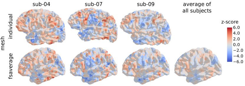
In order to improve upon the current situation, a number of challenges have to be addressed: (i) There exists no template brain with functional information, which by construction renders any cortical matching method blind to function. This is unfortunate, since functional information is arguably the most accessible marker to identify cortical regions and their boundaries [18]. (ii) When comparing two brains – coming from individuals or from a template – it is unclear what regularity should be imposed on the matching [42]. While it is traditional in medical imaging to impose diffeomorphicity [4], such a constrain does not match the frequent observation that brain regions vary across individuals in their fine-grained functional organization [18, 38]. (iii) Beyond the problem of aligning human brains, it is an even greater challenge to systematically compare functional brain organization in two different species, such as humans and macaques [26, 23, 46, 14]. Such inter-species comparisons introduce a more extreme form of variability in the correspondence model.

Related work

Several attempts have been made to constrain the brain alignment process by using functional information. The first one consists in introducing functional maps into the diffeomorphic framework and search for a smooth transformation that matches functional information [37, 47, 35], the most popular framework being arguably Multimodal Surface Matching (MSM) [35, 18].

A second family of less constrained functional alignment approaches have been proposed, based on heuristics, by matching information in small, possibly overlapping, cortical patches [21, 40, 6]. This popular framework has been called hyperalignment [21, 20], or shared response models [10]. Yet these approaches lack a principled framework and cannot be considered to solve the matching problem at scale. Neither do they allow to estimate a group-level template properly [45].

An alternative functional alignment framework has followed another path [19], considering functional signal as a three-dimensional distribution, and minimizing the transport cost. However, this framework imposes unnatural constraints of non-negativity of the signal and only works for one-dimensional contrasts, so that it cannot be used to learn multi-dimensional anatomo-functional structures. An important limitation of the latter two families of methods is that they operate on a fixed spatial context (mesh or voxel grid), and thus cannot be used on heterogeneous meshes such as between two individual human anatomies or, worse, between a monkey brain and a human brain.

Contributions

Following [5], we use the Wasserstein distance between source and target functional signals – consisting of contrast maps acquired with fMRI – to compute brain alignments. We contribute two notable extensions of this framework: (i) a Gromov-Wasserstein (GW) term to preserve global anatomical structure – this term introduces an anatomical penalization against improbably distant anatomical matches, yet without imposing diffeomorphic regularity – as well as (ii) an unbalanced correspondence that allows mappings from one brain to another to be incomplete, for instance because some functional areas are larger in some individuals than in others, or may simply be absent. We show that this approach successfully addresses the challenging case of different cortical meshes, and that derived brain activity templates are sharper than those obtained with standard anatomical alignment approaches.

2 Methods

Optimal Transport yields a natural framework to address the alignment problem, as it seeks to derive a plan – a coupling – that can be seen as a soft assignment matrix between cortical areas of a source and target individual. As discussed previously, there is a need for a functional alignment method that respects the rich geometric structure of the anatomical features, hence the Wasserstein distance alone is not sufficient. By construction, the GW distance [24, 25] can help preserve the global geometry underlying the signal. The more recent fused GW distance [44] goes one step further by making it possible to integrate functional data simultaneously with anatomical information.

2.1 Fused Unbalanced Gromov-Wasserstein

We leverage [44, 39] to present a new objective function which interpolates between a loss preserving the global geometry of the underlying mesh structure and a loss aligning source and target features, while simultaneously allowing not to transport some parts of the source and target distributions. We provide an open-source solver that minimizes this loss.

Formulation

We denote $\bm{F^{s}}\in\mathbb{R}^{n,c}$ the matrix of features per vertex for the source subject. In the proposed application, they correspond to $c$ functional activation maps, sampled on a mesh with $n$ vertices representing the source subject’s cortical surface. Let $\bm{D^{s}}\in\mathbb{R}^{n,n}_{+}$ be the matrix of pairwise geodesic distances between vertices of the source mesh. Moreover, we assign the distribution ${\bm{w^{s}}}\in\mathbb{R}^{n}_{+}$ on the source vertices. Comparably, we define $\bm{F^{t}}\in\mathbb{R}^{p,c}$, $\bm{D^{t}}\in\mathbb{R}^{p,p}_{+}$ and ${\bm{w^{t}}}\in\mathbb{R}^{p}_{+}$ for the target subject, whose individual anatomy is represented by a mesh comprising $p$ vertices. Eventually, $\bm{w^{s}}$ and $\bm{w^{t}}$ set the transportable mass per vertex, which, without prior knowledge, we choose to be uniform for the source and target vertices respectively: ${\bm{w^{s}}}\triangleq(\frac{1}{n},...,\frac{1}{n})$, ${\bm{w^{t}}}\triangleq(\frac{1}{p},...,\frac{1}{p})$.

Given a tuple of hyper-parameters $\theta\triangleq(\rho,\alpha,\varepsilon)$, where $\rho,\varepsilon\in\mathbb{R}_{+}$ and $\alpha\in[0,1]$, for any coupling $\bm{P}\in\mathbb{R}^{n,p}$, we define the fused unbalanced Gromov-Wasserstein loss as

$$\begin{split}\text{L}_{\theta}(\bm{P})\enspace\triangleq\enspace&(1-\alpha)\enspace\mathchoice{\leavevmode\hbox to90.18pt{\vbox to19.3pt{\pgfpicture\makeatletter\hbox{\hskip 45.09233pt\lower-10.00012pt\hbox to0.0pt{\pgfsys@beginscope\pgfsys@invoke{ }\definecolor{pgfstrokecolor}{rgb}{0,0,0}\pgfsys@color@rgb@stroke{0}{0}{0}\pgfsys@invoke{ }\pgfsys@color@rgb@fill{0}{0}{0}\pgfsys@invoke{ }\pgfsys@setlinewidth{0.4pt}\pgfsys@invoke{ }\nullfont\pgfsys@beginscope\pgfsys@invoke{ }\pgfsys@invoke{\lxSVG@closescope }\pgfsys@endscope\hbox to0.0pt{\pgfsys@beginscope\pgfsys@invoke{ }{}{ {{}}\hbox{\hbox{{\pgfsys@beginscope\pgfsys@invoke{ }{{}{}{{ {}{}}}{ {}{}} {{}{{}}}{{}{}}{}{{}{}} { }{{{{}}\pgfsys@beginscope\pgfsys@invoke{ }\pgfsys@transformcm{1.0}{0.0}{0.0}{1.0}{-45.09233pt}{0.0pt}\pgfsys@invoke{ }\hbox{{\definecolor{pgfstrokecolor}{rgb}{0,0,0}\pgfsys@color@rgb@stroke{0}{0}{0}\pgfsys@invoke{ }\pgfsys@color@rgb@fill{0}{0}{0}\pgfsys@invoke{ }\hbox{{$\displaystyle\hbox{\pagecolor{blue!10} $\sum\limits_{\begin{subarray}{c}0\leq i<n\\ 0\leq j<p\end{subarray}}||\bm{F^{s}}_{i}-\bm{F^{t}}_{j}||_{2}^{2}\bm{P}_{i,j}$ }$}} }}\pgfsys@invoke{\lxSVG@closescope }\pgfsys@endscope}}} \pgfsys@invoke{\lxSVG@closescope }\pgfsys@endscope}}} } \pgfsys@invoke{\lxSVG@closescope }\pgfsys@endscope\hbox to0.0pt{}{{ {}{}{}}}{}{}\hss}\pgfsys@discardpath\pgfsys@invoke{\lxSVG@closescope }\pgfsys@endscope\hss}}\lxSVG@closescope\endpgfpicture}}}{\leavevmode\hbox to90.18pt{\vbox to19.3pt{\pgfpicture\makeatletter\hbox{\hskip 45.09233pt\lower-10.00012pt\hbox to0.0pt{\pgfsys@beginscope\pgfsys@invoke{ }\definecolor{pgfstrokecolor}{rgb}{0,0,0}\pgfsys@color@rgb@stroke{0}{0}{0}\pgfsys@invoke{ }\pgfsys@color@rgb@fill{0}{0}{0}\pgfsys@invoke{ }\pgfsys@setlinewidth{0.4pt}\pgfsys@invoke{ }\nullfont\pgfsys@beginscope\pgfsys@invoke{ }\pgfsys@invoke{\lxSVG@closescope }\pgfsys@endscope\hbox to0.0pt{\pgfsys@beginscope\pgfsys@invoke{ }{}{ {{}}\hbox{\hbox{{\pgfsys@beginscope\pgfsys@invoke{ }{{}{}{{ {}{}}}{ {}{}} {{}{{}}}{{}{}}{}{{}{}} { }{{{{}}\pgfsys@beginscope\pgfsys@invoke{ }\pgfsys@transformcm{1.0}{0.0}{0.0}{1.0}{-45.09233pt}{0.0pt}\pgfsys@invoke{ }\hbox{{\definecolor{pgfstrokecolor}{rgb}{0,0,0}\pgfsys@color@rgb@stroke{0}{0}{0}\pgfsys@invoke{ }\pgfsys@color@rgb@fill{0}{0}{0}\pgfsys@invoke{ }\hbox{{$\textstyle\hbox{\pagecolor{blue!10} $\sum\limits_{\begin{subarray}{c}0\leq i<n\\ 0\leq j<p\end{subarray}}||\bm{F^{s}}_{i}-\bm{F^{t}}_{j}||_{2}^{2}\bm{P}_{i,j}$ }$}} }}\pgfsys@invoke{\lxSVG@closescope }\pgfsys@endscope}}} \pgfsys@invoke{\lxSVG@closescope }\pgfsys@endscope}}} } \pgfsys@invoke{\lxSVG@closescope }\pgfsys@endscope\hbox to0.0pt{}{{ {}{}{}}}{}{}\hss}\pgfsys@discardpath\pgfsys@invoke{\lxSVG@closescope }\pgfsys@endscope\hss}}\lxSVG@closescope\endpgfpicture}}}{\leavevmode\hbox to68.22pt{\vbox to13.51pt{\pgfpicture\makeatletter\hbox{\hskip 34.10788pt\lower-7.00009pt\hbox to0.0pt{\pgfsys@beginscope\pgfsys@invoke{ }\definecolor{pgfstrokecolor}{rgb}{0,0,0}\pgfsys@color@rgb@stroke{0}{0}{0}\pgfsys@invoke{ }\pgfsys@color@rgb@fill{0}{0}{0}\pgfsys@invoke{ }\pgfsys@setlinewidth{0.4pt}\pgfsys@invoke{ }\nullfont\pgfsys@beginscope\pgfsys@invoke{ }\pgfsys@invoke{\lxSVG@closescope }\pgfsys@endscope\hbox to0.0pt{\pgfsys@beginscope\pgfsys@invoke{ }{}{ {{}}\hbox{\hbox{{\pgfsys@beginscope\pgfsys@invoke{ }{{}{}{{ {}{}}}{ {}{}} {{}{{}}}{{}{}}{}{{}{}} { }{{{{}}\pgfsys@beginscope\pgfsys@invoke{ }\pgfsys@transformcm{1.0}{0.0}{0.0}{1.0}{-34.10788pt}{0.0pt}\pgfsys@invoke{ }\hbox{{\definecolor{pgfstrokecolor}{rgb}{0,0,0}\pgfsys@color@rgb@stroke{0}{0}{0}\pgfsys@invoke{ }\pgfsys@color@rgb@fill{0}{0}{0}\pgfsys@invoke{ }\hbox{{$\scriptstyle\hbox{\pagecolor{blue!10} $\sum\limits_{\begin{subarray}{c}0\leq i<n\\ 0\leq j<p\end{subarray}}||\bm{F^{s}}_{i}-\bm{F^{t}}_{j}||_{2}^{2}\bm{P}_{i,j}$ }$}} }}\pgfsys@invoke{\lxSVG@closescope }\pgfsys@endscope}}} \pgfsys@invoke{\lxSVG@closescope }\pgfsys@endscope}}} } \pgfsys@invoke{\lxSVG@closescope }\pgfsys@endscope\hbox to0.0pt{}{{ {}{}{}}}{}{}\hss}\pgfsys@discardpath\pgfsys@invoke{\lxSVG@closescope }\pgfsys@endscope\hss}}\lxSVG@closescope\endpgfpicture}}}{\leavevmode\hbox to53.57pt{\vbox to9.65pt{\pgfpicture\makeatletter\hbox{\hskip 26.78491pt\lower-5.00006pt\hbox to0.0pt{\pgfsys@beginscope\pgfsys@invoke{ }\definecolor{pgfstrokecolor}{rgb}{0,0,0}\pgfsys@color@rgb@stroke{0}{0}{0}\pgfsys@invoke{ }\pgfsys@color@rgb@fill{0}{0}{0}\pgfsys@invoke{ }\pgfsys@setlinewidth{0.4pt}\pgfsys@invoke{ }\nullfont\pgfsys@beginscope\pgfsys@invoke{ }\pgfsys@invoke{\lxSVG@closescope }\pgfsys@endscope\hbox to0.0pt{\pgfsys@beginscope\pgfsys@invoke{ }{}{ {{}}\hbox{\hbox{{\pgfsys@beginscope\pgfsys@invoke{ }{{}{}{{ {}{}}}{ {}{}} {{}{{}}}{{}{}}{}{{}{}} { }{{{{}}\pgfsys@beginscope\pgfsys@invoke{ }\pgfsys@transformcm{1.0}{0.0}{0.0}{1.0}{-26.78491pt}{0.0pt}\pgfsys@invoke{ }\hbox{{\definecolor{pgfstrokecolor}{rgb}{0,0,0}\pgfsys@color@rgb@stroke{0}{0}{0}\pgfsys@invoke{ }\pgfsys@color@rgb@fill{0}{0}{0}\pgfsys@invoke{ }\hbox{{$\scriptscriptstyle\hbox{\pagecolor{blue!10} $\sum\limits_{\begin{subarray}{c}0\leq i<n\\ 0\leq j<p\end{subarray}}||\bm{F^{s}}_{i}-\bm{F^{t}}_{j}||_{2}^{2}\bm{P}_{i,j}$ }$}} }}\pgfsys@invoke{\lxSVG@closescope }\pgfsys@endscope}}} \pgfsys@invoke{\lxSVG@closescope }\pgfsys@endscope}}} } \pgfsys@invoke{\lxSVG@closescope }\pgfsys@endscope\hbox to0.0pt{}{{ {}{}{}}}{}{}\hss}\pgfsys@discardpath\pgfsys@invoke{\lxSVG@closescope }\pgfsys@endscope\hss}}\lxSVG@closescope\endpgfpicture}}}+\alpha\enspace\mathchoice{\leavevmode\hbox to112.51pt{\vbox to19.3pt{\pgfpicture\makeatletter\hbox{\hskip 56.25392pt\lower-10.00012pt\hbox to0.0pt{\pgfsys@beginscope\pgfsys@invoke{ }\definecolor{pgfstrokecolor}{rgb}{0,0,0}\pgfsys@color@rgb@stroke{0}{0}{0}\pgfsys@invoke{ }\pgfsys@color@rgb@fill{0}{0}{0}\pgfsys@invoke{ }\pgfsys@setlinewidth{0.4pt}\pgfsys@invoke{ }\nullfont\pgfsys@beginscope\pgfsys@invoke{ }\pgfsys@invoke{\lxSVG@closescope }\pgfsys@endscope\hbox to0.0pt{\pgfsys@beginscope\pgfsys@invoke{ }{}{ {{}}\hbox{\hbox{{\pgfsys@beginscope\pgfsys@invoke{ }{{}{}{{ {}{}}}{ {}{}} {{}{{}}}{{}{}}{}{{}{}} { }{{{{}}\pgfsys@beginscope\pgfsys@invoke{ }\pgfsys@transformcm{1.0}{0.0}{0.0}{1.0}{-56.25392pt}{0.0pt}\pgfsys@invoke{ }\hbox{{\definecolor{pgfstrokecolor}{rgb}{0,0,0}\pgfsys@color@rgb@stroke{0}{0}{0}\pgfsys@invoke{ }\pgfsys@color@rgb@fill{0}{0}{0}\pgfsys@invoke{ }\hbox{{$\displaystyle\hbox{\pagecolor{teal!10} $\sum\limits_{\begin{subarray}{c}0\leq i,k<n\\ 0\leq j,l<p\end{subarray}}|\bm{D^{s}}_{i,k}-\bm{D^{t}}_{j,l}|^{2}\bm{P}_{i,j}\bm{P}_{k,l}$ }$}} }}\pgfsys@invoke{\lxSVG@closescope }\pgfsys@endscope}}} \pgfsys@invoke{\lxSVG@closescope }\pgfsys@endscope}}} } \pgfsys@invoke{\lxSVG@closescope }\pgfsys@endscope\hbox to0.0pt{}{{ {}{}{}}}{}{}\hss}\pgfsys@discardpath\pgfsys@invoke{\lxSVG@closescope }\pgfsys@endscope\hss}}\lxSVG@closescope\endpgfpicture}}}{\leavevmode\hbox to112.51pt{\vbox to19.3pt{\pgfpicture\makeatletter\hbox{\hskip 56.25392pt\lower-10.00012pt\hbox to0.0pt{\pgfsys@beginscope\pgfsys@invoke{ }\definecolor{pgfstrokecolor}{rgb}{0,0,0}\pgfsys@color@rgb@stroke{0}{0}{0}\pgfsys@invoke{ }\pgfsys@color@rgb@fill{0}{0}{0}\pgfsys@invoke{ }\pgfsys@setlinewidth{0.4pt}\pgfsys@invoke{ }\nullfont\pgfsys@beginscope\pgfsys@invoke{ }\pgfsys@invoke{\lxSVG@closescope }\pgfsys@endscope\hbox to0.0pt{\pgfsys@beginscope\pgfsys@invoke{ }{}{ {{}}\hbox{\hbox{{\pgfsys@beginscope\pgfsys@invoke{ }{{}{}{{ {}{}}}{ {}{}} {{}{{}}}{{}{}}{}{{}{}} { }{{{{}}\pgfsys@beginscope\pgfsys@invoke{ }\pgfsys@transformcm{1.0}{0.0}{0.0}{1.0}{-56.25392pt}{0.0pt}\pgfsys@invoke{ }\hbox{{\definecolor{pgfstrokecolor}{rgb}{0,0,0}\pgfsys@color@rgb@stroke{0}{0}{0}\pgfsys@invoke{ }\pgfsys@color@rgb@fill{0}{0}{0}\pgfsys@invoke{ }\hbox{{$\textstyle\hbox{\pagecolor{teal!10} $\sum\limits_{\begin{subarray}{c}0\leq i,k<n\\ 0\leq j,l<p\end{subarray}}|\bm{D^{s}}_{i,k}-\bm{D^{t}}_{j,l}|^{2}\bm{P}_{i,j}\bm{P}_{k,l}$ }$}} }}\pgfsys@invoke{\lxSVG@closescope }\pgfsys@endscope}}} \pgfsys@invoke{\lxSVG@closescope }\pgfsys@endscope}}} } \pgfsys@invoke{\lxSVG@closescope }\pgfsys@endscope\hbox to0.0pt{}{{ {}{}{}}}{}{}\hss}\pgfsys@discardpath\pgfsys@invoke{\lxSVG@closescope }\pgfsys@endscope\hss}}\lxSVG@closescope\endpgfpicture}}}{\leavevmode\hbox to85.19pt{\vbox to13.51pt{\pgfpicture\makeatletter\hbox{\hskip 42.59505pt\lower-7.00009pt\hbox to0.0pt{\pgfsys@beginscope\pgfsys@invoke{ }\definecolor{pgfstrokecolor}{rgb}{0,0,0}\pgfsys@color@rgb@stroke{0}{0}{0}\pgfsys@invoke{ }\pgfsys@color@rgb@fill{0}{0}{0}\pgfsys@invoke{ }\pgfsys@setlinewidth{0.4pt}\pgfsys@invoke{ }\nullfont\pgfsys@beginscope\pgfsys@invoke{ }\pgfsys@invoke{\lxSVG@closescope }\pgfsys@endscope\hbox to0.0pt{\pgfsys@beginscope\pgfsys@invoke{ }{}{ {{}}\hbox{\hbox{{\pgfsys@beginscope\pgfsys@invoke{ }{{}{}{{ {}{}}}{ {}{}} {{}{{}}}{{}{}}{}{{}{}} { }{{{{}}\pgfsys@beginscope\pgfsys@invoke{ }\pgfsys@transformcm{1.0}{0.0}{0.0}{1.0}{-42.59505pt}{0.0pt}\pgfsys@invoke{ }\hbox{{\definecolor{pgfstrokecolor}{rgb}{0,0,0}\pgfsys@color@rgb@stroke{0}{0}{0}\pgfsys@invoke{ }\pgfsys@color@rgb@fill{0}{0}{0}\pgfsys@invoke{ }\hbox{{$\scriptstyle\hbox{\pagecolor{teal!10} $\sum\limits_{\begin{subarray}{c}0\leq i,k<n\\ 0\leq j,l<p\end{subarray}}|\bm{D^{s}}_{i,k}-\bm{D^{t}}_{j,l}|^{2}\bm{P}_{i,j}\bm{P}_{k,l}$ }$}} }}\pgfsys@invoke{\lxSVG@closescope }\pgfsys@endscope}}} \pgfsys@invoke{\lxSVG@closescope }\pgfsys@endscope}}} } \pgfsys@invoke{\lxSVG@closescope }\pgfsys@endscope\hbox to0.0pt{}{{ {}{}{}}}{}{}\hss}\pgfsys@discardpath\pgfsys@invoke{\lxSVG@closescope }\pgfsys@endscope\hss}}\lxSVG@closescope\endpgfpicture}}}{\leavevmode\hbox to66.98pt{\vbox to9.65pt{\pgfpicture\makeatletter\hbox{\hskip 33.4891pt\lower-5.00006pt\hbox to0.0pt{\pgfsys@beginscope\pgfsys@invoke{ }\definecolor{pgfstrokecolor}{rgb}{0,0,0}\pgfsys@color@rgb@stroke{0}{0}{0}\pgfsys@invoke{ }\pgfsys@color@rgb@fill{0}{0}{0}\pgfsys@invoke{ }\pgfsys@setlinewidth{0.4pt}\pgfsys@invoke{ }\nullfont\pgfsys@beginscope\pgfsys@invoke{ }\pgfsys@invoke{\lxSVG@closescope }\pgfsys@endscope\hbox to0.0pt{\pgfsys@beginscope\pgfsys@invoke{ }{}{ {{}}\hbox{\hbox{{\pgfsys@beginscope\pgfsys@invoke{ }{{}{}{{ {}{}}}{ {}{}} {{}{{}}}{{}{}}{}{{}{}} { }{{{{}}\pgfsys@beginscope\pgfsys@invoke{ }\pgfsys@transformcm{1.0}{0.0}{0.0}{1.0}{-33.4891pt}{0.0pt}\pgfsys@invoke{ }\hbox{{\definecolor{pgfstrokecolor}{rgb}{0,0,0}\pgfsys@color@rgb@stroke{0}{0}{0}\pgfsys@invoke{ }\pgfsys@color@rgb@fill{0}{0}{0}\pgfsys@invoke{ }\hbox{{$\scriptscriptstyle\hbox{\pagecolor{teal!10} $\sum\limits_{\begin{subarray}{c}0\leq i,k<n\\ 0\leq j,l<p\end{subarray}}|\bm{D^{s}}_{i,k}-\bm{D^{t}}_{j,l}|^{2}\bm{P}_{i,j}\bm{P}_{k,l}$ }$}} }}\pgfsys@invoke{\lxSVG@closescope }\pgfsys@endscope}}} \pgfsys@invoke{\lxSVG@closescope }\pgfsys@endscope}}} } \pgfsys@invoke{\lxSVG@closescope }\pgfsys@endscope\hbox to0.0pt{}{{ {}{}{}}}{}{}\hss}\pgfsys@discardpath\pgfsys@invoke{\lxSVG@closescope }\pgfsys@endscope\hss}}\lxSVG@closescope\endpgfpicture}}}\\ &+\rho\medspace\big{(}\mathchoice{\leavevmode\hbox to205.06pt{\vbox to11.83pt{\pgfpicture\makeatletter\hbox{\hskip 102.52751pt\lower-4.33331pt\hbox to0.0pt{\pgfsys@beginscope\pgfsys@invoke{ }\definecolor{pgfstrokecolor}{rgb}{0,0,0}\pgfsys@color@rgb@stroke{0}{0}{0}\pgfsys@invoke{ }\pgfsys@color@rgb@fill{0}{0}{0}\pgfsys@invoke{ }\pgfsys@setlinewidth{0.4pt}\pgfsys@invoke{ }\nullfont\pgfsys@beginscope\pgfsys@invoke{ }\pgfsys@invoke{\lxSVG@closescope }\pgfsys@endscope\hbox to0.0pt{\pgfsys@beginscope\pgfsys@invoke{ }{}{ {{}}\hbox{\hbox{{\pgfsys@beginscope\pgfsys@invoke{ }{{}{}{{ {}{}}}{ {}{}} {{}{{}}}{{}{}}{}{{}{}} { }{{{{}}\pgfsys@beginscope\pgfsys@invoke{ }\pgfsys@transformcm{1.0}{0.0}{0.0}{1.0}{-102.52751pt}{0.0pt}\pgfsys@invoke{ }\hbox{{\definecolor{pgfstrokecolor}{rgb}{0,0,0}\pgfsys@color@rgb@stroke{0}{0}{0}\pgfsys@invoke{ }\pgfsys@color@rgb@fill{0}{0}{0}\pgfsys@invoke{ }\hbox{{$\displaystyle\hbox{\pagecolor{red!10} $\text{KL}(\bm{P}_{\#1}\otimes\bm{P}_{\#1}|\bm{w^{s}}\otimes\bm{w^{s}})+\text{KL}(\bm{P}_{\#2}\otimes\bm{P}_{\#2}|\bm{w^{t}}\otimes\bm{w^{t}})$ }$}} }}\pgfsys@invoke{\lxSVG@closescope }\pgfsys@endscope}}} \pgfsys@invoke{\lxSVG@closescope }\pgfsys@endscope}}} } \pgfsys@invoke{\lxSVG@closescope }\pgfsys@endscope\hbox to0.0pt{}{{ {}{}{}}}{}{}\hss}\pgfsys@discardpath\pgfsys@invoke{\lxSVG@closescope }\pgfsys@endscope\hss}}\lxSVG@closescope\endpgfpicture}}}{\leavevmode\hbox to205.06pt{\vbox to11.83pt{\pgfpicture\makeatletter\hbox{\hskip 102.52751pt\lower-4.33331pt\hbox to0.0pt{\pgfsys@beginscope\pgfsys@invoke{ }\definecolor{pgfstrokecolor}{rgb}{0,0,0}\pgfsys@color@rgb@stroke{0}{0}{0}\pgfsys@invoke{ }\pgfsys@color@rgb@fill{0}{0}{0}\pgfsys@invoke{ }\pgfsys@setlinewidth{0.4pt}\pgfsys@invoke{ }\nullfont\pgfsys@beginscope\pgfsys@invoke{ }\pgfsys@invoke{\lxSVG@closescope }\pgfsys@endscope\hbox to0.0pt{\pgfsys@beginscope\pgfsys@invoke{ }{}{ {{}}\hbox{\hbox{{\pgfsys@beginscope\pgfsys@invoke{ }{{}{}{{ {}{}}}{ {}{}} {{}{{}}}{{}{}}{}{{}{}} { }{{{{}}\pgfsys@beginscope\pgfsys@invoke{ }\pgfsys@transformcm{1.0}{0.0}{0.0}{1.0}{-102.52751pt}{0.0pt}\pgfsys@invoke{ }\hbox{{\definecolor{pgfstrokecolor}{rgb}{0,0,0}\pgfsys@color@rgb@stroke{0}{0}{0}\pgfsys@invoke{ }\pgfsys@color@rgb@fill{0}{0}{0}\pgfsys@invoke{ }\hbox{{$\textstyle\hbox{\pagecolor{red!10} $\text{KL}(\bm{P}_{\#1}\otimes\bm{P}_{\#1}|\bm{w^{s}}\otimes\bm{w^{s}})+\text{KL}(\bm{P}_{\#2}\otimes\bm{P}_{\#2}|\bm{w^{t}}\otimes\bm{w^{t}})$ }$}} }}\pgfsys@invoke{\lxSVG@closescope }\pgfsys@endscope}}} \pgfsys@invoke{\lxSVG@closescope }\pgfsys@endscope}}} } \pgfsys@invoke{\lxSVG@closescope }\pgfsys@endscope\hbox to0.0pt{}{{ {}{}{}}}{}{}\hss}\pgfsys@discardpath\pgfsys@invoke{\lxSVG@closescope }\pgfsys@endscope\hss}}\lxSVG@closescope\endpgfpicture}}}{\leavevmode\hbox to152.21pt{\vbox to9.58pt{\pgfpicture\makeatletter\hbox{\hskip 76.10251pt\lower-4.33331pt\hbox to0.0pt{\pgfsys@beginscope\pgfsys@invoke{ }\definecolor{pgfstrokecolor}{rgb}{0,0,0}\pgfsys@color@rgb@stroke{0}{0}{0}\pgfsys@invoke{ }\pgfsys@color@rgb@fill{0}{0}{0}\pgfsys@invoke{ }\pgfsys@setlinewidth{0.4pt}\pgfsys@invoke{ }\nullfont\pgfsys@beginscope\pgfsys@invoke{ }\pgfsys@invoke{\lxSVG@closescope }\pgfsys@endscope\hbox to0.0pt{\pgfsys@beginscope\pgfsys@invoke{ }{}{ {{}}\hbox{\hbox{{\pgfsys@beginscope\pgfsys@invoke{ }{{}{}{{ {}{}}}{ {}{}} {{}{{}}}{{}{}}{}{{}{}} { }{{{{}}\pgfsys@beginscope\pgfsys@invoke{ }\pgfsys@transformcm{1.0}{0.0}{0.0}{1.0}{-76.10251pt}{0.0pt}\pgfsys@invoke{ }\hbox{{\definecolor{pgfstrokecolor}{rgb}{0,0,0}\pgfsys@color@rgb@stroke{0}{0}{0}\pgfsys@invoke{ }\pgfsys@color@rgb@fill{0}{0}{0}\pgfsys@invoke{ }\hbox{{$\scriptstyle\hbox{\pagecolor{red!10} $\text{KL}(\bm{P}_{\#1}\otimes\bm{P}_{\#1}|\bm{w^{s}}\otimes\bm{w^{s}})+\text{KL}(\bm{P}_{\#2}\otimes\bm{P}_{\#2}|\bm{w^{t}}\otimes\bm{w^{t}})$ }$}} }}\pgfsys@invoke{\lxSVG@closescope }\pgfsys@endscope}}} \pgfsys@invoke{\lxSVG@closescope }\pgfsys@endscope}}} } \pgfsys@invoke{\lxSVG@closescope }\pgfsys@endscope\hbox to0.0pt{}{{ {}{}{}}}{}{}\hss}\pgfsys@discardpath\pgfsys@invoke{\lxSVG@closescope }\pgfsys@endscope\hss}}\lxSVG@closescope\endpgfpicture}}}{\leavevmode\hbox to116.97pt{\vbox to8.08pt{\pgfpicture\makeatletter\hbox{\hskip 58.48587pt\lower-4.33331pt\hbox to0.0pt{\pgfsys@beginscope\pgfsys@invoke{ }\definecolor{pgfstrokecolor}{rgb}{0,0,0}\pgfsys@color@rgb@stroke{0}{0}{0}\pgfsys@invoke{ }\pgfsys@color@rgb@fill{0}{0}{0}\pgfsys@invoke{ }\pgfsys@setlinewidth{0.4pt}\pgfsys@invoke{ }\nullfont\pgfsys@beginscope\pgfsys@invoke{ }\pgfsys@invoke{\lxSVG@closescope }\pgfsys@endscope\hbox to0.0pt{\pgfsys@beginscope\pgfsys@invoke{ }{}{ {{}}\hbox{\hbox{{\pgfsys@beginscope\pgfsys@invoke{ }{{}{}{{ {}{}}}{ {}{}} {{}{{}}}{{}{}}{}{{}{}} { }{{{{}}\pgfsys@beginscope\pgfsys@invoke{ }\pgfsys@transformcm{1.0}{0.0}{0.0}{1.0}{-58.48587pt}{0.0pt}\pgfsys@invoke{ }\hbox{{\definecolor{pgfstrokecolor}{rgb}{0,0,0}\pgfsys@color@rgb@stroke{0}{0}{0}\pgfsys@invoke{ }\pgfsys@color@rgb@fill{0}{0}{0}\pgfsys@invoke{ }\hbox{{$\scriptscriptstyle\hbox{\pagecolor{red!10} $\text{KL}(\bm{P}_{\#1}\otimes\bm{P}_{\#1}|\bm{w^{s}}\otimes\bm{w^{s}})+\text{KL}(\bm{P}_{\#2}\otimes\bm{P}_{\#2}|\bm{w^{t}}\otimes\bm{w^{t}})$ }$}} }}\pgfsys@invoke{\lxSVG@closescope }\pgfsys@endscope}}} \pgfsys@invoke{\lxSVG@closescope }\pgfsys@endscope}}} } \pgfsys@invoke{\lxSVG@closescope }\pgfsys@endscope\hbox to0.0pt{}{{ {}{}{}}}{}{}\hss}\pgfsys@discardpath\pgfsys@invoke{\lxSVG@closescope }\pgfsys@endscope\hss}}\lxSVG@closescope\endpgfpicture}}}\big{)}+\varepsilon\medspace\mathchoice{\leavevmode\hbox to30.21pt{\vbox to10pt{\pgfpicture\makeatletter\hbox{\hskip 15.1059pt\lower-2.5pt\hbox to0.0pt{\pgfsys@beginscope\pgfsys@invoke{ }\definecolor{pgfstrokecolor}{rgb}{0,0,0}\pgfsys@color@rgb@stroke{0}{0}{0}\pgfsys@invoke{ }\pgfsys@color@rgb@fill{0}{0}{0}\pgfsys@invoke{ }\pgfsys@setlinewidth{0.4pt}\pgfsys@invoke{ }\nullfont\pgfsys@beginscope\pgfsys@invoke{ }\pgfsys@invoke{\lxSVG@closescope }\pgfsys@endscope\hbox to0.0pt{\pgfsys@beginscope\pgfsys@invoke{ }{}{ {{}}\hbox{\hbox{{\pgfsys@beginscope\pgfsys@invoke{ }{{}{}{{ {}{}}}{ {}{}} {{}{{}}}{{}{}}{}{{}{}} { }{{{{}}\pgfsys@beginscope\pgfsys@invoke{ }\pgfsys@transformcm{1.0}{0.0}{0.0}{1.0}{-15.1059pt}{0.0pt}\pgfsys@invoke{ }\hbox{{\definecolor{pgfstrokecolor}{rgb}{0,0,0}\pgfsys@color@rgb@stroke{0}{0}{0}\pgfsys@invoke{ }\pgfsys@color@rgb@fill{0}{0}{0}\pgfsys@invoke{ }\hbox{{$\displaystyle\hbox{\pagecolor{gray!10} $E(\bm{P})$ }$}} }}\pgfsys@invoke{\lxSVG@closescope }\pgfsys@endscope}}} \pgfsys@invoke{\lxSVG@closescope }\pgfsys@endscope}}} } \pgfsys@invoke{\lxSVG@closescope }\pgfsys@endscope\hbox to0.0pt{}{{ {}{}{}}}{}{}\hss}\pgfsys@discardpath\pgfsys@invoke{\lxSVG@closescope }\pgfsys@endscope\hss}}\lxSVG@closescope\endpgfpicture}}}{\leavevmode\hbox to30.21pt{\vbox to10pt{\pgfpicture\makeatletter\hbox{\hskip 15.1059pt\lower-2.5pt\hbox to0.0pt{\pgfsys@beginscope\pgfsys@invoke{ }\definecolor{pgfstrokecolor}{rgb}{0,0,0}\pgfsys@color@rgb@stroke{0}{0}{0}\pgfsys@invoke{ }\pgfsys@color@rgb@fill{0}{0}{0}\pgfsys@invoke{ }\pgfsys@setlinewidth{0.4pt}\pgfsys@invoke{ }\nullfont\pgfsys@beginscope\pgfsys@invoke{ }\pgfsys@invoke{\lxSVG@closescope }\pgfsys@endscope\hbox to0.0pt{\pgfsys@beginscope\pgfsys@invoke{ }{}{ {{}}\hbox{\hbox{{\pgfsys@beginscope\pgfsys@invoke{ }{{}{}{{ {}{}}}{ {}{}} {{}{{}}}{{}{}}{}{{}{}} { }{{{{}}\pgfsys@beginscope\pgfsys@invoke{ }\pgfsys@transformcm{1.0}{0.0}{0.0}{1.0}{-15.1059pt}{0.0pt}\pgfsys@invoke{ }\hbox{{\definecolor{pgfstrokecolor}{rgb}{0,0,0}\pgfsys@color@rgb@stroke{0}{0}{0}\pgfsys@invoke{ }\pgfsys@color@rgb@fill{0}{0}{0}\pgfsys@invoke{ }\hbox{{$\textstyle\hbox{\pagecolor{gray!10} $E(\bm{P})$ }$}} }}\pgfsys@invoke{\lxSVG@closescope }\pgfsys@endscope}}} \pgfsys@invoke{\lxSVG@closescope }\pgfsys@endscope}}} } \pgfsys@invoke{\lxSVG@closescope }\pgfsys@endscope\hbox to0.0pt{}{{ {}{}{}}}{}{}\hss}\pgfsys@discardpath\pgfsys@invoke{\lxSVG@closescope }\pgfsys@endscope\hss}}\lxSVG@closescope\endpgfpicture}}}{\leavevmode\hbox to21.15pt{\vbox to7pt{\pgfpicture\makeatletter\hbox{\hskip 10.57413pt\lower-1.75pt\hbox to0.0pt{\pgfsys@beginscope\pgfsys@invoke{ }\definecolor{pgfstrokecolor}{rgb}{0,0,0}\pgfsys@color@rgb@stroke{0}{0}{0}\pgfsys@invoke{ }\pgfsys@color@rgb@fill{0}{0}{0}\pgfsys@invoke{ }\pgfsys@setlinewidth{0.4pt}\pgfsys@invoke{ }\nullfont\pgfsys@beginscope\pgfsys@invoke{ }\pgfsys@invoke{\lxSVG@closescope }\pgfsys@endscope\hbox to0.0pt{\pgfsys@beginscope\pgfsys@invoke{ }{}{ {{}}\hbox{\hbox{{\pgfsys@beginscope\pgfsys@invoke{ }{{}{}{{ {}{}}}{ {}{}} {{}{{}}}{{}{}}{}{{}{}} { }{{{{}}\pgfsys@beginscope\pgfsys@invoke{ }\pgfsys@transformcm{1.0}{0.0}{0.0}{1.0}{-10.57413pt}{0.0pt}\pgfsys@invoke{ }\hbox{{\definecolor{pgfstrokecolor}{rgb}{0,0,0}\pgfsys@color@rgb@stroke{0}{0}{0}\pgfsys@invoke{ }\pgfsys@color@rgb@fill{0}{0}{0}\pgfsys@invoke{ }\hbox{{$\scriptstyle\hbox{\pagecolor{gray!10} $E(\bm{P})$ }$}} }}\pgfsys@invoke{\lxSVG@closescope }\pgfsys@endscope}}} \pgfsys@invoke{\lxSVG@closescope }\pgfsys@endscope}}} } \pgfsys@invoke{\lxSVG@closescope }\pgfsys@endscope\hbox to0.0pt{}{{ {}{}{}}}{}{}\hss}\pgfsys@discardpath\pgfsys@invoke{\lxSVG@closescope }\pgfsys@endscope\hss}}\lxSVG@closescope\endpgfpicture}}}{\leavevmode\hbox to15.11pt{\vbox to5pt{\pgfpicture\makeatletter\hbox{\hskip 7.55292pt\lower-1.25pt\hbox to0.0pt{\pgfsys@beginscope\pgfsys@invoke{ }\definecolor{pgfstrokecolor}{rgb}{0,0,0}\pgfsys@color@rgb@stroke{0}{0}{0}\pgfsys@invoke{ }\pgfsys@color@rgb@fill{0}{0}{0}\pgfsys@invoke{ }\pgfsys@setlinewidth{0.4pt}\pgfsys@invoke{ }\nullfont\pgfsys@beginscope\pgfsys@invoke{ }\pgfsys@invoke{\lxSVG@closescope }\pgfsys@endscope\hbox to0.0pt{\pgfsys@beginscope\pgfsys@invoke{ }{}{ {{}}\hbox{\hbox{{\pgfsys@beginscope\pgfsys@invoke{ }{{}{}{{ {}{}}}{ {}{}} {{}{{}}}{{}{}}{}{{}{}} { }{{{{}}\pgfsys@beginscope\pgfsys@invoke{ }\pgfsys@transformcm{1.0}{0.0}{0.0}{1.0}{-7.55292pt}{0.0pt}\pgfsys@invoke{ }\hbox{{\definecolor{pgfstrokecolor}{rgb}{0,0,0}\pgfsys@color@rgb@stroke{0}{0}{0}\pgfsys@invoke{ }\pgfsys@color@rgb@fill{0}{0}{0}\pgfsys@invoke{ }\hbox{{$\scriptscriptstyle\hbox{\pagecolor{gray!10} $E(\bm{P})$ }$}} }}\pgfsys@invoke{\lxSVG@closescope }\pgfsys@endscope}}} \pgfsys@invoke{\lxSVG@closescope }\pgfsys@endscope}}} } \pgfsys@invoke{\lxSVG@closescope }\pgfsys@endscope\hbox to0.0pt{}{{ {}{}{}}}{}{}\hss}\pgfsys@discardpath\pgfsys@invoke{\lxSVG@closescope }\pgfsys@endscope\hss}}\lxSVG@closescope\endpgfpicture}}}\end{split} \sum\limits_{\begin{subarray}{c}0\leq i<n\\ 0\leq j<p\end{subarray}}||\bm{F^{s}}_{i}-\bm{F^{t}}_{j}||_{2}^{2}\bm{P}_{i,j} \sum\limits_{\begin{subarray}{c}0\leq i,k<n\\ 0\leq j,l<p\end{subarray}}|\bm{D^{s}}_{i,k}-\bm{D^{t}}_{j,l}|^{2}\bm{P}_{i,j}\bm{P}_{k,l} \text{KL}(\bm{P}_{\#1}\otimes\bm{P}_{\#1}|\bm{w^{s}}\otimes\bm{w^{s}})+\text{KL}(\bm{P}_{\#2}\otimes\bm{P}_{\#2}|\bm{w^{t}}\otimes\bm{w^{t}}) E(\bm{P}) \sum\limits_{\begin{subarray}{c}0\leq i<n\\ 0\leq j<p\end{subarray}}||\bm{F^{s}}_{i}-\bm{F^{t}}_{j}||_{2}^{2}\bm{P}_{i,j} \sum\limits_{\begin{subarray}{c}0\leq i,k<n\\ 0\leq j,l<p\end{subarray}}|\bm{D^{s}}_{i,k}-\bm{D^{t}}_{j,l}|^{2}\bm{P}_{i,j}\bm{P}_{k,l} \text{KL}(\bm{P}_{\#1}\otimes\bm{P}_{\#1}|\bm{w^{s}}\otimes\bm{w^{s}})+\text{KL}(\bm{P}_{\#2}\otimes\bm{P}_{\#2}|\bm{w^{t}}\otimes\bm{w^{t}}) E(\bm{P})$$ (1)

where $\text{L}_{\text{W}}(\bm{P})$ matches vertices with similar features, $\text{L}_{\text{GW}}(\bm{P})$ penalizes changes in geometry and $\text{L}_{\text{U}}(\bm{P})$ fosters matching all parts of the source and target distributions. Throughout this paper, we refer to relaxing the hard marginal constraints of the underlying OT problem into soft ones as unbalancing. Here, $\bm{P}_{\#1}\triangleq(\sum_{j}\bm{P}_{i,j})_{0\leq i<n}$ denotes the first marginal distribution of $\bm{P}$, and $\bm{P}_{\#2}\triangleq(\sum_{i}\bm{P}_{i,j})_{0\leq j<p}$ the second marginal distribution of $\bm{P}$. The notation $\otimes$ represents the Kronecker product between two vectors or two matrices. $\text{KL}(\cdot|\cdot)$ denotes the Kullback Leibler divergence, which is a typical choice to measure the discrepancy between two measures in the context of unbalanced optimal transport [22]. The last term $E(\bm{P})\triangleq\text{KL}\big{(}\bm{P}\otimes\bm{P}|(\bm{w^{s}}\otimes\bm{w^{t}})\otimes(\bm{w^{s}}\otimes\bm{w^{t}})\big{)}$ is mainly introduced for computational purposes, as it helps accelerate the approximation scheme of the optimisation problem. Typically, it is used in combination with a small value of $\varepsilon$, so that the impact of other terms is not diluted. On the other hand, the parameters $\alpha$ and $\rho$ offer control over two other aspects of the problem: while $\alpha$ realizes a trade-off between the impact of different features and different geometries in the resulting alignment, $\rho$ controls the amount of mass transported by penalizing configurations such that the marginal distributions of the transportation plan $\bm{P}$ are far from the prior weights $\bm{w^{s}}$ and $\bm{w^{t}}$. This potentially helps adapting the size of areas where either the signal or the geometry differs too much between source and target.

Eventually, we define $\bm{\mathcal{X}^{s}}\triangleq(\bm{F^{s}},\bm{D^{s}},\bm{w^{s}})$ and $\bm{\mathcal{X}^{t}}\triangleq(\bm{F^{t}},\bm{D^{t}},\bm{w^{t}})$, and seek to derive an optimal coupling $\bm{P}\in\mathbb{R}^{n,p}$ minimizing

$$\begin{split}\text{FUGW}(\bm{\mathcal{X}^{s}},\bm{\mathcal{X}^{t}})&\triangleq\inf_{\bm{P}\geq 0}L_{\theta}(\bm{P})\end{split}$$ (2)

This can be seen as a natural combination of the fused GW [44] and the unbalanced GW [39] distances. To the best of our knowledge, it has never been considered in the literature. Following [39], we approximate FUGW via a lower bound. It involves solving a minimization problem with respect to two independent couplings: Using a Block-Coordinate Descent (BCD) scheme, we fix a coupling and minimize with respect to the other. This allows us to always be dealing with linear problems instead of a quadratic one. Eventually, each BCD iteration consists in alternatively solving two entropic unbalanced OT problems, whose solutions can be approximated using the scaling algorithm [11]. Details concerning the lower bound as well as the corresponding BCD iteration can be found in the Appendix (see Alg. S1).

Toy example illustrating the unbalancing property

As exemplified in Figure 1, brain responses elicited by the same stimulus vary greatly between individuals. Figure 2 illustrates a similar yet simplified version of this problem, where the goal is to align two different signals supported on the same spherical meshes. In this example, for each of the $n=p=3200$ vertices, the feature is simply a scalar. On the source mesh, the signal is constituted of two von Mises density functions that differ by their concentration (large and small), while on the target mesh, only the large one is present, but at a different location. We use the optimal coupling matrix $\bm{P}$ obtained from Eq. 2 to transport the source signal on the target mesh. As shown in Figure 2.B, the parameter $\rho$ allows to control the mass transferred from source to target. When $\rho=100$, we approach the solution of the fused GW problem. Consequently, we observe the second mode on the target when transporting the source signal. When the mass control is weaker ($\rho=1$), the smaller blob is partly removed because it has no counterpart in the target configuration, making the transport ill-posed.

Figure 2: Unbalancing helps accounting for idiosyncrasies of the source and target signals When trying to align the source and target signals (Panel A), the classical balanced setup (Panel B, top row) transports all parts of the source signal even if they have no counterpart in the target signal. In the unbalanced setup (Panel B, bottom row), less source-only signal is transported: in particular, less mass is transported from the source’s small blob onto the target (Panel B, middle column).

Barycenters

Barycenters represent common patterns across samples. Their role is instrumental in identifying a unique target for aligning a given group of individuals. As seen in Fig. 1, the vertex-wise group average does not usually provide well-contrasted maps. Inspired by the success of the GW distance when estimating the barycenter of structured objects  [30, 44], we use FUGW to find the barycenter $(\bm{F^{B}},\bm{D^{B}})\in\mathbb{R}^{k,c}\times\mathbb{R}^{k,k}$ of all subjects $s\in\mathcal{S}$, as well as the corresponding couplings $\bm{P^{s,B}}$ from each subject to the barycenter. More precisely, we solve

$$\bm{\mathcal{X}^{B}}=(\bm{F^{B}},\bm{D^{B}},\bm{w^{B}})\in\operatorname*{arg\,min}_{\bm{\mathcal{X}}}\sum_{s\in\mathcal{S}}\text{FUGW}(\bm{\mathcal{X}^{s}},\bm{\mathcal{X}}),$$ (3)

where we set the weights $\bm{w_{B}}$ to be the uniform distribution. By construction, the resulting barycenter benefits from the advantages of FUGW, i.e. equilibrium between geometry-preserving and feature-matching properties, while not forcing hard marginal constraints. The FUGW barycenter is estimated using a Block-Coordinate Descent (BCD) algorithm that consists in alternatively (i) minimizing the OT plans $\bm{P^{s,B}}$ for each FUGW computation in (3) with fixed $\bm{\mathcal{X}^{B}}$ and (ii) updating the barycenter $\bm{\mathcal{X}^{B}}$ through a closed form with fixed $\bm{P^{s,B}}$. See Alg. S4 for more details.

3 Numerical experiments

We design three experiments to assess the performance of FUGW. In Experiments 1 and 2, we are interested in assessing if aligning pairs of individuals with FUGW increases correlation between subjects compared to a baseline correlation. We also compare the ensuing gains with those obtained when using the competing method MSM [35, 36] to align subjects. In Experiment 3, we derive a barycenter of individuals and assess its ability to capture fine-grained details compared to classical methods.

Dataset

In all three experiments, we leverage data from the Individual Brain Charting dataset [31]. It is a longitudinal study on 12 human subjects, comprising 400 fMRI maps per subject collected on a wide variety of stimuli (motor, visual, auditory, theory of mind, language, mathematics, emotions, and more), movie-watching data, T1-weighted maps, as well as other features such as retinotopy which we don’t use in this work. We leverage these 400 fMRI maps. The training, validation and test sets respectively comprise 326, 43 and 30 contrast maps acquired for each individual of the dataset. Tasks and MRI sessions differ between each of the sets. More details, including preprocessing, are provided in Supplementary Materials.

Baseline alignment correlation

For each pair of individuals $(s,t)$ under study, and for each fMRI contrast $c$ in the test set, we compute the Pearson correlation $\text{corr}(\bm{F^{s}}_{\cdot,c},\bm{F^{t}}_{\cdot,c})$ after these maps have been projected onto a common surface anatomy (in this case, fsaverage5 mesh). Throughout this work, such computations are made for each hemisphere separately.

Experiment 1 - Aligning pairs of humans with the same anatomy

For each pair $(s,t)$ under study, we derive an alignment $\bm{P^{s,t}}\in\mathbb{R}^{n\times p}$ using FUGW on a set of training features. In this experiment, source and target data lie on the same anatomical mesh (fsaverage5), and $n=p=10\ 240$ for each hemisphere. Since each hemisphere’s mesh is connected, we align one hemisphere at a time.

Computed couplings are used to align contrast maps of a the validation set from the source subject onto the target subject. Indeed, one can define $\phi_{s\rightarrow t}\colon\bm{X}\in\mathbb{R}^{n\times q}\mapsto\big{(}(\bm{P^{s,t}})^{T}\bm{X}\big{)}\oslash\bm{P^{s,t}}_{\#2}\in\mathbb{R}^{p\times q}$ where $\oslash$ represents the element-wise division. $\phi_{s\rightarrow t}$ transports any matrix of features from the source mesh to the target mesh. We measure the Pearson correlation $\text{corr}\big{(}\phi_{s\rightarrow t}(\bm{F^{s}}),\bm{F^{t}}\big{)}$ between each aligned source and target maps.

We run a similar experiment for MSM and compute the correlation gain induced on a test set by FUGW and MSM respectively. For both models, we selected the hyper-parameters maximizing correlation gain on a validation set. In the case of FUGW, in addition to gains in correlation, hyper-parameter selection was influenced by three other metrics that help us assess the relevance of computed couplings:

Transported mass

For each vertex $i$ of the source subject, we compute $\sum\limits_{0\leq j<p}\bm{P^{s,t}}_{i,j}$

Vertex displacement

Taking advantage of the fact that the source and target anatomies are the same, we define $\bm{D}=\bm{D^{s}}=\bm{D^{t}}$ and compute for each vertex $i$ of the source subject the quantity $\sum_{j}\bm{P^{s,t}}_{i,j}\cdot\bm{D}_{i,j}/\sum_{j}\bm{P^{s,t}}_{i,j}$, which measures the average geodesic distance on the cortical sheet between vertex $i$ and the vertices of the target it has been matched with

Vertex spread

Large values of $\varepsilon$ increase the entropy of derived couplings. To quantify this effect, and because we don’t want the matching to be too blurry, we assess how much a vertex was spread. Considering $\tilde{P_{i}}=\bm{P^{s,t}}_{i}/\sum_{j}\bm{P^{s,t}}_{i,j}\in\mathbb{R}^{p}$ as a probability measure on target vertices, we estimate the anatomical variance of this measure by sampling $q$ pairs $(j_{q},k_{q})$ of $\tilde{P_{i}}$ and computing their average geodesic distance $\frac{1}{q}\sum\limits_{j_{q},k_{q}}\bm{D}_{j_{q},k_{q}}$

Experiment 2 - Aligning pairs of humans with individual anatomies

We perform a second alignment experiment, this time using individual meshes instead of an anatomical template. Importantly, in this case, there is no possibility to compare FUGW with baseline methods, since those cannot handle this case.

However, individual meshes are significantly larger than the common anatomical template used in Experiment 1 ($n\approx m\approx$ 160k vs. 10k previously), resulting in couplings too large to fit on GPUs – for reference, a coupling of size 10k $\times$ 10k already weights  400Mo on disk. We thus reduce the size of the source and target data by clustering them into 10k small connected clusters using Ward’s algorithm [41]. More details are given in supplementary section A.4.

Experiment 3 - Comparing FUGW barycenters with usual group analysis

Since it is very difficult to estimate the barycentric mesh, we force it to be equal to the fsaverage5 template. Empirically, this we force the distance matrix $\bm{D^{B}}$ to be equal to that of fsaverage5, and only estimate the functional barycenter $\bm{F^{B}}$. We initialize it with the mean of $(\bm{F^{s}})_{s\in S}$ and derive $\bm{F^{B}}$ and $(\bm{P^{s,B}})_{s\in S}$ from problem 3.

Then, for a given stimulus $c$, we compute its projection onto the barycenter for each subject. We use these projections to compute two maps of interest: (i) $\bm{M_{B,c}}$ the mean of projected contrast maps across subjects and (ii) $\bm{T_{B,c}}$ the t-statistic (for each vertex) of projected maps. We compare these two maps with their unaligned counterparts $\bm{M_{0,c}}$ and $\bm{T_{0,c}}$ respectively.

$$\bm{M_{B,c}}\triangleq\frac{1}{|S|}\sum_{s\in S}\phi_{s\rightarrow t}(\bm{F^{s}}_{\cdot,c})$$

$$\bm{T_{B,c}}\triangleq\text{t-statistic}\Big{(}\big{(}\phi_{s\rightarrow t}(\bm{F^{s}}_{\cdot,c})\big{)}_{s\in S}\Big{)}$$

$$\bm{M_{0,c}}\triangleq\frac{1}{|S|}\sum_{s\in S}\bm{F^{s}}_{\cdot,c}$$

$$\bm{T_{0,c}}\triangleq\text{t-statistic}\Big{(}(\bm{F^{s}}_{\cdot,c})_{s\in S}\Big{)}$$

The first map helps us to qualitatively evaluate the precision of FUGW alignments and barycenter. The second one is classically used to infer the existence of areas of the brain that respond to specific stimuli. We assess whether FUGW helps find the same clusters of vertices. Eventually, we quantify the number of vertices significantly activated or deactivated with and without alignment respectively.

4 Results

4.1 Experiment 1 - Template anatomy

Aligning subjects on a fixed mesh

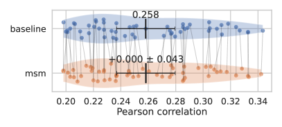
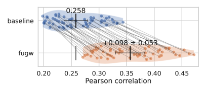
We set $\alpha=0.5$, $\rho=1$ and $\varepsilon=10^{-3}$. Pearson correlation between source and target contrast maps is systematically and significantly increased when aligned using FUGW, as illustrated in Figure 3 where correlation grows by almost 40% from $0.258$ to $0.356$.

Figure 3: Comparison of gains in correlation after inter-subject alignment For each pair of source and target subjects of the dataset, we compute the average Pearson correlation between 30 test contrasts, leading to the (baseline) correspondence score, and compare it with that of the same contrast maps aligned with either MSM (left) or FUGW (right). Correlation gains are much better for FUGW.

We also varied training sets by selecting subsets of training contrasts and find that similar performance on the test set can be achieved regardless of the training data (see Supplementary section A.5 and in particular Supplementary Table S1).

Hyper-parameters selection

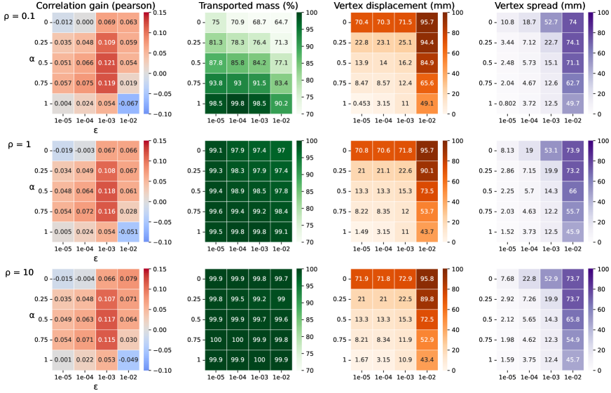
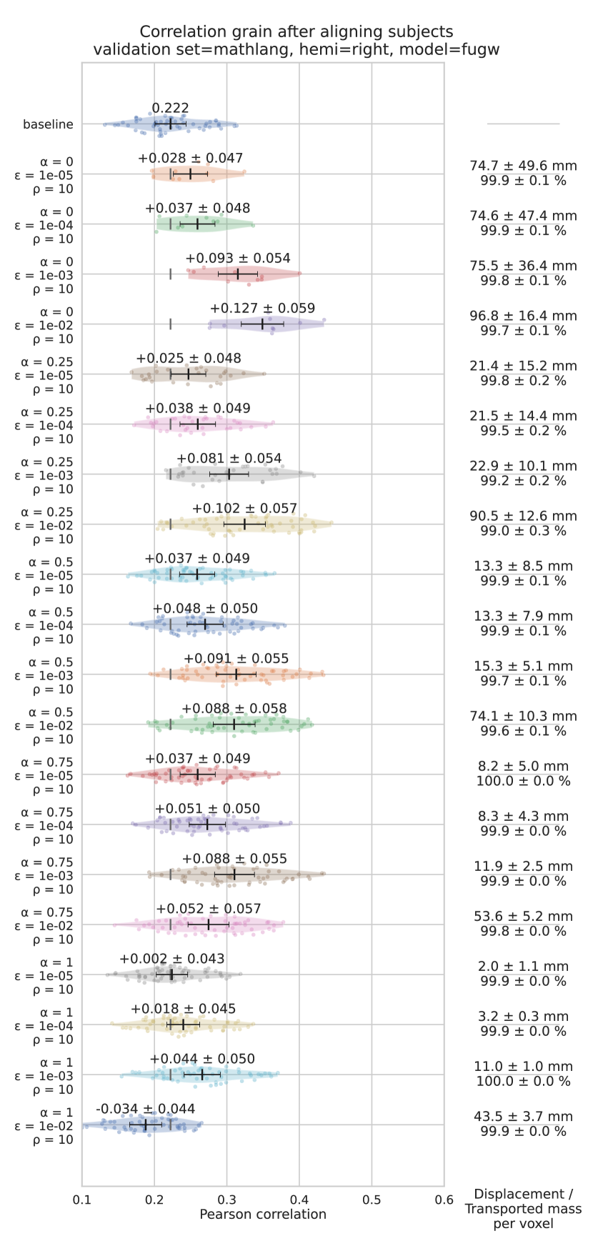
Hyper-parameters used to obtain these results were chosen after running a grid search on $\alpha$, $\varepsilon$ and $\rho$ and evaluating it on the validation dataset. Computation took about 100 hours using 4 Tesla V100-DGXS-32GB GPUs. More precisely, it takes about 4 minutes to compute one coupling between a source and target 10k-vertex hemisphere on a single GPU, when the solver was set to run 10 BCD and 400 Sinkhorn iterations. In comparison, MSM takes about the same time on Intel(R) Xeon(R) CPU E5-2698 v4 @ 2.20GHz CPUs. Results are reported in Figure 4 and provide multiple insights concerning FUGW.

Firstly, without anatomical constraint ($\alpha=0$), source vertices can be matched with target vertices that are arbitrarily far on the cortical sheet. Even though this can significantly increase correlation, it also results in very high vertex displacement values (up to $100mm$). Such couplings are not anatomically plausible. Secondly, without functional information ($\alpha=1$), couplings recover a nearly flawless matching between source and target meshes, so that, when $\varepsilon=10^{-5}$ (ie when we force couplings to find single-vertex-to-single-vertex matches), vertex displacement and spread are close to 0 and correlation is unchanged. Fusing both constraints ($0<\alpha<1$) yields the largest gains in correlation while allowing to compute anatomically plausible reorganizations the cortical sheet between subjects.

The impact of $\rho$ (controlling marginal penalizations) on correlation seems modest, with a slight tendency of increased correlation in unbalanced problems (low $\rho$).

Finally, it is worth noting that a relatively wide range of $\alpha$ and $\rho$ yield comparable gains. The fact that FUGW performance is weakly sensitive to hyper-parameters makes it a good off-the-shelf tool for neuroscientists who wish to derive inter-individual alignments. However, $\varepsilon$ is of dramatic importance in computed results and should be chosen carefully. Vertex spread is a useful metric to choose sensible values of $\varepsilon$; for human data one might consider that it should not exceed $20mm$.

Figure 4: Exploring hyper-parameter space to find relevant couplings Given a transport plan aligning a source and target subject, we evaluate how much this coupling (left) improves correlation between unseen contrast maps of the two subjects, (center left) actually transports data, (center right) moves vertices far from their original location on the cortical surface and (right) spreads vertices on the cortical sheet. We seek plans that maximize correlation gain, while keeping spread and displacement low enough.

Mass redistribution in unbalanced couplings

Unbalanced couplings provide additional information about how functional areas might differ in size between pairs of individuals. This is illustrated in Figure 5, where we observe variation in size of the auditory area between a given pair of individuals. This feature is indeed captured by the difference of mass between subjects (although the displayed contrast was not part of the training set).

Figure 5: Transported mass indicates areas which have to be resized between subjects (Panel A) We show a contrast map from the test set which displays areas showing stronger activation during auditory tasks versus equivalent visual tasks. It shows much more anterior activations on the target subject compared to the source subject. This is consistent with the observation that more mass is present in anterior auditory areas of the source subject than in the target subject (Panel B).

4.2 Experiment 2 - Individual anatomies

Figure 6: Correlation between pairs of subjects is significantly better after alignment on individual anatomies than after projecting subjects onto a common anatomical template

As shown in Figure 6, we obtain correlation gains which are comparable to that of Experiment 1 (about 35% gain) while working on individual meshes. This tends to show that FUGW can compute meaningful alignments between pairs of individuals without the use of an anatomical template, which helps bridge most conceptual impediments listed in Section 1.

Moreover, this opens the way for computation of simple statistics in cohorts of individuals in the absence of a template. Indeed, one can pick an individual of the cohort and use it as a reference subject on which to transport all other individuals. We give an example in Figure S4, showing that FUGW correctly preserved idiosyncrasies of each subject while transporting their functional signal in an anatomically sound way.

4.3 Experiment 3 - Barycenter

In the absence of a proper metric to quantify the correctness of a barycenter, we first qualitatively compare the functional templates obtained with and without alignment. In Figure 7.A, we do so using brain maps taken from the test set. We can see that the barycenter obtained with FUGW yields sharper contrasts and more fine-grained details than the barycenter obtained by per-vertex averaging. We also display in Figure 7.B the result of a one-sample test for the same contrast, which can readily be used for inference. The one-sample test map obtained after alignment to the FUGW template exhibits the same supra-threshold clusters as the original approach, but also some additional spots which were likely lost due to inter-subject variability in the fsaverage5 space. This approach is thus very useful to increase power in group inference. We quantify this result by counting the number of supra-threshold vertices with and without alignment for each contrast map of the test set. Our alignment method significantly finds more such vertices of interest, as shown in Figure 7.C.

Figure 7: FUGW barycenter yields much finer-grained maps than group averages We study the same statistical map as in Figure 1, which contrasts areas of the brain involved in mathematical reasoning. A. These complex maps projected onto the barycenter and averaged show more specific activation patterns than simple group averages, especially in cortical areas exhibiting more variability, such as the prefrontal cortex. B. Deriving a t-test on aligned maps captures the same clusters as the classical approach (plain green circles), but also new clusters in areas where inter-subject variability is high (dotted black circles). Peak t-statistics are also higher with FUGW. C. Ratio of number of activated vertices ($|\text{t-statistic}|\geq 4$) with versus without alignment for each map of the test set. Our method finds significantly more of such vertices ($\text{p-value}=3\cdot 10^{-4}$).

5 Discussion

FUGW can derive meaningful couplings between pairs of subjects without the need of a pre-existing anatomical template. It is well-suited to computing barycenters of individuals, even for small cohorts.

In addition, we have shown clear evidence that FUGW yields gains that cannot be achieved by traditional diffeomorphic registration methods. These methods impose very strong constraints to the displacement field, that may prevent reaching optimal configurations. More deeply, this finding suggests that brain comparison ultimately requires lifting hard regularity constraints on the alignment models, and that two human brains differ by more than a simple continuous surface deformation. However, current results have not shown a strong correlation gain of unbalanced OT compared to balanced OT, likely because the cohort under study is too small. Leveraging datasets such as HCP [43] with a larger number of subjects will help lower the standard error on correlation gain estimates. In this work, we decided to rely on a predefined anatomical template (fsaverage5) to derive functional barycenters. It would be interesting to investigate whether more representative anatomical templates can be learned during the process. This would in particular help to customize templates to different populations or species. Additionally, using an entropic solver introduces a new hyper-parameter $\varepsilon$ that has a strong effect, but is hard to interpret. Future work may replace the scaling algorithm [11] used here by the majorization-minimization one [9], which does not require entropic smoothing. This solution can yield sparse couplings while being orders of magnitude faster, which will prove useful when computing barycenters on large cohorts.

Finally, we plan to make use of FUGW to derive alignments between human and non-human primates without anatomical priors. Indeed, the understanding of given brain mechanisms will benefit from more detailed invasive measurements made on other species only if brains can be matched across species; moreover, this raises the question of features that make the human brain unique, by identifying patterns that have no counterpart in other species. By maximizing the functional alignment between areas, but also allowing for some regions to be massively shrunk or downright absent in one species relative to the other, the present tool could shed an objective light on the important issue of whether and how the language-related areas of the human cortical sheet map onto the architecture of non-human primate brains.

Appendix A Appendix

In the following sections, we provide some additional material to ease the understanding of the underlying alignment problem as well as computational details of solutions of FUGW and FUGW barycenters.

We also show some control experiments during which we used different training data to compute pair-wise alignments and evaluated the proportion of correlation gains that comes from mere signal smoothing.

Eventually, we give details about the IBC dataset (acquisition, preprocessing, fMRI protocols and data splitting).

A.1 Illustration of the alignment problem

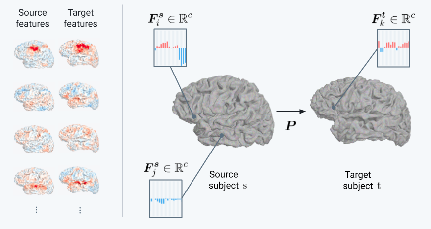
We provide in Fig. S1 a conceptual illustration of the alignment framework for a pair of subjects.

Figure S1: Alignment of two brains using functional signatures Using multiple maps of comparable features (left column) for the source and target subjects, we seek to derive an alignment (also referred to as a coupling) $\bm{P}$ that matches parts of the brain with similar features while preserving the global geometry of the cortex.

A.2 Detailed description of FUGW estimation algorithm

Estimating the unbalanced Gromov Wasserstein (UGW) loss is numerically sensitive to initialization, due to the non-convexity of the problem [39]. Therefore FUGW is a priori non-convex as well, and comparably difficult to estimate. Consequently, following [39], we instead compute a lower bound which we formulate as a bi-convex problem that relies on the joint estimation of two couplings. We provide next a detailed derivation of this estimation procedure, using notations introduced in section 2:

$$\begin{split}\quad\text{FUGW}(\bm{\mathcal{X}^{s}},\bm{\mathcal{X}^{t}})=\quad\inf_{\begin{subarray}{c}\bm{P},\bm{Q}\geq 0\\ \bm{P}=\bm{Q}\end{subarray}}\text{L}_{\theta}(\bm{P},\bm{Q})\quad\geq\inf_{\begin{subarray}{c}\bm{P},\bm{Q}\geq 0\\ m(\bm{P})=m(\bm{Q})\end{subarray}}L_{\theta}(\bm{P},\bm{Q})\quad\triangleq\quad\text{LB-FUGW}(\bm{\mathcal{X}^{s}},\bm{\mathcal{X}^{t}}).\end{split}$$ (S1)

where $m(\bm{P})=\sum_{i,j}\bm{P}_{i,j}$ denotes the mass of $\bm{P}$.

We give the explicit formulation of $\text{L}_{\theta}(\bm{P},\bm{Q})$

$$\begin{split}\text{L}_{\theta}(\bm{P},\bm{Q})\triangleq(1-\alpha)\enspace\text{L}_{\text{W}}(\bm{P},\bm{Q})+\alpha\enspace\text{L}_{\text{GW}}(\bm{P},\bm{Q})+\rho\enspace\text{L}_{\text{U}}(\bm{P},\bm{Q})+\varepsilon\enspace E(\bm{P},\bm{Q}),\end{split}$$ (S2)

where

• $\bm{C}\triangleq\Big{(}||\bm{F^{s}}_{i}-\bm{F^{t}}_{j}||^{2}_{2}\Big{)}_{i,j}\in\mathbb{R}^{2}_{+}$ (feature cost matrix)

• $\bm{G}\triangleq\Big{(}|\bm{D^{s}}_{i,j}-\bm{D^{t}}_{k,l}|\Big{)}_{i,j,k,l}\in\mathbb{R}^{4}_{+}$ (geometry cost matrix)

• $\text{L}_{\text{W}}(\bm{P},\bm{Q})\triangleq\langle\bm{C},\frac{\bm{P}+\bm{Q}}{2}\rangle=\frac{1}{2}(\sum_{i,j}\bm{C}_{i,j}\bm{P}_{i,j}+\sum_{i,j}\bm{C}_{i,j}\bm{Q}_{i,j})$ (Wasserstein)

• $\text{L}_{\text{GW}}(\bm{P},\bm{Q})\triangleq\langle\bm{G},\bm{P}\otimes\bm{Q}\rangle=\sum_{i,j,k,l}\bm{G}_{i,j,k,l}\bm{P}_{i,j}\bm{Q}_{k,l}$ (Gromov-Wasserstein)

• $\text{L}_{\text{U}}(\bm{P},\bm{Q})\triangleq\enspace\text{KL}\Big{(}\bm{P}_{\#1}\otimes\bm{Q}_{\#1}|\bm{w}^{s}\otimes\bm{w}^{s}\Big{)}+\enspace\text{KL}\Big{(}\bm{P}_{\#2}\otimes\bm{Q}_{\#2}|\bm{w}^{t}\otimes\bm{w}^{t}\Big{)}$ (unbalancing)

• $E(\bm{P},\bm{Q})\triangleq\text{KL}\Big{(}\bm{P}\otimes\bm{Q}|(\bm{w^{s}}\otimes\bm{w^{t}})\otimes(\bm{w^{s}}\otimes\bm{w^{t}})\Big{)}$ (entropy)

In particular, we have $\text{L}_{\theta}(\bm{P},\bm{P})=\text{L}_{\theta}(\bm{P})$, which is the objective function of FUGW introduced in Equation 1.

Solver

We provide a Python GPU-based solver for LB-FUGW, using an approach similar to that of [39], which we recall in algorithm S1. More precisely, we alternatively optimize one coupling while keeping the other fixed. This results in two entropic unbalanced OT problems in each iteration, which can be solved using the scaling algorithm [11].

Algorithm S1 Approximation scheme for LB-FUGW

1:$\bm{\mathcal{X}^{s}},\bm{\mathcal{X}^{t}},\rho,\alpha,\varepsilon$.

2:Pair of optimal couplings $(\bm{P},\bm{Q})$.

3:Initialize: $\bm{P}=\bm{Q}=\bm{w^{s}}\otimes\bm{w^{t}}/\sqrt{m(\bm{w^{s}})m(\bm{w^{t}})}$.

4:while $(\bm{P},\bm{Q})$ has not converged do

5:     Calculate: $c_{P}=\text{Cost}(\bm{P},\bm{G},\bm{C},\bm{w^{s}},\bm{w^{t}},\rho,\alpha,\varepsilon)$.

6:     Update: $\bm{Q}\leftarrow\text{Scaling}(c_{P},\bm{w^{s}},\bm{w^{t}},\rho m(\bm{P}),\varepsilon m(\bm{P}))$.

7:     Rescale: $\bm{Q}\leftarrow\sqrt{\frac{m(\bm{P})}{m(\bm{Q})}}\bm{Q}$.

8:     Calculate: $c_{Q}=\text{Cost}(\bm{Q},\bm{G},\bm{C},\bm{w^{s}},\bm{w^{t}},\rho,\alpha,\varepsilon)$.

9:     Update: $\bm{P}\leftarrow\text{Scaling}(c_{Q},\bm{w^{s}},\bm{w^{t}},\rho m(\bm{Q}),\varepsilon m(\bm{Q}))$.

10:     Rescale: $\bm{P}\leftarrow\sqrt{\frac{m(\bm{Q})}{m(\bm{P})}}\bm{P}$.

11:end while

Algorithm S2 Scaling algorithm [11]

1:$\bm{C},\bm{w^{s}},\bm{w^{t}},\rho,\varepsilon$.

2:Optimal coupling $\bm{P}$.

3:Initialize dual vectors: $f=0_{n}\in\mathbb{R}^{n},g=0_{p}\in\mathbb{R}^{p}$.

4:while $(f,g)$ has not converged do

5:     Update: $f=-\frac{\rho}{\rho+\varepsilon}\log\sum_{j}\exp\big{(}g_{j}+\log\bm{w^{t}}_{j}-\frac{\bm{C}_{\cdot,j}}{\varepsilon}\big{)}$.

6:     Update: $g=-\frac{\rho}{\rho+\varepsilon}\log\sum_{i}\exp\big{(}f_{i}+\log\bm{w^{s}}_{i}-\frac{\bm{C}_{i,\cdot}}{\varepsilon}\big{)}$.

7:end while

8:Calculate: $\bm{P}=(\bm{w^{s}}\otimes\bm{w^{t}})\exp\big{(}f\oplus g-\frac{\bm{C}}{\varepsilon}\big{)}$.

Algorithm S3 Cost

1:$\bm{P},\bm{G},\bm{C},\bm{w^{s}},\bm{w^{t}},\rho,\alpha,\varepsilon$.

2:Local cost $c$.

3:Calculate: $\bm{G}\otimes\bm{P}:=\left(\sum_{i,j}\bm{G}_{i,j,k,l}\bm{P}_{i,j}\right)_{k,l}$.

4:Calculate:

$$\begin{split}c:=\alpha\;\bm{G}\otimes\bm{P}+\frac{1-\alpha}{2}\;\bm{C}+\rho\;\langle\log\frac{\bm{P}_{\#1}}{\bm{w^{s}}},\bm{P}_{\#1}\rangle+\rho\;\langle\log\frac{\bm{P}_{\#2}}{\bm{w^{t}}},\bm{P}_{\#2}\rangle+\varepsilon\;\langle\log\frac{\bm{P}}{\bm{w^{s}}\otimes\bm{w^{t}}},\bm{P}\rangle\end{split}$$

Here, the notations $\otimes$ and $\oplus$ denote the Kronecker product and sum, respectively. The exponential, division and logarithm operations are all element-wise. The scalar product is denoted by $\langle\cdot,\cdot\rangle$.

In practice, we observe that the two couplings of LB-FUGW are numerically equal, so it is enough to choose, for example, the first one, as alignment between source and target signals.

A.3 Detailed description of FUGW barycenter estimation

FUGW-barycenter algorithm, described in Algorithm S4, alternates between computing mappings from subjects to the barycenter, and updating the barycenter. This corresponds to a block coordinate descent on the barycenter estimation. The first step simply uses the previously introduced solver. The second one takes advantage of the fact that the objective function introduced in S1 is differentiable in $\bm{F^{B}}$ and $\bm{D^{B}}$, and the two couplings of LB-FUGW are numerically equal. This yields a closed form for $\bm{F^{B}}$ and $\bm{D^{B}}$, as a function of $\bm{P^{s,B}}$ and $\bm{\mathcal{X}^{s}}$. We note that, during the barycenter estimation, the weight $\bm{w^{B}}$ is always fixed as uniform distribution.

Algorithm S4 LB-FUGW barycenter

1:$(\bm{\mathcal{X}^{s}})_{s\in\mathcal{S}},\rho,\alpha,\varepsilon$.

2: Individual couplings $(\bm{P^{s,B}})_{s\in\mathcal{S}}$, barycenter $\bm{\mathcal{X}^{B}}$.

3:Initialize: $\bm{F^{B}}=\bm{\mathbb{I}_{k}}$; $\bm{D^{B}}=\bm{\mathbb{0}_{k}}$.

4:while $\bm{\mathcal{X}^{B}}=(\bm{F^{B}},\bm{D^{B}},\bm{w^{B}})$ has not converged do

5:     Draw $\widetilde{S}$ subset of $S$.

6:     for $s\in\widetilde{S}$ do $\triangleright$ fixed $\bm{\mathcal{X}^{B}}$

7:         Align: $\bm{P^{s,B}}\leftarrow\text{LB-FUGW}(\bm{\mathcal{X}^{s}},\bm{\mathcal{X}^{B}},\rho,\alpha,\varepsilon)$.

8:     end for

9:     Update $\bm{F^{B}}$, $\bm{D^{B}}$: $\triangleright$ fixed $\bm{P^{s,B}}$

$$\bm{F^{B}}=\frac{1}{|\widetilde{S}|}\sum_{s\in\widetilde{S}}\text{diag}\left(\frac{1}{\bm{P^{s,B}}_{\#2}}\right)(\bm{P^{s,B}})^{\top}\bm{F^{s}}\;\text{ and }\;\bm{D_{B}}=\frac{1}{|\widetilde{S}|}\sum_{s\in\widetilde{S}}\frac{(\bm{P^{s,B}})^{\top}\bm{D^{s}}\bm{P^{s,B}}}{\bm{P^{s,B}}_{\#2}(\bm{P^{s,B}}_{\#2})^{\top}}.$$

10:end while

A.4 Implementation details

MSM configuration

We use the default configuration of MSM and vary parameter lambda so as to obtain the best gains in correlation on the test set. We use the same value of lambda at each step of MSM and eventually set it to 0.1 after a cross validated grid search.

Correlation gain variability when aligning pairs of subjects

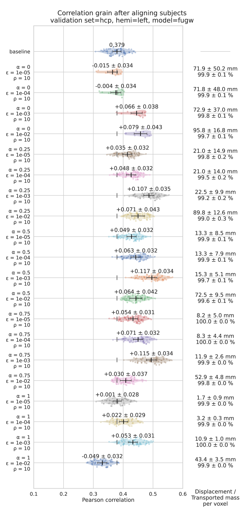
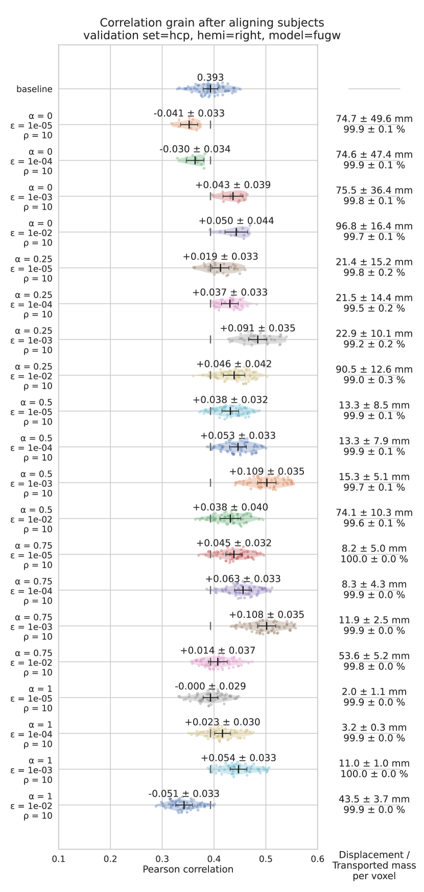
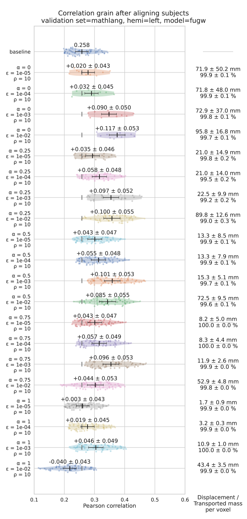
Figures S2 and S3 show correlation gains on the validation and test sets respectively when aligning pairs of subjects from the IBC dataset. Subjects’ data was previously projected onto fsaverage5. These figures provide us with a better understanding of the standard error and consistency of these gains. Moreover, they show that selection of the best set of hyper-parameters is robust to changing the validation data.

Figure S2: Detailed correlation gains on the validation set (HCP tasks), in the balanced case Each line represents a FUGW model trained with different hyper-parameters. Each dot represents the mean correlation between contrast maps of the HCP protocol for a given pair of IBC subjects. We compare the average correlation with that of the baseline (top row) where subjects were simply projected on fsaverage5. Models for the left hemisphere and right hemisphere are shown respectively on the left and right side.

Figure S3: Detailed correlation gains on the test set (Mathlang tasks) in the balanced case Similarly to Figure S2, each line represents a FUGW model trained with different hyper-parameters. Each dot represents the mean correlation between contrast maps of the Mathlang protocol for a given pair of IBC subjects. We compare the average correlation with that of the baseline (top row) where subjects were simply projected on fsaverage5. Models for the left hemisphere and right hemisphere are shown respectively on the left and right side.

Mesh resolution reduction

As mentioned in the core of this paper, aligning meshes with high resolutions can lead to dealing with matrices which won’t fit on GPUs. This is typically the case when trying to align two fsaverage7 hemispheres (160k vertices each) instead of fsaverage5 hemispheres (10k vertices each).

In order to reduce the number $n$ of aligned vertices, we first group them into small clusters using Ward’s algorithm using a method described in [41]. In essence, this method iteratively groups adjacent vertices of a given individual based on feature similarity until $I$ clusters have been formed. Then, for a given cluster $u_{i}$ of the source subject $s$, we define its functional signal $\bm{\hat{F}^{s}}_{u_{i}}$ as the mean functional signal of vertices which belong to this cluster. Moreover, for two given clusters $u_{i}$ and $u_{j}$ of subject $s$, we define the anatomical distance $\bm{\hat{D}^{s}}_{u_{i},u_{j}}$ between $u_{i}$ and $u_{j}$ as the mean geodesic distance between all pairs of vertices between the two clusters (akin to an Energy distance). Eventually, we derive analogous objects $\bm{\hat{F}^{t}}$ and $\bm{\hat{D}^{t}}$ for the target subject $t$, and end up in a configuration comparable to that of Experiment 1.

$$\bm{\hat{F}^{s}}_{u_{i}}\triangleq\frac{1}{|u_{i}|}\sum_{k\in u_{i}}\bm{F^{s}}_{k}\in\mathbb{R}^{c}$$

$$\bm{\hat{D}^{s}}_{u_{i},u_{j}}\triangleq\frac{1}{|u_{i}|\cdot|u_{j}|}\sum_{k\in u_{i},l\in u_{j}}\bm{D}^{s}_{k,l}$$

Alignment to individual anatomy

We qualitatively control that alignments derived between individuals on their individual anatomies make sense in Figure S4.

Figure S4: Transporting individual maps onto a reference subject FUGW can help bridge the absence of template anatomies and derive pairs of alignments such that all individuals of the cohort are comparable. We display a map taken from the test set contrasting areas activated during mathematical reasoning against areas activated for other stimuli of the protocol.

A.5 Control experiments

Controlling for smoothing effect increasing correlation

Alignments computed with FUGW are not always vertex-to-vertex alignments. Indeed, a single vertex from the source subject $s$ can be associated with many vertices in the target subject $t$. In fact, $\bm{P^{s,t}}_{i}$ represents the relative importance of each match. The hyper-parameter $\varepsilon$ controls the entropy of $\bm{P^{s,t}}$, which is in direct link with the spread of vertices that we use as a measure for how many target vertices are matched with source vertices.

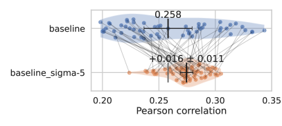
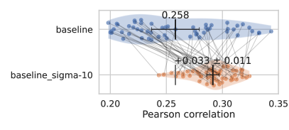
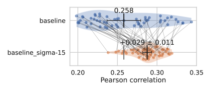
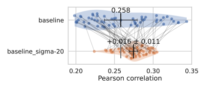
Since smoothing signal on the source subject can reduce noise and increase correlation to target data, we measure the correlation gain induced by applying a gaussian kernel to the source signal. This allows us to show that only a minor proportion of correlation gains induced by FUGW can come from this smoothing effect. Figure S5 shows this for kernels of 5mm, 10mm, 15mm and 20mm of standard deviation respectively. We see that correlation increases significantly less than when using FUGW (0.03 vs 0.12 correlation gain respectively). Moreover, one notices that even though correlation increases for pairs of subjects with a low initial correlation, it decreases for pairs with a high initial correlation. On the contrary, FUGW increases correlation for all pairs of subjects.

Figure S5: Comparison of gains in correlation after Gaussian blurring We compare correlation between subjects after the source subject’s functional data has been smoothed with a Gaussian kernel of standard deviation 5mm (top left), 10mm (top right), 15mm (bottom left) and 20mm (bottom right)

Different training sets yield comparable correlation gains

While we leverage all IBC maps to derive our couplings, we show that the presented results hold when using a much smaller training dataset. In particular, we observe similar correlation gains when using only the 57 maps of the Archi protocol for training (see Table S3). It takes about one hour per subject to acquire these maps, which we advocate is a reasonable amount of time to build a training set dedicated to align subjects within a given cohort (and possibly across cohorts). Finally, we train both FUGW and MSM with lower-dimensional versions of the previous datasets. To do so, given a pair of subjects $(s,t)$ to be aligned, we fit a PCA on the left out subjects, project the data of subjects to be aligned on these components, and keep the first 20 components only. For both models, correlation gains remained unchanged.

More explicitly, we test the 4 following training sets:

• ALL-MATH: all contrast maps of IBC except contrasts from the Mathlang protocol (369 features per subject)

• ALL-MATH PCA: principal components fitted on ALL-MATH for all IBC subjects except $s$ and $t$ (20 features)

• ARCHI: all contrast maps from the Archi protocol of IBC (57 features)

• ARCHI PCA: principal components fitted on ARCHI for all subjects except $s$ and $t$ (20 features)

Training set	FUGW	MSM
ALL-MATH	0.12	0.01
ALL-MATH PCA	0.11	0.02
ARCHI	0.10	0.02
ARCHI PCA	0.11	0.01

Table S1: Gain in Pearson correlation of aligned contrast maps from the Mathlang protocol compared to the baseline The original correlation (baseline) is 0.258

Using naturalistic stimuli to derive alignments with FUGW

This experiment’s setup is similar to that of Experiment 1: Using training features to first derive OT couplings, we then use the latter to assess correlation gains between subjects’s feature maps before and after subjects have been aligned. Naturalistic stimuli datasets include Raiders of the Lost Ark, short video clips and auditory stimuli from The Little Prince respectively adapted from [21, 27, 8]. Here, for each naturalistic dataset, we leverage work from [34] to derive the first $m=20$ components of a fitted shared response model. Share response models seek to find a common dictionary $\bm{K}$ of activation patterns across subjects $s\in S$ and to derive a mapping $\bm{W^{s}}$ with $m$ orthogonal components that projects each individual’s data onto this common space:

$$\operatorname*{arg\,min}_{\begin{subarray}{c}\bm{K},\bm{W^{s}}\\ \text{s.t. }\bm{(W^{s})^{T}\cdot W^{s}=I_{m}}\end{subarray}}\sum_{s\in S}||\bm{F^{s}}-\bm{W^{s}}\bm{K}||^{2}$$

These $\bm{W^{s}}$ are then used for alignment.

Results are reported in Table S2 and show that using datasets which are 20 times less time-consuming than that of Experiment 1 can already yield significant correlation gain on unseen task data.

Table S2: Acquisition time (AT) and correlation gain on the left hemisphere (CG) per training set (baseline correlation = 0.258)

Training set	Type	AT (min)	CG (Pearson)
All-MATH	tasks	2000	0.118
Clips	movie	100	0.017
Raiders	movie	115	0.046
The Little Prince	movie	100	0.009

Transporting myelin maps shows mild effect

Leveraging transport plans computed using fMRI data from Experiment 1, we transport myelin maps – approximated through T1 / T2 ratio maps – from the source subject to the target subject. We compare the correlation of the unaligned source and target maps with the correlation of the transported and target maps. As illustrated in Figure S6, correlation gain is barely significant.

Figure S6: Comparison of gains in correlation after inter-subject alignment for myelin maps For each pair of source and target subjects of the IBC dataset, we compute the average Pearson correlation between myelin maps – approximated using T1/T2 ratios – for the left (left panel) and right (right panel) hemispheres. Correlation gains are not significant.

Before computing correlation between aforementioned maps, we discarded vertices located in the cortical wall, as they mostly contain spurious values. To do so, we they their value to the median of values of vertices which do not belong to the cortical wall. In order to determine which vertices belong to the wall, we used the Destrieux atlas [13].

Eventually, we advocate that little gain can be obtained when better aligning myelin maps, since they are already very stable across human subjects as shown in Figure S7.

Figure S7: Myelin maps (approximated using T1/T2 ratio maps) are very consistent across IBC participants

A.6 Dataset description

The presented experiments rely on the Individual Brain Charting (IBC) dataset. A detailed description of the preprocessing pipeline of the IBC data is provided in [32]. Raw data were preprocessed using PyPreprocess .

All fMRI images, i.e. GE-EPI volumes, were collected twice with reversed phase-encoding directions, resulting in pairs of images with distortions going in opposite directions. Susceptibility-induced off-resonance field was estimated from the two Spin-Echo EPI volumes in reversed phase-encoding directions. The images were corrected based on the estimated deformation model. Details about the method can be found in [3].

Further, the GE-EPI volumes were aligned to each other within every participant. A rigid-body transformation was employed, in which the average volume of all images was used as reference [17]. The anatomical and motion-corrected fMRI images were given as input to FreeSurfer v6.0.0, in order to extract meshes of the tissue interfaces and the sampling of functional activation on these meshes, as described in [42]. The corresponding maps were then resampled to the fsaverage7 (high resolution, 163k nodes per hemisphere) and fsaverage5 (low resolution, 10k nodes per hemisphere) templates of FreeSurfer [16].

FMRI data were analyzed using the General Linear Model. Regressors of the model were designed to capture variations in BOLD response strictly following stimulus timing specifications. They were estimated through the convolution of boxcar functions, that represent per-condition stimulus occurrences, with the canonical Hemodynamic Response Function (HRF). To build such models, paradigm descriptors grouped in triplets (i.e. onset time, duration and trial type) according to BIDS Specification were determined from the log files’ registries generated by the stimulus-delivery software. To account for small fluctuations in the latency of the HRF peak response, additional regressors were computed based on the convolution of the same task-conditions profile with the time derivative of the HRF. Nuisance regressors were also added to the design matrix in order to minimize the final residual error. To remove signal variance associated with spurious effects arising from movements, six temporal regressors were defined for the motion parameters. Further, the first five principal components of the signal, extracted from voxels showing the $5\%$ highest variance, were also regressed to capture physiological noise [7].

In addition, a discrete-cosine basis was included for high-pass filtering (cutoff=$\frac{1}{128}\textrm{Hz}$). Model specification was implemented using Nilearn v0.8.1 [2], a Python library for statistical learning on neuroimaging data (https://nilearn.github.io).

In tables S3, S4 and S5, we give the explicit list of contrast and condition maps used for training, validation and testing respectively.

Table S3: Training data This dataset comprises a wide variety of tasks: motor, visual, auditory, relational, linguistic, etc.

Training data
Task	Condition / Contrast
ArchiEmotional	expression_control
ArchiEmotional	expression_gender
ArchiEmotional	expression_gender-control
ArchiEmotional	expression_intention
ArchiEmotional	expression_intention-control
ArchiEmotional	expression_intention-gender
ArchiEmotional	face_control
ArchiEmotional	face_gender
ArchiEmotional	face_gender-control
ArchiEmotional	face_trusty
ArchiEmotional	face_trusty-control
ArchiEmotional	face_trusty-gender
ArchiEmotional	trusty_and_intention-control
ArchiEmotional	trusty_and_intention-gender
ArchiSocial	false_belief-mechanistic
ArchiSocial	false_belief-mechanistic_audio
ArchiSocial	false_belief-mechanistic_video
ArchiSocial	false_belief_audio
ArchiSocial	false_belief_video
ArchiSocial	mechanistic_audio
ArchiSocial	mechanistic_video
ArchiSocial	non_speech_sound
ArchiSocial	speech-non_speech
ArchiSocial	speech_sound
ArchiSocial	triangle_mental
ArchiSocial	triangle_mental-random
ArchiSocial	triangle_random
ArchiSpatial	grasp-orientation
ArchiSpatial	hand-side
ArchiSpatial	object_grasp
ArchiSpatial	object_orientation
ArchiSpatial	rotation_hand
ArchiSpatial	rotation_side
ArchiSpatial	saccades
ArchiStandard	audio_computation
ArchiStandard	audio_left_button_press
ArchiStandard	audio_right_button_press
ArchiStandard	audio_sentence
ArchiStandard	cognitive-motor
ArchiStandard	computation
ArchiStandard	computation-sentences
ArchiStandard	horizontal-vertical
ArchiStandard	horizontal_checkerboard
ArchiStandard	left-right_button_press
ArchiStandard	listening-reading
ArchiStandard	motor-cognitive
ArchiStandard	reading-checkerboard
ArchiStandard	reading-listening
ArchiStandard	right-left_button_press
ArchiStandard	sentences
ArchiStandard	sentences-computation
ArchiStandard	vertical-horizontal
ArchiStandard	vertical_checkerboard
ArchiStandard	video_computation
ArchiStandard	video_left_button_press
ArchiStandard	video_right_button_press
ArchiStandard	video_sentence
Attention	double_congruent
Attention	double_cue
Attention	double_incongruent
Attention	double_incongruent-double_congruent
Attention	incongruent-congruent
Attention	spatial_congruent
Attention	spatial_cue
Attention	spatial_cue-double_cue
Attention	spatial_incongruent
Attention	spatial_incongruent-spatial_congruent
Audi	alphabet
Audi	alphabet-silence
Audi	animals
Audi	animals-silence
Audi	cough
Audi	cough-silence
Audi	environment
Audi	environment-silence
Audi	human
Audi	human-silence
Audi	laugh
Audi	laugh-silence
Audi	music
Audi	music-silence
Audi	reverse
Audi	reverse-silence
Audi	silence
Audi	speech
Audi	speech-silence
Audi	suomi
Audi	suomi-silence
Audi	tear
Audi	tear-silence
Audi	yawn
Audi	yawn-silence
Audio	animal
Audio	animal-others
Audio	animal-silence
Audio	mean-silence
Audio	music
Audio	music-others
Audio	music-silence
Audio	nature
Audio	nature-others
Audio	nature-silence
Audio	speech
Audio	speech-others
Audio	speech-silence
Audio	tool
Audio	tool-others
Audio	tool-silence
Audio	voice
Audio	voice-others
Audio	voice-silence
Bang	no_talk
Bang	talk
Bang	talk-no_talk
ColumbiaCards	gain
ColumbiaCards	loss
ColumbiaCards	num_loss_cards
Discount	amount
Discount	delay
DotPatterns	correct_cue-incorrect_cue
DotPatterns	correct_cue_correct_probe
DotPatterns	correct_cue_incorrect_probe
DotPatterns	correct_cue_incorrect_probe-correct_cue_correct_probe
DotPatterns	correct_cue_incorrect_probe-incorrect_cue_correct_probe
DotPatterns	cue
DotPatterns	incorrect_cue_correct_probe
DotPatterns	incorrect_cue_incorrect_probe
DotPatterns	incorrect_cue_incorrect_probe-correct_cue_incorrect_probe
DotPatterns	incorrect_cue_incorrect_probe-incorrect_cue_correct_probe
DotPatterns	incorrect_probe-correct_probe
EmotionalPain	emotional-physical_pain
EmotionalPain	emotional_pain
EmotionalPain	physical_pain
Enumeration	enumeration_constant
Enumeration	enumeration_linear
Enumeration	enumeration_quadratic
Lec1	pseudoword
Lec1	pseudoword-random_string
Lec1	random_string
Lec1	word
Lec1	word-pseudoword
Lec1	word-random_string
Lec2	attend
Lec2	attend-unattend
Lec2	unattend
MCSE	high-low_salience
MCSE	high_salience_left
MCSE	high_salience_right
MCSE	low+high_salience
MCSE	low-high_salience
MCSE	low_salience_left
MCSE	low_salience_right
MCSE	salience_left-right
MCSE	salience_right-left
MTTNS	northside-southside_event
MTTNS	sn_after-before_event
MTTNS	sn_after_event
MTTNS	sn_all_event_response
MTTNS	sn_all_space-time_cue
MTTNS	sn_all_space_cue
MTTNS	sn_all_time-space_cue
MTTNS	sn_all_time_cue
MTTNS	sn_average_event
MTTNS	sn_average_reference
MTTNS	sn_before-after_event
MTTNS	sn_before_event
MTTNS	sn_northside_event
MTTNS	sn_southside_event
MTTNS	sn_space-time_event
MTTNS	sn_space_event
MTTNS	sn_time-space_event
MTTNS	sn_time_event
MTTNS	southside-northside_event
MTTWE	eastside-westside_event
MTTWE	we_after-before_event
MTTWE	we_after_event
MTTWE	we_all_event_response
MTTWE	we_all_space-time_cue
MTTWE	we_all_space_cue
MTTWE	we_all_time-space_cue
MTTWE	we_all_time_cue
MTTWE	we_average_event
MTTWE	we_average_reference
MTTWE	we_before-after_event
MTTWE	we_before_event
MTTWE	we_eastside_event
MTTWE	we_space-time_event
MTTWE	we_space_event
MTTWE	we_time-space_event
MTTWE	we_time_event
MTTWE	we_westside_event
MTTWE	westside-eastside_event
MVEB	2_letters_different
MVEB	2_letters_different-same
MVEB	2_letters_same
MVEB	4_letters_different
MVEB	4_letters_different-same
MVEB	4_letters_same
MVEB	6_letters_different
MVEB	6_letters_different-2_letters_different
MVEB	6_letters_different-same
MVEB	6_letters_same
MVEB	letter_occurrence_response
MVIS	2_dots-2_dots_control
MVIS	4_dots-4_dots_control
MVIS	6_dots-2_dots
MVIS	6_dots-6_dots_control
MVIS	dot_displacement_response
MVIS	dots-control
Moto	finger_left-fixation
Moto	finger_right-fixation
Moto	foot_left-fixation
Moto	foot_right-fixation
Moto	hand_left-fixation
Moto	hand_right-fixation
Moto	instructions
Moto	saccade-fixation
Moto	tongue-fixation
PainMovie	movie_mental
PainMovie	movie_mental-pain
PainMovie	movie_pain
Preference	face-others
Preference	food-others
Preference	house-others
Preference	painting-others
Preference	preference_constant
Preference	preference_linear
Preference	preference_quadratic
PreferenceFaces	face_constant
PreferenceFaces	face_linear
PreferenceFaces	face_quadratic
PreferenceFood	food_constant
PreferenceFood	food_linear
PreferenceFood	food_quadratic
PreferenceHouses	house_constant
PreferenceHouses	house_linear
PreferenceHouses	house_quadratic
PreferencePaintings	painting_constant
PreferencePaintings	painting_linear
PreferencePaintings	painting_quadratic
RSVPLanguage	complex
RSVPLanguage	complex-consonant_string
RSVPLanguage	complex-simple
RSVPLanguage	consonant_string
RSVPLanguage	jabberwocky
RSVPLanguage	jabberwocky-consonant_string
RSVPLanguage	jabberwocky-pseudo
RSVPLanguage	probe
RSVPLanguage	pseudo-consonant_string
RSVPLanguage	pseudoword_list
RSVPLanguage	sentence-consonant_string
RSVPLanguage	sentence-jabberwocky
RSVPLanguage	sentence-pseudo
RSVPLanguage	sentence-word
RSVPLanguage	simple
RSVPLanguage	simple-consonant_string
RSVPLanguage	word-consonant_string
RSVPLanguage	word-pseudo
RSVPLanguage	word_list
SelectiveStopSignal	go_critical
SelectiveStopSignal	go_critical-stop
SelectiveStopSignal	go_noncritical
SelectiveStopSignal	go_noncritical-ignore
SelectiveStopSignal	ignore
SelectiveStopSignal	ignore-stop
SelectiveStopSignal	stop
SelectiveStopSignal	stop-ignore
Self	correct_rejection
Self	encode_other
Self	encode_self
Self	encode_self-other
Self	false_alarm
Self	instructions
Self	recognition_hit
Self	recognition_hit-correct_rejection
Self	recognition_other_hit
Self	recognition_self-other
Self	recognition_self_hit
StopSignal	go
StopSignal	stop
StopSignal	stop-go
Stroop	congruent
Stroop	incongruent
Stroop	incongruent-congruent
TheoryOfMind	belief
TheoryOfMind	belief-photo
TheoryOfMind	photo
TwoByTwo	cue_switch-stay
TwoByTwo	cue_taskstay_cuestay
TwoByTwo	cue_taskstay_cueswitch
TwoByTwo	cue_taskswitch_cuestay
TwoByTwo	cue_taskswitch_cueswitch
TwoByTwo	stim_taskstay_cuestay
TwoByTwo	stim_taskstay_cueswitch
TwoByTwo	stim_taskswitch_cuestay
TwoByTwo	stim_taskswitch_cueswitch
TwoByTwo	task_switch-stay
VSTM	vstm_constant
VSTM	vstm_linear
VSTM	vstm_quadratic
Visu	animal
Visu	animal-scrambled
Visu	characters
Visu	characters-scrambled
Visu	face
Visu	face-scrambled
Visu	house
Visu	house-scrambled
Visu	pseudoword
Visu	pseudoword-scrambled
Visu	scene
Visu	scene-scrambled
Visu	scrambled
Visu	target_fruit
Visu	tool
Visu	tool-scrambled
WardAndAllport	ambiguous-unambiguous
WardAndAllport	intermediate-direct
WardAndAllport	move_ambiguous_direct
WardAndAllport	move_ambiguous_intermediate
WardAndAllport	move_unambiguous_direct
WardAndAllport	move_unambiguous_intermediate
WardAndAllport	planning_ambiguous_direct
WardAndAllport	planning_ambiguous_intermediate
WardAndAllport	planning_unambiguous_direct
WardAndAllport	planning_unambiguous_intermediate

Table S4: Validation data

Validation data
Task	Condition / Contrast
HcpEmotion	face
HcpEmotion	face-shape
HcpEmotion	shape
HcpEmotion	shape-face
HcpGambling	punishment
HcpGambling	punishment-reward
HcpGambling	reward
HcpGambling	reward-punishment
HcpLanguage	math
HcpLanguage	math-story
HcpLanguage	story
HcpLanguage	story-math
HcpMotor	cue
HcpMotor	left_foot
HcpMotor	left_foot-avg
HcpMotor	left_hand
HcpMotor	left_hand-avg
HcpMotor	right_foot
HcpMotor	right_foot-avg
HcpMotor	right_hand
HcpMotor	right_hand-avg
HcpMotor	tongue
HcpMotor	tongue-avg
HcpRelational	match
HcpRelational	relational
HcpRelational	relational-match
HcpSocial	mental
HcpSocial	mental-random
HcpSocial	random
HcpWm	0back-2back
HcpWm	0back_body
HcpWm	0back_face
HcpWm	0back_place
HcpWm	0back_tools
HcpWm	2back-0back
HcpWm	2back_body
HcpWm	2back_face
HcpWm	2back_place
HcpWm	2back_tools
HcpWm	body-avg
HcpWm	face-avg
HcpWm	place-avg
HcpWm	tools-avg

Table S5: Test data

Test data
Task	Condition / Contrast
MathLanguage	arithmetic_fact-othermath
MathLanguage	arithmetic_fact_auditory
MathLanguage	arithmetic_fact_visual
MathLanguage	arithmetic_principle-othermath
MathLanguage	arithmetic_principle_auditory
MathLanguage	arithmetic_principle_visual
MathLanguage	auditory-visual
MathLanguage	colorlessg-wordlist
MathLanguage	colorlessg_auditory
MathLanguage	colorlessg_visual
MathLanguage	context-general
MathLanguage	context-theory_of_mind
MathLanguage	context_auditory
MathLanguage	context_visual
MathLanguage	general-colorlessg
MathLanguage	general_auditory
MathLanguage	general_visual
MathLanguage	geometry-othermath
MathLanguage	geometry_fact_auditory
MathLanguage	geometry_fact_visual
MathLanguage	math-nonmath
MathLanguage	nonmath-math
MathLanguage	theory_of_mind-context
MathLanguage	theory_of_mind-general
MathLanguage	theory_of_mind_and_context-general
MathLanguage	theory_of_mind_auditory
MathLanguage	theory_of_mind_visual
MathLanguage	visual-auditory
MathLanguage	wordlist_auditory
MathLanguage	wordlist_visual

References

- [1] Alexandre Abraham et al. “Machine learning for neuroimaging with scikit-learn” In Frontiers in Neuroinformatics 8, 2014 URL: https://www.frontiersin.org/article/10.3389/fninf.2014.00014
- [2] Alexandre Abraham et al. “Machine learning for neuroimaging with scikit-learn” In Front Neuroinform 8, 2014, pp. 14 URL: https://doi.org/10.3389/fninf.2014.00014
- [3] Jesper L.R. Andersson, Stefan Skare and John Ashburner “How to correct susceptibility distortions in spin-echo echo-planar images: application to diffusion tensor imaging” In Neuroimage 20.2, 2003, pp. 870–888 URL: http://doi.org/10.1016/S1053-8119(03)00336-7
- [4] B.B. Avants, C.L. Epstein, M. Grossman and J.C. Gee “Symmetric diffeomorphic image registration with cross-correlation: Evaluating automated labeling of elderly and neurodegenerative brain” In Medical Image Analysis 12.1, 2008, pp. 26–41 DOI: 10.1016/j.media.2007.06.004
- [5] Thomas BAZEILLE, Hugo Richard, Hicham Janati and Bertrand Thirion “Local Optimal Transport for Functional Brain Template Estimation” In IPMI 2019 - 26th International Conference on Information Processing in Medical Imaging, 2019 DOI: 10.1007/978-3-030-20351-1_18
- [6] Thomas Bazeille et al. “An empirical evaluation of functional alignment using inter-subject decoding” In NeuroImage 245, 2021, pp. 118683 DOI: 10.1016/j.neuroimage.2021.118683
- [7] Yashar Behzadi, Khaled Restom, Joy Liau and Thomas T. Liu “A component based noise correction method (CompCor) for {BOLD} and perfusion based fMRI” In Neuroimage 37.1, 2007, pp. 90–101 URL: https://doi.org/10.1016/j.neuroimage.2007.04.042
- [8] Shohini Bhattasali et al. “Localising memory retrieval and syntactic composition: an fMRI study of naturalistic language comprehension” In Language, Cognition and Neuroscience 34.4 Taylor & Francis, 2019, pp. 491–510
- [9] Laetitia Chapel et al. “Unbalanced Optimal Transport through Non-negative Penalized Linear Regression” In arXiv:2106.04145 [cs, math, stat], 2021 arXiv: http://arxiv.org/abs/2106.04145
- [10] Po-Hsuan (Cameron) Chen et al. “A Reduced-Dimension fMRI Shared Response Model” In Advances in Neural Information Processing Systems 28 Curran Associates, Inc., 2015 URL: https://proceedings.neurips.cc/paper/2015/file/b3967a0e938dc2a6340e258630febd5a-Paper.pdf
- [11] Lenaic Chizat, Gabriel Peyré, Bernhard Schmitzer and François-Xavier Vialard “Unbalanced Optimal Transport: Dynamic and Kantorovich Formulation” In arXiv:1508.05216 [math], 2019 arXiv: http://arxiv.org/abs/1508.05216
- [12] Anders M. Dale, Bruce Fischl and Martin I. Sereno “Cortical Surface-Based Analysis: I. Segmentation and Surface Reconstruction”, 1999, pp. 179–194 DOI: 10.1006/nimg.1998.0395
- [13] Christophe Destrieux, Bruce Fischl, Anders Dale and Eric Halgren “Automatic parcellation of human cortical gyri and sulci using standard anatomical nomenclature” In NeuroImage 53.1, 2010, pp. 1–15 DOI: 10.1016/j.neuroimage.2010.06.010
- [14] Nicole Eichert et al. “Cross-species cortical alignment identifies different types of anatomical reorganization in the primate temporal lobe” Publisher: eLife Sciences Publications, Ltd In eLife 9, 2020, pp. e53232 DOI: 10.7554/eLife.53232
- [15] Bruce Fischl “FreeSurfer” In NeuroImage 62.2, 20 YEARS OF fMRI, 2012, pp. 774–781 DOI: 10.1016/j.neuroimage.2012.01.021
- [16] Bruce Fischl, Martin I. Sereno, Roger B.H. Tootell and Anders M. Dale “High-resolution intersubject averaging and a coordinate system for the cortical surface” In Hum Brain Mapp 8.4, 1999, pp. 272–284 URL: https://doi.org/10.1002/(SICI)1097-0193(1999)8:4%3C272::AID-HBM10%3E3.0.CO;2-4
- [17] K.J. Friston, C.D. Frith, R.S.J. Frackowiak and R. Turner “Characterizing Dynamic Brain Responses with fMRI: a Multivariate Approach” In Neuroimage 2.2, 1995, pp. 166–172 URL: https://doi.org/10.1006/nimg.1995.1019
- [18] Matthew F Glasser et al. “A multi-modal parcellation of human cerebral cortex” In Nature 536.7615 nature.com, 2016, pp. 171–178
- [19] Alexandre Gramfort, Gabriel Peyré and Marco Cuturi “Fast Optimal Transport Averaging of Neuroimaging Data” arXiv, 2015 DOI: 10.48550/ARXIV.1503.08596
- [20] J. Guntupalli et al. “A Model of Representational Spaces in Human Cortex” Publisher: Oxford Academic In Cerebral Cortex 26.6, 2016, pp. 2919–2934 DOI: 10.1093/cercor/bhw068
- [21] James V. Haxby et al. “A common, high-dimensional model of the representational space in human ventral temporal cortex” In Neuron 72.2, 2011, pp. 404–416 DOI: 10.1016/j.neuron.2011.08.026
- [22] Matthias Liero, Alexander Mielke and Giuseppe Savaré “Optimal Entropy-Transport problems and a new Hellinger–Kantorovich distance between positive measures” In Inventiones mathematicae 211.3, 2018, pp. 969–1117 DOI: 10.1007/s00222-017-0759-8
- [23] Rogier B Mars et al. “Whole brain comparative anatomy using connectivity blueprints” Publisher: eLife Sciences Publications, Ltd In eLife 7, 2018, pp. e35237 DOI: 10.7554/eLife.35237
- [24] Facundo Memoli “On the use of Gromov-Hausdorff Distances for Shape Comparison” Accepted: 2014-01-29T16:52:11Z ISSN: 1811-7813 The Eurographics Association, 2007 DOI: 10.2312/SPBG/SPBG07/081-090
- [25] Facundo Mémoli “Gromov–Wasserstein Distances and the Metric Approach to Object Matching” In Foundations of Computational Mathematics 11.4, 2011, pp. 417–487 DOI: 10.1007/s10208-011-9093-5
- [26] Franz-Xaver Neubert et al. “Comparison of human ventral frontal cortex areas for cognitive control and language with areas in monkey frontal cortex” In Neuron 81.3, 2014, pp. 700–713 DOI: 10.1016/j.neuron.2013.11.012
- [27] Shinji Nishimoto et al. “Reconstructing visual experiences from brain activity evoked by natural movies” In Current biology 21.19 Elsevier, 2011, pp. 1641–1646
- [28] Adam Paszke et al. “PyTorch: An Imperative Style, High-Performance Deep Learning Library” In Advances in Neural Information Processing Systems 32 Curran Associates, Inc., 2019, pp. 8024–8035 URL: http://papers.neurips.cc/paper/9015-pytorch-an-imperative-style-high-performance-deep-learning-library.pdf
- [29] F. Pedregosa et al. “Scikit-learn: Machine Learning in Python” In Journal of Machine Learning Research 12, 2011, pp. 2825–2830
- [30] Gabriel Peyré, Marco Cuturi and Justin Solomon “Gromov-Wasserstein Averaging of Kernel and Distance Matrices” ISSN: 1938-7228 In Proceedings of The 33rd International Conference on Machine Learning PMLR, 2016, pp. 2664–2672 URL: https://proceedings.mlr.press/v48/peyre16.html
- [31] Ana Luísa Pinho et al. “Individual Brain Charting, a high-resolution fMRI dataset for cognitive mapping” In Scientific Data 5 Nature Publishing Group, 2018, pp. 180105 DOI: 10.1038/sdata.2018.105
- [32] Ana Luísa Pinho et al. “Subject-specific segregation of functional territories based on deep phenotyping” In Hum Brain Mapp 42.4, 2021, pp. 841–870 URL: https://doi.org/10.1002/hbm.25189
- [33] F. Pizzagalli et al. “The reliability and heritability of cortical folds and their genetic correlations across hemispheres” In Commun Biol 3.1, 2020, pp. 510
- [34] Hugo Richard et al. “Modeling shared responses in neuroimaging studies through multiview ica” In Advances in Neural Information Processing Systems 33, 2020, pp. 19149–19162
- [35] Emma C. Robinson et al. “MSM: a new flexible framework for Multimodal Surface Matching” In NeuroImage 100, 2014, pp. 414–426 DOI: 10.1016/j.neuroimage.2014.05.069
- [36] Emma C. Robinson et al. “Multimodal surface matching with higher-order smoothness constraints” In NeuroImage 167, 2018, pp. 453–465 DOI: 10.1016/j.neuroimage.2017.10.037
- [37] Mert R. Sabuncu et al. “Function-based intersubject alignment of human cortical anatomy” In Cerebral Cortex (New York, N.Y.: 1991) 20.1, 2010, pp. 130–140 DOI: 10.1093/cercor/bhp085
- [38] Marian Schneider et al. “Columnar clusters in the human motion complex reflect consciously perceived motion axis” In Proceedings of the National Academy of Sciences 116.11, 2019, pp. 5096–5101 DOI: 10.1073/pnas.1814504116
- [39] Thibault Séjourné, François-Xavier Vialard and Gabriel Peyré “The Unbalanced Gromov Wasserstein Distance: Conic Formulation and Relaxation” In arXiv:2009.04266 [math, stat], 2021 arXiv: http://arxiv.org/abs/2009.04266
- [40] Ido Tavor et al. “Task-free MRI predicts individual differences in brain activity during task performance” In Science 352.6282 American Association for the Advancement of Science, 2016, pp. 216–220
- [41] Bertrand Thirion, Gaël Varoquaux, Elvis Dohmatob and Jean-Baptiste Poline “Which fMRI clustering gives good brain parcellations?” In Frontiers in Neuroscience 8.167 Frontiers, 2014, pp. 13 DOI: 10.3389/fnins.2014.00167
- [42] D.. Van Essen et al. “Parcellations and hemispheric asymmetries of human cerebral cortex analyzed on surface-based atlases” In Cereb Cortex 22.10, 2012, pp. 2241–2262
- [43] D.. Van Essen et al. “The WU-Minn Human Connectome Project: an overview” In Neuroimage 80, 2013, pp. 62–79
- [44] Titouan Vayer et al. “Fused Gromov-Wasserstein distance for structured objects: theoretical foundations and mathematical properties” In arXiv:1811.02834 [cs, stat], 2018 arXiv: http://arxiv.org/abs/1811.02834
- [45] S. Al-Wasity, S. Vogt, A. Vuckovic and F.. Pollick “Hyperalignment of motor cortical areas based on motor imagery during action observation” In Sci Rep 10.1, 2020, pp. 5362
- [46] Ting Xu et al. “Cross-species functional alignment reveals evolutionary hierarchy within the connectome” In NeuroImage 223, 2020, pp. 117346 DOI: 10.1016/j.neuroimage.2020.117346
- [47] B.T. Yeo et al. “Spherical Demons: Fast Diffeomorphic Landmark-Free Surface Registration” In IEEE transactions on medical imaging 29.3, 2010, pp. 650–668 DOI: 10.1109/TMI.2009.2030797