Tree-Guided Rare Feature Selection and Logic Aggregation with Electronic Health Records Data

Abstract

Statistical learning with a large number of rare binary features is commonly encountered in analyzing electronic health records (EHR) data, especially in the modeling of disease onset with prior medical diagnoses and procedures. Dealing with the resulting highly sparse and large-scale binary feature matrix is notoriously challenging as conventional methods may suffer from a lack of power in testing and inconsistency in model fitting while machine learning methods may suffer from the inability of producing interpretable results or clinically-meaningful risk factors. To improve EHR-based modeling and utilize the natural hierarchical structure of disease classification, we propose a tree-guided feature selection and logic aggregation approach for large-scale regression with rare binary features, in which dimension reduction is achieved through not only a sparsity pursuit but also an aggregation promoter with the logic operator of “or”. We convert the combinatorial problem into a convex linearly-constrained regularized estimation, which enables scalable computation with theoretical guarantees. In a suicide risk study with EHR data, our approach is able to select and aggregate prior mental health diagnoses as guided by the diagnosis hierarchy of the International Classification of Diseases. By balancing the rarity and specificity of the EHR diagnosis records, our strategy improves both prediction and model interpretation. We identify important higher-level categories and subcategories of mental health conditions and simultaneously determine the level of specificity needed for each of them in predicting suicide risk.

Keywords: EHR data; feature hierarchy; ICD code; logic regression; suicide risk study

1 Introduction

Statistical learning with a large number of rare binary features is commonly encountered in modern applications. One prominent example arises in analyzing electronic health records (EHR) data, where the main objective is to model/predict certain disease onset with the medical history of diagnoses recorded as ICD (International Classification of Diseases) codes. The comprehensive disease classification and high specificity of the full-digit ICD codes often lead to an extremely sparse and large-scale binary design matrix. Such rare feature problems are also prevalent in a variety of fields. Some other examples include the predication of user ratings with absence/presence indicators of hundreds of keywords extracted from customer reviews (Haque et al., 2018), and the studies of the so-called gut-brain axis with absence/presence data of a large number of microbes (Schloss et al., 2009).

Rare features impose many challenges in statistical modeling with EHR data, making several conventional methods inadequate or even inapplicable. It is well known that naively using a large set of rare features in a regression could lead to inconsistency and divergence in model fitting and parameter estimation (Albert and Anderson, 1984; Yan and Bien, 2021). Even with the help of sparse regularization or other routine regularization techniques, the resulting models may still be lack of predictability and interpretability, as these methods tend to keep individual features with high prevalence and often fail to recognize “weak” features collectively. For many practitioners, feature deletion based on prevalence is a convenient approach to result in a reduced set of denser features (Forman et al., 2003; Huang et al., 2008). Its drawbacks are many: the selection of the prevalence threshold could be arbitrary, and it risks completely discarding potential information in many rare features. Another common approach is to perform marginal screening through univariate modeling and hypothesis testing (Su et al., 2020; Saeys et al., 2007). However, statistical test may be lack of power when dealing with rare features (Koehler and Gan, 1990; Mukherjee et al., 2015). Moreover, due to the univariate nature of screening, a feature may be easily missed when its effect on the response is through interactions among multiple features (Lucek and Ott, 1997), which is quite likely for rare features. Dimension reduction methods or machine learning methods attempt to distill latent features or spaces (e.g., principal components or embeddings (Levy and Goldberg, 2014; Kozma et al., 2009)) from rare features. Unfortunately, these methods often facilitate prediction at a high cost of sacrificing model interpretability, which could be unbearable in medical studies with EHR data.

Figure 1: Example: Hierarchical structure of ICD-10-CM codes.

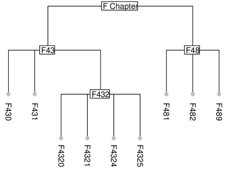
From a statistical perspective, rare features are unlikely to act alone, rather, they tend to impact the outcome in a collective and interactive way. Therefore, properly balancing the rarity and the specificity of the rare features holds the key in harvesting useful information from them. Fortunately, there often exists an inherited or derived hierarchical tree structure among the rare (binary) features, making it possible to perform interpretable rare feature aggregation. Particularly, in EHR data analysis, ICD codes are organized in a hierarchical structure, where the higher-level codes represent more generic disease categories and the lower-level codes represent more specific diseases and conditions. Figure 1 displays an example with ICD-10-CM (International Classification of Diseases, Tenth Revision, Clinical Modification) codes, where each binary feature, as a leaf node in the tree, indicates the absence/presence of a very specific disease condition. The F4320–F4325 codes indicate different types of “adjustment disorder”, which can be collapsed into F432, their parent node; F432 is itself is a sub-category of F43, “reaction to severe stress, and adjustment disorders”. We remark that the ICD-10-CM system is very comprehensive with over 69,000 diagnosis codes; the example here is only a small subset of the F Chapter code set, which is about mental, behavioral and neurodevelopmental disorders. There are other examples: in microbiome studies, the evolutionary history of the taxa is charted through a taxonomic tree with up to seven taxonomic ranks: kingdom, phylum, class, order, family, genus, and species; in text mining and classification, a hierarchical structure of the keywords can be derived and utilized from pre-trained word embeddings such as GloVe and fastText (Naumov et al., 2021).

With the available hierarchical structure, one naive approach of reducing feature rarity (and dimension) is to collapse all the features to a higher level in the hierarchy. Indeed, in EHR applications it is common to use only the first few digits of ICD codes for high-level disease categories, and in microbiome studies it is common to perform the analysis with aggregated data at the genus or order level. Although this simple approach maintains conformity to the tree structure (Cartwright, 2013; Deschepper et al., 2019), it results in indifferent loss of specificity across all feature categories/branches. Some recent works have considered supervised and data-driven rare feature aggregation. She (2010) considered clustered lasso without any side information. Liu and Ye (2010) proposed tree structured group lasso and introduced an efficient algorithm; their method was deployed in Jovanovic et al. (2016) to build a predictive model for hospital readmission based on ICD codes, resulting in a more interpretable model with fewer high-level diagnoses and comparable prediction accuracy. Yan and Bien (2021) proposed a feature aggregation method in high-dimensional regression through a tree-guided equi-sparsity regularization. It has been applied on count data and further specialized to handle compositional data (Li et al., 2022; Liu et al., 2021). However, all the above approaches are designed for numerical features, where the features are aggregated through summation. As such, these methods do not encode any feature interactions or non-linear effects and may not be ideal for handling rare binary features from EHR data.

We propose a novel tree-guided feature selection and logic aggregation (TSLA) approach for large-scale regression with rare binary features, in which dimension reduction is achieved through not only a sparsity pursuit, but also an aggregation promoter with the logic operation of “or”, as guided by any given hierarchical structure of the features. The utilization of the “or” operation is novel yet very natural for binary features, and this distinguishes our work from existing summation-based feature aggregation methods (Yan and Bien, 2021; Liu et al., 2021). Since the “or” operation involves interaction terms between binary features, our approach automatically encodes nonlinear yet interpretable effects of the features on the response. Furthermore, our TSLA approach can be regarded as a tailored logic regression (Ruczinski et al., 2003, 2004; Kooperberg et al., 2001; Schwender and Ickstadt, 2008), which, in its general form, aims to learn Boolean combinations among predictors and is highly non-convex and computationally intensive. In contrast, by formulating the task as a convex linearly-constrained regularized estimation problem, our approach enables efficient and scalable computation. Our logic aggregation approach is appealing in EHR applications; in predictive modeling with ICD diagnosis features, it holds promise to identify the important disease categories and subcategories and simultaneously determine the right levels of specificity in different disease categories.

The rest of the paper is organized as follows. In Section 2, we introduce our logic aggregation framework for binary features in the context of EHR data. Through a tree-guide three-step procedure of feature expansion, model reparameterization, and regularization, we formulate the problem as an equi-sparse regularized regression. In Section 3, a smooth proximal gradient algorithm is introduced for efficient computation and some main theoretical results are discussed. Simulation studies are carried out in Section 4, where both regression and classification scenarios are considered. The suicide risk modeling with EHR data is carried out in Section 5. Some concluding remarks are provided in Section 6. Computational details, theoretical analysis, supporting numerical results, and another application with user-rating data are provided in the Appendix.

2 Logic Aggregation Framework with EHR Data

Let $y\in\mathbb{R}$ be a response/outcome variable and ${\bf x}=(x_{1},\ldots,x_{p_{0}})^{\rm T}{}\in\mathbb{R}^{p_{0}}{}$ be a $p_{0}$-dimensional predictor vector. Suppose $n$ copies of independent data on $(y,{\bf x})$ are available, and denote ${\bf y}=(y_{1},\ldots,y_{n})^{\rm T}{}\in\mathbb{R}^{n}{}$ as the response vector and ${\bf X}_{0}=({\bf x}_{1},\ldots,{\bf x}_{n})^{\rm T}{}\in\mathbb{R}^{n\times p_{0}}{}$ as the predictor matrix.

We are interested in the scenarios in EHR data analysis that the $p_{0}$ features are binary, sparse, high dimensional, and associated with a hierarchical grouping structure. See Figure 1 for an example in EHR data analysis with ICD-10-CM codes. With the given feature hierarchy, there is a trade-off between data resolution/specificity and data sparsity. The main problem we are going to tackle is to efficiently identify the optimal levels of specificity in the feature hierarchy in supervised learning tasks. In the context of EHR data analysis, this amounts to select and identify properly aggregated absence/presence patterns of disease conditions for best predicting an clinical outcome of interest.

The novelty of our approach is to reformulate this combinatorial problem into a convex scalable learning problem through three major steps: (1) feature expansion, (2) reparameterization, and (3) equi-sparsity regularization.

2.1 Tree-guided Feature Expansion

A simple yet critical observation is that under the linear regression setup, the aggregation of two binary features through the “or” operation amounts to require a special linear constraint of the parameters in a regression model that includes their two-way interaction term. Specifically, for two binary features, say, $x_{1}$ and $x_{2}$, we can write

$$x_{1}\ \lor\ x_{2}\ =\, \ x_{1}\ +\ x_{2}\ -\ x_{1}\wedge x_{2}$$

$$=\, \ x_{1}\ +\ x_{2}\ -\ x_{1}x_{2},$$ (1)

where the symbols “$\lor$” and “$\wedge$” denotes the logic “or” and “and” operators, respectively. Therefore, in a linear regression model with $x_{1}$, $x_{2}$ and their two-way interaction $x_{1}x_{2}$, the two predictors can be aggregated if and only if

$$\beta_{1}\ =\ \beta_{2}\ =\ -\beta_{12},$$ (2)

where $\beta_{1}$, $\beta_{2}$, and $\beta_{12}$ are the regression coefficients corresponding to $x_{1}$, $x_{2}$, and $x_{1}x_{2}$, respectively. More generally, the aggregation of multiple binary predictors corresponds to a parameter constraint that involves higher-order interaction terms. For $r$ ($r\geq 2$) binary features, we can write

$$x_{1}\ \lor\ x_{2}\ \lor\ \cdots\ \lor\ x_{r}= \sum_{i=1}^{r}{}\ x_{i}\ -\ \sum_{i\neq j}\ x_{i}x_{j}\ +\ \sum_{i\neq j\neq k}x_{i}x_{j}x_{k}\ +\ \cdots\ +\ (-1)^{r-1}{}\prod_{i=1}^{r}{}x_{i},$$ (3)

and they can be aggregated if and only if their corresponding regression coefficients satisfy

$$\beta_{i}\ =\ -\beta_{ij}\ =\ \beta_{ijk}\ =\ \cdots\ =\ (-1)^{r-1}{}\beta_{12\cdots r}.$$ (4)

The above equivalency reveals that the binary feature aggregation through the “or” operation can be formulated as promoting certain linear constraints of the regression coefficients in a model with both main effects terms and appropriate interaction terms.

Consequently, the first step of our framework is to expand the feature set and the corresponding tree structure by including the interaction terms involved in the possible “or” operations in conformity to the feature hierarchy. On the one hand, the conventional main-effects regression is no longer adequate, as we now need a more comprehensive model with interactions. On the other hand, unlike the fully flexible logic regression, in our framework the possible aggregations are guided and restricted by the hierarchical tree structure. Besides, in practice many high-order interaction terms of the rare features could become zero vectors, so they can be directly dropped from the model. In EHR data, the simultaneous presence of a set of rare and related medical conditions is certainly possible but also is even more rare. So the potential computational burden associated with this tree-guided feature expansion is more bearable than it appears.

To proceed, we introduce some standard terminologies of the tree structure. For a tree ${\bf T}$, let $I({\bf T})$ and $L({\bf T})$ denote the set of internal nodes and the set of leaf nodes, respectively. For a node $u$, denote $C(u)$, $A(u)$ and $D(u)$ as the set of child nodes of $u$, the set of ancestor nodes of $u$, and the set of descendant nodes of $u$, respectively.

In our problem, the original $p_{0}$ nodes and nodes generated for their interactions are referred as “native” nodes and “derived” nodes, respectively. We denote each derived node in the expanded tree as $u_{(\mathcal{S})}^{h}{}$, where the superscript $h$ indicates the depth of the node on the tree, and $\mathcal{S}$, the aggregation set, gives the corresponding nodes at the same height that are involved in the construction of the node. Figure 2(a) provides an illustration of the feature expansion. The original tree is with $p_{0}=5$ leaf nodes and of depth $h=2$. In this example, $u_{j}^{2}{}$, $j=1,\ldots,5$, are the native leaf nodes corresponding to $x_{j}$, $j=1,\ldots,5$. The node $u_{(12)}^{2}{}$ is a derived node from $\mathcal{S}=\{u_{1}^{2}{},u_{2}^{2}{}\}$, which corresponds to the two-way interaction of $x_{1}$ and $x_{2}$. Similarly, the node $u_{(12)}^{1}{}$ is a derived node from $\mathcal{S}=\{u_{1}^{1}{},u_{2}^{1}{}\}$, which corresponds to the interaction of $(x_{1}\lor x_{2}\lor x_{3})$ and $(x_{4}\lor x_{5})$. Under our framework, potential aggregation only happens to the set of features corresponding to the child nodes $C(u)$ of each internal node $u$.

(a) Feature expansion

(b) Reparameterization

Figure 2: Tree-guided feature expansion and reparameterization. Circles and squares indicate native and derived nodes, respectively. For example, on the left panel, node $u_{(12)}^{1}{}$ is derived from $u_{1}^{1}{}$ and $u_{2}^{1}{}$ from their two-way interaction. On the right panel, solid and blank nodes indicate non-zero and zero coefficients, respectively.

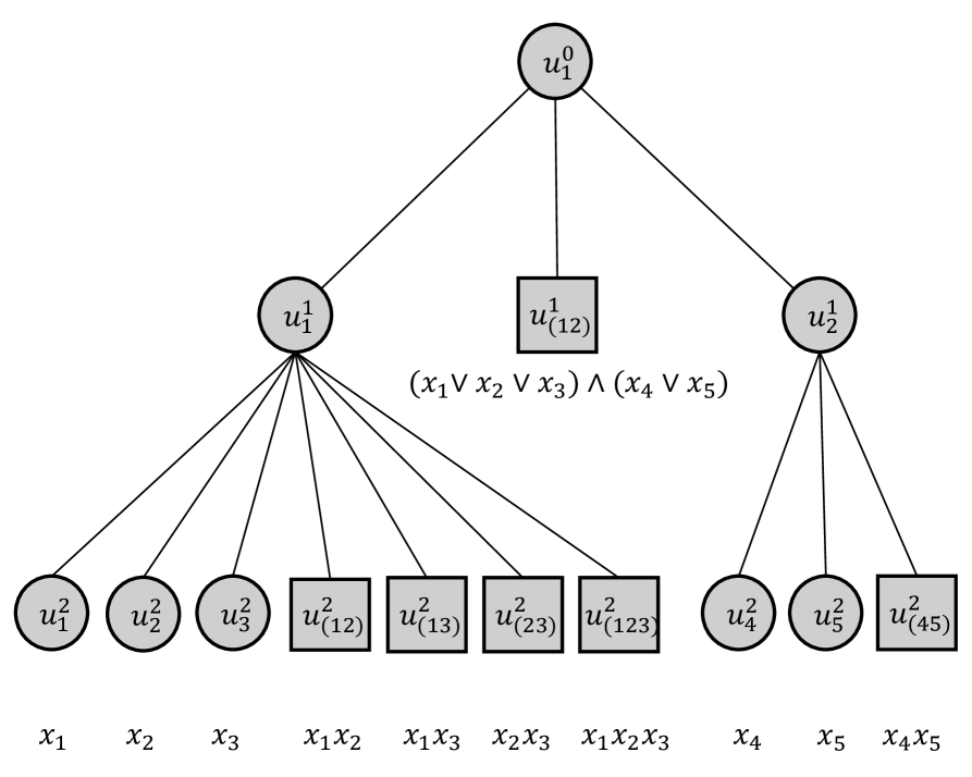
Through the aforedescribed process, the original design matrix ${\bf X}_{0}\in\mathbb{R}^{n\times p_{0}}{}$ is expanded to be the new design matrix ${\bf X}\in\mathbb{R}^{n\times p}{}$, which consists of both the original binary predictors and the generated (non-zero) interaction columns. This enables us to pursue tree-guided binary feature aggregation under the linear regression model

$${\bf y}=\,\mu{\bf 1}\ +\ {\bf X}\mbox{\boldmath$\beta$}\ +\ \mbox{\boldmath$\varepsilon$},$$ (5)

where $\mu\in\mathbb{R}$ is the intercept, ${\bf 1}\in\mathbb{R}^{n}{}$, $\mbox{\boldmath$\beta$}\in\mathbb{R}^{p}{}$ is the regression coefficient vector, and $\mbox{\boldmath$\varepsilon$}\in\mathbb{R}^{n}{}$ is the random error vector. Correspondingly, let ${\bf T}$ be the expanded tree of the feature grouping structure; it is with in total $p$ leaf nodes (among which $p_{0}$ nodes are native) and is of depth $h$.

2.2 Tree-guided Reparameterization

With the expanded linear interaction model in (5), the main problem now is how to parameterize it to facilitate feature aggregation through the “or” operation, i.e., to promote the linear constraints of the form in (2). Motivated by Yan and Bien (2021) and Li et al. (2022), we propose a tree-guided reparametrization of the model in (5).

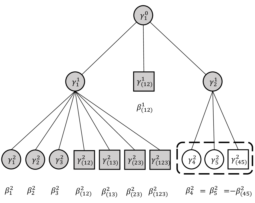
An intermediate coefficient $\gamma_{u}$ is assigned to each node $u$ of the expanded tree ${\bf T}$ with $p_{0}$ native nodes and of depth $h$. For each native leaf node $u_{j}^{l}{}$, for $l=\{0\ldots h\}$, its corresponding regression coefficient, denoted as $\beta_{j}^{l}{}$, is parameterized as

$$\beta_{j}^{l}{}\ =\,\sum_{u\in A(u_{j}^{l}{})\cup\{u_{j}^{l}{}\}}\gamma_{u}.$$ (6)

For each derived leaf node, $u_{(\mathcal{S})}^{l}{}$, for $l=\{0\ldots h\}$, its parameterization is according to the sign of the interaction terms from the potential “or” operations,

$$\beta_{(\mathcal{S})}^{l}{}\ =\ (-1)^{|\mathcal{S}|-1}{}\times\sum_{u\in A(u_{(\mathcal{S})}^{l}{})\cup\{u_{(\mathcal{S})}^{l}{}\}}\gamma_{u},$$ (7)

where $|\mathcal{S}|$ is the cardinality of the aggregation set $\mathcal{S}$.

Through this reparameterization, any potential “or” operation conforming to the tree structure can be expressed as a set of sparsity constraints on the $\gamma_{u}$ coefficients. As shown in Figure 2(b) we have that $\beta_{4}^{2}{}=\ \gamma_{4}^{2}{}+\gamma_{2}^{1}{}+\gamma_{1}^{0}{}$, $\beta_{5}^{2}{}=\ \gamma_{5}^{2}{}+\gamma_{2}^{1}{}+\gamma_{1}^{0}{}$, and $\beta_{(45)}^{2}{}=-\gamma_{(45)}^{2}{}-\gamma_{2}^{1}{}-\gamma_{1}^{0}{}$. Therefore, the aggregation of $x_{4}$ and $x_{5}$ into $x_{4}\lor x_{5}$ is equivalent to $\beta_{4}^{2}{}=\beta_{5}^{2}{}=-\beta_{(45)}^{2}{}$ or $\gamma_{4}^{2}{}=\gamma_{5}^{2}{}=\gamma_{(45)}^{2}{}=0$.

With any given tree ${\bf T}$, denote the number of nodes in ${\bf T}$ as $|{\bf T}|$, let $\mbox{\boldmath$\gamma$}=(\gamma_{u})\in\mathbb{R}^{|{\bf T}|}{}$ be the vector collecting all the intermediate coefficients on the tree. The transformation from $\beta$ to $\gamma$ is linear and deterministic, which can be expressed as $\mbox{\boldmath$\beta$}={\bf A}\mbox{\boldmath$\gamma$}$ with ${\bf A}\in\mathbb{R}^{p\times|{\bf T}|}{}$ derived from the expanded tree structure as (6) and (7).

2.3 Tree-guided Regularization

From the previous discussion, aggregating a set of features under the same ancestor node $u$ is equivalent to setting all intermediate $\gamma$ coefficients in $D(u)$ to be 0. As a consequence, equi-sparsity in $\beta$ can be achieved by inducing zero-sparsity in $\gamma$ coefficients with structured regularization. With a given tree ${\bf T}$, we construct $\mathcal{G}$ as a set of non-overlapped node groups, where

$$\mathcal{G}\ =\ \{u_{1}^{0}{}\}\cup\{C(u),\ u\in I({\bf T})\}.$$ (8)

Then the groups in $\mathcal{G}$ form a partition of nodes in tree ${\bf T}$ and $D(u)$ can be expressed as the union of node groups in $\mathcal{G}$ for all ${\bf u}\in I({\bf T})$. We consider the Child-$\ell_{2}$ (cl2) penalty in $\gamma$ based on the set $\mathcal{G}$, which is constructed as

$$P_{T}(\mbox{\boldmath$\gamma$})=\sum_{g\in\mathcal{G}}w_{g}\|\mbox{\boldmath$\gamma$}_{g}\|,$$ (9)

where $\mbox{\boldmath$\gamma$}_{g}\in\mathbb{R}^{p_{g}}{}$ is a sub-vector of $\gamma$ corresponding to nodes in group $g$ and $p_{g}$ is the size of $g$.

The Child-$\ell_{2}$ penalty is in the form of a typical weighted group-lasso penalty with no overlapping between groups, where the root node is also regularized as a singleton. This is different from the penalties used in Yan and Bien (2021) and Li et al. (2022), where the $\gamma$ coefficient at the root node is always set to be zero. The weight parameter $w_{g}$ for each group can be selected to control relative importance between groups, depending on the specific assumptions of the true tree structure. For all the following numerical studies, we use the group weight suggested in our theoretical results in Section B of the Appendix as

$$w_{g}\ =\ \sqrt{\frac{p_{g}}{2^{k}{}-1}},$$ (10)

where $p_{g}$ is the size of group $g$ and $k$ is the maximum number of child nodes of the original tree before expansion.

Finally, our proposed tree-guided feature selection and logic aggregation (TSLA) approach is expressed as the following optimization problem:

$$(\hat{\mu},\ \hat{}\mbox{\boldmath$\beta$},\ \hat{}\mbox{\boldmath$\gamma$})= \arg\min\{\frac{1}{2n}\|{\bf y}-\mu{\bf 1}-{\bf X}\mbox{\boldmath$\beta$}\|^{2}{}+\lambda[(1-\alpha)\sum_{j}^{p}{}\tilde{w}_{j}|\beta_{j}|+\alpha P_{T}(\mbox{\boldmath$\gamma$})]\},\ \mbox{s.t}\ \mbox{\boldmath$\beta$}\ =\ {\bf A}\mbox{\boldmath$\gamma$},$$ (11)

where $\alpha\in[0,\ 1]$, $\lambda>0$, $\mu\in$ $\mathbb{R}$, $\mbox{\boldmath$\beta$}\in$ $\mathbb{R}^{p}{}$, and $\mbox{\boldmath$\gamma$}\in$ $\mathbb{R}^{|{\bf T}|}{}$. Here, an additional $\ell_{1}$ penalty term of $\beta$ is included to enable feature selection. In our study, we use $\tilde{w}_{j}=\|{\bf x}_{j}\|/\sqrt{n}$ to take into account the scale of each feature. The tuning parameter $\alpha$ controls the balance between selection and aggregation while $\lambda$ controls the overall regularization level.

3 Scalable Computation and Theoretical Guarantee

To solve the optimization problem in (11), we first rewrite it as an unconstrained problem of $\gamma$ and $\mu$ by replacing $\beta$ with ${\bf A}\mbox{\boldmath$\gamma$}$, which gives

$$(\hat{\mu},\ \hat{}\mbox{\boldmath$\gamma$})=\, \arg\min\{\frac{1}{2n}\|{\bf y}-\mu{\bf 1}-{\bf X}{\bf A}\mbox{\boldmath$\gamma$}\|^{2}{}+\lambda(1-\alpha)\|{\bf D}{\bf A}\mbox{\boldmath$\gamma$}\|_{1}+\lambda\alpha P_{T}(\mbox{\boldmath$\gamma$})\},$$ (12)

where ${\bf D}\in\mathbb{R}^{p\times p}{}$ is a diagonal matrix with the $j^{th}{}$ diagonal element as $\tilde{w}_{j}$. This is a convex problem, but the penalty function is non-smooth. We adopt a Smoothing Proximal Gradient (SPG) algorithm (Chen et al., 2012) for the optimization. The algorithm can be readily extended to the settings of logistic regression for binary response, by replacing the $\ell_{2}$ loss with the negative log-likelihood function. For large-scale data, the fast iterative shrinkage-thresholding algorithm (FISTA) (Beck and Teboulle, 2009) is applied in SPG for optimization. The FISTA combines the gradient descent method with the Nesterov acceleration technique (Nesterov, 1983), which leads to faster convergence than standard gradient-based methods. The optimal combination of the tuning parameters $\alpha$ and $\lambda$ can be determined via cross validation. All the details are provided in Section A of the Appendix.

After getting the estimator $\hat{}\mbox{\boldmath$\gamma$}$, the feature aggregation structure can be derived by selecting groups with nonzero coefficients. Due to the “over-selection” property of the convex group lasso penalty (Wei and Huang, 2010), a thresholding operation is preferred in practice to produce a more sparse group structure. Denote $\hat{m}_{g}=w_{g}\|\hat{\mbox{\boldmath$\gamma$}}_{g}\|$. We select group $g$ if

$$\frac{\hat{m}_{g}}{\sum_{g\in\mathcal{G}}\hat{m}_{g}}>\frac{1}{|\mathcal{G}|},$$ (13)

where $w_{g}$ is the weight for group $g$ specified in (10) and $|\mathcal{G}|$ is the cardinality of $\mathcal{G}$.

We have studied the theoretical properties of TSLA under a general high-dimensional framework. Our result reveals that the complexity of the logic aggregation problem depends on the tree structure of the feature hierarchy mainly through the number of original features ($p_{0}$), the height of the tree ($h$), and the maximum number of child nodes ($k$). This is not surprising, as the interactions of each set of child nodes are needed in order to pursue their potential logic aggregation. In the case of a “slim” tree where the maximum number of child nodes is a small value or constant, our framework is expected to show good performance. Moreover, we show that there is a unique coarsest “true aggregation set” corresponding to the true regression coefficient vector $\mbox{\boldmath$\beta$}^{*}{}$. When the true model has both zero-sparsity and equi-sparsity in $\mbox{\boldmath$\beta$}^{*}{}$, the $\ell_{1}$ norm of $\mbox{\boldmath$\beta$}^{*}{}$ then gives a nature measure of the complexity of the true model. Finally, we show that under Gaussian error assumption and with proper choice of the tuning parameters, the following non-asymptotic prediction error bound holds,

$$\frac{1}{n}\|{\bf X}\hat{}\mbox{\boldmath$\beta$}-{\bf X}\mbox{\boldmath$\beta$}^{*}{}\|^{2}{}\preceq\sigma\sqrt{(2^{k}{}-1)}\sqrt{\frac{\log p}{n}}\|\mbox{\boldmath$\beta$}^{*}{}\|_{1},$$

where $\preceq$ means that the inequality holds up to a multiplicative constant, and $\sigma$ is the error standard deviation. It is then clear that the prediction error is controlled by both the structure of the tree ${\bf T}$ and the structure of the underlying coarsest aggregation tree of the true model. The result is consistent with existing works on feature aggregation problems (Yan and Bien, 2021; Li et al., 2022) and can be readily extended to generalized linear models (van de Geer, 2008). All details and proofs are provided in Section B of the Appendix.

4 Simulation

We compare the proposed tree-guided feature selection and logic aggregation (TSLA) approach to several competing methods under both regression and classification settings through simulation. The competing methods include the least squares or logistic regression with the original features (LR), the elastic-net penalized linear or logistic regression with the original features (Enet), the elastic-net penalized linear or logistic regression with both the original features and their two-way interactions (Enet2), and the tree-guided rare feature selection method by Yan and Bien (2021) through the “sum” operation (RFS-Sum). As a benchmark, the oracle linear or logistic regression using the true aggregated features (ORE) is also included. For any regularized method, we use 5-folds cross validation for tuning parameter selection.

Three tree structures of different complexities and dimensions are considered, as shown in Figures 6–8 in Section C.1 of the Appendix. For Tree 1, 2 and 3, the number of original leaf nodes, $p_{0}$, is 15, 42, and 43, respectively, and the number of maximum child nodes, $k$, is 4, 11, and 10, respectively. In each case, the original design matrix ${\bf X}_{0}\in\mathbb{R}^{n\times p_{0}}{}$ is generated as a sparse binary matrix with independent Bernoulli$(0.1)$ entries. Through the feature expansion step in Section 2.1, the new design matrix ${\bf X}\in\mathbb{R}^{n\times p}{}$ is obtained, and its dimension $p$, i.e., the number of non-null leaf nodes of the expanded tree, can reach around 40, 540, and 400 for Tree 1, 2, and 3, respectively.

4.1 Simulation under Regression Settings

Under the regression settings, the continuous response variable $y$ follows the model

$$y\ =\ 2+3(x_{1}\ \lor\ x_{2}\ \lor\ x_{3}\ \lor\ x_{4})-5x_{9}+1.5\{(x_{10}\ \lor\ x_{11}\ \lor\ x_{12})\lor\ x_{13}\}+\varepsilon,$$

where $\varepsilon\sim N(0,\sigma^{2}{})$ with $\sigma^{2}{}$ determined to control the signal to noise ratio (SNR) defined as $\mathrm{var}(\mu{\bf 1}+{\bf X}\mbox{\boldmath$\beta$})/\sigma^{2}{}$. We consider three scenarios,

• Case 1 (low dimensional, low SNR): Tree 1 with $n=200$ and $\mbox{SNR}=0.5$.

• Case 2 (low dimensional, high SNR): Tree 1 with $n=200$ and $\mbox{SNR}=2$.

• Case 3 (high dimensional): Tree 2 with $n=200$ and $\mbox{SNR}=2$.

For each method, the prediction performance is measured by out-of-sample mean squared error (MSE) evaluated on independently generated testing data of sample size 200. The feature aggregation accuracy is measured by false positive rate (FPR) and false negative rate (FNR) in selecting the correct feature grouping pattern. For each setting, the simulation is repeated for 100 times, we report the means and standard errors of the performance metrics.

The results are shown in Table 1. In all cases, the proposed TSLA approach has the best predictive performance. The improvement over other competing methods is more substantial when the model dimension is high and the SNR is low, where proper feature reduction is the most critical. The RFS-Sum method is the second best in prediction, indicating the benefit of utilizing the tree structure as side information. In terms of feature aggregation, TSLA outperforms RFS-Sum and has low FNR and FPR in general. These results show the promise of our proposed framework.

Table 1: Simulation: prediction and feature aggregation performance in regression settings. Reported are the means and standard errors (in parentheses) of the MSE and FNR/FPR over 100 repeated experiments.

	MSE						FNR/FPR
	ORE	TSLA	RFS-Sum	Enet	Enet2	LR	TSLA	RFS-Sum
Case 1	9.75 (1.37)	10.43 (1.50)	10.62 (1.45)	10.76 (1.48)	11.60 (1.65)	10.83 (1.47)	0.12/0.13 (0.22/0.09)	0.31/0.17 (0.25/0.10)
Case 2	2.44 (0.34)	2.66 (0.40)	2.97 (0.39)	3.02 (0.40)	3.31 (0.46)	3.03 (0.40)	0.20/0.05 (0.25/0.08)	0.23/0.09 (0.25/0.09)
Case 3	2.50 (0.37)	3.19 (0.46)	3.22 (0.46)	3.25 (0.47)	3.73 (0.56)	3.66 (0.55)	0.24/0.28 (0.25/0.05)	0.39/0.28 (0.23/0.06)

4.2 Simulation under Classification Settings

The binary response $y$ is generated as $y\sim\mbox{Bernoulli}(q)$, where $q=exp(\eta)/\{1+exp(\eta)\}$, and

$$\eta= -5a+b[z+5(x_{1}\ \lor\ x_{2}\ \lor\ x_{3}\ \lor\ x_{4})+4x_{9}-1.5\{(x_{10}\ \lor\ x_{11}\ \lor\ x_{12})\lor\ x_{13})\}]+$$

$$c(x_{18}\ \lor\ x_{19})-d(x_{20}\ \lor\ x_{21}\ \lor\ x_{22}),\,\mbox{with}\,z\sim N(0,0.25).$$

We consider several scenarios,

• Case 1 (low-dimensional, $q\approx 0.17$): Tree 1 with $n=200$ and $(a,b,c,d)=(1,1,0,0)$.

• Case 2 (low-dimensional, $q\approx 0.17$): Tree 1 with $n=200$ and $(a,b,c,d)=(0.66,0.6,0,0)$.

• Case 3 (low-dimensional, $q\approx 0.30$): Tree 1 with $n=200$ and $(a,b,c,d)=(0.7,1,0,0)$.

• Case 4 (high-dimensional, $q\approx 0.17$): Tree 3 with $n=100$ and $(a,b,c,d)=(0.9,1,1.5,-3.5)$.

For each method, we evaluate out-of-sample classification performance with independently generated testing data of sample size 1000. Besides the area under the curve (AUC) value, we also report the area under the precision-recall curve (AUPRC) value, and the sensitivity and positive predictive value (PPV) under either 90% or 95% specificity; the latter measures are more useful in situations with a rare outcome, as in the suicide risk modeling application to be presented in Section 5. The rest of the setups are the same as in the regression settings.

The results for Case 1 and Case 4 are reported in Table 2 and 3, respectively, and the rest of the results can be founded in Section C.2 of the Appendix. In most of the cases, TSLA leads to higher AUC and AUPRC values than the competing methods. Both TSLA and RFS-Sum perform much better than the other methods. TSLA outperforms RFS-Sum with a large margin in Case 1, and otherwise the improvement is not substantial. We also find that the difference between the methods gets smaller when the response becomes more balanced. This indicates that our method can be more useful with imbalanced data. The other observations are similar as those in the regression settings.

Table 2: Simulation: prediction performance in classification settings under Case 1.

			Sensitivity		PPV
Model	AUC	AUPRC	90% specificity	95% specificity	90% specificity	95% specificity
ORE	0.92 (0.01)	0.71 (0.04)	0.71 (0.06)	0.53 (0.07)	0.59 (0.03)	0.68 (0.04)
TSLA	0.90 (0.02)	0.63 (0.06)	0.62 (0.07)	0.43 (0.07)	0.56 (0.04)	0.63 (0.05)
RFS-Sum	0.88 (0.03)	0.55 (0.05)	0.57 (0.07)	0.37 (0.06)	0.54 (0.04)	0.60 (0.05)
Enet	0.87 (0.02)	0.55 (0.05)	0.55 (0.07)	0.38 (0.06)	0.53 (0.04)	0.60 (0.04)
Enet2	0.84 (0.04)	0.51 (0.05)	0.51 (0.06)	0.32 (0.06)	0.51 (0.04)	0.56 (0.06)
LR	0.84 (0.04)	0.54 (0.05)	0.55 (0.06)	0.36 (0.06)	0.53 (0.04)	0.59 (0.05)

Table 3: Simulation: prediction performance in classification settings under Case 4.

			Sensitivity		PPV
Model	AUC	AUPRC	90% specificity	95% specificity	90% specificity	95% specificity
ORE	0.93 (0.02)	0.76 (0.06)	0.80 (0.07)	0.60 (0.10)	0.64 (0.03)	0.73 (0.04)
TSLA	0.87 (0.03)	0.60 (0.06)	0.63 (0.08)	0.41 (0.08)	0.58 (0.04)	0.64 (0.05)
RFS-Sum	0.88 (0.03)	0.59 (0.06)	0.62 (0.08)	0.40 (0.07)	0.58 (0.04)	0.64 (0.05)
Enet	0.80 (0.06)	0.48 (0.08)	0.46 (0.10)	0.29 (0.08)	0.51 (0.06)	0.56 (0.07)
Enet2	0.69 (0.08)	0.36 (0.09)	0.33 (0.12)	0.21 (0.12)	0.40 (0.09)	0.45 (0.10)
LR	0.71 (0.05)	0.36 (0.06)	0.38 (0.12)	0.14 (0.16)	0.43 (0.06)	0.48 (0.07)

5 Suicide Risk Modeling with EHR data

5.1 Data and Setup

Suicide is a serious public health problem in the U.S. According to the Centers for Disease Control and Prevention (CDC), in 2019, suicide was the tenth leading cause of death in the US. With EHR data, it is of great interest to use medical history of patients, as recorded by ICD codes, to understand and predict the occurrence of future suicide attempt (Barak-Corren et al., 2017; Walsh et al., 2017; Simon et al., 2018; Su et al., 2020). As mentioned above, the common practice of collapsing full-digit ICD codes to fewer digits may lead to substantial information loss. Here, we aim to apply our data-driven feature aggregation approach to determine the right levels of specificity of diagnosis conditions for predicting suicide.

We use a dataset extracted from the Kansas Health Information Network (KHIN), which contains information on inpatient, outpatient, and emergency room encounters for patients in the network from January 1, 2014 to December 31, 2017. Suicide attempts are identified by both the external cause of injury ICD codes and other ICD code combinations that are indicative of suicidal behaviors (Patrick et al., 2010; Chen and Aseltine, 2017). Since the data contain both ICD-9 and ICD-10 codes, we convert the ICD-9 codes to ICD-10 using the public toolkit AHRQ MapIT (https://qualityindicators.ahrq.gov/resources/toolkits) and all the non-unique mappings related to suicide are also checked and validated by our health research team.

In this study, we include all patients who were with at least one diagnosis record or procedure claim during the recruiting window from January 1, 2014 to December 31, 2015 and were between 18 to 64 years of age at the time of the first suicide diagnosis (for patients who had suicide attempt diagnosis) or the last visit (for patients who did not have suicide attempt diagnosis). Patients whose first recorded visit was suicide attempt are excluded due to lack of historical information. The outcome of interest is the occurrence of suicide attempt. The observation window is from the time of the patient’s first non-suicide related record to either seven days before the time of the first suicide attempt or seven days before the last visit. All the records during the observation window are aggregated, and demographic features and binary features of diagnoses are produced.

In the final patient cohort, there are 214,381 patients, among which there are 1107 cases, i.e., patients who had suicide attempt record during the study period. As a proof of concept, we mainly focus on investigating the “F” chapter of the ICD-10 codes, which is about “mental, behavioral and neurodevelopmental disorders”. A pre-screening is done on all the full-digit ICD codes, where codes with larger than 0.01% prevalence are kept. This results in 165 full-digit ICD codes, which can be aggregated to 51 three-digit ICD codes. To deal with the extreme unbalancing of the data, we use a case-control design. To generate a case-control dataset, all cases are included while the controls are randomly drawn with an 1:8 case-control ratio. Therefore, each resulting case-control dataset is with 1107 cases and 8856 controls. Table 4 is a summary table for one such randomly drawn case-control dataset. Note that the cases and the controls exhibit different age distributions, and the prevalence of the ICD codes are much higher in the cases than in the controls, as expected. The detailed prevalence information for each of the three-digit ICD codes in the F chapter is shown in Figure 9 of the Appendix.

Table 4: Suicide risk study: summary statistics for a case-control dataset. All cases are included, while the controls are randomly drawn with 1:8 case-control ratio from the study cohort. Cases are patients who had suicide attempt diagnosis, while controls are patients who did not have suicide attempt diagnosis till the end of the study period.

	Summary Statistics
Variable	Cases ($n$ = 1107)	Controls ($n$ = 8856)
Male ($n$(%))	434 (39.2%)	3365 (38.0%)
Age ($n$(%))
18-25 years old	398 (36.0%)	1423 (16.1%)
26-39 years old	348 (31.4%)	2471 (28.0%)
40-64 years old	361 (32.6%)	4962 (56.0%)
F-code prevalence (%)
Full-digit	0.90%	0.23%
Three-digit	2.90%	0.75%

With the highly sparse and binary ICD features, we compare the proposed logic selection and aggregation framework with several commonly-used modeling strategies. The 165 full-digit F codes can be divided into 10 subgroups based on their first 2 digits, which form 10 sub-tree structures. We apply TSLA to generate aggregated features within each sub-tree structure and fit an elastic-net penalized logistic regression with all the resulting aggregated features. Three competing methods are considered: LR, Enet, and Enet2, which all use the aggregated three-digit ICD codes (and their interactions).

5.2 Prediction Performance

We evaluate the out-of-sample prediction performance of all methods with 10 generated case-control datasets, each with all cases and randomly selected controls. Each dataset is divided into 70% for training and 30% for testing. We use the similar evaluation metrics as in Section 4.2 and average the results from the 10 datasets. Specifically, with each method, we compute out-of-sample AUC and AUPRC, and in addition, we identify either 5% or 10% of the testing patients with the highest risk and evaluate the associated sensitivity and PPV; due to the very low prevalence of the events, these would be roughly similar to consider 5% or 10% specificity. As the model is constructed based on a case-control design, we also report the adjusted PPV values to reflect the expected performance on the whole cohort; see details in Section D of the Appendix.

Table 5: Suicide risk study: prediction performance with ten case-control datasets.

			Sensitivity		PPV		Adjusted-PPV
Model	AUC	AUPRC	10% positive	5% positive	10% positive	5% positive	10% positive	5% positive
LR	75.8% (0.8%)	33.7% (2.2%)	35.4% (1.5%)	21.3% (1.2%)	39.7% (1.8%)	47.2% (2.6%)	2.6% (0.2%)	3.5% (0.4%)
Enet	76.4% (0.7%)	34.8% (2.0%)	35.6% (1.4%)	21.7% (1.1%)	39.8% (1.5%)	48.2% (2.4%)	2.6% (0.2%)	3.6% (0.3%)
Enet2	76.4% (0.9%)	34.3% (2.2%)	35.4% (1.8%)	21.9% (1.3%)	39.4% (1.9%)	48.5% (2.9%)	2.6% (0.2%)	3.7% (0.4%)
TSLA	76.5% (0.8%)	35.3% (2.0%)	36.2% (1.4%)	22.2% (0.9%)	40.3% (1.5%)	49.1% (1.9%)	2.6% (0.2%)	3.7% (0.3%)

Table 5 shows the out-of-sample prediction performance of all methods. The TSLA approach performs the best. Although the improvement in AUC is not large, the aggregated model may have substantially better AUPRC, sensitivity, and PPV measures than the other methods. For example, our method leads to the highest sensitivity, 36.2%, when 10% of patients are determined as at high risk, as comparing to 35.6% from the best competitor. This has important clinical implications: if we were to label 10% of patients as the high risk group of suicide, our model is able to capture 36.2% of patients who are going to attempt suicide.

5.3 Aggregation Patterns of ICD Codes for Suicide Risk

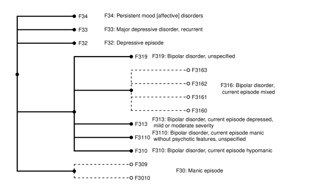
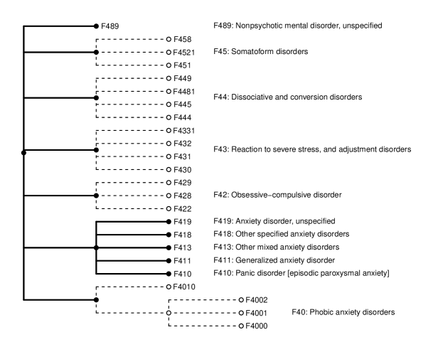
The fitted TSLA model provides valuable insights on the importance and specificity of the F chapter codes to suicide. The results from different case-control datasets are mostly similar, so we report results from one of them (randomly chosen). Figures 3, 4, and 5 show the ICD selection and aggregation patterns of F0, F3, and F4 codes, respectively, and the results for other sub-categories of the F chapter codes are reported in Section D of the Appendix.

Figure 3: Suicide risk study: feature selection and aggregation in F0 codes. The selected codes are indicated by closed circles. The codes that are being aggregated are indicated by open circles and dashed lines.

Figure 4: Suicide risk study: feature selection and aggregation in F3 codes. The settings are the same as in Figure 3.

Figure 5: Suicide risk study: feature selection and aggregation in F4 codes. The settings are the same as in Figure 3.

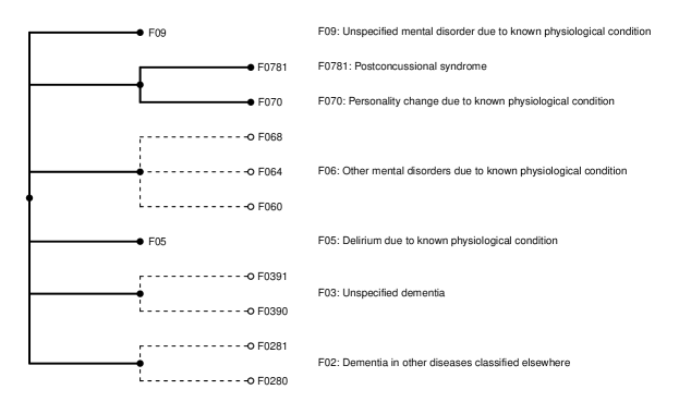
In the category F0 (Mental disorders due to known physiological conditions), F070, which indicates personality change due to known physiological condition, has distinct effect from F0781, which indicates post-concussional syndrome. Indeed, recent systemic studies have shown that patients diagnosed with concussion or mild traumatic brain injury (TBI) had double the risk of suicide when compared with people who did not have brain injuries (Fralick et al., 2019).

In the category of F3 (Mood [affective] disorders), the codes F310, F311, F313, F316 and F319, are suggested to have distinct effects on suicide risk, while all other codes can be aggregated to the three-digit levels. These F31x conditions describe different types of bipolar disorder. For example, F310 and F313 stand for current episode hypomanic and current episode depressed, respectively. These results suggest that the linkage between bipolar disorder and suicide is complicated and distinctive from those between other mental disorders. Recent epidemiological studies have shown that patients with bipolar disorder have a higher risk of committing suicide than patients with other psychiatric or medical disorders; also, it remains unclear whether any bipolar disorder subtype is associated with a higher level of suicidality than the others (Dome et al., 2019; Miller and Black, 2020).

In the category F4 (Anxiety, dissociative, stress-related, somatoform and other nonpsychotic mental disorders), the sub-categories of F41 (Other anxiety disorders) are distinctive, while all other codes can be aggregated to three-digit level. This could be because F410, panic disorder, has a particularly strong association with suicide risk (Nepon et al., 2010). Our analyses also identify some unimportant conditions, e.g., F688 (Other specified disorders of adult personality and behavior) and F641 (Dual role transvestism).

Overall, our results suggest that while a large number of the ICD codes can be aggregated to their first three-digit, there are several important cases where the finer sub-categories should be kept as they show distinct effects on suicide risk. These findings are well supported by current epidemiological studies and meta reviews showing the importance of particular mental health diagnoses in predicting suicide risk.

6 Discussion

In this paper, we develop a novel tree-guided feature selection and logic aggregation framework with the logic operation of “or”, for dealing with sparse, binary features with hierarchical structure from EHR data. By tree-guided feature expansion, reparameterization, and regularization, our approach converts the notoriously difficult combinatorial logic regression problem into a convex learning problem that permits scalable computation. Numerical studies demonstrate that the framework can make productive use of the rare features of diagnosis conditions from EHR data to enhance model prediction and interpretation. The proposed approach is widely applicable; we include another example on user rating prediction with reviews in Section E of the Appendix.

There are many directions for future research. Given that EHR data are often of very large-scale, it is important to explore more scalable computational algorithms or strategies; in particular, it would be promising to develop stagewise estimation techniques (Tibshirani, 2015) for feature aggregation. Our TSLA approach can be extended to other modeling frameworks such as survival analysis, for which the SPG algorithm can still be utilized to handle various combinations of penalty functions and loss functions. Given that EHR data are longitudinal in nature and utilizing longitudinal diagnosis information could lead to better risk identification in suicide risk study, it is pressing to extend our work to longitudinal models. Last but not least, we will explore more general logic operations on rare binary features with a more general graphical association structure.

Appendix

Appendix A Computation

To solve the optimization problem in (11) of the main paper, we first rewrite it as an unconstrained problem of $\gamma$ and $\mu$ by replacing $\beta$ with ${\bf A}\mbox{\boldmath$\gamma$}$, which gives

$$(\hat{\mu},\ \hat{}\mbox{\boldmath$\gamma$})=\, \arg\min\{\frac{1}{2n}\|{\bf y}-\mu{\bf 1}-{\bf X}{\bf A}\mbox{\boldmath$\gamma$}\|^{2}{}+\lambda(1-\alpha)\|{\bf D}{\bf A}\mbox{\boldmath$\gamma$}\|_{1}+\lambda\alpha P_{T}(\mbox{\boldmath$\gamma$})\},$$ (14)

where ${\bf D}\in\mathbb{R}^{p\times p}{}$ is a diagonal matrix with the $j^{th}{}$ diagonal element as $\tilde{w}_{j}$. This is a convex problem, but the penalty function is non-smooth. We thus adopt a Smoothing Proximal Gradient (SPG) algorithm (Chen et al., 2012) for the optimization.

There are three key steps in the SPG algorithm. First, we decouple the penalty terms via dual norms. To be specific, since the $\ell_{1}$ norm is the dual norm of the $\ell_{\infty}$ norm, the second term in (14) can be expressed as

$$\lambda(1-\alpha)\|{\bf D}{\bf A}\mbox{\boldmath$\gamma$}\|_{1}\ =\ \max_{\mbox{\boldmath$\eta$}_{1}\in\mathbb{Q}_{1}}\mbox{\boldmath$\eta$}_{1}^{{}^{\rm T}{}}{}{\bf C}_{1}\mbox{\boldmath$\gamma$},$$

where ${\bf C}_{1}=\lambda(1-\alpha){\bf D}{\bf A}$, $\mbox{\boldmath$\eta$}_{1}\in\mathbb{R}^{p}{}$, and $\mathbb{Q}_{1}=\{\mbox{\boldmath$\eta$}_{1}\mid\|\mbox{\boldmath$\eta$}_{1}\|_{\infty}\leq 1\}$. Similarly, since the dual norm of the $\ell_{2}$ norm is still the $\ell_{2}$ norm, we can write the third term in (14) as

$$\lambda\alpha P_{T}(\mbox{\boldmath$\gamma$})\ =\ \lambda\alpha\sum_{g\in\mathcal{G}}w_{g}\|\mbox{\boldmath$\gamma$}_{g}\|=\ \lambda\alpha\sum_{g\in\mathcal{G}}w_{g}\max_{\|\mbox{\boldmath$\eta$}_{g}\|\leq 1}\mbox{\boldmath$\eta$}_{g}^{{}^{\rm T}{}}{}\mbox{\boldmath$\gamma$}_{g}$$

$$=\ \max_{\mbox{\boldmath$\eta$}_{2}\in\mathbb{Q}_{2}}\sum_{g\in\mathcal{G}}\lambda\alpha w_{g}\mbox{\boldmath$\eta$}_{g}^{{}^{\rm T}{}}{}\mbox{\boldmath$\gamma$}_{g}=\max_{\mbox{\boldmath$\eta$}_{2}\in\mathbb{Q}_{2}}\mbox{\boldmath$\eta$}_{2}^{{}^{\rm T}{}}{}{\bf C}_{2}\mbox{\boldmath$\gamma$},$$

where $\mbox{\boldmath$\eta$}_{g}\in\mathbb{R}^{p_{g}}{}$, $\mbox{\boldmath$\eta$}_{2}$ is a vector of length $\sum_{g\in\mathcal{G}}p_{g}$, collecting all $\mbox{\boldmath$\eta$}_{g}$ for $g\in\mathcal{G}$, and $\mathbb{Q}_{2}=\{\mbox{\boldmath$\eta$}_{2}\mid\|\mbox{\boldmath$\eta$}_{g}\|\leq 1,\ \forall g\in\mathcal{G}\}$. The matrix ${\bf C}_{2}\in\mathbb{R}^{\sum_{g\in\mathcal{G}}p_{g}\times|{\bf T}|}{}$ is defined as follows. The rows of ${\bf C}_{2}$ correspond to each pair of $(u,g)\in\{(u,g)\mid u\in g,\ g\in\mathcal{G},\ u\in{\bf T}\}$ and the columns of ${\bf C}_{2}$ correspond to each node $v\in{\bf T}$. Then each element of ${\bf C}_{2}$ is given by ${{\bf C}_{2}}_{((u,g),v)}=\lambda\alpha w_{g}$ if $u=v$ and ${{\bf C}_{2}}_{((u,g),v)}=0$ otherwise. It then follows that the penalty part in (14) can be expressed as

$$\Omega(\mbox{\boldmath$\gamma$})=\lambda(1-\alpha)\|{\bf D}{\bf A}\mbox{\boldmath$\gamma$}\|_{1}+\lambda\alpha P_{T}(\mbox{\boldmath$\gamma$})\ =\ \max_{\mbox{\boldmath$\eta$}_{1}\in\mathbb{Q}_{1}}\mbox{\boldmath$\eta$}_{1}^{{}^{\rm T}{}}{}{\bf C}_{1}\mbox{\boldmath$\gamma$}+\max_{\mbox{\boldmath$\eta$}_{2}\in\mathbb{Q}_{2}}\mbox{\boldmath$\eta$}_{2}^{{}^{\rm T}{}}{}{\bf C}_{2}\mbox{\boldmath$\gamma$}.$$ (15)

In the second step, by using a smoothing technique proposed in Nesterov (2005), we obtain a smooth approximation of $\Omega(\mbox{\boldmath$\gamma$})$ as

$$f_{\tau}(\mbox{\boldmath$\gamma$})\ =\ \max_{\mbox{\boldmath$\eta$}_{1}\in\mathbb{Q}_{1}}(\mbox{\boldmath$\eta$}_{1}^{{}^{\rm T}{}}{}{\bf C}_{1}\mbox{\boldmath$\gamma$}-\frac{\tau}{2}\|\mbox{\boldmath$\eta$}_{1}\|^{2}{})+\max_{\mbox{\boldmath$\eta$}_{2}\in\mathbb{Q}_{2}}(\mbox{\boldmath$\eta$}_{2}^{{}^{\rm T}{}}{}{\bf C}_{2}\mbox{\boldmath$\gamma$}-\frac{\tau}{2}\|\mbox{\boldmath$\eta$}_{2}\|^{2}{}),$$ (16)

with $\tau$ being the positive smoothness parameter. Then $f_{\tau}(\mbox{\boldmath$\gamma$})$ is smooth with respect to $\gamma$ and the Lipschitz continuous gradient is given as ${\bf C}_{1}^{{}^{\rm T}{}}{}\mbox{\boldmath$\eta$}_{1}^{*}{}+{\bf C}_{2}^{{}^{\rm T}{}}{}\mbox{\boldmath$\eta$}_{2}^{*}{}$, where $(\mbox{\boldmath$\eta$}_{1}^{*}{},\mbox{\boldmath$\eta$}_{2}^{*}{})$ is the optimal solution of (16). The Lipschitz constant is $L_{\tau}=\|{\bf C}_{1}\|^{2}{}/\tau+\|{\bf C}_{2}\|^{2}{}/\tau$, where $\|{\bf C}_{1}\|$ and $\|{\bf C}_{2}\|$ are the matrix spectral norms. As we use a combination of group lasso penalty and generalized lasso penalty, $\mbox{\boldmath$\eta$}_{1}^{*}{}$ and $\mbox{\boldmath$\eta$}_{2}^{*}{}$ have closed-form expressions, and the Lipchitz constant is explicit (Chen et al., 2012). By substituting $\Omega(\mbox{\boldmath$\gamma$})$ in (14) with its smooth approximation $f_{\tau}({\mbox{\boldmath$\gamma$}})$, we obtain the approximated optimization problem

$$(\hat{\mu},\ \hat{}\mbox{\boldmath$\gamma$})\ =\ \arg\min h(\mu,\ \mbox{\boldmath$\gamma$})\ =\ \arg\min\{\frac{1}{2n}\|{\bf y}-\mu{\bf 1}-{\bf X}{\bf A}\mbox{\boldmath$\gamma$}\|^{2}{}+f_{\tau}(\mbox{\boldmath$\gamma$})\}.$$ (17)

The gradient of $h$ with respect to $\mu$ and $\gamma$ is straightforward with explicit Lipschitz constant.

Finally, we perform optimization based on the approximated problem (17), which is convex and smooth. For large scale data, the fast iterative shrinkage-thresholding algorithm (FISTA) (Beck and Teboulle, 2009) is applied in SPG for optimization. The FISTA combines the gradient descent method with the Nesterov acceleration technique (Nesterov, 1983), which leads to faster convergence than standard gradient-based methods.

Let $t$ be the index of the $t^{th}{}$ iteration, and denote $\mu^{(0)}{}$ and $\mbox{\boldmath$\gamma$}^{(0)}{}$ as the initial values of the coefficients. Following the discussion above, the optimization steps for problem (17) can be summarised in Algorithm 1. In our numerical studies, we take $\mu^{(0)}{}=0$ and $\mbox{\boldmath$\gamma$}^{(0)}{}={\bf 0}$.

Input: ${\bf X}$, ${\bf y}$, ${\bf C}_{1}$, ${\bf C}_{2}$, ${\bf A}$, $L$, $\tau$, $\mu^{(0)}{}$, $\mbox{\boldmath$\gamma$}^{(0)}{}$

Initialization: $\theta^{(0)}{}=1$, $w_{1}^{(0)}{}=\mu^{(0)}{}$, ${\bf w}_{2}^{(0)}{}=\mbox{\boldmath$\gamma$}^{(0)}{}$

Repeat1. Compute ${\mbox{\boldmath$\eta$}_{1}^{*}{}}^{(t)}{}$ and ${\mbox{\boldmath$\eta$}_{2}^{*}{}}^{(t)}{}$ with $\mbox{\boldmath$\gamma$}^{(t)}{}$, ${\bf C}_{1}$, ${\bf C}_{2}$ and $\tau$. 2. Get the gradient $\nabla h(w_{1}^{(t)}{})$ and $\nabla h({\bf w}_{2}^{(t)}{})$ with $\nabla h(w_{1}^{(t)}{})=-\frac{1}{n}{\bf 1}^{{}^{\rm T}{}}{}({\bf y}-w_{1}^{(t)}{}{\bf 1}-{\bf X}{\bf A}{\bf w}_{2}^{(t)}{})$, $\nabla h({\bf w}_{2}^{(t)}{})=-\frac{1}{n}({\bf X}{\bf A})^{{}^{\rm T}{}}{}({\bf y}-w_{1}^{(t)}{}{\bf 1}-{\bf X}{\bf A}{\bf w}_{2}^{(t)}{})+{\bf C}_{1}^{{}^{\rm T}{}}{}{\mbox{\boldmath$\eta$}_{1}^{*}{}}^{(t)}{}+{\bf C}_{2}^{{}^{\rm T}{}}{}{\mbox{\boldmath$\eta$}_{2}^{*}{}}^{(t)}{}$. 3. Update the current estimations by $\mu^{(t+1)}{}=w_{1}^{(t)}{}-\frac{1}{L}\nabla h({w_{1}}^{(t)}{})$, $\mbox{\boldmath$\gamma$}^{(t+1)}{}={\bf w}_{2}^{(t)}{}-\frac{1}{L}\nabla h({\bf w}_{2}^{(t)}{})$. 4. Set $\theta^{(t+1)}{}=\frac{1+\sqrt{1+4(\theta^{(t)}{})^{2}{}}}{2}$. 5. Set $w_{1}^{(t+1)}{}=\mu^{(t+1)}{}+\frac{\theta^{(t)}{}-1}{\theta^{(t+1)}{}}(\mu^{(t+1)}{}-\mu^{(t)}{})$, ${\bf w}_{2}^{(t+1)}{}=\mbox{\boldmath$\gamma$}^{(t+1)}{}+\frac{\theta^{(t)}{}-1}{\theta^{(t+1)}{}}(\mbox{\boldmath$\gamma$}^{(t+1)}{}-\mbox{\boldmath$\gamma$}^{(t)}{})$.

Until convergence $(|\mu^{(t)}{}-\mu^{(t-1)}{}|+\|\mbox{\boldmath$\gamma$}^{(t)}{}-\mbox{\boldmath$\gamma$}^{(t-1)}{}\|_{1})/(|\mu^{(t-1)}{}|+\|\mbox{\boldmath$\gamma$}^{(t-1)}{}\|_{1})\leq\ 10^{-5}{}$.

Output: $\mu^{(t)}{}$ and $\mbox{\boldmath$\gamma$}^{(t)}{}$ at convergence

Algorithm 1 Fast Iterative Shrinkage-Thresholding Algorithm for TSLA

The optimal combination of the tuning parameters $\alpha$ and $\lambda$ can be determined via cross validation. The range of $\alpha$ is set as $[0,\ 1]$. For $\lambda$, we compute an approximated upper bound $\lambda^{*}{}$ and take the range as $(0,\ \lambda^{*}{})$.More specifically, for the tuning parameter $\lambda$, we compute an upper bound $\lambda^{*}{}$ with

$$\lambda^{*}{}=\max\{\lambda_{1}^{*}{},\ \lambda_{2}^{*}{}\},\ \lambda_{1}^{*}{}=\max_{1\leq j\leq p}\frac{|{\bf x}_{j}^{{}^{\rm T}{}}{}{\bf y}|}{n\tilde{w}_{j}},\ \lambda_{2}^{*}{}=\max_{g\in\mathcal{G}}\frac{\|{\bf X}_{g}^{{}^{\rm T}{}}{}{\bf y}\|}{nw_{g}},$$ (18)

where ${\bf X}_{g}={\bf X}{\bf A}{\bf P}_{g}$. The weights $\tilde{w}_{j}$ and $w_{g}$ are specified in Section 2.3 of the main paper and ${\bf P}_{g}$ is defined in Section B of the Appendix. Note that, $\lambda_{1}^{*}{}$ is the smallest value for which all the $\beta$ coefficients are zero when $\alpha=0$ and $\lambda_{2}^{*}{}$ is the smallest value for which all the $\gamma$ coefficients are zero when $\alpha=1$. This bound works well in practice. The smoothness parameter $\tau$ controls the gap between $\Omega(\mbox{\boldmath$\gamma$})$ and $f_{\tau}(\mbox{\boldmath$\gamma$})$. In practice, for large scale problems, setting $\tau$ as a small positive value can provide reasonably good approximation accuracy (Chen et al., 2012). We thus set $\tau$ as $10^{-3}{}$ in all numerical studies.

The algorithm can be readily extended to the settings of logistic regression when $y$ is an binary response. The objective function for logistic regression under the aggregation framework can be derived by substituting the first term in (14) with the negative log-likelihood function:

$$\sum_{i=1}^{n}{}[-w_{1}y_{i}\log\mu_{i}-w_{0}(1-y_{i})\log(1-\mu_{i})],\qquad\mu_{i}=\frac{e^{\mu+{\bf x}_{i}^{{}^{\rm T}{}}{}{\bf A}\mbox{\boldmath$\gamma$}}{}}{1+e^{\mu+{\bf x}_{i}^{{}^{\rm T}{}}{}{\bf A}\mbox{\boldmath$\gamma$}}{}},$$

where $w_{1}$ and $w_{0}$ are the weights of positive and negative cases, accordingly. Since the negative log-likelihood function is convex and smooth, the application of SPG is straightforward.

Appendix B Theory

B.1 Theoretical Results

In this section, we study the theoretical properties of the estimator from the proposed TSLA approach under a general high-dimensional learning framework. We consider the regression model without the intercept term

$${\bf y}={\bf X}\mbox{\boldmath$\beta$}+\mbox{\boldmath$\varepsilon$},$$ (19)

where ${\bf X}$ is the expanded binary matrix. As all the binary features are rare, we assume that there is a baseline group of observations for which the feature vector is a zero vector. The intercept then represents the group mean for these baseline observations. Without loss of generality, we assume that the response ${\bf y}$ in (19) has been centered by the baseline mean. Then the intercept term can be excluded from the model.

Under the TSLA framework, we investigate the finite sample properties of the regularized estimator:

$$(\hat{}\mbox{\boldmath$\beta$},\ \hat{}\mbox{\boldmath$\gamma$})=\, \arg\min\{\frac{1}{2n}\|{\bf y}-{\bf X}\mbox{\boldmath$\beta$}\|^{2}{}+\lambda[(1-\alpha)\sum_{j}^{p}{}\tilde{w}_{j}|\beta_{j}|+\alpha P_{T}(\mbox{\boldmath$\gamma$})]\},\ \mbox{s.t}\ \mbox{\boldmath$\beta$}\ =\ {\bf A}\mbox{\boldmath$\gamma$}.$$ (20)

We begin with a discussion on the complexity of the given tree structure.

• A k-ary tree is a rooted tree where every internal node has at most $k$ child nodes.

For a given original tree as a k-ary tree of height $h$, the expanded tree ${\bf T}$ is at most a ($2^{k}{}-1$)-ary tree of the same height. Under TSLA, the dimension of $\beta$, $p$, is the same as the number of leaf nodes in ${\bf T}$. Based on the property of a k-ary tree, it always holds that $p\leq(2^{k}{}-1)^{h}{}$. Assume that the original tree is a k-ary tree of height $h$, our main result is stated in Theorem B.1.

Theorem B.1

Assume that $\mbox{\boldmath$\varepsilon$}\sim N_{n}({\bf 0},\sigma^{2}{}{\bf I}_{n})$. Suppose $(\hat{}\mbox{\boldmath$\beta$},\ \hat{}\mbox{\boldmath$\gamma$})$ is a solution to the optimization problem (20). If we take $\lambda\geq 4\sqrt{2^{k}{}-1}\sigma\sqrt{\frac{\log p}{n}}$, $\tilde{w}_{j}=\|{\bf x}_{j}\|/\sqrt{n}$ for $1\leq j\leq p$ and $w_{g}=\sqrt{\frac{p_{g}}{2^{k}{}-1}}$ for $g\in\mathcal{G}$, then with probability at least $1-\frac{1}{p}-\frac{2}{p^{2}{}}$, it holds that

$$\frac{1}{n}\|{\bf X}\hat{}\mbox{\boldmath$\beta$}-{\bf X}\mbox{\boldmath$\beta$}^{*}{}\|^{2}{}\preceq\lambda((1-\alpha)\sum_{j=1}^{p}{}\tilde{w}_{j}|\beta_{j}^{*}{}|+\alpha P_{T}(\mbox{\boldmath$\gamma$}^{*}{})),$$ (21)

where $\mbox{\boldmath$\beta$}^{*}{}$ and $\mbox{\boldmath$\gamma$}^{*}{}$ are the true coefficients.

Not surprisingly, the result reveals that the model complexity depends on the structure of the original tree, mainly through the number of features, the height of the tree, and the maximum number of child nodes. In the case of a “slim” tree where the maximum number of child nodes is a relatively small value, this framework is expected to show good performance in prediction.

To further study the magnitude of the error bound in Theorem B.1, we introduce the next definition and Lemma B.2 following the discussion in Yan and Bien (2021).

• Denote $V({\bf T})$ as the set of nodes in tree ${\bf T}$. The set of nodes $\mathcal{B}\subseteq V({\bf T})$ is an aggregation set with respect to tree ${\bf T}$ if $\{L(u):u\in\mathcal{B}\}$ forms a partition of $L({\bf T})$.

Lemma B.2

For any $\mbox{\boldmath$\beta$}^{*}{}\in\mathbb{R}^{p}{}$, there exists a unique coarsest aggregation set $\mathcal{B}^{*}{}$ with respect to tree ${\bf T}$ such that (a) $\beta_{j}^{*}{}=\beta_{k}^{*}{}$ for $j,k\in L(u),\ \forall u\in\mathcal{B}^{*}{}$, (b) $|\beta_{j}^{*}{}-\beta_{k}^{*}{}|>0$, $j\in L(u)$ and $k\in L(v)$ for siblings $u,v\in\mathcal{B}^{*}{}$.

Lemma B.2 indicates that there is a unique coarsest “true aggregation set” $\mathcal{B}^{*}{}$ corresponding to the true model coefficient $\mbox{\boldmath$\beta$}^{*}{}$. When the true model has both zero-sparsity and equi-sparsity in $\mbox{\boldmath$\beta$}^{*}{}$, the $\ell_{1}$ norm of $\mbox{\boldmath$\beta$}^{*}{}$ is a nature measure of the model complexity, which is stated in the next corollary.

Corollary B.3

By taking $\lambda\geq 4\sqrt{2^{k}{}-1}\sigma\sqrt{\frac{\log p}{n}}$ and using the weights in Theorem B.1, it can be shown that

$$\frac{1}{n}\|{\bf X}\hat{}\mbox{\boldmath$\beta$}-{\bf X}\mbox{\boldmath$\beta$}^{*}{}\|^{2}{}\preceq\sigma\sqrt{(2^{k}{}-1)}\sqrt{\frac{\log p}{n}}\|\mbox{\boldmath$\beta$}^{*}{}\|_{1},$$ (22)

where $\mbox{\boldmath$\beta$}^{*}{}$ is the true model coefficient vector.

It is then clear that the prediction error is controlled by both the structure of the given tree ${\bf T}$ and the structure of the underlying coarsest aggregation tree.

B.2 Proofs of Theoretical Results

B.2.1 Proof of Theorem B.1

Denote $\Omega(\mbox{\boldmath$\beta$},\ \mbox{\boldmath$\gamma$})=(1-\alpha)P_{T}(\mbox{\boldmath$\beta$})+\alpha P_{T}(\mbox{\boldmath$\gamma$})$ as the penalty function in problem (20) in Section B, where $P_{T}(\mbox{\boldmath$\beta$})=\sum_{j=1}^{p}{}\tilde{w}_{j}|\beta_{j}|$ and $P_{T}(\mbox{\boldmath$\gamma$})=\sum_{g\in\mathcal{G}}w_{g}\|\mbox{\boldmath$\gamma$}_{g}\|$. Here, we take weights $\tilde{w}_{j}=\|{\bf x}_{j}\|/\sqrt{n}$ and $w_{g}=\sqrt{\frac{p_{g}}{2^{k}{}-1}}$, where $p_{g}$ is the number of elements in group $g$, ${\bf x}_{j}$ is the $j^{th}{}$ column of ${\bf X}$, and $k$ is the maximum number of child nodes in the original tree. Let $(\hat{\mbox{\boldmath$\beta$}},\ \hat{\mbox{\boldmath$\gamma$}})$ be a solution to the problem (20), we have

$$\frac{1}{2n}\|{\bf y}-{\bf X}\hat{}\mbox{\boldmath$\beta$}\|^{2}{}+\lambda\Omega(\hat{}\mbox{\boldmath$\beta$},\hat{}\mbox{\boldmath$\gamma$})\ \leq\ \frac{1}{2n}\|{\bf y}-{\bf X}\mbox{\boldmath$\beta$}\|^{2}{}+\lambda\Omega(\mbox{\boldmath$\beta$},\mbox{\boldmath$\gamma$}),$$

for any $(\mbox{\boldmath$\beta$},\ \mbox{\boldmath$\gamma$})$ such that $\mbox{\boldmath$\beta$}={\bf A}\mbox{\boldmath$\gamma$}$. Assume ($\mbox{\boldmath$\beta$}^{*}{},\ \mbox{\boldmath$\gamma$}^{*}{}$) are the true coefficient vectors. Let $\hat{\Delta}^{\gamma}{}=\hat{}\mbox{\boldmath$\gamma$}-\mbox{\boldmath$\gamma$}^{*}{}$ and $\hat{\Delta}^{\beta}{}=\hat{}\mbox{\boldmath$\beta$}-\mbox{\boldmath$\beta$}^{*}{}$. By plugging in ${\bf y}={\bf X}\mbox{\boldmath$\beta$}^{*}{}+\mbox{\boldmath$\varepsilon$}$ and $(\mbox{\boldmath$\beta$},\ \mbox{\boldmath$\gamma$})=(\mbox{\boldmath$\beta$}^{*}{},\ \mbox{\boldmath$\gamma$}^{*}{})$, with some algebra, we have

$$\frac{1}{2n}\|{\bf X}\hat{}\mbox{\boldmath$\beta$}-{\bf X}\mbox{\boldmath$\beta$}^{*}{}\|^{2}{}+\lambda\Omega(\hat{}\mbox{\boldmath$\beta$},\hat{}\mbox{\boldmath$\gamma$})\ \leq\ \lambda\Omega(\mbox{\boldmath$\beta$}^{*}{},\mbox{\boldmath$\gamma$}^{*}{})+\frac{1}{n}\mbox{\boldmath$\varepsilon$}^{{}^{\rm T}{}}{}{\bf X}\hat{\Delta}^{\beta}{}.$$ (23)

For each group $g\in\mathcal{G}$, define ${\bf P}_{g}\in\mathbb{R}^{|{\bf T}|\times|{\bf T}|}{}$ as a diagonal matrix. The diagonal elements of ${\bf P}_{g}$ are given by

$$({\bf P}_{g})_{vv}=\begin{cases}1,&\mbox{if node}\ v\in g;\\ 0,&\mbox{otherwise}.\end{cases}$$

Then the Child-$\ell_{2}$ penalty $P_{T}(\mbox{\boldmath$\gamma$})$ can be re-expressed as

$$P_{T}(\mbox{\boldmath$\gamma$})=\sum_{g\in\mathcal{G}}w_{g}\|\mbox{\boldmath$\gamma$}_{g}\|=\sum_{g\in\mathcal{G}}w_{g}\|{\bf P}_{g}\mbox{\boldmath$\gamma$}\|.$$

Based on the structure of matrix ${\bf P}_{g}$, we also have the following identity:

$$\sum_{g\in\mathcal{G}}{\bf P}_{g}{\bf P}_{g}={\bf I}_{|{\bf T}|}.$$

Recall that from the tree-guided reparameterization, we have $\mbox{\boldmath$\beta$}^{*}{}={\bf A}\mbox{\boldmath$\gamma$}^{*}{}$ and $\hat{\mbox{\boldmath$\beta$}}={\bf A}\hat{\mbox{\boldmath$\gamma$}}$. Consider the second term on the RHS of (23), we have

$$|\frac{1}{n}\mbox{\boldmath$\varepsilon$}^{{}^{\rm T}{}}{}{\bf X}\hat{\Delta}^{\beta}{}| =|(1-\alpha)\frac{1}{n}\mbox{\boldmath$\varepsilon$}^{{}^{\rm T}{}}{}{\bf X}\hat{\Delta}^{\beta}{}+\alpha\frac{1}{n}\mbox{\boldmath$\varepsilon$}^{{}^{\rm T}{}}{}{\bf X}{\bf A}\hat{\Delta}^{\gamma}{}|$$

$$\leq|(1-\alpha)\frac{1}{n}\mbox{\boldmath$\varepsilon$}^{{}^{\rm T}{}}{}{\bf X}\hat{\Delta}^{\beta}{}|+|\alpha\frac{1}{n}\mbox{\boldmath$\varepsilon$}^{{}^{\rm T}{}}{}{\bf X}{\bf A}\hat{\Delta}^{\gamma}{}|.$$ (24)

For the first part on the RHS of (24), let $v_{j}=n^{-1/2}{}{\bf x}_{j}^{{}^{\rm T}{}}{}\mbox{\boldmath$\varepsilon$}$ and $\tilde{w}_{j}=\|{\bf x}_{j}\|/\sqrt{n}$, for $j=1,\ldots,p$, we have

$$|\frac{1}{n}\mbox{\boldmath$\varepsilon$}^{{}^{\rm T}{}}{}{\bf X}\hat{\Delta}^{\beta}{}| =|\sum_{j=1}^{p}{}\frac{{\bf x}_{j}^{{}^{\rm T}{}}{}\mbox{\boldmath$\varepsilon$}}{\sqrt{n}\|{\bf x}_{j}\|}\times\frac{\|{\bf x}_{j}\|}{\sqrt{n}}\hat{\Delta}_{j}^{\beta}{}|$$

$$=|\sum_{j=1}^{p}{}\frac{v_{j}}{\|{\bf x}_{j}\|}\tilde{w}_{j}\hat{\Delta}_{j}^{\beta}{}|$$

$$\leq\max_{1\leq j\leq p}\frac{|v_{j}|}{\|{\bf x}_{j}\|}(\sum_{j=1}^{p}{}\tilde{w}_{j}|\hat{\Delta}_{j}^{\beta}{}|)$$

$$\leq\max_{1\leq j\leq p}\frac{|v_{j}|}{\|{\bf x}_{j}\|}(\sum_{j=1}^{p}{}\tilde{w}_{j}|\hat{\beta}_{j}|+\tilde{w}_{j}|\beta_{j}^{*}{}|)$$

$$=\max_{1\leq j\leq p}\frac{|v_{j}|}{\|{\bf x}_{j}\|}(P_{T}(\mbox{\boldmath$\beta$}^{*}{})+P_{T}(\hat{}\mbox{\boldmath$\beta$})).$$

Since $\mbox{\boldmath$\varepsilon$}\sim N_{n}({\bf 0},\sigma^{2}{}{\bf I}_{n})$, $v_{j}\sim N(0,\sigma^{2}{}\|{\bf x}_{j}\|^{2}{}/n)$ for $j=1,\ldots,p$. By Lemma 6.2 of Bühlmann and Van De Geer (2011), for $t>0$, it holds that

$$P\left(\max_{1\leq j\leq p}\frac{|v_{j}|}{\|{\bf x}_{j}\|}>\sigma\sqrt{\frac{2(t+\log p)}{n}}\ \right)\ \leq\ 2e^{-t}{}.$$

Take $t=2\log p>0$, we get

$$P\left(\ \max_{1\leq j\leq p}\frac{|v_{j}|}{\|{\bf x}_{j}\|}>\sigma\sqrt{\frac{6\log p}{n}}\ \right)\ \leq\ \frac{2}{p^{2}{}}\ .$$ (25)

For the second part on the RHS of (24), using the property of the matrix ${\bf P}_{g}$, we get

$$|\frac{1}{n}\mbox{\boldmath$\varepsilon$}^{{}^{\rm T}{}}{}{\bf X}{\bf A}\hat{\Delta}^{\gamma}{}| =|\frac{1}{n}\mbox{\boldmath$\varepsilon$}^{{}^{\rm T}{}}{}{\bf X}{\bf A}(\sum_{g\in\mathcal{G}}{\bf P}_{g}{\bf P}_{g})\hat{\Delta}^{\gamma}{}|$$

$$=|\frac{1}{n}\sum_{g\in\mathcal{G}}(\mbox{\boldmath$\varepsilon$}^{{}^{\rm T}{}}{}{\bf X}{\bf A}{\bf P}_{g})({\bf P}_{g}\hat{\Delta}^{\gamma}{})|$$

$$\leq\frac{1}{n}\sum_{g\in\mathcal{G}}\sqrt{\frac{2^{k}{}-1}{p_{g}}}\|\mbox{\boldmath$\varepsilon$}^{{}^{\rm T}{}}{}{\bf X}{\bf A}{\bf P}_{g}\|\times\sqrt{\frac{p_{g}}{2^{k}{}-1}}\|{\bf P}_{g}\hat{\Delta}^{\gamma}{}\|$$

$$\leq\max_{g\in\mathcal{G}}\{\frac{1}{n}\sqrt{\frac{2^{k}{}-1}{p_{g}}}\|\mbox{\boldmath$\varepsilon$}^{{}^{\rm T}{}}{}{\bf X}{\bf A}{\bf P}_{g}\|\}\sum_{g\in\mathcal{G}}\sqrt{\frac{p_{g}}{2^{k}{}-1}}\|{\bf P}_{g}\hat{\Delta}^{\gamma}{}\|$$

$$\leq\max_{g\in\mathcal{G}}\{\frac{1}{n}\sqrt{\frac{2^{k}{}-1}{p_{g}}}\|\mbox{\boldmath$\varepsilon$}^{{}^{\rm T}{}}{}{\bf X}{\bf A}{\bf P}_{g}\|\}(\sum_{g\in\mathcal{G}}\sqrt{\frac{p_{g}}{2^{k}{}-1}}\|{\bf P}_{g}\gamma^{*}{}\|+\sum_{g\in\mathcal{G}}\sqrt{\frac{p_{g}}{2^{k}{}-1}}\|{\bf P}_{g}\hat{\gamma}\|)$$

$$=\max_{g\in\mathcal{G}}\{\frac{1}{n}\sqrt{\frac{2^{k}{}-1}{p_{g}}}\|\mbox{\boldmath$\varepsilon$}^{{}^{\rm T}{}}{}{\bf X}{\bf A}{\bf P}_{g}\|\}(P_{T}(\mbox{\boldmath$\gamma$}^{*}{})+P_{T}(\hat{}\mbox{\boldmath$\gamma$})).$$

To bound this second part, we use the following Lemma from Hsu et al. (2012).

Lemma B.4

Let ${\bf Z}$ be an $m\times n$ matrix and let $\mbox{\boldmath$\Sigma$}_{z}={\bf Z}^{{}^{\rm T}{}}{}{\bf Z}$. Suppose $\mbox{\boldmath$\varepsilon$}\sim\ N_{n}({\bf 0},\sigma^{2}{}{\bf I}_{n})$. For all $t>0$,

$$P\left(\ \|{\bf Z}\mbox{\boldmath$\varepsilon$}\|^{2}{}>\sigma^{2}{}(\,\mathrm{tr}(\mbox{\boldmath$\Sigma$}_{z})+2\sqrt{\mathrm{tr}(\mbox{\boldmath$\Sigma$}_{z}^{2}{})t}+2\|\mbox{\boldmath$\Sigma$}_{z}\|t\,)\ \right)\ <\ e^{-t}{},$$

where $\|\mbox{\boldmath$\Sigma$}\|$ denotes the matrix spectral norm.

For each $g\in\mathcal{G}$, denote ${\bf X}_{g}={\bf X}{\bf A}{\bf P}_{g}\in\mathbb{R}^{n\times|{\bf T}|}{}$, and take $\mbox{\boldmath$\Sigma$}_{g}={\bf X}_{g}{\bf X}_{g}^{{}^{\rm T}{}}{}$. It is not hard to see that each column of ${\bf X}_{g}$ is given by aggregating columns in ${\bf X}$ via the “or” operation. Then the element in ${\bf X}_{g}$ is either 0 or 1. For example, in Figure 2 of the main paper, when $u=u_{1}^{0}{}$ and $g=\{u_{1}^{1}{},u_{2}^{1}{},u_{(12)}^{1}{}\}$, the ${\bf X}_{g}$ matrix may have three nonzero columns, which are constructed with $x_{1}\ \lor\ x_{2}\ \lor\ x_{3}$, $x_{4}\ \lor\ x_{5}$, and $(x_{1}\ \lor\ x_{2}\ \lor\ x_{3})\ \wedge\ (x_{4}\ \lor\ x_{5})$, respectively. In fact, the ${\bf X}_{g}$ matrix always has at most $p_{g}$ nonzero columns. Denote ${\bf X}_{g}$ as ${\bf X}_{g}=\{x_{ij}^{g}{}\}_{n\times|{\bf T}|}$, it follows that

$$\mathrm{tr}(\mbox{\boldmath$\Sigma$}_{g})=\mathrm{tr}({\bf X}_{g}{\bf X}_{g}^{{}^{\rm T}{}}{})=\sum_{i=1}^{n}{}\sum_{j=1}^{|{\bf T}|}{}(x_{ij}^{g}{})^{2}{}\leq np_{g}1^{2}{}=np_{g},$$

$$\mathrm{tr}(\mbox{\boldmath$\Sigma$}_{g}^{2}{})\leq\mathrm{tr}(\mbox{\boldmath$\Sigma$}_{g})^{2}{}\leq(np_{g})^{2}{},$$

$$\|\mbox{\boldmath$\Sigma$}_{g}\|\leq\mathrm{tr}(\mbox{\boldmath$\Sigma$}_{g})\leq np_{g}.$$

By Lemma B.4, for any $g\in\mathcal{G}$ and any $t>0$,

$$P\left(\|{\bf X}_{g}^{{}^{\rm T}{}}{}\mbox{\boldmath$\varepsilon$}\|^{2}{}>np_{g}\sigma^{2}{}(1+2\sqrt{t}+2t)\ \right)\ <\ e^{-t}{}$$

$$\Longrightarrow P\left(\frac{1}{\sqrt{n}}\|{\bf X}_{g}^{{}^{\rm T}{}}{}\mbox{\boldmath$\varepsilon$}\|>\sigma\sqrt{p_{g}}\sqrt{1+2\sqrt{t}+2t}\ \right)\ <\ e^{-t}{}$$

$$\Longrightarrow P\left(\frac{\sqrt{2^{k}{}-1}}{n\sqrt{p_{g}}}\|{\bf X}_{g}^{{}^{\rm T}{}}{}\mbox{\boldmath$\varepsilon$}\|>2\sqrt{2(2^{k}{}-1)}\sigma\sqrt{\frac{t}{n}}\ \right)\ <\ e^{-t}{},\ \mbox{for}\ t>\frac{1}{2}.$$

After taking a union bound over all $g\in\mathcal{G}$, it follows that

$$P\left(\max_{g\in\mathcal{G}}\frac{1}{n}\sqrt{\frac{2^{k}{}-1}{p_{g}}}\|{\bf X}_{g}^{{}^{\rm T}{}}{}\mbox{\boldmath$\varepsilon$}\|>2\sqrt{2(2^{k}{}-1)}\sigma\sqrt{\frac{t}{n}}\ \right)<|\mathcal{G}|e^{-t}{},\ \mbox{for}\ t>\frac{1}{2}.$$

Since the expanded tree ${\bf T}$ has $p$ leaf nodes, there are at most $p-1$ internal nodes. Then we must have $|\mathcal{G}|\leq p$. Take $t=2\log p>\frac{1}{2}$, we get

$$P\left(\max_{g\in\mathcal{G}}\frac{1}{n}\sqrt{\frac{2^{k}{}-1}{p_{g}}}\|{\bf X}_{g}^{{}^{\rm T}{}}{}\mbox{\boldmath$\varepsilon$}\|>2\sqrt{2(2^{k}{}-1)}\sigma\sqrt{\frac{2\log p}{n}}\ \right)<\frac{|\mathcal{G}|}{p^{2}{}}$$

$$\Longrightarrow P\left(\max_{g\in\mathcal{G}}\frac{1}{n}\sqrt{\frac{2^{k}{}-1}{p_{g}}}\|{\bf X}_{g}^{{}^{\rm T}{}}{}\mbox{\boldmath$\varepsilon$}\|>2\sqrt{2(2^{k}{}-1)}\sigma\sqrt{\frac{2\log p}{n}}\ \right)<\frac{1}{p}.$$ (26)

Combine the two inequalities (25) and (26) by taking a union bound, we get

$$P\left(\ \max_{g\in\mathcal{G}}\frac{1}{n}\sqrt{\frac{2^{k}{}-1}{p_{g}}}\|{\bf X}_{g}^{{}^{\rm T}{}}{}\mbox{\boldmath$\varepsilon$}\|>2\sqrt{2(2^{k}{}-1)}\sigma\sqrt{\frac{2\log p}{n}}\ \mbox{or}\ \max_{1\leq j\leq p}\frac{|v_{j}|}{\|{\bf x}_{j}\|}>\sigma\sqrt{\frac{6\log p}{n}}\ \right)$$

$$<\ \frac{1}{p}+\frac{2}{p^{2}{}}.$$

By taking $\lambda\geq 4\sqrt{2^{k}{}-1}\sigma\sqrt{\frac{\log p}{n}})$, with probability at least $1-\frac{1}{p}-\frac{2}{p^{2}{}}$, we have

$$\frac{1}{2n}\|{\bf X}\hat{}\mbox{\boldmath$\beta$}-{\bf X}\mbox{\boldmath$\beta$}^{*}{}\|^{2}{}\ \leq\ \lambda\Omega(\mbox{\boldmath$\beta$}^{*}{},\mbox{\boldmath$\gamma$}^{*}{})-\lambda\Omega(\hat{}\mbox{\boldmath$\beta$},\hat{}\mbox{\boldmath$\gamma$})+\frac{1}{n}\mbox{\boldmath$\varepsilon$}^{{}^{\rm T}{}}{}{\bf X}\hat{\Delta}^{\beta}{}$$

$$\leq\ \lambda\Omega(\mbox{\boldmath$\beta$}^{*}{},\mbox{\boldmath$\gamma$}^{*}{})-\lambda\Omega(\hat{}\mbox{\boldmath$\beta$},\hat{}\mbox{\boldmath$\gamma$})+\alpha\lambda(P_{T}(\mbox{\boldmath$\gamma$}^{*}{})+P_{T}(\hat{}\mbox{\boldmath$\gamma$}))$$

$$+(1-\alpha)\lambda(P_{T}(\mbox{\boldmath$\beta$}^{*}{})+P_{T}(\hat{}\mbox{\boldmath$\beta$}))$$

$$=\ 2\lambda\Omega(\mbox{\boldmath$\beta$}^{*}{},\mbox{\boldmath$\gamma$}^{*}{}).$$

This completes the proof.

B.2.2 Proof of Corollary B.3

Following the proof of Theorem B.1, for the penalty function part, we have

$$\Omega(\mbox{\boldmath$\beta$},\mbox{\boldmath$\gamma$})=(1-\alpha)\sum_{j=1}^{p}{}\tilde{w}_{j}|\beta_{j}|+\alpha\sum_{g\in\mathcal{G}}w_{g}\|\mbox{\boldmath$\gamma$}_{g}\|,\ \mathcal{G}=\{u_{1}^{0}{}\}\cup\{C(u),\ u\in I({\bf T})\}.$$

With ${\bf x}_{j}$ being the $j^{th}{}$ column of the expanded sparse binary matrix ${\bf X}$, we have $\tilde{w}_{j}=\frac{\|{\bf x}_{j}\|}{\sqrt{n}}\leq\sqrt{\frac{n}{n}}\leq 1$. Under the condition that the expanded tree ${\bf T}$ is a $(2^{k}{}-1)$-ary tree, it always holds that $w_{g}=\sqrt{\frac{p_{g}}{2^{k}{}-1}}\leq\sqrt{\frac{2^{k}{}-1}{2^{k}{}-1}}=1$. Then we have

$$\Omega(\mbox{\boldmath$\beta$},\mbox{\boldmath$\gamma$})\leq(1-\alpha)\|\mbox{\boldmath$\beta$}\|_{1}+\alpha\sum_{g\in\mathcal{G}}\|\mbox{\boldmath$\gamma$}_{g}\|.$$

Let $\mathcal{B}^{*}{}$ be the unique coarsest aggregation set with respect to the true coefficient $\mbox{\boldmath$\beta$}^{*}{}$ under the given tree ${\bf T}$. Following the discussion in Li et al. (2022), there exists $\mbox{\boldmath$\gamma$}^{*}{}$, such that $\mbox{\boldmath$\beta$}^{*}{}={\bf A}\mbox{\boldmath$\gamma$}^{*}{}$, and $\gamma_{u}^{*}{}=\beta_{j}^{*}{}$ for all $j\in L(u)$ and $u\in\mathcal{B}^{*}{}$, otherwise $\gamma_{u}^{*}{}=0$ .

Define

$$\mathcal{B}_{p}^{*}{}=\{u\in I({\bf T}):C(u)\cap\mathcal{B}^{*}{}\neq\emptyset\}.$$

Since there is no overlap of $\mbox{\boldmath$\gamma$}^{*}{}$ between different groups in $\mathcal{G}$, it is easy to see that

$$\sum_{g\in\mathcal{G}}\|\mbox{\boldmath$\gamma$}_{g}^{*}{}\| =\sum_{u\in I({\bf T})}\|(\mbox{\boldmath$\gamma$}_{v}^{*}{}),v\in C(u)\|+|{\gamma_{1}^{0}{}}^{*}{}|=\sum_{u\in\mathcal{B}_{p}^{*}{}}\|(\mbox{\boldmath$\gamma$}_{v}^{*}{}),v\in C(u)\|+|{\gamma_{1}^{0}{}}^{*}{}|$$

$$\leq\|\mbox{\boldmath$\gamma$}^{*}{}\|_{1}\leq\|\mbox{\boldmath$\beta$}^{*}{}\|_{1}.$$

Then we have

$$\Omega(\mbox{\boldmath$\beta$}^{*}{},\mbox{\boldmath$\gamma$}^{*}{})\leq(1-\alpha)\|\mbox{\boldmath$\beta$}^{*}{}\|_{1}+\alpha\|\mbox{\boldmath$\beta$}^{*}{}\|_{1}=\|\mbox{\boldmath$\beta$}^{*}{}\|_{1}.$$

This completes the proof.

Appendix C Supplemental Materials for Simulation Studies

C.1 Tree Structures Used in Simulations

Figure 6, Figure 7, and Figure 8 show the original tree structures used in the simulation studies in Section 4 of the main paper.

Figure 6: Simulated Tree 1

Figure 7: Simulated Tree 2

Figure 8: Simulated Tree 3

C.2 Simulation Results in Classification Settings

Table 6 reports the results on feature aggregation. Table 7 and Table 8 record the prediction results for Case 2 and Case 3 from the classification simulation studies.

Table 6: Simulation: feature aggregation performance in classification settings. Reported are the means and standard errors (in parentheses) of the FNR/FPR over 100 repeated experiments.

	FNR/FPR
Model	TSLA	RFS-Sum
Case 1	0.06/0.17 (0.16/0.08)	0.15/0.26 (0.23/0.10)
Case 2	0.08/0.18 (0.18/0.10)	0.2/0.28 (0.25/0.11)
Case 3	0.04/0.18 (0.14/0.09)	0.17/0.24 (0.24/0.10)
Case 4	0.20/0.17 (0.25/0.04)	0.01/0.25 (0.07/0.05)

Table 7: Simulation: prediction performance in classification settings under Case 2.

			Sensitivity		PPV
Model	AUC	AUPRC	90% specificity	95% specificity	90% specificity	95% specificity
ORE	0.86 (0.02)	0.57 (0.05)	0.53 (0.06)	0.34 (0.06)	0.52 (0.04)	0.59 (0.05)
TSLA	0.82 (0.03)	0.49 (0.06)	0.46 (0.06)	0.30 (0.06)	0.49 (0.07)	0.55 (0.06)
RFS-Sum	0.81 (0.03)	0.45 (0.04)	0.44 (0.06)	0.28 (0.05)	0.47 (0.04)	0.53 (0.05)
Enet	0.80 (0.03)	0.45 (0.05)	0.42 (0.06)	0.27 (0.05)	0.47 (0.04)	0.52 (0.05)
Enet2	0.75 (0.05)	0.40 (0.05)	0.38 (0.07)	0.23 (0.05)	0.44 (0.05)	0.48 (0.07)
LR	0.79 (0.03)	0.45 (0.05)	0.43 (0.06)	0.27 (0.05)	0.47 (0.04)	0.52 (0.05)

Table 8: Simulation: prediction performance in classification settings under Case 3.

			Sensitivity		PPV
Model	AUC	AUPRC	90% specificity	95% specificity	90% specificity	95% specificity
ORE	0.94 (0.01)	0.86 (0.02)	0.83 (0.04)	0.63 (0.06)	0.78 (0.01)	0.84 (0.02)
TSLA	0.92 (0.02)	0.80 (0.04)	0.76 (0.06)	0.52 (0.08)	0.76 (0.02)	0.81 (0.03)
RFS-Sum	0.91 (0.01)	0.78 (0.03)	0.75 (0.06)	0.48 (0.07)	0.76 (0.02)	0.80 (0.03)
Enet	0.91 (0.01)	0.78 (0.03)	0.73 (0.06)	0.47 (0.08)	0.76 (0.02)	0.80 (0.03)
Enet2	0.90 (0.02)	0.75 (0.03)	0.69 (0.07)	0.42 (0.07)	0.74 (0.02)	0.78 (0.03)
LR	0.90 (0.02)	0.78 (0.03)	0.74 (0.06)	0.48 (0.07)	0.76 (0.02)	0.80 (0.03)

Appendix D Additional Results in Suicide Risk Modeling

Following the settings in the analysis of Section 5 of the main paper, we compute the adjusted PPV value with the following steps. Denote the number of positive and negative cases in the test set as $n_{1}$ and $n_{0}$, respectively. Recall that the proportion of positive cases in the full data set is around 0.005. As the negative cases are down-sampled in the case-control data set, we adjust the PPV value by doing

$$\text{Adjusted-PPV}=\frac{\mbox{TP}}{\mbox{TP}+\mbox{FP}+\frac{\mbox{FP}}{\mbox{TN}+\mbox{FP}}\times n^{*}{}},\ n^{*}{}=\frac{n_{1}}{0.005}-n_{1}-n_{0},$$

where TP, TN, FP are the number of true-positive, true-negative, and false-positive cases in the test set, respectively.

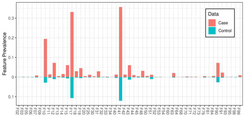
Figure 9 shows the prevalence of three-digit F chapter codes in cases and controls with the same case-control dataset used in constructing Table 5 in the main paper.

Figure 9: Suicide risk study: prevalence of three-digit ICD codes for a case-control data set.

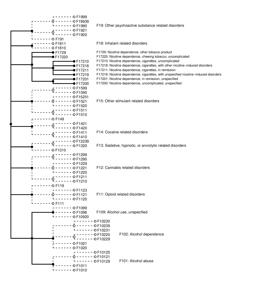
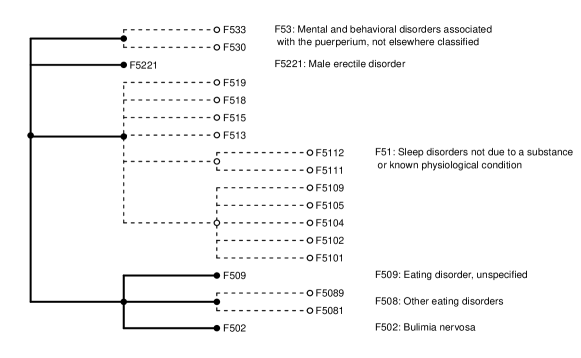
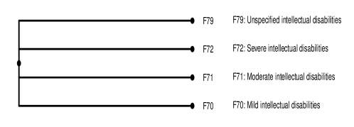
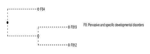
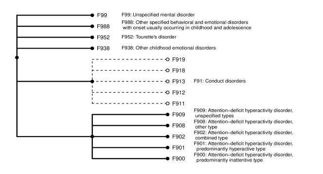
The aggregated structure from the TSLA framework can be shown in a tree format. A cross sign at the leaf node indicates that the corresponding feature can be dropped from the model. Features with closed leaf nodes are selected and left uncollapsed. The open leaf nodes are connected with dashed branches, where the corresponding features under the same closed node are aggregated. The ICD selection and aggregation patterns of F1, F2, F5, F6, F7, F8, and F9 are shown in Figures 10–16.

Figure 10: Suicide risk study: feature selection and aggregation in F1 codes.

Figure 11: Suicide risk study: feature selection and aggregation in F2 codes.

Figure 12: Suicide risk study: feature selection and aggregation in F5 codes.

Figure 13: Suicide risk study: feature selection and aggregation in F6 codes.

Figure 14: Suicide risk study: feature selection and aggregation in F7 codes.

Figure 15: Suicide risk study: feature selection and aggregation in F8 codes.

Figure 16: Suicide risk study: feature selection and aggregation in F9 codes.

Appendix E TripAdvisor User Rating Prediction with Review Texts

We consider the problem of predicting user review ratings (1 to 5) by the appearance of adjectives in each review. The data is from the R package rare (Yan and Bien, 2021), which contains a 500-by-200 document-term matrix for 200 adjectives appearing in 500 TripAdvisor reviews.

We begin by obtaining the tree structure between the adjectives. An “hclust” tree of the 200 adjectives, generated with 100-dimensional word embeddings pre-trained by GloVe is provided in the package. We cut the “hclust” tree into 2, 8, 32, 64, and 200 groups, and the resulting tree is of height 5. The document-term matrix is converted to a binary matrix of absence/presence, and 38 zero columns are removed.

We build two models under the logic aggregation framework. One is the TSLA model with all of the 162 nonzero features (TSLA). The other one is an elastic-net penalized linear regression model (TSLA-Enet) based on the resulting aggregated features from TSLA. We consider four competing models for comparison: RFS-Sum, Enet, Enet2, and LR. For each model, we compare the prediction performance with the out-of-sample mean squared error (MSE), which is measured with a random-splitting procedure over 10 repetitions. We use 300 observations for training and 200 observations for testing each time.

Figure 17: TripAdvisor user rating prediction: prediction performance based on a random-splitting procedure.

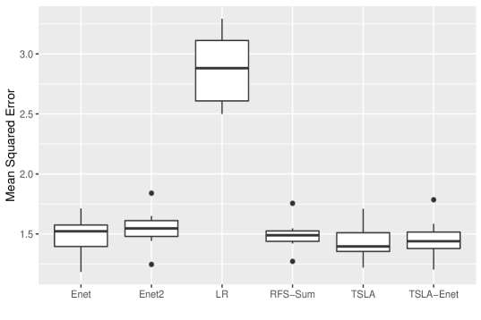
The out-of-sample MSE for each model is shown in Figure 17. TSLA and TSLA-Enet give the best prediction performance, followed by RFS-Sum. The results indicate that there exists a coarser tree structure. Furthermore, using structured information from the real data can be beneficial in prediction.

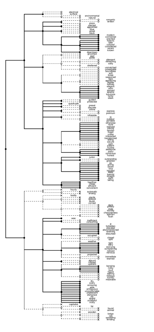
Figure 18 shows the selection and aggregation pattern of the 162 adjectives. The merging branches reveal that words of similar meaning and sentiment can be aggregated together. For example, the words describing colors: “blue”, “velvet”, and “black”, are aggregated into one predictor. The words “romantic”, “written”, and “piano” are also merged as they are related to hotel atmosphere. Some neutral words that do not convey strong sentiment, like “hourly”, “sprawling”, and “winding”, do not have much contribution to inform user ratings. Moreover, we notice that positive words of similar sentiment tend to be aggregated together, while most negative words tend to stay separated.

Figure 18: TripAdvisor user rating prediction: feature selection and aggregation.

References

- Albert and Anderson (1984) Albert, A. and J. A. Anderson (1984). On the existence of maximum likelihood estimates in logistic regression models. Biometrika 71(1), 1–10.
- Barak-Corren et al. (2017) Barak-Corren, Y., V. M. Castro, S. Javitt, A. G. Hoffnagle, Y. Dai, R. H. Perlis, M. K. Nock, J. W. Smoller, and B. Y. Reis (2017). Predicting suicidal behavior from longitudinal electronic health records. American Journal of Psychiatry 174(2), 154–162.
- Beck and Teboulle (2009) Beck, A. and M. Teboulle (2009). A fast iterative shrinkage-thresholding algorithm for linear inverse problems. SIAM Journal on Imaging Sciences 2(1), 183–202.
- Bühlmann and Van De Geer (2011) Bühlmann, P. and S. Van De Geer (2011). Statistics for High-Dimensional Data: Methods, Theory and Applications. Springer.
- Cartwright (2013) Cartwright, D. J. (2013). ICD-9-CM to ICD-10-CM codes: What? Why? How? Advances in Wound Care 2(10), 588–592.
- Chen and Aseltine (2017) Chen, K. and R. H. Aseltine (2017, aug). Using hospitalization and mortality data to identify areas at risk for adolescent suicide. Journal of Adolescent Health 61(2), 192–197.
- Chen et al. (2012) Chen, X., Q. Lin, S. Kim, J. G. Carbonell, and E. P. Xing (2012). Smoothing proximal gradient method for general structured sparse regression. The Annals of Applied Statistics 6(2), 719–752.
- Deschepper et al. (2019) Deschepper, M., K. Eeckloo, D. Vogelaers, and W. Waegeman (2019). A hospital wide predictive model for unplanned readmission using hierarchical ICD data. Computer Methods and Programs in Biomedicine 173(C), 177–183.
- Dome et al. (2019) Dome, P., Z. Rihmer, and X. Gonda (2019). Suicide risk in bipolar disorder: A brief review. Medicina (Kaunas, Lithuania) 55(8), 403.
- Forman et al. (2003) Forman, G. et al. (2003). An extensive empirical study of feature selection metrics for text classification. Journal of Machine Learning Research 3, 1289–1305.
- Fralick et al. (2019) Fralick, M., E. Sy, A. Hassan, M. J. Burke, E. Mostofsky, and T. Karsies (2019, 02). Association of concussion with the risk of suicide: A systematic review and meta-analysis. JAMA Neurology 76(2), 144–151.
- Haque et al. (2018) Haque, T. U., N. N. Saber, and F. M. Shah (2018). Sentiment analysis on large scale Amazon product reviews. In 2018 IEEE International Conference on Innovative Research and Development, pp. 1–6. IEEE.
- Hsu et al. (2012) Hsu, D., S. Kakade, and T. Zhang (2012). A tail inequality for quadratic forms of subgaussian random vectors. Electronic Communications in Probability 17, 1–6.
- Huang et al. (2008) Huang, A. et al. (2008). Similarity measures for text document clustering. In Proceedings of the Sixth New Zealand Computer Science Research Student Conference, pp. 9–56.
- Jovanovic et al. (2016) Jovanovic, M., S. Radovanovic, M. Vukicevic, S. Van Poucke, and B. Delibasic (2016). Building interpretable predictive models for pediatric hospital readmission using Tree-Lasso logistic regression. Artificial Intelligence in Medicine 72, 12–21.
- Koehler and Gan (1990) Koehler, K. J. and F. Gan (1990). Chi-squared goodness-of-fit tests: Cell selection and power. Communications in Statistics-Simulation and Computation 19(4), 1265–1278.
- Kooperberg et al. (2001) Kooperberg, C., I. Ruczinski, M. L. LeBlanc, and L. Hsu (2001). Sequence analysis using logic regression. Genetic Epidemiology 21(S1), S626–S631.
- Kozma et al. (2009) Kozma, L., A. Ilin, and T. Raiko (2009). Binary principal component analysis in the Netflix collaborative filtering task. In 2009 IEEE International Workshop on Machine Learning for Signal Processing, pp. 1–6. IEEE.
- Levy and Goldberg (2014) Levy, O. and Y. Goldberg (2014). Neural word embedding as implicit matrix factorization. In Proceedings of the 27th International Conference on Neural Information Processing Systems, pp. 2177–2185. MIT Press.
- Li et al. (2022) Li, G., Y. Li, and K. Chen (2022). It’s all relative: Regression analysis with compositional predictors. Biometrics. In press.
- Liu and Ye (2010) Liu, J. and J. Ye (2010). Moreau-Yosida regularization for grouped tree structure learning. In Proceedings of the 23rd International Conference on Neural Information Processing Systems, pp. 1459–1467. MIT Press.
- Liu et al. (2021) Liu, L., H. Gu, J. Van Limbergen, and T. Kenney (2021). SuRF: A new method for sparse variable selection, with application in microbiome data analysis. Statistics in Medicine 40(4), 897–919.
- Lucek and Ott (1997) Lucek, P. R. and J. Ott (1997). Neural network analysis of complex traits. Genetic Epidemiology 14(6), 1101–1106.
- Miller and Black (2020) Miller, J. N. and D. W. Black (2020). Bipolar disorder and suicide: A review. Curr Psychiatry Rep 22(2), 6.
- Mukherjee et al. (2015) Mukherjee, R., N. S. Pillai, and X. Lin (2015). Hypothesis testing for high-dimensional sparse binary regression. The Annals of Statistics 43(1), 352–381.
- Naumov et al. (2021) Naumov, S., G. Yaroslavtsev, and D. Avdiukhin (2021). Objective-based hierarchical clustering of deep embedding vectors. In Proceedings of the AAAI Conference on Artificial Intelligence, pp. 9055–9063. The AAAI Press.
- Nepon et al. (2010) Nepon, J., S.-L. Belik, J. Bolton, and J. Sareen (2010). The relationship between anxiety disorders and suicide attempts: Findings from the national epidemiologic survey on alcohol and related conditions. Depression and anxiety 27(9), 791–798.
- Nesterov (1983) Nesterov, Y. (1983). A method for unconstrained convex minimization problem with the rate of convergence . Doklady AN SSSR (translated as Soviet Math. Docl.) 269, 543–547.
- Nesterov (2005) Nesterov, Y. (2005). Smooth minimization of non-smooth functions. Mathematical Programming 103(1), 127–152.
- Patrick et al. (2010) Patrick, A. R., M. Miller, C. W. Barber, P. S. Wang, C. F. Canning, and S. Schneeweiss (2010, dec). Identification of hospitalizations for intentional self-harm when E-codes are incompletely recorded. Pharmacoepidemiology and Drug Safety 19(12), 1263–1275.
- Ruczinski et al. (2003) Ruczinski, I., C. Kooperberg, and M. LeBlanc (2003). Logic regression. Journal of Computational and Graphical Statistics 12(3), 475–511.
- Ruczinski et al. (2004) Ruczinski, I., C. Kooperberg, and M. L. LeBlanc (2004). Exploring interactions in high-dimensional genomic data: An overview of logic regression, with applications. Journal of Multivariate Analysis 90(1), 178–195.
- Saeys et al. (2007) Saeys, Y., I. Inza, and P. Larranaga (2007). A review of feature selection techniques in bioinformatics. Bioinformatics 23(19), 2507–2517.
- Schloss et al. (2009) Schloss, P. D., S. L. Westcott, T. Ryabin, J. R. Hall, M. Hartmann, E. B. Hollister, R. A. Lesniewski, B. B. Oakley, D. H. Parks, C. J. Robinson, et al. (2009). Introducing mothur: Open-source, platform-independent, community-supported software for describing and comparing microbial communities. Applied and Environmental Microbiology 75(23), 7537–7541.
- Schwender and Ickstadt (2008) Schwender, H. and K. Ickstadt (2008). Identification of SNP interactions using logic regression. Biostatistics 9(1), 187–198.
- She (2010) She, Y. (2010). Sparse regression with exact clustering. Electronic Journal of Statistics 4, 1055–1096.
- Simon et al. (2018) Simon, G. E., E. Johnson, J. M. Lawrence, R. C. Rossom, B. Ahmedani, F. L. Lynch, A. Beck, B. Waitzfelder, R. Ziebell, R. B. Penfold, and S. M. Shortreed (2018). Predicting suicide attempts and suicide deaths following outpatient visits using electronic health records. American Journal of Psychiatry 175(10), 951–960.
- Su et al. (2020) Su, C., R. Aseltine, R. Doshi, K. Chen, S. C. Rogers, and F. Wang (2020). Machine learning for suicide risk prediction in children and adolescents with electronic health records. Translational Psychiatry 10(1), 413.
- Tibshirani (2015) Tibshirani, R. J. (2015). A general framework for fast stagewise algorithms. Journal of Machine Learning Research 16(1), 2543–2588.
- van de Geer (2008) van de Geer, S. A. (2008). High-dimensional generalized linear models and the lasso. The Annals of Statistics 36(2), 614–645.
- Walsh et al. (2017) Walsh, C. G., J. D. Ribeiro, and J. C. Franklin (2017). Predicting risk of suicide attempts over time through machine learning. Clinical Psychological Science 5(3), 457–469.
- Wei and Huang (2010) Wei, F. and J. Huang (2010). Consistent group selection in high-dimensional linear regression. Bernoulli 16(4), 1369–1384.
- Yan and Bien (2021) Yan, X. and J. Bien (2021). Rare feature selection in high dimensions. Journal of the American Statistical Association 116(534), 887–900.