AppdxReferences
Constrained Submodular Optimization for Vaccine Design
Abstract
Advances in machine learning have enabled the prediction of immune system responses to prophylactic and therapeutic vaccines. However, the engineering task of designing vaccines remains a challenge. In particular, the genetic variability of the human immune system makes it difficult to design peptide vaccines that provide widespread immunity in vaccinated populations. We introduce a framework for evaluating and designing peptide vaccines that uses probabilistic machine learning models, and demonstrate its ability to produce designs for a SARS-CoV-2 vaccine that outperform previous designs. We provide a theoretical analysis of the approximability, scalability, and complexity of our framework.
1 Introduction
Peptide vaccines that expand and activate T cells have emerged as a promising prophylactic and therapeutic approach for addressing health related challenges including infectious diseases and cancer (Malonis, Lai, and Vergnolle 2019). In contrast to more conventional live-attenuated vaccines that are based on entire organisms, or subunit vaccines that are based on entire protein subunits, peptide vaccines are based on a small set of protein fragments (peptides) that are sufficient to induce a T cell immune response, enabling the elicitation of far more targeted responses that avoid allergenic and reactogenic responses (Li et al. 2014).
The design of a peptide vaccine consists of selecting immunogenic protein fragments, usually referred to as epitopes (Li et al. 2014), that when included in a vaccine expand epitope specific T cells. Advances in machine learning have enabled our ability to predict which peptides will be presented by major histocompatibilty complex (MHC) molecules for surveillance by the adaptive immune system (Ching et al. 2018; Reynisson et al. 2020), which can be used to identify which epitopes will be displayed (Sohail et al. 2021).
The epitopes displayed by an individual depend upon the specific alleles of their MHC genes, and thus the peptides displayed by the immune system can vary greatly from individual to individual (Zaitouna, Kaur, and Raghavan 2020). Therefore, the engineering task of finding a set of peptides that is predicted to be displayed by a large portion of the population remains challenging despite progress on the peptide-MHC display task.
In this work we introduce a framework for evaluating and designing peptide vaccines that uses probabilistic interpretations of machine learning models, and demonstrate its ability to produce designs for the SARS-CoV-2 vaccine design task that outperform previous designs. We complement this with a theoretical analysis of the approximability, scalability, and complexity of our framework, which may be of independent interest.
1.1 Our contribution
To improve the effectiveness of a vaccine it is important to introduce redundancies into its design so the failure of a single displayed peptide to elicit an immune response does not become a single point of failure (Liu et al. 2021). Vaccines designed with an -times coverage objective aim to obtain at least immunogenic peptide “hits” in each person. Having more than one “hit” provides redundancy to expand multiple T cell clonotypes in an individual to fight disease, protects against peptide sequence drift resulting from pathogen or tumor mutations, protects against the loss of an MHC gene, and accounts for the variability of peptide immunogenicity between individuals.
We show that optimizing the population coverage for strict -times coverage guarantees cannot be tractably approximated to any constant factor assuming the intractability of the Gap-Small-Set Expansion problem (Raghavendra and Steurer 2010), a result which may be of independent interest. We therefore propose a diminishing returns framework that uses a soft redundancy guarantee as its objective. The resulting objective is both submodular and monotonic, and can therefore be approximated via a greedy approach which we call Optivax-P. We supplement the theoretical improvement with an empirical comparison of vaccines designed using our approach and previous designs. Our proposed framework also contributes the following desirable properties: it makes explicit the utility of having redundancy, does not discount the benefits of being covered without redundancy, and is able to reason with uncertainty. We demonstrate how uncertainty values for epitope identification can be derived by calibrating state-of-the-art peptide-MHC display predictors.
While redundancies in a design are important, it is also important that they be dissimilar redundancies, since reasons for failure may be shared between similar peptides. This additional constraint that selected peptides be dissimilar is problematic as it allows the problem formulation to encode NP-hard graph problems that in general cannot be approximated to any constant factor. However, by parameterizing on the structure of the constraints, we can derive lower bounds for the performance of the greedy approach which show that the greedy approach can still provide approximation guarantees under certain assumptions. These bounds may also be of independent interest.
1.2 Related work
The use of computational methods to aid vaccine design has taken on an increasingly important role in the vaccine design process over the past two decades (Moise et al. 2015). Much of the advancement stems from improvements in the epitope identification task, which has seen impressive improvements with advances in data collection strategies and machine learning (Ching et al. 2018; Reynisson et al. 2020). While good epitope prediction tools are essential to vaccine design, the focus of this work is on the downstream task of calibrating the predictions and selecting defined epitopes for vaccine inclusion.
Earlier works on vaccine design are reviewed in Oyarzun and Kobe (2015), and employ discrete optimization techniques such as integer linear programming and genetic algorithms to optimize population coverage. However, they do not anticipate or solve the problem of coverage with dissimilar redundancies (Liu et al. 2021), which we do in this work. Furthermore, they do not consider the epistemic uncertainty associated with epitope predictions, which we do.
Our work is closely related to the work in (Liu et al. 2021), where the use of an objective that accounts for dissimilar redundancies is proposed. However, approximating their proposed objective to any constant factor appears to be an intractable problem, while our objective permits constant factor approximations in polynomial time. Our framework also allows for reasoning about redundancies with uncertainty, which theirs does not.
1.3 Presentation
In the remaining four sections of the paper we present the optimization problem that we wish to solve (Section 2), provide an algorithm for solving the problem and analyze its runtime and approximation guarantees (Section 3), apply our framework to the SARS-CoV-2 vaccine design problem (Section 4), and conclude with a discussion (Section 5). Theorems are presented where appropriate throughout. Proofs, including intuitive descriptions, are relegated to Appendix A for improved flow.
2 A diminishing returns objective enables theoretical performance guarantees
Our goal in this section is to formalize the vaccine design problem as an optimization problem. We first show theoretical barriers to obtaining performance guarantees for previous formalizations, and then introduce the diminishing returns framework which addresses this.
Peptide vaccines are designed by considering the peptide sequence(s) of a target of interest, for example the proteome of a virus, and selecting a small set of peptides within the target sequences to include in the vaccine. Vaccine peptides are selected such that they elicit an immune response in a large portion of a susceptible population that we wish to vaccinate. This is done by selecting vaccine peptides that are displayed on the cell surface by MHC proteins. The resulting peptide-MHC complexes activate the cellular immune system. The challenge of selecting a set of peptides arises from the polymorphism present in MHCs within a population. Different MHC alleles have different peptide binding properties, so the peptides must be carefully chosen in order to elicit widespread immune responses from a given population.
2.1 Preliminaries
Let denote non-negative real numbers. Let be some finite set of elements. Let . We say is submodular if whenever and , and we say that is monotonically increasing if for all .
Suppose is a graph. For simplicity, we will at times use to denote its vertex set and to denote its edge set . The th power of , denoted , is defined as the graph , where and contains all pairs of vertices between which there exists a path of length less than or equal to in .
We will use to denote an indicator that evaluates to 1 if is true and 0 otherwise for any proposition .
2.2 Optimizing population coverage with redundancies is computationally difficult
It is important for a vaccine to cause the display of multiple epitopes in individuals to provide redundancy in the activation of T cell clonotypes, to expand multiple T cell clonotypes in an individual to fight disease, to protect against peptide sequence drift as a consequence of pathogen or tumor mutations, to protect against the loss of an MHC gene, and to account for the variability of peptide immunogenicity between individuals (Liu et al. 2021). In Liu et al. (2021), the authors showed that previous vaccine designs fail to cover significant portions of the population when coverage criteria include these redundancies. To address this, they introduce the -times coverage framework, which involves solving the max -times coverage problem. The problem is defined as follows:
Definition 1.
Given a ground set, a set of weights over the ground set, a collection of multisets whose elements are from the ground set, and some cardinality constraint , find a collection of multisets such that the aggregate weights of the elements in the ground set that are covered at least times is maximized.
The sum of the weights of the the elements that are covered at least times is then called the -times coverage. For vaccine design, the ground set corresponds to MHC genotypes, the weights correspond to the percentage of the population with the genotypes, and each multiset corresponds to a peptide, which covers certain genotypes a variable number of times. Solving this problem with cardinality constraint then gives a vaccine design consisting of peptides, with the objective that a large portion of the population display at least peptides (i.e. have at least peptide-MHC hits).
While this is a natural extension of earlier vaccine design paradigms that do not account for redundancies, it is a computationally difficult problem. The authors have shown in their work that this is an NP-hard optimization problem, and so they propose heuristic approaches. However their proposed approaches have no performance guarantees. Here, we show that this problem is related to Gap-Small-Set Expansion, which suggests that finding any constant factor approximation cannot be achieved in polynomial time.
Theorem 1.
For any , if there exists a polynomial time algorithm that can achieve an approximation factor of to max -times coverage, then there exists a polynomial time algorithm that can decide for some .
There is currently no known polynomial time algorithm for for any . The Small Set Expansion Hypothesis conjectures that is NP-hard for any , and is currently an open problem related to the Unique Games Conjecture (Raghavendra and Steurer 2010).
2.3 A diminishing returns framework for vaccine design provides a submodular optimization objective
A key reason underlying the complexity of the max -times coverage problem is that the utility of a peptide may be hidden until we are close to reaching -times coverage. This makes it difficult select peptides optimally before its utility becomes apparent. To address this, we propose a diminishing returns framework, where peptides will improve the objective at any coverage level. Intuitively, this provides a “gradient” along which an optimization procedure can climb.
Formally, let be some non-negative monotonically increasing concave function such that . Let denote the set of MHC genotypes observed in the population. Let be a weight function that gives the frequency of each genotype in the population. Let denote the set of candidate peptides from which a subset is selected for the vaccine design. If and , let denote the predicate of whether is displayed in an individual with genotype . To model uncertainty, we let vary over the sample space of some probability space, and we assume that the subset of the probability space where evaluates to true is always measurable. The objective, parametrized by , can then be written as follows:
| (1) |
Where is the set of peptides selected for vaccine inclusion. This objective is a monotonically increasing submodular function.
Theorem 2.
For any that is monotonically increasing and concave, is a monotonically increasing submodular function.
As a consequence, we can attain a -factor approximation using the greedy approach if no additional constraints are given aside from the cardinality of the peptide set (Nemhauser, Wolsey, and Fisher 1978). Beyond submodularity, this objective contributes the following desirable properties: first, it accounts for the fact that having peptide-MHC hits is useful, even if the redundancy does not obtain a given threshold. While having high redundancy is better than having low redundancy, having low redundancy is better than not displaying any peptides. Second, the utility we expect from attaining a given number of peptide-MHC hits is made explicit through . Third, it allows reasoning with uncertainty by allowing to be an uncertain event. Many prediction models output a soft classification instead of a hard one, which we can calibrate to attach uncertainties to the classifications.
For an arbitrary distribution over the set of indicator variables we may need to approximate the expectation in via sampling. However, we can compute the objective exactly and efficiently if we suppose that for a given MHC genotype , the set of indicator variables are independent. This is almost certainly false given a sufficiently large pool of peptide sequences, since we should be able to significantly improve the performance of a predictor by training it on a sufficiently large number of peptide sequences. However, we can weaken this assumption to -wise independence if we only consider vaccine designs that include at most peptides. For values of that are reasonable in the context of designing peptide vaccines, this assumption is more reasonable than the full independence assumption.
Under the independence assumption we can calculate the objective by computing the distribution of the sum via iterated convolutions of Bernoulli distributions, and then taking the expectation using the distribution (see Appendix C for additional details). This runs in time , where is the number of genotypes and is the number of peptides in the vaccine design.
2.4 Peptide selections need to be constrained to avoid unreasonable designs
We impose two types of constraints on the set of peptides selected for vaccine inclusion: a cardinality constraint, and a set of pairwise constraints.
The cardinality constraint is necessary since our objective function is monotonically increasing. Therefore, the full set of candidate peptides will maximize it. This is undesirable, since peptide vaccines need to be compact to permit effective delivery and to induce effective intolerance in the context of limited immune system capacity. Therefore, we will impose a cardinality constraint on the set of selected peptides such that it cannot exceed a given size .
The pairwise constraints are required to avoid very similar peptides from being included. Peptide candidates for vaccine inclusion are generated by sliding windows of various sizes across the protein sequence we wish to target. The produces peptides that are highly similar in sequence, such as nested sequences, and including highly related sequences does not truly improve the effectiveness of the vaccine. Furthermore, the assumption that the variables indicating peptide-MHC interactions are independent likely does not hold when peptides are very similar, since it is possible that the predictor makes use of similar features, which result in systematic errors. Therefore, we introduce a set of pairwise constraints as a graph where the vertex set , and where edges exist between peptides that are deemed redundant. We then require that the peptides in the vaccine design form an independent set within .
3 Methods
3.1 A greedy approach provides performance guarantees under the diminishing returns framework
Our goal is the following: given a peptide set , a set of MHC genotypes , binding credences between all peptides and MHCs, a monotonically increasing concave utility function with , a cardinality constraint , and pairwise constraints , find a set that satisfies all the constraints and maximizes the objective function . We define the binding credence between a peptide and an MHC as the measure of the subset of the probability space where evaluates to true. Practically, these values behave like probabilities. We use the term credence to emphasize the epistemic nature of the uncertainty.
We present Optivax-P, a greedy approach outlined in Algorithm 1, to produce a solution to this problem. The procedure is straightforward: at each iteration we add the peptide that maximally improves the solution to the solution set, then eliminate that peptide and all similar peptides from consideration for all future steps.
Runtime analysis of Optivax-P
The naive runtime is : the objective function is evaluated times to compute the , the is computed at most times, and each evaluation of the objective function takes time since the designs will never contain more than elements.
We can improve the runtime by evaluating the marginal improvement rather than the full objective, bringing the overall runtime down to (see Appendix C). We can further vectorize the computation to evaluate the in vector operations, reducing the runtime to vector operations and operations for constraint handling (see Appendix C). However, vector operations require batching if and are large, so those parameters still play a significant role in the runtime.
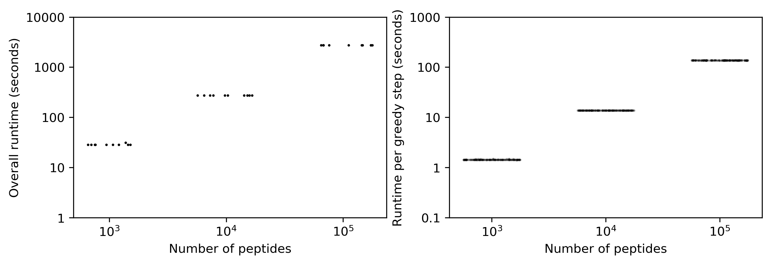
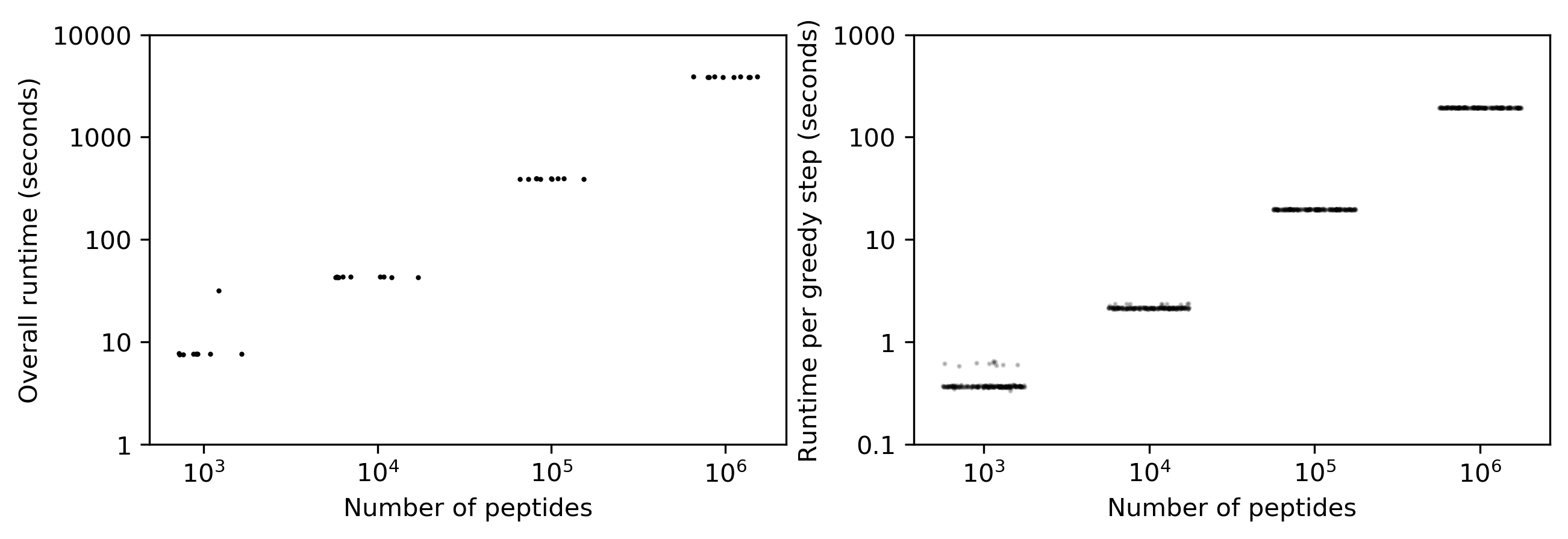
Our implementation can generate designs of size over a peptide set of size with genotypes in approximately 5 minutes when parallelized over 8 Titan RTX GPUs. See Appendix C for additional details.
Approximation ratio of Optivax-P
Let denote the true optimum of the optimization problem. If we let each peptide and MHC genotype interact with probability 1 and let be sufficiently large, then the desired optimization is equivalent to finding the maximum independent set within . Finding any constant factor approximation to max-clique is NP-hard (Zuckerman 2006), which then immediately implies that cannot be approximated to any constant factor. Therefore, the quality of the solution produced by Optivax-P cannot be unconditionally bounded by a constant factor with respect to , since Optivax-P runs in polynomial time.
However, we can bound the solution by looking at the graph structure of . Since we are considering cases where similarity relations are mostly generated from sliding windows over linear sequences, we might expect the resulting graph to be of low degree. Let denote the degree of . Note that in the special case where , there are no pairwise constraints, so the problem reduces to the optimization of a monotonic submodular function under a cardinality constraint. It is well established that the greedy approach attains an approximation ratio of in this case (Nemhauser, Wolsey, and Fisher 1978), and that attaining an approximation ratio of for any is NP-hard (Feige 1998).
Another property we can look at is the graph power of . We may expect that in the case where a graph looks like a path, taking the graph power would not add too many extra constraints, in which case replacing with its graph power would not yield a optimum that is too different. Let denote the solutions to the more constrained optimizations:
| (2) |
We can then bound the output of Optivax-P by incorporating these extra graph parameters:
Theorem 3.
Let be the output of Optivax-P. Then:
-
1.
If , then
-
2.
If , then
We can upper bound the best possible performance of polynomial time algorithms.
Theorem 4.
Unless P = NP, there exists no polynomial time algorithm that can output an approximation that guarantees either of the following on all inputs for any :
-
1.
-
2.
3.2 Using machine learning based models to attain binding credences
We define as a random event in a probability space of beliefs that peptide is presented by MHC genotype . We use well established state-of-the-art neural network based models (NetMHCpan4.1 and NetMHCpanII4.0 (Reynisson et al. 2020)) to generate predictions that we use to derive . We will assume that the derived beliefs are independent (although it is sufficient to assume -wise independence, and only between events that share a genotype - see Section 2.3). While this may not necessarily be true for closely related sequences, we circumvent this by constraining our designs so that they do not contain closely related sequences (see Section 2.4).
There are two classes of MHC molecules that we need to design our vaccine to bind to. However, due to molecular differences between the two molecules the peptides they bind are largely disjoint. We can therefore simplify the problem to that of producing two separate designs, one for Class I MHCs and one for Class II MHCs. NetMHCpan4.1 provides predictions between peptides and Class I MHCs while NetMHCIIpan4.0 provides predictions between peptides and Class II MHCs. For simplicity, we will refer to these predictors together as NetMHCpan.
Having fixed our class of interest, we then define an MHC genotype to be a set of 3-6 distinct alleles. NetMHCpan provides binding predictions between peptides and individual alleles rather than genotypes, so to attain credences for whether a peptide is displayed by a genotype we assume independence between our beliefs that the peptides are displayed by individual alleles and compute the credence as the following:
| (3) |
Where is the credence for binding between a peptide and a specific allele .
NetMHCpan outputs likelihoods for binding between any given peptide and any given MHC molecule . However, it is important to ensure that this likelihood is well calibrated. By default, NetMHCpan calibrates itself by comparing the scores it outputs against a repertoire of naturally occurring peptides and classifying a sequence as being displayed if it scores higher than 99.5% of those peptides when characterizing binding to Class I MHC and 98% of those peptides when classifying binding to Class II MHC.
To attain well calibrated credences, we make use of publicly available datasets that were used to validate NetMHCpan, which contain no overlap with the dataset used to train NetMHCpan (Reynisson et al. 2020). The dataset consists of a set of epitopes, the MHC molecule they bind to, and the natural context they occur in. The epitopes were used as positive samples while the context sequences were used to generate negative samples. The samples were weighted such that the ratio of the weight of all positive samples to that of all negative samples is for Class I MHC and for Class II MHC to match the fraction of natural peptides that NetMHCpan implicitly assumes to be binders. The samples were then all fed into NetMHCpan to produce predictions. See Appendix B for additional details. The samples were then binned into 20 equally sized bins and the weighted fraction of positive samples within each bin was calculated to produce a calibration curve, which we present in Figure 1A. We then generate a calibration function by minimizing the following objective:
A)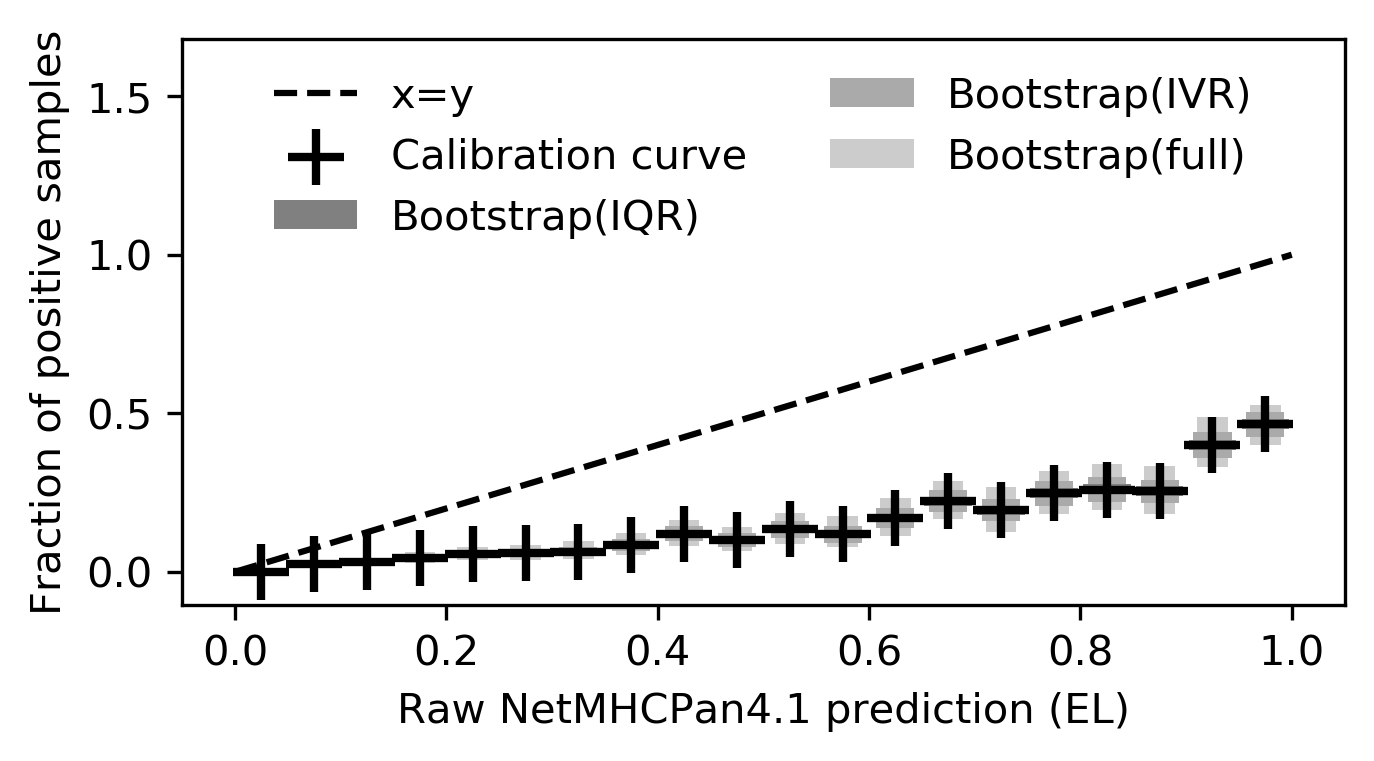 B)
B)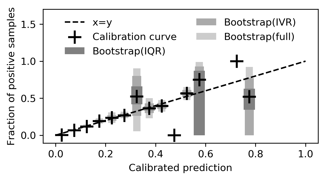
| (4) |
Where all samples are indexed by an integer between 1 and , denotes the NetMHCpan predicted value of the sample, is 1 if the sample is positive and 0 if the sample is negative, and is the weight assigned to the sample. The samples are ordered such that for all , so can be interpreted as the window size. We constrain to be non-decreasing and non-negative, so this is a form of isotonic regression. Additional details can be found in Appendix B.
If NetMHCpan outputs on an input peptide and MHC , we set our credence that binds to as . A calibration curve of the calibrated predictions of the validation dataset is shown in Figure 1B.
4 Results
4.1 Greedy selection outperforms baseline methods
Optivax-P has good worst case theoretical guarantees which are even optimal in the absence of pairwise constraints unless P=NP. Here we empirically check its performance against two baseline approaches in random settings. The first baseline is the random approach, where peptides are chosen randomly. The second baseline is via linear approximation, where the concave function in Equation 1 is removed to produce a surrogate objective. This surrogate is linear, so it can be trivially optimized to produce a solution.
We compare the algorithms by generating peptide vaccine designs of 64 different sizes in 2000 randomly generated settings, where each setting randomizes the number of genotypes and peptides, the display credences, and the concave function in the objective (Equation 1). Details can be found in Appendix D. We find that Optivax-P outperforms the baselines in most settings (Figure 2).

4.2 Designing a SARS-CoV2 vaccine with Optivax-P
We apply Optivax-P in a practical setting by producing vaccine designs for SARS-CoV2. To design our vaccine, we use a set of candidate peptides sourced from Liu et al. (2021) which includes peptides from SARS-CoV2 that have been filtered for undesirable properties like high mutation rates, cleavage, and glycosylation. Peptides that were present in the human proteome were also removed, since they may trigger adverse autoimmune responses. Liu et al. (2021) have also published a set of genotypes and their frequencies which we use. These frequencies are derived from diverse populations and have been selected to be representative of the global population. We calculated binding credences for each peptide-genotype pair as described in Section 3.2. Additionally, if a peptide was not present in representative genomes of the Omicron BA.1 and Omicron BA.2 variants of SARS-CoV2 (accession number OM873778 and OW123901 respectively, both retrieved from the The COVID-19 Data Portal (Harrison et al. 2021)) then we set the credence of that peptide being displayed on any MHC molecule to 0.
We applied Optivax-P to design vaccines with peptide sets of size 1 and 150 inclusive. Designs were constrained such that no pair of peptides can be within 3 edits (insertions, deletions, or substitutions) of each other for the MHC Class I design, and 5 edits for the MHC Class II design. Designs were optimized for the objective for between 1 and 20 inclusive, where is defined as:
| (5) |
can be viewed as a threshold parameter. This corresponds to a model where each peptide-MHC hit provides incremental protection until a person attains hits, at which point they are fully protected and stop seeing additional benefits. A comparison between Optivax-P designs and previous designs is shown in Figure 3, where we can see all Optivax-P designs score substantially higher on . Evaluations on for other show similar trends and are presented in Appendix D.
A)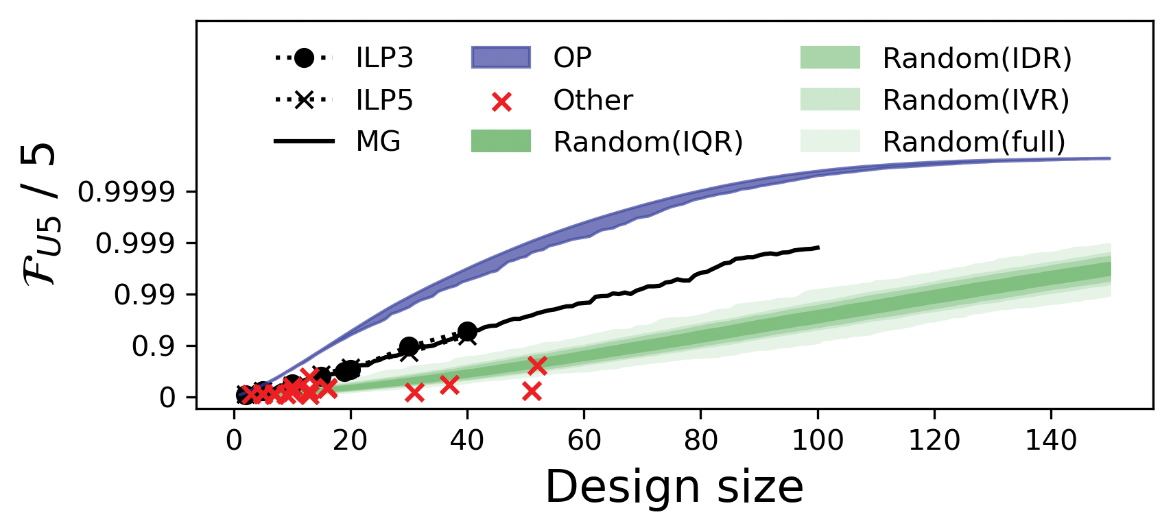 B)
B)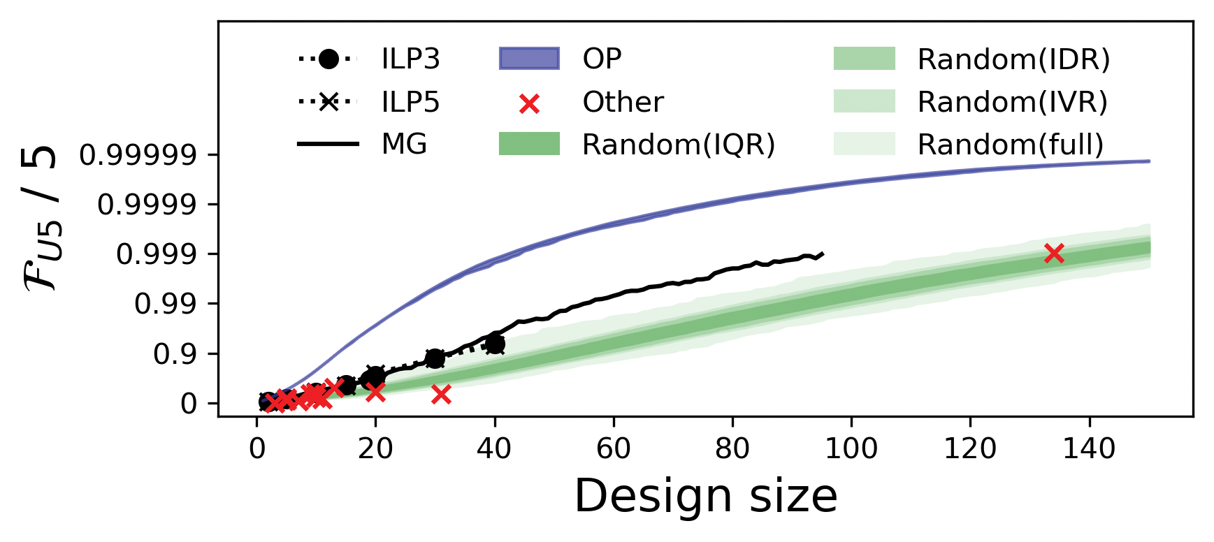
While this demonstrates that our optimization procedure works and that there are deficiencies in previous designs that are addressed through our designs if our utility model is reflective of reality, it may not be entirely surprising that vaccine designs optimized for score well on , even for mismatching . To control for this, we also evaluate designs produced by Optivax-P on the -times coverage objective proposed by Liu et al. (2021) and described in Section 2.2. We modify our credences such that they are only 0 or 1, and such that they closely match the values used by Liu et al. (2021) (i.e. if and only if the genotype is present within the peptide , where peptides are viewed as multisets of genotypes in the max -times coverage framework).
We then produced designs of size 19 using for all between 1 and 10 inclusive. These designs were then assigned a score equal to their -times coverage for between 1 and 20 inclusive. In Figure 4 we compare these scores to the scores attained by designs generated by Liu et al. (2021), which also each contain 19 peptides. We see that Optivax-P is highly competitive even when evaluated on a objective separate from the one it was optimized for.
A)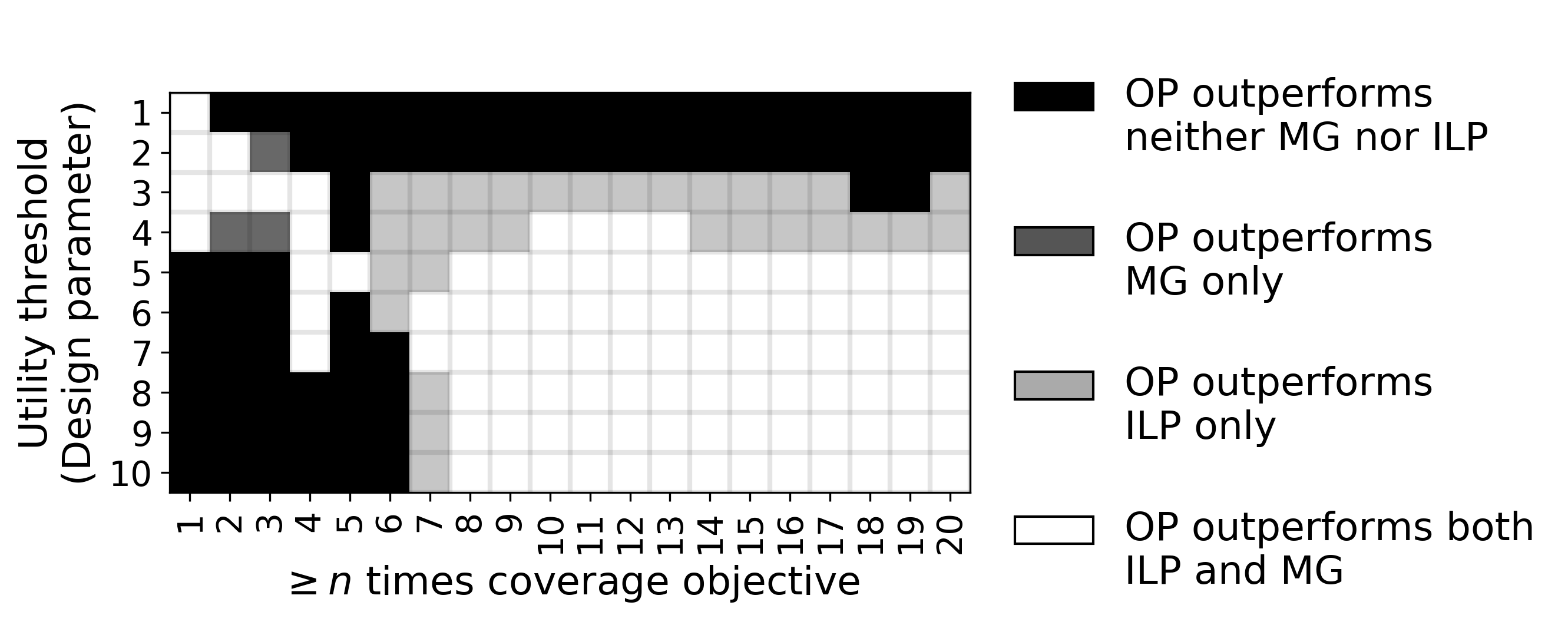 B)
B)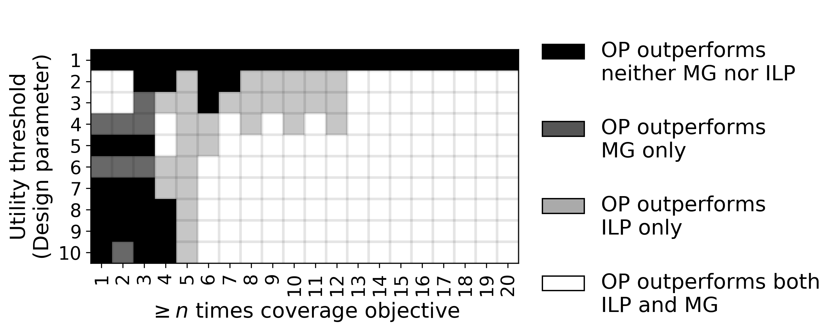
5 Discussion
We have introduced the diminishing returns framework and Optivax-P for designing epitope based peptide vaccines. The framework is based on constrained submodular optimization, which permits Optivax-P to provide performance guarantees despite the NP-hardness of the problem, unlike previous approaches. We also show how we can probabilistically interpret the outputs of machine learning models to allow reasoning with uncertainty within the framework. Finally, we demonstrated that Optivax-P achieves superior performance against past vaccine designs on the SARS-CoV-2 vaccine design task, and achieves comparable performance even when evaluated against previous objectives.
Optivax-P is highly scalable, allowing us to optimize over potentially millions of candidate peptides for a single vaccine. The ability to reason with uncertainty also gives us a much richer language for expressing the properties of a peptide: for instance, instead of filtering out peptides prone to mutation, we can consider the probability of sequence drift. These factors allow us to consider a far wider range of peptide vaccine design tasks, which we plan to use in the future.
Acknowledgements
This work was supported in part by Schmidt Futures and a C3.ai grant. The authors would also like to thank Ge Liu, Alexander Dimitrakakis, Brandon Carter, and members of the Gifford lab for useful discussions and feedback.
References
- Abdelmageed et al. (2020) Abdelmageed, M.; Abdelmoneim, A.; Mustafa, M.; Elfadol, N.; Murshed, N.; Shantier, S.; and Makhawi, A. 2020. Design of multi epitope-based peptide vaccine against E protein of human 2019-nCoV: An immunoinformatics approach. bioRxiv 2020. Preprint, 1–21.
- Ahmed, Quadeer, and McKay (2020) Ahmed, S. F.; Quadeer, A. A.; and McKay, M. R. 2020. Preliminary identification of potential vaccine targets for the COVID-19 coronavirus (SARS-CoV-2) based on SARS-CoV immunological studies. Viruses, 12(3): 254.
- Akhand et al. (2020) Akhand, M. R. N.; Azim, K. F.; Hoque, S. F.; Moli, M. A.; Joy, B. D.; Akter, H.; Afif, I. K.; Ahmed, N.; and Hasan, M. 2020. Genome based evolutionary study of SARS-CoV-2 towards the prediction of epitope based chimeric vaccine. BioRxiv.
- Alam et al. (2020) Alam, A.; Khan, A.; Imam, N.; Siddiqui, M. F.; Waseem, M.; Malik, M. Z.; and Ishrat, R. 2020. Design of an epitope-based peptide vaccine against the severe acute respiratory syndrome coronavirus-2 (SARS-CoV-2): a vaccine-informatics approach. BioRxiv.
- Banerjee, Santra, and Maiti (2020) Banerjee, A.; Santra, D.; and Maiti, S. 2020. Energetics based epitope screening in SARS CoV-2 (COVID 19) spike glycoprotein by Immuno-informatic analysis aiming to a suitable vaccine development. bioRxiv.
- Baruah and Bose (2020) Baruah, V.; and Bose, S. 2020. Immunoinformatics-aided identification of T cell and B cell epitopes in the surface glycoprotein of 2019-nCoV. Journal of medical virology, 92(5): 495–500.
- Bhattacharya et al. (2020) Bhattacharya, M.; Sharma, A. R.; Patra, P.; Ghosh, P.; Sharma, G.; Patra, B. C.; Lee, S.-S.; and Chakraborty, C. 2020. Development of epitope-based peptide vaccine against novel coronavirus 2019 (SARS-COV-2): Immunoinformatics approach. Journal of medical virology, 92(6): 618–631.
- Ching et al. (2018) Ching, T.; Himmelstein, D. S.; Beaulieu-Jones, B. K.; Kalinin, A. A.; Do, B. T.; Way, G. P.; Ferrero, E.; Agapow, P.-M.; Zietz, M.; Hoffman, M. M.; et al. 2018. Opportunities and obstacles for deep learning in biology and medicine. Journal of The Royal Society Interface, 15(141): 20170387.
- Fast, Altman, and Chen (2020) Fast, E.; Altman, R. B.; and Chen, B. 2020. Potential T-cell and B-cell epitopes of 2019-nCoV. BioRxiv.
- Feige (1998) Feige, U. 1998. A threshold of ln n for approximating set cover. Journal of the ACM (JACM), 45(4): 634–652.
- Gupta, Mishra, and Niraj (2020) Gupta, E.; Mishra, R. K.; and Niraj, R. R. K. 2020. Identification of potential vaccine candidates against SARS-CoV-2, A step forward to fight COVID-19: A Reverse Vaccinology Approach. bioRxiv.
- Harrison et al. (2021) Harrison, P. W.; Lopez, R.; Rahman, N.; Allen, S. G.; Aslam, R.; Buso, N.; Cummins, C.; Fathy, Y.; Felix, E.; Glont, M.; et al. 2021. The COVID-19 Data Portal: accelerating SARS-CoV-2 and COVID-19 research through rapid open access data sharing. Nucleic acids research, 49(W1): W619–W623.
- Herst et al. (2020) Herst, C. V.; Burkholz, S.; Sidney, J.; Sette, A.; Harris, P. E.; Massey, S.; Brasel, T.; Cunha-Neto, E.; Rosa, D. S.; Chao, W. C. H.; et al. 2020. An effective CTL peptide vaccine for Ebola Zaire Based on Survivors’ CD8+ targeting of a particular nucleocapsid protein epitope with potential implications for COVID-19 vaccine design. Vaccine, 38(28): 4464–4475.
- Lee and Koohy (2020) Lee, C. H.; and Koohy, H. 2020. In silico identification of vaccine targets for 2019-nCoV. F1000Research, 9.
- Li et al. (2014) Li, W.; Joshi, M. D.; Singhania, S.; Ramsey, K. H.; and Murthy, A. K. 2014. Peptide vaccine: progress and challenges. Vaccines, 2(3): 515–536.
- Liu et al. (2021) Liu, G.; Dimitrakakis, A.; Carter, B.; and Gifford, D. 2021. Maximum n-times Coverage for Vaccine Design. In International Conference on Learning Representations.
- Malonis, Lai, and Vergnolle (2019) Malonis, R. J.; Lai, J. R.; and Vergnolle, O. 2019. Peptide-based vaccines: current progress and future challenges. Chemical reviews, 120(6): 3210–3229.
- (18) Mitra, D.; Pandey, J.; and Swaroop, S. ???? Multi-epitope-based peptide vaccine design against SARS-CoV-2 using its spike protein, BioRxiv.(2020) 2020.04. 23.055467.
- Moise et al. (2015) Moise, L.; Gutierrez, A.; Kibria, F.; Martin, R.; Tassone, R.; Liu, R.; Terry, F.; Martin, B.; and De Groot, A. S. 2015. iVAX: An integrated toolkit for the selection and optimization of antigens and the design of epitope-driven vaccines. Human vaccines & immunotherapeutics, 11(9): 2312–2321.
- Nemhauser, Wolsey, and Fisher (1978) Nemhauser, G. L.; Wolsey, L. A.; and Fisher, M. L. 1978. An analysis of approximations for maximizing submodular set functions—I. Mathematical programming, 14(1): 265–294.
- Oyarzun and Kobe (2015) Oyarzun, P.; and Kobe, B. 2015. Computer-aided design of T-cell epitope-based vaccines: addressing population coverage. International journal of immunogenetics, 42(5): 313–321.
- Poran et al. (2020) Poran, A.; Harjanto, D.; Malloy, M.; Rooney, M. S.; Srinivasan, L.; and Gaynor, R. B. 2020. Sequence-based prediction of vaccine targets for inducing T cell responses to SARS-CoV-2 utilizing the bioinformatics predictor RECON. bioRxiv.
- Raghavendra and Steurer (2010) Raghavendra, P.; and Steurer, D. 2010. Graph expansion and the unique games conjecture. In Proceedings of the forty-second ACM symposium on Theory of computing, 755–764.
- Ramaiah and Arumugaswami (2021) Ramaiah, A.; and Arumugaswami, V. 2021. Insights into cross-species evolution of novel human coronavirus SARS-CoV-2 and defining immune determinants for vaccine development. BioRxiv, 2020–01.
- Reynisson et al. (2020) Reynisson, B.; Alvarez, B.; Paul, S.; Peters, B.; and Nielsen, M. 2020. NetMHCpan-4.1 and NetMHCIIpan-4.0: improved predictions of MHC antigen presentation by concurrent motif deconvolution and integration of MS MHC eluted ligand data. Nucleic acids research, 48(W1): W449–W454.
- Saha and Prasad (2020) Saha, R.; and Prasad, B. V. 2020. In silico approach for designing of a multi-epitope based vaccine against novel Coronavirus (SARS-COV-2). BioRxiv.
- Singh et al. (2020) Singh, A.; Thakur, M.; Sharma, L. K.; and Chandra, K. 2020. Designing a multi-epitope peptide based vaccine against SARS-CoV-2. Scientific reports, 10(1): 1–12.
- Sohail et al. (2021) Sohail, M. S.; Ahmed, S. F.; Quadeer, A. A.; and McKay, M. R. 2021. In silico T cell epitope identification for SARS-CoV-2: Progress and perspectives. Advanced drug delivery reviews, 171: 29–47.
- Srivastava et al. (2020) Srivastava, S.; Verma, S.; Kamthania, M.; Kaur, R.; Badyal, R. K.; Saxena, A. K.; Shin, H.-J.; Kolbe, M.; and Pandey, K. C. 2020. Structural basis to design multi-epitope vaccines against Novel Coronavirus 19 (COVID19) infection, the ongoing pandemic emergency: an in silico approach. bioRxiv.
- Tahir ul Qamar et al. (2020) Tahir ul Qamar, M.; Rehman, A.; Tusleem, K.; Ashfaq, U. A.; Qasim, M.; Zhu, X.; Fatima, I.; Shahid, F.; and Chen, L.-L. 2020. Designing of a next generation multiepitope based vaccine (MEV) against SARS-COV-2: Immunoinformatics and in silico approaches. PloS one, 15(12): e0244176.
- Vashi, Jagrit, and Kumar (2020) Vashi, Y.; Jagrit, V.; and Kumar, S. 2020. Understanding the B and T cell epitopes of spike protein of severe acute respiratory syndrome coronavirus-2: A computational way to predict the immunogens. Infection, Genetics and Evolution, 84: 104382.
- Zaitouna, Kaur, and Raghavan (2020) Zaitouna, A. J.; Kaur, A.; and Raghavan, M. 2020. Variations in MHC class I antigen presentation and immunopeptidome selection pathways. F1000Research, 9.
- Zuckerman (2006) Zuckerman, D. 2006. Linear degree extractors and the inapproximability of max clique and chromatic number. In Proceedings of the thirty-eighth annual ACM symposium on Theory of computing, 681–690.
Appendix A Proofs
A.1 Proof of Theorem 1
Proof sketch.
We can encode a graph into the -times coverage problem. To do this, we let each peptide represent a vertex and we let each genotype represent an edge. A genotype displays a peptide (i.e. a peptide contains a genotype under the multiset formulation) if and only if the edge it represents is incident to the peptide. If we require 2-times coverage, then an edge is “covered” only if both vertices at its endpoints are included in the selected set.
Therefore, selecting a set of peptides that cover a lot of genotypes is equivalent to finding a set of vertices that have a lot of edges between them. If the graph is regular, this is equivalent to finding a non-expanding set. This then allows us to reduce from Gap-Small-Set Expansion. ∎
For reference, we state the definition of adapted from \citeAppdxraghavendra2010graph:
Definition 2.
Given a -regular graph and some integer , determine which of the following is the case:
-
1.
There exists with such that the number of edges leaving is less than .
-
2.
For all where , the number of edges leaving is more than .
This is a promise problem: if neither is true then we are free to output whatever we want.
Suppose that there exists a polynomial time algorithm that approximates -times coverage to an approximation ratio of (i.e. if is the value of the true solution, the solution returned by the algorithm attains value ).
Then there exists an such that we can solve : given an input -regular graph, let each vertex represent a peptide, and let each edge represent a genotype. A peptide is displayed by a genotype if and only if the vertex represented by that peptide is incident to the edge represented by that genotype. We then compute an approximation for max 2-times coverage using our algorithm with cardinality constraint .
Let be the value of the solution returned by the algorithm, and let be the value of the optimal solution. Let be the number of genotypes covered by and let be the number of genotypes covered by .
Let . Since each vertex has degree , and and are the number of edges that have both endpoints in and respectively, and are the number of edges that leave and respectively.
Let be some sufficiently large value that is greater than 0 such that and such that . Output case 1 if , and output case 2 otherwise.
This procedure completes in polynomial time, and we claim that this correctly solves . To verify this, suppose that we are in case 1. We then have:
| (6) | ||||
| (7) |
Since attains an approximation ratio of , we have:
| (8) | ||||
| (9) | ||||
| (10) | ||||
| (11) |
The last line follows since we defined to be large enough for that to hold. Since , the algorithm indeed outputs case 1.
Suppose instead that we are in case 2. But then because all sets of size have more than edges leaving it. Therefore, the algorithm correctly outputs case 2.
Therefore, this procedure decides in polynomial time.
A.2 Proof of Theorem 2
Proof sketch.
Since is concave, the marginal utility of each peptide diminishes as number of bound peptides increase when looking at a specific genotype, given a particular realization of which peptides are displayed and which ones do not. The objective function from Equation 1 can be viewed as a weighted average of the marginal utilities that has been averaged over each genotype and each possible realization of which peptides bind and which ones do not. Since the marginal utilities are individually diminishing, a convex combination of those utilities must also be diminishing. ∎
Let , and let . Let and let . It suffices to show that . We have the following:
| (12) | ||||
| (13) |
Where denotes the set of all possible outcomes (i.e. all possible truth assignments to the predicates for all and ), and denotes the number of hits found in set under outcome . denotes the probability assigned to outcome .
Since , it must be the case that for any outcome . Since is either a hit or not a hit under outcome , for any outcome .
When these two conditions are paired with the observation that is concave, we have:
| (14) | ||||
| (15) | ||||
| (16) |
Which then implies that is submodular.
A.3 Proof of Theorem 3
Proof sketch.
Suppose we have our greedy solution, and suppose we then ask an oracle for what the true solution is. If we take the union of these two solutions then by monotonicity of the objective this combined set scores at least as well as the true optimum.
We now note that the reason the greedy procedure did not pick the members of the true solution was because they either add less marginal gain than any of the elements that were picked, or because they were removed from consideration at some point by the choice of some element in the greedy solution. We then note that each element can only block a limited number of other elements, and if the greedy algorithm chose that element over the elements it blocked then it must have had greater marginal utility. This then allows us bound the amount by which the true solution can augment the greedy solution, which in turn bounds the approximation ratio of the greedy solution. ∎
If , then there are not constrains, and it is well established that the greedy approach indeed attains an approximation ratio of \citeAppdxnemhauser1978analysis.
Suppose otherwise. Let be the elements chosen by Algorithm 1 in that order. Let be the elements of . Pair an an if shares an edge with . If a single shares edges with multiple , choose the pair randomly. A single cannot share edges with more than one , since otherwise that would imply that there exists a path of length two between those two that passes through the .
Suppose some are left over. We then pair them up randomly with the remaining . If there are unpaired elements, it must be the , since otherwise the unpaired would have been added to the greedy solution.
Now consider the trajectory of adding elements to a solution in the order . By monotonicity, this must attain a value at least as great as .
Suppose is paired with . Then the marginal improvement of taking must have been better than the marginal improvement of taking , since otherwise would have been chosen instead of . Therefore, the score attained by cannot be more than 2 times larger than the score attained by . But since the value attained by can be no greater than , it must be the case that the value attained by is no more than 2 times larger that the value attained by the greedy solution. This establishes the following:
| (17) |
Similarly, let be the elements of . We similarly associate with if they share an edge, and if a shares edges with multiple the association is chosen arbitrarily. Note that no can by associated with more than .
We associate the remaining with such that no is associated with more than . If there are leftovers they must belong to because otherwise they would have been included in the greedy solution.
Now consider the trajectory of adding elements to a solution in the order . By monotonicity, this must attain a value at least as great as .
Suppose is associated with . Then the marginal improvement of taking must have been better than the marginal improvement of taking , since otherwise would have been chosen instead of . Since each can be associated with up to , the score attained by can be no larger than times the value attained by . But then that means does not attain a value that is more than times the value of the greedy solution. This establishes the following:
| (18) |
Combining the two inequalities then yields the desired statement:
| (19) |
A.4 Proof of Theorem 4
Proof sketch.
The first guarantee cannot be met because \citetAppdxfeige1998threshold showed that a special case of our optimization (max -cover) cannot be approximated to within the given factor.
The first guarantee cannot be met because \citetAppdxzuckerman2006linear showed that a special case of our optimization (max clique) cannot be approximated to within the given factor. ∎
We restate the two approximation guarantees that cannot be given if :
-
1.
-
2.
To establish the first inapproximability result, we can encode an instance of max -cover in our optimization problem: let each genotype represent a member of the ground set and let each peptide represent an element of the set system. We let the genotype display a peptide with probability 1 if the element represented by the peptide is contained in the set represented by the genotype, and with probability 0 otherwise. Define the concave utility function as , and let be a set of unconnected vertices, so . If each genotype is given weight 1, then gives the number of elements covered by . The first inapproximability result then follows from the inapproximability of max -cover to a ratio of for any \citeAppdxfeige1998threshold.
To establish the second inapproximability result, we can encode an instance of independent set in our optimization problem: let each peptide represent a vertex, and for each peptide introduce a genotype that displays that peptide with probability 1 and displays all other peptides with probability 0. Define the concave utility function as . If each genotype is given weight 1, then gives the number of elements contained in . If we set to be the instance of indepenent set we wish to encode, then is the size of the largest independent set. The second inapproximability result then follows from the fact that independent set cannot be approximated to a ratio of for any \citeAppdxzuckerman2006linear, and from the fact that .
Appendix B Calibration
B.1 Data processing
Epitope data that were used to evaluate the performance of NetMHCpan4.1 and NetMHCIIpan4.0 was acquired from servers linked to by \citetAppdxreynisson2020netmhcpan. The dataset consists of a set of triplets containing the epitope sequence, context sequence, and the HLA that the epitope binds to. The dataset has been filtered so that it contains no overlap with the training set of NetMHCpan4.1 and NetMHCIIpan4.0 \citeAppdxreynisson2020netmhcpan.
We first completely remove the epitope from the context sequence, potentially chopping the context into multiple chunks. We then slide a window with the same length as that of the epitope into the context chunks, producing multiple peptides that match the length of the epitope. The epitope is then assigned a weight of 1, while the remaining peptides are assigned weights such that the sum of those weights is 199 for Class I and 49 for Class II. This is to reflect the rule-of-thumb that within a natural distribution of peptides, the top scoring 0.5% (for Class I) and 2% (for Class II) of peptides are strong binders, which is the default rule used by NetMHCpan4.1 and NetMHCIIpan4.0 to classify peptides.
Each sequence was then fed to NetMHCpan4.1 or NetMHCIIpan4.0 for to produce binding likelihoods to their associated HLA. The epitope is given a ground truth value of 1 and the peptides derived from the contexts are given a ground truth value of 0. This potentially underestimates the number of binders, since it is possible that peptides in the context sequences also bind. However, our credences maintain soundness: it should not be the case that a vaccine design that is unlikely to work will appear to be effective with high probability under these credences.
Our processing transforms the Class I MHC dataset of 1660 (epitope, HLA, context) triplets into 1645988 (prediction, ground truth, weight) triplets, and the Class II MHC dataset of 917 (epitope, HLA, context) triplets into 1201559 (prediction, ground truth, weight) triplets.
B.2 Calculating calibration curves
Given a set of (prediction, ground truth, weight) triplets, we compute the calibration curve by binning the triplets by their prediction values. We use 20 bins spaced equally between 0 and 1. For each bin that is populated, we calculate the weighted average of its ground truth values:
| (20) |
Where indexes the peptides within a bin and and denote the weight and ground truth value of peptide respectively. The weighted average of a bin is a statistic computed from a set of triplets, so we quantify the uncertainty of that statistic using 1000 bootstrapped samples of the triplets of that bin. Figure 1 gives calibration curves for Class I MHC, while matching curves for Class II MHC are provided in Figure 5.
A)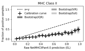 B)
B)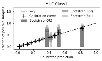
B.3 Generating the calibration function
We use a variant of isotone regression to generate a calibration function as described in Section 3.2. Given a list of triplets , where is raw predicted value of peptide , is the ground truth value of peptide , and is the weight assigned to peptide , ordered such that for all we have , we generate by minimizing the following function, subject to the constraint that and .
| (21) |
Implementation-wise, what we do is to slide a window of size across a list of triplets sorted by prediction outputs to produce a pair of weighted averages of calibrated predictions and weighted averages of ground truth values. For our use case we take to be 1000. We then calculate the squared error and perform projected gradient descent with respect to the squared error over the calibrated weighted predictions. Projection is used to maintain the monotonicity of the calibrated predictions.
This optimization defines over the finite domain of raw predicted values. Let be the set of all raw predicted values. We use the following criterion to extend these predictions to .
| (22) |
While the objective is strictly convex with respect to the averaged values, there are potentially multiple sets of values that produce the same set of averaged values, leading to potentially multiple solutions that optimize Equation 21. We therefore fix the first calibrated predictions to be 0, which is reasonable since it turns out that the first ground truth values are also 0. Having fixed these values, there is now a bijective linear function between the remaining calibrated prediction values and the set of averaged calibration values. Therefore, the objective is also strictly convex with respect to the unaveraged calibrated prediction values.
Appendix C Implementation details
C.1 Computing
To compute in time , it suffices to calculate in time for each since we can then add up all the values.
To calculate in time , we use iterated convolutions. We store a zero indexed list of size initialized such that except for , where we have . Then for each , we loop in reverse order from to and update the list by setting to , where is the credence that is displayed by . is set to . The result is a convolution of a distribution with probability mass function a Bernoulli random variable whose chance of success is . In other words, after each iteration of the loop the value of represents the probability of attaining hits from a vaccine given the peptides that have already been looped over. Performing this loop for all members of then gives the probability distribution for if all random variables in the sum are independent. We can then take the expectation by using the identity . Each loop runs in time , loops need to be run, so computing the distribution takes time overall. If the utility function is provided in some data structure that allows random access (e.g. an array), then the expectation can be computed in time . Thus, can be calculated in time , which gives an overall runtime of for calculating .
C.2 Computing the marginal improvement
Let be fixed, and suppose for some . Then we can calculate in time instead if we store the distribution of for each . This is because we only need to convolve a single Bernoulli random variable over the distribution of to get the distribution of . This then allows us to calculate the expectation in time , which then gives an overall runtime of for calculating the marginal improvement.
At the end of each greedy step, we can update the distributions of to for all in time by performing a single convolution between the distribution and a Bernoulli random variable.
C.3 Vectorization
The calculation of the marginal differences can be vectorized: let be the probability mass function of and let be the probability mass function of . Let be the credence that the element in is displayed on . Let and be represented by vectors where is the probability that the random variable distributed with probability mass function takes on value , and likewise for . Let be a vector representing the utility function, where . Then the expected value of is if is distributed with probability mass function (likewise for ).
If is a vector, let denote a shift operation where and . Let be the reverse operation where and if is the size of . If we ensure that the entry at the last index of is 0 such that and , then the marginal difference is:
| (23) |
This can be rearranged as the following:
| (24) | ||||
| (25) | ||||
| (26) | ||||
| (27) |
Therefore, if we precompute and vectorize , the marginal difference is simply a scaled dot product. This is a vector operation. We can then further tensor over and to parallelize most of the operations.
C.4 Details on hardware, software, and runtime
Our experiments were all run on Titan RTX GPUs, each with 24190MiB of memory. Our algorithms were all implemented in Python 3.7.3 and make use of PyTorch 1.7.1 and Numpy 1.18.5, and were all run on Ubuntu 18.04.3 LTS.
We benchmarked the runtime of Algorithm 1 by generating vaccine designs of size 20 using synthetic datasets where binding credences are drawn uniformly and independently between 0 and 1, with and varying sizes of . 10 runs were excecuted for each . We ran the benchmarks both parallelized over 8 GPUs. We also ran the benchmarks using a single GPU to check how much parallelization over multiple GPUs helps. The runtimes we recorded are given in Figure 6A and 6B.
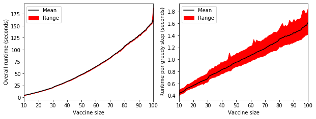
Furthermore, we fixed to , and generated vaccine designs of size between 10 and 100 inclusive. The runtimes are given in Figure 6C.
Appendix D Benchmarking details
D.1 Generating random settings for optimization
We generate 2000 settings in which to benchmark our algorithms against baselines. The number of peptides, the number of genotypes, the genotype weights, the credences assigned to whether a given genotype displays a given peptide, and the optimization objective were all randomized independently and were drawn in the following way:
-
1.
The number of peptides and number of genotypes were drawn uniformly from integers between 512 and 2048 inclusive.
-
2.
All genotype weights were drawn independently and identically from the exponential distribution and then normalized so that they sum to 1. Note that the scale parameter of the distribution is irrelevant since the values are normalized.
-
3.
A value is set to be , where is drawn from the uniform distribution supported between 0 and 1.
-
4.
For each and , is assigned , where the values for are drawn independently and identically from the uniform distribution supported between 0 and 1.
-
5.
The function parametrizing was set to be the following for all integer values:
(28) Where for , the are drawn independently and uniformly from the lognormal distribution with location parameter 0 and scale paramter 2. For simplicity we define if regardless of . This ensures that has decreasing second difference and a non-negative first difference, which in turn ensures that is monotonically increasing and concave (i.e. has monotonically decreasing first differences).
For each setting, designs of size 1-64 inclusive were generated using Algorithm 1. Baseline designs of size 1-64 inclusive were chosen by greedily selecting peptides that were displayed on the most (weighted) genotypes without regards to potentially diminishing returns (linear approximation). A second set of baseline designs were chosen by sampling uniformly at random without replacement to produce a trajectory of 64 designs of size 1-64 inclusive (random). We show in the main body of this work that Algorithm 1 outperforms both approaches (see Figure 2).
We also calculated the amount by which Algorithm 1 outperforms the baseline, which we present in Figure 7. The linear approximation baseline is much more competitive than the random baseline, although Algorithm 1 still outperforms it by more than in some settings.
A)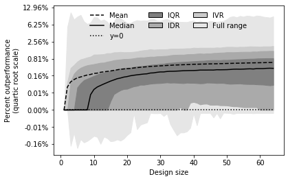 B)
B)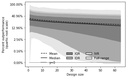
D.2 Analysis of diminishing returns designs on additional utility scores
Figure 3 compares designs generated via the diminishing returns framework against previous designs using . Additional comparisons using , , , and are provided in Figure 8. We similarly observe that the diminishing returns based designs achieve the best performance.
A)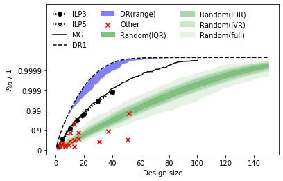 E)
E)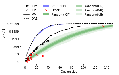 B)
B)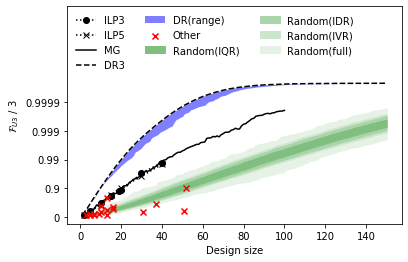 F)
F)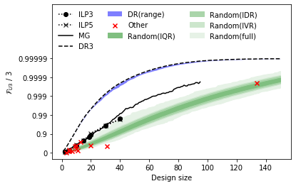 C)
C)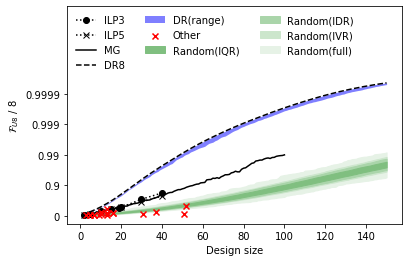 G)
G)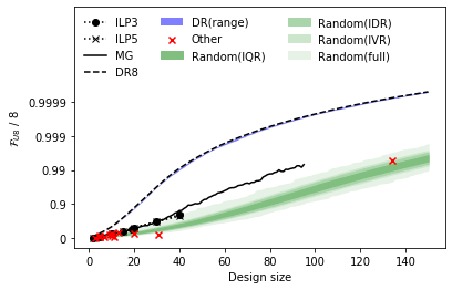 D)
D)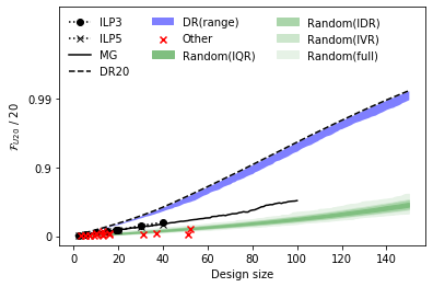 H)
H)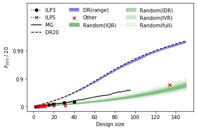
We also provide the scores for the benchmark designs in Table D.2, with comparisons against diminishing returns designs of matching size.
| Peptide vaccine design (MHC1) |
Vaccine size
(number of peptides) |
evaluated on the diminishing returns design of the same size optimized for | |
| \citetAppdxherst2020effective | 52 | 3.76697 | 4.99580 |
| \citetAppdxntimescoverage | 19 | 3.39579 | 4.69175 |
| \citetAppdxntimescoverage | 19 | 3.20910 | 4.69175 |
| \citetAppdxfast2020potential | 13 | 2.93663 | 4.16200 |
| \citetAppdxsrivastava2020structural | 37 | 2.14414 | 4.97735 |
| \citetAppdxporan2020sequence | 10 | 1.80712 | 3.63369 |
| \citetAppdxherst2020effective top16 | 16 | 1.68352 | 4.49048 |
| \citetAppdxahmed2020preliminary | 16 | 1.46971 | 4.49048 |
| \citetAppdxlee2020silico | 13 | 1.34565 | 4.16200 |
| \citetAppdxvashi2020understanding | 51 | 1.12589 | 4.99536 |
| \citetAppdxabdelmageed2020design | 10 | 0.95321 | 3.63369 |
| \citetAppdxakhand2020genome | 31 | 0.91429 | 4.95097 |
| \citetAppdxgupta2020identification | 7 | 0.69957 | 2.82761 |
| \citetAppdxbaruah2020immunoinformatics | 5 | 0.64483 | 2.12411 |
| \citetAppdxmitramulti | 9 | 0.57102 | 3.39366 |
| \citetAppdxalam2020design | 3 | 0.49469 | 1.33187 |
| \citetAppdxsaha2020silico | 5 | 0.48918 | 2.12411 |
| \citetAppdxbhattacharya2020development | 13 | 0.41408 | 4.16200 |
| \citetAppdxsingh2020designing | 7 | 0.40922 | 2.82761 |
| Peptide vaccine design (MHC2) |
Vaccine size
(number of peptides) |
evaluated on the diminishing returns design of the same size optimized for | |
| \citetAppdxramaiah2021insights | 134 | 4.99516 | 4.99988 |
| \citetAppdxntimescoverage | 19 | 3.28835 | 4.69175 |
| \citetAppdxntimescoverage | 19 | 3.25892 | 4.69175 |
| \citetAppdxfast2020potential | 13 | 2.54511 | 4.16200 |
| \citetAppdxvashi2020understanding | 20 | 1.95264 | 4.73921 |
| \citetAppdxabdelmageed2020design | 10 | 1.90814 | 3.63369 |
| \citetAppdxakhand2020genome | 31 | 1.72526 | 4.95097 |
| \citetAppdxbanerjee2020energetics | 9 | 1.71810 | 3.39366 |
| \citetAppdxporan2020sequence | 10 | 1.10991 | 3.63369 |
| \citetAppdxmitramulti | 5 | 0.96545 | 2.12411 |
| \citetAppdxtahir2020designing | 11 | 0.77791 | 3.83742 |
| \citetAppdxahmed2020preliminary | 5 | 0.55950 | 2.12411 |
| \citetAppdxsingh2020designing | 7 | 0.40133 | 2.82761 |
| \citetAppdxbaruah2020immunoinformatics | 3 | 0.00000 | 1.33187 |
D.3 Comparison of designs using n-times coverage
We compare the performance of vaccines with 19 peptides designed from the diminishing returns framework against vaccines with 19 peptides from \citetAppdxntimescoverage in Figure 4. We additionally compare the performance of designs of varying sizes in Figure 9. The credences used in the objective for optimizing the diminishing returns designs were binarized to closely match the binding data used by \citetAppdxntimescoverage, while the -times coverage evaluation was reproduced from \citetAppdxntimescoverage.
Similarly to our analysis from Figure 4, we find that diminishing returns designs are highly competitive even when evaluated on the -times coverage objective. We find that this is especially the case for designs for Class II MHCs, where prior approaches appear to get stuck at a certain thresholds.
A)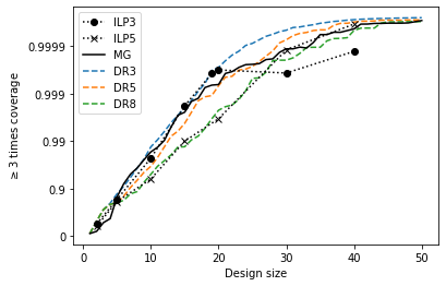 D)
D)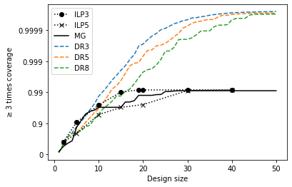 B)
B)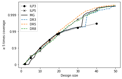 E)
E)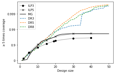 C)
C)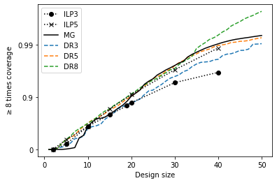 F)
F)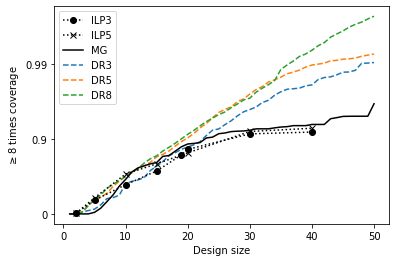
plainnat \bibliographyAppdxreferences