Maximum Likelihood Training for Score-Based Diffusion ODEs
by High-Order Denoising Score Matching
Abstract
Score-based generative models have excellent performance in terms of generation quality and likelihood. They model the data distribution by matching a parameterized score network with first-order data score functions. The score network can be used to define an ODE (“score-based diffusion ODE”) for exact likelihood evaluation. However, the relationship between the likelihood of the ODE and the score matching objective is unclear. In this work, we prove that matching the first-order score is not sufficient to maximize the likelihood of the ODE, by showing a gap between the maximum likelihood and score matching objectives. To fill up this gap, we show that the negative likelihood of the ODE can be bounded by controlling the first, second, and third-order score matching errors; and we further present a novel high-order denoising score matching method to enable maximum likelihood training of score-based diffusion ODEs. Our algorithm guarantees that the higher-order matching error is bounded by the training error and the lower-order errors. We empirically observe that by high-order score matching, score-based diffusion ODEs achieve better likelihood on both synthetic data and CIFAR-10, while retaining the high generation quality.
1 Introduction

(a) Data
(b) ScoreODE
(first-order SM)
(c) ScoreODE
(third-order SM)
Score-based generative models (SGMs) have shown promising performance in both sample quality and likelihood evaluation (Song et al., 2020b; Vahdat et al., 2021; Dockhorn et al., 2021; Kingma et al., 2021), with applications on many tasks, such as image generation (Dhariwal & Nichol, 2021; Meng et al., 2021b), speech synthesis (Chen et al., 2020; Kong et al., 2020), shape generation (Luo & Hu, 2021; Zhou et al., 2021) and lossless compression (Kingma et al., 2021). SGMs define a forward diffusion process by a stochastic differential equation (SDE) that gradually perturbs the data distribution to a simple noise distribution. The forward diffusion process has an equivalent reverse-time process with analytical form (Anderson, 1982), which depends on the score function (the gradient of the log probability density) of the forward process at each time step. SGMs learn a parameterized neural network (called “score model”) (Song et al., 2020a; Song & Ermon, 2019, 2020; Song et al., 2020b) to estimate the score functions, and further define probabilistic models by the score model.
Two types of probabilistic models are proposed with the learned score model. One is the score-based diffusion SDE (Song et al. (2020b), “ScoreSDE” for short), which is defined by approximately reversing the diffusion process from the noise distribution by the score model and it can generate high-quality samples. The other is the score-based diffusion ordinary differential equation (Song et al. (2020b, 2021), “ScoreODE” for short), which is defined by approximating the probability flow ODE (Song et al., 2020b) of the forward process whose marginal distribution is the same as the forward process at each time. ScoreODEs can be viewed as continuous normalizing flows (Chen et al., 2018). Thus, unlikely SDEs, they can compute exact likelihood by ODE solvers (Grathwohl et al., 2018).
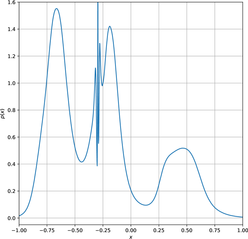
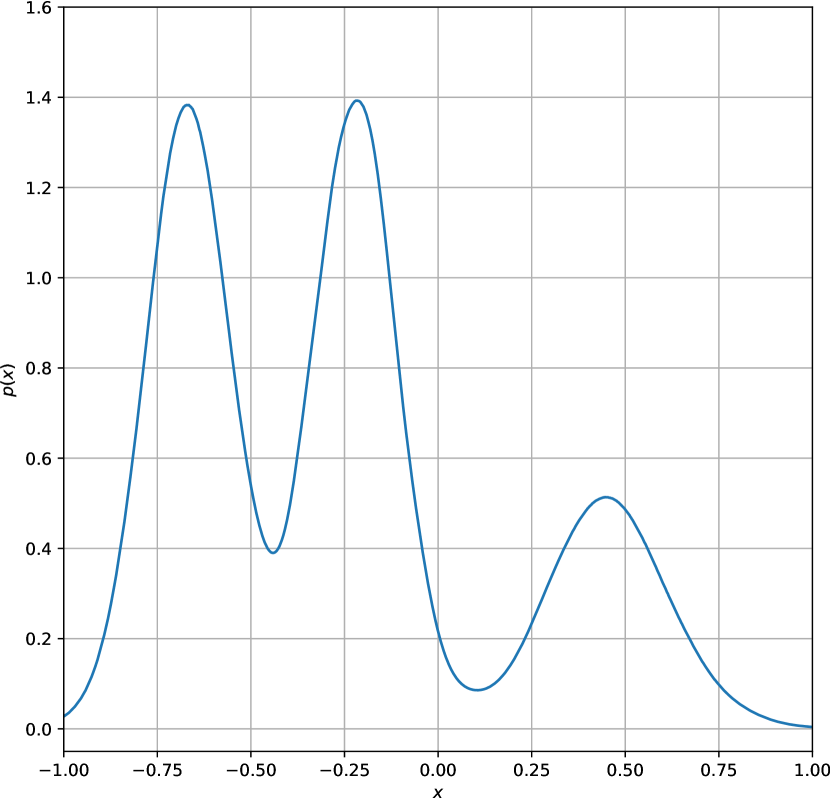
In practice, the score models are trained by minimizing an objective of a time-weighted combination of score matching losses (Hyvärinen & Dayan, 2005; Vincent, 2011). It is proven that for a specific weighting function, minimizing the score matching objective is equivalent to maximizing the likelihood of the ScoreSDE (Song et al., 2021). However, minimizing the score matching objective does not necessarily maximize the likelihood of the ScoreODE. This is problematic since ScoreODEs are used for likelihood estimation. In fact, ScoreODEs trained with the score matching objective may even fail to estimate the likelihood of very simple data distributions, as shown in Fig. 1.
In this paper, we systematically analyze the relationship between the score matching objective and the maximum likelihood objective of ScoreODEs, and present a new algorithm to learn ScoreODEs via maximizing likelihood. Theoretically, we derive an equivalent form of the KL divergence111Maximum likelihood estimation is equivalent to minimizing a KL divergence. between the data distribution and the ScoreODE distribution, which explicitly reveals the gap between the KL divergence and the original first-order score matching objective. Computationally, as directly optimizing the equivalent form requires an ODE solver, which is time-consuming (Chen et al., 2018), we derive an upper bound of the KL divergence by controlling the approximation errors of the first, second, and third-order score matching. The optimal solution for this score model by minimizing the upper bound is still the data score function, so the learned score model can still be used for the sample methods in SGMs (such as PC samplers in (Song et al., 2020b)) to generate high-quality samples.
Based on the analyses, we propose a novel high-order denoising score matching algorithm to train the score models, which theoretically guarantees bounded approximation errors of high-order score matching. We further propose some scale-up techniques for practice. Our experimental results empirically show that the proposed training method can improve the likelihood of ScoreODEs on both synthetic data and CIFAR-10, while retaining the high generation quality.
2 Score-Based Generative Models
We first review the dynamics and probability distributions defined by SGMs. The relationship between these dynamics is illustrated in Fig. 2(a).
2.1 ScoreSDEs and Maximum Likelihood Training
Let denote an unknown -dimensional data distribution. SGMs define an SDE from time to (called “forward process”) with and
| (1) |
where is the solution at time , and are fixed functions such that the marginal distribution of is approximately with , and is the standard Wiener process. Let denote the marginal distribution of . Under some regularity conditions, the forward process in Eqn. (1) has an equivalent reverse process (Anderson, 1982) from time to with :
| (2) |
where is a standard Wiener process in the reverse-time. The marginal distribution of in the reverse process in Eqn. (2) is also . The only unknown term in Eqn. (2) is the time-dependent score function . SGMs use a neural network parameterized by to estimate the score function for all and . The neural network is trained by matching and with the score matching objective:
where is a weighting function. By approximating the score function with , SGMs define a parameterized reverse SDE from time to time with probability at each time denoted as (omitting the subscript ). In particular, suppose , the parameterized reverse SDE is defined by
| (3) |
where the marginal distribution of is . By solving the parameterized reverse SDE, SGMs achieve excellent sample quality in many tasks (Song et al., 2020b; Dhariwal & Nichol, 2021). Moreover, the KL divergence between and can be bounded by the score matching error with the weight (Song et al., 2021):
| (4) |
Therefore, minimizing is equivalent to maximum likelihood training of . In the rest of this work, we mainly consider the maximum likelihood perspective, namely , and denote .
2.2 ScoreODEs and Exact Likelihood Evaluation
The parameterized ScoreSDE cannot be used for exact likelihood evaluation, because we cannot evaluate exactly for a given point . However, every SDE has an associated probability flow ODE (Song et al., 2020b) whose marginal distribution at each time is the same as that of the SDE. Unlike SDEs, the log-density of the ODE can be exactly computed by the “Instantaneous Change of Variables” (Chen et al., 2018). Particularly, the probability flow ODE of the forward process in Eqn. (1) is
| (5) |
If we start from , the distribution of each during the ODE trajectory is also . Note that the only unknown term in Eqn. (5) is also the score function . By approximating the score function with , SGMs define a parameterized ODE called “score-based diffusion ODE” (ScoreODE) with probability (omitting the subscript ) at each time . In particular, suppose , the ScoreODE is defined by
| (6) |
where the marginal distribution of is . By the “Instantaneous Change of Variables” (Chen et al., 2018), of can be computed by integrating:
| (7) |
If for all and , we have . In this case, for all , (because ), where is the point at time given by Eqn. (5) starting with at time . Inspired by this, SGMs use the ScoreODE with the score model for exact likelihood evaluations.
However, if , there is no theoretical guarantee for bounding of ScoreODEs by the score matching objective . As a result, after minimizing , Song et al. (2021) find that the ScoreSDE of the “Variance Exploding” type (Song et al., 2020b) achieves state-of-the-art sample quality, but the log-likelihood of the corresponding ScoreODE is much worse (e.g., bits/dim on CIFAR-10 dataset) than that of other comparable models (e.g., bits/dim of the ”Variance Preserving” type (Song et al., 2020b)). Such observations pose a serious concern on the behavior of the likelihood of , which is not well understood. We aim to provide a systematical analysis in this work.
3 Relationship between Score Matching and KL Divergence of ScoreODEs
(a) Relationship between , and .
(b) Relationship between SM objectives and KL divergence.
The likelihood evaluation needs the distribution of ScoreODEs, which is usually different from the distribution of ScoreSDEs (see Appendix B for detailed discussions). Although the score matching objective can upper bound the KL divergence of ScoreSDEs (up to constants) according to Eqn. (4), it is not enough to upper bound the KL divergence of ScoreODEs. To the best of our knowledge, there is no theoretical analysis of the relationship between the score matching objectives and the KL divergence of ScoreODEs.
In this section, we reveal the relationship between the first-order score matching objective and the KL divergence of ScoreODEs, and upper bound by involving high-order score matching. Fig. 2 demonstrates our theoretical analysis and the connection with previous works.
3.1 KL Divergence of ScoreODEs
In the following theorem, we propose a formulation of the KL divergence by integration, which shows that there is a non-zero gap between the KL divergence and the score matching objective .
Theorem 3.1 (Proof in Appendix E.1).
As is fixed, minimizing is equivalent to minimizing , which includes and . While minimizing reduces the difference between and the data score , it cannot control the error of , which includes the difference between and the model score . As we show in Fig. 1, only minimizing may cause problematic model density of the ScoreODE.
3.2 Bounding the KL Divergence of ScoreODEs by High-Order Score Matching Errors
The KL divergence in Theorem 3.1 includes the model score function , which needs ODE solvers to compute (see Appendix. D for details) and thus is hard to scale up. Below we derive an upper bound of by involving high-order score matching, which can avoid the computation of . Specifically, we show that by bounding the first, second and third-order score matching errors for and with the corresponding order score functions222In this work, we refer to as the second-order score function of , and as the third-order score function of . of , we can further upper bound .
Let denote the Fisher divergence between two distributions and . Define
| (10) |
By straightforwardly using Cauchy-Schwarz inequality for Eqn. (8), we have
| (11) |
The upper bound shows that we can minimize the KL divergence of ScoreODE by minimizing and simultaneously. When for all and , the equality holds and .
We can regard as a weighted Fisher divergence between and during . Directly computing the Fisher divergence also needs ODE solvers (see Appendix.D for details) and is hard to scale up. To address this problem, we present the following theorem for bounding , which introduces high-order score matching and avoids the computation costs of ODE solvers.
Theorem 3.2 (Proof in Appendix E.2).
Assume that there exists , such that for all and , (where denotes the second-order derivative (Hessian), and is the spectral norm of a matrix). And assume that there exist , such that for all , , satisfies
where is the Frobenius norm of matrices. Then there exists which depends on the forward process while is independent of , such that . Moreover, for all , if , then is a strictly increasing function of , and , respectively.
Theorem 3.2 shows that by bounding the errors between , and with the first, second and third-order score functions of , we can upper bound and then upper bound . As can also be upper bounded by the first-order score matching error of , we can further upper bound by the first, second and third-order score matching errors.
Note that the high-order score matching for is compatible for the traditional SGMs, because the optimal solution for in the non-parametric limit is still . So after minimizing by high-order score matching, we can still use for the sample methods in SGMs, while directly minimizing by exact likelihood ODE solvers cannot ensure that (see Appendix. E.3 for detailed reasons).
4 Error-Bounded High-Order Denoising Score Matching (DSM)
The analysis in Sec. 3.2 shows that we can upper bound the KL divergence of the ScoreODE by controlling the first, second and third-order score matching errors of the score model (and its corresponding derivatives) at each time . Inspired by this, we generalize the traditional denoising score matching (DSM) (Vincent, 2011) to second and third orders to minimize the high-order score matching errors. In this section, we propose a novel high-order DSM method, such that the higher-order score matching error can be exactly bounded by the training error and the lower-order score matching error. All the proofs in this section are in Appendix. F.
Without loss of generality, in this section, we focus on a fixed time , and propose the error-bounded high-order DSM method for matching the forward process distribution at the fixed time . The whole training objective for the entire process by is detailed in Sec. 5. Moreover, for SGMs, there commonly exist and , such that the forward process satisfies for (Song et al., 2020b). Therefore, we always assume in the rest of this work.
4.1 First-Order Denoising Score Matching
We present some preliminaries on first-order denoising score matching (Vincent, 2011; Song et al., 2020b) in this section.
The first-order score matching objective needs the data score functions for all , which are unknown in practice. To address this issue, SGMs leverage the denoising score matching method (Vincent, 2011) to train the score models. For a fixed time , one can learn a first-order score model parameterized by which minimizes
by optimizing the (first-order) DSM objective:
| (12) |
where and .
4.2 High-Order Denoising Score Matching
In this section, we generalize the first-order DSM to second and third orders for matching the second-order and third-order score functions defined in Theorem 3.2. We firstly present the second-order method below.
Theorem 4.1.
(Error-Bounded Second-Order DSM) Suppose that is an estimation for the first-order data score function , then we can learn a second-order score model parameterized by which minimizes
by optimizing
| (13) |
where
| (14) | ||||
Moreover, denote the first-order score matching error as , then , the score matching error for can be bounded by
Theorem 4.1 shows that the DSM objective in problem (13) is a valid surrogate for second-order score matching, because the difference between the model score and the true second-order score can be bounded by the training error and the first-order score matching error . Note that previous second-order DSM method proposed in Meng et al. (2021a) does not have such error-bounded property, and we refer to Sec. 6 and Appendix F.4 for the detailed comparison. In addition, recent work (Bao et al., 2022, Theorem 3.3) about the optimal covariance of the diffusion models considers the estimation error of the mean of the diffusion models, which is equivalent to our proposed error-bounded second-order DSM with considering the first-order score matching error.
The DSM objective in problem (13) requires learning a matrix-valued function , but sometimes we only need the trace of the second-order score function. Below we present a corollary for only matching the trace of the second-order score function.
Corollary 4.2.
(Error-Bounded Trace of Second-Order DSM) We can learn a second-order trace score model which minimizes
by optimizing
| (15) |
The estimation error for can be bounded by:
Finally, we present the third-order DSM method. The score matching error can also be bounded by the training error and the first, second-order score matching errors.
Theorem 4.3.
(Error-Bounded Third-Order DSM) Suppose that is an estimation for and is an estimation for , then we can learn a third-order score model which minimizes
by optimizing
| (16) |
where
| (17) |
Denote the first-order score matching error as and the second-order score matching errors as and . Then , the score matching error for can be bounded by:
Theorem 4.3 shows that the third-order score matching needs first-order score matching, second-order score matching and trace of second-order score matching. The third-order score matching error can also be bounded by the training error and the lower-order score matching errors. We believe that our construction for the error-bounded high-order DSM can be extended to even higher orders by carefully designing the training objectives. In this paper, we only focus on the second and third-order methods, and leave this extension for future work.
5 Training Score Models by High-Order DSM
Building upon the high-order DSM for a specific time (see Sec. 4), we present our algorithm to train ScoreODEs in the perspective of maximum likelihood by considering all timesteps . Practically, we further leverage the “noise-prediction” trick (Kingma et al., 2021; Ho et al., 2020) for variance reduction and the Skilling-Hutchinson trace estimator (Skilling, 1989; Hutchinson, 1989) to compute the involved high-order derivatives efficiently. The whole training algorithm is presented detailedly in Appendix. H.
5.1 Variance Reduction by Time-Reweighting
Theoretically, to train score models for all , we need to integrate the DSM objectives in Eqn. (12)(13)(15)(16) from to , which needs ODE solvers and is time-consuming. Instead, in practice, we follow the method in (Song et al., 2020b; Ho et al., 2020) which uses Monte-Carlo method to unbiasedly estimate the objectives by sample from a proposal distribution , avoiding ODE solvers. The main problem for the Monte-Carlo method is that sometimes the sample variance of the objectives may be large due to the different value of . To reduce the variance, we take the time-reweighted objectives by multiplying ,, with the corresponding first, second, third-order score matching objectives at each time , which is known as the “noise-prediction” trick (Kingma et al., 2021; Ho et al., 2020) for the first-order DSM objective. Specifically, assume that , the time proposal distribution is the uniform distribution in , the random noise follows the standard Gaussian distribution, and let . The training objective for the first-order DSM in Eqn. (12) through all is
| (18) |
which empirically has low sample variance (Song et al., 2020b; Ho et al., 2020).
As for the second and third-order DSM objectives, we take for the first-order score function estimation, and for the second-order score function estimation, and both disable the gradient computations for (which can be easily implemented by stop_gradient or detach). The reason for disabling gradients is because the high-order DSM only needs the estimation values of the lower-order score functions, as shown in Theorem. 4.1 and 4.3. The training objectives through all for the second-order DSM in Eqn. (13), for the trace of second-order DSM in Eqn. (15) and for the third-order DSM in Eqn. (16) are
respectively, where are the same as that in Eqn. (17). Combining with the first-order objective in Eqn. (18), our final training objective is
| (19) |
where are hyperparameters, and we discuss in Appendix. I.1 for details.
Remark.
Although as shown in Eqn. (7), we can exactly compute for a given data point via solving the ODE (Chen et al., 2018; Grathwohl et al., 2018), this method is hard to scale up for the large neural networks used in SGMs. For example, it takes minutes for evaluating for a single batch of the ScoreODE used in (Song et al., 2020b). Instead, our proposed method leverages Monte-Carlo methods to avoid the ODE solvers.
5.2 Scalability and Numerical Stability
As the second and third-order DSM objectives need to compute the high-order derivatives of a neural network and are expensive for high-dimensional data, we use the Skilling-Hutchinson trace estimator (Skilling, 1989; Hutchinson, 1989) to unbiasedly estimate the trace of the Jacobian (Grathwohl et al., 2018) and the Frobenius norm of the Jacobian (Finlay et al., 2020). The detailed objectives for high-dimensional data can be found in Appendix. G.
In practice, we often face numerical instability problems for near to . We follow Song et al. (2021) to choose a small starting time , and both of the training and the evaluation are performed for instead of . Note that the likelihood evaluation is still exact, because we use to compute the log-likelihood of , which is still a well-defined density model (Song et al., 2021).
6 Related Work
ScoreODEs are special formulations of Neural ODEs (NODEs) (Chen et al., 2018), and our proposed method can be viewed as maximum likelihood training of NODEs by high-order score matching. Traditional maximum likelihood training for NODEs aims to match the NODE distribution at with the data distribution, and it cannot control the distribution between and . Finlay et al. (2020) show that training NODEs by simply maximizing likelihood could result in unnecessary complex dynamics, which is hard to solve. Instead, our high-order score matching objective is to match the distributions between the forward process distribution and the NODE distribution at each time , and empirically the dynamics is kind of smooth. Moreover, our proposed algorithm uses the Monto-Carlo method to unbiasedly estimate the objectives, which does not need any black-box ODE solvers. Therefore, our algorithm is suitable for maximum likelihood training for large-scale NODEs.
Recently, Meng et al. (2021a) propose a high-order DSM method for estimating the second-order data score functions. However, the training objective of our proposed error-bounded high-order DSM is different from that of Meng et al. (2021a). Our proposed algorithm can guarantee a bounded error of the high-order score matching exactly by the lower-order estimation errors and the training error, while the score matching error raised by minimizing the objective in Meng et al. (2021a) may be unbounded, even when the lower-order score matching error is small and the training error of the high-order DSM is zero (see Appendix F.4 for detailed analysis). Moreover, our method can also be used to train a separate high-order score model in other applications, such as uncertainty quantification and Ozaki sampling presented in Meng et al. (2021a).
7 Experiments
In this section, we demonstrate that our proposed high-order DSM algorithm can improve the likelihood of ScoreODEs, while retaining the high sample quality of the corresponding ScoreSDEs. Particularly, we use the Variance Exploding (VE) (Song et al., 2020b) type diffusion models, which empirically have shown high sample quality by the ScoreSDE but poor likelihood by the ScoreODE (Song et al., 2021) when trained by minimizing the first-order score matching objective . We implement our experiments by JAX (Bradbury et al., 2018), which is efficient for computing the derivatives of the score models. In all experiments, we choose the start time , which follows the default settings in Song et al. (2020b). In this section, we refer to “first-order score matching” as minimizing the objective in Eqn. (19) with , and “second-order score matching” as minimizing the one with . Please see Appendix. I.1 for detailed settings about and . The released code can be found at https://github.com/LuChengTHU/mle_score_ode.
Remark.
(a) First-order score matching
(b) Second-order score matching
(c) Third-order score matching
7.1 Example: 1-D Mixture of Gaussians
We take an example to demonstrate how the high-order score matching training impacts the weighted Fisher divergence and the model density of ScoreODEs. Let be a 1-D Gaussian mixture distribution as shown in Fig. 1 (a). We train a score model of VE type by minimizing the first-order score matching objective , and use the corresponding ScoreODE to evaluate the model density, as shown in Fig. 1 (b). The model density achieved by only first-order score matching is quite different from the data distribution at some data points. However, by third-order score matching, the model density in Fig. 1 (c) is quite similar to the data distribution, showing the effectiveness of our proposed algorithm.
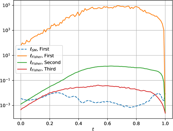
We further analyze the difference of between the first, second, third-order score matching training. As is a Gaussian mixture distribution, we can prove that each is also a Gaussian mixture distribution, and can be analytically computed. Denote
which are the integrands of each time for and . We use the method in Appendix. D to compute , and evaluate and from to with points of the ScoreODEs trained by first, second, third-order denoising score matching objectives. As shown in Fig. 3, although is small when minimizing first-order score matching objective, is rather large for most , which means is also large. However, the second and third score matching gradually reduce , which shows that high-order score matching training can reduce and then reduce . Such results empirically validate that controlling the high-order score matching error can control the Fisher divergence, as proposed in Theorem 3.2.
7.2 Density Modeling on 2-D Checkerboard Data
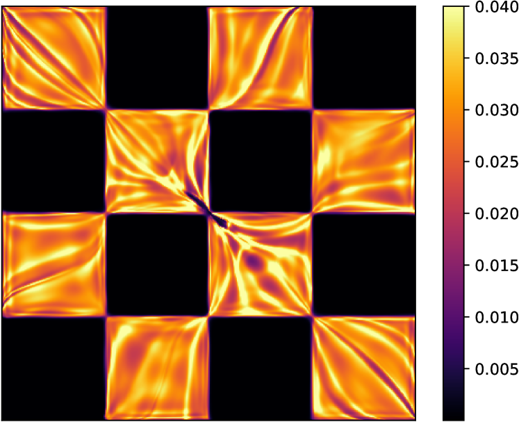
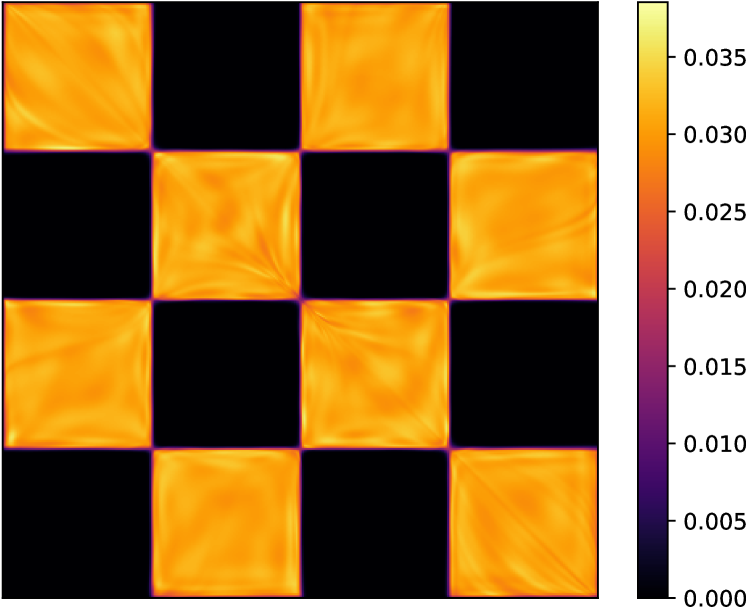
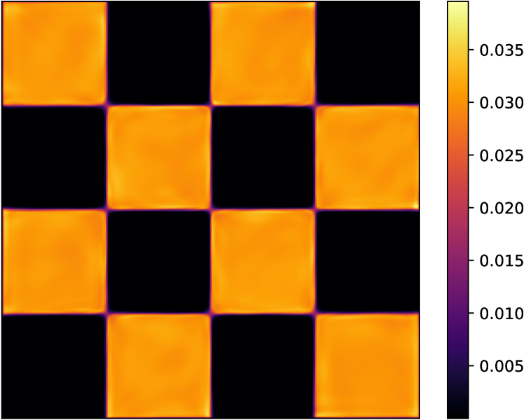
We then train ScoreODEs (VE type) by the first, second, third-order score matchings on the checkerboard data whose density is multi-modal, as shown in Fig. 4. We use a simple MLP neural network with Swish activations (Ramachandran et al., 2017), and the detailed settings are in Appendix. I.3.
For the second and third-order score matchings, we do not use any pre-trained lower-order score models. Instead, we train the score model and its first, second-order derivatives from scratch, using the objective in Eqn. (19). The model density by the first-order score matching is rather poor, because it cannot control the value of in in Eqn. (9). The second-order score matching can control part of and improve the model density, while the third-order score matching can reduce the Fisher divergence and achieve excellent model density. Such results show the effectiveness of our error-bounded high-order denoising score matching methods, and accord with our theoretical analysis in Theorem 3.1 and 3.2.
7.3 Density Modeling on Image Datasets
We also train ScoreODEs (VE type) on both the CIFAR-10 dataset (Krizhevsky, 2009) and the ImageNet 32x32 dataset (Deng et al., 2009), which are two of the most popular datasets for generative modeling and likelihood evaluation. We use the estimated training objectives by trace estimators, which are detailed in Appendix. G. We use the same neural networks and hyperparameters as the NCSN++ cont. model in (Song et al., 2020b) (denoted as VE) and the NCSN++ cont. deep model in (Song et al., 2020b) (denoted as VE (deep)), respectively (see detailed settings in Appendix. I.4 and Appendix. I.5). We evaluate the likelihood by the ScoreODE , and sample from the ScoreSDE by the PC sampler (Song et al., 2020b). As shown in Table 1, our proposed high-order score matching can improve the likelihood performance of ScoreODEs, while retraining the high sample quality of the corresponding ScoreSDEs (see Appendix. J for samples). Moreover, the computation costs of the high-order DSM objectives are acceptable because of the trace estimators and the efficient “Jacobian-vector-product” computation in JAX. We list the detailed computation costs in Appendix. I.4.
We also compare the VE, VP and subVP types of ScoreODEs trained by the first-order DSM and the third-order DSM, and the detailed results are listed in Appendix. J.
8 Conclusion
We propose maximum likelihood training for ScoreODEs by novel high-order denoising score matching methods. We analyze the relationship between the score matching objectives and the KL divergence from the data distribution to the ScoreODE distribution. Based on it, we provide an upper bound of the KL divergence, which can be controlled by minimizing the first, second, and third-order score matching errors of score models. To minimize the high-order score matching errors, we further propose a high-order DSM algorithm, such that the higher-order score matching error can be bounded by exactly the training error and the lower-order score matching errors. The optimal solution for the score model is still the same as the original training objective of SGMs. Empirically, our method can greatly improve the model density of ScoreODEs of the Variance Exploding type on several density modeling benchmarks. Finally, we believe that our training method is also suitable for other SGMs, including the Variance Preserving (VP) type (Song et al., 2020b), the latent space type (Vahdat et al., 2021) and the critically-damped Langevin diffusion type (Dockhorn et al., 2021). Such extensions are left for future work.
Acknowledgements
This work was supported by National Key Research and Development Project of China (No. 2021ZD0110502); NSF of China Projects (Nos. 62061136001, 61620106010, 62076145, U19B2034, U1811461, U19A2081, 6197222, 62106120); Beijing NSF Project (No. JQ19016); Beijing Outstanding Young Scientist Program NO. BJJWZYJH012019100020098; a grant from Tsinghua Institute for Guo Qiang; the NVIDIA NVAIL Program with GPU/DGX Acceleration; the High Performance Computing Center, Tsinghua University; and Major Innovation & Planning Interdisciplinary Platform for the “Double-First Class” Initiative, Renmin University of China.
References
- Anderson (1982) Anderson, B. D. Reverse-time diffusion equation models. Stochastic Processes and their Applications, 12(3):313–326, 1982.
- Bao et al. (2022) Bao, F., Li, C., Sun, J., Zhu, J., and Zhang, B. Estimating the optimal covariance with imperfect mean in diffusion probabilistic models. arXiv preprint arXiv:2206.07309, 2022.
- Bradbury et al. (2018) Bradbury, J., Frostig, R., Hawkins, P., Johnson, M. J., Leary, C., Maclaurin, D., Necula, G., Paszke, A., VanderPlas, J., Wanderman-Milne, S., and Zhang, Q. JAX: Composable transformations of Python+NumPy programs, 2018. URL http://github.com/google/jax.
- Chen et al. (2020) Chen, N., Zhang, Y., Zen, H., Weiss, R. J., Norouzi, M., and Chan, W. Wavegrad: Estimating gradients for waveform generation. arXiv preprint arXiv:2009.00713, 2020.
- Chen et al. (2018) Chen, R. T., Rubanova, Y., Bettencourt, J., and Duvenaud, D. Neural ordinary differential equations. arXiv preprint arXiv:1806.07366, 2018.
- Deng et al. (2009) Deng, J., Dong, W., Socher, R., Li, L., Li, K., and Fei-Fei, L. ImageNet: A large-scale hierarchical image database. In 2009 IEEE Conference on Computer Vision and Pattern Recognition, pp. 248–255. IEEE, 2009.
- Dhariwal & Nichol (2021) Dhariwal, P. and Nichol, A. Diffusion models beat GANs on image synthesis. arXiv preprint arXiv:2105.05233, 2021.
- Dockhorn et al. (2021) Dockhorn, T., Vahdat, A., and Kreis, K. Score-based generative modeling with critically-damped langevin diffusion. arXiv preprint arXiv:2112.07068, 2021.
- Finlay et al. (2020) Finlay, C., Jacobsen, J.-H., Nurbekyan, L., and Oberman, A. How to train your Neural ODE: the world of Jacobian and kinetic regularization. In International Conference on Machine Learning, pp. 3154–3164. PMLR, 2020.
- Grathwohl et al. (2018) Grathwohl, W., Chen, R. T., Bettencourt, J., Sutskever, I., and Duvenaud, D. FFJORD: Free-form continuous dynamics for scalable reversible generative models. arXiv preprint arXiv:1810.01367, 2018.
- Ho et al. (2020) Ho, J., Jain, A., and Abbeel, P. Denoising diffusion probabilistic models. arXiv preprint arXiv:2006.11239, 2020.
- Huang et al. (2021) Huang, C.-W., Lim, J. H., and Courville, A. A variational perspective on diffusion-based generative models and score matching. arXiv preprint arXiv:2106.02808, 2021.
- Hutchinson (1989) Hutchinson, M. F. A stochastic estimator of the trace of the influence matrix for Laplacian smoothing splines. Communications in Statistics-Simulation and Computation, 18(3):1059–1076, 1989.
- Hyvärinen & Dayan (2005) Hyvärinen, A. and Dayan, P. Estimation of non-normalized statistical models by score matching. Journal of Machine Learning Research, 6(4), 2005.
- Kingma & Ba (2014) Kingma, D. P. and Ba, J. Adam: A method for stochastic optimization. arXiv preprint arXiv:1412.6980, 2014.
- Kingma et al. (2021) Kingma, D. P., Salimans, T., Poole, B., and Ho, J. Variational diffusion models. arXiv preprint arXiv:2107.00630, 2021.
- Kong et al. (2020) Kong, Z., Ping, W., Huang, J., Zhao, K., and Catanzaro, B. Diffwave: A versatile diffusion model for audio synthesis. arXiv preprint arXiv:2009.09761, 2020.
- Krizhevsky (2009) Krizhevsky, A. Learning multiple layers of features from tiny images. Technical report, 2009.
- Luo & Hu (2021) Luo, S. and Hu, W. Diffusion probabilistic models for 3D point cloud generation. In Proceedings of the IEEE/CVF Conference on Computer Vision and Pattern Recognition, pp. 2837–2845, 2021.
- Meng et al. (2021a) Meng, C., Song, Y., Li, W., and Ermon, S. Estimating high order gradients of the data distribution by denoising. Advances in Neural Information Processing Systems, 34, 2021a.
- Meng et al. (2021b) Meng, C., Song, Y., Song, J., Wu, J., Zhu, J.-Y., and Ermon, S. SDEdit: Image synthesis and editing with stochastic differential equations. arXiv preprint arXiv:2108.01073, 2021b.
- Ramachandran et al. (2017) Ramachandran, P., Zoph, B., and Le, Q. V. Searching for activation functions. arXiv preprint arXiv:1710.05941, 2017.
- Skilling (1989) Skilling, J. The eigenvalues of mega-dimensional matrices. In Maximum Entropy and Bayesian Methods, pp. 455–466. Springer, 1989.
- Song & Ermon (2019) Song, Y. and Ermon, S. Generative modeling by estimating gradients of the data distribution. arXiv preprint arXiv:1907.05600, 2019.
- Song & Ermon (2020) Song, Y. and Ermon, S. Improved techniques for training score-based generative models. arXiv preprint arXiv:2006.09011, 2020.
- Song et al. (2020a) Song, Y., Garg, S., Shi, J., and Ermon, S. Sliced score matching: A scalable approach to density and score estimation. In Uncertainty in Artificial Intelligence, pp. 574–584. PMLR, 2020a.
- Song et al. (2020b) Song, Y., Sohl-Dickstein, J., Kingma, D. P., Kumar, A., Ermon, S., and Poole, B. Score-based generative modeling through stochastic differential equations. arXiv preprint arXiv:2011.13456, 2020b.
- Song et al. (2021) Song, Y., Durkan, C., Murray, I., and Ermon, S. Maximum likelihood training of score-based diffusion models. arXiv e-prints, pp. arXiv–2101, 2021.
- Vahdat et al. (2021) Vahdat, A., Kreis, K., and Kautz, J. Score-based generative modeling in latent space. arXiv preprint arXiv:2106.05931, 2021.
- Vincent (2011) Vincent, P. A connection between score matching and denoising autoencoders. Neural computation, 23(7):1661–1674, 2011.
- Zhou et al. (2021) Zhou, L., Du, Y., and Wu, J. 3D shape generation and completion through point-voxel diffusion. arXiv preprint arXiv:2104.03670, 2021.
Appendix A Assumptions
We follow the regularity assumptions in (Song et al., 2021) to ensure the existence of reverse-time SDEs and probability flow ODEs and the correctness of the “integration by parts” tricks for the computation of KL divergence. And to ensure the existence of the third score function, we change the assumptions of differentiability. For completeness, we list all these assumptions in this section.
For simplicity, in the Appendix sections, we use to denote and omit the subscript . And we denote as the divergence of a function .
Assumption A.1.
We make the following assumptions, most of which are presented in (Song et al., 2021):
-
1.
and .
-
2.
. And , .
-
3.
.
-
4.
and .
-
5.
For any open bounded set , .
-
6.
.
-
7.
.
-
8.
.
-
9.
.
-
10.
Novikov’s condition: .
-
11.
, , as .
Appendix B Distribution gap between score-based diffusion SDEs and ODEs
| Distribution | Dynamics type | Formulation |
|---|---|---|
| Forward SDE | ||
| Reverse SDE | ||
| Probability flow ODE | ||
| Forward SDE | ||
| Reverse SDE | ||
| Probability flow ODE | ||
| Forward SDE | ||
| Reverse SDE | ||
| Probability flow ODE |
We list the corresponding equivalent SDEs and ODEs of , and in Table 2. In most cases, , and are different distributions, which we will prove in this section.
According to the reverse SDE and probability flow ODE listed in the table, it is obvious that when , and are different, and , are different. Below we show that in most cases, and are also different.
Firstly, we should notice that the probability flow ODE of the ScoreSDE in Eqn. (3) is
| (20) |
where the distribution of during the trajectory is also . Below we show that for the commonly-used SGMs, in most cases, the probability flow ODE in Eqn. (20) of the ScoreSDE is different from the ScoreODE in Eqn. (6).
Proposition B.1.
Assume is a linear function of for all and , where . If for all and , , then is a Gaussian distribution for all .
Proof.
If , then for any , by Fokker-Planck equation, we have
| (21) |
On the other hand, if we start the forward process in Eqn. (1) with , and the distribution of at time during its trajectory follows the same equation as Eqn. (21). Therefore, the distribution of is also .
As is linear to and is independent of , there exists a function and a function , such that . Therefore, for any , there exists a random variable which is independent of , such that and . As , by Cramér’s decomposition theorem, because the random is normally distributed and admits a decomposition as a sum of two independent random variables, we can conclude that also follows a Gaussian distribution. As is a scalar function independent of , we can further conclude that follows a Gaussian distribution. As is a Gaussian distribution whose mean is linear to and covariance is independent of , we have is a Gaussian distribution for all . ∎
The assumption for is true for the common SGMs, because for VPSDE, VESDE and subVPSDE, are all linear to , which enables fast sampling for denoising score matching (Song et al., 2020b). In most cases, is not a Gaussian distribution because we want to minimize . Therefore, there exists such that , and then the probability flow ODE in Eqn. (20) is different from the ScoreODE in Eqn. (6). In conclusion, in most cases, , and minimizing is minimizing , but is not necessarily minimizing .
Remark.
Remark.
When , we have . In this case, the ScoreSDE in Eqn. (3) becomes the reverse diffusion SDE in Eqn. (2), and the ScoreODE in Eqn. (6) becomes the probability flow ODE in Eqn. (5). However, if is linear to and is not Gaussian, we have is not Gaussian, so and . Therefore, in this case, we still have , so the probability flow in Eqn. (20) of the ScoreSDE is still different from the ScoreODE in Eqn. (6), leading to the fact that . (But the difference is extremely small, because they are both very similar to ).
Appendix C KL divergence and variational gap of ScoreSDEs
(Song et al., 2021) give an upper bound of marginal KL divergence of ScoreSDE by calculating the joint KL divergence (path measure) using Girsanov Theorem and Itô integrals. The upper bound is:
| (22) |
In this section, we derive the KL divergence and the variational gap of the ScoreSDE. We first propose the KL divergence in the following proposition.
Proposition C.1.
The KL divergence of the ScoreSDE is
| (23) |
Proof.
By Eqn. (20), we denote the probability flow ODE of ScoreSDE as
| (24) |
First we rewrite the KL divergence from to in an integral form
| (25) |
Given a fixed , by the special case of Fokker-Planck equation with zero diffusion term, we can derive the time-evolution of ODE’s associated probability density function by:
| (26) |
Then we can expand the time-derivative of as
| (27) | ||||
where Eqn. (27) is due to integration by parts under the Assumption. A.1(11), which shows that and for all . Combining with Eqn. (25), we can finish the proof. ∎
Thus by Eqn. (22) and Proposition C.1, the expectation of the variational gap for under data distribution is
| (28) |
Note that this is equivalent to the expectation of the variational gap in (Huang et al., 2021). This expression tells us that
| (29) |
Therefore, in practice, we always have since according to Proposition B.1, means that is a Gaussian distribution for all , which doesn’t match real data.
Besides, we should notice that the variational gap is not necessarily related to the KL divergence of ScoreODE, because in practice .
Appendix D Instantaneous change of score function of ODEs
Theorem D.1.
(Instantaneous Change of Score Function). Let be a finite continuous random variable with probability describing by an ordinary differential equation . Assume that , then for each time , the score function follows a differential equation:
| (30) |
Proof.
Given a fixed , by the special case of Fokker-Planck equation with zero diffusion term, we have
| (31) |
So
| (32) | ||||
| (33) |
and
| (34) | ||||
| (35) |
Then assume follows the trajectory of ODE , the total derivative of score function w.r.t. is
| (36) | ||||
| (37) | ||||
| (38) |
∎
By Theorem D.1, we can compute by firstly solving the forward ODE from to to get , then solving a reverse ODE of with the initial value from to .
Appendix E KL divergence of ScoreODEs
In this section, we propose the proofs for Sec. 3.
E.1 Proof of Theorem 3.1
Proof.
First we rewrite the KL divergence from to in an integral form
| (39) | ||||
| (40) |
Given a fixed , by the special case of Fokker-Planck equation with zero diffusion term, we can derive the time-evolution of ODE’s associated probability density function by:
| (41) |
Then we can expand the time-derivative of as
| (42) | ||||
| (43) | ||||
| (44) | ||||
| (45) | ||||
| (46) | ||||
| (47) |
where Eqn. (45) is due to integration by parts under the Assumption. A.1(11), which shows that and for all . Combining with Eqn. (40), we can conclude that
| (48) | ||||
∎
E.2 Proof of Theorem 3.2
Firstly, we propose a Lemma for computing with the trajectory of .
Lemma E.1.
Assume , and are defined as the same in Sec. 2. We have
| (49) | ||||
Proof.
(Proof of Lemma E.1)
Given a fixed , by the special case of Fokker-Planck equation with zero diffusion term, we have
| (50) |
So
| (51) | ||||
| (52) |
and
| (53) | ||||
| (54) |
As follows the trajectory of , the total derivative of score function w.r.t. is
| (55) | ||||
| (56) | ||||
| (57) |
Similarly, for we have
| (58) |
Therefore, by combining and , we can derive the conclusion. ∎
Then we prove Theorem 3.2 below.
Proof.
(Proof of Theorem 3.2.)
Firstly, we have
| (59) |
So we have
| (60) | |||
| (61) | |||
| (62) |
where is the -norm for vectors and the induced -norm for matrices.
Assume that , by Lemma E.1, we have
| (63) | ||||
| (64) | ||||
| (65) | ||||
| (66) |
For simplicity, we denote , , and . We use to denote the 2-norm for vectors and matrices. As
| (67) | ||||
| (68) |
We have
| (69) | ||||
| (70) | ||||
| (71) | ||||
| (72) | ||||
| (73) |
Denote
| (74) | ||||
| (75) | ||||
| (76) |
Then are independent of , and we have
| (77) |
By Grönwall’s inequality, we have
| (78) |
and therefore,
| (79) |
where the r.h.s. is only dependent on and , with some constants that are only dependent on the forward process . Furthermore, as r.h.s. is an increasing function of and , and are increasing functions of , so we can minimize to minimize an upper bound of .∎
E.3 Maximum likelihood training of ScoreODE by ODE solvers
By Eqn. (7), we have
| (80) |
where . So minimizing is equivalent to maximizing
| (81) |
We can directly call ODE solvers to compute for a given data point , and thus do maximum likelihood training (Chen et al., 2018; Grathwohl et al., 2018). However, this needs to be done at every optimization step, which is hard to scale up for the large neural networks used in SGMs. For example, it takes minutes for evaluating for a single batch of the ScoreODE used in (Song et al., 2020b). Besides, directly maximum likelihood training for cannot make sure that the optimal solution for is the data score function , because the directly MLE for cannot ensure that the model distribution is also similar to the data distribution at each time , thus cannot ensure the model ODE function is similar to the data ODE function . In fact, ScoreODE is a special formulation of Neural ODEs (Chen et al., 2018). Empirically, Finlay et al. (2020) find that directly maximum likelihood training of Neural ODEs may cause rather complex dynamics ( here), which indicates that directly maximum likelihood training by ODE solvers cannot ensure be similar to , and thus cannot ensure the score model be similar to the data score function .
Appendix F Error-bounded High-Order Denoising Score Matching
In this section, we present all the lemmas and proofs for our proposed error-bounded high-order DSM algorithm.
Below we propose an expectation formulation of the first-order score function.
Lemma F.1.
Assume , we have
| (82) |
Proof.
(Proof of Lemma F.1)
We use to denote the derivative of , namely .
| (83) | ||||
| (84) | ||||
| (85) | ||||
| (86) | ||||
| (87) |
∎
And below we propose an expectation formulation for the second-order score function.
Lemma F.2.
Assume , we have
| (88) | ||||
and
| (89) |
Proof.
(Proof of Lemma F.2)
We use to denote the derivative of , namely . Firstly, the gradient of w.r.t. can be calculated as
| (90) | ||||
| (91) | ||||
| (92) | ||||
| (93) |
Then using Lemma F.1 and the product rule, we have
| (94) | ||||
| (95) | ||||
| (96) |
From Lemma F.1, we also have , so
| (97) | ||||
| (98) |
Thus Eqn. (96) can be further transformed by subtracting as
| (99) | |||
| (100) | |||
| (101) | |||
| (102) |
which completes the proof of second-order score matrix and its trace. ∎
Below we propose a corollary of an expectation formulation of the sum of the first-order and the second-order score functions, which can be used to design the third-order denoising score matching method.
Corollary F.3.
Assume , we have
| (103) | ||||
and
| (104) |
Proof.
(Proof of Corollary F.3)
And below we propose an expectation formulation for the third-order score function.
Lemma F.4.
Assume and , we have
| (105) |
Proof.
(Proof of Lemma F.4)
We use to denote the derivative of , namely . Firstly, according to the second-order score trace given by Lemma F.2, we have
| (106) | ||||
Before simplifying them, we should notice two simple tricks. Firstly, due to the assumption , we know that and are constants, so they can be drag out of the integral w.r.t and the derivative w.r.t. . Secondly, using Lemma F.1, we have . Also, can be represented by Eqn. (93). Thus
| (107) | ||||
| (108) | ||||
| (109) |
| (110) |
where
| (111) | ||||
| (112) | ||||
| (113) |
Combining equations above, we have
| (114) | ||||
| (115) | ||||
| (116) |
∎
Lemma F.5.
Assume and , we have
| (117) | ||||
Proof.
(Proof of Lemma F.5)
We use to denote the derivative of , namely . Firstly, according to the second-order score given by Lemma F.2, we have
| (118) | ||||
| (119) |
Similar to the proof of Lemma F.4, we have
| (120) |
and
| (121) | ||||
| (122) |
Also similar to the proof of Lemma F.4, we have
| (123) | ||||
| (124) | ||||
| (125) |
so
| (126) | |||
| (127) | |||
| (128) | |||
| (129) |
∎
F.1 Proof of Theorem 4.1
Proof.
For simplicity, we denote , , , , , .
As and , by rewriting the objective in Eqn. (13), the optimization is equivalent to
| (130) |
For fixed and , minimizing the inner expectation is a minimum mean square error problem for , so the optimal satisfies
| (131) |
By Lemma F.1 and Lemma F.2, we have
| (132) | |||
| (133) | |||
| (134) |
Therefore, we have
| (135) | ||||
| (136) |
Moreover, by leveraging the property of minimum mean square error, we should notice that the training objective can be rewritten to
| (137) |
which shows that can be viewed as the training error. ∎
F.2 Proof of Corollary 4.2
Proof.
For simplicity, we denote , , , , , .
As and , by rewriting the objective in Eqn. (15), the optimization is equivalent to
| (138) |
For fixed and , minimizing the inner expectation is a minimum mean square error problem for , so the optimal satisfies
| (139) |
By Lemma F.1 and Lemma F.2, similarly we have
| (140) |
Therefore, we have
| (141) | ||||
| (142) |
Moreover, by leveraging the property of minimum mean square error, we should notice that the training objective can be rewritten to
| (143) |
which shows that can be viewed as the training error. ∎
F.3 Proof of Theorem 4.3
Proof.
For simplicity, we denote , , , , , , .
As and , by rewriting the objective in Eqn. (16), the optimization is equivalent to
| (144) |
For fixed and , minimizing the inner expectation is a minimum mean square error problem for , so the optimal satisfies
| (145) | ||||
| (146) |
As is constant w.r.t. , by Lemma F.1, we have
| (147) | ||||
| (148) |
By Lemma F.4, we have
| (149) | ||||
| (150) | ||||
| (151) | ||||
| (152) | ||||
| (153) | ||||
| (154) |
By Lemma F.1 and Corollary F.3, we have
| (155) |
Therefore, we have
| (156) | ||||
| (157) | ||||
| (158) |
Moreover, by leveraging the property of minimum mean square error, we should notice that the training objective can be rewritten to
| (159) |
which shows that can be viewed as the training error. ∎
F.4 Difference between error-bounded high-order denoising score matching and previous high-order score matching in Meng et al. (2021a)
In this section, we analyze the DSM objective in Meng et al. (2021a), and show that the objective in Meng et al. (2021a) has the unbounded-error property, which means even if the training error is zero and the first-order score matching error is any small, the second-order score matching error may be arbitrarily large.
(Meng et al., 2021a) proposed an objective for estimating second-order score
| (160) |
For fixed and , minimizing the inner expectation is a minimum mean square error problem for , so the optimal satisfies
| (161) |
By Lemma F.1 and Lemma F.2, we have
| (162) | ||||
| (163) |
However, below we show that even if achieves its optimal solution and the first-order score matching error is small, the second-order score matching error may still be rather large.
We construct an example to demonstrate this point. Suppose the first-order score matching error , where is small, then the first-order score matching error , where is the dimension of . We have
| (164) | ||||
| (165) |
We consider the unbounded score case (Song et al., 2020b), if the first-order score function is unbounded, i.e. for any and any , there exists such that , then we have
| (166) | ||||
| (167) | ||||
| (168) | ||||
| (169) |
where the second inequality is because , where means the diagonal vector of the matrix . Therefore, for any small , the second-order score estimation error may be arbitrarily large.
In practice, Meng et al. (2021a) do not stop gradients for , which makes the optimization of the second-order score model affecting the first-order score model , and thus cannot theoretically guarantee the convergence. Empirically, we implement the second-order DSM objective in Meng et al. (2021a), and we find that if we stop gradients for , the model quickly diverges and cannot work. We argue that this is because of the unbounded error of their method, as shown above.
Instead, our proposed high-order DSM method has the error-bounded property, which shows that . So our method does not have the problem mentioned above.
Appendix G Estimated objectives of high-order DSM for high-dimensional data
In this section, we propose the estimated high-order DSM objectives for high-dimensional data.
The second-order DSM objective in Eqn. (13) requires computing the Frobenius norm of the full Jacobian of the score model, i.e. , which typically has time complexity and is unacceptable for high dimensional real data. Moreover, the high-order DSM objectives in Eqn. (15) and Eqn. (16) include computing the divergence of score network i.e. the trace of Jacobian , and it also has time complexity. Similar to Grathwohl et al. (2018) and Finlay et al. (2020), the cost can be reduced to using Hutchinson’s trace estimator and automatic diffentiation provided by general deep learning frameworks, which needs one-time backpropagation only.
For a -by- matrix , its trace can be unbiasedly estimated by (Hutchinson, 1989):
| (170) |
where is a -dimensional distribution such that and . Typical choices of are a standard Gaussian or Rademacher distribution. Moreover, the Frobenius norm can also be unbiasedly estimated, since
| (171) |
Let , The Jacobian-vector-product can be efficiently computed by using once forward-mode automatic differentiation in JAX, making the evaluating of trace and Frobenius norm approximately the same cost as evaluating . And we show the time costs for the high-order DSM training in Appendix. I.4.
By leveraging the unbiased estimator, our final objectives for second-order and third-order DSM are:
| (172) | ||||
| (173) | ||||
| (174) |
where is the Jacobian-vector-product as mentioned above, , , and denotes the vector-inner-product for vectors and . We compute by using the auto-gradient functions in JAX (which can compute the ”vector-Jacobian-product” by one-time backpropagation”).
G.1 Relationship between the estimated objectives and the original objectives for high-order DSM
In this section, we show that the proposed estimated objectives are actually equivalent to or can upper bound the original objectives in Sec. 5.1 for high-order DSM. Specifically, we have
| (175) | ||||
| (176) | ||||
| (177) |
Firstly, the estimated second-order DSM objective in Eqn. (172) is equivalent to the original objective in Sec. 5.1, because
| (178) | ||||
| (179) | ||||
| (180) | ||||
| (181) |
And the estimated trace of second-order DSM objective in Eqn. (173) can upper bound the original objective in Sec. 5.1, because
| (182) | ||||
| (183) | ||||
| (184) | ||||
| (185) | ||||
| (186) | ||||
| (187) |
And the estimated third-order DSM objective in Eqn. (174) can also upper bound the original objective in Sec. 5.1. To prove that, we firstly propose the following theorem, which presents an equivalent form of the third-order DSM objective in Eqn. (16) for score models and the corresponding derivatives.
Theorem G.1.
(Error-Bounded Third-Order DSM by score models with trace estimators) Suppose that is an estimation for , and its derivative is an estimation for . Denote the Jacobian-vector-product of as . Assume we have a neural network parameterized by , then we can learn a third-order score model which minimizes
by optimizing
| (188) |
where
| (189) |
Denote the first-order score matching error as and the second-order score matching errors as and . Then , the score matching error for can be bounded by:
Proof.
For simplicity, we denote , , , , , , .
As and , by rewriting the objective in Eqn. (188), the optimization is equivalent to:
| (190) |
For fixed and , minimizing the inner expectation is a minimum mean square error problem for , so the optimal satisfies
| (191) | ||||
| (192) |
Denote
| (193) | ||||
| (194) |
then we have . Similar to the proof in Appendix. F.3, combining with Lemma F.5, we have
| (195) | ||||
As and , we have
| (196) | ||||
| (197) |
Therefore, we have
| (198) | ||||
| (199) | ||||
| (200) |
which completes the proof. ∎
Below we show that the objective in Eqn. (16) in Theorem 4.3 is equivalent to the objective in Eqn. (188) in Theorem G.1.
Corollary G.2.
Suppose that is an estimation for , and its derivative is an estimation for . Denote the Jacobian-vector-product of as . Assume we have a neural network parameterized by , and we learn a third-order score model by the third-order DSM objectives. Then the objective in Eqn. (188) is equivalent to the objective in Eqn. (16) w.r.t. the optimization for .
Proof.
For simplicity, we denote , , , , , , .
On the one hand, by Eqn. (197), the optimal solution of the objective in Eqn. (188) is:
| (201) |
so by the property of least mean square error, the objective in Eqn. (188) w.r.t. the optimization of is equivalent to
| (202) |
On the other hand, by Eqn. (155), the optimal solution of the objective in Eqn. (16) is also:
| (203) |
so by the property of least mean square error, the objective in Eqn. (16) w.r.t. the optimization of is also equivalent to
| (204) |
Therefore, the two objectives in Eqn. (16) and Eqn. (188) are equivalent w.r.t. . ∎
Therefore, by Corollary G.2, we can derive an equivalent formulation of by Theorem. G.1:
| (205) |
where is defined in Eqn. (189). Thus, we have
| (206) | ||||
Appendix H Training algorithm
In this section, we propose our training algorithm for high-dimensional data, based on the high-order DSM objectives in Appendix. G.
Let ‘JVP’ and ‘VJP’ denote forward-mode Jacobian-vector-product and reverse-mode vector-Jacobian-product with auxiliary data. More specifically, suppose is a function , and fn() = (, aux), where aux is auxiliary data, then JVP(fn, , ) = (, , aux) and VJP(fn, , ) = (, , aux).
Require: score network , hyperparameters , smallest time , forward SDE, proposal distribution
Input: sample from data distribution
Output: denoising score matching loss
Sample from
Sample from standard Gaussian or Rademacher distribution
Sample from proposal distribution ( for VE SDEs)
Get mean and std at time from the forward SDE.
def grad_div_fn(, , ):
def score_jvp_fn():
lambda :
JVP(, , )
return ,
, , VJP(score_jvp_fn, , )
return , ,
, , grad_div_fn(, , )
stop_gradient()
stop_gradient()
return
Appendix I Experiment details
I.1 Choosing of
As we use Monto-Carlo method to unbiasedly estimate the expectations, we empirically find that we need to ensure the mean values of and are in the same order of magnitude. Therefore, for synthesis data experiments, we choose and for our final objectives. And for CIFAR-10 experiments, we simply choose with no further tuning.
Specifically, for synthesis data, we choose , as the second-order score matching objective, and , as the third-order score matching objective. For CIFAR-10, we simply choose , as the second-order score matching objective, and as the third-order score matching objective.
In practice, the implementation of the first-order DSM objective in (Song et al., 2020b, 2021) divides the loss function by the data dimension (i.e. use instead of ). We also divide the second-order DSM and the third-order DSM objectives by the data dimension for the image data to balance the magnitudes of the first, second and third-order objectives. Please refer to the implementation in our released code for details.
I.2 1-D mixture of Gaussians
We exactly compute the high-order score matching objectives in Sec. 5.1, and choose the starting time .
The density function of the data distribution is
| (207) |
We use the “noise-prediction” type model (Kingma et al., 2021), i.e. we use a neural network to model . We use the time-embedding in Song et al. (2020b). For the score model, we use a two-layer MLP to encode , and a two-layer MLP to encode the input , then concatenate them together to another two-layer MLP network to output the predicted noise .
We use Adam (Kingma & Ba, 2014) optimizer with the default settings in JAX. The batch size is . We train the model for k iterations by one NVIDIA GeForece RTX 2080 Ti GPU card.
As our proposed high-order DSM algorithm has the property of bounded errors, we directly train our model from the default initialized neural network, without any pre-training for the lower-order models.
I.3 2-D checkerboard data
We exactly compute the high-order score matching objectives in Sec. 5.1, and choose the starting time .
We use the same neural network and hyperparameters in Appendix. I.2, and we train for k iterations for all experiments by one NVIDIA GeForece RTX 2080 Ti GPU card.
Similar to Appendix. I.2, we directly train our model from the default initialized neural network, without any pre-training for the lower-order models.
I.4 CIFAR-10 experiments
Our code of CIFAR-10 experiments are based on the released code of Song et al. (2020b) and Song et al. (2021). We choose the start time for both training and evaluation.
We train the score model by the proposed high-order DSM objectives both from iteration and from the pre-trained checkpoints in Song et al. (2020b) to a fixed ending iteration, and we empirically find that the model performance by these two training procedure are nearly the same. Therefore, to save time, we simply use the pre-trained checkpoints to further train the second-order and third-order models by a few iteration steps and report the results of the fine-tuning models. Moreover, we find that further train the pre-trained checkpoints by first-order DSM cannot improve the likelihood of ScoreODE, so we simply use the pre-trained checkpoints to evaluate the first-order models.
Model architectures
The model architectures are the same as (Song et al., 2020b). For VE, we use NCSN++ cont. which has 4 residual blocks per resolution. For VE (deep), we use NCSN++ cont. deep which has 8 residual blocks per resolution. Also, our network is the “noise-prediction” type, same as the implementation in Song et al. (2020b).
Training
We follow the same training procedure and default settings for score-based models as (Song et al., 2020b), and set the exponential moving average (EMA) rate to 0.999 as advised. Also as in (Song et al., 2020b), the input images are pre-processed to be normalized to for VESDEs. For all experiments, we set the “n_jitted_steps=1” in JAX code.
For the experiments of the VE model, we use 8 GPU cards of NVIDIA GeForece RTX 2080 Ti. We use the pre-trained checkpoints of k iterations of Song et al. (2020b), and further train k iterations (for about half a day) and the model quickly converges. We use a batchsize of 128 of the second-order training, and a batchsize of 48 of the third-order training.
For the experiments of the VE(deep) model, we use 8 GPU cards of Tesla P100-SXM2-16GB. We use the pre-trained checkpoints of k iterations of Song et al. (2020b), and further train k iterations (for about half a day) and the model quickly converges. We use a batchsize of 128 of the second-order training, and a batchsize of 48 of the third-order training.
Likelihood and sample quality
We use the uniform dequantization for likelihood evaluation. For likelihood, we report the bpd on the test dataset with 5 times repeating (to reduce the variance of the trace estimator). For sampling, we find the ode sampler often produce low quality images and instead use the PC sampler (Song et al., 2020b) discretized at 1000 time steps to generate 50k samples and report the FIDs on them. We use the released pre-trained checkpoints of the VESDE in Song et al. (2020b) to evaluate the likelihood and sample quality of the first-order score matching models.
Computation time, iteration numbers and memory consumption
We list the computation time and memory consumption of the VE model (shallow model) on 8 NVIDIA GeForce RTX 2080 Ti GPU cards with batch size 48 in Table 3. The n_jitted_steps is set to 1. When training by second-order DSM, we only use score_jvp_fn in the training algorithm and remove grad_div_fn. The computation time is averaged over 10k iterations. We use jax.profiler to trace the GPU memory usage during training, and report the peak total memory on 8 GPUs.
We find that the costs of the second-order DSM training are close to the first-order DSM training, and the third-order DSM training costs less than twice of the first-order training. Nevertheless, our method can scale up to high-dimensional data and improve the likelihood of ScoreODEs.
| Model | Time per iteration (s) | Memory in total (GiB) | Training iterations |
|---|---|---|---|
| VE (Song et al., 2020b) | 0.28 | 25.84 | 1200k |
| VE (second) (ours) | 0.33 | 28.93 | 1200k(checkpoints) + 100k |
| VE (third) (ours) | 0.44 | 49.12 | 1200k(checkpoints) + 100k |
I.5 ImageNet 32x32 experiments
We adopt the same start time and model architecture for both VE and VE (deep) as CIFAR-10 experiments. Note that the released code of Song et al. (2020b) and Song et al. (2021) provides no pretrained checkpoint of VE type for ImageNet 32x32 dataset, so we use their training of VP type as a reference, and train the first-order VE models from scratch. Specifically, we train the VE baseline for 1200k iterations, and the VE (deep) baseline for 950k iterations.
For the high-order experiments of both VE and VE (deep), we further train 100k iterations, using a batchsize of 128 for the second-order training and a batchsize of 48 for the third-order training. We use 8 GPU cards of NVIDIA GeForece RTX 2080 Ti for VE, and 8 GPU cards of NVIDIA A40 for VE (deep). We report the average bpd on the test dataset with 5 times repeating.
Appendix J Additional results for VE, VP and subVP types
(e) First-order DSM, VP
(f) Third-order DSM, VP
(a) CIFAR-10 bpd (VP)
(b) CIFAR-10 bpd (subVP)
(a) .
(b) (clipped by y-axis).

(a) First-order score matching
(b) Second-order score matching

(c) Third-order score matching
We also train VP and subVP types of ScoreODEs by the proposed high-order DSM method, with the maximum likelihood weighting function for ScoreSDE in (Song et al., 2021) (the weighting functions are detailed in (Song et al., 2021, Table 1)). Note that for the VE type, the likelihood weighting is exactly the DSM weighting used in our experiments.
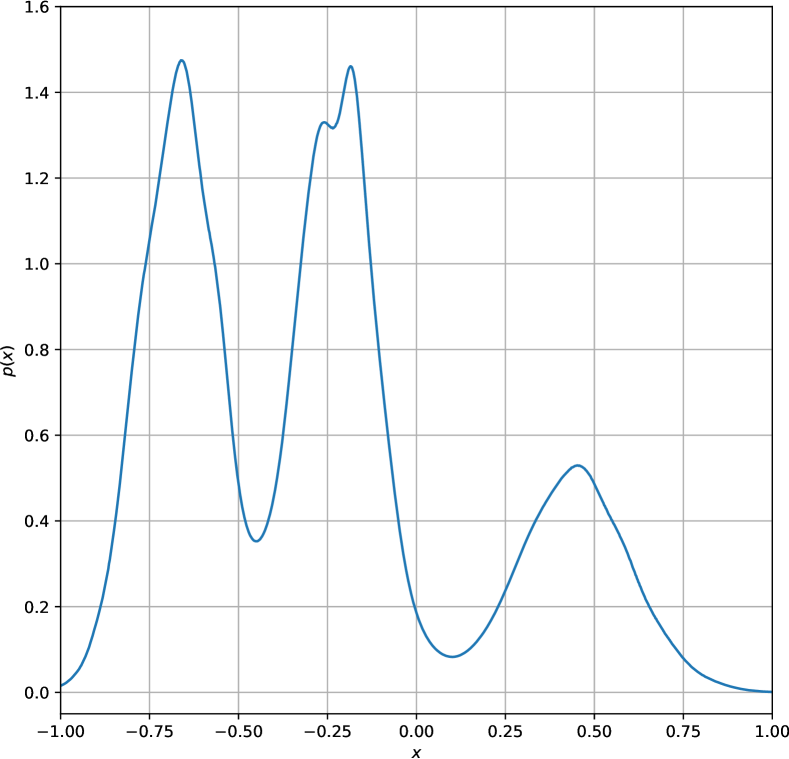
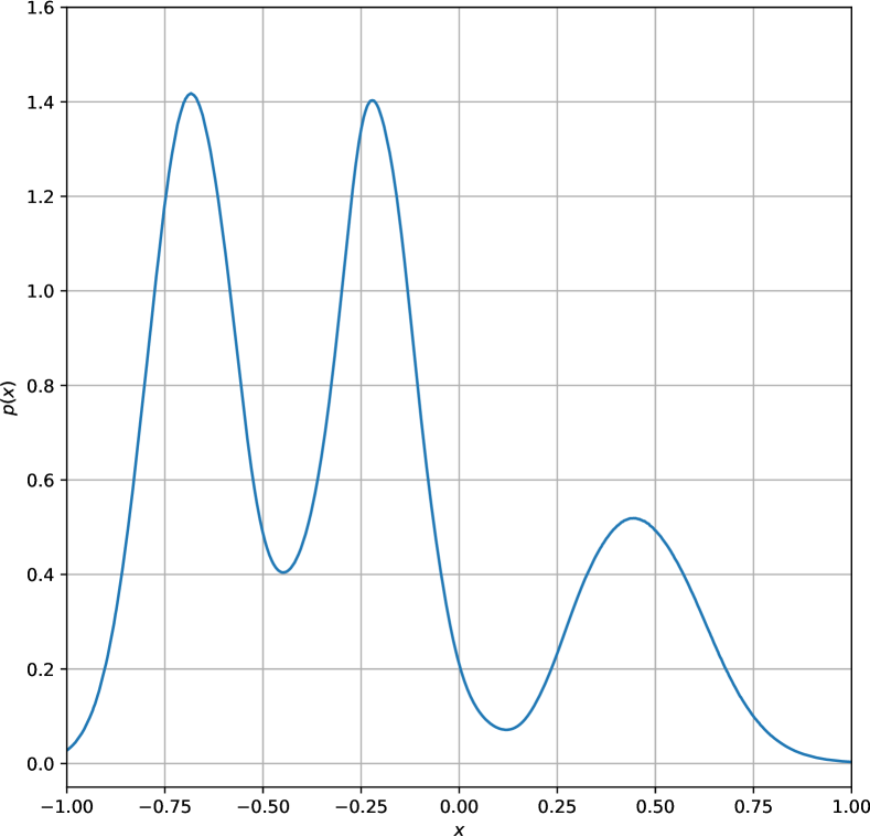
We firstly show that for the ScoreODE of VP type, even on the simple 1-D mixture-of-Gaussians, the model density trained by the first-order DSM is not good enough and can be improved by the third-order DSM, as shown in Fig. 5.
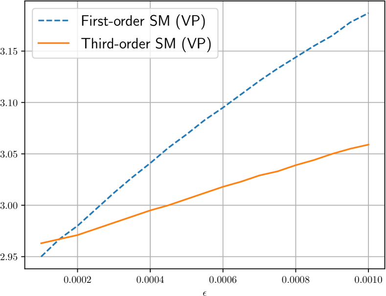
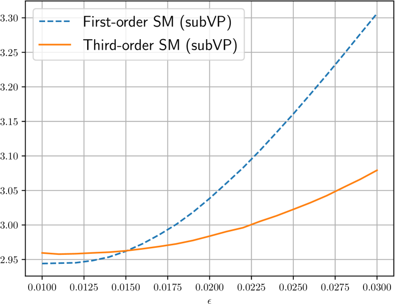
We then train ScoreODE of VP and subVP types on the CIFAR-10 dataset. We use the pretrained checkpoint by first-order DSM in (Song et al., 2021) (the checkpoint of “Baseline+LW+IS”), and further train 100k iterations. We use the same experiment settings as the VE experiments. We vary the start evaluation time and evaluate the model likelihood at each , as shown in Fig. 6. For the ScoreODE trained by the first-order DSM, the model likelihood is poor when is slightly large. Note that Song et al. (2020b, 2021) uses for sampling of VP type, and the corresponding likelihood is poor. Moreover, our proposed method can improve the likelihood for larger than a certain value (e.g. our method can improve the likelihood for the VP type with ). However, for very small , our method cannot improve the likelihood for VP and subVP. We suspect that it is because of the “unbounded score” problem (Dockhorn et al., 2021). The first-order score function suffers numerical issues for near and the first-order SM error is so large that it cannot provide useful information for the higher-order SM.
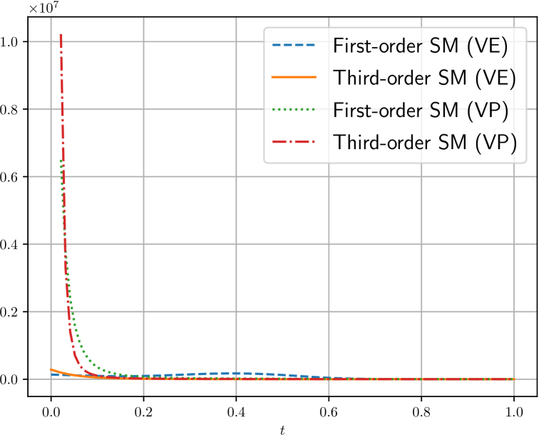
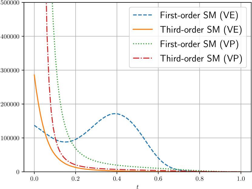
As the data score function is unknown for CIFAR-10 experiments, we cannot evaluate . To show the effectiveness of our method, we evaluate the difference between and in the . Denote
| (208) |
we take time steps between and to evaluate , where the ODE score function is computed by the method in Appendix. D, and the expectation w.r.t. are computed by the Monte-Carlo method, namely we use the test dataset for and then sample from . We evaluate the for the first-order DSM training (baseline) and the third-order DSM training for both the VP and VE types, as shown in Fig. 7. We can find that our proposed high-order DSM method can reduce for ScoreODEs for most . As is an estimation of the true data score function , the results indicates that our proposed method can reduce of ScoreODEs and then further reduce . Also, we can find that the “unbounded score” problem of VE is much milder than that of VP, which can explain why our method can greatly improve the likelihood of VE type even for very small .
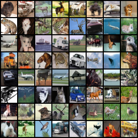
Moreover, we randomly select a batch of generated samples by the PC sampler (Song et al., 2020b) of the same random seed by the VE model of first-order, second-order and third-order DSM training, as shown in Fig. 8. The samples are very close for human eyes, which shows that after our proposed training method, the score model can still be used for the sample methods of SGMs to generate high-quality samples.