ProGNNosis: A Data-driven Model to Predict GNN Computation Time Using Graph Metrics
Abstract
Graph Neural Networks (GNN) show great promise in problems dealing with graph-structured data. One of the unique points of GNNs is their flexibility to adapt to multiple problems, which not only leads to wide applicability, but also poses important challenges when finding the best model or acceleration technique for a particular problem. An example of such challenges resides in the fact that the accuracy or effectiveness of a GNN model or acceleration technique, respectively, generally depends on the structure of the underlying graph. In this paper, in an attempt to address the problem of graph-dependent acceleration, we propose ProGNNosis, a data-driven model that can predict the GNN training time of a given GNN model running over a graph of arbitrary characteristics by inspecting the input graph metrics. Such prediction is made based on a regression that was previously trained offline using a diverse synthetic graph dataset. In practice, our method allows making informed decisions on which design to use for a specific problem. In the paper, the methodology to build ProGNNosis is defined and applied for a specific use case, where it helps to decide which graph representation is better. Our results show that ProGNNosis helps achieve an average speedup of 1.22 over randomly selecting a graph representation in multiple widely used GNN models such as GCN, GIN, GAT, or GraphSAGE.
Index Terms:
Graph neural networks, computation analysis, graph theory, machine learning, characterization, GPUI Introduction
Graph Neural Networks (GNNs) have recently attracted enormous interest in the machine learning community due to their ability to infer from graph-structured data, which other types of neural networks cannot handle efficiently [1]. This has a transformative impact on areas such as recommendation systems [2], natural language processing [3], computer vision [4], particle physics [5], or computer networks [6, 7] as the explosion of recent works can attest.
One of the strengths of GNNs, which make them applicable to a wide variety of problems in multiple domains, is their unique structure and flexibility [8]. Indeed, GNNs can be understood as a family of algorithms allowing to infer features relative to single vertices, edges, or the entire aggregated graphs. However, also due to their wide applicability, not only creating a single GNN model that fits all the scenarios is rendered very difficult, but even the selection of the most accurate GNN model in a specific scenario already becomes a complex and multidimensional problem.
In exchange for such flexibility, GNNs also present unique challenges in their efficient processing due to the variety of GNN variants to support, the inherently alternate execution of dense and very sparse operations, or their dependence on the input graph [9]. As a result, recent works have studied GNNs from a computational workload perspective and attempted to extract the architectural implications of their uniquenesses, aiming to improve their support in CPUs, GPUs, and hardware accelerators [10, 11, 12, 9, 13]. Yet still, solutions that generalize well over all GNN variants and application domains are missing.
Multiple attempts to either maximize the accuracy of a GNN or minimize its processing time have been made. For example, the impact of some design decisions (e.g. the GNN model, the hidden vector size, or the loss function) on the accuracy given a GNN solution has been studied using techniques such as a guided search [14, 15, 16, 17]. A more comprehensive approach is to perform a joint search on both the GNN model and the acceleration technique to navigate the accuracy-processing time tradeoffs of the solution space [18]. However, these works use search methods and try different combinations to then keep the most performant ones. This approach has the problem of spending the time to try different strategies in an ad hoc manner. Another rather new approach is to use a synthetic dataset to see the relationship between the parameters of the graph generator and the accuracy of the different GNN models [19], this allows to explore the relationship between a limited set of characteristics of the graph with the accuracy of the different models and can be used as a benchmarking dataset.
For the analysis of the computation time of GNNs, works are generally infrequent and cover a small design space. One example is the study made in [10], where the impact of the input and output feature vector size is studied for a small selection of GNNs models and datasets. In [20], the authors model the performance and resource efficiency of two hardware accelerators for GNN as functions of several hardware parameters and GNN models but neglecting the irregular connectivity of real graphs. A more comprehensive analysis of the most popular frameworks and GNN models is done in [21], which uses the Open Graph Benchmark (OGB) [22] dataset to make a comparison among GNN acceleration techniques.
Although the OGB suite used in multiple GNN comparison works contains a representative selection of datasets for real-world problems, the span of the suite is limited with most graphs having similar structural characteristics and connectivity, hence failing to cover all possible future application domains. This is an issue due to the dependence of GNNs on the input graph: the accuracy and computation time of a GNN, both in training and inference, generally depends on the aggregation of the features from each node to its neighbors, which is generally extremely sparse and irregular process. In essence, works largely ignore the characteristics of the input graph as they often consider sparsity as the only aspect affecting performance [23, 24], and only evaluate their work on OGB or a smaller selection of graphs.
This paper aims to address these issues by proposing ProGNNosis (Fig. 1), a framework to build data-driven models able to predict the computation time of a specific GNN model executed over a given computation platform, but for a graph of arbitrary characteristics. When repeated over multiple models or computing platforms, possibly with the help of prototyping tools [25], ProGNNosis allows assessing which GNN design will perform better for any type of input graph, without having to perform a search as in prior approaches.
To these ends, ProGNNosis generates a comprehensive and balanced synthetic graph dataset and makes an offline analysis of the impact of the different graph metrics (such as degree distribution and clustering coefficient) on the GNN execution time. Building on this analysis, we demonstrate that a model can be generated that predicts the execution time of the GNN with high accuracy. Then, we establish a simple but representative use case (i.e. the graph representation in memory) and show that we can use ProGNNosis to make informed design decisions about GNN acceleration for any type of graph, achieving a mean speedup of 1.24 for the training set and 1.07 for the testing set with respect to making a random choice in a GCN. We finally repeat the experiment with different GNN models (GIN, GAT, GraphSAGE) to show that the proposed methodology is potentially generalizable, obtaining a mean speedup of 1.26 for the training set and 1.18 for the testing set.
The remainder of the paper is organized as follows. The notation and other preliminary considerations are described in Section II. Our main contribution, a methodology for the data-driven modeling of the execution time of GNNs, is presented in Section III. The methodology is then illustrated for different use cases in Section IV. Finally, the paper is concluded in Section V.

II Preliminaries
A graph is an ordered pair , where is a set of vertices (or nodes) and a set of edges that are connections between pairs of nodes. Stemming from this definition, next we describe the graph metrics, GNN models, and regression and classification considerations used in this work.
II-A Graph Metrics
Graphs are complex structures that can be measured from multiple angles. Depending on the objective of the measurement, different characteristics of the graph can take a central role or have no impact at all. Also, some characterization metrics are correlated and others are not. Another important aspect is the time it takes to calculate the metrics: some metrics can be assessed via a quick inspection of the graph, and others need a great number of calculations, which in some cases can be reduced by obtaining approximate estimates.
In this study, we will use undirected, unweighted, and connected graphs for simplicity. The definitions given in this section will only consider this kind of graph, but the results of the study can be generalized to other kinds of graphs.
Degree: The degree of a node is the number of vertices incident to that node or, in other words, the number of connections a node has. Hence, the degree of a node is generally given by the size of its neighborhood,
| (1) |
where the neighborhood of a node can be defined as Then, the degree distribution can be defined as the fraction of nodes with a given degree. Different characterizations can be extracted from the degree distribution, but some of the most useful ones are the maximum degree, the minimum degree, and the mean degree of a graph. The calculation of the degree distribution can be done in linear order concerning the number of edges in most of the graph representations.
Density: The density of a graph is the ratio between the edges that are present in the graph and the maximum amount of edges that the graph may have, given its number of nodes. Hence, the density of an undirected graph can be defined as:
| (2) |
The density can be calculated in linear order in most of the graph representations, and most of the time the number of nodes and edges is already calculated and stored with the graph.
Clustering coefficient The clustering coefficient of a node can be defined as:
| (3) |
This indicates how close is the neighborhood of that node to generating a complete subgraph (or clique). The mean clustering coefficient is, as its name indicates, the mean of the clustering coefficient of all the nodes in a graph. The computational complexity of calculating the clustering coefficient is . Because of this, we use an approximation to calculate the clustering coefficient that is based on using trials instead of using all the nodes to calculate the coefficient, based on the ideas proposed in [26].
II-B Regression and Classification
In this work, we use regression and/or classification to extract the relationship between the computation time of a GNN model and the characteristics of an input graph, defined by some of the metrics described above.
On the one hand, regression is the statistical process used to find the relationship between a dependent variable and one or more independent variables (or features). The linear regression finds a linear combination of the independent variables that reduce the sum of squared differences with the dependent variable. To measure the performance of regression we will use three metrics:
-
•
The coefficient of determination () is the sum of squared residuals and is 1 if all predictions are correct (best case), is 0 for the baseline model (using always the mean as prediction), and maybe negative if the prediction is worst than the baseline model.
-
•
The mean squared error (MSE) is the mean of the square of the differences between the predicted and the real values. It is 0 if all predictions are correct and its value increases with the errors. Since it grows with the square of the error, it is a good indicator of outliers.
-
•
The mean absolute percentage error (MAPE) is the sum of the errors divided by the real value. MAPE is good to find if the error does grow disproportionate to the real value.
On the other hand, classification is also a statistical process, but in this case, the dependent variable is discrete and each value it can take is called a class. One popular option for classification is the use of Support Vector Machine (SVM), which defines a hyperplane that separates the data into categories. This hyperplane is such that it maximizes the margin between the clases. To measure the performance of classification we will use the accuracy, which is simply the number of correctly classified samples divided by the total number of samples.
II-C GNN Fundamentals
Although GNNs are a wide family of algorithms, in this work we focus on the problem of node classification. The main idea is to use semi-supervised learning, where only some nodes are labeled with their class and the GNN should be able to generalize the labels to the rest of the nodes.
To do so, each node has a vector of input features . With this input vector, the GNN does a series of transformations to obtain , the output vector. In multiclass node classification, the output vector is composed of one slot for each class, the highest number the one corresponding to the class assigned to the node. Each node goes through a series of intermediate states . The final state is , being the number of layers of the GNN.
In general, the -th layer of a GNN can formally be described as:
| (4) |
where is the hidden layer of node on generation , is the aggregate function, whereas is the update function that combines the aggregated result with the previous state of the node.
The training of the model is done through backpropagation to minimize a loss function. In each epoch, the weights update function and, in some models, the aggregate function, are updated after the model is used to predict the labels of the labeled nodes. See [9] for more details on the computations of the training process.
II-D Sample GNN Models
We will now present some of the most popular GNN models, which we employ in this work to evaluate the generalization potential of ProGNNosis. The implementation used in this study for all the models is based on Pytorch Geometric (PyG) [27], which is one of the most used frameworks.
Graph Convolutional Network (GCN): GCN is based on convolutional neural networks, but applied to graphs [28]. It uses a local approximation of the eigenvalues of the adjacency matrix to compute a convolution in the non-euclidean space defined by the graph. The GCN step for a node can be defined as
| (5) |
where are the trainable weights and is a function that introduces a non-linearity, e.g. ReLu. Note that the aggregated features are normalized to the degree of the connected vertices, e.g. .
Graph Isomorphism Network (GIN): GIN is a simple model built to demonstrate that even simple models may be powerful on GNN [29], and aims to classify graphs based on their similarity. The GIN step can be defined as
| (6) |
where is a multi-layer perceptron, and is a parameter of the model that indicates the importance of the nodes own value to the ones of its neighborhood.
Graph Attention Networks (GAT): GAT is based on the concept of attention, where the edges have a learnable weight that changes over the generations depending on the feature vectors of the nodes [30]. The GAT step can be defined as
| (7) |
where is the attention coeficient for nodes and . The attention coefficient can be calculated as
| (8) |
where is the attention function, softmax is the normalization between neighbors, and are the trainable weights.
GraphSAGE (SAGE): GraphSAGE (SAmple and aggreGatE) owes its name to the fact that it samples the neighbors of a node for the aggregation stage [31]. SAGE can be used with different aggregations, we will present here the one we used that is the sum aggregation, which take the form:
| (9) |
where and are the trainable weights.
III ProGNNosis: Approach and Evaluation Methodology
The proposed framework, called ProGNNosis, is able to predict how long will it take for a given GNN to process a certain GNN model in a given computing platform, considering a graph of arbitrary characteristics. With ProGNNosis, we propose to make informed decisions on GNN acceleration or GNN design towards minimizing the training time per generation.
To achieve this objective, we consider a series of steps that are represented in Figure 1:
-
1.
The first step consists in creating a synthetic dataset containing a broad set of graphs of different characteristics. This dataset will help us understand the relationship between different graphs and the training time of a GNN.
-
2.
Using the dataset, we measure the training time for each of the designs that we want to compare for each of the graphs of the dataset.
-
3.
In parallel, we calculate a set of characterization metrics over the graphs of the dataset.
-
4.
Once we have the data, an analysis can be made to understand the correlations between the metrics and the training time of the different models. In particular, a regression model can be built for each of the designs.
-
5.
Finally, the results of the different designs can be compared to classify the graphs into groups that indicate which design performed better. The classification results then are used to corroborate that processing time can be saved by applying this methodology.
Each step of the process can be verified against a testing set, which contains real-world graphs, to see if (i) the synthetic dataset covers the full extent of the testing dataset, (ii) the regression extrapolates to them, and (iii) the classification works correctly with them. The testing set was created using the SparseMatrix collection [32] and a subset of the OGB benchmarks. Graphs were selected to represent the widest selection of domain and graph characteristics.
The resulting set of models can then be used to optimize the processing of other graphs by predicting the processing time of each design using the pre-trained models and using the one that was predicted to perform better.
III-A Synthetic Graph Dataset Generation
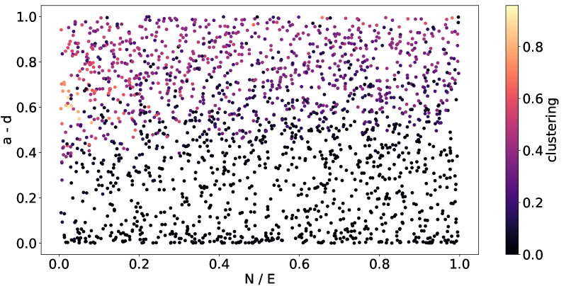
One of the most important aspects of the proposed approach is the creation of a synthetic dataset with diverse characteristics. To create this synthetic dataset, we started by creating a dataset using a naive approach. Then, an optimization problem was stated using this dataset to find a less biased dataset.
To generate the synthetic graphs, the popular RMAT graph generator was used [33]. We selected this tool because it can generate graphs with a wide variety of metrics that can be controlled through its parameters, and also because it is quite performant allowing us to generate large datasets in a short time.
The RMAT generator uses six parameters. The first two parameters are the number of nodes and the number of edges . Then, we have a vector of symmetric parameters that define the fitness distribution for the edge attachment. The vector is a probability vector, and as such the sum of its elements must be 1. The RMAT generator works by dividing the adjacency matrix into four groups recursively and assigning the probability of an edge falling in each of the groups following the vector.
As already stated in the introduction, one aspect that we found to be especially important in the synthetic dataset used as the training set is that graphs with different characteristics are represented. This means that the dataset should have a wide range and balanced representation of values on the different characterization metrics, hence avoiding selection bias (i.e. bias towards a certain combination of metrics). However, we found that datasets generated in a naive way using RMAT had a selection bias towards graphs with low clustering coefficient, among other characteristics, as can be seen in Figure 2.
To overcome this bias, we propose a method where an optimization problem is defined to find an RMAT parameter distribution that generates a less biased dataset [34]. Also, a tool to train and generate the dataset was developed, called Graphlaxy, which was used in this work to generate the synthetic training set. Graphlaxy is open source and available at https://github.com/BNN-UPC/graphlaxy.
III-B Use Case Description
The scenario that we use to demonstrate the use and results of this method consists of comparing two designs that do not affect the GNN accuracy but that do affect the training time. The designs consist of two different ways of processing the GNN, based on two graph representations: SPARSE and EDGE_LIST. The SPARSE representation uses sparse matrix multiplication to compute the aggregation function, whereas the EDGE_LIST representation uses gather and scatter CUDA instructions to compute the aggregation function.
The experiment was repeated for the four different GNN models, described in Section II-C, to show how the results vary depending on the model. To do a fair comparison, all graphs (training and testing set) were populated with a randomly generated set of features and a random class. The feature vectors are assumed of size 32, the hidden layer of size 32, the number of layers is 3 and the number of classes is 2.
All the experiments are run using the same software, the framework (PyG) with CUDA version 10.1 and torch version 1.10.2; as well as the same hardware, a machine with CPU Intel(R) Core(TM) i7-2600 CPU @ 3.40GHz, GPU GeForce GTX 980 Ti and 15 GB of RAM. To reason about the results obtained, executions were profiled using NVIDIA Nsight.
IV Performance Evaluation
In this section, we go through the different steps of the methodology showing the results obtained for the training and testing sets and a short discussion about the intuition behind those results.
IV-A Dataset Generation
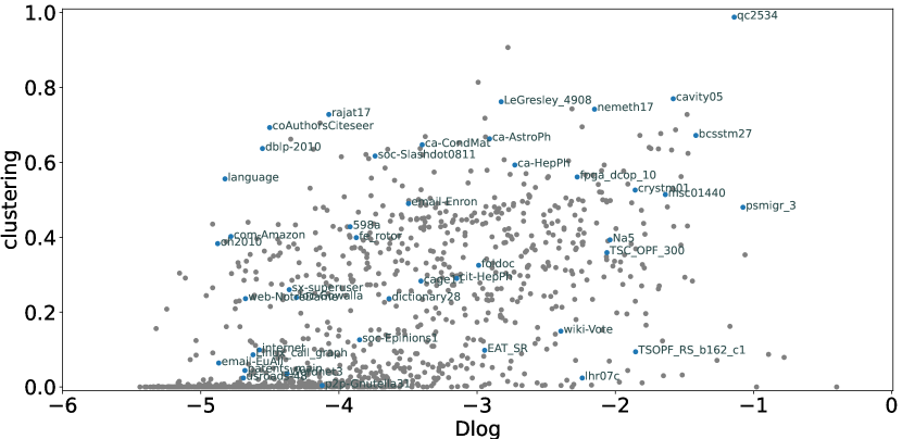
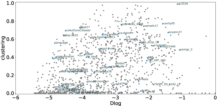
Using the method described in Section III-A, we were able to generate a dataset that represents most of the real graphs used as validation. It can be seen in Figure 3 that, in the naive dataset created with RMAT only, most of the graphs have low clustering coefficients and that some of the real graphs from the validation set have high clustering coefficients, rendering these graphs underrepresented. We can also see that the final dataset generated with Graphlaxy [34] solves this problem and that most graphs from the validation set fall inside the limits of the point cloud corresponding to the graphs in this dataset. The dataset is composed of graphs with edges ranging from one thousand to one million. The number of nodes and the rest of the parameters of RMAT are controlled by a distribution resulting from the optimization problem. Such a broad and balanced dataset will allow us to train a regression that takes into account the relationship between the different variables considered.
IV-B Analysis
Once we have an unbiased dataset, an analysis of the impact of the graph metrics on the computation time can be made. Since the SPARSE representation of the graph is based on sparse matrix multiplication, we pulled some ideas on which are the most impactful metrics in studies on matrix multiplication [35, 36]. In this work, the most impactful metric was the number of non-zero elements, which is translated to graphs as the number of edges. Additionally, through the experiments, we found that the most relevant metrics were the number of nodes, the number of edges, the maximum degree, and the clustering of the graph.
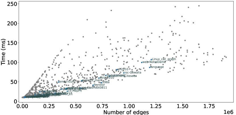
In Figure 4, we can see how the number of edges impacts the computation time of the training set and the validation set. We can see also that there is no linearity when the graphs are small. Also, we see that the variation increases the more edges the graph has, indicating that other metrics could explain that variation. A similar figure can be plotted for all the analyzed configurations, resulting in a similar shape. The impact of these metrics on each of the models and graph representations varies, effectively generating a breakpoint between when each of the designs is preferred, as we see later.
The impact of the number of nodes and number of edges can be explained because they indicate the number of operations on the aggregation, though their influence is different for SPARSE and EDGE_LIST representations. The impact of the maximum degree lies in the fact that highly connected nodes become a bottleneck where all computations of the aggregation on the neighbors must be completed before the calculation of the update. Also, the clustering may be an indicator of the complex dependency between the calculations of the nodes. The non-linearity shown at the left of the graph may be explained by the fact that small graphs use a small portion of the GPU memory and pipeline, and thus slightly bigger graphs use more GPU resources over the same amount of time instead of the same amount of resources during more time. This non-linearity will vary with the hardware used.
IV-C Regression
Configuration Training Testing Model Repr. R^2 MSE MAPE R^2 MSE MAPE GCN Sparse 0.99 3 0.03 0.98 11 0.04 Edge List 0.98 37 0.06 0.97 21 0.09 GIN Sparse 0.99 2 0.04 0.99 1 0.05 Edge List 0.97 68 0.06 0.98 19 0.09 GAT Sparse 0.99 3 0.02 0.99 18 0.03 Edge List 0.99 57 0.04 0.97 50 0.07 SAGE Sparse 0.99 2 0.06 0.99 1 0.07 Edge List 0.97 72 0.08 0.97 20 0.11
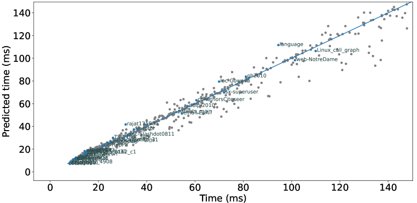
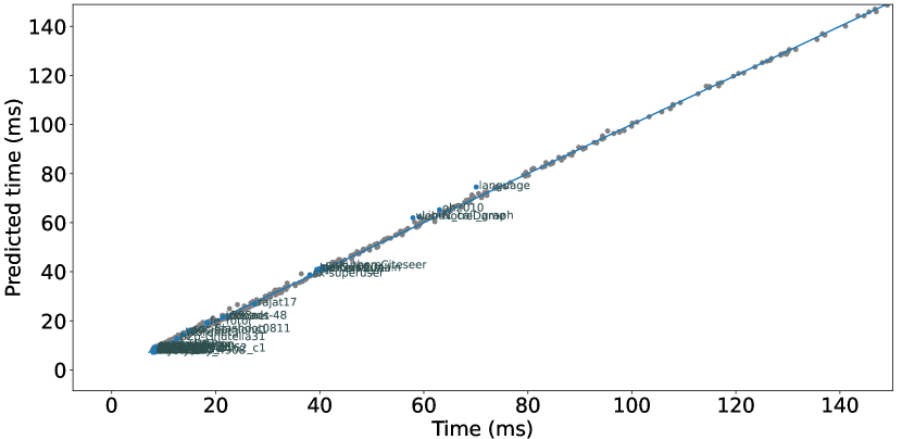
Based on the analysis we made, we built a model using the metrics (number of nodes, number of edges and maximum degree, and the mean degree) able to predict the training time of the different designs with high accuracy (mean of 0.98 in both training and testing set). The model used is a mix of linear regression with ridge normalization and SVM regression with radial basis function kernel (RBF). The SVM is used to predict the residuals of the linear regression to account for the non-linearity. This compound approach was taken because the SVM by itself is unable to generalize to bigger graphs, and the linear regression is unable to fit the non-linear parts of the data.
Table I shows that the results for SPARSE graph representation are in general better than the ones with EDGE_LIST. We see that the MSE is the value that increases more on the validation set for EDGE_LIST indicating that some values have higher errors. In general, we can conclude that the models work well for both representations, though slightly better for SPARSE representation. This can be explained in Figure 5, where we see that the EDGE_LIST representation has a higher variation for the same set of metrics, maybe indicating that one more metric could be used, or because of the implications of the method like the order in which the nodes are processed may impact the performance.
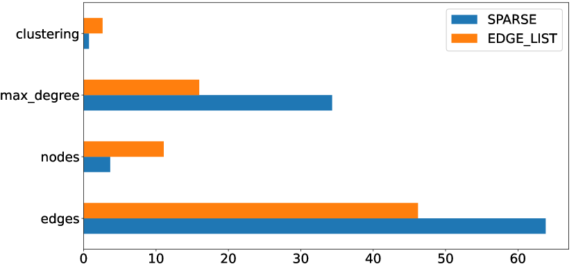
To corroborate what we have observed in the analysis, Figure 6 shows the impact factor, defined as the standard deviation of the variable times the coefficient of the linear regression for each metric. We can see that the number of edges is the more impactful metric, followed by the maximum degree and that the impact of the metric varies from one representation to the other.
IV-D Classification
| Model | training | testing | ||
|---|---|---|---|---|
| accuracy | speedup | accuracy | speedup | |
| GCN | 0.96 | 1.24 | 0.90 | 1.07 |
| GIN | 0.93 | 1.30 | 0.95 | 1.26 |
| GAT | 0.97 | 1.16 | 0.90 | 1.05 |
| SAGE | 0.95 | 1.35 | 0.98 | 1.35 |
Once the regression models are built for each design, the results of the models can be used to classify the graphs by which design will perform better.
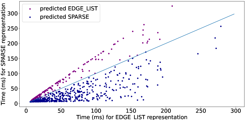
From Table II, we can obtain the accuracy of the classification between graphs that will work better with the SPARSE representations and the ones that will work better with the EDGE_LIST representations. These results are good all over 0.9. From Figure 7, we can see that the graphs that are not being correctly classified are close to the diagonal, meaning that the time for both graph representations is similar. Therefore, classifying them wrongly may have a low impact on the GNN acceleration results.
IV-E Use Case Summary
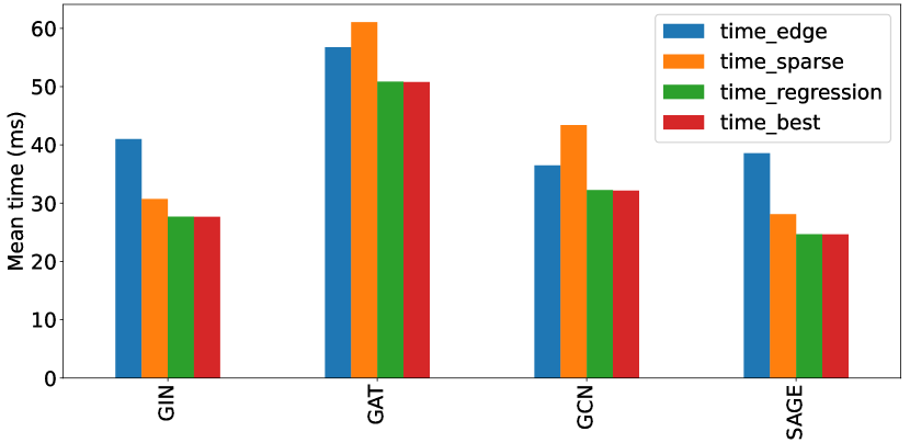
Using the designed method, we demonstrate through Figure 8 that GNN computation can be accelerated through informed decisions. By using ProGNNosis, we can achieve a speedup close to the one we would obtain by always selecting the best option between the two designs. A summary of the obtained speedups is also shown in Table II. Models such as GAT or SAGE showed potential speedups over 1.30. We have also seen that when sweeping other variables out of the scope of this study, such as the number of input features, the tradeoffs vary but, still, ProGNNosis allows to identify the best representation strategy. However, the results are not shown in the paper for the sake of brevity.
V Conclusion
In this study, we have analyzes the impact of different graph metrics on the training time of different GNN models and different graph representations. With these results, we were able to build a model that can predict the training time of different GNN designs. Furthermore, we demonstrated that this method can be used to select the best design in terms of training time for a given GNN model and a graph of arbitrary characteristics. In the presented scenario, we are only comparing the processing time assuming two graph representation alternatives and, even so, we achieved significant speedups of over 1.20 on average and exceeding 1.30 in specific models. However, with a wider design space, the speedups could be increased. In future work, we intend to include the feature vector size and other variables as part of the regression models. Further, the method can be generalized not only to multiple GNN models, as we have seen in this paper, but also to other design variables such as the internal dataflow of a hardware accelerator [12].
It is important to notice that the speedups obtained do not take into consideration the time taken to calculate the metrics, the regression, or the time to transform the graph from one representation to another. Yet still, such pre-processing steps only need to be performed once for each graph and may be done offline depending on the scenario. Also, a tradeoff may be optimized between the approximation used for calculating the metric and the accuracy of the regression. These are left as future work.
References
- [1] Z. Wu, S. Pan, F. Chen, G. Long, C. Zhang, and S. Y. Philip, “A comprehensive survey on graph neural networks,” IEEE Transactions on Neural Networks and Learning Systems, vol. 32, no. 1, pp. 4–24, 2020.
- [2] S. Wu, F. Sun, W. Zhang, X. Xie, and B. Cui, “Graph neural networks in recommender systems: A survey,” ACM Computing Surveys (CSUR), 2022.
- [3] T. Young, D. Hazarika, S. Poria, and E. Cambria, “Recent trends in deep learning based natural language processing,” IEEE Computational Intelligence Magazine, vol. 13, no. 3, pp. 55–75, 2018.
- [4] W. Shi and R. Rajkumar, “Point-GNN: Graph neural network for 3D object detection in a point cloud,” in Proceedings of the IEEE/CVF conference on computer vision and pattern recognition, 2020, pp. 1711–1719.
- [5] X. Ju, S. Farrell, P. Calafiura, D. Murnane, Prabhat, L. Gray et al., “Graph neural networks for particle reconstruction in high energy physics detectors,” in Second Workshop on Machine Learning and the Physical Sciences (NeurIPS 2019), 2019.
- [6] K. Rusek, J. Suárez-Varela, P. Almasan, P. Barlet-Ros, and A. Cabellos-Aparicio, “RouteNet: Leveraging Graph Neural Networks for network modeling and optimization in SDN,” IEEE Journal on Selected Areas in Communications, vol. 38, no. 10, pp. 2260–2270, 2020.
- [7] M. Ferriol-Galmés, K. Rusek, J. Suárez-Varela, S. Xiao, X. Cheng, P. Barlet-Ros, and A. Cabellos-Aparicio, “RouteNet-Erlang: A graph neural network for network performance evaluation,” in IEEE International Conference on Computer Communications, 2022.
- [8] J. Zhou, G. Cui, S. Hu, Z. Zhang, C. Yang, Z. Liu, L. Wang, C. Li, and M. Sun, “Graph neural networks: A review of methods and applications,” AI Open, vol. 1, pp. 57–81, 2020.
- [9] S. Abadal, A. Jain, R. Guirado, J. López-Alonso, and E. Alarcón, “Computing graph neural networks: A survey from algorithms to accelerators,” ACM Computing Surveys (CSUR), vol. 54, no. 9, pp. 1–38, 2021.
- [10] M. Yan, Z. Chen, L. Deng, X. Ye, Z. Zhang, D. Fan, and Y. Xie, “Characterizing and understanding GCNs on GPU,” IEEE Computer Architecture Letters, vol. 19, no. 1, pp. 22–25, 2020.
- [11] Z. Zhang, J. Leng, L. Ma, Y. Miao, C. Li, and M. Guo, “Architectural Implications of Graph Neural Networks,” IEEE Computer Architecture Letters, vol. 19, no. 1, pp. 59–62, 2020.
- [12] R. Garg, E. Qin, F. Muñoz-Martínez, R. Guirado, A. Jain, S. Abadal, J. L. Abellán, M. E. Acacio, E. Alarcón, S. Rajamanickam et al., “Understanding the design space of sparse/dense multiphase dataflows for mapping graph neural networks on spatial accelerators,” in 2022 IEEE International Parallel & Distributed Processing Symposium (IPDPS’22). IEEE, 2022.
- [13] X. Liu, M. Yan, L. Deng, G. Li, X. Ye, D. Fan, S. Pan, and Y. Xie, “Survey on graph neural network acceleration: An algorithmic perspective,” arXiv preprint arXiv:2202.04822, 2022.
- [14] K. Zhou, Q. Song, X. Huang, and X. Hu, “Auto-GNN: Neural architecture search of graph neural networks,” arXiv preprint arXiv:1909.03184, 2019.
- [15] K.-H. Lai, D. Zha, K. Zhou, and X. Hu, “Policy-GNN: Aggregation optimization for graph neural networks,” in Proceedings of the 26th ACM SIGKDD International Conference on Knowledge Discovery & Data Mining, 2020, pp. 461–471.
- [16] X. Wang and W. Zhu, “Automated machine learning on graph,” in Proceedings of the 27th ACM SIGKDD Conference on Knowledge Discovery & Data Mining, 2021, pp. 4082–4083.
- [17] J. You, Z. Ying, and J. Leskovec, “Design space for graph neural networks,” Advances in Neural Information Processing Systems, vol. 33, pp. 17 009–17 021, 2020.
- [18] Y. Zhang, H. You, Y. Fu, T. Geng, A. Li, and Y. Lin, “G-CoS: GNN-Accelerator co-search towards both better accuracy and efficiency,” in 2021 IEEE/ACM International Conference On Computer Aided Design (ICCAD). IEEE, 2021, pp. 1–9.
- [19] J. Palowitch, A. Tsitsulin, B. Mayer, and B. Perozzi, “Graphworld: Fake graphs bring real insights for gnns,” arXiv preprint arXiv:2203.00112, 2022.
- [20] R. Guirado, A. Jain, S. Abadal, and E. Alarcón, “Characterizing the communication requirements of GNN accelerators: A model-based approach,” in 2021 IEEE International Symposium on Circuits and Systems (ISCAS). IEEE, 2021.
- [21] J. Wu, J. Sun, H. Sun, and G. Sun, “Performance analysis of graph neural network frameworks,” in 2021 IEEE International Symposium on Performance Analysis of Systems and Software (ISPASS), 2021, pp. 118–127.
- [22] W. Hu, M. Fey, M. Zitnik, Y. Dong, H. Ren, B. Liu, M. Catasta, and J. Leskovec, “Open graph benchmark: Datasets for machine learning on graphs,” arXiv preprint arXiv:2005.00687, 2020.
- [23] C. Tian, L. Ma, Z. Yang, and Y. Dai, “PCGCN: Partition-Centric Processing for Accelerating Graph Convolutional Network,” Proceedings of the IPDPS’20, pp. 936–945, 2020.
- [24] Y. Wang, B. Feng, and Y. Ding, “TC-GNN: accelerating sparse graph neural network computation via dense tensor core on GPUs,” arXiv preprint arXiv:2112.02052, 2021.
- [25] D. Pujol-Perich, J. Suárez-Varela, M. Ferriol, S. Xiao, B. Wu, A. Cabellos-Aparicio, and P. Barlet-Ros, “IGNNITION: bridging the gap between graph neural networks and networking systems,” IEEE Network, vol. 35, no. 6, pp. 171–177, 2021.
- [26] T. Schank and D. Wagner, “Approximating clustering coefficient and transitivity.” Journal of Graph Algorithms and Applications, vol. 9, no. 2, pp. 265–275, 2005.
- [27] M. Fey and J. E. Lenssen, “Fast graph representation learning with pytorch geometric,” arXiv preprint arXiv:1903.02428, 2019.
- [28] T. N. Kipf and M. Welling, “Semi-supervised classification with graph convolutional networks,” arXiv preprint arXiv:1609.02907, 2016.
- [29] K. Xu, W. Hu, J. Leskovec, and S. Jegelka, “How powerful are graph neural networks?” arXiv preprint arXiv:1810.00826, 2018.
- [30] P. Veličković, G. Cucurull, A. Casanova, A. Romero, P. Lio, and Y. Bengio, “Graph attention networks,” arXiv preprint arXiv:1710.10903, 2017.
- [31] W. Hamilton, Z. Ying, and J. Leskovec, “Inductive representation learning on large graphs,” Advances in neural information processing systems, vol. 30, 2017.
- [32] S. P. Kolodziej, M. Aznaveh, M. Bullock, J. David, T. A. Davis, M. Henderson, Y. Hu, and R. Sandstrom, “The suitesparse matrix collection website interface,” Journal of Open Source Software, vol. 4, no. 35, p. 1244, 2019.
- [33] D. Chakrabarti, Y. Zhan, and C. Faloutsos, “R-MAT: A recursive model for graph mining,” in Proceedings of the 2004 SIAM International Conference on Data Mining. SIAM, 2004, pp. 442–446.
- [34] A. Wassington and S. Abadal, “Bias reduction via cooperative bargaining in synthetic graph dataset generation,” arXiv preprint arXiv:2205.13901, 2022.
- [35] D. Castaño-Díez, D. Moser, A. Schoenegger, S. Pruggnaller, and A. S. Frangakis, “Performance evaluation of image processing algorithms on the GPU,” Journal of structural biology, vol. 164, no. 1, pp. 153–160, 2008.
- [36] J.-S. Yeom, J. J. Thiagarajan, A. Bhatele, G. Bronevetsky, and T. Kolev, “Data-driven performance modeling of linear solvers for sparse matrices,” in 2016 7th International Workshop on Performance Modeling, Benchmarking and Simulation of High Performance Computer Systems (PMBS). IEEE, 2016, pp. 32–42.
| Axel Wassington Biography text here. |
| Sergi Abadal Biography text here. |