On the Surprising Behaviour of node2vec
Abstract
Graph embedding techniques are a staple of modern graph learning research. When using embeddings for downstream tasks such as classification, information about their stability and robustness, i.e., their susceptibility to sources of noise, stochastic effects, or specific parameter choices, becomes increasingly important. As one of the most prominent graph embedding schemes, we focus on node2vec and analyse its embedding quality from multiple perspectives. Our findings indicate that embedding quality is unstable with respect to parameter choices, and we propose strategies to remedy this in practice.
1 Introduction
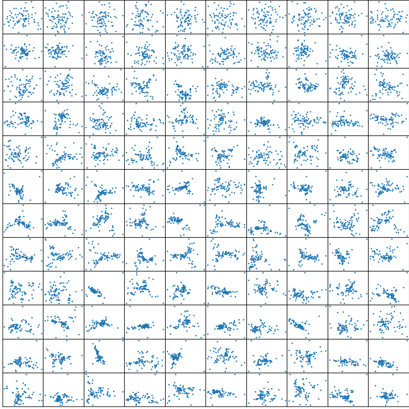
Graph representation learning methods are used in numerous tasks, such as graph classification, that require representing a given data set as elements in a Euclidean space. Many of these methods involve a certain amount of stochasticity. In node2vec Grover & Leskovec (2016), for instance, stochasticity is present at several stages of the algorithms, namely in the random walks themselves and in the random initialization and optimization of the algorithm. This algorithm also depends on a number of parameters, chosen by the user, such as (i) the length of random walks, (ii) the number of random walks, (iii) the dimension of the target vector space, and (iv) the neighbourhood size. Hence, the resulting embeddings can vary considerably. This is illustrated in Figure 1, which depicts low-dimensional projections of different embeddings of the “Les Misérables” character co-occurrence network (Knuth, 1994).
In practice, graph representation learning methods are often used under the assumption that their outputs give a desired result, without formal evidence, and any potential variability in the resulting embeddings is not commonly studied. We stress that this is not a unique characteristic of node2vec, and other methods are also prone to it (Grohe, 2020; Hacker, 2020); however, in the interest of conciseness, our paper focuses only on node2vec. In Hajij et al. (2021), for example, node2vec is applied to a graph to obtain a map . This map is then used to create a filtration of the graph and compute persistent homology (see e.g. Hensel et al. (2021) for a recent survey). In neuroscience, node2vec has been used in several contexts (Rosenthal et al., 2018; Levakov et al., 2021), where the embeddings of connectomes have been used to approximate functional connectomes from the embeddings of the structural ones. However, in none of these applications nor in others is it formally taken into account that the results could greatly depend on the differences in the resulting embeddings. Since in principle, the outputs of the algorithm can be different, even if the parameters are well chosen (for instance with respect to a specific task), it is important to understand the stability of these methods in order to draw coherent conclusions about the data.
Previous research (Goyal & Ferrara, 2018; Hacker, 2020) suggests that, at least within a range of parameters, there is a form of stability at a macroscopic level. The clusters found in the point clouds recover almost exactly the combinatorial type of nodes of the graph or simplices found in the clique complex of the original graph. The stability exhibited at a macroscopic level motivates a more formal study of stability, at a more granular level exploring local structures of the embeddings. Some existing approaches to the question are explained in Section 2. In Section 3, we present our own approach to this question, while Section 4 provides the results of our experiments.
Contributions.
We study the structural stability of node2vec in a more formal framework by evaluating embeddings generated from varying sets of parameters to capture the differences that can be induced by different choices of parameters. We incorporate both “real-world” graph data sets and well-understood random graph models, which will serve as null models. Overall, we find that node2vec embeddings can be unstable even for related parameter sets, prompting additional investigations into the stability and overall veracity of an embedding.
2 Background and Related Work
We provide below a short reminder of the node2vec algorithm; more details can be found in Grover & Leskovec (2016). There are several parameters to be chosen by the user, namely the length of random walks, the number of random walks starting at each node of the graph, the dimension of the embedding space, and the neighbourhood size . In the random walks one can also choose two parameters which govern the random walks by biasing them towards different behaviours. Briefly, node2vec (see the appendix111See https://arxiv.org/abs/2206.08252. for algorithmic details), can be divided into the following main steps
-
1.
Compute a collection of truncated random walks, with biases , all of length , such that there are precisely starting at each node of the graph.
-
2.
Using the random walks as a way to extract a measure of similarity between nodes, compute a representation of the nodes, with the paradigm that nodes that co-occur more often in random walks should be more likely to close by in the Euclidean representation.
- 3.
We want to study the stability of node2vec more formally. As outlined above, there are several sources of randomness in the two algorithms, namely in the random walks themselves, in the initialization and training of the network. One could take the approach of controlling stability at each step of the algorithm in order to gauge the overall stability. The approach in this paper will be to first understand the stability of the outputs without controlling the stability of each intermediate step. However, this question is very broad and complex. In this paper, we propose a preliminary approach to this question by studying empirically the effects of the change of parameters on the embeddings, using various measures to assess the stability of the embedding at the microscopic level.
Related work.
Although no formal theoretical study of stability has been provided yet, several approaches to assess “how good” graph embedding methods are have been explored, see for instance Schumacher et al. (2020); Bonner et al. (2017); Xin et al. (2019) for the study of the stability of various graph representation learning methods. These are all empirical approaches. Providing a theoretical framework for this question has proven to be a difficult task given the many parameters to control, even in the simplest cases. The aforementioned literature presents two approaches to deciding whether graph embeddings are good or not are proposed: an approach based on task evaluation and a more structural or geometric approach. In the task evaluation approach, the embedding method is usually evaluated on the quality of a downstream task, such as graph classification. This is studied for example in Schumacher et al. (2020). The drawback of such a method is that it can be specifically tested only on labelled graphs. At the intersection of the structural and task approach, one finds tasks such as link and topological feature prediction (Bonner et al., 2017; Xin et al., 2019). In the structural or geometric approach, the graph embeddings are evaluated on “how well” the embeddings reflect some aspects of the graph structure. Aspects that can be evaluated include graph reconstruction, comparison of degree distributions between that of the original and reconstructed graphs, and cluster preservation. These are then evaluated using various measures for each aspect (Xin et al., 2019). Each measured aspect takes into account different scales of the graph structure, going from a local scale where the method is evaluated around each node, to a more global scale where the preservation of the community structure is measured. The former was already studied to some extent in Hacker (2020) for -simplex2vec and in Goyal & Ferrara (2018) for node2vec and similar methods. These are more related to the question of stability where the central question is: “for a small variation in the hyperparameters of the algorithm or in the graph structure, is the variation of all criteria described above small as well?” Some drawbacks of the evaluation methods presented in Bonner et al. (2017); Xin et al. (2019) is that they evaluate the embeddings only for a fixed choice of parameters for the embedding algorithms, thus lacking an overview of the overall stability of the methods, omitting the potential effects of the parameters on the embeddings.
3 Methods
We consider node2vec as a method to produce a map , i.e., a map from the set of nodes of a graph to a -dimensional vector space. Hence, can be considered as creating a point cloud from a graph or, equivalently, assigning to each node in the graph a vector . The advantage of this perspective is that our analysis and suggestions apply to a wide variety of embedding schemes, including graph neural networks. Hence, instead of assessing the mapping directly, we assess in terms of its empirical outputs. To gauge the output of node2vec, we analyse its stability and quality. The former term refers to the desirable property that embeddings generated by node2vec should be similar222We provide a more precise notion of this similarity below. to each other across different runs of the algorithm with the same hyperparameters, whereas the latter term refers to the need for prroducing embeddings that are useful in downstream tasks, such as the node classification or general knowledge extraction tasks.
3.1 Stability
Our definition of stability is based on the observation that node2vec, like other embedding algorithms, requires the choice of several parameters. Moreover, due to the way the embeddings are constructed, there is a degree of stochasticity involved—the initialisation of the optimiser, for instance, has an impact on the output. We consider an embedding scheme to be stable if its outputs are “reasonably close” for parameter sets that are “reasonably close.” More formally, assuming that and refer to embeddings of the same graph, obtained from parameter sets and , respectively, we want
| (1) |
In other words, the distance between embeddings and should be proportional to the distance between their parameter sets, for some appropriate choice of distance in each case.333Here, we use a simple distance based on the Hamming metric between parameter sets to obtain a consistent ordering between parameter sets. We leave a more detailed analysis of this equation for future work. We argue that this is a natural desirable property of an algorithm because it implies that all conclusions drawn from a specific embedding change in a predictable way as one chooses different parameters.
To assess the stability of embeddings, we will make use of two measures for comparing point clouds. First, the Hausdorff distance between two point clouds is defined as
| (2) |
with , i.e., the minimum distance from to the point cloud , and vice versa for . The Hausdorff distance is easy to calculate but relies on the relative positions of the point clouds and in . Hence, the distance is sensitive to the position of the two point clouds.
To account for small changes in their relative positions,444A more advanced option would be to register point clouds first in order to be invariant to rotations and translations. We leave this for future work. we will also work with the Wasserstein distance of order 2,
| (3) |
ranging over all bijections between the two point clouds, where we compare embeddings computed from the same graph.
Given point clouds , arising from the same parameter set , we can calculate their inter-group distances via the two metrics defined above. If node2vec is stable for , we expect low variance of such distances. Moreover, following Eq. 1, we permit that the distributions of inter-group distances become markedly different as the respective parameter sets become increasingly different. For instance, increasing the number of random walks from to may result in distributions that are close (in the statistical sense), whereas going from to walks could result in distributions that are dissimilar to each other.
3.2 Quality
The assessment of the quality of an embedding is distinct from its stability. For instance, node2vec could be replaced by a simple map that assigns each graph to the zero vector. Such an embedding would be perfectly stable but its output is virtually useless in practice. In the context of graph learning, embedding quality is often measured in terms of predictive performance for a specific task, e.g., how well the embedding serves to preserve important nodes or communities. Since we want to cover situations in which we evaluate node2vec without a specific ground truth, we need task-independent quality measures.
3.2.1 Link distribution comparison
Inspired by Xin et al. (2019), we first measure the dissimilarity between the link distributions of a graph and a link distribution computed using its embedding. Letting refer to the adjacency matrix of a graph , we first obtain the observed link distribution as . provides the probability of an edge , under the assumption that edges are uniformly distributed. In an embedding of , we do not have access to observed edges. However, we may use a similarity measure between the representations of individual nodes , giving rise to an empirical link distribution Xin et al. (2019) via
| (4) |
with referring to the representations of vertices , respectively. Notice that this distribution requires normalisation to constitute a proper probability distribution. There are numerous choices for realising in practice; following Xin et al. (2019), we pick the standard Euclidean inner product of , i.e., , also known as a linear kernel. Since node2vec incorporates a similar objective—its training involves minimising inner product expressions—this formulation has proven useful to assess the output of embedding algorithms Grohe (2020). This formulation provides us with a suitable quality assessment strategy: taking any measure of statistical distance , we use as an indicator of the quality of an embedding . This has the advantage of being immediately interpretable: lower values indicate a better “fit,” in the sense that the resulting embedding preserves the link distribution of a graph, thus permitting a reconstruction.
To implement , we use the Wasserstein distance; while Xin et al. (2019) suggest using a KL divergence, we prefer the Wasserstein distance because it constitutes a proper metric between probability distributions, satisfying in particular symmetry and the triangle inequality, two properties that are indispensable when comparing different embeddings across parameter sets. One advantageous property of this quality assessment procedure is that it is independent of the dimensionality of the embeddings; we can thus compare the distributions across all parameter sets.
3.2.2 Link reconstruction
As a second measure for assessing the quality of embeddings, we consider the previously-defined similarity scores between nodes, i.e., , to be a score of classifier that aims to predict the existence of an edge. Writing to denote , we consider superlevel sets of the form , for . For each choice of , we treat as the set of all edges predicted by the classifier. Ranging over all possible choices for , we calculate a contingency table containing the number of true positives (TP; edges that are correctly predicted), true negatives (TN; non-edges that are correctly predicted, i.e., edges that are not part of a specific ), false positives (FP), and false negatives (FN), respectively. This permits us to calculate precision–recall values, and we take the area under the precision–recall curve (AUPRC) to be a measure of the quality of an embedding (Fawcett, 2006).
AUROC.
Alternatively, we could use the TP and FP values to calculate a receiver–operating characteristic curve and use its area, known as AUC or AUROC, as a measure (Fawcett, 2006). This is more complicated to interpret in most cases, though, since AUROC assumes a binary classification task in which two classes have roughly similar sizes. However, most real-life graphs are highly-imbalanced: out of all the potential edges, only a fraction of them ever exists; a classifier that never predicts any edges based on an embedding would thus score high in terms of AUROC.
4 Experiments
We run node2vec on several different models of graphs on a grid of parameters, using the co-occurrence network of “Les Misérables” (Knuth, 1994), as well as stochastic block models (SBMs), exhibiting well-defined community structures. To prevent additional stochastic effects, we focus on embedding a single instance of the SBM graphs only (using a fixed random seed for the generation of the graph), as opposed to working with data sets of multiple graphs.555 We performed similar analyses for Erdös-Rényi graphs, but found no substantial differences to the results presented here.
Implementation.
We implemented our analysis in Python, using scikit-learn and pytorch; our code is publicly available under a 3-Clause BSD License.666https://github.com/aidos-lab/node2vec-surprises
Experimental setup.
The first stochastic block model (sbm2) has two blocks of nodes and intra-block probability and inter-block probability . The second stochastic block model (sbm3) has three blocks of nodes with intra-block probabilities and inter-block probability of . For each of these graphs, we run node2vec 10 times for each combination of parameters, to assess the variance of the algorithm. Our training procedure uses “early stopping” based on the loss, and we used the following hyperparameter grid: , , and , . Similar to Grover & Leskovec (2016), we use a fixed number of random walks to limit the complexity of the problem.777We consider our work to be a preliminary study of the stability of node2vec and related methods; future work could tackle even more complex hyperparameter grids. In total, this parameter grid provides us with an in-depth view of the performance of node2vec.
Pre-processing.
To simplify the comparisons of different embeddings from a same feature space , we normalise each point cloud so that its diameter is . This has no consequences for quality assessment, but ensures that point clouds remain comparable for the stability analysis.
4.1 Analysis of “Les Misérables”
Following the original publication Grover & Leskovec (2016), we first analysed the “Les Misérables” character co-occurrence network. Figure 1 depicts different embeddings, obtained by applying Principal Component Analysis (PCA) to the node embeddings generated by node2vec. Each point in such a plot corresponds to a single node of the graph. Already in these low-dimensional plots, a large degree of variability becomes apparent—the resulting point clouds have different appearances, even if we only consider runs with the same parameter set, i.e., all point clouds of a single row of Figure 1; we acknowledge that variations in the appearance of embeddings can also be a consequence of PCA. However, the illustration mimics the general usage of node2vec in a data analysis context, where embedding algorithms are typically used to acquire additional insights or solve data analysis tasks.
Subsequently, we will proceed with direct analyses of the high-dimensional embeddings, excluding additional dimensionality reduction algorithms to ensure that we can assess the stability and quality of node2vec without adding a source of potential noise. Knowing that embeddings of high-dimensional data sets are prone to incorrect interpretations, we now turn towards a more principled analysis of the individual point clouds, according to the measures outlined in Section 3.1 and Section 3.2.
Stability.
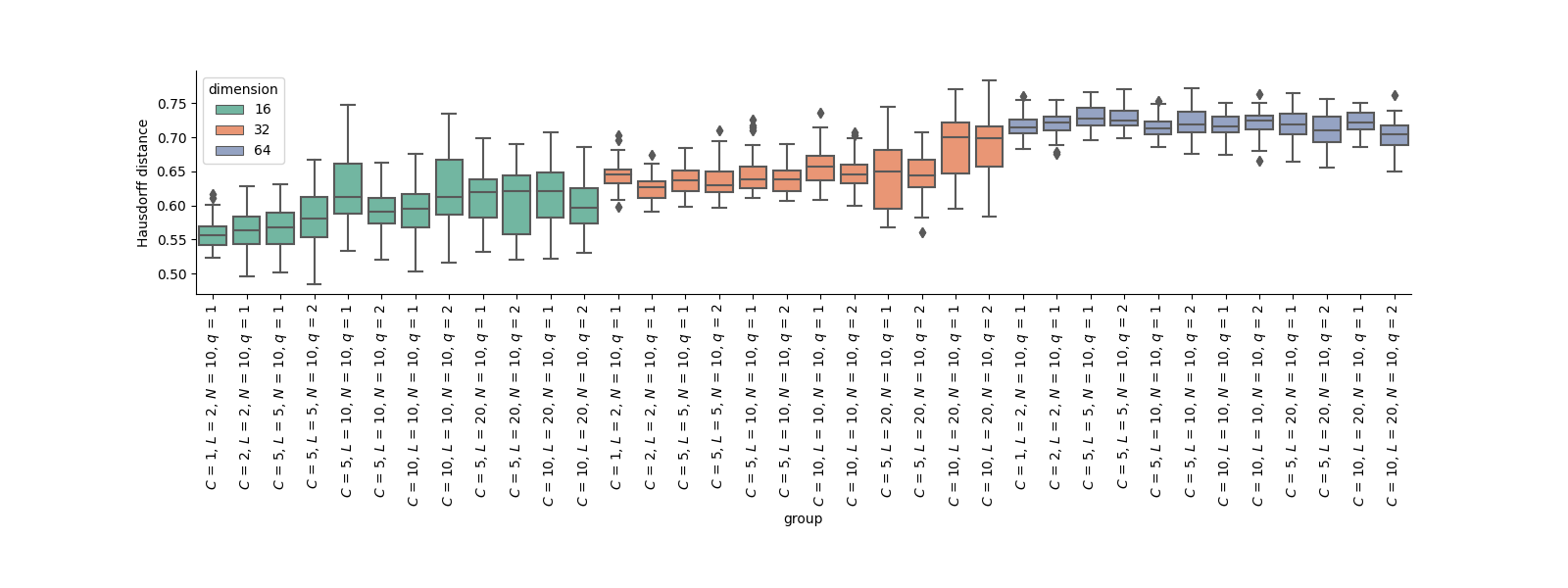
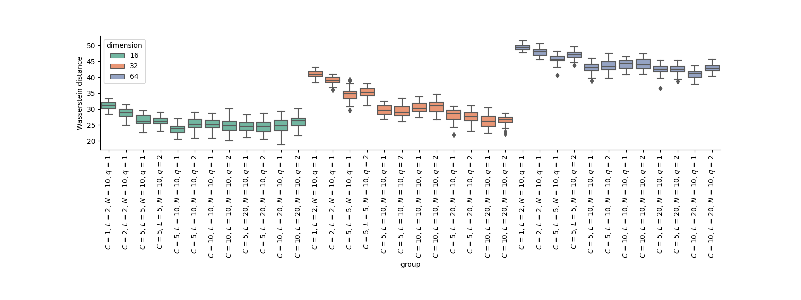
Figure 2 depicts distance distributions for this data set. The Hausdorff distance exhibits a larger variance, even within a set of hyperparameters, i.e., over different repetitions of the same embedding. The Wasserstein distance, by contrast, exhibits smaller variance, hinting at its improved ability to account for some—not all—transformations of the embeddings that are due to stochasticity. Using a Wilcoxon signed-rank test (Wilcoxon, 1945), we find that [] of all pairwise comparisons between hyperparameter groups are found to be statistically significantly different from each other for the Hausdorff [Wasserstein] distance ( with Bonferroni correction). This finding indicates that even if hyperparameter sets differ only by a single value, (i) the resulting distribution of distances between individual embeddings can be substantially different, and (ii) these differences are pronounced enough to be detected by standard tests of statistical significance.
Quality.
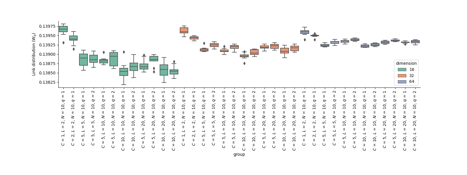
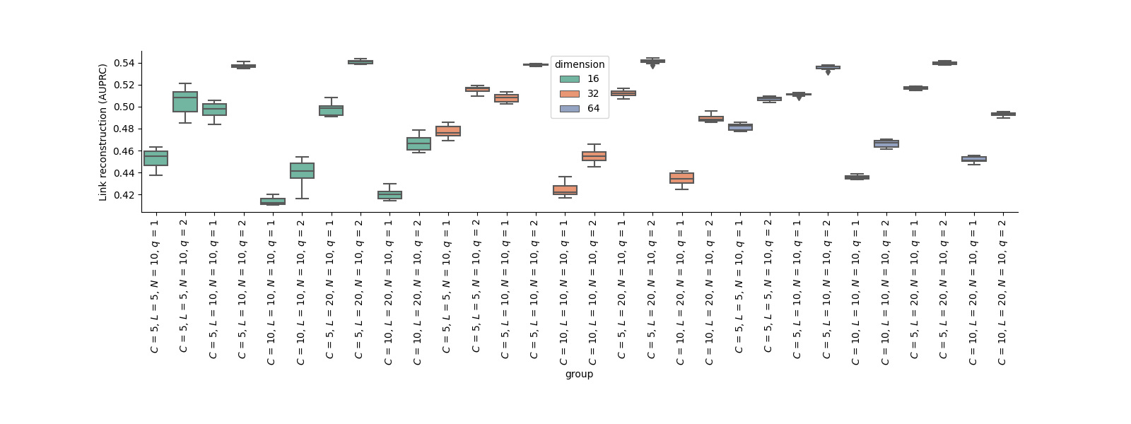
The experiments mentioned above illustrate various ways in which the embeddings appear to be unstable. To form a clearer picture of this problem, we also assessed quality by aiming to reconstruct the edges in the graph. Figure 3 depicts the results. We observe that there is a large degree of variance even for a single parameter set. Somewhat surprisingly, some parameter sets achieve very low AUPRC values, failing to go well beyond random predictions (AUPRC ). The variance for certain choices of parameters—regardless of embedding dimensionality—is still high, indicating that even a careful selection of data-appropriate parameters does not necessarily lead to consistently faithful embeddings.
4.2 Stochastic block models
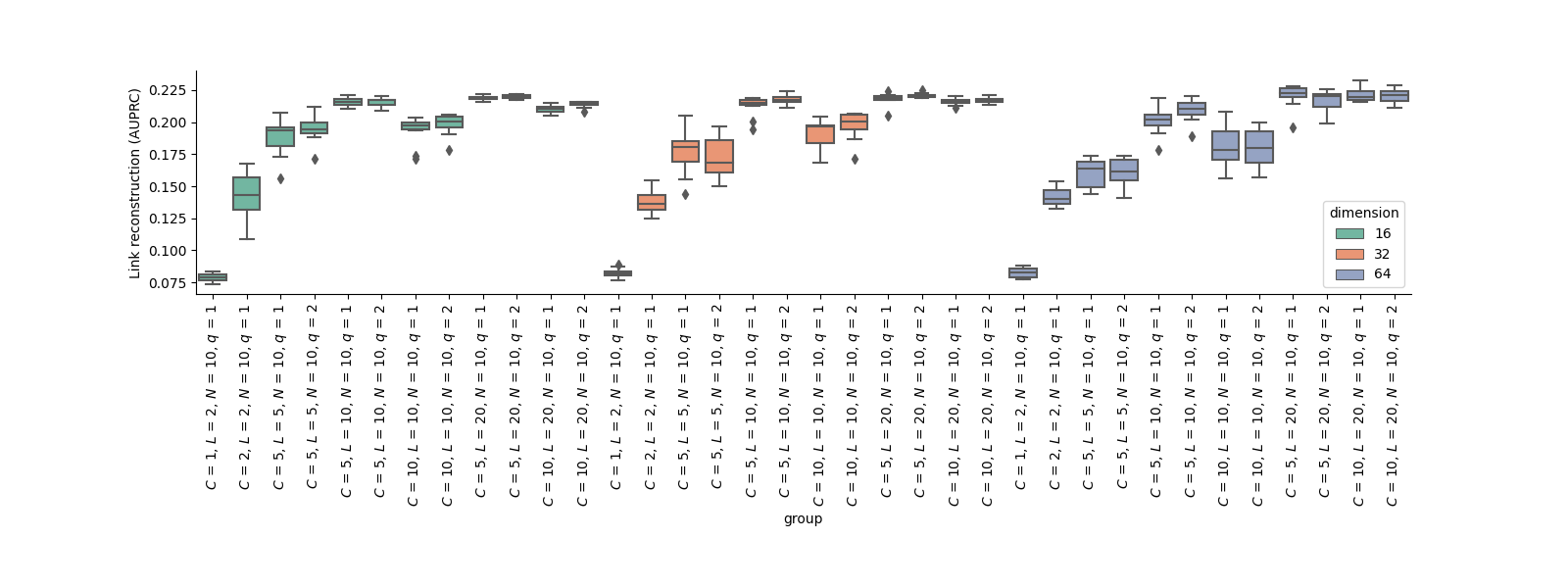
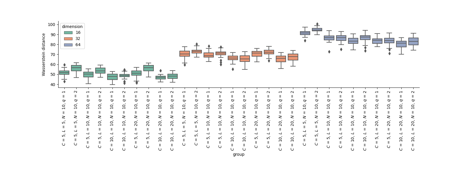
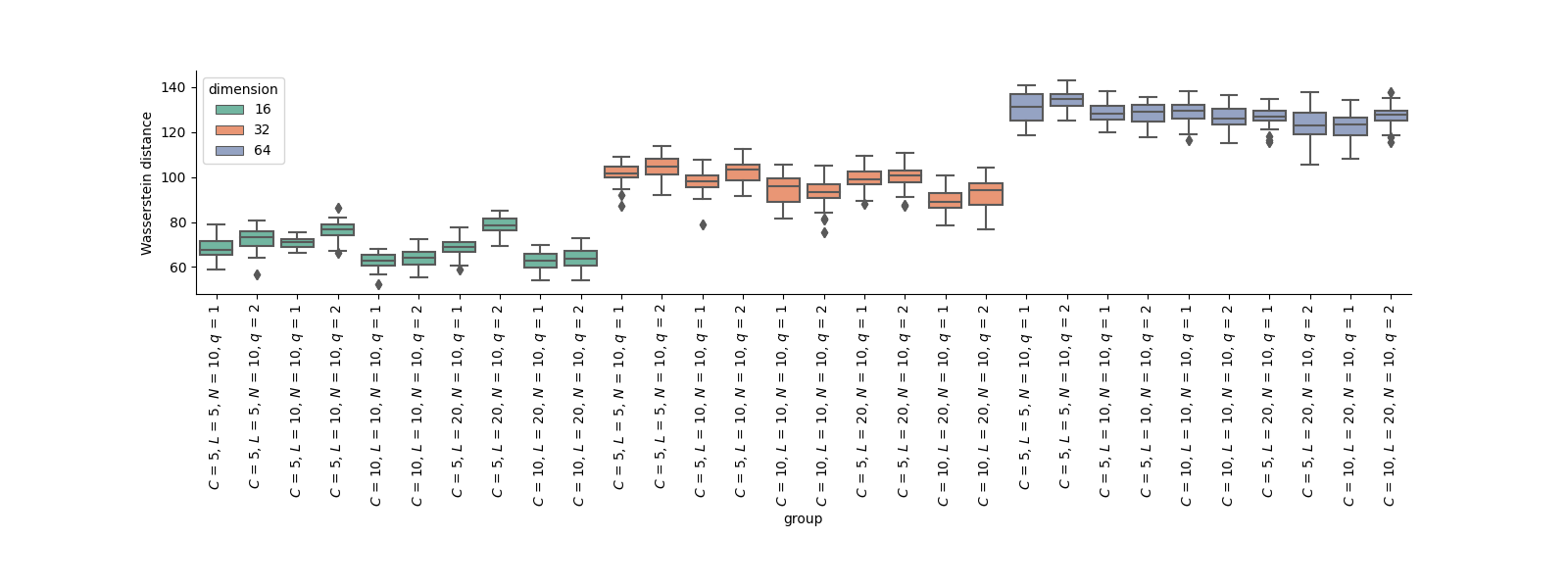
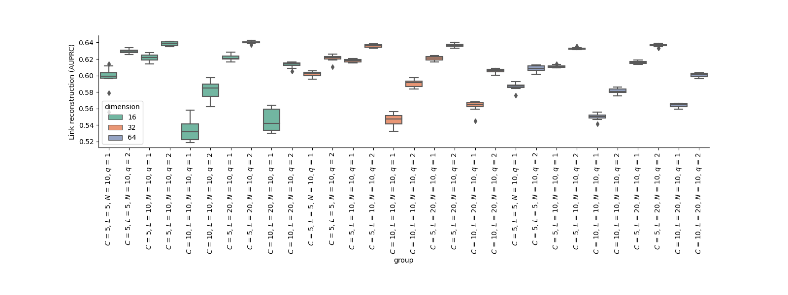
We subject two different graphs arising from a stochastic block model formulation to the analysis described above; sbm2 has two communities, whereas sbm3 has three. Figure 4 shows Wasserstein distance distributions to assess the quality of the embeddings. Similar to the “Les Misérables” graph, of all distributions are statistically significantly different from each other, despite being obtained via highly similar parameter sets. The quality of the embeddings is highly-varying. As Figure 5 shows, even small changes in the hyperparameters can result in large changes with respect to AUPRC. Moreover, it is notable that the improvements in terms of AUPRC over a random classifier are lower than for the “Les Misérables” graph, despite SBMs having a relatively simple graph structure.
5 Discussion & Conclusion
Our experiments indicate that node2vec embeddings can be unstable regardless of parameter combinations. Even if embeddings arise from the same set of hyperparameters, there can be a large degree of variance in terms of both stability and quality (which we measured in terms of reconstructing edges correctly). Our quality measure is arguably strict in the sense that a reconstruction of neighbourhoods would be sufficient for many graph learning tasks. Nevertheless, the high degree of variance (in terms of AUPRC) and the large changes as parameters are being adjusted, raises some concerns about the reliability or faithfulness of such embeddings. Since node2vec is geared towards producing vector representations of structured objects, there is a need for a better understanding of how hyperparameters are to be picked in practice. With a specific task—such as node classification—in mind, standard hyperparameter training strategies can be used. Our analyses indicate that care should be taken when node2vec, or other vectorisation strategies, are used in an exploratory data analysis (EDA) setting, i.e., for generating hypotheses or understanding patterns underlying a data set. In such scenarios, we caution practitioners to rely on individual embeddings.
Strategies.
To use embeddings for EDA, we suggest repeating runs with the same parameter set and studying the respective quality and stability measures. While link reconstruction, for instance, might not be the ultimate goal, low-variance distributions with high mean AUPRC values are indicative of hyperparameters that are capable of gleaning at least some structural information of a graph. In addition, practitioners might experiment with pooling strategies, i.e., averaging individual embeddings (potentially after aligning them with a Procrustes analysis (Kendall, 1989) or a registration of distributions (Tang et al., 2017), for instance). Using a single embedding to draw conclusions about a graph should be avoided.
Future work.
Our work paves the way towards a better understanding of embedding algorithms such as node2vec. For the future, we envision the development of a more theoretical framework in which to analyse such algorithms and their outputs. We hope that our paper opens up the discussion of this broad topic, which might not have a simple answer. A better understanding of the behaviour of such methods will hopefully also result in a principled way for choosing parameters so that they are guaranteed to result in stable, faithful, and trustworthy embeddings, which reflect properties of the graphs under consideration (such as the diameter, clustering coefficient, and other properties).
In this context, developing novel stability and quality measures based on e.g., persistent homology (PH), a method to obtain multi-scale topological features of point clouds (Hensel et al., 2021), constitutes an interesting research direction, PH having already demonstrated its expressivity in other data science contexts such as dimensionality reduction (Rieck & Leitte, 2015) and clustering (Rieck & Leitte, 2016).
On a theoretical level, our analysis raises questions about the behaviour of truncated random walks. While the behaviour of random walks is well-understood (Chung, 1997) in the infinite time limit, not much is known about the behaviour of truncated random walks. A better understanding of the short-term behaviour or random walks would be beneficial to the study of node2vec stability. Moreover, these questions also apply to -simplex2vec and in a broader context also to other representation learning methods for graphs, as well as simplicial and cell complexes, which have recently started receiving more attention in the graph learning community (Bodnar et al., 2021b; a).
Acknowledgements
C.H. is supported by NCCR-Synapsy Phase-3 SNSF grant number 51NF40-185897.
References
- Bodnar et al. (2021a) Cristian Bodnar, Fabrizio Frasca, Nina Otter, Yuguang Wang, Pietro Liò, Guido F Montufar, and Michael Bronstein. Weisfeiler and Lehman go cellular: CW networks. In M. Ranzato, A. Beygelzimer, Y. Dauphin, P.S. Liang, and J. Wortman Vaughan (eds.), Advances in Neural Information Processing Systems, volume 34, pp. 2625–2640. Curran Associates, Inc., 2021a.
- Bodnar et al. (2021b) Cristian Bodnar, Fabrizio Frasca, Yuguang Wang, Nina Otter, Guido F Montufar, Pietro Lió, and Michael Bronstein. Weisfeiler and Lehman go topological: Message passing simplicial networks. In Marina Meila and Tong Zhang (eds.), Proceedings of the 38th International Conference on Machine Learning, volume 139 of Proceedings of Machine Learning Research, pp. 1026–1037. PMLR, 2021b.
- Bonner et al. (2017) Stephen Bonner, John Brennan, Ibad Kureshi, Georgios Theodoropoulos, Andrew Stephen McGough, and Boguslaw Obara. Evaluating the quality of graph embeddings via topological feature reconstruction. In IEEE International Conference on Big Data, pp. 2691–2700, 2017.
- Chung (1997) F. R. K. Chung. Spectral Graph Theory. American Mathematical Society, 1997.
- Fawcett (2006) Tom Fawcett. An introduction to ROC analysis. Pattern Recognition Letters, 27(8):861–874, 2006.
- Goyal & Ferrara (2018) Palash Goyal and Emilio Ferrara. Graph embedding techniques, applications, and performance: A survey. Knowledge-Based Systems, 151:78–94, 2018.
- Grohe (2020) Martin Grohe. Word2vec, Node2vec, Graph2vec, X2vec: Towards a theory of vector embeddings of structured data. In Proceedings of the 39th ACM SIGMOD-SIGACT-SIGAI Symposium on Principles of Database Systems, PODS ’20, pp. 1–16, New York, NY, USA, 2020.
- Grover & Leskovec (2016) Aditya Grover and Jure Leskovec. Node2vec: Scalable feature learning for networks. In Proceedings of the 22nd ACM SIGKDD International Conference on Knowledge Discovery and Data Mining, 2016.
- Hacker (2020) Celia Hacker. k-simplex2vec: a simplicial extension of node2vec. In NeurIPS Workshop on Topological Data Analysis and Beyond, 2020.
- Hajij et al. (2021) Mustafa Hajij, Ghada Zamzmi, and Xuanting Cai. Persistent homology and graphs representation learning. arXiv:2102.12926, 2021.
- Hensel et al. (2021) Felix Hensel, Michael Moor, and Bastian Rieck. A survey of topological machine learning methods. Frontiers in Artificial Intelligence, 4, 2021.
- Kendall (1989) David G. Kendall. A survey of the statistical theory of shape. Statistical Science, 4(2):87–99, 1989.
- Knuth (1994) Donald Ervin Knuth. The Stanford GraphBase - A Platform for Combinatorial Computing. ACM Press, 1994.
- Levakov et al. (2021) Gidon Levakov, Joshua Faskowitz, Galia Avidan, and Olaf Sporns. Mapping individual differences across brain network structure to function and behavior with connectome embedding. NeuroImage, 242:118469, 2021.
- Mikolov et al. (2013a) Tomas Mikolov, G.s Corrado, Kai Chen, and Jeffrey Dean. Efficient estimation of word representations in vector space. arXiv:1301.3781, 2013a.
- Mikolov et al. (2013b) Tomas Mikolov, Ilya Sutskever, Kai Chen, Greg Corrado, and Jeffrey Dean. Distributed representations of words and phrases and their compositionality. In Advances in Neural Information Processing System 2, pp. 3111–3119, 2013b.
- Rieck & Leitte (2015) Bastian Rieck and Heike Leitte. Persistent homology for the evaluation of dimensionality reduction schemes. Computer Graphics Forum, 34(3):431–440, 2015.
- Rieck & Leitte (2016) Bastian Rieck and Heike Leitte. Exploring and comparing clusterings of multivariate data sets using persistent homology. Computer Graphics Forum, 35(3):81–90, 2016.
- Rosenthal et al. (2018) Gideon Rosenthal, František Váša, Alessandra Griffa, Patric Hagmann, Enrico Amico, Joaquín Goñi, Galia Avidan, and Olaf Sporns. Mapping higher-order relations between brain structure and function with embedded vector representations of connectomes. Nature Communications, 9(1):2178, 2018.
- Schumacher et al. (2020) Tobias Schumacher, Hinrikus Wolf, Martin Ritzert, Florian Lemmerich, Jan Bachmann, Florian Frantzen, Max Klabunde, Martin Grohe, and Markus Strohmaier. The effects of randomness on the stability of node embeddings. ariXv:2005.10039, 2020.
- Tang et al. (2017) Minh Tang, Avanti Athreya, Daniel L. Sussman, Vince Lyzinski, and Carey E. Priebe. A nonparametric two-sample hypothesis testing problem for random graphs. Bernoulli, 23(3):1599–1630, 2017.
- Wilcoxon (1945) Frank Wilcoxon. Individual comparisons by ranking methods. Biometrics Bulletin, 1(6):80–83, 1945.
- Xin et al. (2019) Liu Xin, Zhuang Chenyi, Murata Tsuyoshi, Kim Kyoung-Sook, and Kertkeidkachorn Natthawut. How much topological structure is preserved by graph embeddings? Computer Science and Information Systems, 16(2):597–614, 2019.
Appendix A A Short Summary of node2vec
The algorithm takes several hyperparameters, the walk length, number of walks, and dimension of the embedding space. Using a collection of random walks exploring the entire graph, node2vec produces a representation of a graph in by optimizing a similarity measure, the standard dot product , between all pairs of embedding vectors to reflect the frequency at which the corresponding nodes co-occur in the collection of random walks.
In Algorithm 1 we recall the main steps of node2vec.