MAGIC: Microlensing Analysis Guided by Intelligent Computation
Abstract
The modeling of binary microlensing light curves via the standard sampling-based method can be challenging, because of the time-consuming light curve computation and the pathological likelihood landscape in the high-dimensional parameter space. In this work, we present MAGIC, which is a machine learning framework to efficiently and accurately infer the microlensing parameters of binary events with realistic data quality. In MAGIC, binary microlensing parameters are divided into two groups and inferred separately with different neural networks. The key feature of MAGIC is the introduction of neural controlled differential equation, which provides the capability to handle light curves with irregular sampling and large data gaps. Based on simulated light curves, we show that MAGIC can achieve fractional uncertainties of a few percent on the binary mass ratio and separation. We also test MAGIC on a real microlensing event. MAGIC is able to locate the degenerate solutions even when large data gaps are introduced. As irregular samplings are common in astronomical surveys, our method also has implications to other studies that involve time series.
Accepted for publication in The Astronomical Journal
1 Introduction
When a distant star (called the source) gets sufficiently aligned with a massive foreground object (called the lens), the gravitational field of the lens focuses the light out of the distant star, thus making the distant star appear brighter (Einstein, 1936; Paczynski, 1986). For a typical source star inside the Milky Way, one can observe the time evolution of their brightness (i.e., light curves) and infer the existence and properties of companion objects to the lens by monitoring the deviations in the light curve from the single lens scenario (e.g., Mao & Paczynski, 1991; Gould & Loeb, 1992). This so-called gravitational microlensing technique has been frequently used to detect exoplanets and stellar binaries and are complementary to other techniques (see reviews by Gaudi 2012 and Zhu & Dong 2021).
For a microlensing event with multiple lenses, the interpretation of the light curve can be challenging. First of all, the computation of the multiple-lens microlensing light curve can be time-consuming due to the finite-source effect (e.g., Dong et al., 2006; Bozza, 2010). This is especially true when the microlens system consists of three or more objects (e.g., Gaudi et al., 2008; Kuang et al., 2021). Additionally, the likelihood landscape of the high-dimensional parameter space can be so pathological that traditional sampling-based methods may have a hard time searching for the correct solution (or solutions). This remains to be true even when the brute force search on a fine grid that is defined by a subset of model parameters is conducted. As a result, the current analysis of multiple-lens microlensing events is still case-by-case, with each event requiring hundreds of (or more) CPU hours as well as (usually) the supervision of domain experts (e.g., Dominik, 1999; Gould & Han, 2000; An, 2005; Song et al., 2014; Zang et al., 2022; Zhang et al., 2022).
Several methods have been proposed to automate the parameter estimation problem in microlensing events with two lenses (Vermaak, 2003; Khakpash et al., 2019; Zhang et al., 2021; Kennedy et al., 2021). These binary-lens events are the overwhelming majority of all anomalous events in current microlensing surveys, as events with more lenses are expected to be rare (Zhu et al., 2014). Of the proposed methods, machine learning is a promising approach that may efficiently and accurately infer parameters out of binary microlensing light curves (Vermaak, 2003; Zhang et al., 2021), in addition to its application to the identification (or classification) of microlensing events (Wyrzykowski et al., 2015; Godines et al., 2019; Mróz, 2020). However, the existing machine learning methods for parameter inferences are not readily applicable to microlensing data from the ongoing surveys. In particular, Zhang et al. (2021) trained and evaluated their deep learning network on simulated light curves from the Roman microlensing survey (Penny et al., 2019). While their model can successfully predict the posterior distributions of microlensing model parameters and identify degenerate solutions (Zhang et al., 2022), their simulated light curves contain time stamps with equal steps and high photometric precision. Ongoing microlensing surveys from the ground, such as the Korea Microlensing Telescope Network (KMTNet, Kim et al., 2016), see light curves with lower signal-to-noise (S/N) ratios and irregular samplings (including data gaps due to seasonal, diurnal, and instrumental issues). These realistic features cannot be handled in the framework of Zhang et al. (2021).
Irregular time series are common in astronomical observations from the ground (and sometimes from space as well). These irregular time steps pose challenges to the family of recurrent neural networks (RNNs, Goodfellow et al., 2016), which is widely considered the standard machine learning method to deal with time series data. Variants of RNNs have been invented to handle irregular time series (Che et al., 2018). For example, Charnock & Moss (2017) imputed/interpolated on the originally unevenly sampled light curves and obtained evenly sampled ones, whereas Naul et al. (2018) added the time steps between consecutive observations as additional information into the standard RNN. Neither of these approaches would work well in the present situation. As the source enters or exits the caustic curve of the binary lens, microlensing light curves may change behaviours within brief time intervals. If these intervals fall into the data gap, it will be difficult for the standard interpolation methods to make up the missing features without introducing false signals (Rubanova et al., 2019).
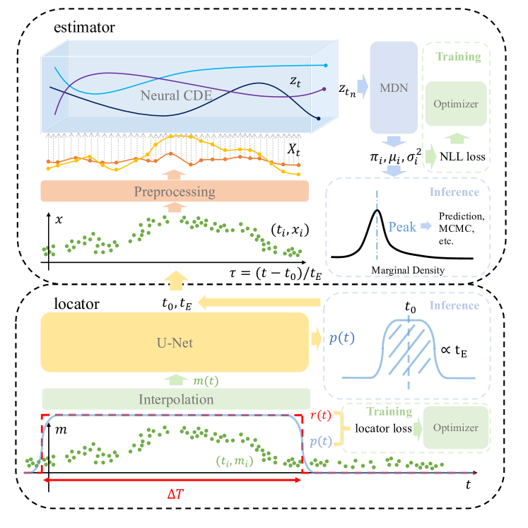
In this paper, we present Microlensing Analysis Guided by Intelligent Computation, or MAGIC for short. MAGIC is a machine learning framework that can efficiently and accurately perform parameter inference in binary microlensing events with realistic sampling conditions. A schematic overview of the proposed framework is shown in Figure 1. The binary microlensing parameters are explained in Section 2. We divide these parameters into two groups and develop different machine learning methods in Sections 3 and 4. Section 5 describes the joint pipeline and its application to a real microlensing event. Finally, we discuss our results in Section 6.
2 Binary Microlensing Parameters
We describe the parameters that are required to model the binary microlensing events. These parameters are grouped and inferred separately.
The standard binary microlensing light curve can be defined by the following parameters (see Gaudi 2012 and references therein)
| (1) |
Here is the time of the closest approach between the source and lens under the rectilinear trajectory, is the separation between the source and the lens at , is the size of the source star, and is the event timescale
| (2) |
where is the relative proper motion between the lens and the source. The Einstein ring radius is given by
| (3) |
where , , with and the mass of and distance to the lens object/system, respectively, and the distance to the source. Both and are normalized to the Einstein radius .
Three of the remaining parameters, , characterize the binary component. Here is the mass ratio between the secondary and the primary components, is the projected separation between the two binary components normalized to , and measures the angle from the binary axis to the direction of the lens–source relative motion. We follow the convention of Skowron et al. (2011) in the definition of the microlensing parameters except for , for which our definition is offset by . 111This is the same in MulensModel (Poleski & Yee, 2019).
The baseline magnitude of the microlensing light curve is given by , and the fraction of the total baseline flux coming from the microlensing source is given by . That is,
| (4) |
where is the light curve in microlensing magnifications. The quantity, , represents the blending fraction, namely the fraction of total flux coming from stars/objects other than the source. The parameters and measure the displacement from the center of mass of the binary (i.e., the chosen origin) to the source at time . In the chosen reference frame,
| (5) |
In principle, since microlensing observations are usually taken by telescopes at different sites or in different filters, each event may have multiple sets of and parameters. In practice, as long as the different datasets cover a broad range of microlensing magnifications, they can all be aligned to a single dataset to relatively high precision without reference to specific microlensing models (e.g., Yoo et al., 2004; Gould et al., 2010a). We therefore only include one set of and in the present work.
The binary microlensing parameters, given by Equation (1), are treated/inferred differently in the present work. First of all, it is reasonable to assume that the baseline magnitude can be immediately read out of the ground-based light curve, which usually monitors (or can monitor) the source star for a time much longer than the event timescale. We therefore do not include in our method. The scaled source size, , is constrained only when the source is very close to or crosses the caustic curve of the binary lens. For the chosen (effective) observational cadence of this work, the finite-source effect is not expected to be widely detected. We therefore fix and do not infer it. As will be shown later, our inference of the other parameters is not affected by whether or not the finite-source effect is present.
Of the remaining parameters, and define the position and extent of the light curve in time, whereas the other parameters, , concern primarily the shape of the binary microlensing light curve. We show in Sections 3 and 4 that these two groups of parameters can be inferred separately. It is also worth noting that, once the other parameters are chosen, the source flux parameter, , can be derived analytically via the maximum likelihood method (Gould, 1995). In Section 4, we make use of this property in the further optimization of the microlensing parameters.
3 Inference of time-dependent parameters
3.1 Method
Together with , parameters and are the so-called Paczynski parameters (Paczynski, 1986). Unlike the parameters that define the binary properties, these Paczynski parameters are constrained by the global properties of the light curve. In many low- events, especially planetary events, one can accurately constrain the Paczynski parameters by masking out the relatively brief anomalous features (e.g., Gould & Loeb, 1992). Of all three Paczynski parameters, the time-dependent ones, namely and , enter the microlensing phenomenon via the parameter (see Equation 5). For these reasons, we develop a stand-alone machine learning method to infer the time-dependent parameters, which is dubbed locator.
The basis of locator is the U-Net architecture. U-Net is a fully convolutional neural network that is originally designed to perform semantic segmentation of images (Ronneberger et al., 2015). U-Net takes the original image as the input, and outputs a mask of the same shape. The mask can be interpreted as a pixel-wise classification result, representing, for example, the probability of each pixel belonging to some specific segment. U-Net has been ubiquitously used in biomedical image processing (Siddique et al., 2021) since it was proposed in 2015. It has also seen a growing number of applications in astronomy (e.g., Van Oort et al., 2019; Makinen et al., 2021).
The architecture of our locator closely follows that of (Ronneberger et al., 2015). See their Figure 1 for an illustration. In details, locator differs in three aspects. First, all convolutional layers are one dimensional, because locator deals with time series data rather than image data. Second, the pure convolutional blocks are replaced by residual blocks (He et al., 2016) with Parametric Rectified Linear Unit (PReLU, He et al. 2015) activation functions to ease gradient back-propagation. Third, we set the channel and kernel sizes to be 128 and 7, respectively, to better match the shape of the input data. In practice, the performance of locator is not sensitive to the values of these hyper-parameters.
We design locator to identify the light curve segment that falls within a predefined time window . Here is a parameter that can be tuned to optimize the output performance, and its choice will be discussed in Section 3.3. For each light curve, which is irregularly sampled (see Section 3.2), we first interpolate it with natural cubic splines and extract the values at 222This value of is chosen to be larger than the number of time stamps (2000, see Section 3.2). The resulting time resolution, days, is much smaller than the RMSE (2.2 days, see Section 3.3) of . equally stepped time stamps . 333This crude approach of directly interpolating the irregular time series is justified given that the temporal parameters depend mostly on the macroscopic behaviour of the light curve, rather than the fine structure within a small time interval. This assumption is no longer valid for the parameters discussed in Section 4. These time stamps are assigned labels depending on whether or not they are inside ,
| (6) |
At run-time, locator takes the time series and attempts to produce a mask that best approximates the ground truth labels.
We train locator on simulated light curves that match the key properties of real microlensing light curves (see Section 3.2). The loss function that locator minimizes is given by
| (7) |
Here is the binary cross entropy (BCE) loss function
| (8) |
which is the standard loss function for binary classification (Goodfellow et al., 2016). The expectation runs over all time stamps of all light curves in the training set. The second term in Equation (7) is the Dice loss function (Sudre et al., 2017), which is introduced to assuage the class imbalance problem in events with small :
| (9) |
The third term in Equation (7) is the regularization term to prevent the mask from wiggling up and down for more than twice
| (10) |
The expectations in the last two terms are performed on all light curves in the training set.
The output mask from locator contains information about the event peak time, , and the timescale, . Specifically, the centroid of the mask corresponds to and the total enclosed area is directly related to . In the continuum form, they are given by
| (11) |
These integrals are evaluated via the trapezoidal rule in the discrete time series.
3.2 Data generation
To simulate light curves for the training of locator, we randomly sample 2000 time stamps out of a total duration of days. This corresponds to an averaged cadence of hr, with the lower and upper 10th percentiles corresponding to 20 min and 7.2 hr. For each light curve, we randomly draw from a truncated log-normal distribution with mean of days, standard deviation of days, and boundaries at 5 and days. This log-normal distribution matches approximately the observed distribution of (e.g., Mróz et al., 2017), and the truncations are introduced to eliminate relatively short-timescale and long-timescale events, both of which may be subject to additional issues (e.g., parallax effect for long events) and are not the focus of the present work. As for , even though it can be any value during (and possibly outside) the sampled time interval, it is reasonable to believe that a very rough by-eye estimate can limit to within of the truth. We therefore randomly draw out of a uniform distribution between and . To summarize,
Although the goal of locator is to infer and and not the other parameters, the training data set should be representative of the target—the binary light curves. We therefore sample the remaining parameters in the following way
and is fixed at , given that the finite-source effect is not expected to be detected for the adopted (effective) cadence. Note that the mass ratio is limited to simply because we want to focus on relatively massive binaries. With increased sampling cadence locator can in principle be extended down to lower values. We defer a detailed exploration to future works.
With the sampled binary parameters and time stamps, we calculate the microlensing light curve using the VBBL algorithm (Bozza, 2010; Bozza et al., 2018). To introduce noises to the simulated light curves, we adopt a simplified noise model. Gaussian noises with signal-to-noise ratios (S/N) of 33 in flux are assumed for all data points, and the flux values are converted to magnitudes for a baseline object with .
Simulated light curves without significant binary features, defined as /d.o.f. , 444Here “pspl” represents for point-source point-lens. are rejected. In the end, two data sets each containing light curves are generated, one for training and the other for validation and test.
3.3 Performance of locator
For our default run, we set so that with the longest timescale (days) can still be fully covered in the simulation interval . We train locator with the ADAM optimizer (Kingma & Ba, 2014). The learning rate is set to initially and drops by ten percent after each epoch. Training samples are divided into mini-batches of size 128. After 13 epochs (2 hours) of training on one NVIDIA Tesla V100 GPU, the average loss drops to 0.16 on the validation set of size 1024. The optimized model is then used to predict the mask and estimate and according to Equation (11).
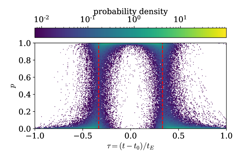
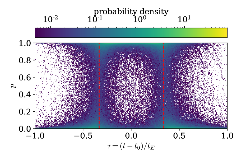
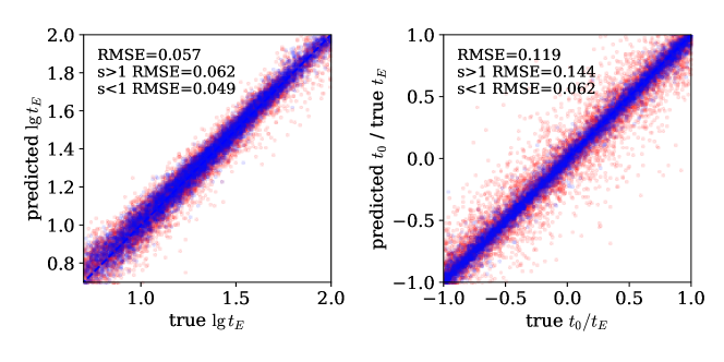
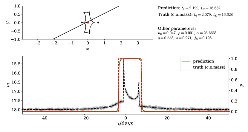
We evaluate locator on 16,384 light curves from the test set. The output masks are illustrated in Figure 2 and Figure 3, and the comparisons between the predicted and ground truth values of and are shown in Figure 4. The accuracy of the prediction is measured by the root-mean-squared error (RMSE) between the ground truth and the prediction. They are indicated in the upper left corner respectively. We note that locator has very different performances on close () binaries and wide () binaries. This is especially true for the parameter. We take the results of close binaries as a more reliable evaluation of the overall performance and defer to the end of this section a more detailed explanation of this phenomenon.
In the default run, locator achieves an accuracy in with RMSE, which translates to a fractional uncertainty of on . The accuracy on the ratio is comparable at RMSE()=0.062, which corresponds to an uncertainty of days on for a typical event with days. An example event is shown in Figure 5, in which the light curve substantially deviates from the Paczynski (1986) model due to the caustic crossing feature and yet locator successfully recovers and at high accuracy.
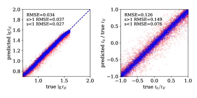
As shown in the left panel of Figure 4, the scattering in increases for shorter events. This is probably because, as timescale decreases, fewer data points are available to locator in the parameter inference. For example, with there are only time stamps fall within for the shortest (days) event. To improve the performance of locator on short events, we select light curves with days and train another model with . After 8 epochs of training with the same learning rate schedule, the loss drops to 0.083 on the validation set. We evaluate the new model on 16,384 light curves with days. 555This includes light curves used in Figure 4 with and additional ones in the test set that add up to 16,384. The results are shown in Figure 6. The prediction accuracy on the timescale increases by a factor of , reaching a fractional uncertainty on of . The performance on the ratio remains largely unchanged.
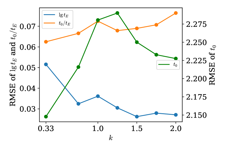
The above investigation has two implications. First, it outlines a general strategy to obtain more accurate . For example, one may divide the overall range of into multiple smaller intervals and train separate locator models. The preliminary estimate of from the default run of locator can then be “polished” by the locator model that is optimized for the narrower interval including the preliminary estimate. Additionally, the comparison in locator performance between two values also sheds light on how locator works. In the single-lens case, the most constraining power on comes from the central region with width of , whereas the event timescale is best constrained by data points extending into the light curve wings. This seems to apply to locator as well. As shown in Figure 8, the timescale parameter can be better constrained when a wider mask window (i.e., a larger ) is used, whereas the event peak time is largely unaffected by the choice of . More works are needed to better understand the mechanism of locator (and U-Net in general).
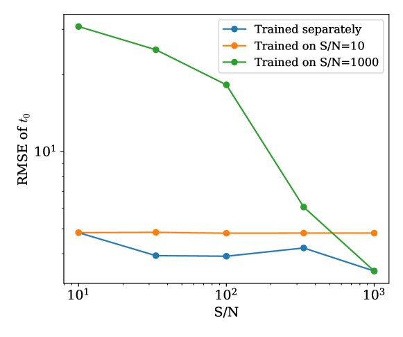
We have fixed the magnitude of the baseline object at 18 and used S/N=33 for all data points in all simulated events. In reality, the baseline magnitude varies from event to event, and the photometric uncertainty varies from data point to data point. However, as discussed previously, the choice of the baseline magnitude does not really matter to the performance of locator, as long as the photometric observations cover a long enough time baseline. We therefore only focus on the impact of varying S/N on the performance of locator. Rather than simulating the realistic noise conditions, 666In real applications, one can and should preprocess the original light curve via, for example, outlier removal and data point rebinning, to make its data quality similar to that of simulated light curves. we study the impact of different training strategies. Several datasets with different S/N values are generated following the method in Section 3.2. We then train locator models on light curves with a fixed S/N value and then evaluate the performance on light curves from the same dataset. The result of this training strategy is shown as the blue points in Figure 9. Here we only show the RMSE values of as the trend is very similar for . Next, we train one locator model on events with the lowest quality (S/N=10) and apply it to all datasets, the result of which is shown in orange in Figure 9. In the third test, we train locator on events with the highest quality (S/N=1000) and apply it to all datasets. This result is shown in green in the same figure. As expected, locator performs the best if it is trained and evaluated on light curves with the same (or very similar) data quality. However, the performance of locator is only slightly worse if it is trained on the noisest dataset. This is probably because locator, similar to other convolutional neural networks (Goodfellow et al., 2016), is effectively composed of a series of filters learned from the data. When faced with noisy data, it learns to denoise through training, so the relatively large noises in the training data make locator more robust. For the same reason, the accuracy of the predicted is substantially worse on noisy light curves if locator only saw during the training light curves of the highest quality. For applications to real events, it seems that training one locator on relatively noisy data may be a good strategy that balances efficiency and accuracy.
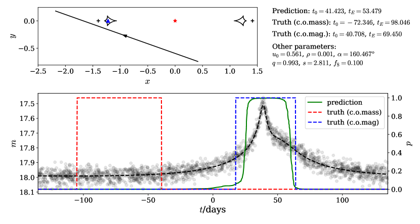
Finally, we discuss the issue related to wide () binaries. As pointed out earlier, the match between the ground truth labels and the predictions of locator for wide binaries is not as good as for close binaries. This larger mismatch, however, does not mean that the inference power of locator is reduced for wide binaries. After visually inspecting a large number of wide binary light curves, we find that the mismatch is related to the use of the reference system. When generating the light curves, we have followed the common convention and adopted the center of mass of the binary as the origin of the coordinate system. However, for wide binaries, the external shear due to a component at wide separation is better modeled in the reference frame defined on the center of magnification. For , the offset between the center of mass and the closer center of magnification is (e.g., Di Stefano & Mao, 1996; Chung et al., 2005; Penny, 2014)
| (12) |
For very wide binaries, the event timescale given by the mass of the closest lens also takes over the timescale given by the total mass of the binary. Both can lead to large offsets between the ground truth window and the predicted window. The most extreme example that has the largest deviation in and with and is shown in Figure 7. Once the reference frame defined on the center of magnification is adopted, the match between the ground truth and the prediction of locator is substantially improved (see also Zhang et al. 2021).
4 Inference of time-independent parameters
4.1 Method
We develop a separate method to infer the time-independent microlensing parameters, which we re-parameterize as
| (13) |
As shown in Figure 1, this estimator consists of two main parts. A neural controlled differential equation (neural CDE) is used to extract features from the microlensing light curve, which is irregularly sampled and may contain large data gaps. The second part, mixture density network (MDN), infers the probability distribution of the microlensing parameters.
To improve the training speed and reduce the memory requirement, we first apply the log-signature transform (Morrill et al., 2021). This transform outputs a shorter, steadier, and higher dimensional sequence that summarizes the sub-step information. For the simulated light curves with 500 time stamps (see Section 4.2), we set the log-signature depth and the shortened length . The output thus has dimensions.
Neural CDE approximates the underlying process of the time series as a differential equation (Kidger et al., 2020; Kidger, 2022)
| (14) |
Here the latent state is defined on the time interval of the input signal, , with dimensions. The continuous signal , defined on the same time interval, is obtained from applying natural cubic splines to the input, discrete signal. 777 Note that the use of cubic splines does not mean that neural CDE is just another interpolation scheme. This is solely for creating a continuous embedding of the discrete input. In contrast, standard interpolation schemes only make use of the values at fixed time stamps. A detailed discussion on this issue can be found in Kidger (2022). The initial value and signal-derivative of the latent state, and , are two different neural networks, where the subscript denotes the dependence on the learnable machine learning parameters. By Equation 14, neural CDE gradually extracts features from the signal according to a learned policy , records its knowledge in the latent state , and output a terminal value that summarizes the useful information of the input signal. We refer interested readers to Kidger et al. (2020) and Kidger (2022) for further details of neural CDE.
The summary features from neural CDE is then fed into the MDN (Bishop & Nasrabadi, 2006) to estimate the probability distribution of the microlensing parameters
| (15) |
Here denotes the density of a multivariate Gaussian with mean and covariance matrix . The normalized weight , mean , and covariance matrix of each of the multivariate Gaussians are given by the neural network of MDN. Compared to the masked autoregressive flow method of Zhang et al. (2021), MDN provides a straightforward and efficient alternative with explicit density estimation, which is useful for the identification of degenerate solutions and the further optimization (see below). We adopt Gaussians with diagonal covariance matrices. This preserves universality as long as is large enough (Bishop & Nasrabadi, 2006).
In the joint framework, estimator, the initial value network , the evolution network , and MDN are constructed as residual networks (ResNet, He et al. 2016) with three residual blocks and each block consisting of two fully connected layers of width 1024. The evolution network has an additional activation of hyperbolic tangent to rectify the dynamic. To train the model, we minimize the negative log-likelihood (NLL) loss function
| (16) |
To further optimize the microlensing parameters, we start from mean positions of the multivariate Gaussians and minimize the light curve values via the Nelder & Mead (1965) simplex algorithm. In this step, the source flux parameter is derived analytically for a given set of by maximizing the model likelihood (e.g., Poleski & Yee, 2019).
4.2 Data generation
For the purpose of learning the time-independent parameters, we generate light curves as functions of the parameter . This is equivalent as setting and d. The other parameters are sampled in the same way as in Secion 3.2.
Each light curve contains 500 data points randomly drawn within the interval . For a typical timescale d, this corresponds to an averaged cadence of 4 hr with a range from 24 min (lower 10%) to 8.8 hr (upper 10%). To mimic the missing data points due to bad weather and/or instrumental failures, we throw away data points within one randomly chosen light curve segment out of the 25 equal-duration segments that constitute the whole light curve. This leaves a data gap of d for the aforementioned timescale. Light curves and noises are generated in the same way as in Section 3.2. Finally, we only keep light curves with significant binary features, defined as /d.o.f. .
Six data sets are generated, each having light curves. We use five of them for training estimator and the last one for validation and test. To further understand the performance of estimator on light curves with different cadences, we have also generated data sets with various numbers of data points within the interval . For these additional data sets, we have assumed irregular sampling but no gap.
4.3 Performance of estimator
We train estimator with the ADAM optimizer (Kingma & Ba, 2014). The learning rate, initially set to , drops by ten percent after each epoch and reaches a minimum of . Training samples are labeled by their input parameters and divided into mini-batches of size 128. The training took day for 50 epochs on one NVIDIA Tesla V100 GPU, and the average loss drops to on the validation set of size 1024.
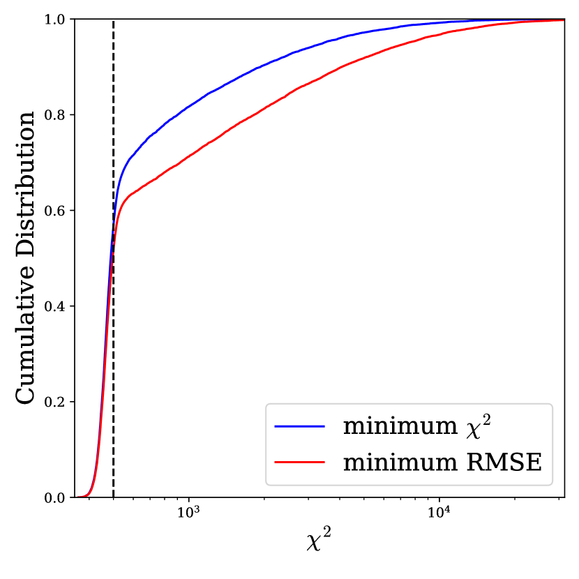
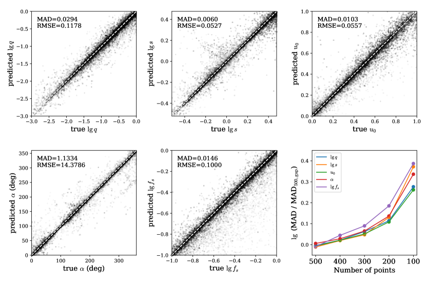
We apply the optimized estimator to 16,384 light curves from the test set and obtain the probability distribution of the microlensing parameters given by the summation of 12 multivariate Gaussians. We then apply the Nelder & Mead (1965) simplex algorithm to get the refined microlensing parameters. We show in Figure 10 the cumulative distributions of the model values of two selected sets of parameters, one that has the smallest value and the other that is closest to the input position in the parameter space. The median values are for both solutions, comparable to the number of data points in the simulated light curve and thus approximately the degrees of freedom. This suggests that the found solutions can indeed describe the data very well. Even though in 20%–30% of cases the model values are substantially large compared to the number of data points, the returned parameters are still good representatives of the input parameters, as will be discussed later. Appendix A shows an example event whose model prediction gives large and yet reasonably accurate binary parameters.
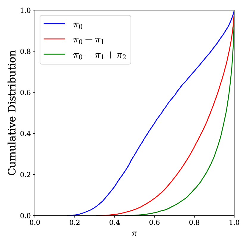
We have included a mixture of Gaussians in the density estimate. Is it flexible enough? To answer this question, we first look at the distribution of the Gaussian weights given by estimator. As shown in Figure 11, the probability distribution is dominated by one Gaussian in 50% of the tested events and by the top three Gaussians with the highest weights in nearly all tested events. As for the optimized solutions, 74% and 85% of the minimum and minimum RMSE solutions are given by the top four Gaussians, respectively. Only in of the tested events does the Gaussian with the lowest weight lead to either solution. Therefore, we conclude that 12 Gaussians can satisfactorily describe the probability distribution of microlensing model parameters.
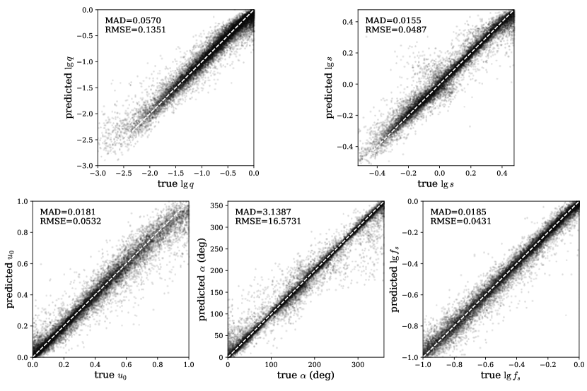
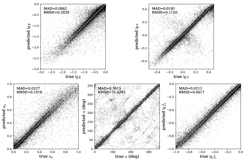
We compare the estimator predictions before and after the simplex optimization with the input parameters in Figures 12 and 13. For each tested event, we choose as the model prediction the set of parameters that is closest to the input position in the parameter space, in order to minimize the impact of degenerate solutions. The results change only marginally if we pick the Gaussian with the highest weight as the model prediction, as seen in Figure 14. We use the median absolute deviation (MAD) to evaluate the agreement between input and prediction. Compared to RMSE, MAD is more robust against outliers. As shown in Figure 12, the direct output of estimator already contains a set of parameters that is fairly close to the input truth. Among all parameters, binary mass ratio and separation are of special interest to the physical interpretation of the event. The direct output of estimator yields a typical deviation of () for (), corresponding to a fractional uncertainty of () on (). The accuracy of the prediction is further improved after the optimization, as shown in Figure 13. Specifically, the optimized prediction can achieve median deviations of and for and , corresponding to fractional errors of and in and , respectively. Overall, the agreement between the input and predicted values is very well, demonstrating the high accuracy of our method on light curves with realistic sampling conditions.
We have also applied the optimized estimator to light curves in the additional data sets, which have different averaged cadence but no data gap. 888That is, we directly apply estimator without retraining. The results are shown in the lower right panel of Figure 13 for the optimized prediction. There are a few interesting trends to report. First, the performance of estimator is better, although fairly marginally, on events with 500 points and no data gap. Second, the prediction accuracy decreases with decreasing number of data points as expected, but the degradation is typically small. Specifically, with 200 data points the prediction accuracy is only worse by compared to the default case with 500 data points. The only exception is seen in the case with 100 data points, for which the performance is reduced by a factor of . This is probably because the averaged cadence becomes too low to constrain binaries with mass ratios down to . 999The averaged cadence in terms of is , and thus the smallest binary mass ratio that it can detect is . Nevertheless, the overall uncertainty in the case of 100 points remains fairly small and acceptable. These results may provide useful guidance to the future application of our method to real light curves with variant cadences and/or the detection of low mass-ratio planets.
We show in Figure 15 an example event whose anomalous feature is only partially covered by data points. The probability distribution from estimator, represented by the multivariate Gaussians, is already at the neighborhood of the ground truth position. The optimization with Nelder & Mead (1965) algorithm leads to even better match in microlensing parameters as well as model the light curve. Events like this one, which have irregular samplings and large data gaps, pose challenges to machine learning methods that base on the standard RNN approach.
Our method also identify multiple solutions in events that suffer model degeneracy. We defer to Section 5.2 for further discussions on this issue.
5 Joint Pipeline & Real Event Application
5.1 Joint pipeline
Combining the methods described in Sections 3 and 4, the joint pipeline of MAGIC works as follows. First, we feed the light curve into locator, which outputs the predicted and . If is small, we can further refine it using locator with a larger . Then we use the predicted and to shift and rescale the light curve. The resulting light curve is processed by estimator, which in return gives the positions and shapes of Gaussians in the parameter space. If needed, these Gaussians can be further optimized to obtain more accurate prediction or predictions (see Section 4.1).
The performance of the combined pipeline is largely determined by the propagation of inaccurate parameters from locator to estimator. We therefore test the joint pipeline on 16,384 light curves from the test set of locator. After applying locator, we transform the light curves using the predicted values of and . The transformed light curves are then sent to estimator to infer the time-independent microlensing parameters. The set of parameters closest to the position of the input values in the parameter space is adopted as the final prediction.
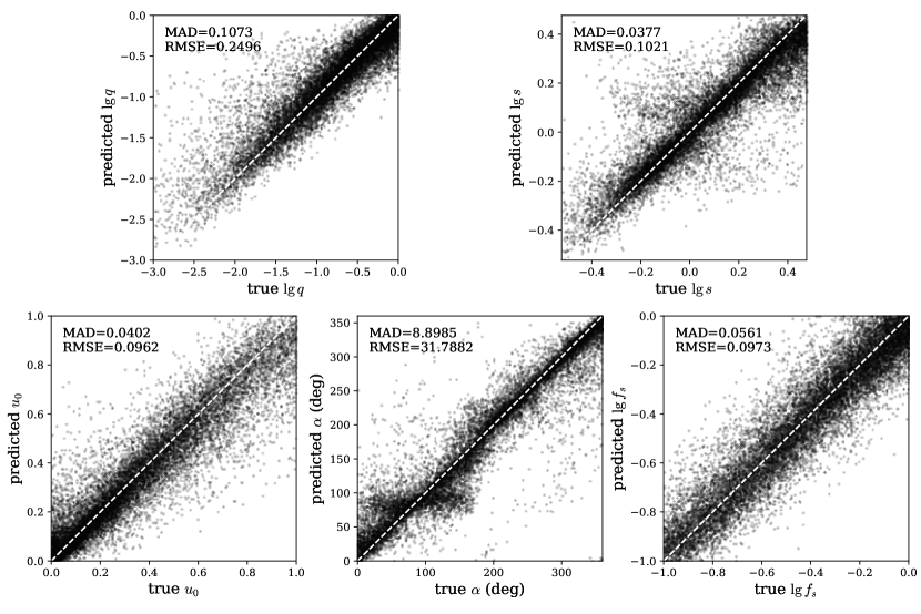
The comparisons between the input and the predicted values of the time-independent parameters are shown in Figure 16. The typical, fractional deviation in and are and , respectively. These deviations remain small, even though they are worse than the estimator-only case by a factor of . Overall, the joint pipeline achieves fairly high prediction accuracy in the time-independent parameters even with the use of the inaccurate time-dependent parameters. We expect the accuracy to be further improved once the predictions are optimized via the Nelder & Mead (1965) algorithm, as seen in the estimator-only case.
A substantial fraction of binary events can be well described by a Paczynski (1986) model plus relatively short binary perturbation. For such events, one may mask out the anomalous feature and fit a single-lens model to obtain precise and accurate peak time and event timescale . Combining these values with estimator, we can achieve nearly as accurate time-independent parameters as we do in the estimator-alone case.
It is worth noting that the light curves generated for locator are similar to but not the same as those used for training estimator. First, locator uses binary light curves with , whereas estimator uses binaries with . Both correspond to a between single and binary models, under the reasonable assumption that the binary signals are usually local features. 101010Although we have focused on such binaries with strong signals, we expect our method to work on weak binaries as well. Furthermore, the time window is fixed and the timescale parameters varies in the data set for locator. This means the number of data points within varies too. Nevertheless, we have shown in Section 4.3 that the performance of estimator is only mildly affected with the various length of input time series.
In addition to its high accuracy, our method demonstrates high efficiency in the parameter estimation. Specifically, locator and estimator can process and light curves per second on a single GPU, respectively. As shown in Figure 13, the output of estimator is already accurate enough for purposes like statistical studies. If needed, the optimization step can be performed. Compared to the two machine learning steps, this traditional optimization step is slower, but there are only up to 12 initial positions to be optimized, which altogether may require up to a few thousand light curve evaluations. For comparison, the traditional approach usually requires optimizations at individual grid points on a fine grid in the space (e.g., Albrow et al., 2000; Wang et al., 2022). Our approach therefore represents a speedup by factors of –.
5.2 A Real Event Application
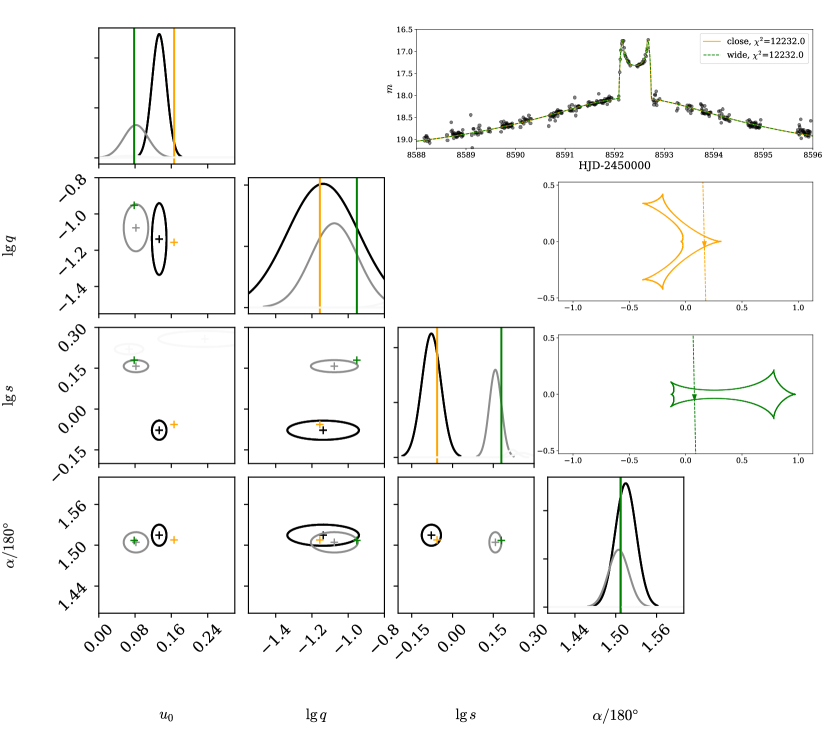
We apply MAGIC to KMT-2019-BLG-0371 (hereafter KB190371 for short), which is a short-timescale (d) binary event with or (Kim et al., 2021). KB190371 is chosen for this demonstration based on several considerations. First, its caustic-crossing feature is prominent and U-shaped, which is typical for binary events. Second, this event suffers from the close/wide degeneracy (Griest & Safizadeh, 1998; Dominik, 1999) 111111We use this term to keep consistent with the original discovery paper, even though recent studies have suggested that such “close/wide degeneracy” should be called offset degeneracy (Zhang et al., 2022) , thus enabling additional tests of MAGIC. Furthermore, except for the relatively short timescale, the other microlensing parameters are fairly typical in comparison to those used in our simulation.
The available data sets from Kim et al. (2021) are not aligned to the same magnitude system. In order to align the data sets and then apply MAGIC, we mask out the caustic-crossing feature, fit a Paczynski (1986) model to the data, and use the best-fit flux parameters to align all other data sets to the OGLE one. We note that, although here we have made use of the special property of KB190371 to align the data sets, such a data alignment task is the same as deriving the source color and can be performed without reference to specific microlensing models (Yoo et al., 2004; Gould et al., 2010a), as has been practiced in the analysis of many real microlensing events (e.g., Gould et al., 2010b; Zhu et al., 2017).
To apply our joint pipeline, we first preprocess the data and make the light curve similar to those used in the training procedure. To be more specific, we only include data points falling in the time interval of about 100 days centered at the anomaly, and filter out data points with large (mag) error bars. KB190371 was observed with high cadence, so we bin every five consecutive points into one. Finally, the light curve is shifted to the same base magnitude as those used in locator.
Then we feed the preprocessed light curve into locator. Because the timescale is relatively small, we set . The output mask is rectified into binary values with a threshold of . This step gives the prediction and d, both of which are close to the values given in Kim et al. (2021). We transform the light curve with the predicted and and only keep the segment within .
The rest of application follows closely the procedure given in Section 5.1. With the positions of the 12 multivariate Gaussians given by estimator, we perform Nelder & Mead (1965) optimization to further refine the microlensing parameters. Because the light curve shows prominent finite-source effect, we also include in the optimization the scaled source size .
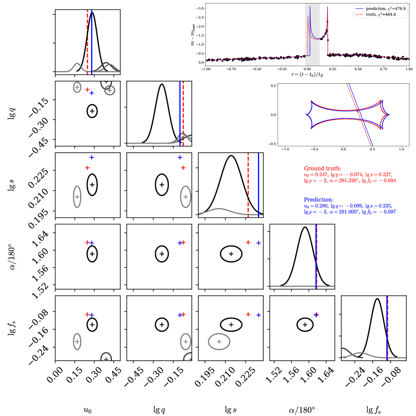
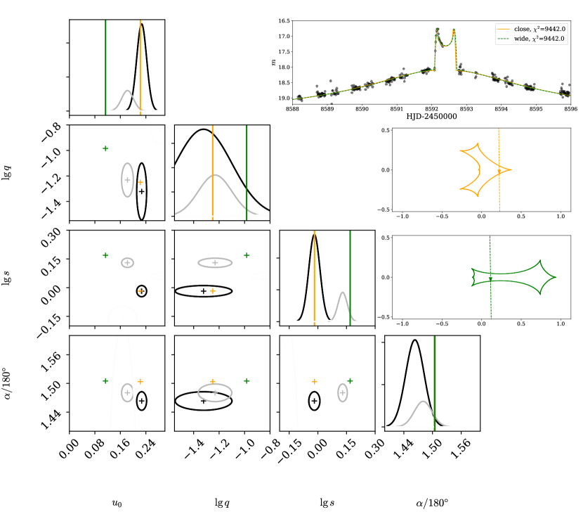
The results are shown in Figure 17. The top two Gaussians with the highest weights match closely to the close () and wide () solutions, respectively. The corresponding model light curves from the optimized solutions both match the data reasonably well, with almost indistinguishable values. According to these solutions, the event can be explained by a binary with or . Given the imperfect alignment as well as the slightly different preprocessing procedures, we consider these values in good match with those given by the discovery paper.
Kim et al. (2021) found the source scaled parameter to be and for the close and wide solutions, respectively. These are quite different from the value () that we have used to train MAGIC. Nevertheless, the optimized parameters yield and for the close and wide solutions, respectively, in good agreement with the values from the discovery paper. In other words, the presence of the finite-source effect in KB190371 does not seem to confuse MAGIC, even though MAGIC has not learned to infer the source scaled parameter . This is probably because the finite-source effect in KB190371 only affects a limited number of data points around the caustic entrance and exit. While the majority of binary microlensing events bear the same feature, some may have their binary signals substantially modified by the finite-source effect (e.g., Hwang et al., 2018). Therefore, it may be necessary to include in MAGIC the ability to infer . See Section 6 for further discussion.
To further demonstrate the capability of MAGIC to handle large data gaps, we exclude observations from the South Africa site of KMTNet. This creates a substantial gap during the exit of the caustic crossing, as shown in the top right panel of Figure 18. The same procedure is applied as before, and the results are shown in Figure 18. The two degenerate solutions are again identified at high accuracy, indicating the robustness of MAGIC in handling large data gaps as well as model degeneracy.
6 Discussion
We present Microlensing Analysis Guided by Intelligent Computation (MAGIC), a machine learning method that is readily applicable to the analysis of binary microlensing light curves from ongoing and future photometric surveys. We divide the microlensing model parameters into two groups and develop separate deep learning neural networks. For the inference of time-dependent parameters, namely the peak time and the event timescale , we construct locator, which is a U-Net architecture (Ronneberger et al., 2015). For the inference of time-independent parameters, namely , we construct estimator, which uses neural CDE (Kidger et al., 2020; Kidger, 2022) to extract features and mixture density network (MDN; Bishop & Nasrabadi 2006) to infer the probability distribution. The output parameters can be further refined through the standard optimization method. Depending on properties of the event under investigation, the two components can be used separately or jointly to achieve the best performance.
A little MAGIC can take you a long way. 121212From Roald Dahl. We train and validate both locator and estimator as well as the joint pipeline on simulated light curves. To mimic the sampling condition in the realistic world, we introduce irregular sampling and large data gap in the light curve simulation. As demonstrated in previous sections, MAGIC can recover the input parameters at high accuracy for the majority of tested events. In particular, estimator alone can achieve typical fractional errors of and for the binary mass ratio and the separation , respectively. As demonstrated in the analysis of a real microlensing event (KB190371; Kim et al. 2021), MAGIC is also capable of identifying degenerate models that explain the same data. The proposed method is fast to perform, with an estimated speedup of – depending on whether or not the optimization is needed.
While MAGIC is readily applicable to the analysis of real world data sets, a few improvements can be made to make MAGIC more powerful and more robust. First, this work focuses on binaries with relatively large mass ratios (), and extension into lower values may be necessary in order to apply MAGIC to the analysis of low-mass planetary events. Second, the source scaled size is not inferred in the current version of MAGIC for reasons given in Section 3.2, although it can still be constrained in the optimization stage (see Section 5). The inclusion of into MAGIC involves effectively both classification and regression tasks, as one will need to determine whether or not the finite source effect is detected and if yes, infer the value of . Furthermore, the inclusion of additional effects—especially the microlensing parallax effect (Gould, 1992) and the binary source effect (Griest & Hu, 1992)—may be necessary in order for MAGIC to provide robust estimates on binaries with relatively weak signals. Last but not least, MAGIC can also be applied to the analysis of microlensing events with more than two lenses, for which the sampling-based method becomes much more time-consuming (e.g., Gaudi et al., 2008; Kuang et al., 2021).
MAGIC uses neural CDE to handle irregular sampling and data gaps. Compared to other existing methods that have been used to handle the same issues in astronomical time series (e.g., Charnock & Moss, 2017; Naul et al., 2018), neural CDE takes directly the irregularly sampled time series and models the underlying process with a differential equation. This approach has been demonstrated to achieve good performances in other disciplines that also involve time series data (e.g., Kidger et al., 2020). As irregular sampling and data gaps are common in astronomical observations, we expect that neural CDE will be useful to many other fields in time domain astronomy.
Appendix A Events with Large
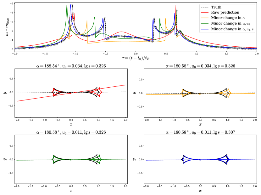
As described in Section 4.3, estimator achieves reasonably high accuracy in microlensing parameters but fails to obtain good light curve fits (i.e. small values) in of the test cases. This phenomenon arises because a small deviation in the parameter estimation may still lead to a large deviation in the light curve behavior, thus resulting in a large value. Here we examine a specific example, which is the event with the largest value in the test set. The predicted parameters only differ from the ground truth values by in . However, the corresponding light curve deviates from the ground truth drastically, as shown by the red curve in the top panel of Figure 19. To illustrate the impact on the light curve behaviour caused by minor changes in the parameter values, we change one-by-one the values of , , and from the model prediction to the ground truth values, and plot the corresponding light curves in the same figure. We observe that the light curve fit remains bad until all the three parameters are fine tuned. This confirms that even when the parameter estimation is accurate enough, the light curve fit may still looks bad. Nevertheless, an accurate estimation of the parameters is enough for most applications.
References
- Albrow et al. (2000) Albrow, M. D., Beaulieu, J. P., Caldwell, J. A. R., et al. 2000, ApJ, 535, 176, doi: 10.1086/308842
- An (2005) An, J. H. 2005, MNRAS, 356, 1409, doi: 10.1111/j.1365-2966.2004.08581.x
- Bishop & Nasrabadi (2006) Bishop, C. M., & Nasrabadi, N. M. 2006, Pattern recognition and machine learning (Springer)
- Bozza (2010) Bozza, V. 2010, MNRAS, 408, 2188, doi: 10.1111/j.1365-2966.2010.17265.x
- Bozza et al. (2018) Bozza, V., Bachelet, E., Bartolić, F., et al. 2018, Monthly Notices of the Royal Astronomical Society, 479, 5157, doi: 10.1093/mnras/sty1791
- Charnock & Moss (2017) Charnock, T., & Moss, A. 2017, Astrophysical Journal Letters, 837, L28, doi: 10.3847/2041-8213/aa603d
- Che et al. (2018) Che, Z., Purushotham, S., Cho, K., Sontag, D., & Liu, Y. 2018, Scientific reports, 8, 1
- Chung et al. (2005) Chung, S.-J., Han, C., Park, B.-G., et al. 2005, ApJ, 630, 535, doi: 10.1086/432048
- Di Stefano & Mao (1996) Di Stefano, R., & Mao, S. 1996, ApJ, 457, 93, doi: 10.1086/176713
- Dominik (1999) Dominik, M. 1999, A&A, 349, 108. https://arxiv.org/abs/astro-ph/9903014
- Dong et al. (2006) Dong, S., DePoy, D. L., Gaudi, B. S., et al. 2006, ApJ, 642, 842, doi: 10.1086/501224
- Einstein (1936) Einstein, A. 1936, Science, 84, 506, doi: 10.1126/science.84.2188.506
- Foreman-Mackey (2016) Foreman-Mackey, D. 2016, The Journal of Open Source Software, 1, 24, doi: 10.21105/joss.00024
- Gaudi (2012) Gaudi, B. S. 2012, Annual Review of Astronomy and Astrophysics, 50, 411
- Gaudi et al. (2008) Gaudi, B. S., Bennett, D. P., Udalski, A., et al. 2008, Science, 319, 927, doi: 10.1126/science.1151947
- Godines et al. (2019) Godines, D., Bachelet, E., Narayan, G., & Street, R. 2019, Astronomy and Computing, 28, 100298, doi: https://doi.org/10.1016/j.ascom.2019.100298
- Goodfellow et al. (2016) Goodfellow, I., Bengio, Y., & Courville, A. 2016, Deep learning (MIT press)
- Gould (1992) Gould, A. 1992, ApJ, 392, 442, doi: 10.1086/171443
- Gould (1995) —. 1995, ApJ, 440, 510, doi: 10.1086/175292
- Gould et al. (2010a) Gould, A., Dong, S., Bennett, D. P., et al. 2010a, ApJ, 710, 1800, doi: 10.1088/0004-637X/710/2/1800
- Gould & Han (2000) Gould, A., & Han, C. 2000, ApJ, 538, 653, doi: 10.1086/309180
- Gould & Loeb (1992) Gould, A., & Loeb, A. 1992, ApJ, 396, 104, doi: 10.1086/171700
- Gould et al. (2010b) Gould, A., Dong, S., Gaudi, B. S., et al. 2010b, ApJ, 720, 1073, doi: 10.1088/0004-637X/720/2/1073
- Griest & Hu (1992) Griest, K., & Hu, W. 1992, ApJ, 397, 362, doi: 10.1086/171793
- Griest & Safizadeh (1998) Griest, K., & Safizadeh, N. 1998, ApJ, 500, 37, doi: 10.1086/305729
- Harris et al. (2020) Harris, C. R., Millman, K. J., van der Walt, S. J., et al. 2020, Nature, 585, 357, doi: 10.1038/s41586-020-2649-2
- He et al. (2015) He, K., Zhang, X., Ren, S., & Sun, J. 2015, arXiv preprint arXiv:1502.01852
- He et al. (2016) He, K., Zhang, X., Ren, S., & Sun, J. 2016, in Proceedings of the IEEE conference on computer vision and pattern recognition, 770–778
- Hunter (2007) Hunter, J. D. 2007, Computing in Science & Engineering, 9, 90, doi: 10.1109/MCSE.2007.55
- Hwang et al. (2018) Hwang, K. H., Udalski, A., Shvartzvald, Y., et al. 2018, AJ, 155, 20, doi: 10.3847/1538-3881/aa992f
- Kennedy et al. (2021) Kennedy, A., Nash, G., Rattenbury, N. J., & Kempa-Liehr, A. W. 2021, Astronomy and Computing, 35, 100460, doi: 10.1016/j.ascom.2021.100460
- Khakpash et al. (2019) Khakpash, S., Penny, M., & Pepper, J. 2019, AJ, 158, 9, doi: 10.3847/1538-3881/ab1fe3
- Kidger (2022) Kidger, P. 2022, arXiv preprint arXiv:2202.02435
- Kidger et al. (2020) Kidger, P., Morrill, J., Foster, J., & Lyons, T. 2020, Advances in Neural Information Processing Systems, 33, 6696
- Kim et al. (2016) Kim, S.-L., Lee, C.-U., Park, B.-G., et al. 2016, Journal of Korean Astronomical Society, 49, 37, doi: 10.5303/JKAS.2016.49.1.037
- Kim et al. (2021) Kim, Y. H., Chung, S.-J., Yee, J. C., et al. 2021, AJ, 162, 17, doi: 10.3847/1538-3881/abf930
- Kingma & Ba (2014) Kingma, D. P., & Ba, J. 2014, arXiv preprint arXiv:1412.6980
- Kluyver et al. (2016) Kluyver, T., Ragan-Kelley, B., Pérez, F., et al. 2016, in Positioning and Power in Academic Publishing: Players, Agents and Agendas, ed. F. Loizides & B. Scmidt (IOS Press), 87–90. https://eprints.soton.ac.uk/403913/
- Kuang et al. (2021) Kuang, R., Mao, S., Wang, T., Zang, W., & Long, R. J. 2021, MNRAS, 503, 6143, doi: 10.1093/mnras/stab509
- Makinen et al. (2021) Makinen, T. L., Lancaster, L., Villaescusa-Navarro, F., et al. 2021, J. Cosmology Astropart. Phys, 2021, 081, doi: 10.1088/1475-7516/2021/04/081
- Mao & Paczynski (1991) Mao, S., & Paczynski, B. 1991, Astrophysical Journal Letters, 374, L37, doi: 10.1086/186066
- Morrill et al. (2021) Morrill, J., Salvi, C., Kidger, P., & Foster, J. 2021, in International Conference on Machine Learning, PMLR, 7829–7838
- Mróz (2020) Mróz, P. 2020, Acta Astronomica, 70, 169, doi: 10.32023/0001-5237/70.3.1
- Mróz et al. (2017) Mróz, P., Udalski, A., Skowron, J., et al. 2017, Nature, 548, 183, doi: 10.1038/nature23276
- Naul et al. (2018) Naul, B., Bloom, J. S., Pérez, F., & van der Walt, S. 2018, Nature Astronomy, 2, 151, doi: 10.1038/s41550-017-0321-z
- Nelder & Mead (1965) Nelder, J. A., & Mead, R. 1965, Comput. J., 7, 308
- Paczynski (1986) Paczynski, B. 1986, The Astrophysical Journal, 304, 1, doi: 10.1086/164140
- Paszke et al. (2019) Paszke, A., Gross, S., Massa, F., et al. 2019, in Advances in Neural Information Processing Systems 32 (Curran Associates, Inc.), 8024–8035
- Penny (2014) Penny, M. T. 2014, The Astrophysical Journal, 790, 142
- Penny et al. (2019) Penny, M. T., Gaudi, B. S., Kerins, E., et al. 2019, The Astrophysical Journal Supplement Series, 241, 3, doi: 10.3847/1538-4365/aafb69
- Poleski & Yee (2019) Poleski, R., & Yee, J. C. 2019, Astronomy and Computing, 26, 35, doi: 10.1016/j.ascom.2018.11.001
- Ronneberger et al. (2015) Ronneberger, O., Fischer, P., & Brox, T. 2015, in International Conference on Medical image computing and computer-assisted intervention, Springer, 234–241
- Rubanova et al. (2019) Rubanova, Y., Chen, R. T., & Duvenaud, D. K. 2019, Advances in neural information processing systems, 32
- Siddique et al. (2021) Siddique, N., Paheding, S., Elkin, C. P., & Devabhaktuni, V. 2021, IEEE Access, 9, 82031, doi: 10.1109/ACCESS.2021.3086020
- Skowron et al. (2011) Skowron, J., Udalski, A., Gould, A., et al. 2011, ApJ, 738, 87, doi: 10.1088/0004-637X/738/1/87
- Song et al. (2014) Song, Y.-Y., Mao, S., & An, J. H. 2014, MNRAS, 437, 4006, doi: 10.1093/mnras/stt2222
- Sudre et al. (2017) Sudre, C. H., Li, W., Vercauteren, T., Ourselin, S., & Jorge Cardoso, M. 2017, in Deep learning in medical image analysis and multimodal learning for clinical decision support (Springer), 240–248
- Van Oort et al. (2019) Van Oort, C. M., Xu, D., Offner, S. S. R., & Gutermuth, R. A. 2019, ApJ, 880, 83, doi: 10.3847/1538-4357/ab275e
- Vermaak (2003) Vermaak, P. 2003, Monthly Notices of the Royal Astronomical Society, 344, 651, doi: 10.1046/j.1365-8711.2003.06851.x
- Virtanen et al. (2020) Virtanen, P., Gommers, R., Oliphant, T. E., et al. 2020, Nature Methods, 17, 261, doi: 10.1038/s41592-019-0686-2
- Wang et al. (2022) Wang, H., Zang, W., Zhu, W., et al. 2022, MNRAS, 510, 1778, doi: 10.1093/mnras/stab3581
- Wes McKinney (2010) Wes McKinney. 2010, in Proceedings of the 9th Python in Science Conference, ed. Stéfan van der Walt & Jarrod Millman, 56 – 61, doi: 10.25080/Majora-92bf1922-00a
- Wyrzykowski et al. (2015) Wyrzykowski, Ł., Rynkiewicz, A. E., Skowron, J., et al. 2015, The Astrophysical Journal Supplement Series, 216, 12
- Yoo et al. (2004) Yoo, J., DePoy, D. L., Gal-Yam, A., et al. 2004, ApJ, 603, 139, doi: 10.1086/381241
- Zang et al. (2022) Zang, W., Yang, H., Han, C., et al. 2022, arXiv e-prints, arXiv:2204.02017. https://arxiv.org/abs/2204.02017
- Zhang et al. (2021) Zhang, K., Bloom, J. S., Gaudi, B. S., et al. 2021, The Astronomical Journal, 161, 262
- Zhang et al. (2022) Zhang, K., Gaudi, B. S., & Bloom, J. S. 2022, Nature Astronomy, 6, 782, doi: 10.1038/s41550-022-01671-6
- Zhu & Dong (2021) Zhu, W., & Dong, S. 2021, ARA&A, 59, doi: 10.1146/annurev-astro-112420-020055
- Zhu et al. (2014) Zhu, W., Penny, M., Mao, S., Gould, A., & Gendron, R. 2014, ApJ, 788, 73, doi: 10.1088/0004-637X/788/1/73
- Zhu et al. (2017) Zhu, W., Udalski, A., Novati, S. C., et al. 2017, AJ, 154, 210, doi: 10.3847/1538-3881/aa8ef1