Tracing the Top-of-the-atmosphere and Vertical Cloud Structure of a fast-rotating late T-dwarf

Abstract

Only a handful of late-T brown dwarfs have been monitored for spectro-photometric variability, leaving incomplete the study of the atmospheric cloud structures of the coldest brown dwarfs, that share temperatures with some cold, directly-imaged exoplanets. 2MASS J00501994–332240 is a T7.0 rapidly rotating, field brown dwarf that showed low-level photometric variability in data obtained with the Spitzer Space telescope. We monitored 2MASS J00501994–332240 during $\sim$2.6 hr with MOSFIRE, installed at the Keck I telescope, with the aim of constraining its near-infrared spectro-photometric variability. We measured fluctuations with a peak-to-peak amplitude of 1.48$\pm$0.75% in the $J$-band photometric light curve, an amplitude of 0.62$\pm$0.18% in the $J$-band spectro-photometric light curve, an amplitude of 1.26$\pm$0.93% in the $H$-band light curve, and an amplitude of 5.33$\pm$2.02% in the $\mathrm{CH_{4}-H_{2}O}$ band light curve. Nevertheless, the Bayesian Information Criterion does not detect significant variability in any of the light curves. Thus, given the detection limitations due to the MOSFIRE sensitivity, we can only claim tentative low-level variability for 2M0050–3322 in the best case scenario. The amplitudes of the peak-to-peak fluctuations measured for 2MASS J00501994–332240 agree with the variability amplitude predictions of General Circulation Models for a T7.0 brown dwarf for an edge on object. Radiative-transfer models predict that the $\mathrm{Na_{2}S}$ and KCl clouds condense at pressures lower than that traced by the $\mathrm{CH_{4}-H_{2}O}$ band, which might explain the higher peak-to-peak fluctuations measured for this light curve. Finally, we provide a visual recreation of the map provided by General Circulation Models, and the vertical structure of 2MASS J00501994–332240 provided by radiative-transfer models.

1 Introduction

The search for brown dwarf photometric variability started soon after the discovery of the first brown dwarfs (e.g. Bailer-Jones & Mundt 1999; Zapatero Osorio et al. 2003; Caballero et al. 2004; Scholz & Eislöffel 2005). The discovery of high-amplitude, periodic photometric variability in the T2.5 brown dwarf SIMP J013656.5+093347 (Artigau et al., 2009) suggested that weather patterns that evolve with the object’s rotation was the most likely cause of its variability. Although other scenarios are possible (Tremblin et al., 2015), these weather patterns are most likely produced by heterogeneous clouds with different varying thickness and temperatures (Apai et al., 2013), forming spots and bands in the atmospheres of brown dwarfs that evolve with time (Apai et al., 2017).

Up to now, dozens of L, L-T and T brown dwarfs have been monitored for photometric and spectro-photometric variability (Radigan et al. 2014; Metchev et al. 2015; Biller et al. 2018; Vos et al. 2019, among others) with ground-based and space-based facilities. Using ground-based facilities, Radigan et al. (2014) concluded that $39^{+16}_{-14}$% of L9-T3.5 dwarfs show in general higher variability amplitude than other spectral types. Outside the L/T transition, Radigan et al. (2014) inferred that $60^{+22}_{-18}$% of their sample vary with amplitudes of 0.5%-1.6%, concluding that heterogeneous clouds are common among brown dwarfs. Similarly, using the Spitzer Space telescope, Metchev et al. (2015) was able to measure flux variations $>$0.2%, determining that most objects in their sample show low-level variability.

Until now, the majority of brown dwarfs monitored for variability have been mostly photometrically monitored in one or several photometric bands. Although single-band photometric variability traces heterogeneities in the atmospheres of brown dwarfs, it only traces one pressure range of the atmosphere of the object at a time. Spectro-photometric variability monitoring is more powerful than single band monitoring, since it simultaneously traces the variability at different wavelengths, including the broad band, and the different molecular and atomic spectral features in brown dwarf spectra (e.g. $\mathrm{H_{2}O}$ and $\mathrm{CH_{4}}$ bands, or the K I, Na I alkali lines). Thus, using spectro-photometric variability monitoring we are able to trace the atmosphere of brown dwarfs at different pressure levels simultaneously, providing a 3D map of their atmospheres (Yang et al., 2016; Manjavacas et al., 2021). Unfortunately, spectro-photometric variability monitoring is challenging to carry out, since we are limited almost only to space-based facilities. In fact, most of the spectro-photometric data we have in the near-infrared have been acquired with the Hubble Space Telescope (HST), and its Wide Field Camera 3 (WFC3) (e.g. Apai et al. 2013; Buenzli et al. 2012; Lew et al. 2016; Yang et al. 2016; Biller et al. 2018; Manjavacas et al. 2018, 2019; Zhou et al. 2020). From the ground, spectro-photometric monitoring for any given brown dwarf is possible only if multi-object near-infrared spectrographs are used, which are relatively scarce (Manjavacas et al., 2021; Heinze et al., 2021), or if a calibration star is close enough to the target to perform single-slit simultaneous spectroscopic monitoring (Schlawin et al., 2017; Kellogg et al., 2017).

To date, only two late-T brown dwarfs have been monitored for spectro-photometric variability: the T6.5 2MASS J22282889–431026 (Buenzli et al., 2012), and the T8.0 Ross 458c (Manjavacas et al., 2019), both with HST/WFC3. 2MASS J22282889–431026 shows different variability amplitude inside and outside the water band, and phase shifts between its light curves in the $J$- and $H$-bands, and with the water band at 1.40 $\mu$m (Buenzli et al., 2012). Ross 458c also shows tentative phase shifts between the $J$- and $H$-band light curves (Manjavacas et al., 2019). Phase shifts have not been commonly observed in HST bands for L and L/T brown dwarfs, so that may point at important differences in the dynamics-cloud coupling for mid and late T-dwarfs with respect to early T-dwarfs. Thus, a larger sample of late-T dwarfs need to be spectrophotometrically monitored to shed light on the dynamics of these objects.

In this paper we present Keck I/MOSFIRE $J$- and $H$-bands spectro-photometric monitoring for another late-T dwarf, 2MASS J00501994–332240 (T7.0, Tinney et al. 2005), with the aim of increasing the sample of late-T dwarfs with spectroscopic variability monitoring, and shedding light into the atmospheric structure of these objects. 2MASS J00501994–332240 shares its spectral type with some cold directly-imaged giant exoplanets, like 51 Eridani b (Macintosh et al., 2015; Rajan et al., 2017). 2MASS J00501994–33224 serves as an analog to provide insights into the cloud structure of cold giant exoplanets for which high signal-to-noise spectro-photometric data are very limited with the existing instrumentation.

This paper is structured as follows: in Section 2 we introduce the properties of 2MASS J00501994–332240. In Section 3 we provide the details of the Keck I/MOSFIRE monitoring for 2MASS J00501994–332240. In Section 4 we describe the data reduction. In Section 5, we explain how the light curve for the object was produced. In Section 6 we evaluate the correlations between our light curve and effects that might introduce spurious variability in our target’s light curve. In Section 7 we present our results, and their significance. In Section 8 we present a discussion of our results. In Section 9 we provide an interpretation of 2MASS J00501994–332240 light curve according to General Circulation and radiative-transfer models. Finally, in Section 10 we summarize our conclusions.

2 2MASS J00501994–3322402

2MASS J00501994–3322402 (2M0050–3322) was discovered by Tinney et al. (2005), and spectral typed as a T7.0 brown dwarf by Burgasser et al. (2006). Dupuy & Liu (2012) measured a trigonometric parallax for 2M0050–3322 of $\pi$ = 94.6$\pm$2.4 mas. 2M0050–3322 has near-infrared magnitudes of $J$ = 15.928$\pm$0.070, $H$ = 15.838$\pm$0.191, and $K$ = 15.241$\pm$0.185 (Cutri et al., 2003). Filippazzo et al. (2015) determined the fundamental parameters of our target by fitting its IRTF/SpeX spectrum to atmospheric models, which provided an estimation of its $\mathrm{T_{eff}}$ and log g. Integrating its absolute flux calibrated Spectral Energy Distribution, Filippazzo et al. (2015) derived its $\mathrm{L_{bol}/L_{\odot}}$. Finally, using the calculated $\mathrm{L_{bol}/L_{\odot}}$, its radius, and mass were derived from evolutionary models. 2M0050–3322 fundamental parameters are: $\mathrm{log(L/L_{\odot})}$ = -5.39$\pm$0.02, age = 0.500–-10.00 Gyrs, R = 0.94$\pm$0.16 $\mathrm{R_{Jup}}$, log(g) = 4.95$\pm$0.49, $\mathrm{T_{eff}}$ = 836$\pm$71 K, and a mass of 40.34$\pm$25.54 $\mathrm{M_{Jup}}$, confirming that 2M0050–3322 has the characteristics of a field T7.0 brown dwarf. No inclination has been measured for 2M0050–3322.

Radigan et al. (2014) found no significant $J$-band photometric variability for 2M0050–3322, but they provided an upper level of 1.1%. Metchev et al. (2015) found variability on the [4.5] Spitzer channel, but not in the [3.6] channel. Metchev et al. (2015) measured a variability amplitude of 1.07$\pm$0.11 % for 2M0050–3322, and a rotational period of 1.55$\pm$0.02 hr, being one of the brown dwarfs with the shortest rotational period (Tannock et al., 2021).

3 Observations

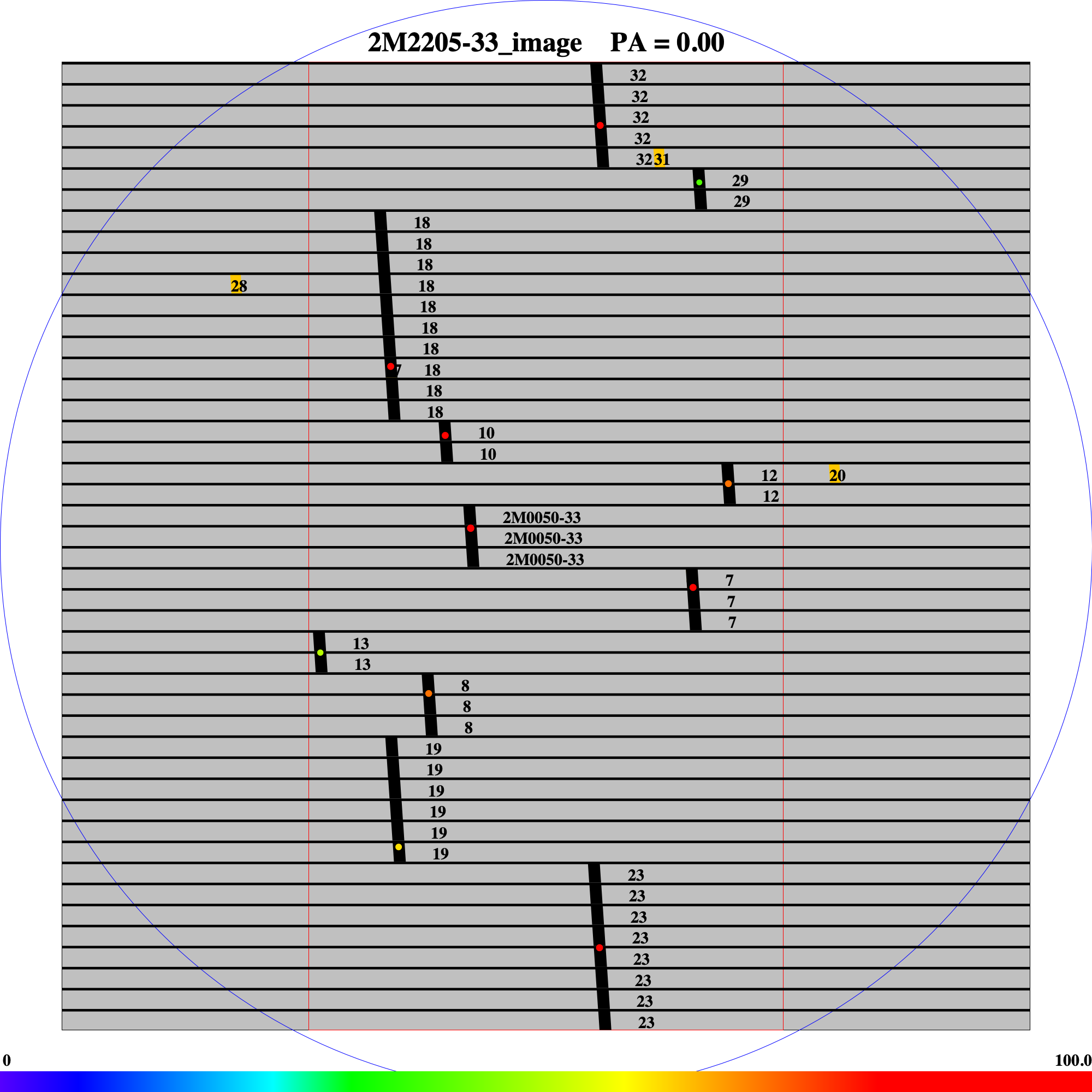
Near-infrared multiobject spectrographs like MOSFIRE (McLean et al., 2010, 2012) installed at the Keck I telescope, allow us to perform spectro-photometric monitoring of brown dwarfs from the ground. As explained in Manjavacas et al. (2021), to carry out spectro-photometric monitoring observations of brown dwarfs from the ground, we need calibration stars in the same field of our targets to account for spectral calibration, telluric contamination, changes in the airmass, humidity and temperature variations in the atmosphere, etc, that might potentially introduce spurious variability signals. MOSFIRE performs simultaneous spectroscopy of up to 46 objects in a 6.1’x 6.1’ field of view, using the Configurable Slit Unit (CSU), a cryogenic robotic slit mask system that is reconfigurable electronically in less than 5 minutes without any thermal cycling of the instrument. A single photometric band is covered in each instrument setting ($Y$, $J$, $H$ or $K$).

The total time of $J$- and $H$-band monitoring is $\sim$2.67 hr, with a gap of $\sim$25 min between the $J$-band imaging and spectroscopic data. We observed $\sim$0.45 hr in $J$-imaging mode, $\sim$0.35 hr in $J$-band spectrophotometric mode, and 1.36 hr in $H$-band spectrophotometric mode

We observed 2M0050–3322 on UT 2020-10-09 during $\sim$2.6 hr, covering approximately two rotational periods of the object. Since the target has a high proper motion, we designed the MOSFIRE mask accordingly with the predicted position of the target at the time of the observation. Nonetheless, we did not find our target in the slit as expected. Thus, we performed $J$-band imaging of the field during the first $\sim$0.45 hr of the observation, while we designed a new mask, after having identified our target in the imaging data. We took images of the 6.1’$\times$6.1’ field of view, with a scale of 0.1798”/pix, performing a 3.0” ABBA pattern. We integrated during 11 s in each ABBA position. After designing a new mask, we interrupted the observations for $\sim$25 min between the $J$-band imaging and spectroscopic data while installing the new MOSFIRE mask. Then, we obtained $J$-band spectra of 2M0050–3322 for $\sim$0.35 hr, covering the first rotational period of the target. We obtained three spectra of 2M0050–3322 in the $J$-band (1.153–1.352 $\mu$m) using a 1.5” ABBA pattern. As in Manjavacas et al. (2021), we used wide slits of 4.5” to avoid slit losses for all calibration stars and the target, obtaining a spectral resolution of R$\sim$1000. Immediately, we obtained another nine spectra in the $H$-band (1.5280-1.8090 $\mu$m) during $\sim$1.4 hr, covering the second rotational period of 2M0050–3322. In Table 1 we show the list of objects used as calibrators, their coordinates, and their $J$-band magnitudes. Those that do not have an object number did not have sufficient signal-to-noise (SNR) to be used as calibrator stars (SNR $<$ 5). In Figure 1, we show the configuration of the CSU mask, with the position of the target and the calibration stars. We used exposure times of 120 s for each ABBA nod position in the the first ABBA. We observed over an airmass range 1.79 to 2.37.

For data reduction purposes, 11 dome flats of 2 s exposure were obtained in the $J$- and $H$-band. Following the same calibration strategy as in Manjavacas et al. (2021), we obtained three $J$- and $H$-band ”sky” spectra using the same configuration for the multiobject mask as for the observations, but using 1.0” slits to obtain higher resolution sky lines during 1 s. The 1.0” slits provided spectra of the skylines with enough resolution to allow the pipeline to produce an accurate wavelength calibration. We used archive imaging flats and darks taken on 2020-09-04.

Table 1: Information about the calibration objects in the field of 2M20050–3322.

Num. mask	Num. obj.	RA (J2000)	DEC (J2000)	$J$-mag
32	5	00:50:17.976	-33:19:49.25	15.64
29	–	00:50:14.982	-33:20:10.84	18.58
18	–	00:50:24.317	-33:21:20.61	17.48
10	3	00:50:22.666	-33:21:46.78	16.15
12	6	00:50:14.095	-33:22:05.07	16.56
2M0050-33	2M0050-33	00:50:21.900	-33:22:21.95	15.93
7	–	00:50:15.175	-33:22:44.41	17.74
13	–	00:50:26.454	-33:23:09.12	19.54
8	–	00:50:23.165	-33:23:24.61	18.23
19	2	00:50:24.075	-33:24:22.80	14.93
23	1	00:50:17.997	-33:25:01.00	15.85

Figure 1: Illustration of the positioning of the CSU bars (black horizontal lines) on MOSFIRE to obtain simultaneous multi-object spectroscopy of the field of 2M0050–3322 as produced by MAGMA, the MOSFIRE Automatic GUI-based Mask Application. Our target (named as 2M0050-33) is placed in the center of the field. The position of the comparison stars as shown in Table 1 are also marked. The round colored points show the expected positions of the target and calibration stars. The different colors indicate the weight given to each object for MAGMA to prioritize the desired objects in the field of view. As shown in the color-bar, red is weight 100 and blue weight 0. The yellow squares show the position of the stars used for the alignment of the mask. The blue circle indicates the field of MOSFIRE. The vertical red lines delimits the area in which the slits are positioned for spectroscopy in any filter.

4 Data Reduction

4.1 Imaging data

We reduced the $J$-band imaging data independently from the spectroscopic data. All $J$-band raw images were dark subtracted using a median-combined dark. Then we divided them by a median-combined flat field, created using the median-combined and subtracted lamp-on and lamp-off flats. We created a bad-pixel mask to mask hot and dead pixels. We flagged those pixels by selecting the pixels in the master flat calibration image with values 2$\sigma$ above or below the mean. We subtracted the A-B pairs and the B-A pairs independently to remove the sky. Finally, the A-B and B-A pairs were aligned and coadded.

To perform the aperture photometry on the reduced imaging data, we used the Python package DAOStarFinder from astropy.photutils, an implementation of the daofind algorithm (Stetson, 1987), that searches images for local density maximum that have a peak amplitude greater than a specified threshold (the threshold is applied to a convolved image) and have a size and shape similar to a defined 2D Gaussian kernel. Then, we performed aperture photometry using the Python package aperture_photometry from astropy.photutils with an aperture of 5 pixels, in an annulus between 6 and 10 pixels to extract the background. Finally, using the x and y position of the stars, we matched the photometry of all stars in all the $J$-band images to obtain a light curve for each individual star.

4.2 Spectroscopic data

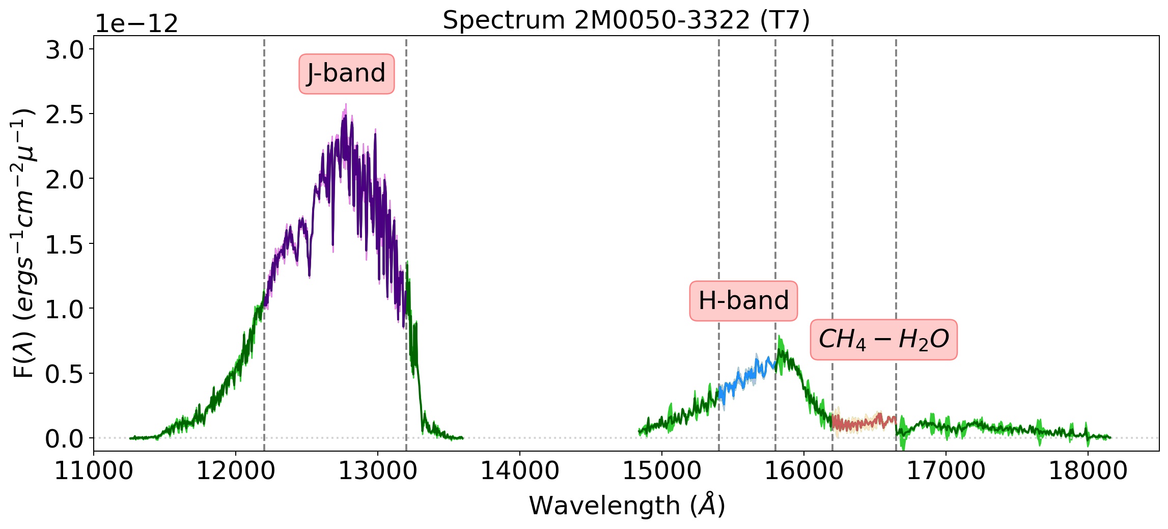
We used the version 1.7.1 of PypeIt to reduce the multi-object spectro-photometric data acquired with MOSFIRE in the $J$- and $H$-band (Prochaska et al., 2019, 2020). The pipeline corrected the raw images from dark current, and a bad pixels mask is generated. The edges of the slits were traced using the dome flats, and a master flat was also created. PypeIt produced a wavelength calibration for our data using the sky arc frames taken using the same multiobject mask we employed for our observations, but with narrower slits of 1.0”. The wavelength calibration accounted for the spectral tilt across the slit. The calibrations were applied to our science frames, and the sky was subtracted using the A-B or B-A frames following Kelson (2003). The 1D science spectra were extracted from the 2D sky-corrected frames. The signal-to-noise achieved for the target and the calibration stars in the $J$-band and $H$-band spectro-photometric data are summarized in Table 2. No telluric calibration was performed for these spectra. Instead, for the upcoming analysis, we have used the wavelength range between 12200 and 13200 $\AA$, avoiding the most prominent telluric contamination in the $J$-band, and the range between 15400 and 15800 $\AA$ for the $H$-band. We show the median-combined, flux-calibrated $J$- and $H$-band MOSFIRE spectrum in Fig. 2. The flux calibration was performed using the 2MASS $J$- and $H$-band magnitudes. We convolved our near-infrared spectra with $J$-, and $H$- filter transmission curves of 2MASS. The resulting spectra were integrated. We calculated the flux for our targets corresponding to the $J$, and $H$ bands using 2MASS magnitudes. Finally, we calculated the scaling factor for the J, and H bands and multiplied our near-infrared spectra in J, and H filters to have the same flux as given by 2MASS.

Table 2: Median signal-to-noise of the $J$-band and $H$-band spectra of the target and the calibration stars.

Object Number	$J$-band SNR	$H$-band SNR
Star 1	15.4	13.1
Star 2	30.6	29.4
Star 3	13.0	10.5
Star 5	16.6	13.4
2M0050–3322	52.9	27.7

Figure 2: Median-combined, flux-calibrated $J$- and $H$-band MOSFIRE spectrum of 2M0050–3322, and its uncertainties in lighter colors. We mark in violet the wavelength range used to obtain the $J$-band spectroscopic light curve, in blue the $H$-band spectroscopic light curve, and in orange the $\mathrm{CH_{4}-H_{2}O}$ light curve.

5 Light curve correction

For the spectro-photometric data, we produced a $J$-band (12200 and 13200 $\AA$), a $H$-band (15400 and 15800 $\AA$), and a $CH_{4}-H_{2}O$ (16200-16650 $\AA$) light curve for each object in the field. As these data were obtained from the ground, there might be other additional sources of non-astrophysical contamination affecting the shape of the light curve extracted for each object, such as varying atmospheric transparency, change in the water vapor content of the atmosphere, the seeing, variations in the outside temperature during the observation, wind speed and direction variations, airmass variations, etc. Thus, the science target light curve needs to be corrected for these potential sources of contamination. We corrected all the light curves of the target using the same wavelength range of the calibration stars spectra. Using this method, we expect to correct most of the spurious variability signal introduced by telluric contamination.

To perform the light curve correction of the photometric and spectro-photometric datasets, we followed a similar approach to Radigan et al. (2014). Each light curve was corrected by dividing it by a calibration light curve produced by median combining the relative-flux light curves of all the other objects in the field, beside the science target. First, we normalized the light curves of all objects to the median flux of each of them. For each reference star, a calibration light curve was created by median combining the light curves of all the other objects, beside the science target. Then, the raw light curve of each calibration star was divided by its corresponding calibration light curve to obtain a corrected light curve. Finally, we measured the standard deviation, $\sigma$, of the corrected light curve of each calibration star.

To perform an optimal correction of the 2M0050–3322 light curve we chose the least intrinsically variable calibration stars. We followed the best-selection criteria for the calibration stars used by Radigan et al. (2014), for which they subtracted from the corrected light curve of each calibration star, a shifted version of itself, and divided it by $\sqrt{2}$ ($\sigma_{s}=[f_{cal}-f_{cal\_shifted}]/\sqrt{2}$). Radigan et al. (2014) then identified poor-quality calibration stars as those where $\sigma_{s}>1.5\times\sigma_{target}$, but in our case d. These criteria left only 5 stars as good calibrators for the $J$-band imaging data, and only stars 1 and 2 as valid correcting stars in the $J$-band spectroscopic data. For the $H$-band spectro-photometric light curve only star 6 was rejected. For the $CH_{4}-H_{2}O$ light curve no stars were rejected following Radigan et al. (2014) method, but stars 3, 5 and 6 did not improve their standard deviation after correcting them, so we decided to leave the, out as calibration stars (see Table 6). In Tables 3, 4, 5, 6, and 7, we show the standard deviation of all the calibration stars and 2M0050–3322 before and after correcting each light curve. In the case of the spectrophotometric $J$-band light curves the $\sigma$ improves only marginally, probably due to the few points of the light curve.

Table 3: Standard deviation of the $J$-imaging photometric light curve for the ”good” calibration stars.

(x centroid, y centroid)	$\sigma$ non-corrected LC	$\sigma$ corrected LC
(1158.94, 202.79)	0.0180	0.0055
(212.59, 836.39)	0.0150	0.0047
(1423.89, 1181.28)	0.0136	0.0055
(829.97, 1280.67)	0.0146	0.0042
(1151.96, 1931.35)	0.088	0.0084

Table 4: Standard deviation of the $J$-band spectro-photometric light curve for the calibration stars.

Object Number	$\sigma$ non-corrected LC	$\sigma$ corrected LC
Star 1	0.0021	0.0023
Star 2	0.0019	0.0017

Table 5: Standard deviation of the $H$-band spectro-photometric light curve for the calibration stars.

Object Number	$\sigma$ non-corrected LC	$\sigma$ corrected LC
Star 1	0.0077	0.0075
Star 2	0.0083	0.0018
Star 3	0.0066	0.0056
Star 5	0.0084	0.0022

Table 6: Standard deviation of the $\mathrm{CH_{4}-H_{2}O}$-band spectro-photometric light curve for the calibration stars.

Object Number	$\sigma$ non-corrected LC	$\sigma$ corrected LC
Star 1	0.0102	0.0056
Star 2	0.0058	0.0038

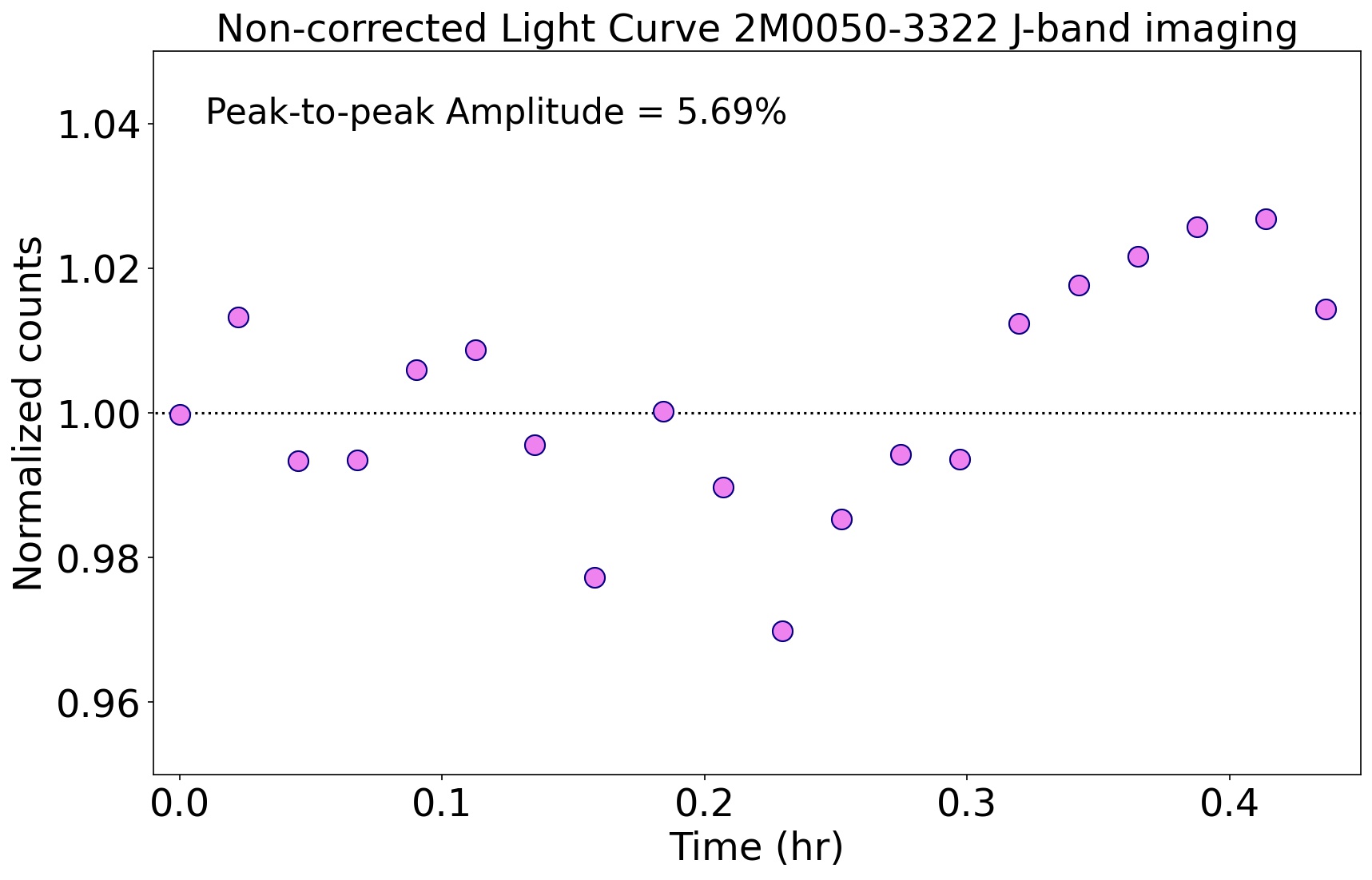
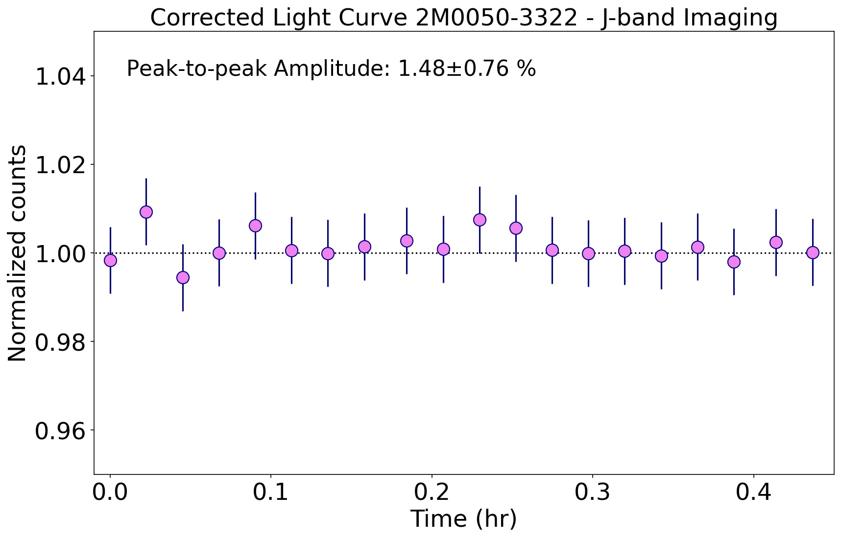
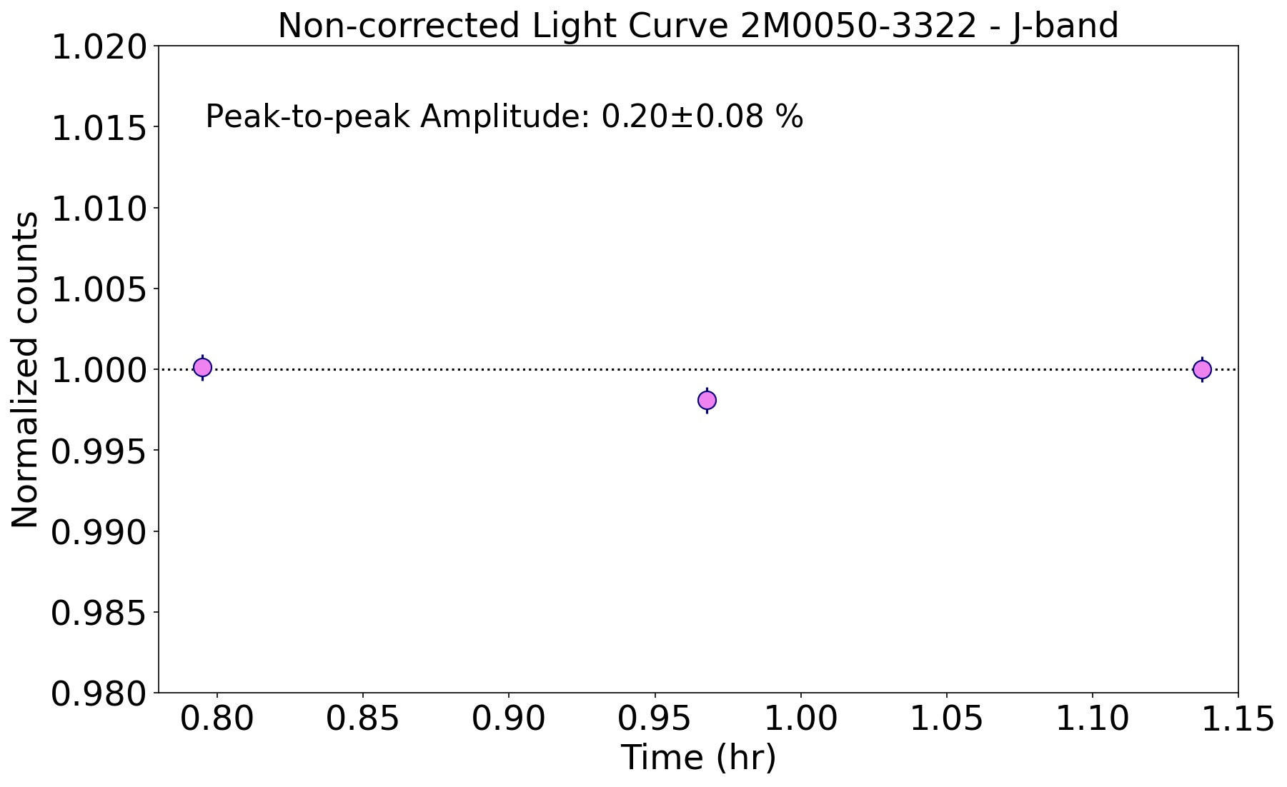
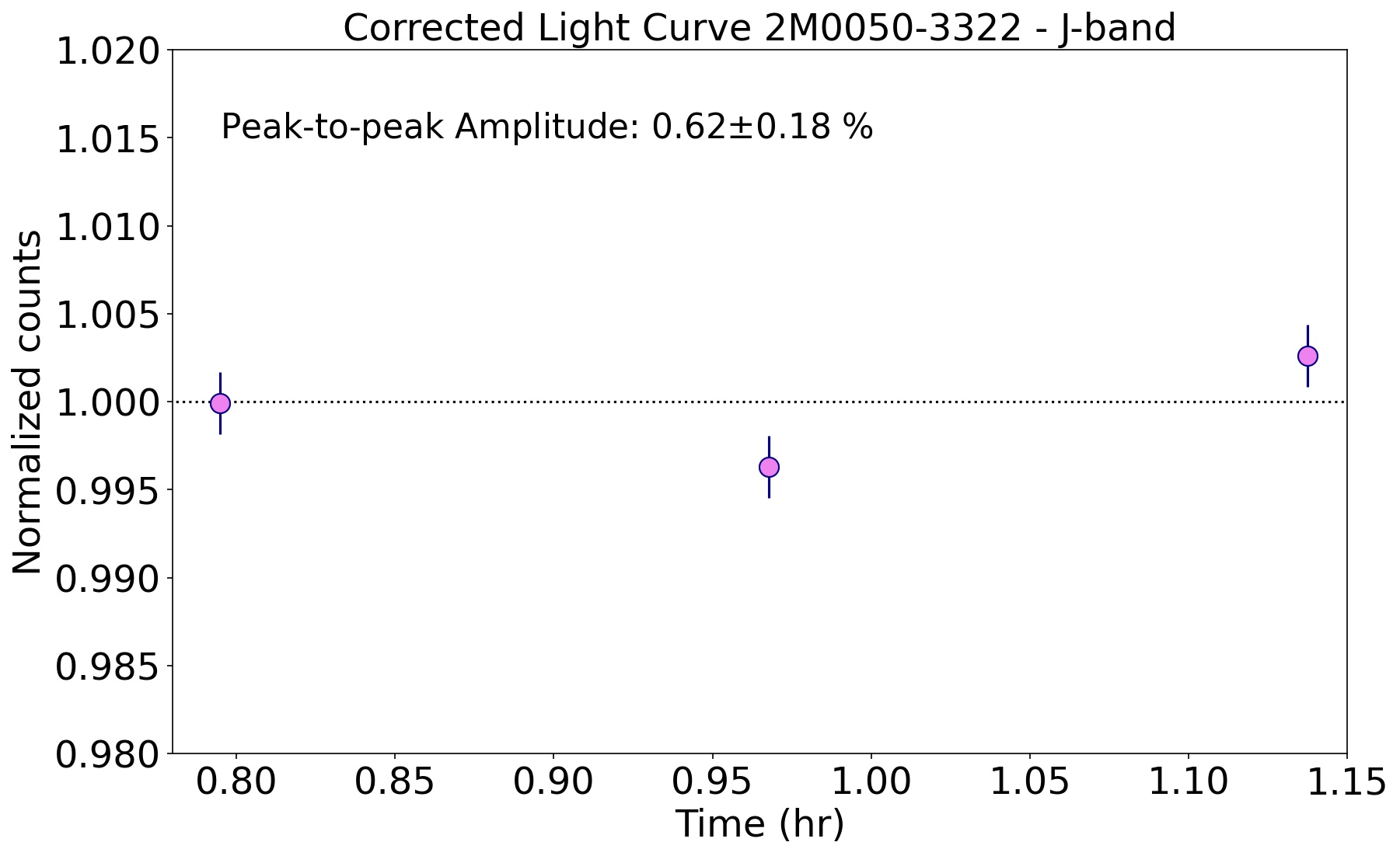
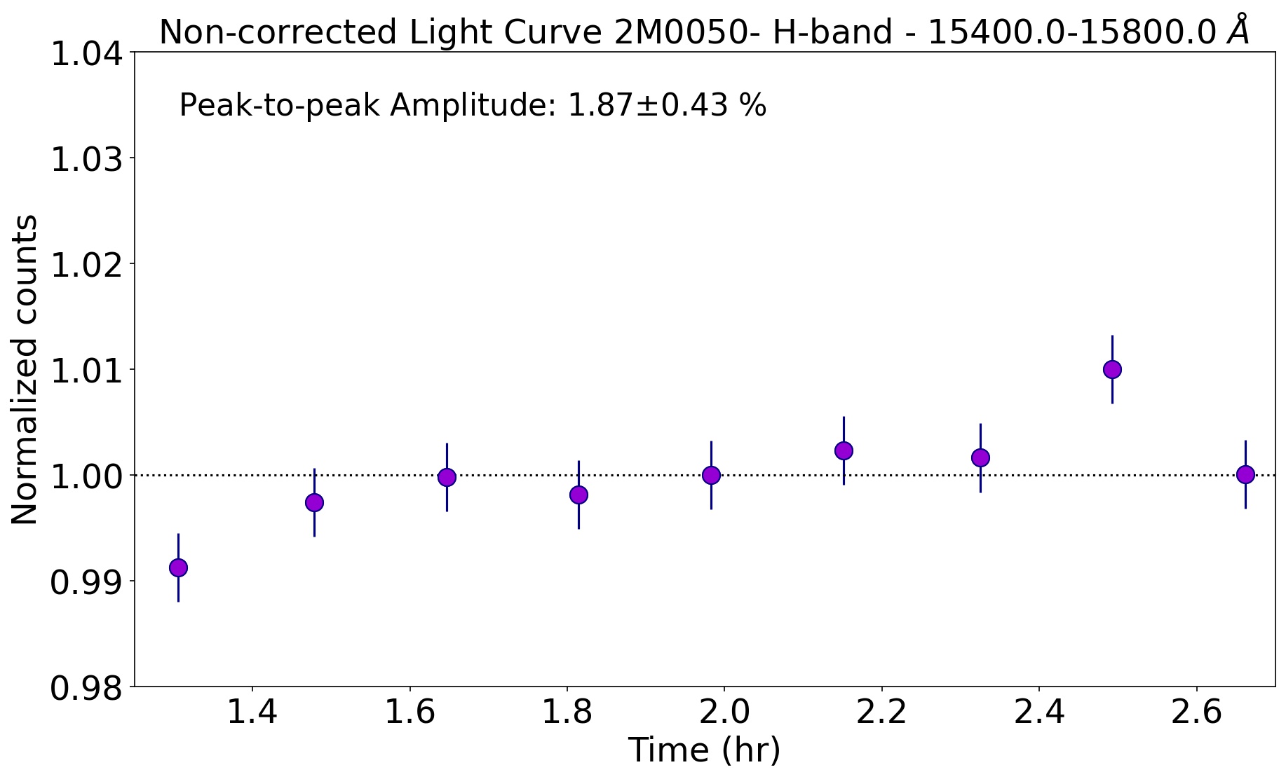
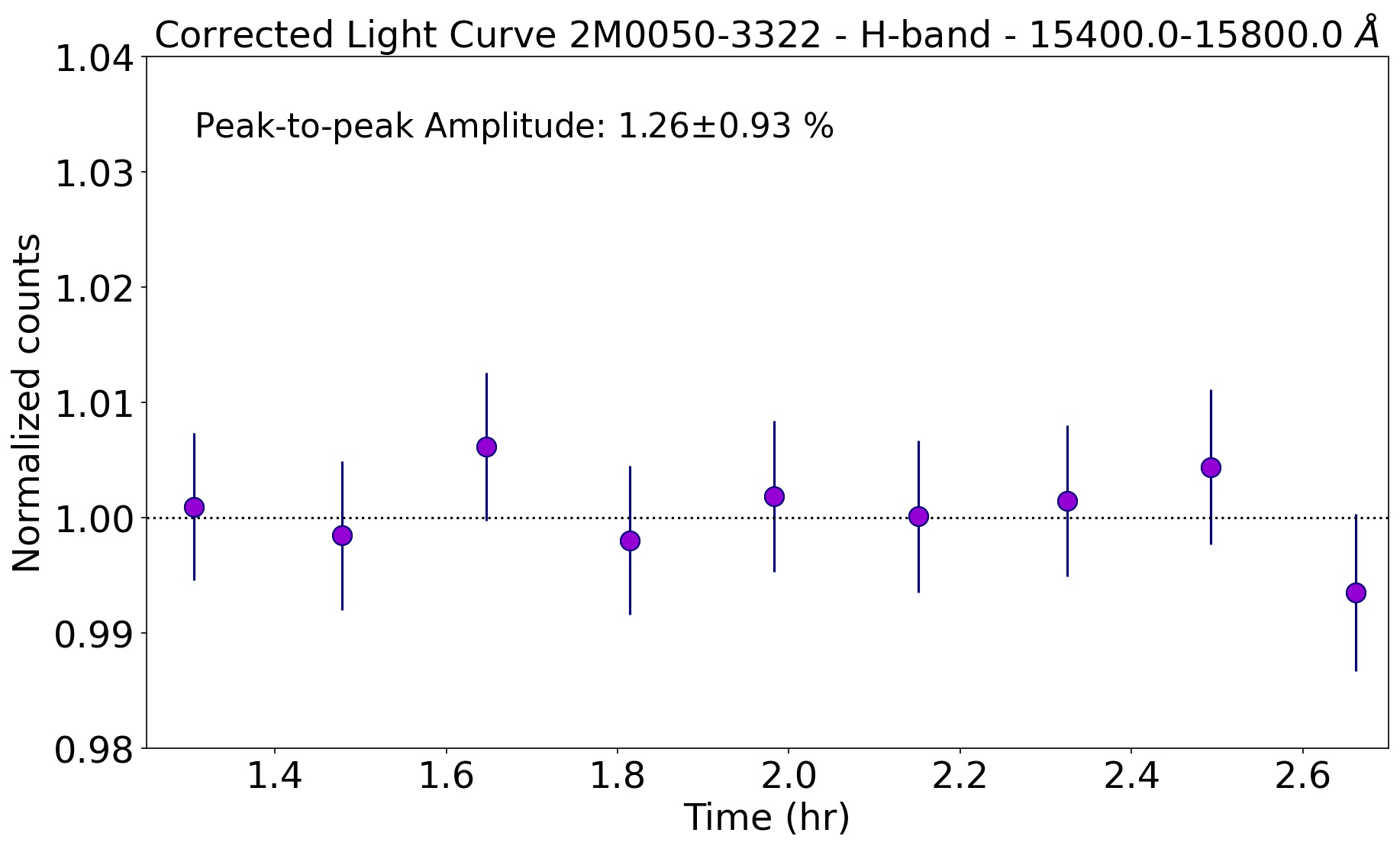
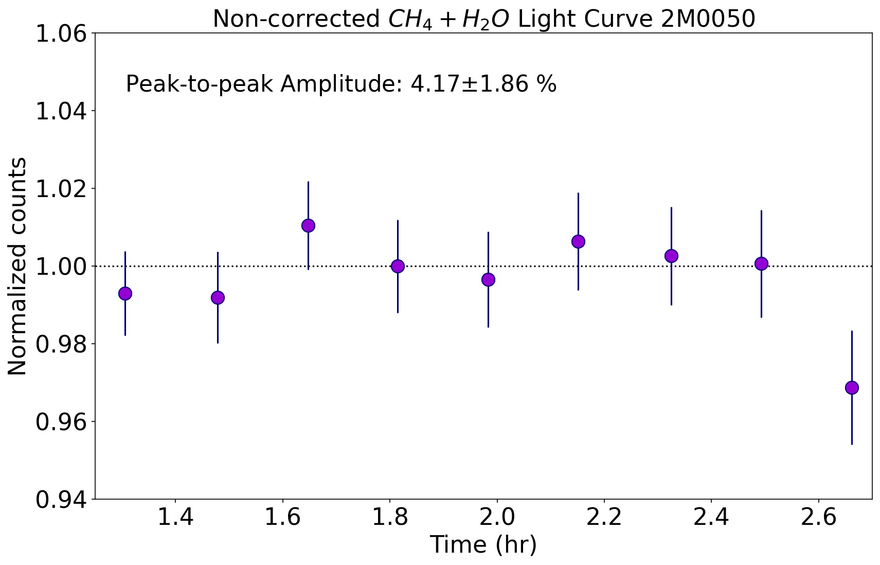
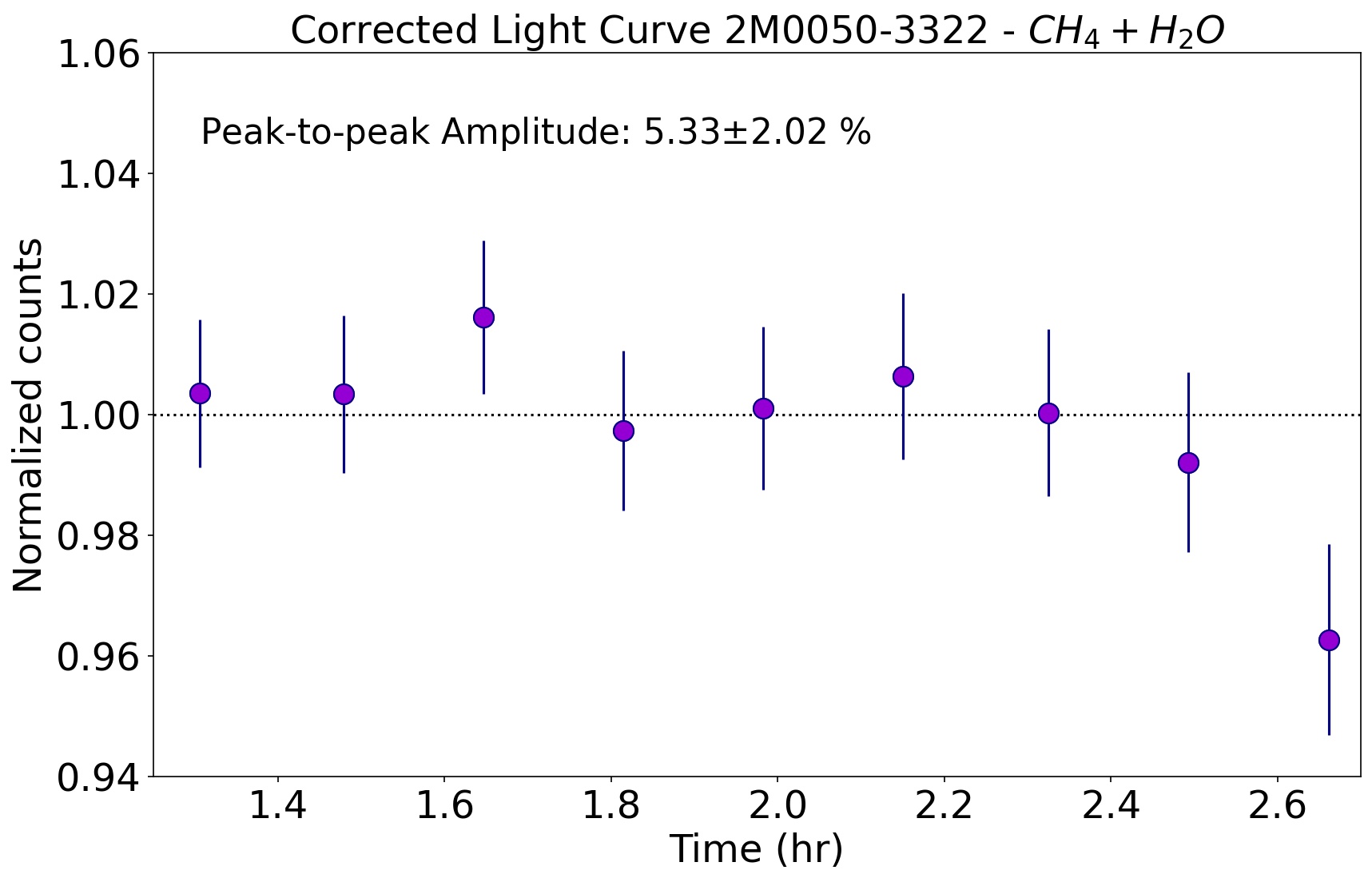
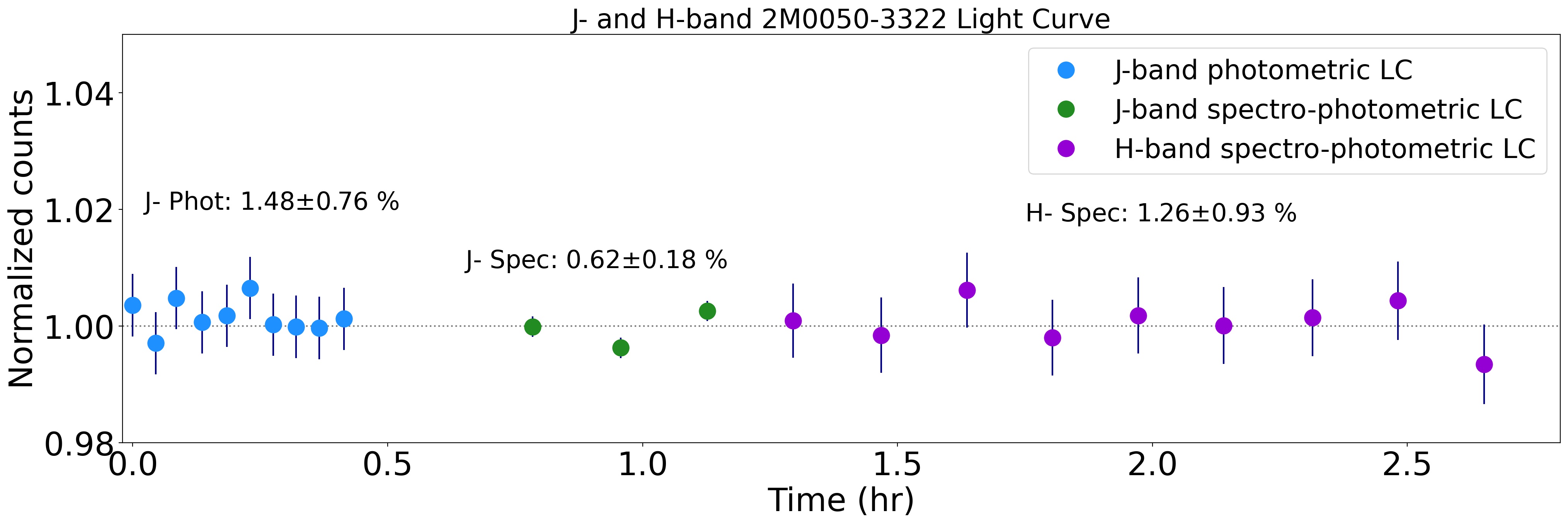
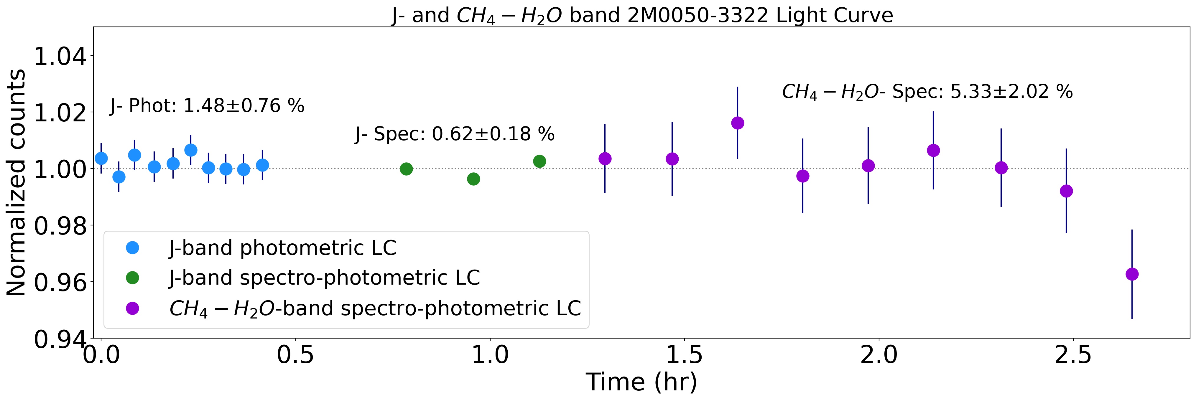
As in Manjavacas et al. (2021), PypeIt’s formal instrumental uncertainties underestimate the uncertainties of 2M0050–3322 light curve, since it does not necessarily account for spurious variability introduced by changes in the Earth’s atmosphere during the observation. Thus, as we did in Manjavacas et al. (2021), we added the mean of the $\sigma_{s}$ calculated for the target and the selected calibration stars as the uncertainty for each point in the light curve of the target (0.0057). The non-corrected light curves of 2M0050–3322 are shown in Fig. 3, 4, 5, 6 left, and the corrected light curves in Fig. 3, 4, 5 and 6 right. All corrected and normalized light curves are shown together in Fig. 7. In this figure every two data points of the original $J$-band imaging light curve in Fig. 3 were combined for clarity.

Figure 3: Normalized non-corrected (left) and corrected (right) $J$-band imaging light curves of 2M0050–3322. We indicate the peak-to-peak amplitudes of their fluctuations.

Figure 4: Normalized non-corrected (left) and corrected (right) $J$-band light curves of 2M0050–3322. We indicate the peak-to-peak amplitudes of their fluctuations.

Figure 5: Normalized non-corrected (left) and corrected (right) $H$-band light curves of 2M0050–3322. We indicate the peak-to-peak amplitudes of their fluctuations.

Figure 6: Normalized non-corrected (left) and corrected (right) $CH_{4}-H_{2}O$-band light curves of 2M0050–3322. We indicate the peak-to-peak amplitudes of their fluctuations.

Figure 7: Corrected $J$-imaging, $J$-band, $H$-band and $\mathrm{CH_{4}-H_{2}O}$ light curves of 2M0050–3322, and the peak-to-peak amplitudes of their fluctuations.

Table 7: Statistics of the $J$-band imaging, $J$- and $H$-band spectro-photometric light curves of 2M0050–3322, and the peak-to-peak amplitudes of their fluctuations.

Light curve (LC)	$\sigma$ non-corrected LC	$\sigma$ corrected LC	Peak-to-peak non-corrected LC	Peak-to-peak corrected LC
$J$–imaging	0.0153	0.0034	$\sim$5.69 %	1.48$\pm$0.75 %
$J$–spec	0.0002	0.0039	0.20$\pm$0.08 %	0.62$\pm$0.18 %
$H$–spec	0.0027	0.0036	1.87$\pm$0.43 %	1.26$\pm$0.93 %
$\mathrm{CH_{4}-H_{2}O}$–spec	0.0095	0.0024	4.17$\pm$1.86 %	5.33$\pm$2.02 %

6 Correlation Analysis

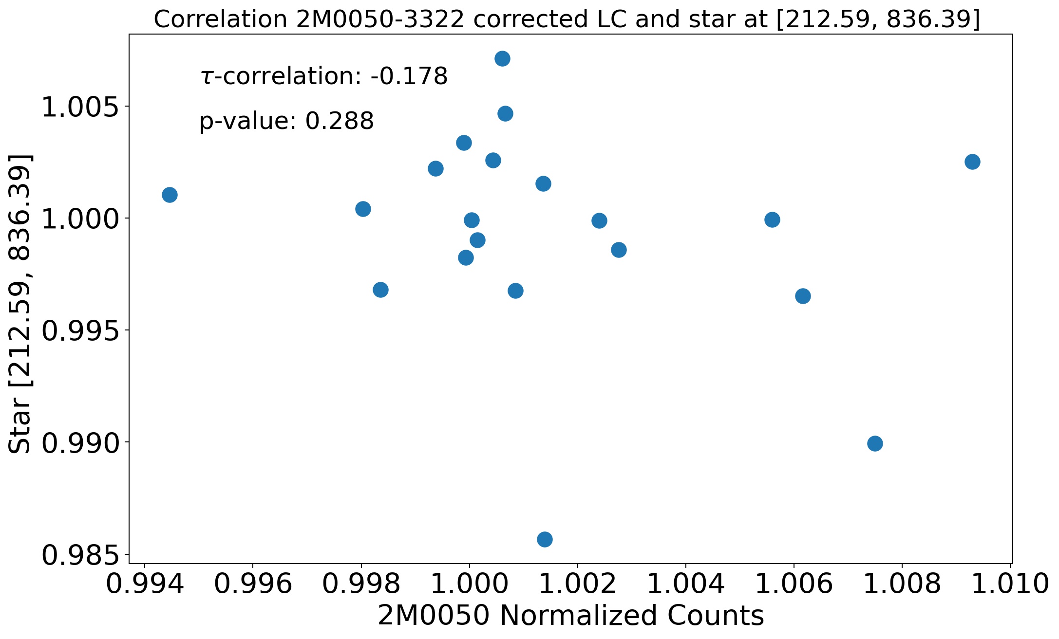
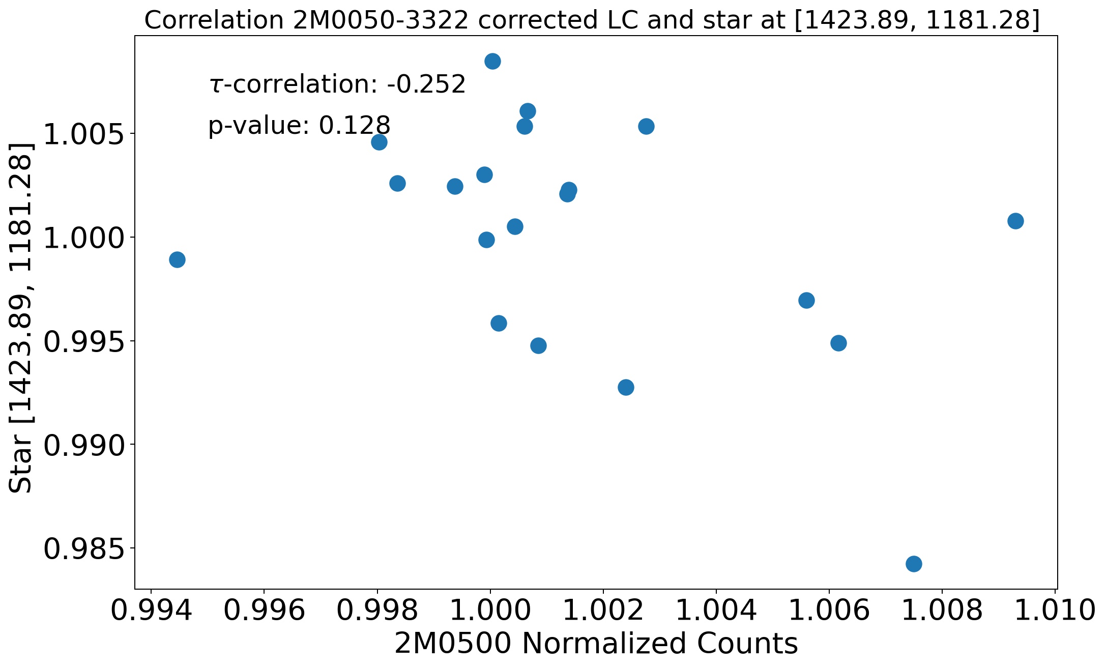
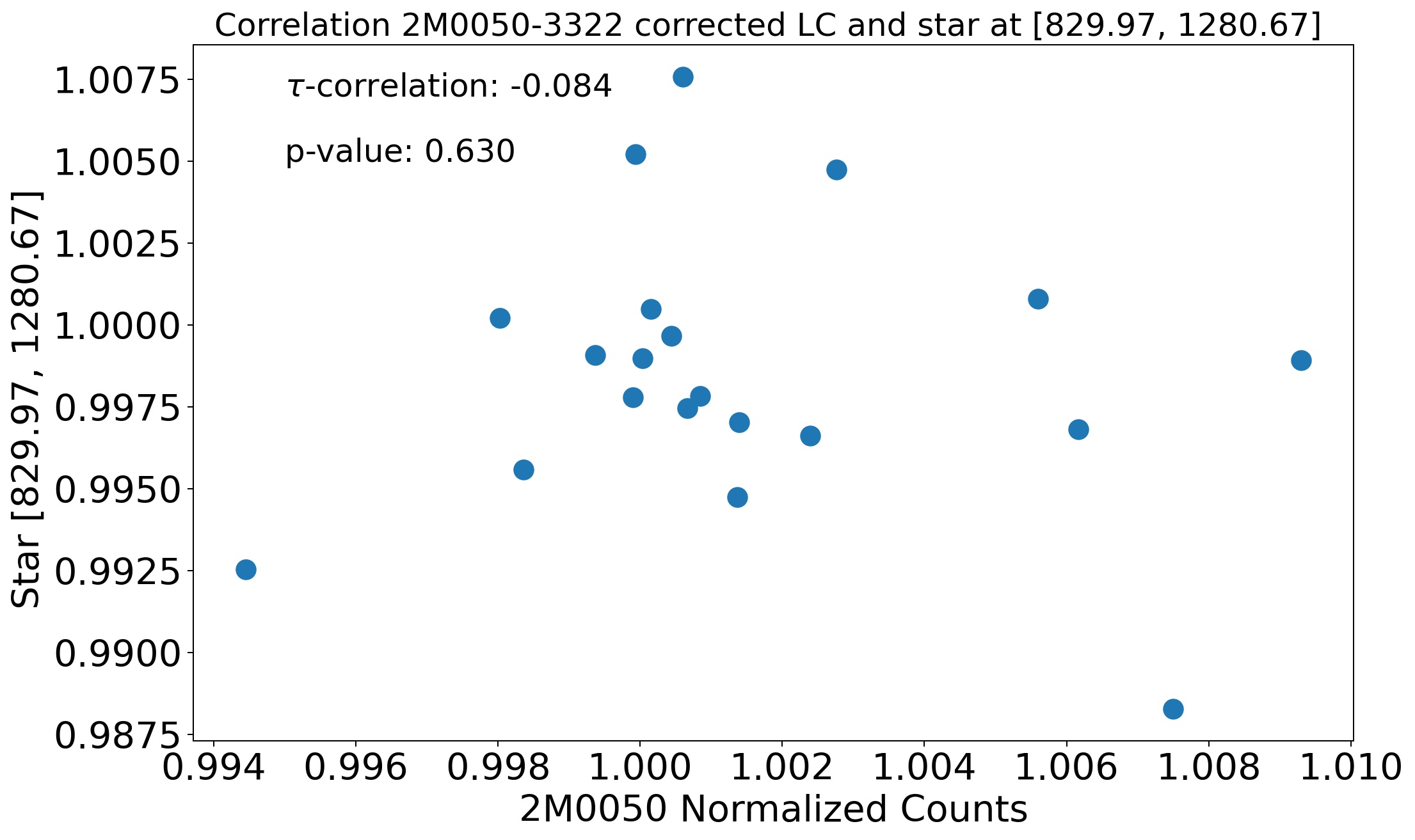
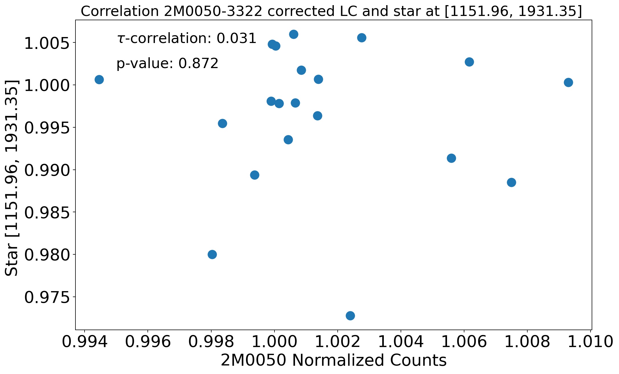
In this section, we analyze the different sources of external spurious contamination in the $J$-imaging, $J$-band spectrophotometric data, the $H$-band spectrophotometric, and the $\mathrm{CH_{4}-H_{2}O}$ data that could potentially lead to non-astrophysical, spurious variability introduced in the 2M0050–3322 light curves. We measure the Kendall $\tau$ correlation between different parameters, since it is a more robust correlation estimator than other estimators (Croux & Dehon, 2010). In addition, we provide the significance (p-value) of each correlation, where numbers close to 0.0 suggest that the correlation obtained is significant. We consider that there is no correlation for Kendall $\tau$ values close to 0.0, a weak correlation for absolute Kendall $\tau$ values between 0.1 and 0.4, a moderate correlation for values between 0.4 and 0.7, and a strong correlation for values above 0.7.

6.1 Comparison between Stars and Target Light Curves

To evaluate the effects of potential contamination on the target’s light curve due to the Earth’s atmosphere, we investigate the correlation between the non-corrected and corrected light curves of the target, and the comparison stars in the $J$- and $H$-band.

6.1.1 $J$-band data

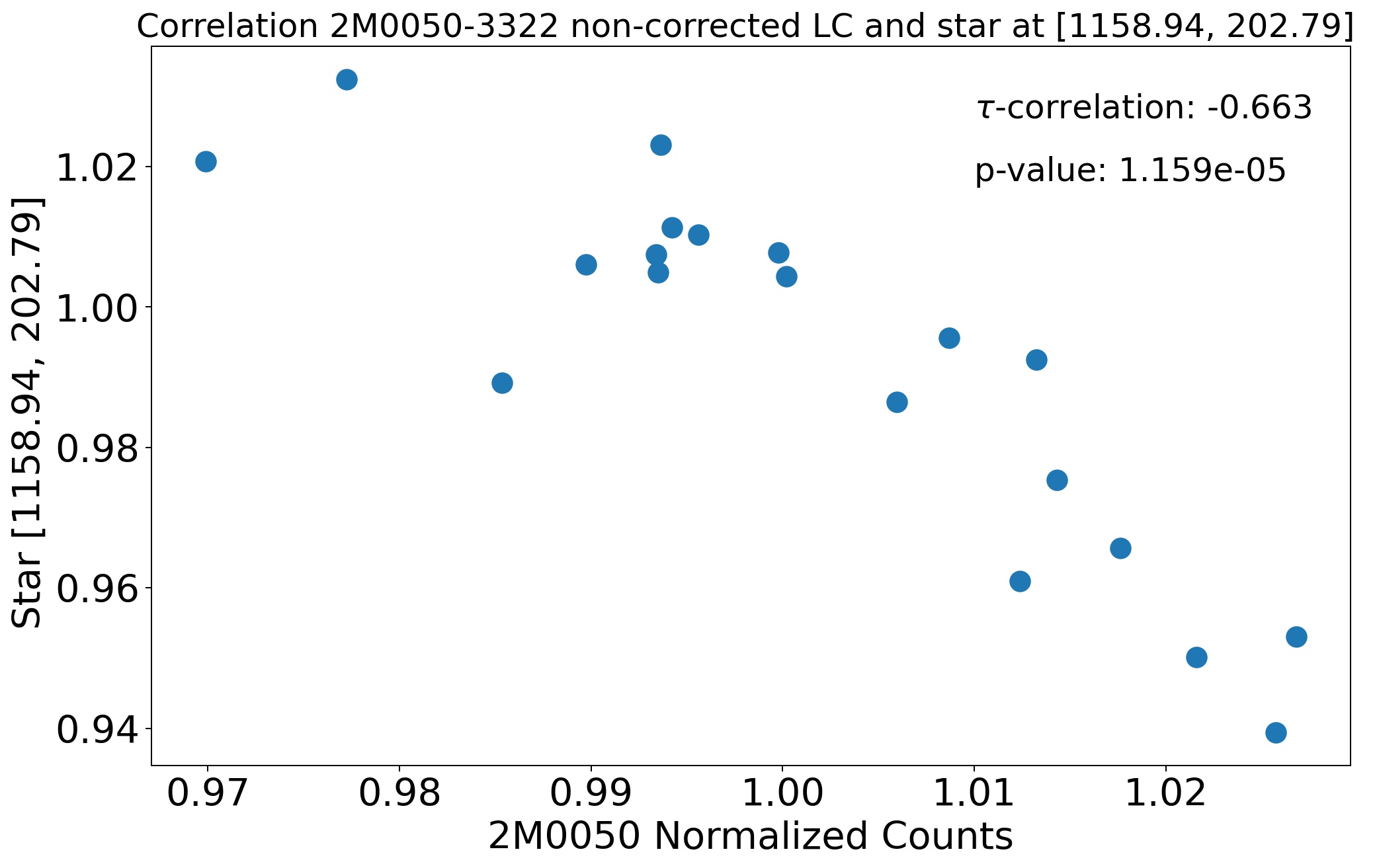
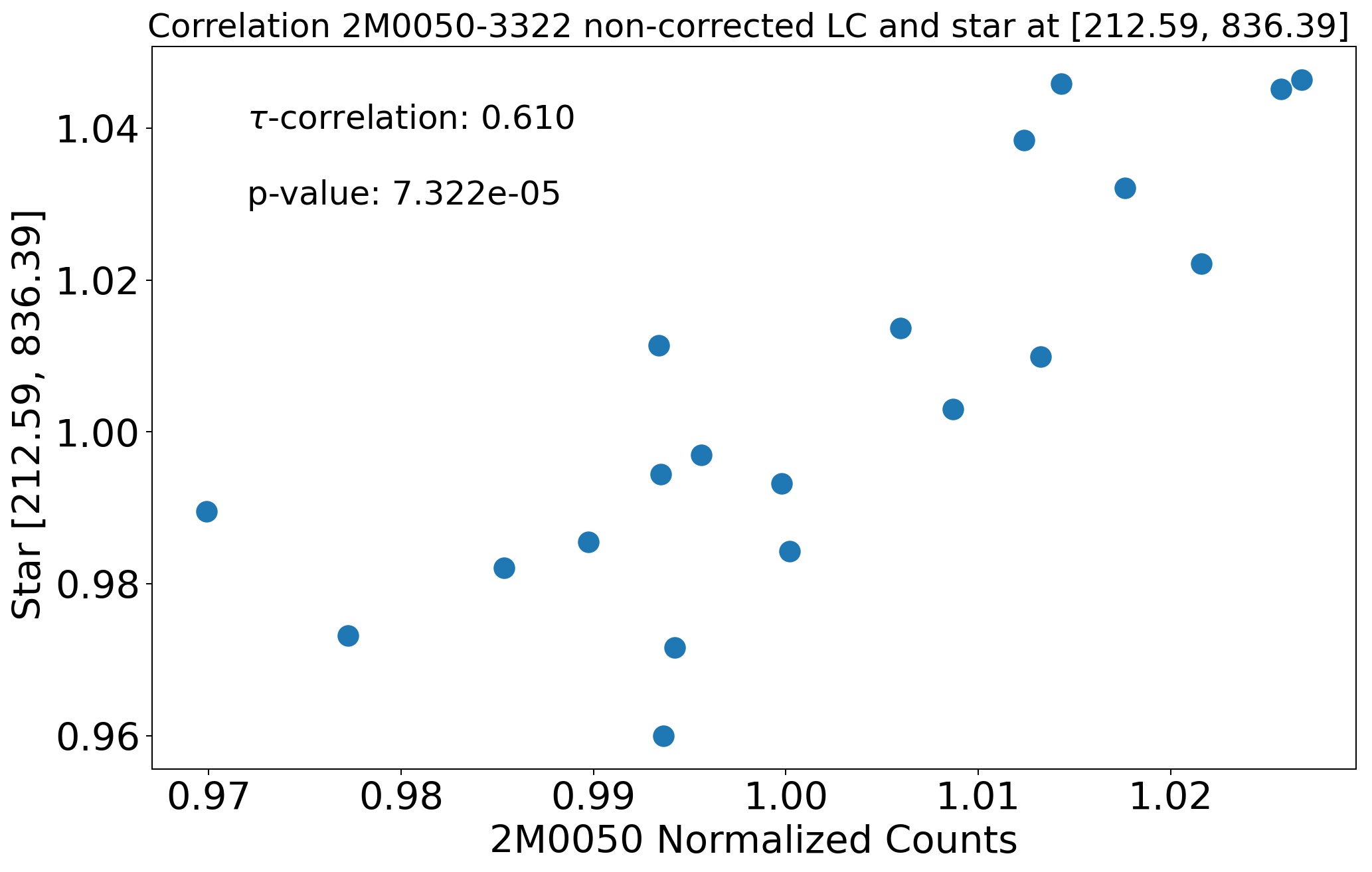
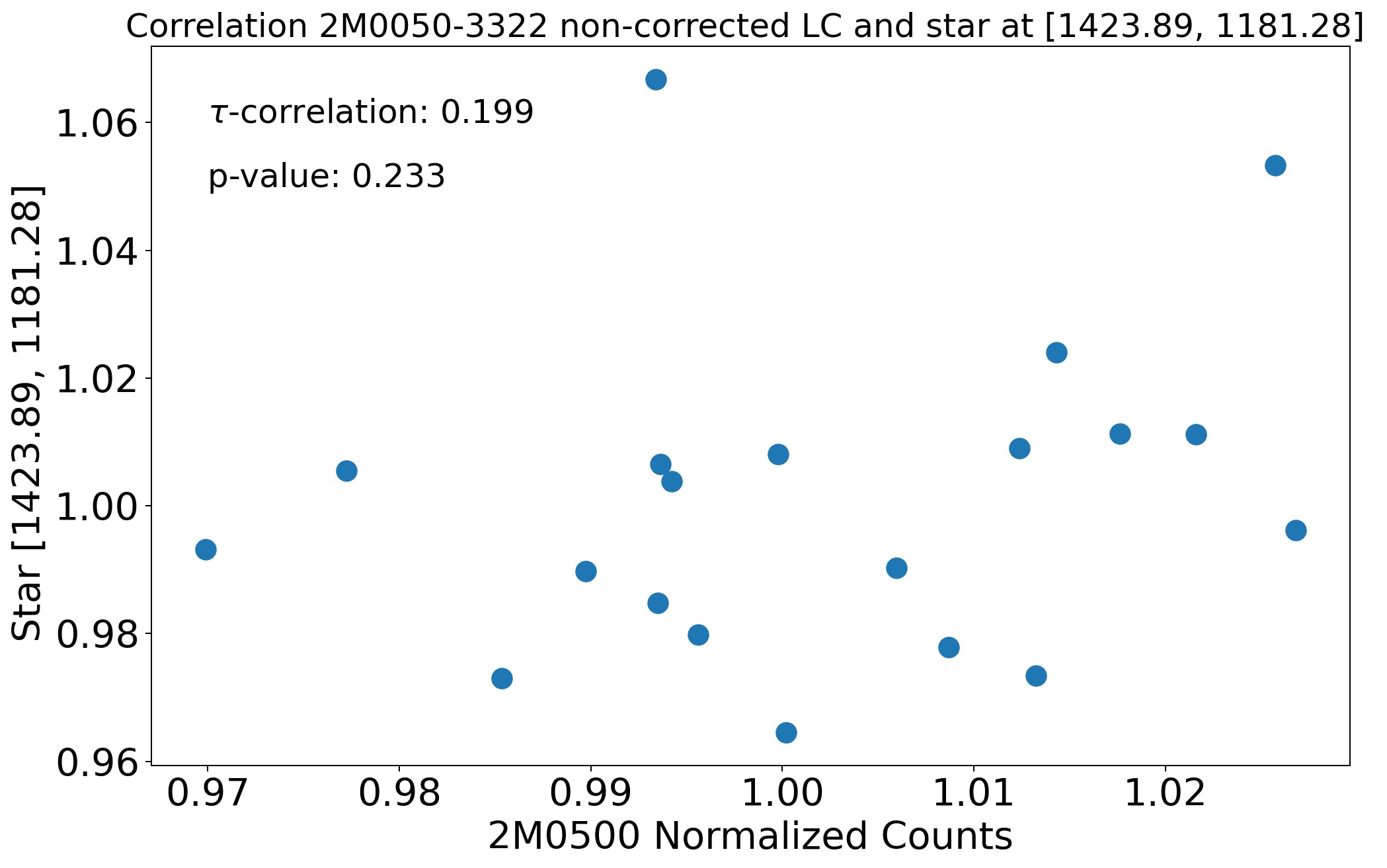
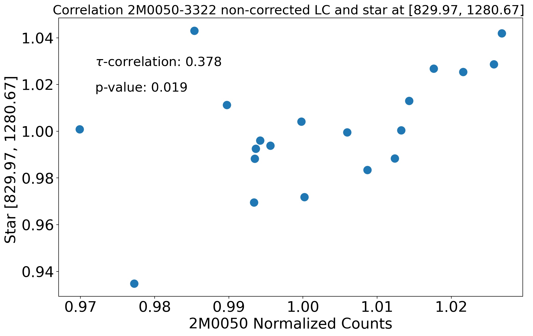
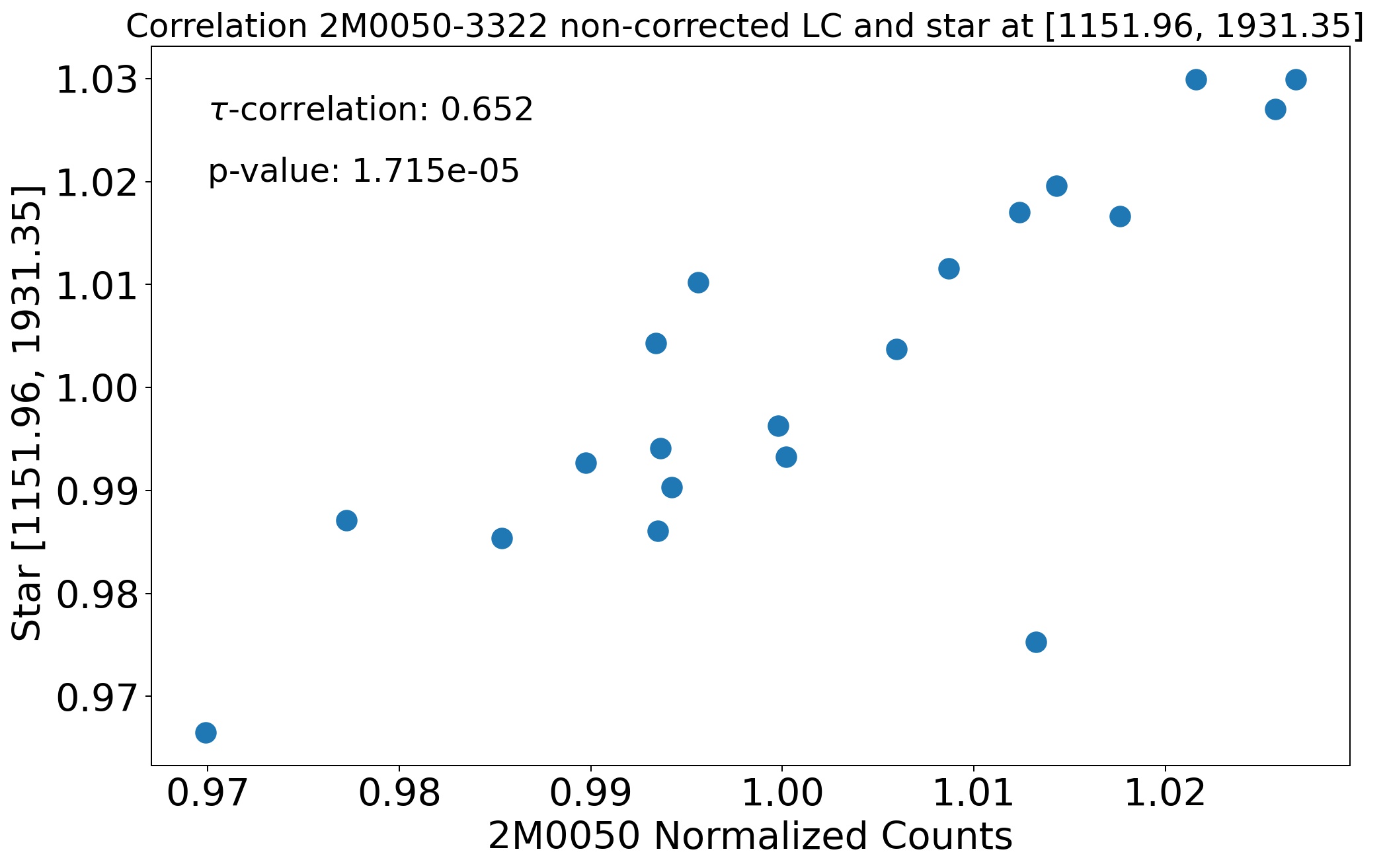
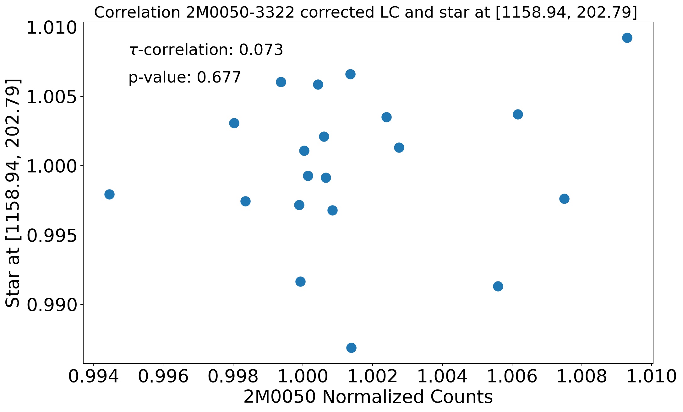
We calculate the Kendall’s $\tau$ coefficients to estimate the correlation between the target’s $J$-band imaging data and the ”good” calibration stars’ light curves. We find weak to moderate correlation for some calibration stars, with correlations varying from -0.66 (p-value = 1.15e-05), to 0.65 (p-value = 1.75e-05). When we correct the calibration stars’ and the target’s light curves, we remove also most of the correlations between them, obtaining Kendall’s $\tau$ coefficients between 0.07 (p-value = 0.67), and -0.34 (p-value = 0.03). In Fig. 16 and 17 of the Appendix we show the correlations of the ”good” calibration stars light curves before and after correction.

We do not calculate these correlations for the $J$-band spectrophotometric data, since we have only three data points, which would not provide meaningful correlations.

6.1.2 $H$-band data

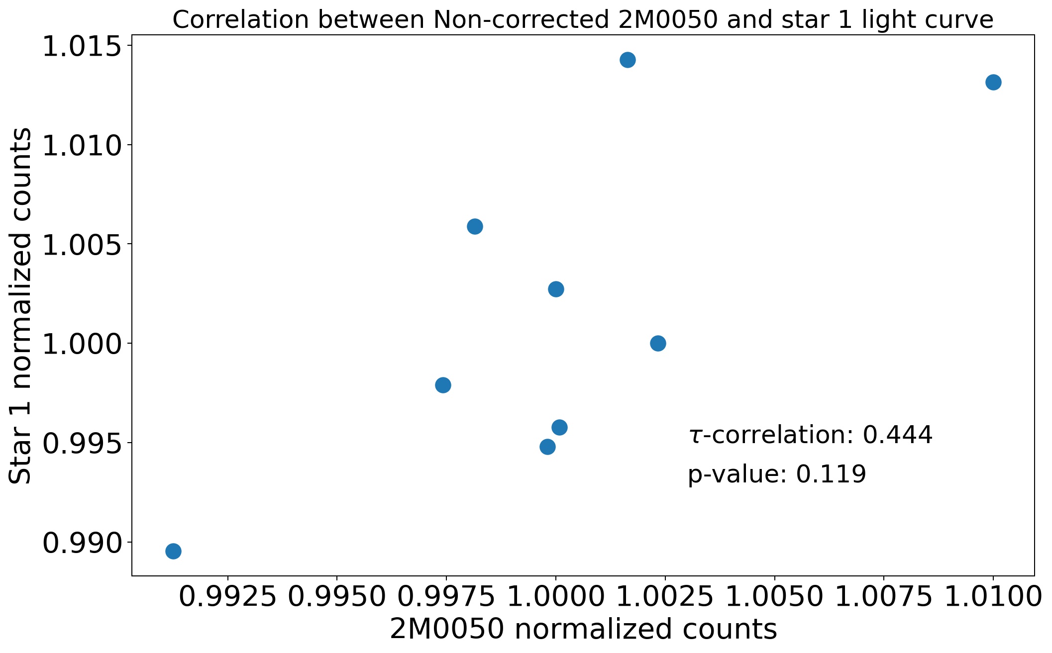
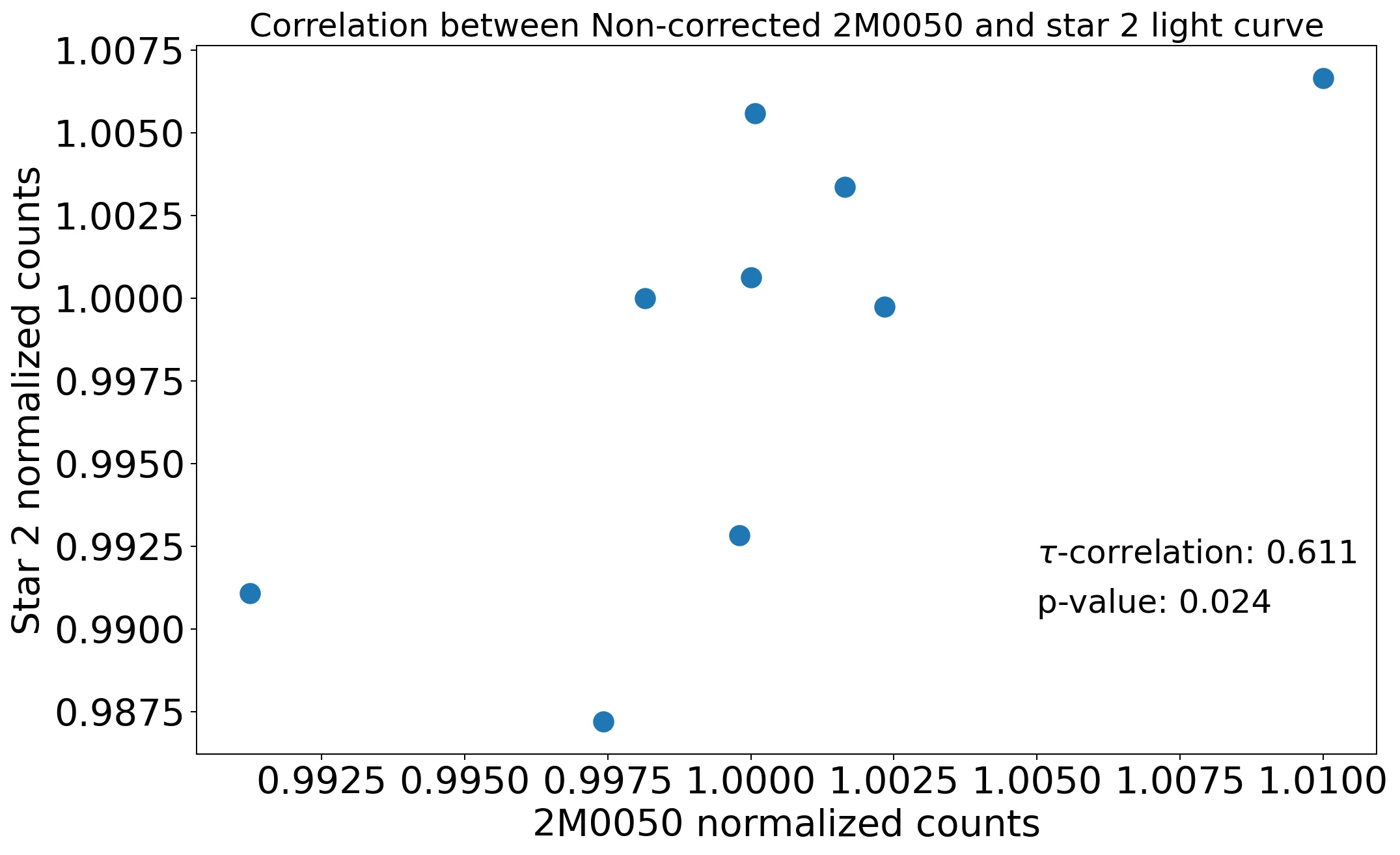
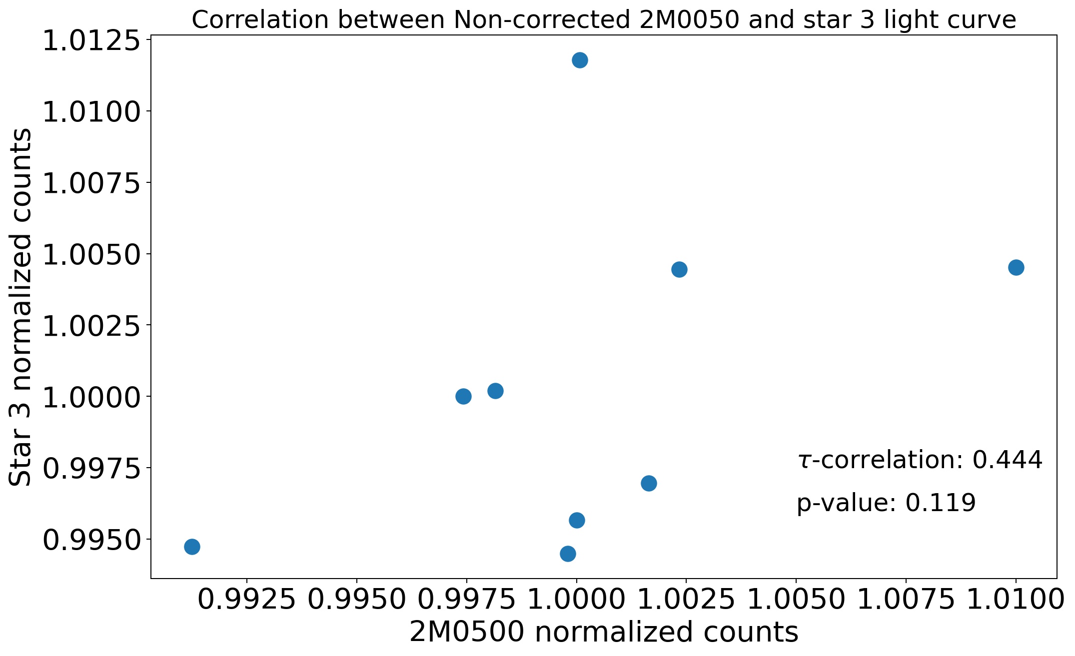
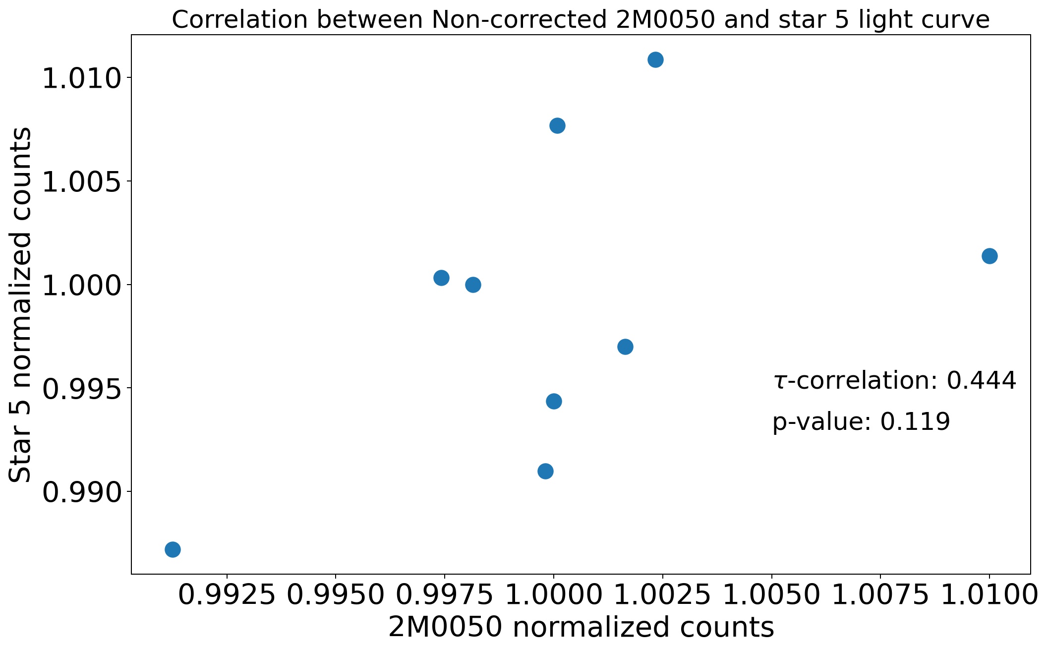
The Kendall’s $\tau$ coefficients suggests a weak to a moderate correlation between the $H$-band target’s and ”good” calibration stars light curves, depending on the star. The Kendall $\tau$ correlation coefficients vary between 0.44 (p-value = 0.12) for stars 1, 3 and 5, and 0.61 (p-value = 0.02) for the calibration star 2. In Fig. 18 in the Appendix, we show the correlation plots between the target and each of the stars that we use for calibration.

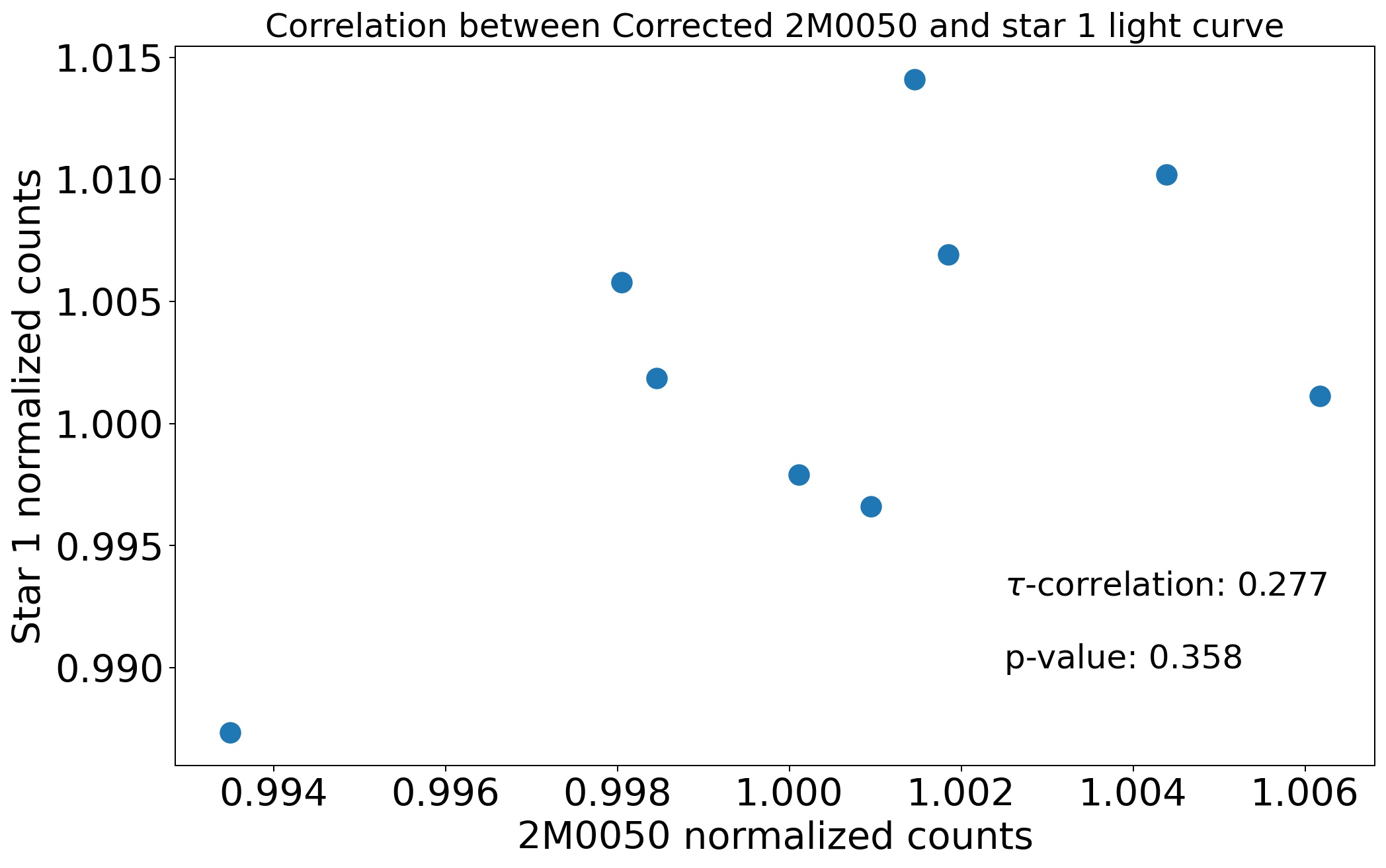
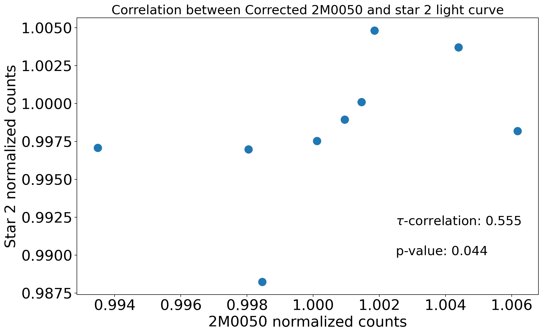
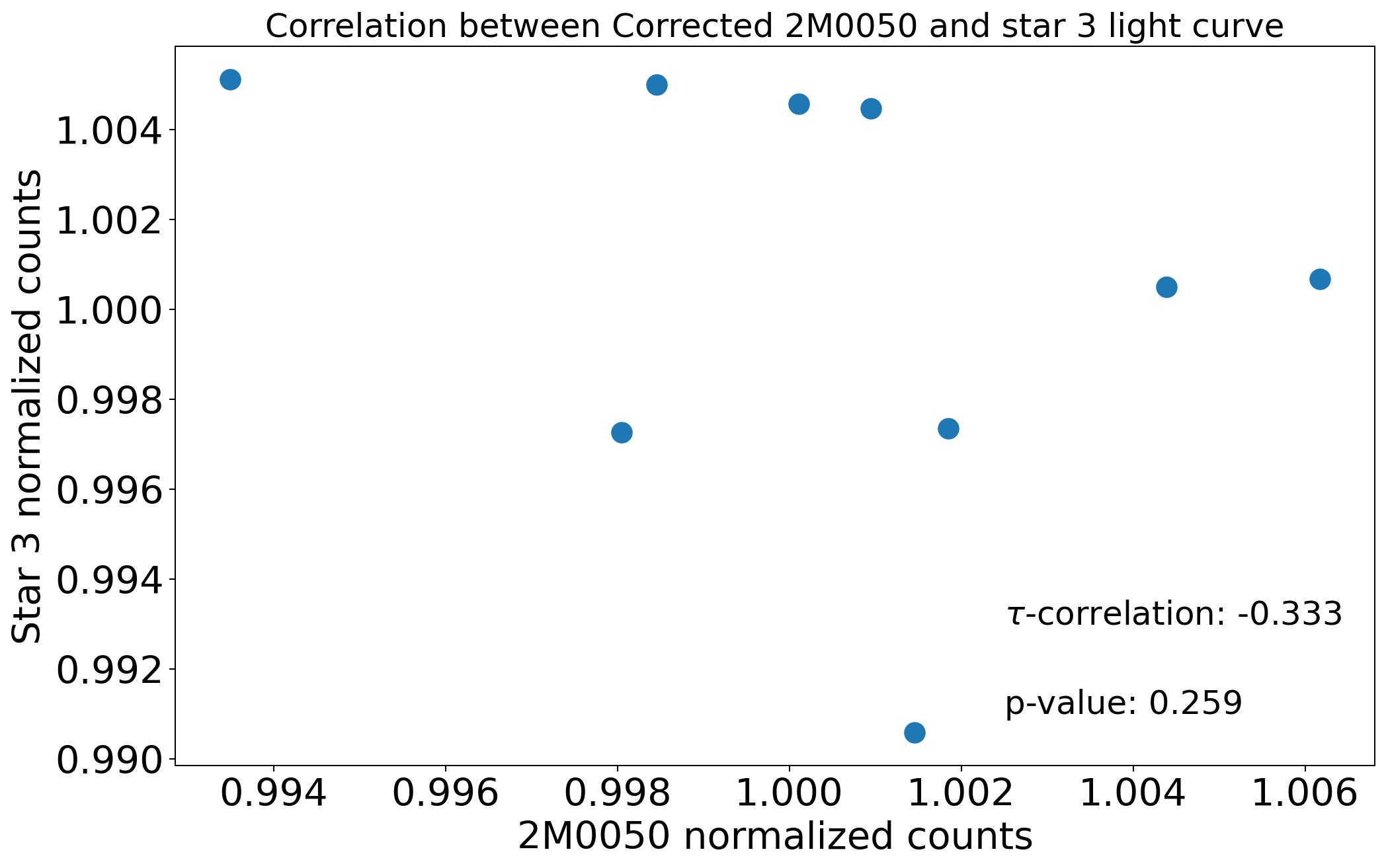
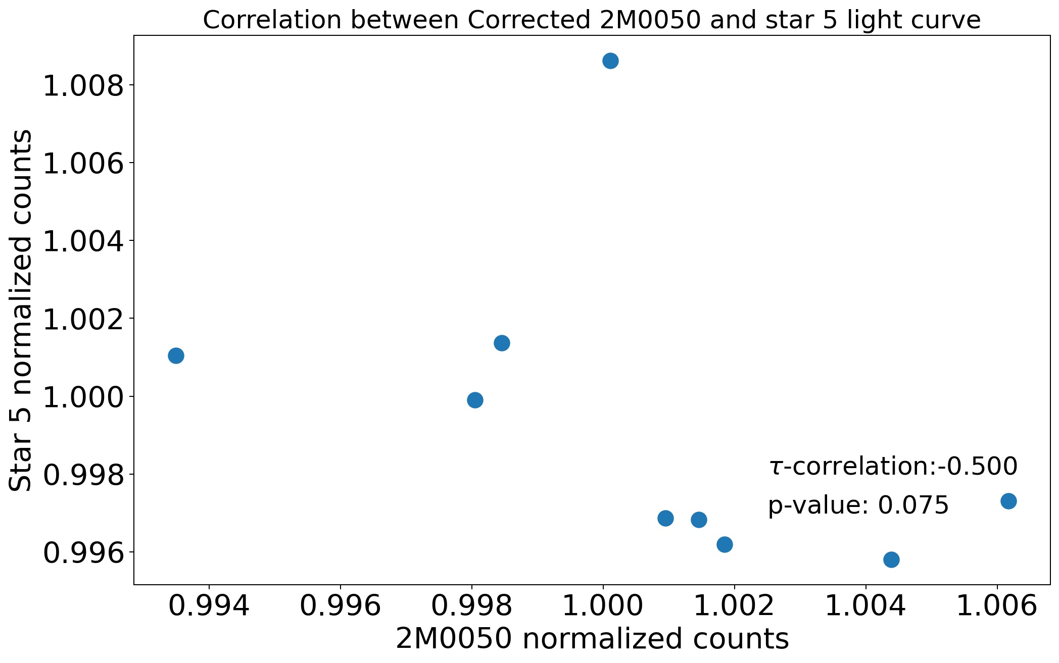
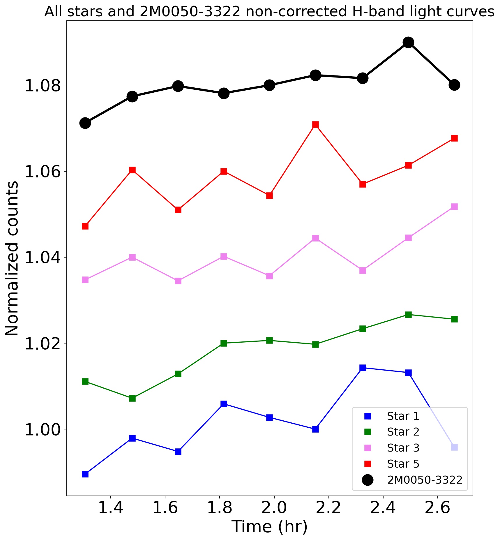
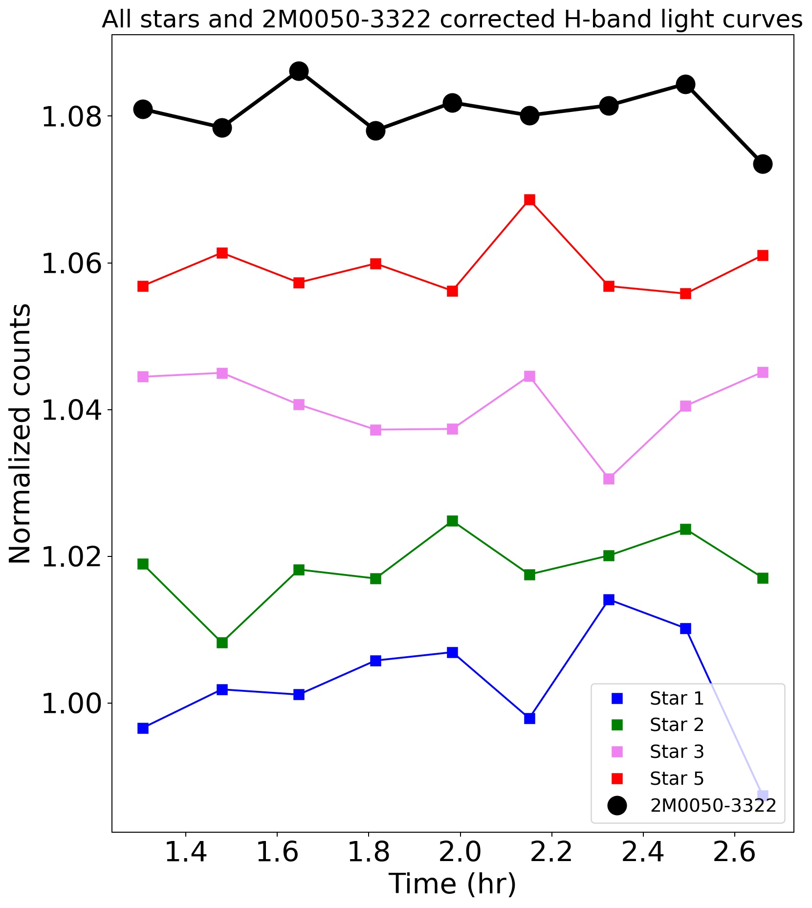
After correcting the light curves of 2M0050-3322 and the calibration stars using the method explained in Section 5, we run the Kendall $\tau$ non-parametric correlation test again, finding correlation coefficients that range between 0.28 (p-value = 0.37) for star 1, and 0.55 (p-value = 0.04) for the calibration star 2, suggesting non to a moderate correlation (see Fig. 19 in the Appendix). We show all stars and the target’s non-corrected and corrected light curves in Fig. 20 of the Appendix.

6.1.3 $\mathrm{CH_{4}-H_{2}O}$ region

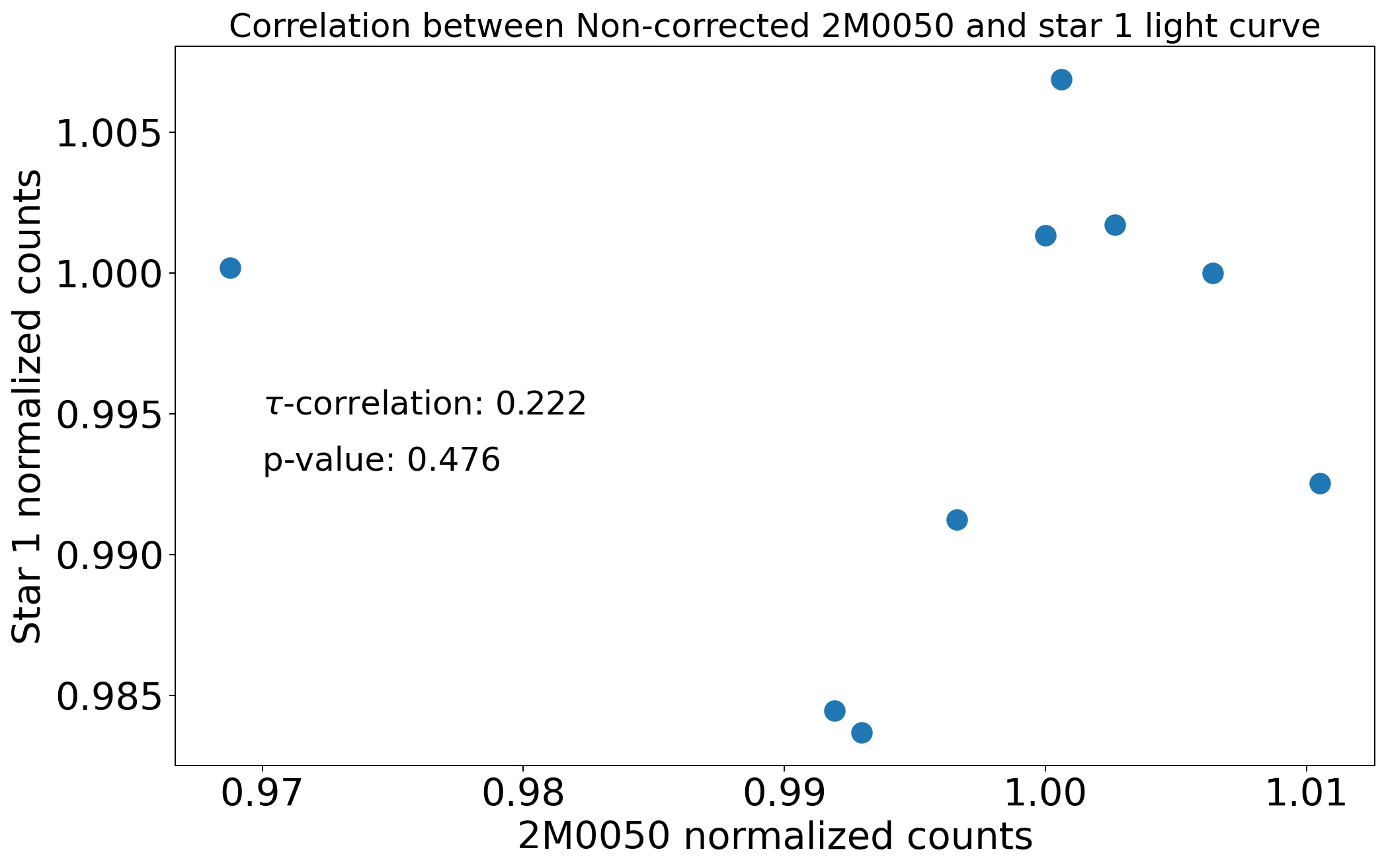
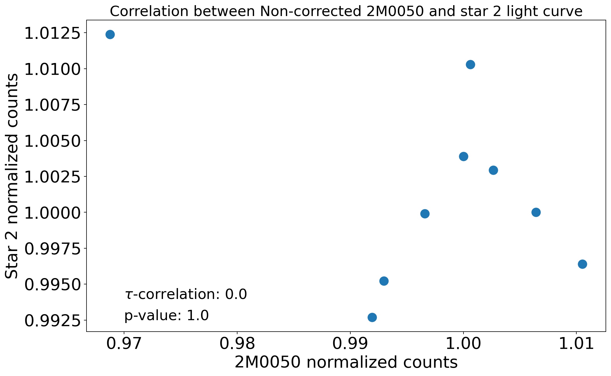
The Kendall’s $\tau$ coefficients suggests a weak correlation between the $\mathrm{CH_{4}-H_{2}O}$ target’s and ”good” calibration stars light curves, depending on the star. The Kendall $\tau$ correlation coefficients vary between 0.00 (p-value = 1.0) for star 2, and 0.22 (p-value = 0.47) for the calibration star 1. In Fig. 24 in the Appendix, we show the correlation plots between the target and the stars that we use for calibration.

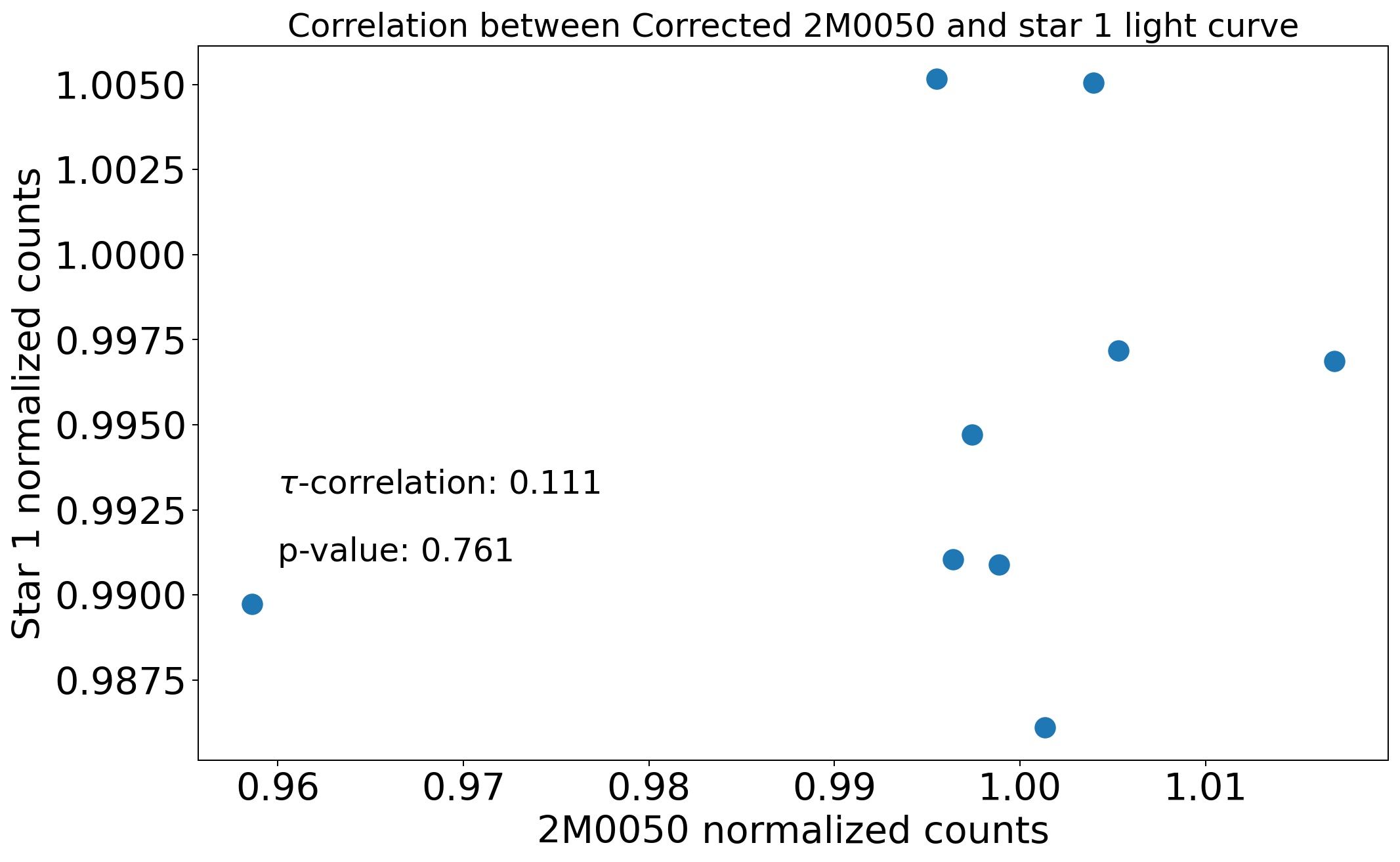
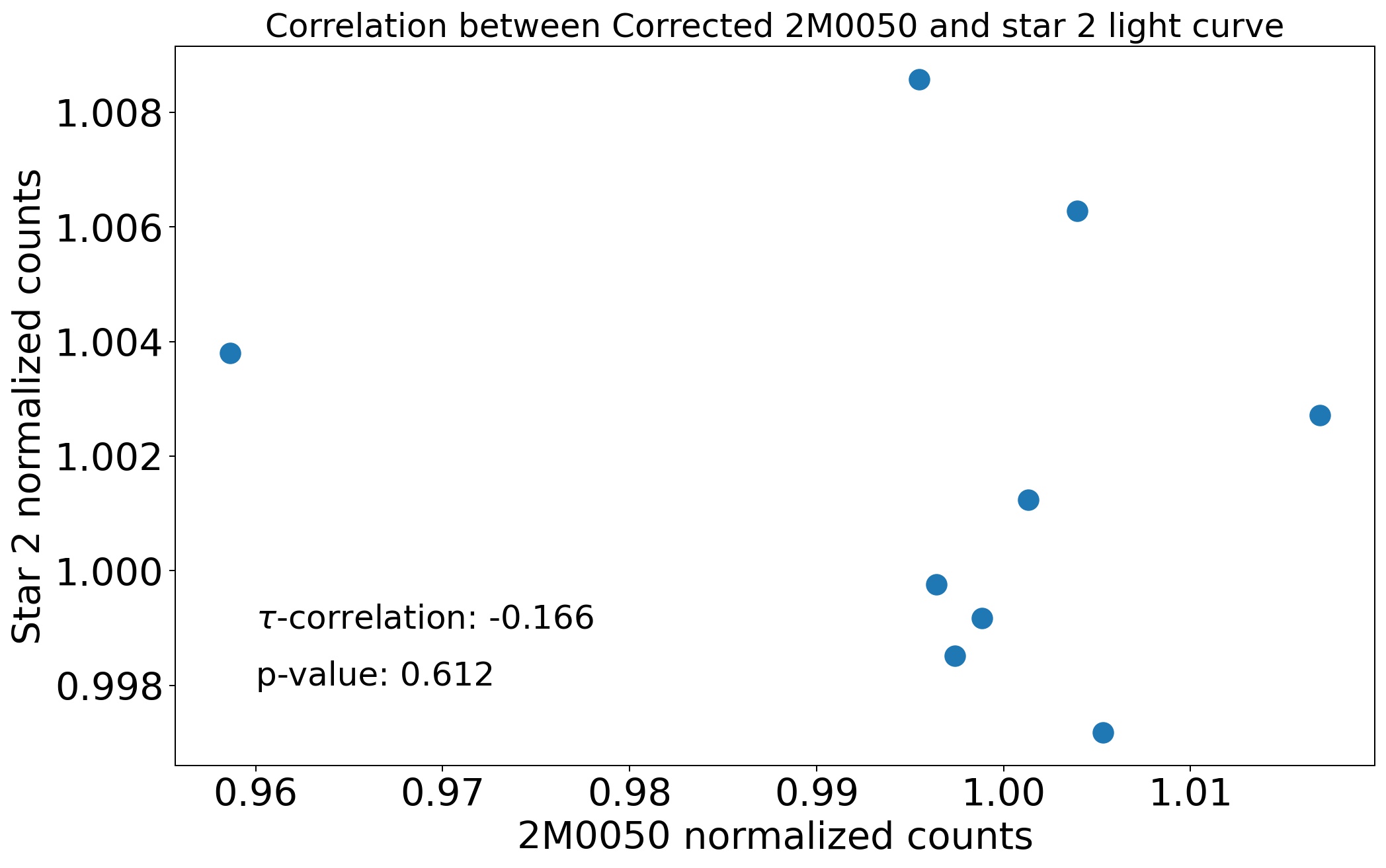
After correcting the light curves of 2M0050-3322 and the calibration stars using the method explained in Section 5, we run the Kendall $\tau$ non-parametric correlation test again, finding correlation coefficients of 0.11 (p-value = 0.76) for star 1, and -0.17 (p-value = 0.61) for star 2 (see Fig. 25 in the Appendix). We show the stars and the target’s non-corrected and corrected light curves in Fig. 25 of the Appendix.

6.2 Correlation with Full Width Half Maximum and centroids of the Spectra

For the $H$-band spectrophotometric data, we obtained spectra following an ABBA pattern. Thus, the slit losses might vary slightly at A and B positions, and also with the tracking of the telescope, and the flexure compensation of the instrument potentially influencing the measured variability of the target. These effects might be relevant since we observed at high airmasses (1.79–2.37). We investigated a potential relationship between the fluctuations found for 2M0050–3322, the Full Width Half Maximum (FWHM) of the 2D spectra, and centroids of those 2D spectra during the $\sim$1.4 hr of $H$-band monitoring with MOSFIRE. We do not perform this analysis for the $J$-band spectrophotometric data since we have only three data points. We do not perform this analysis at the $\mathrm{CH_{4}-H_{2}O}$ region, since the signal-to-noise is relatively low in this region.

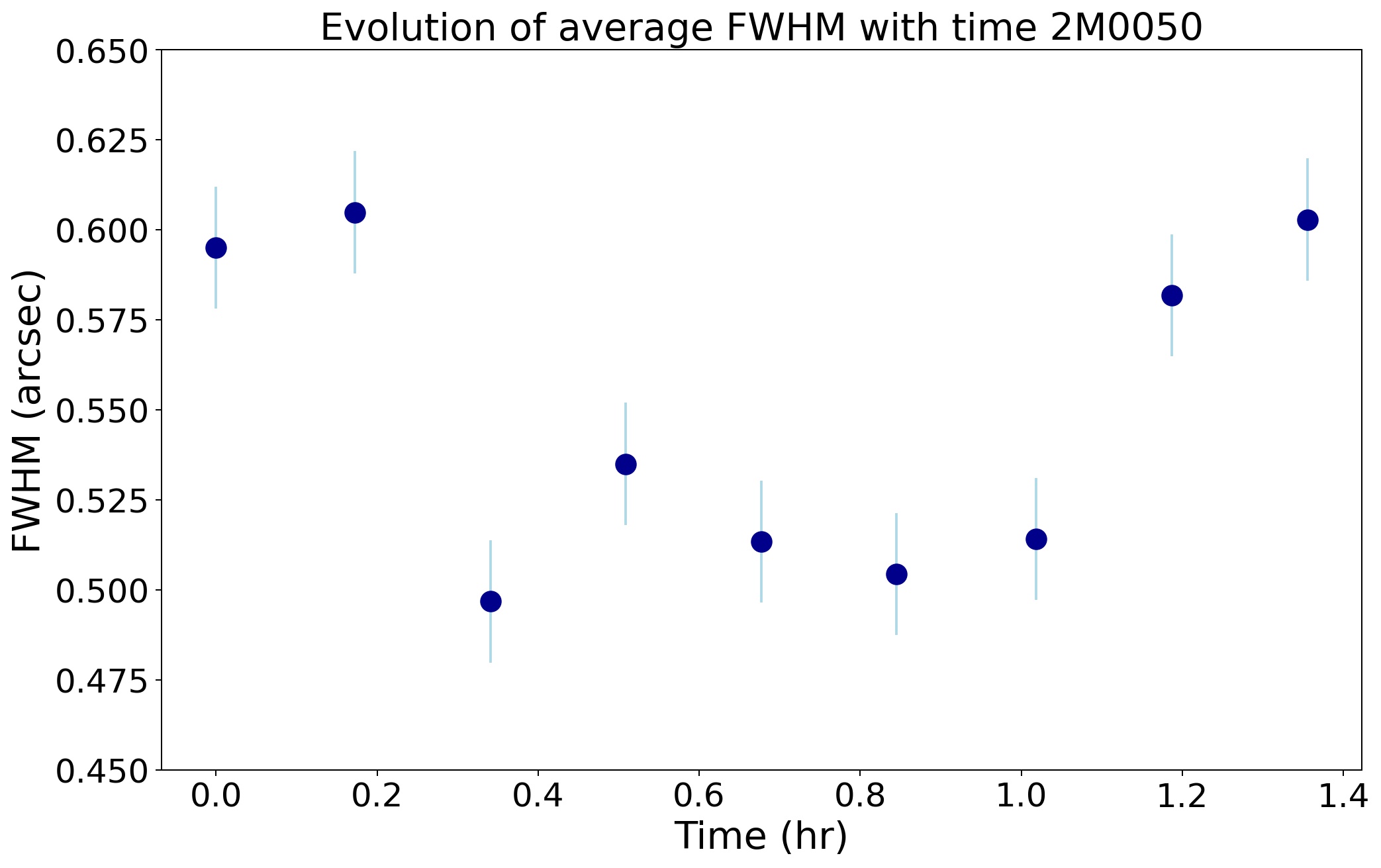
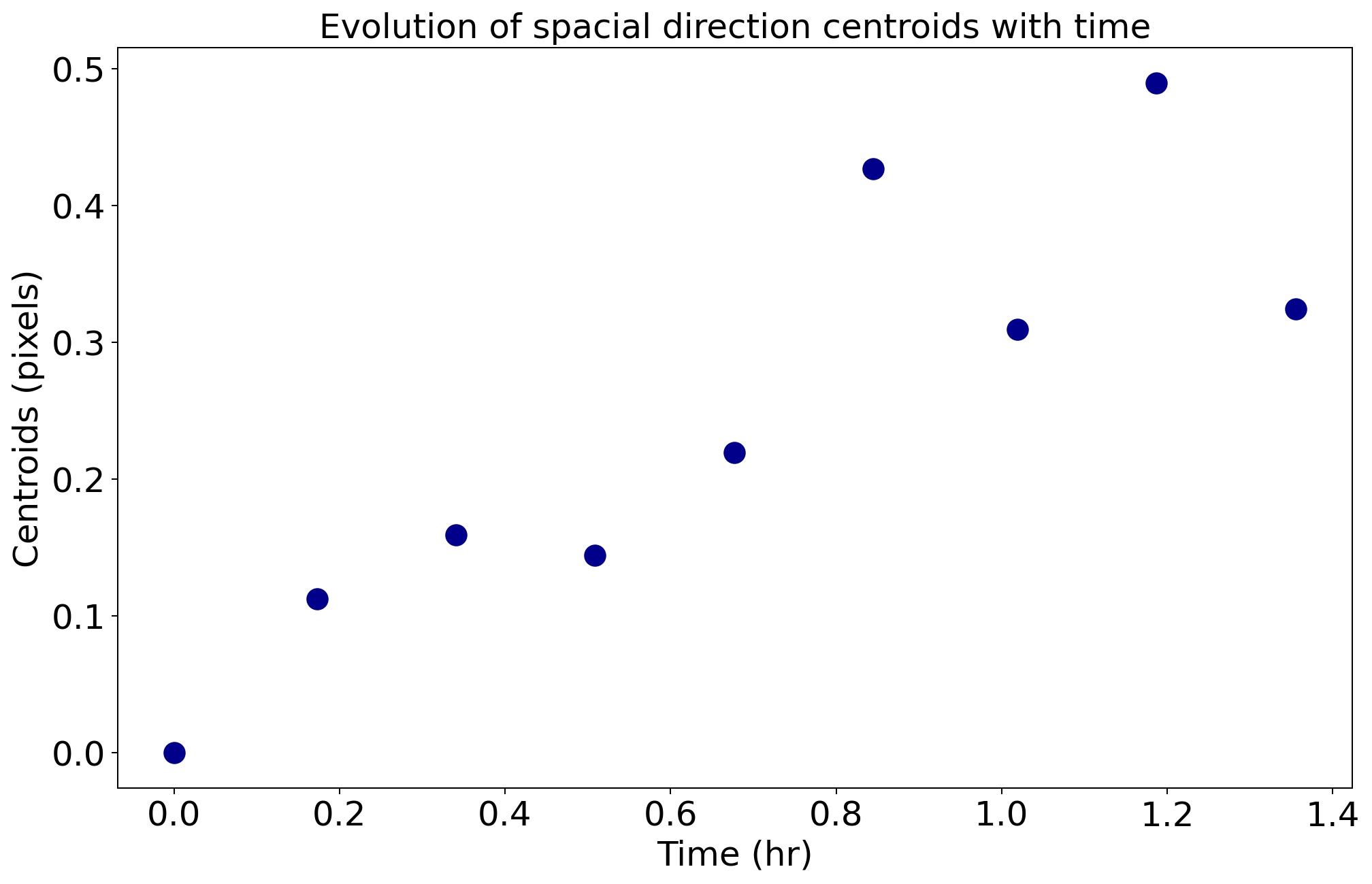
We measured the FWHM at approximately the maximum flux of coadded combined ABBA spectra between pixel x = 500, and pixel x = 550 (spatial direction), and then we calculated the FWHM at this position for each ABBA coadd using a 1D gaussian fit. We show the evolution of the FWHM in Fig. 21, left of the Appendix. Similarly, we calculated the centroids of the 2D spectra using the same gaussian fit (Fig. 21, right of the Appendix).

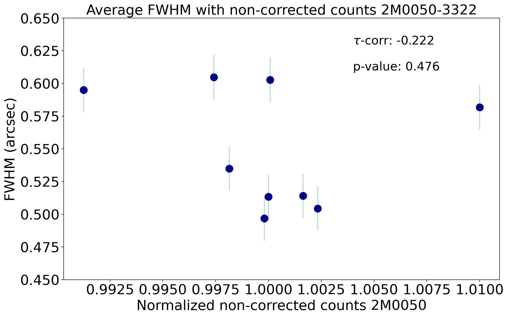
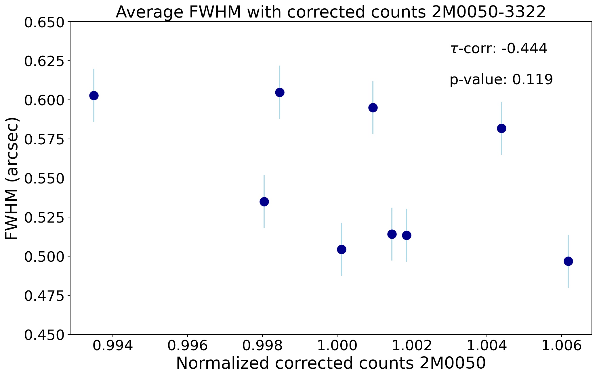
We calculated the Kendall $\tau$ correlation between the mean FWHM for each 2D spectrum and the non-corrected and corrected $H$-band light curve. We obtained a weak to moderate correlation between the FWHM and the non-corrected ($\tau$ = -0.22, p-value = 0.48) and corrected 2M0050–3322 light curves ($\tau$ = -0.44, p-value = 0.12). These correlations are shown in Fig. 22 of the Appendix.

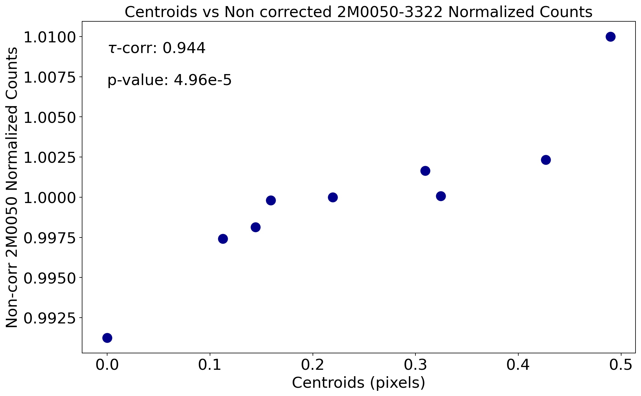
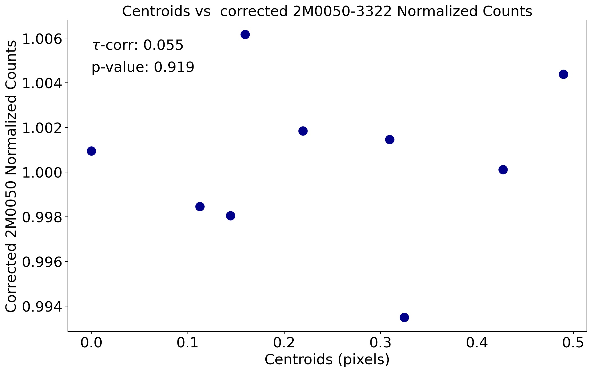
Finally, we obtained a strong correlation between the non-corrected 2M0050–3322 light curve and the measured centroids (centers as obtained from the 1D gaussian fit) of the 2D spectra ($\tau$ = 0.94, p-value = 4.9e-5). This correlation disappeared when we corrected the target’s light curve ($\tau$ = 0.06, p-value = 0.91), see Fig. 23 of the Appendix.

6.3 Correlation with Atmospherical Parameters

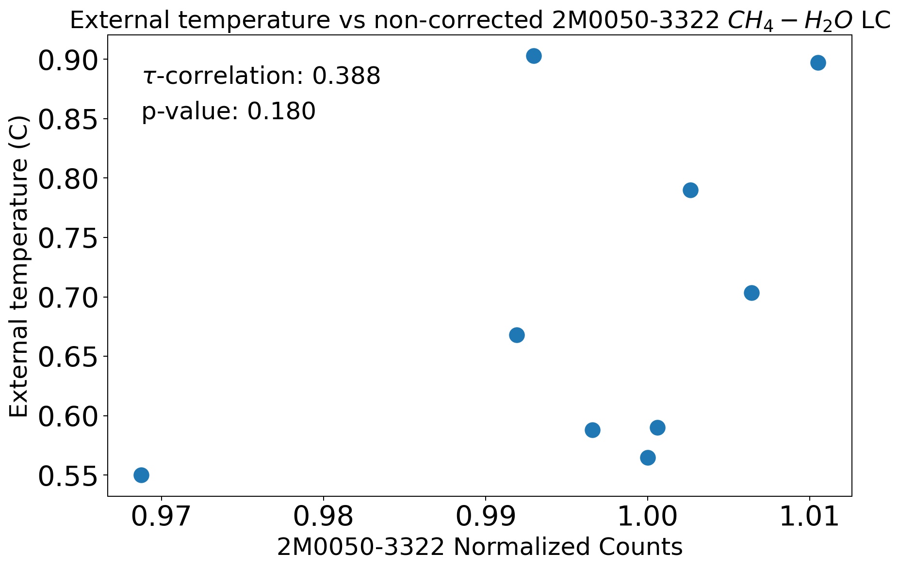
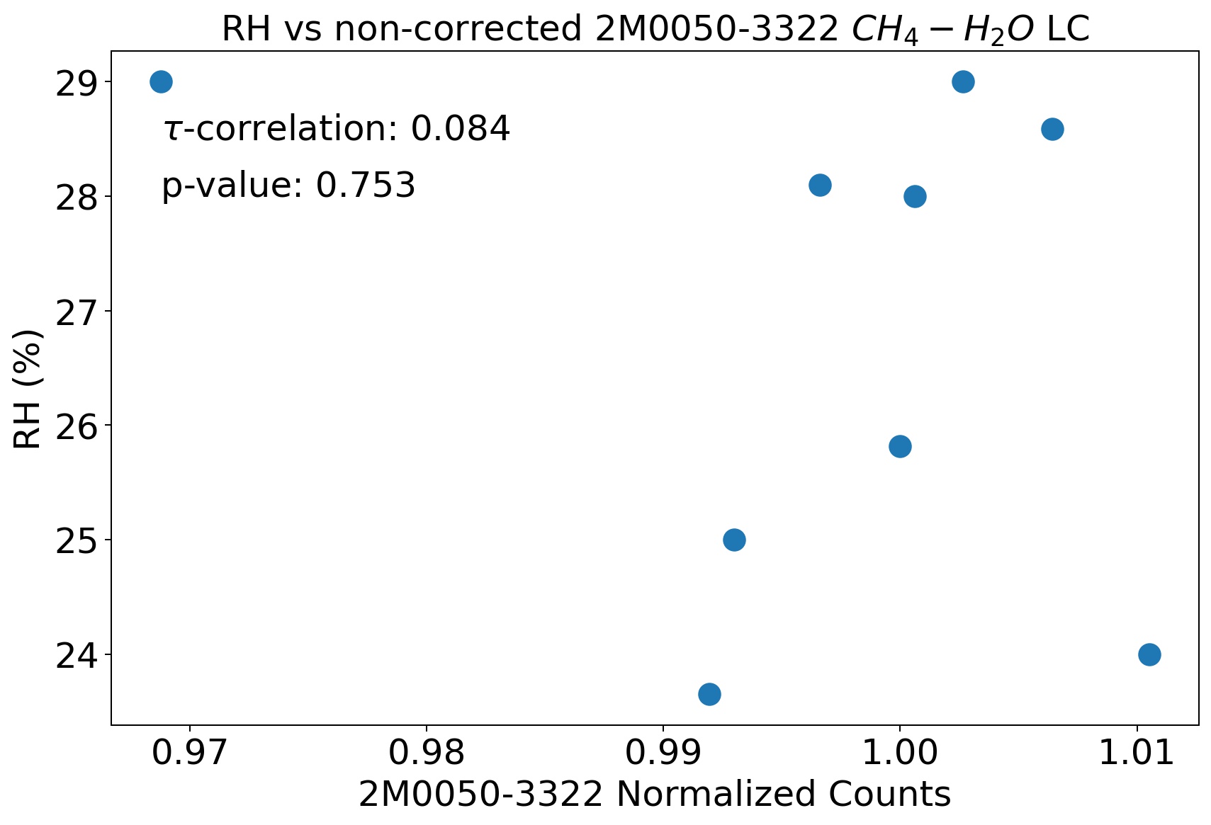
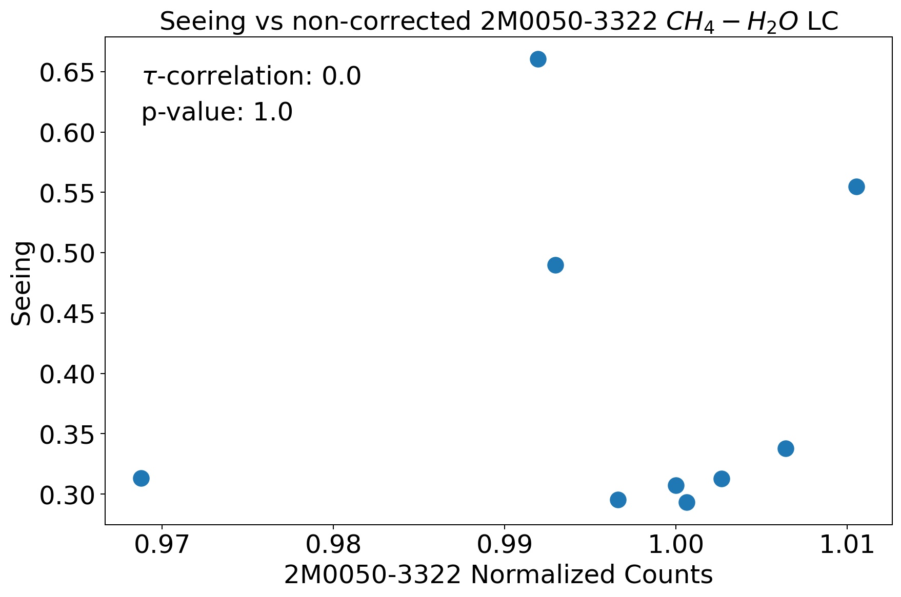
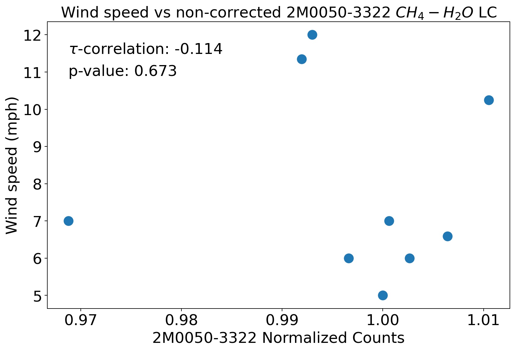
The evolution of atmospheric conditions during the observation might influence the amount of flux collected by MOSFIRE, affecting simultaneously the target and the calibration stars. Namely, the most relevant factors that might potentially affect our observations are: the humidity content, the external temperature, wind speed, seeing and the airmass. The evolution of these parameters are registered in the header, and/or in the Mauna Kea Weather Center webpage (http://mkwc.ifa.hawaii.edu).

6.3.1 $J$-band light curves

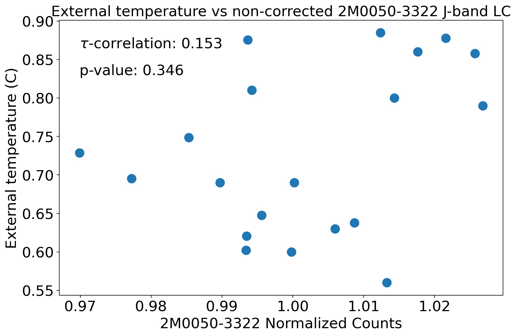
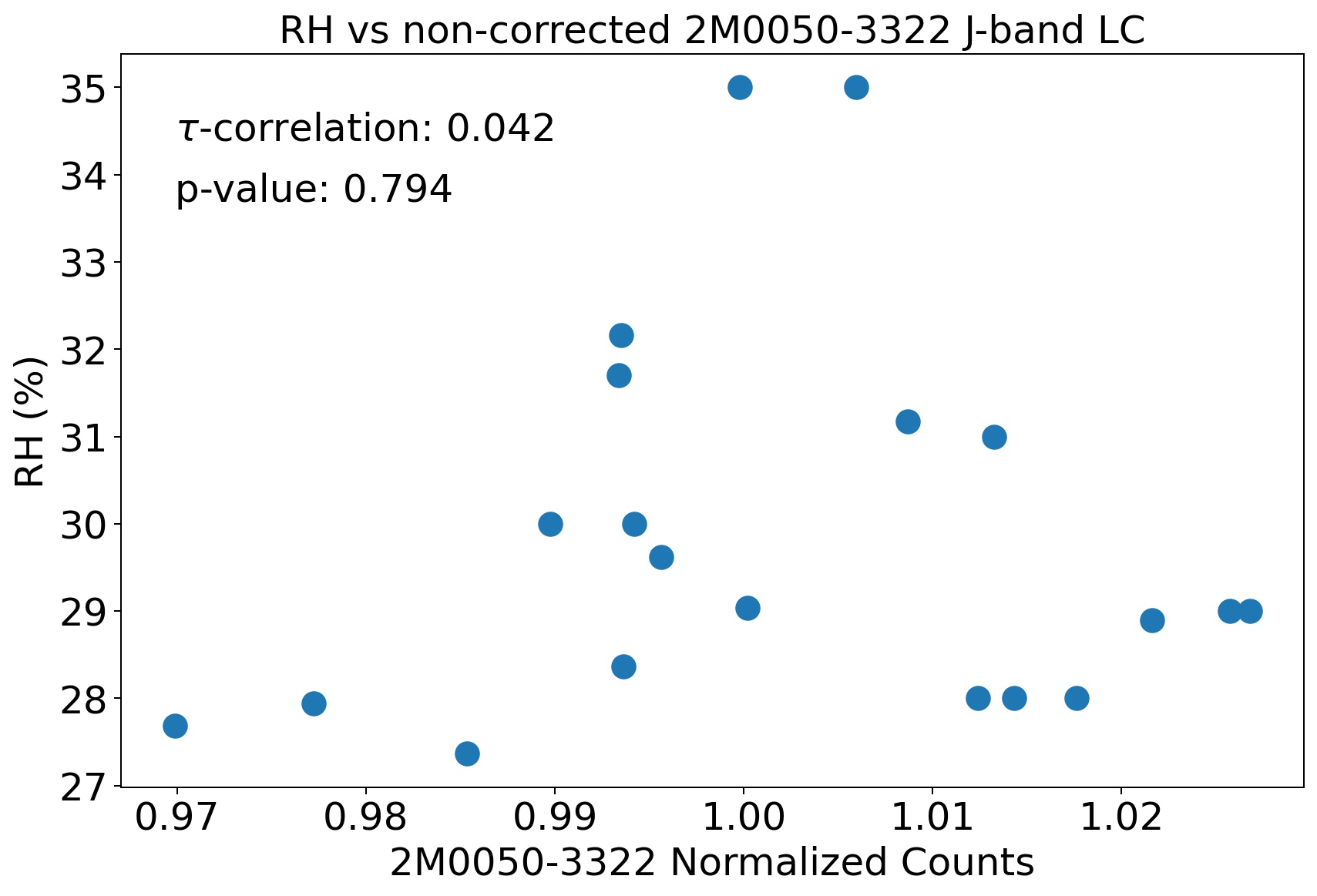
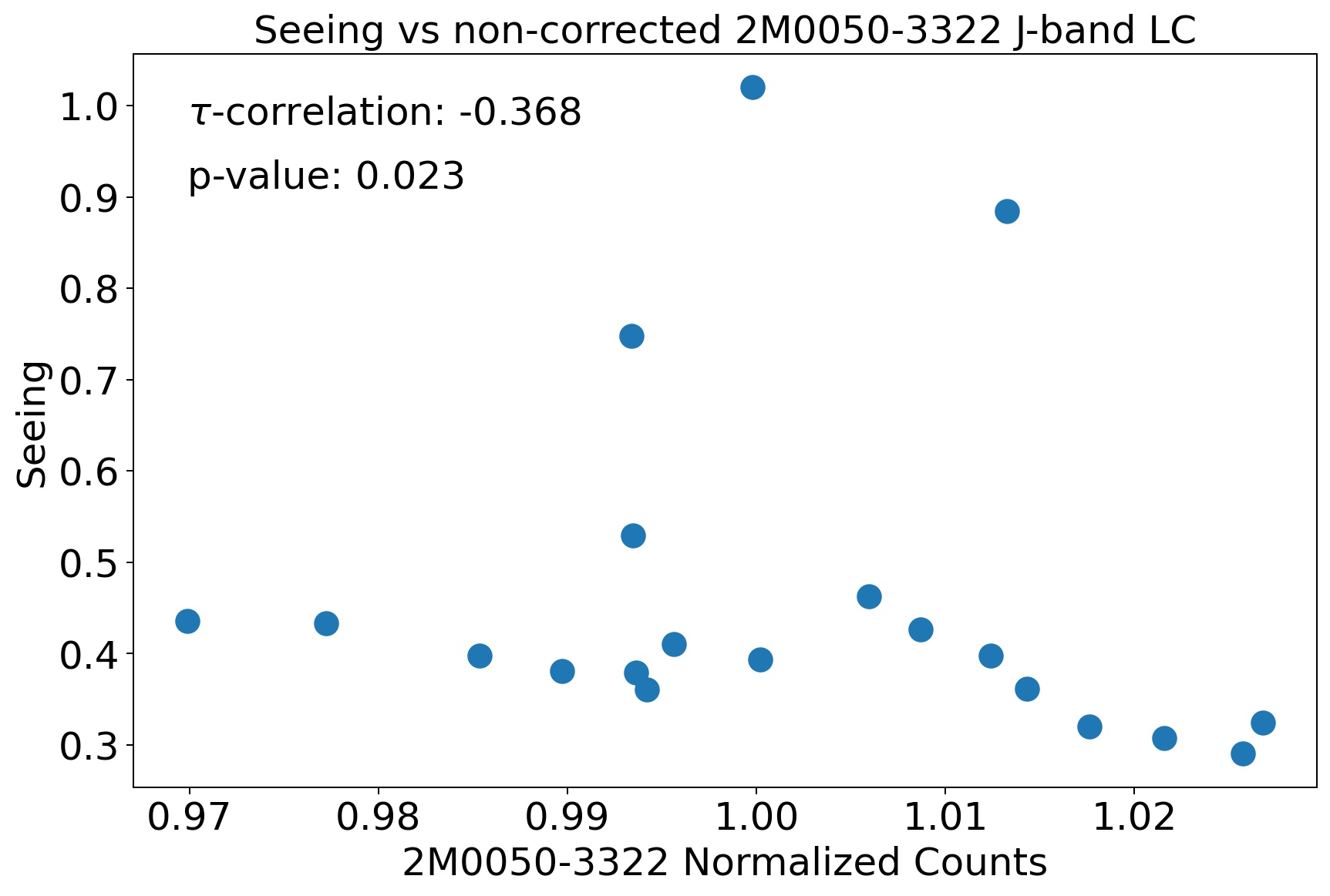
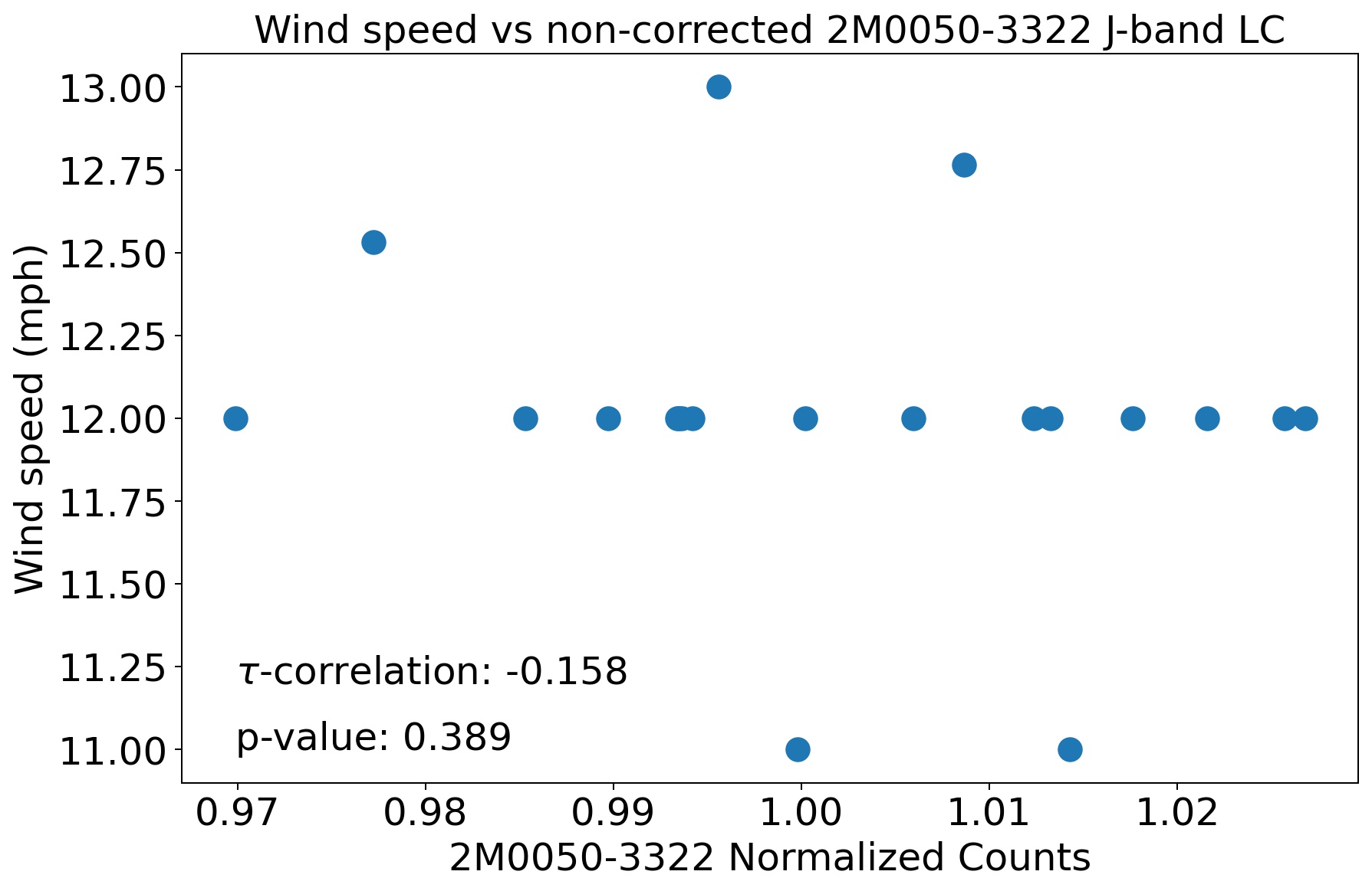
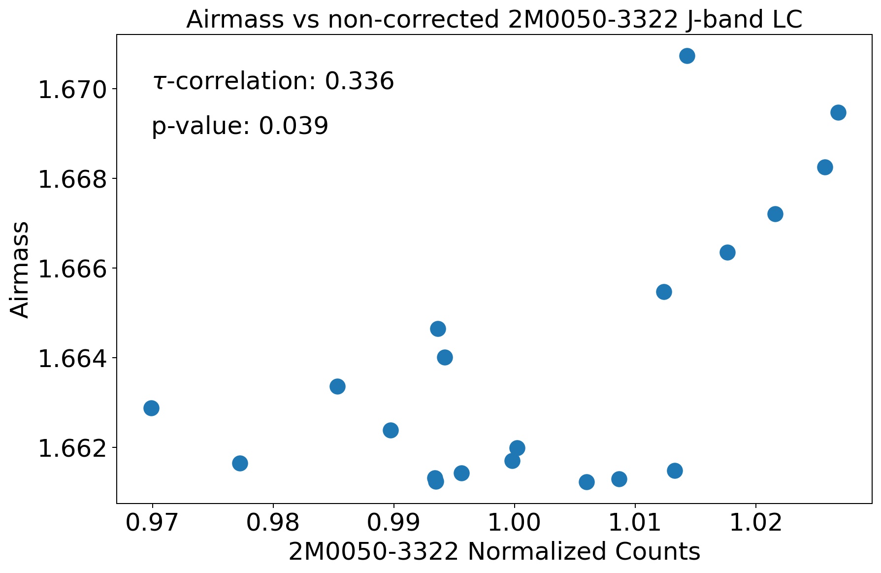
We calculated the $\tau$ Kendall correlation coefficient between the non-corrected and the corrected $J$-band imaging light curve for 2M0050–3322, and each of the atmospheric parameters mentioned above. We found no to weak correlation between the non-corrected $J$-band target’s light curve and the humidity content ($\tau$ = 0.04, p-value = 0.79), the external temperature ($\tau$ = 0.15, p-value = 0.35), and wind speed ($\tau$ = -0.16, p-value = 0.39). We found a weak correlation with the seeing ($\tau$ = -0.37, p-value = 0.023), and with the airmass ($\tau$ = 0.34, p-value = 0.04). The plot showing all correlations can be found in Fig. 26 in the Appendix. We did not find any correlation between the corrected $J$-band imaging light curve and the atmospheric parameters, as can be seen in Fig. 27 in the Appendix.

6.3.2 $H$-band light curves

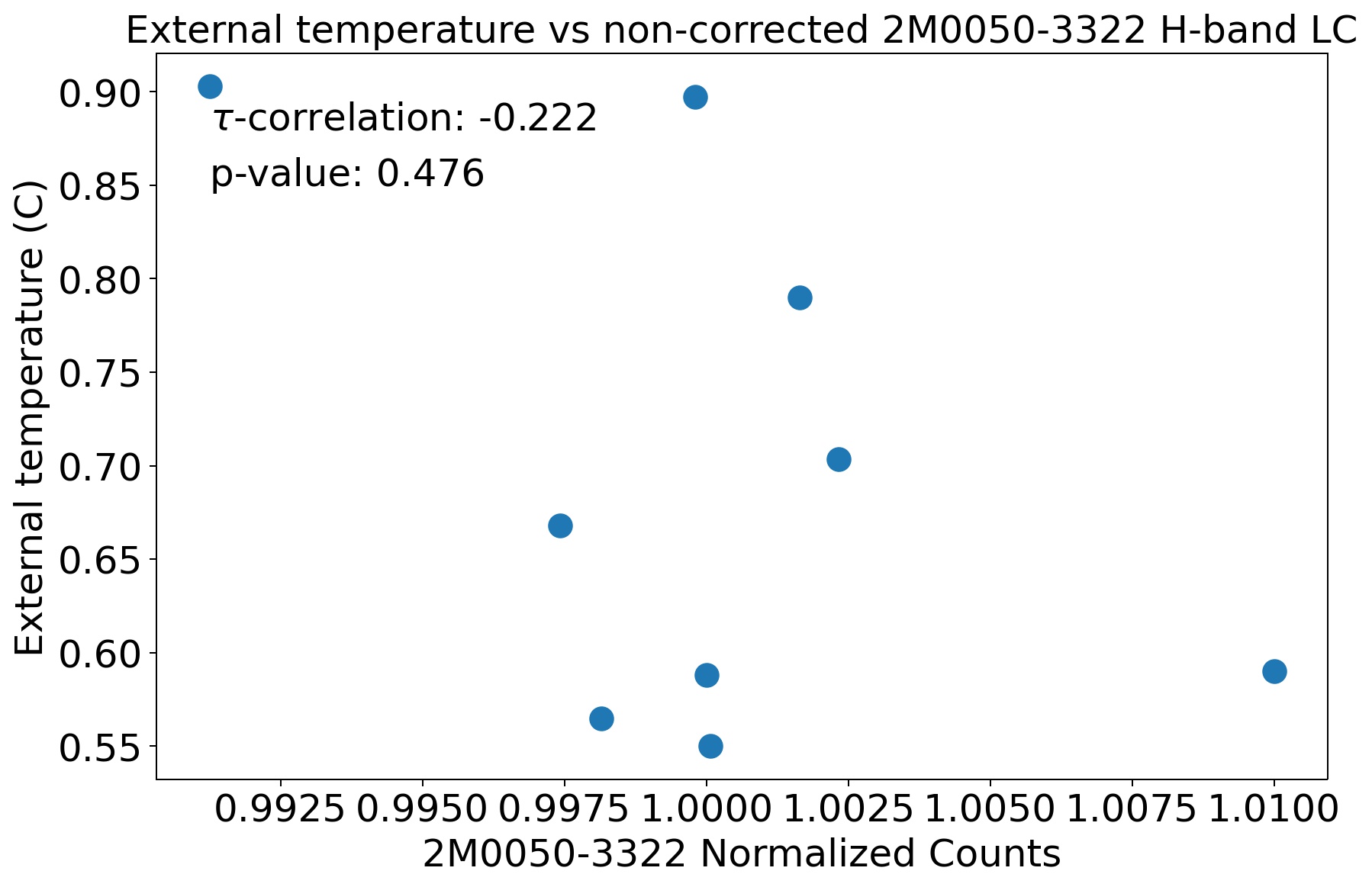
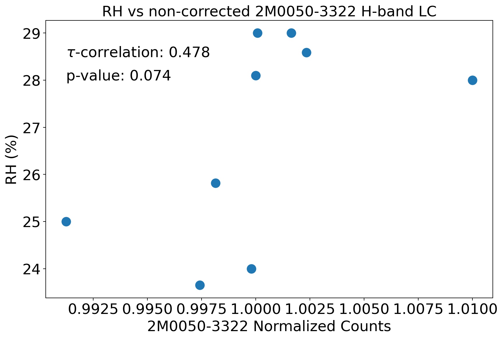
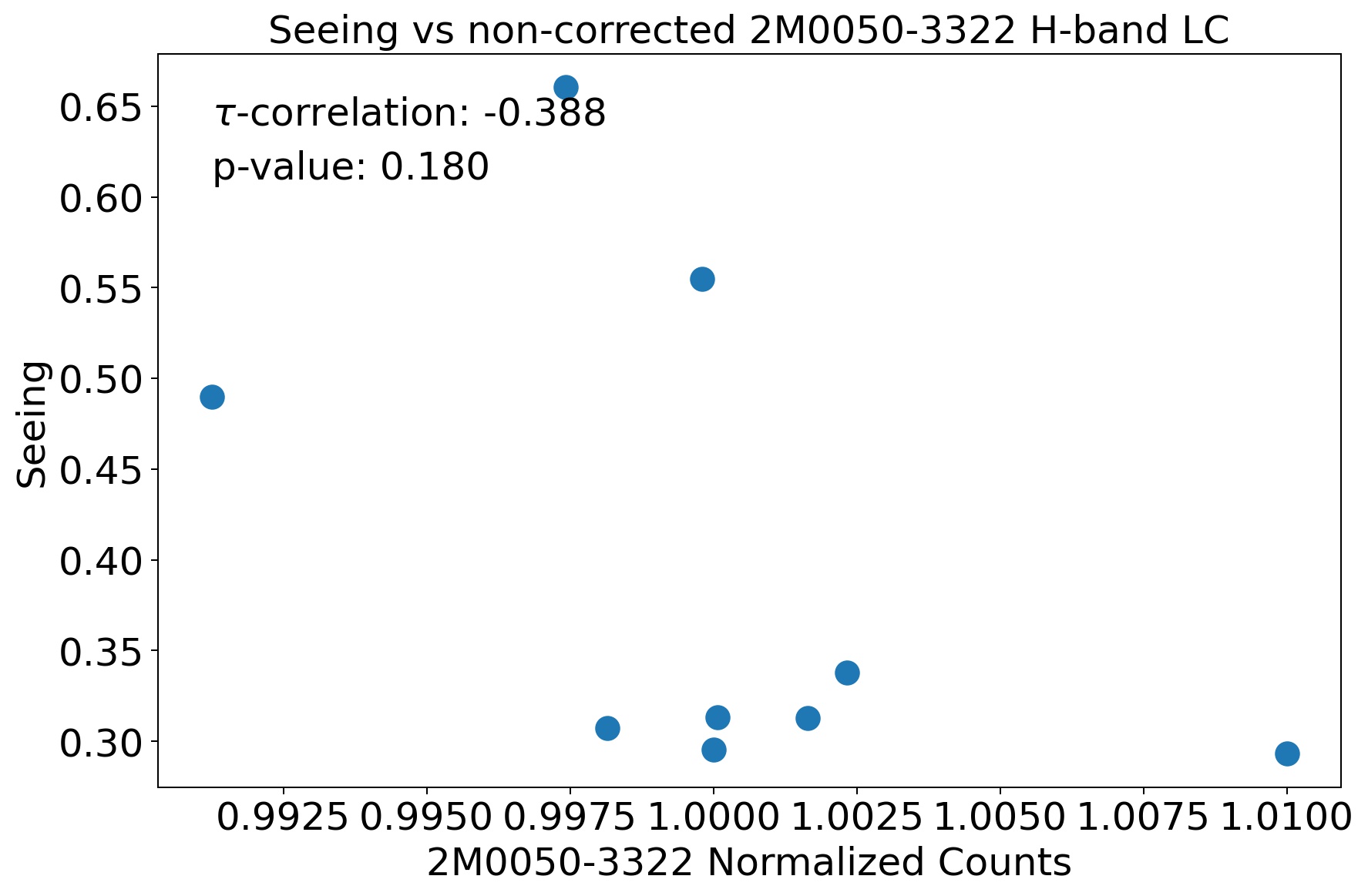
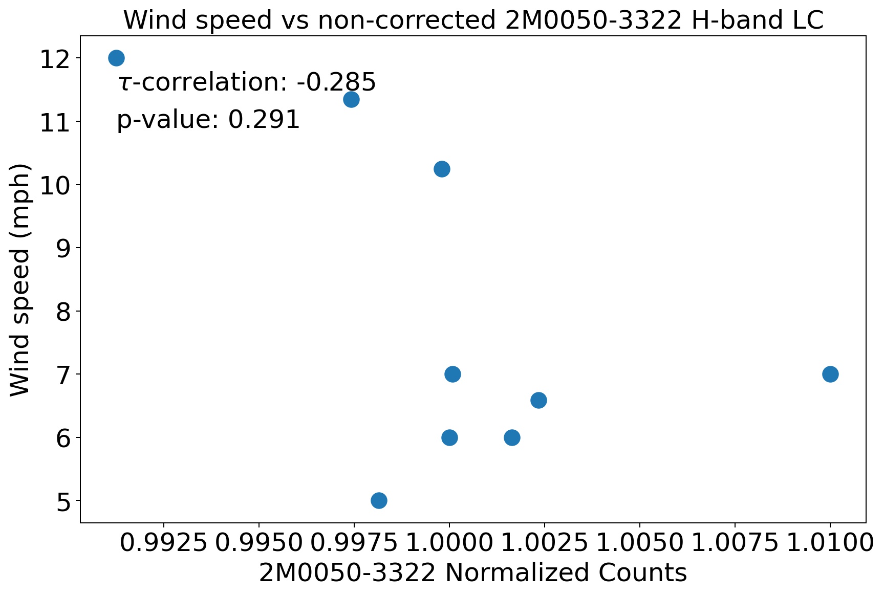
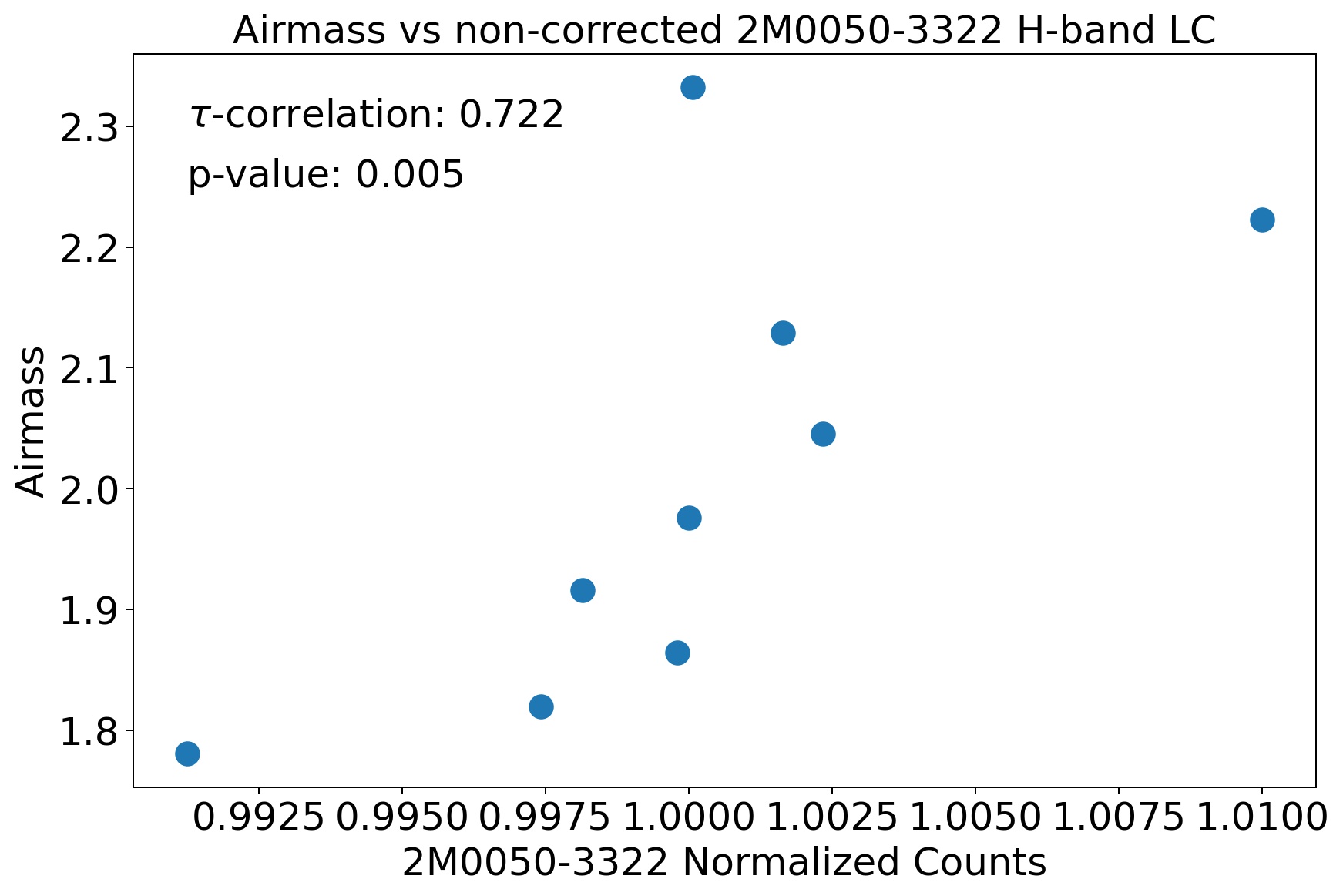
We calculated the $\tau$ Kendall correlation coefficient between the non-corrected, and corrected $H$-band spectrophotometric light curves for 2M0050–3322, and each of the atmospheric parameters mentioned above. We found a strong correlation between the airmass and the non-corrected $H$-band light curve of 2M0050–3322 ($\tau$ = 0.72, p-value = 0.005), a moderate correlation with the humidity content ($\tau$ = 0.48, p-value = 0.07), and a weak anticorrelation with the seeing ($\tau$ = -0.39, p-value = 0.18), the wind speed ($\tau$ = -0.29, p-value = 0.29), and the external temperature ($\tau$ = -0.22, p-value = 0.48). The correlation plots can be found in Fig. 28 of the Appendix.

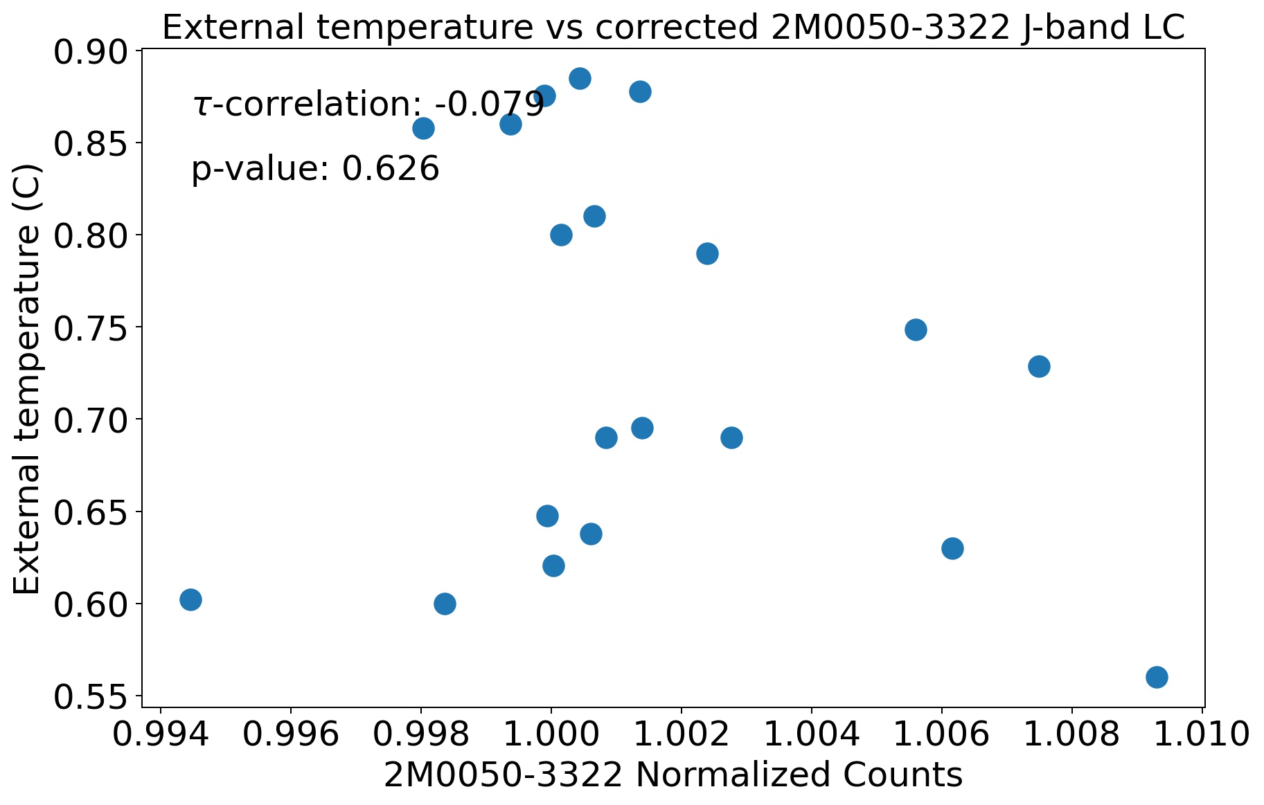
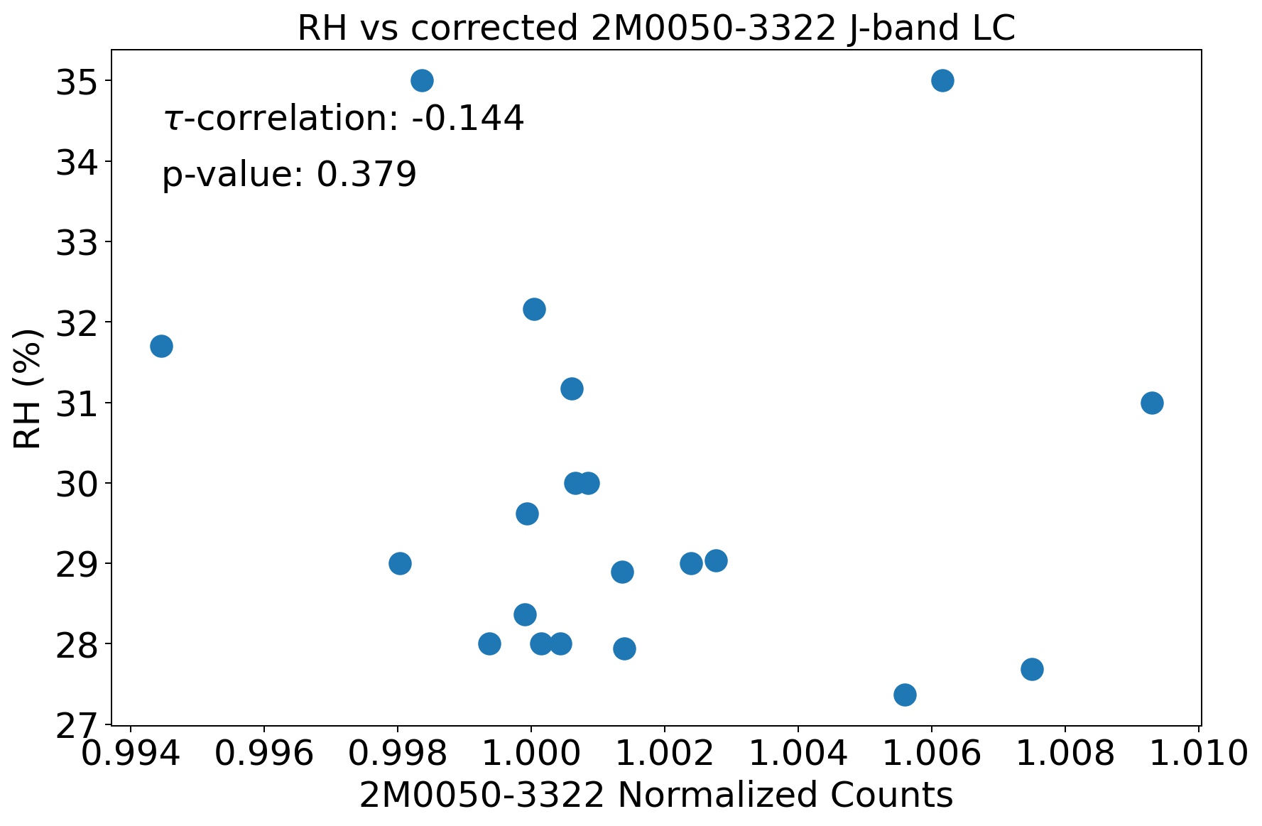
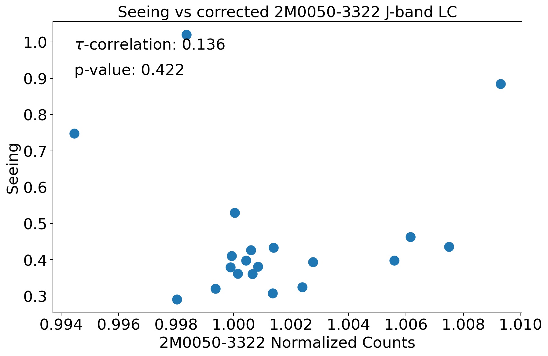
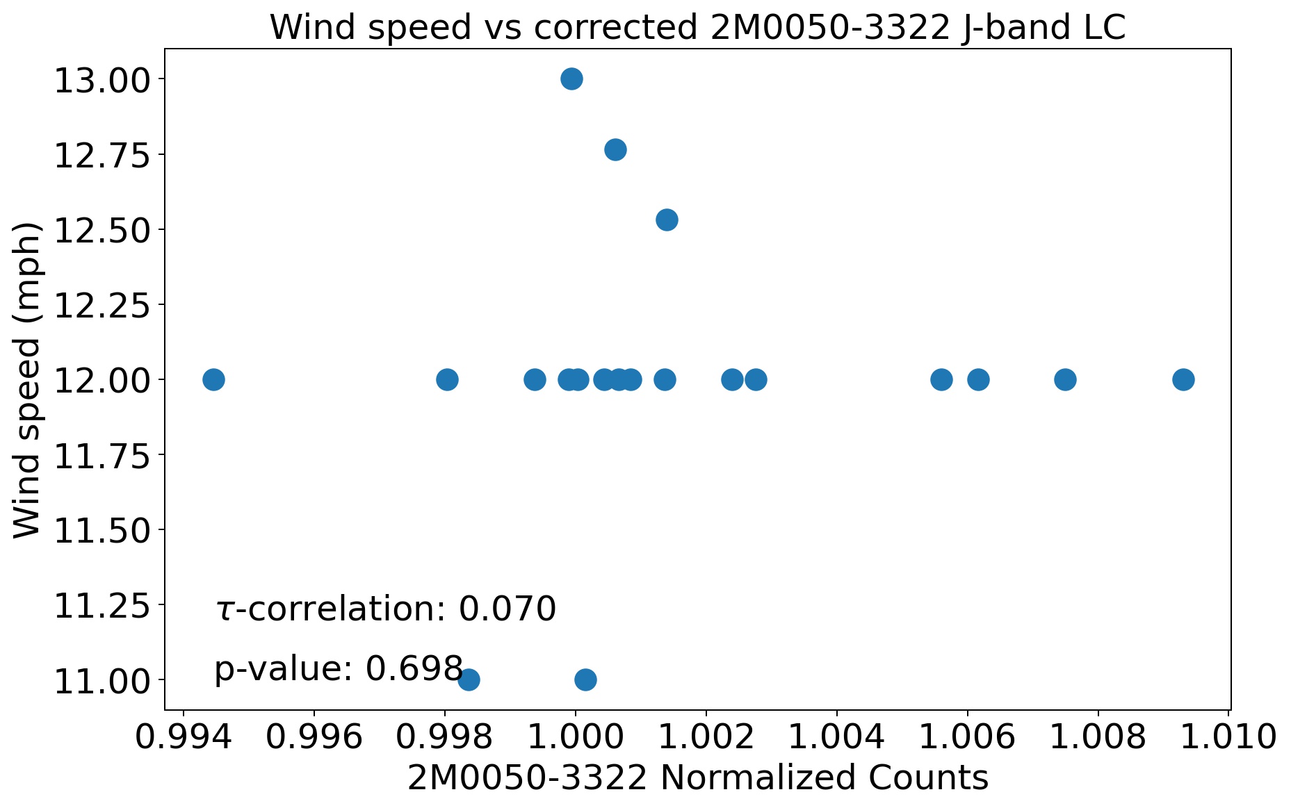
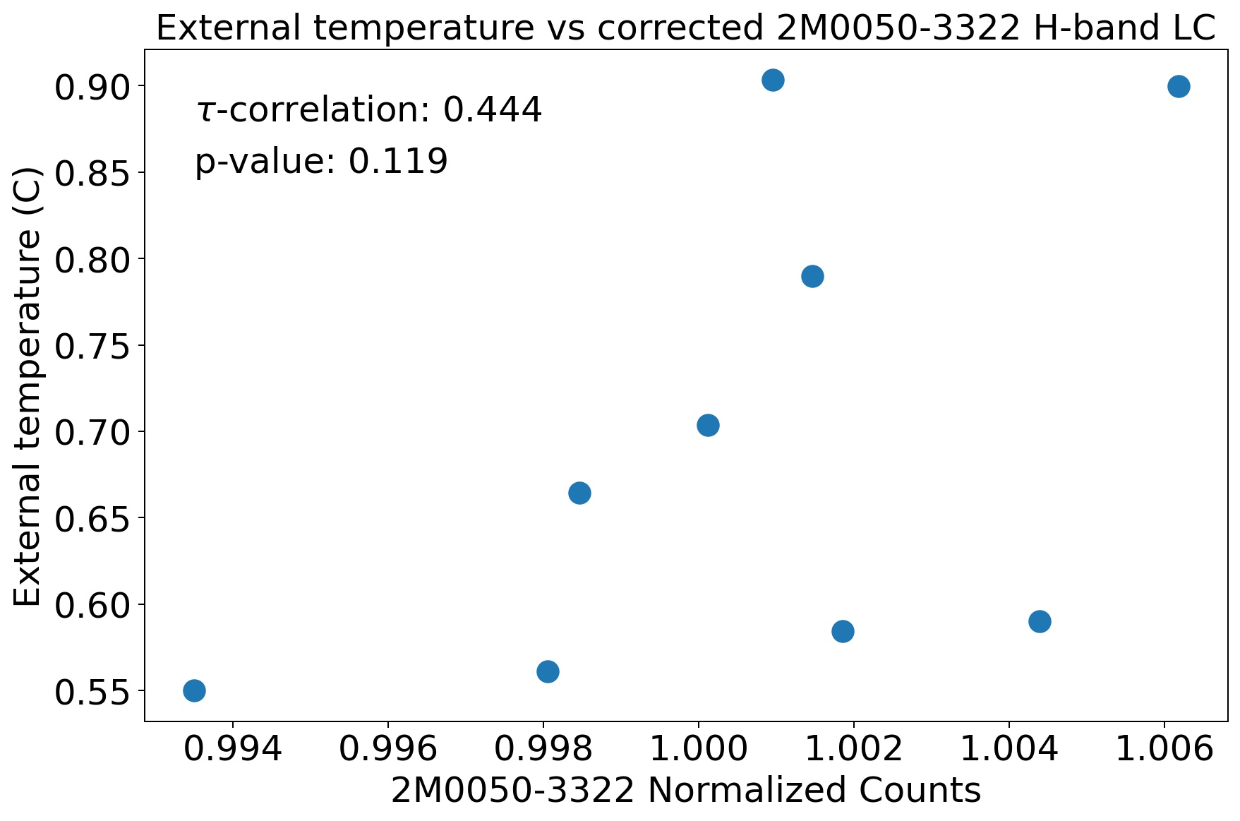
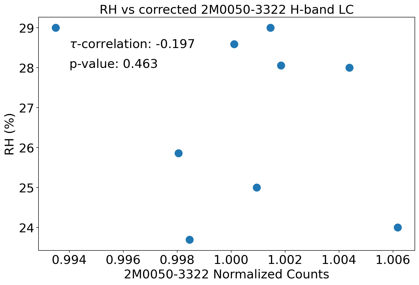
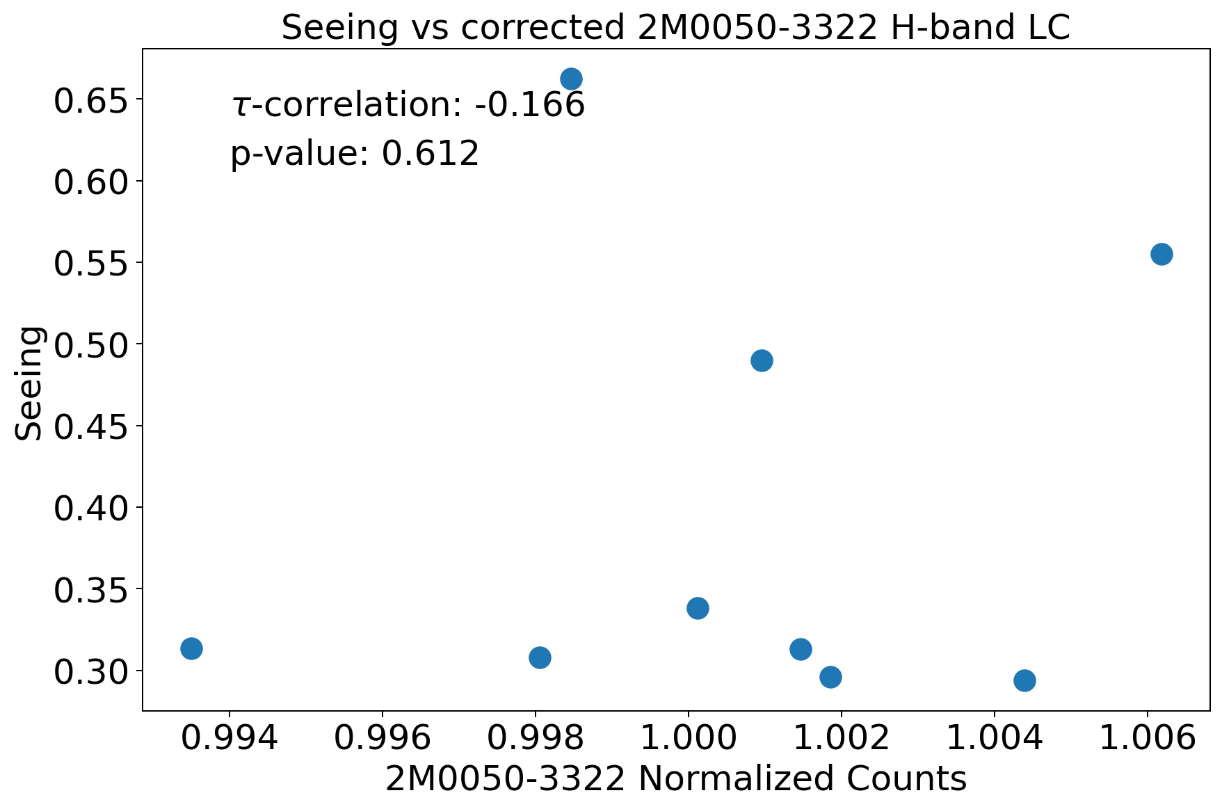
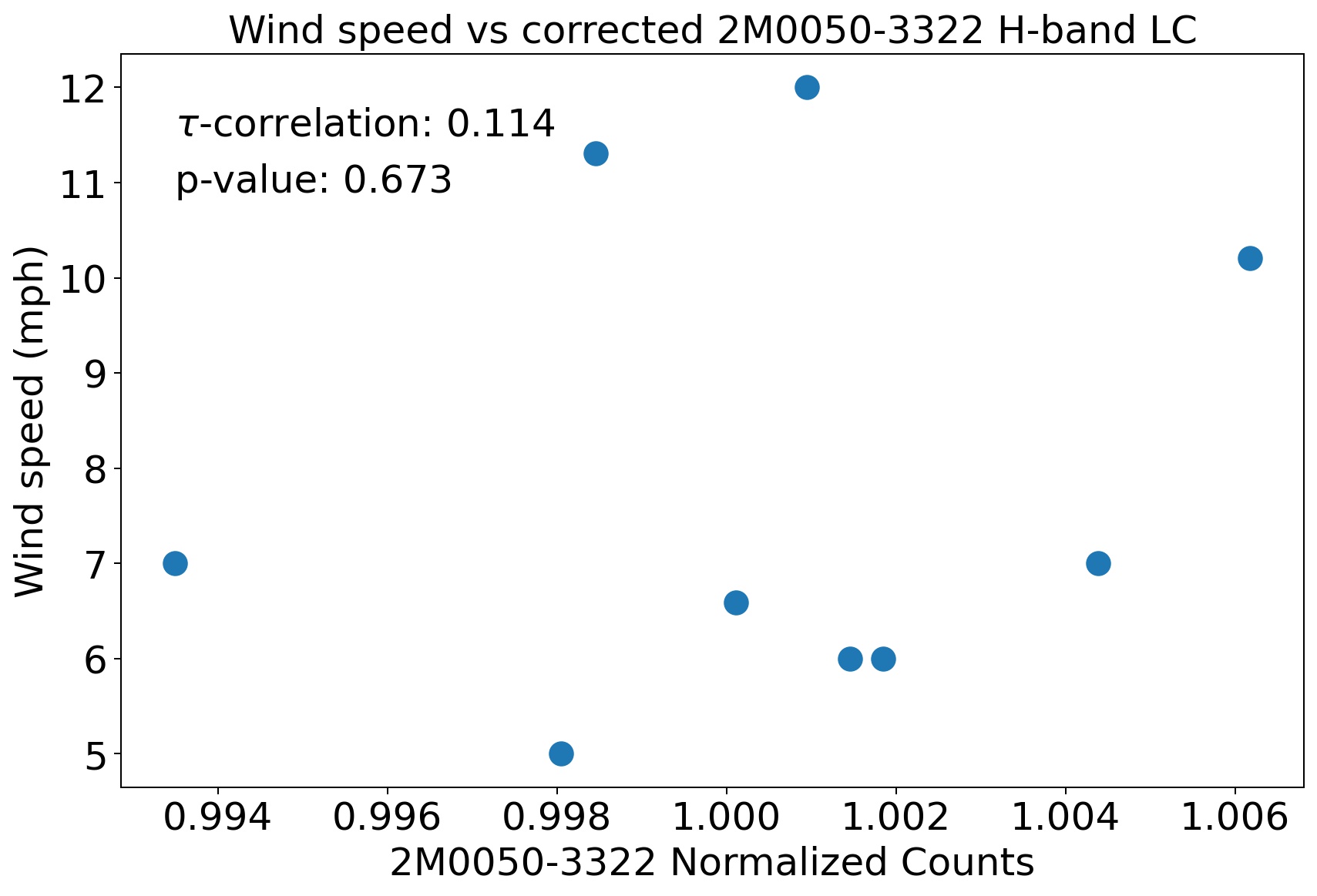
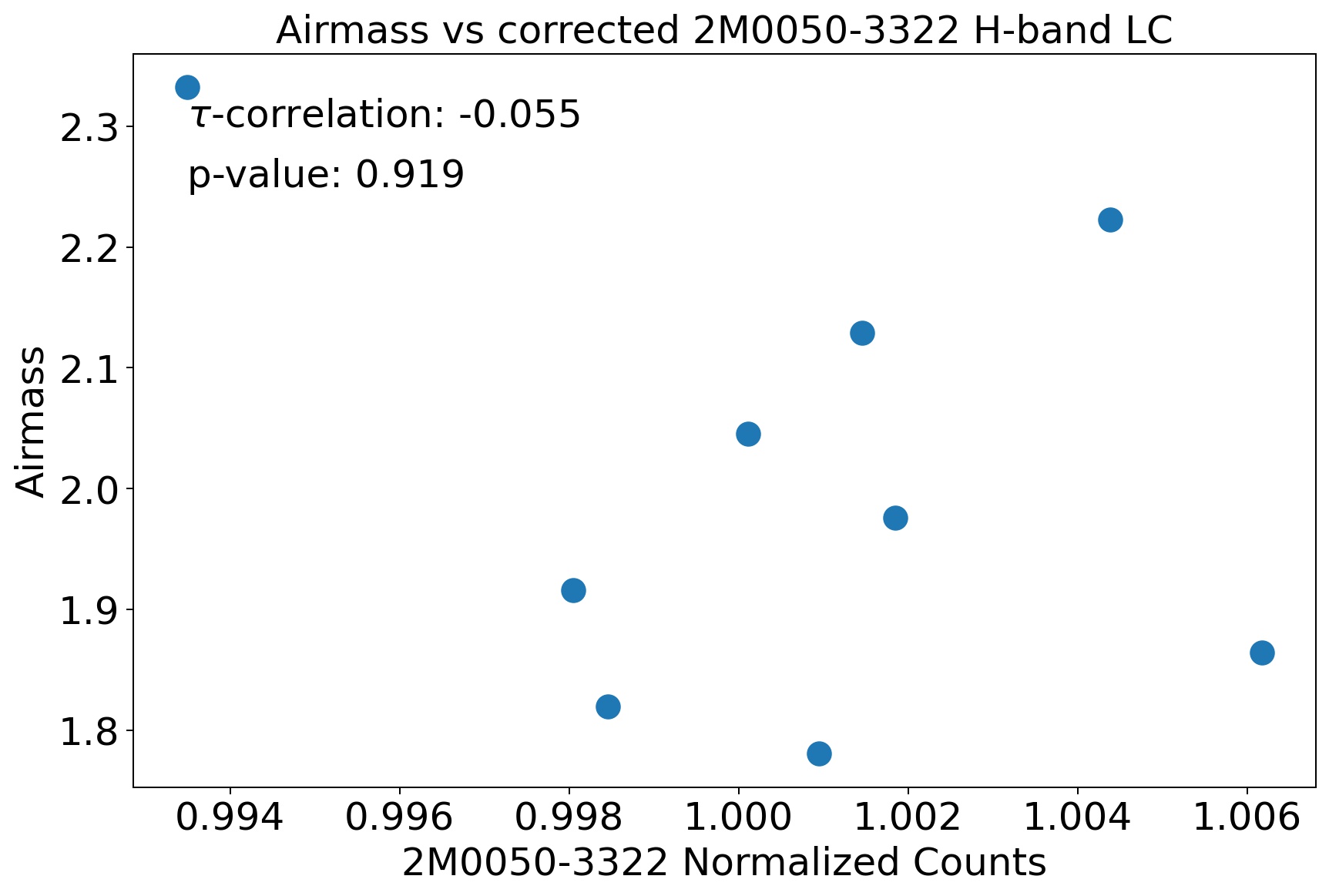
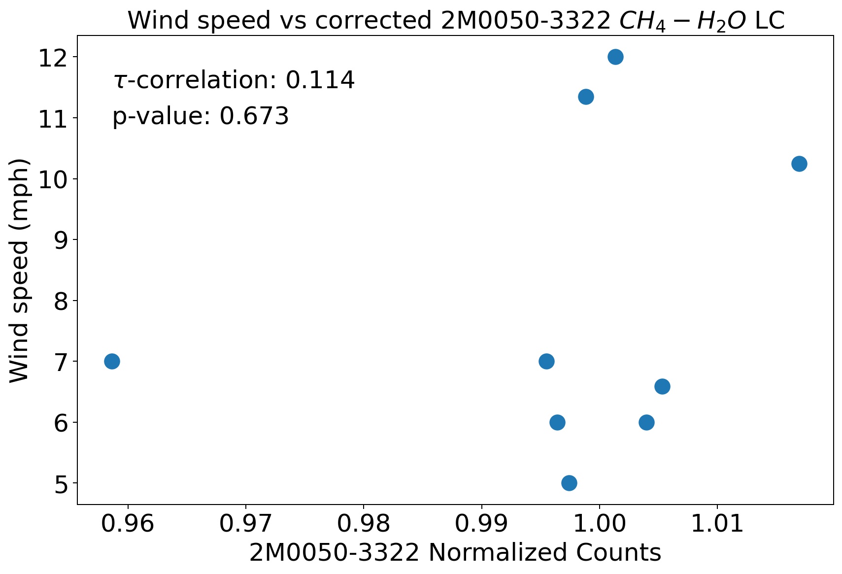
After correcting the $H$-band light curve, we found a moderate correlation with the external temperature ($\tau$ = 0.44, p-value = 0.12), and a weak anticorrelation with the humidity content ($\tau$ = -0.20, p-value = 0.46), and the seeing ($\tau$ = -0.16, p-value = 0.61). A weak correlation with the wind speed ($\tau$ = 0.11, p-value = 0.67), and a no correlation with the airmass ($\tau$ = -0.06, p-value = 0.92). The plots showing all correlations can be found in Fig. 29 in the Appendix.

6.3.3 $\mathrm{CH_{2}-H_{2}O}$ light curves

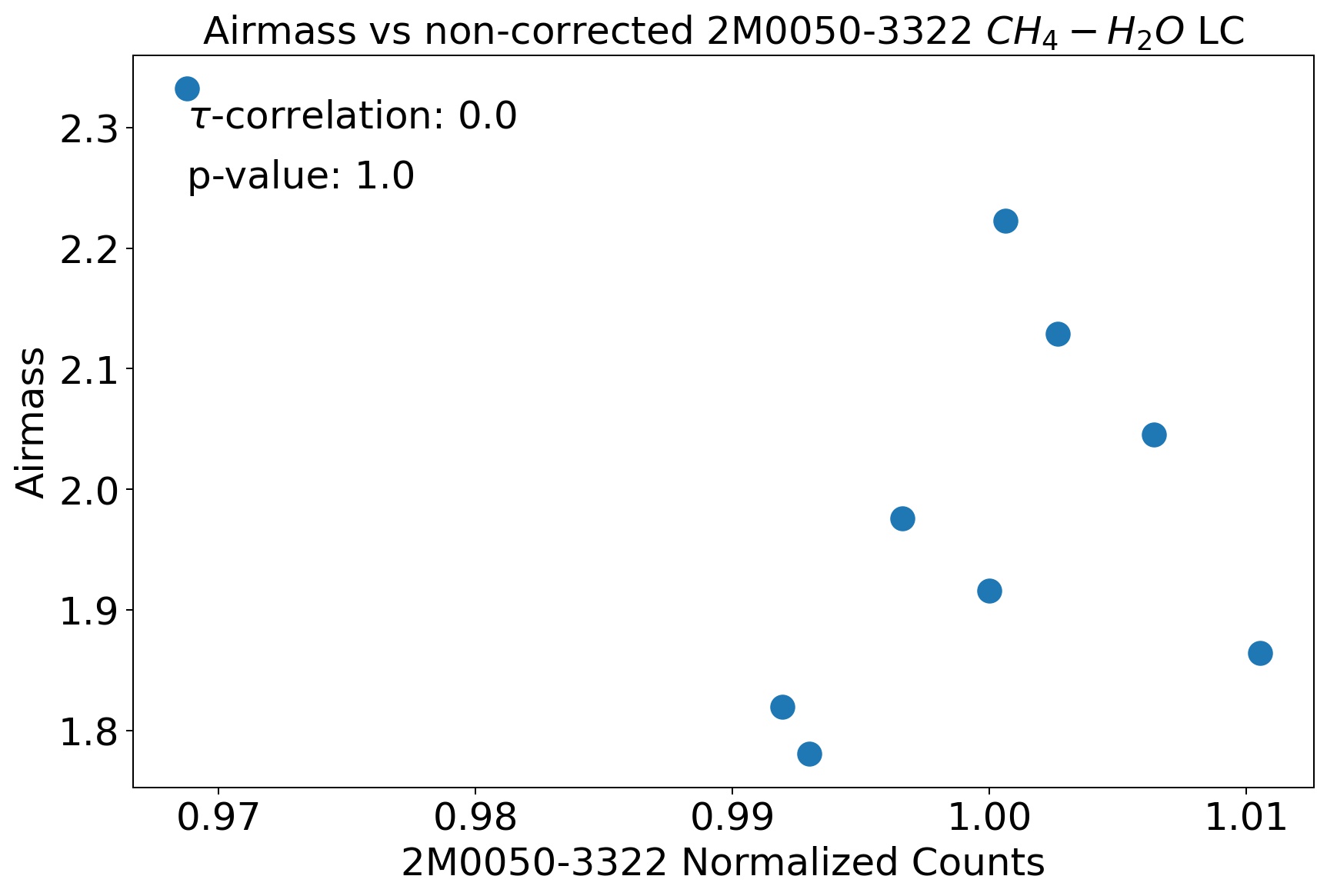
We calculated the $\tau$ Kendall correlation coefficient between the non-corrected, and corrected $\mathrm{CH_{2}-H_{2}O}$ spectrophotometric light curves for 2M0050–3322, and each of the atmospheric parameters mentioned above. We found no correlation between the airmass and the non-corrected $\mathrm{CH_{2}-H_{2}O}$ light curve of 2M0050–3322 ($\tau$ = 0.0, p-value = 1.0), a no correlation with the humidity content ($\tau$ = 0.08, p-value = 0.75), and the seeing ($\tau$ = 0.0, p-value = 1.0). We measure a weak correlation with the wind speed ($\tau$ = -0.11, p-value = 0.67), and the external temperature ($\tau$ = -0.39, p-value = 0.18). The correlation plots can be found in Fig. 30 of the Appendix.

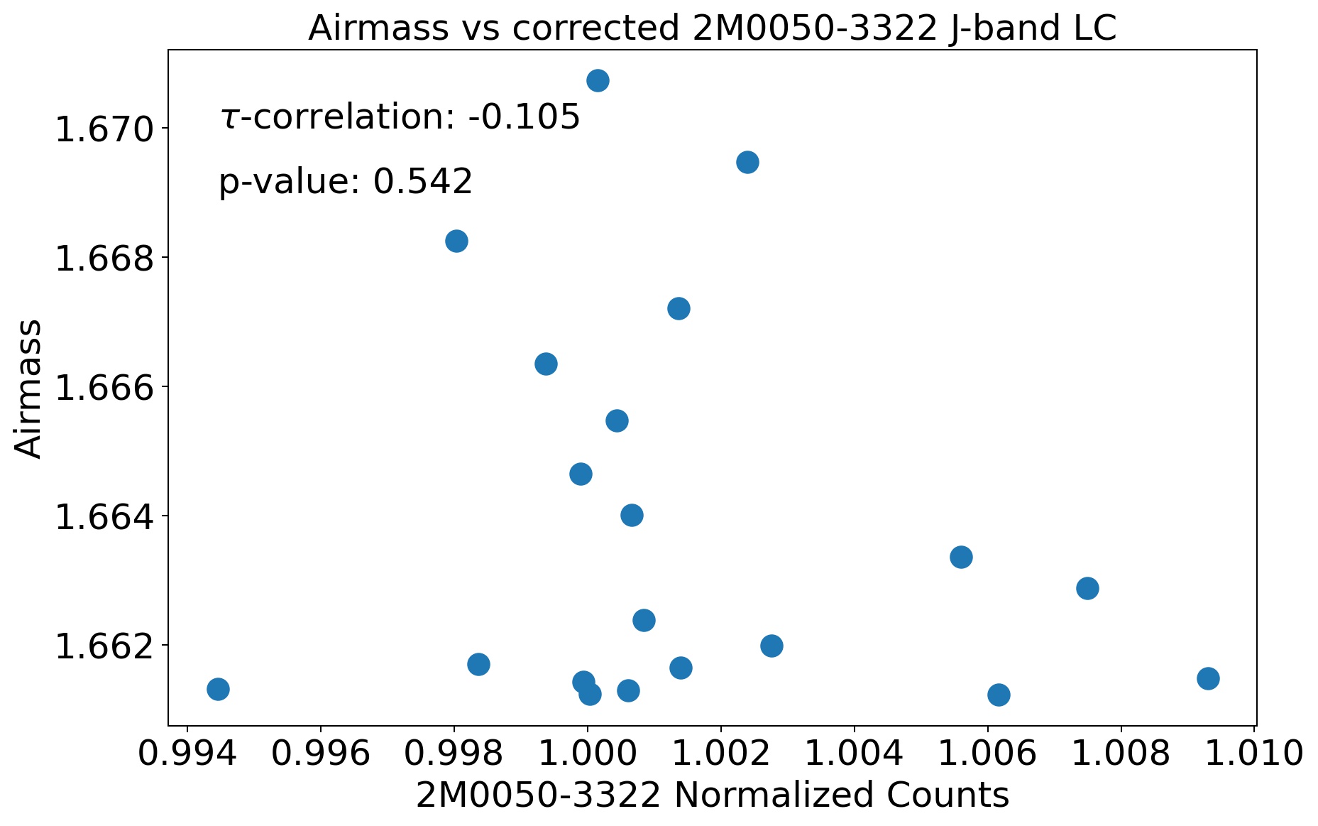
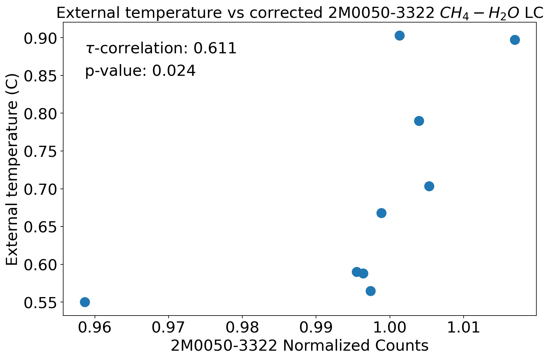
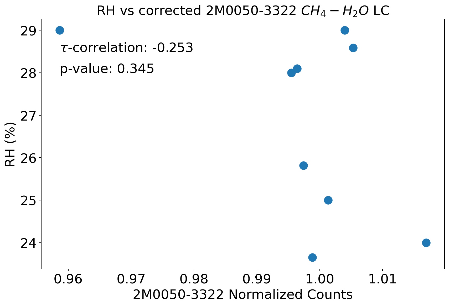
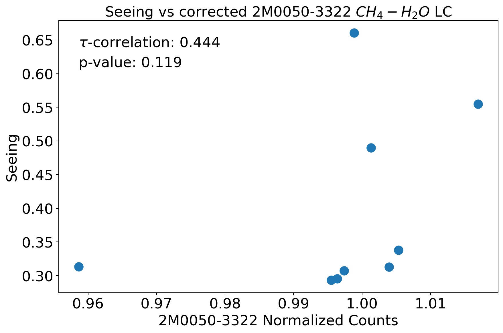
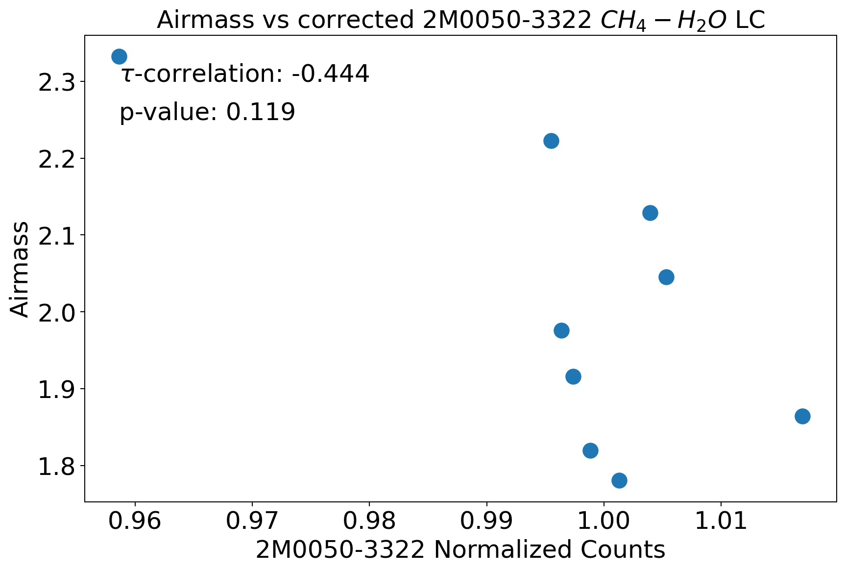
After correcting the $\mathrm{CH_{2}-H_{2}O}$ light curve, we found a moderate correlation with the external temperature ($\tau$ = 0.61, p-value = 0.02), and the seeing ($\tau$ = 0.44, p-value = 0.12), and a moderate anticorrelation with airmass ($\tau$ = -0.44, p-value = 0.12). We find a weak anticorrelation with the humidity content ($\tau$ = -0.25, p-value = 0.35), and a weak correlation with the wind speed ($\tau$ = 0.11, p-value = 0.67). The plots showing all correlations can be found in Fig. 31 in the Appendix.

6.4 Differential Chromatic Refraction

The differential chromatic refraction (DCR) produces an astrometric shift in the position of a source when observed at high airmasses with respect the same source observed at low airmasses, because of the dependence of the refractive index of the air with wavelength (Filippenko, 1982). The DCR effect is higher at higher airmasses, and at shorter wavelengths, being very relevant in the blue optical. The DCR also depends on the external temperature, atmospheric pressure and the spectral type (colors) of the astronomical sources (Stone, 1996).

A shift in the position of the spectra in the MOSFIRE detector could cause spurious flux changes due to pixel-to-pixel variation effects. Since our observations were performed at high airmasses, between 1.79 and 2.37, we investigate the magnitude that this effect might have in our spectro-photometric measurements in the $H$-band. We used the equation in Stone (1996) to estimate the magnitude of the DCR effect in a maximum of $\sim$10 mas, which is about 1/20 of a MOSFIRE pixel (MOSFIRE scale plate of 0.1798”/pix). Given that 2M0050–3322 does not have very distinct colors from the rest of the calibration stars in the field (see Table 8), we expect the effect to affect all sources similarly.

Table 8: 2MASS $J$, $H$, and $K$ magnitudes and $J-H$, $J-K$ and $H-K$ colors for 2M0050–3322 and calibration stars.

	$J$	e$J$	$H$	e$H$	$K$	e$K$	$J-H$	e$J-H$	$J-K$	e$J-K$	$H-K$	e$H-K$
2M0050—3322	15.928	0.070	15.828	0.191	15.241	0.185	0.100	0.203	0.687	0.198	0.587	0.266
Star 1	15.642	0.062	15.274	0.113	14.892	0.150	0.368	0.129	0.750	0.162	0.382	0.188
Star 2	14.926	0.047	14.475	0.057	14.310	0.088	0.451	0.074	0.616	0.100	0.165	0.105
Star 3	16.561	0.160	15.905	0.207	15.891	0.336	0.656	0.262	0.670	0.372	0.014	0.395
Star 5	16.146	0.098	15.524	0.152	15.178		0.622	0.181	0.968	0.098	0.346	0.152

7 Results

7.1 Photometric fluctuations

The total time of $J$- and $H$-band monitoring is $\sim$2.6 hr, with a gap of $\sim$25 min between the $J$-band imaging and spectroscopic data. We observed $\sim$0.45 hr in $J$-imaging mode, $\sim$0.35 hr in $J$-band spectrophotometric mode, and 1.4 hr in $H$-band spectrophotometric mode, covering almost two rotational periods of 2M0050–3322 (P = 1.55$\pm$0.02 hr, Metchev et al. 2015). As mentioned above, the three corrected light curves are shown in Fig. 7. We measured a peak-to-peak (maximum to minimum) amplitude on their fluctuations of 1.48$\pm$0.75% for the $J$-band imaging light curve, 0.62$\pm$0.18% $J$-band spectrophotometric light curve, and a 1.26$\pm$0.93% for the $H$-band spectrophotometric light curve. The $CH_{4}-H_{2}O$ light curve shows relatively higher amplitude of 5.33$\pm$2.02% (see Fig. 6, right).

7.1.1 BIC Test for Significant Variability

To test the significance of the observed fluctuations in the light curve of 2M0050–3322, we used the Bayesian Information Criterion (BIC) as in Manjavacas et al. (2021), Vos et al. (2020) and Naud et al. (2017). The BIC is defined as:

$$\mathrm{BIC}=-2~{}\mathrm{ln}~{}\mathcal{L}_{\mathrm{max}}+k~{}\mathrm{ln}~{}N$$ (1)

where $\mathcal{L}_{\mathrm{max}}$ is the maximum likelihood achievable by the model. The likelihood function, $\mathcal{L}$, is given by

$$\mathcal{L}=\prod_{i=1}^{n}\frac{1}{\sqrt{2\pi s^{2}}}e^{\frac{-(y_{i}-f(\theta))^{2}}{2s^{2}}}$$ (2)

where $s$ is the flux uncertainty, $y_{i}$ is the measured flux, $f(\theta)$ is the model flux. $\mathcal{L}_{\mathrm{max}}$ is obtained by maximizing this function. $k$ is the number of parameters in the model. The flat model has one parameter – the constant relative flux value. The sinusoidal model has four parameters – the constant flux value as well as the amplitude, period and phase. The BIC thus penalizes the sinusoidal model for having additional parameters compared with the flat model. $N$ is the number of data points used in the fit. $\Delta\mathrm{BIC}>0$ indicates that the sinusoidal model is favored and $\Delta\mathrm{BIC}<0$ indicates that the non-variable, flat model is favored. A $|\Delta\mathrm{BIC}|$ value between 0 and 6 indicates that one model is positively favored over the other, a value between 6 and 10 indicates that one model is strongly favored over the other and values above 10 indicate that one model is very strongly favored over the other (Schwarz, 1978).

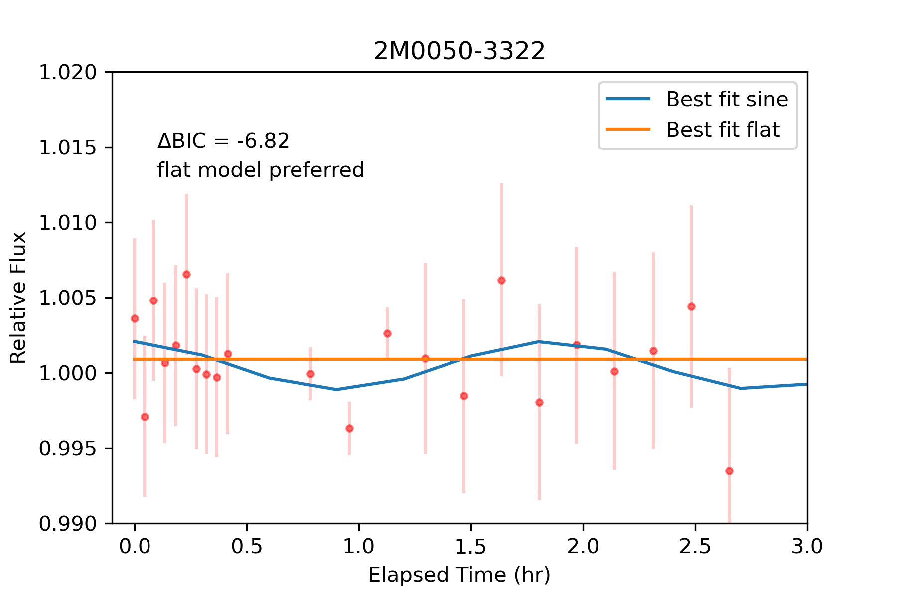
We calculate $\Delta\mathrm{BIC}=\mathrm{BIC}_{flat}-\mathrm{BIC}_{\mathrm{sin}}$ to assess whether a variable sinusoidal or non-variable flat model is favored by the data. The sinusoidal and flat model are shown in Fig. 8. We obtained a $\Delta\mathrm{BIC}$ value of -6.82, that implies that the flat model is strongly preferred over a sinusoidal model. A similar result was obtained if we run the BIC test on the individual $J$, $H$-band and $CH_{4}-H_{2}O$ light curves. The fact that the fluctuation of the $CH_{4}-H_{2}O$ light curve are higher than for the $J$- and $H$-band light curves, is due to the last point of the $CH_{4}-H_{2}O$ light curve having a lower flux than the rest, which explains why the BIC test still finds no significant variability.

Figure 8: 2M0050–3322 light curve is shown by the orange points, with the best-fit non-variable (flat) model shown in orange, and variable (sinusoidal) model shown in blue. The BIC test shows that the flat model is strongly favored by the light curve.

To understand which conditions the 2M0050–3322 light curve should meet so that the BIC analysis favors the sinusoidal model versus the flat model, we artificially modified the 2M0050-3322 light curve by changing the uncertainties of each point (brighter target). To obtain a statistically significant result, we use a Monte Carlo simulation to produce synthetic light curves similar to 2M0050–3322 light curve. We generated 100 synthetic light curves using the original light curve redefining each data point using a Gaussian random number generator. The mean of the Gaussian is the measured flux of the original light curve, and the standard deviation is the photometric uncertainty of each point in the light curve, but divided by a factor. These factors are 1 (similar light curve to the original one), 2, 3 and 4. We generate 100 light curves with each factor used to reduce the uncertainties of the light curve. Then we carry the BIC analysis again, and find which conditions the light curve must meet to be considered significantly variable. For the light curves generated using the uncertainties of the original 2M0050 light curve, we found that  48% of the times the light curve was flagged as variable, and  52% as non-variable. For the light curves generated using the uncertainties divided by 2, we found that  2% of the light curves are significantly variable, and  98% non-variable. For the light curves generated with the uncertainties of 2M0050 divided by 3, and by 4, we found that none of the light curves was found significantly variable.

7.1.2 MOSFIRE sensitivity

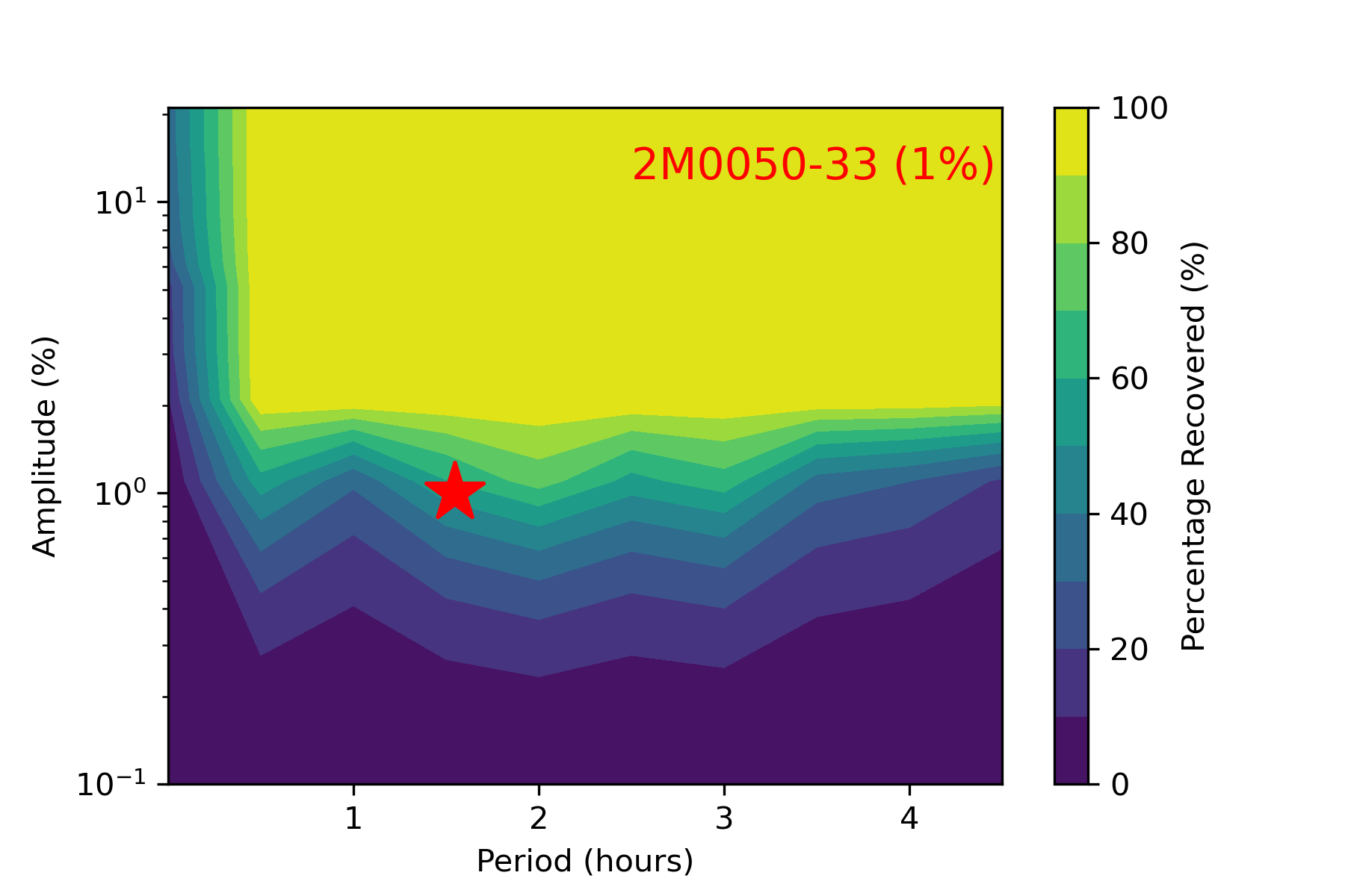
We estimated the sensitivity of MOSFIRE to detect a light curve with a significant variability amplitude, and with a similar amplitude to the fluctuations of the 2M0050–3322 light curve ($\sim$1%). This test allow us to determine the upper limit of the variability amplitude detectable with MOSFIRE. To create the sensitivity plot, we followed the same approach as for Vos et al. (2020, 2022), injecting sinusoidal curves into artificial light curves created using a Gaussian-distributed noise. Simulated amplitudes were in the range $0.01-22\%$ in steps of 1% and period were in the range $0.001-5~{}$hr in steps of $0.5~{}$hr. We also simulated 1000 random phases for each set of (A,P) paramters, resulting in a total of 220,000 simualted light curves. Then, using a Lomb-Scargle periodogram, we estimated the probability of detection as the percentage of light curves with a given variability amplitude and period that produce a periodogram power above a given threshold (1% false-alarm probability). We show the sensitivity plot in Fig. 9. We placed a red star in Figure 9 for the peak-to-peak amplitudes of the fluctuations measured for the $J$- and $H$-band light curves with a rotational period of 1.55$\pm$0.02 hr (Metchev et al., 2015).

The sensitivity plot concludes that MOSFIRE would be able to detect a 1.0% variability amplitude light curve between 50–60% of the times. Thus, given the sensitivity of MOSFIRE with the observation strategy followed in this work, we might not be able to detect significant variability in 40–50% of the cases. MOSFIRE would be able to detect between 90–100% of the cases a light curve with a minimum variability amplitude of 2% for an object with a similar magnitude to 2M0050–3322.

Figure 9: Sensitivity plot for Keck 1/MOSFIRE. MOSFIRE would be able to measure the predicted light curve for a T7.0 brown dwarf similar to 2M0050–3322 50-60% of the times with the observation strategy followed in this work.

7.2 Spectral fluctuations

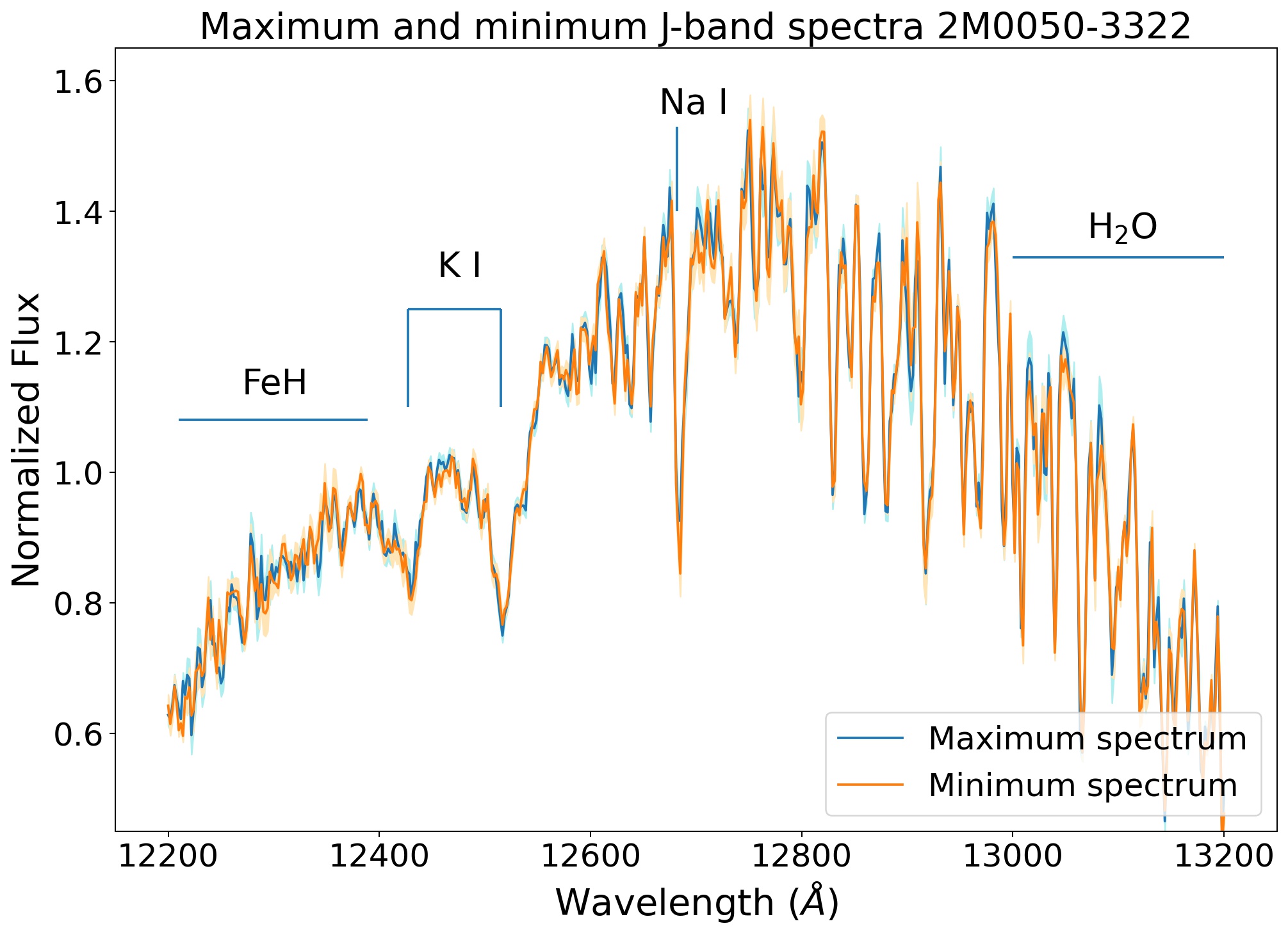
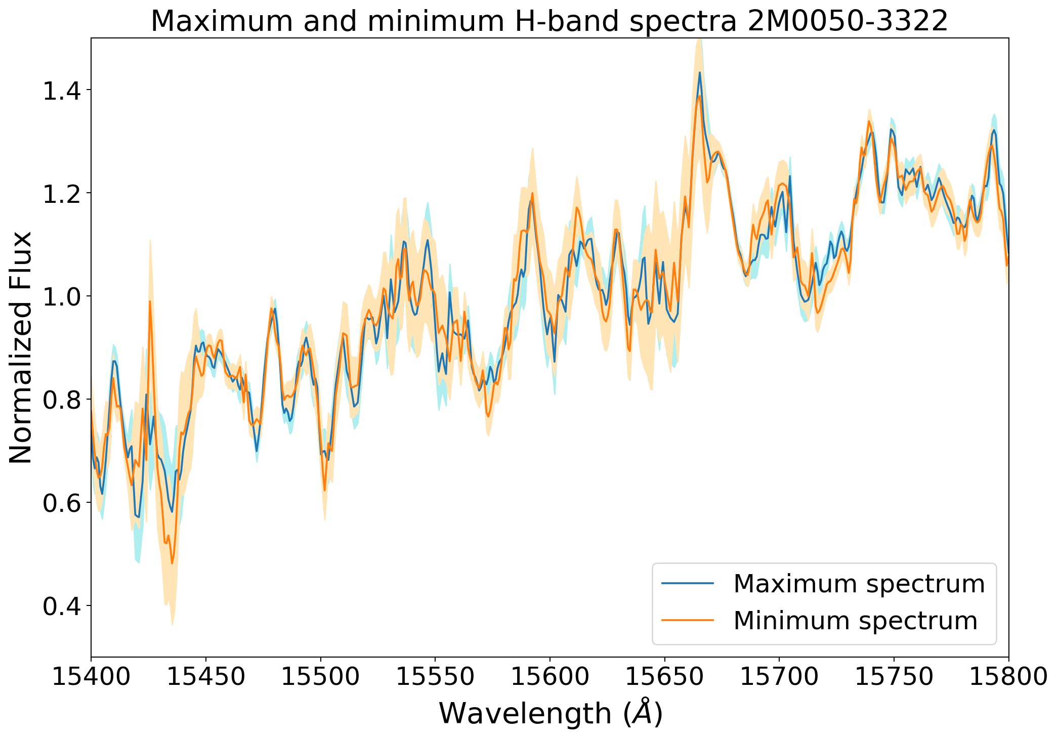
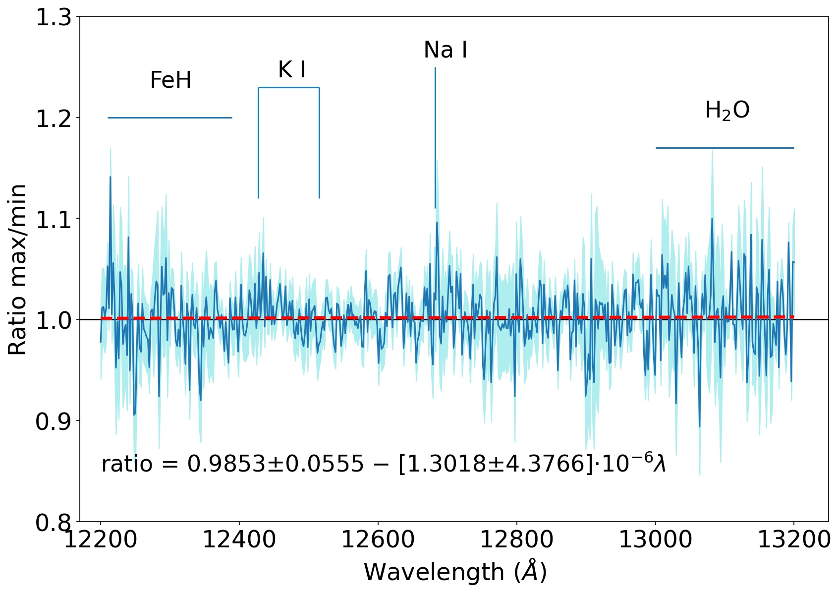
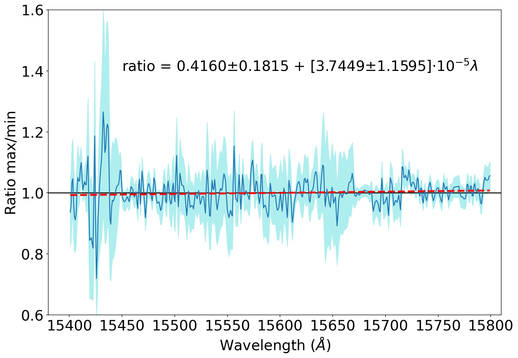
Given that we did not detect significant variability for 2M0050–3322 in Section 7.1, the spectral peak-to-peak fluctuations measured, and its wavelength dependence presented in this section are only tentative. We measured the peak-to-peak fluctuations dependence as a function of wavelength by dividing the maximum and minimum flux spectra in the $J$ and $H$-band spectrophotometric data. In Fig. 10 we show the maximum and minimum flux spectra for both filters. In Fig. 11 we show the ratio of those spectra in the $J$ and $H$-band, i.e. the relative peak-to-peak fluctuations across the wavelength range of those bands with their uncertainties, indicating the molecular and atomic absorption features of 2M0050–3322. We fit a line to the ratio of the maximum and minimum flux spectra using the numpy.polyfit Python library to the $J$ and $H$-band ratio independently. We obtained a slope consistent with zero for the $J$-band ratio ($ratio=0.9853\pm 0.0555--[1.3018\pm 4.3766]\times 10^{-6}\lambda$, see Fig. 11, left), and a tentative positive slope (3-$\sigma$) to the $H$-band ratio ($ratio=0.4160\pm 0.1815+[3.7449\pm 1.1595]\times 10^{-5}\lambda$, see Fig. 11, right), suggesting that the peak-to-peak fluctuations might increase slightly from 15400 to 15800 $\AA$. Within the 15400 to 15800 $\AA$ wavelength range the values of the ratio are consistent within the uncertainties. The value of the ratio at 15400 $\AA$ is 0.9927$\pm$0.2547 and 1.0077$\pm$0.2579 at 15800 $\AA$. Thus, we cannot measure a significant ratio increase within this wavelength range, although the slope of the $H$-band ratio is significantly positive.

Figure 10: Left: Maximum flux $J$-band spectrum for 2M0050-332 (orange), and minimum $J$-band spectrum for 2M0050-332 (blue). Right: Maximum flux $H$-band spectrum for 2M0050-332 (orange), and minimum $H$-band spectrum for 2M0050–3322 (blue).

Figure 11: Left: Ratio of the maximum divided by the minimum spectra of 2M0050–3322 in the $J$-band. Right: Ratio of the maximum divided by the minimum spectra of 2M0050–3322 in the $H$-band.

8 Discussion

The 2M0055–3322 $J$-band imaging light curve shows fluctuations with a peak-to-peak amplitude of 1.48$\pm$0.75%. The $J$-band spectroscopic light curve shows fluctuations with a peak-to-peak amplitude of 0.62$\pm$0.18% (with just three data points). The $H$-band spectrophotometric light curve has fluctuations with peak-to-peak amplitude of 1.26$\pm$0.93%, compatible with the amplitude derived for the $J$-band imaging and spectrophotometric light curves (Fig. 7). Finally, the fluctuation of the $\mathrm{CH_{4}-H_{2}O}$ light curve is 5.33$\pm$2.02%. Radigan et al. (2014) did not detect significant variability in their imaging $J$-band light curve for 2M0050–3322, but provided an upper limit of 1.1% peak-to-peak amplitude, with the WIRC camera in the Du Pont telescope in Las Campanas observatory, which is a 2.5 m telescope. Metchev et al. (2015) measured a variability amplitude of $<$0.59% for the [3.6] Spitzer channel light curve, and an amplitude of 1.07$\pm$0.11% in the [4.5] Spitzer channel light curve. The last value is consistent with the amplitudes measured for the $J$-band and $H$-band light curves, even though these bands trace deeper layers of the atmosphere of 2M0050–3322 than the Spitzer mid-infrared channels (Yang et al., 2016), and the observations were separated in time by several years.

The BIC analysis presented in Section 7.1.1 favors the flat light curve model versus a sinusoidal model, indicating that the peak-to-peak fluctuations measured in the 2M0050–3322 light curve might suggest in the best case tentative low-level variability.

Few mid and late-T dwarfs have been monitored for variability at all. For completeness we include a list of all mid and late-T dwarfs with upper limits or measurements of variability (see Table 9). Furthermore, only two other late-T dwarfs have been monitored for spectro-photometric variability: 2MASS J22282889–431026 (T6.5, Buenzli et al. 2012), and Ross 458c (T7.5, Manjavacas et al. 2019), both with HST/WFC3 and its G141 grism. Comparing the light curves of these two late-T brown dwarfs, their variability amplitudes, and wavelength variability dependence we find several differences and commonalities between them. 2MASS J22282889–431026 (2M2228-4310) and Ross 458c have sinusoidal light curves (from Buenzli et al. 2012 and Manjavacas et al. 2019, respectively). Their $J$-band variability amplitude is smaller than the $H$-band (1.85$\pm$0.07% vs 2.74$\pm$0.11% for 2M2228-4310, and 2.62$\pm$0.02% vs 3.16$\pm$1.26% for Ross 458c). The rotational period of 2M2228-4310 is shorter (1.41$\pm$0.01 hr, Buenzli et al. 2012) than for Ross 458c (6.75$\pm$1.58 hr, Manjavacas et al. 2019). Ross 458c shows a dependence of its variability amplitude with wavelength, but only in the $J$-band. 2M2228-4310 does not show any wavelength dependence in the $J$ or $H$-bands. Both 2M2228-4310 and Ross 458c show phase shifts between the $J$- and $H$-band light curves, and with the $\mathrm{CH_{4}-H_{2}O}$ light curve. With the MOSFIRE $J$- $H$- and $\mathrm{CH_{4}-H_{2}O}$ light curves presented here, we were not able to confirm or discard if the shape of 2M0050–3322 light curve is also sinusoidal. We could not confirm the rotational period of 1.55$\pm$0.02 hr measured by Metchev et al. (2015), and we could not confirm nor rule out phase shifts between the $J$- and $H$-band light curves 2M0050–3322. The peak-to-peak amplitudes of the fluctuations measured in the $J$- and $H$-band, and $\mathrm{CH_{4}-H_{2}O}$ 2M0050–3322 light curves are smaller than the amplitudes measured for 2M2228-431 and Ross 458c. A higher sample of mid to late-T dwarfs with photometric or spectro-photometric variability information would help to confirm similarities between the light curves of mid to late-T dwarfs, and further investigate and explain their differences.

Table 9: List of T-dwarfs with spectral type $>$T5.0 with upper levels or measurements of photometric or spectro-photometric variability up-to-date.

Name	RA	DE	SpT	A ($J$-band)	A ($H$-band)	A([3.6])	A([4.5])	Period	Ref.
			(NIR)	(%)	(%)	(%)	(%)	(hr)
J034807–602227	03 48 07.72	-60 22 27.00	T7.0	…	…	…	1.5$\pm$1.4	1.080$\pm$1.075	(9)
J005019–332240	00 50 19.94	-33 22 40.27	T7.0	$<0.7\pm 0.4$	…	<0.59	$1.07\pm 0.11$	$1.55\pm 0.02$	(2)(4)
J024313–245329	02 43 13.71	-24 53 29.83	T6.0	$0.040\pm 0.011$		…	…	…	(4)(6)
J051609–044549	05 16 09.45	-04 45 49.93	T5.5	…	…	<0.83	<0.81	…	(2)
J081730–615520	08 17 29.99	-61 55 15.65	T6.0	$\sim$0.6	$1.93\pm 0.005$	…	…	$2.8$	(4)(7)
J104753+21242	10 47 53.85	+21 24 23.46	T6.5	…	…	…	0.5	$1.741\pm 0.007$	(8)
Ross 458c	13 00 42.08	+12 21 15.05	T8.5	$2.62\pm 0.02$	…	<1.37	<0.72	$6.75\pm 1.58$	(2)(3)
J141623+134836	14 16 23.94	+13 48 36.32	T7.5	…	…	<0.91	<0.59	…	(2)
J154627–332511	15 46 27.18	-33 25 11.18	T5.5	$0.014\pm 0.008$		…	…	…	(5)(4)
J182835–484904	18 28 35.72	-48 49 04.63	T5.5	$0.9\pm 0.1$		…	…	$5.0\pm 0.6$	(5)(6)
J222828–431026	22 28 28.89	-43 10 26.27	T6.5	$1.85\pm 0.07$	$2.74\pm 0.11$	$4.26\pm 0.2$	$1.51\pm 0.15$	$1.41\pm 0.01$	(1)(2)

Variability references: (1) Buenzli et al. (2012), (2) Metchev et al. (2015), (3) Manjavacas et al. (2019), (4) Radigan et al. (2014) (5) Clarke et al. (2002), (6) Buenzli et al. (2014), (7) Artigau et al. (2009), (8) Allers et al. (2020), (9) Tannock et al. (2021).

9 Interpretation

9.1 Brown Dwarf Storms

The most likely cause of photometric and spectro-photometric variability in brown dwarfs is due to the existence of heterogeneous clouds in their atmospheres (e.g. Apai et al. 2013) that evolve rapidly within few hours. These clouds patterns are not static, and can show beating patterns. Thus, the variability amplitude of brown dwarfs might vary with time (Apai et al., 2017).

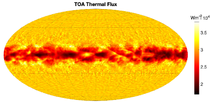
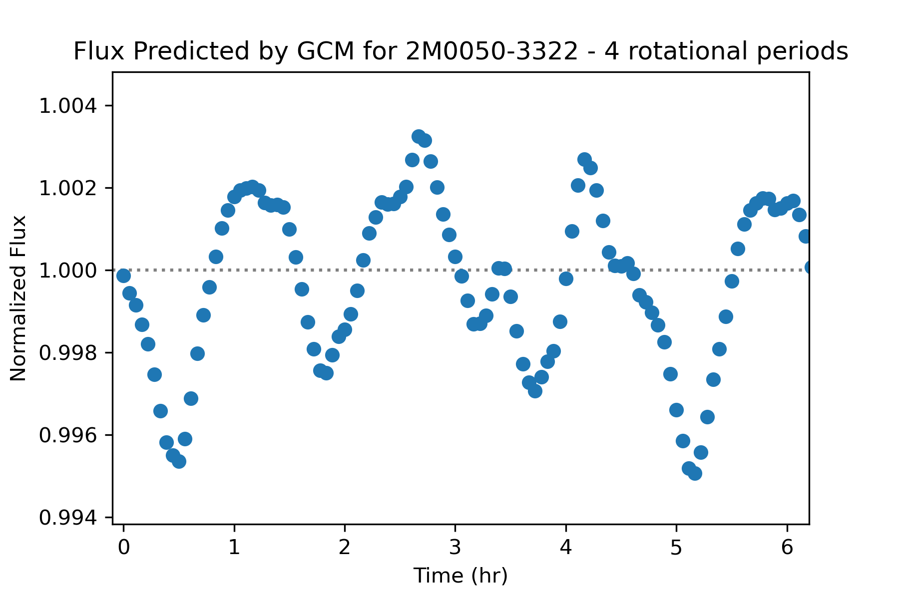
We use General Circulation Models (GCM) developed by Tan & Showman (2021a) to predict the top-of-atmosphere thermal flux for 2M0050-3322. For a T7.0 brown dwarf with log g=5.0, like 2M0050–3322, GCM can provide instantaneous model maps for the top-of-the atmosphere thermal flux, and predict the most likely light curve for such an object. Model details are described in Appendix B. For 2M0050–3322, the vigorous dynamical features and the associated heterogeneous clouds, driven by the radiative feedback of MnS and $\mathrm{Na_{2}S}$ clouds, are expected to be near the equator (see Fig. 12). These equatorial features are large-scale equatorially trapped waves that propagate either eastward or westward relative to mean flow. The GCM predicts a somewhat sinusoidal and regular light curve over a few rotational timescale, with a nearly 1% peak to peak flux variation when the object is viewed equator-on (see Fig. 13). Meanwhile, due to the multiple longitudinal-dependent wave patterns, the light curve also exhibits certain complexities out of a pure sinusoid (see the light curve Figure 13). Vos et al. (2017) found a correlation between close to edge on view, and high variability amplitudes in the $J$-band and in the Spitzer channels because of an increased path length through the atmosphere at low inclination angles. Thus, the GCM provide the variability amplitudes at different inclination angles. For inclinations of 0^∘ (edge on), 30^∘, 60^∘, and 90^∘, the GCM predict variability amplitudes of 1.00%, 0.85%, 0.52% and 0.22%, respectively, in agreement with Vos et al. (2017). Statistics of the dynamical activities in the model, including the characteristic sizes and numbers of storms and cloud thickness, are stable over the long-term model integration. We do not find evidence of sudden decrease or increase of storm activities that could result in dramatic light curve evolution, which is in agreement to light-curve observations for this object in Metchev et al. (2015) and with the peak-to-peak amplitudes of the fluctuations of the light curves presented in this work.

The peak-to-peak variability amplitude predicted by the GCM (Tan & Showman, 2021a) agrees with the peak-to-peak amplitude of the fluctuations measured for the $J$ and $H$-band light curves of 2M0050–3322, even though the variability detected for our target is not significant.

Figure 12: Edge-on map for 2M0050–3322 predicted by General Circulation Models (Tan & Showman, 2021a)

Figure 13: Normalized light curve for an edge-on 2M0050–3322 as predicted by General Circulation Models (Tan & Showman, 2021a). We show four consecutive periods of the light curve.

Similarly, radiative-transfer models with solar-metallicity (Saumon & Marley, 2008) provide the vertical cloud structure expected for the atmosphere of an object with similar effective temperature and surface gravity as 2M0050–3322 ($\mathrm{T_{eff}}$ = 800 K, log g = 5.0, from Filippazzo et al. 2015). Further details on the radiative-transfer models, and how the contribution functions were obtained can be found in Manjavacas et al. (2021), their Section 8.

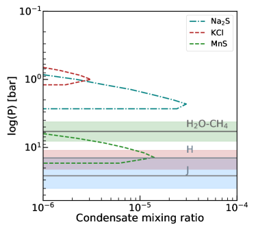
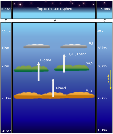
In Fig. 14, we show the predicted condensate mixing ratios by radiative-transfer models (mole fraction) of MnS, KCl and $\mathrm{Na_{2}S}$ clouds for a T7.0 brown dwarf with log g = 5.0. As seen in Fig. 14, at the bottom of the atmosphere, at about $\sim$20 bar, we find the bottom of the MnS cloud. At $\sim$3 bar, we find the bottom of the $\mathrm{Na_{2}S}$ cloud, at $\sim$1.5 bar we find the bottom of the KCl cloud. In Fig. 15 we show a visual representation of the vertical structure of 2M0050–3322, and the pressure levels probed by different near-infrared wavelength ranges. The $J$-band traces the deepest levels, between 20–40 bars, the $H$-band traces the middle levels of the atmosphere, between 10–20 bar, and the $\mathrm{CH_{4}-H_{2}O}$ band traces the medium-upper layers of the atmosphere, around 4–8 bar. Thus, the $J$-band would trace the deepest cloud layers of the atmosphere and above, while the $H$-band would trace the medium layers of the atmosphere, and the $\mathrm{CH_{4}-H_{2}O}$ just the upper layer of the atmosphere. Longer monitoring in time is needed to confirm higher fluctuations in the $\mathrm{CH_{4}-H_{2}O}$ light curve.

Figure 14: Condensate mixing ratio (mole fraction) of MnS, KCl and $\mathrm{Na_{2}S}$ clouds for a T7.0 brown dwarf with log g = 5.0. The mole fraction for each cloud types provide us with the vertical cloud structure of 2M0050–3322.

Figure 15: Visual representation of the different cloud layers in the atmosphere of 2M0050–3322 showing the pressure levels at which each of them condensates, and the top of the atmosphere for reference. We show the traced pressure levels by the different near-infrared wavelengths in our MOSFIRE $J$- and $H$-band spectra.

9.2 Auroral Emission

Until now, the most common mechanism to explain the existence of aurorae in the Giant planets of the Solar System were charged particles from the solar wind that interact with the atmosphere’s particles exiting them, and producing an emission (Clarke, 2013). Nevertheless, Saturn has been recently found to have aurorae also connected to storms or vortexes in its atmosphere (in the polar region) or weather-driven aurorae (Chowdhury et al., 2022). Chowdhury et al. (2022) used spectral observations of auroral $H_{3}^{+}$ emission lines in near-infrared high resolution data, a dominant molecular ion species in Saturn’s ionosphere, to trace the electrical dynamo region of the ionosphere. Using the $H_{3}^{+}$ emission lines Chowdhury et al. (2022) detected twin-vortex flows in the upper atmosphere of Saturn, consistent with theories that predict the presence of such a polar feature. This is the first time that a connection between aurorae and weather patterns have been observed in a Solar System giant planet, with the subsequent implications for cold brown dwarfs, where weather is the most likely explanation for potential aurorae.

A handful of brown dwarfs have been found to have radio emissions potentially connected to the existence of aurorae. The first one was LSRJ1835+3259, a M8.5 brown dwarf at the lithium-burning boundary, for which radio and optical auroral emission were detected (Hallinan et al., 2015). Since then, radio emissions have been found in other brown dwarfs, some of them rapid rotating late T-dwarfs like 2M0050–3322. This is the case of WISEPC J112254.73+255021.5 (T6.0), that shows radio emissions with a period of 0.28 hr (Route & Wolszczan, 2016), and 2MASS J10475385+2124234 (T6.5), with a periodic emission of 1.741$\pm$0.007 hr (Allers et al., 2020) suggesting the existence of aurorae in both objects. 2M0050–3322 shares a similar spectral type (T7.0) and rapid rotational period of 1.55$\pm$0.02 hr as measured by Metchev et al. (2015). No radio emission has been searched for 2M0050–3322, but aurorae could potentially have an influence in the fluctuations measured in the $J$-, $H$-bands, and the $\mathrm{CH_{4}-H_{2}O}$ band, as recently found for Saturn (Chowdhury et al., 2022).

10 Conclusions

1. We have used MOSFIRE at the Keck I telescope to monitor 2MASS J00501994–3322402, a field (0.5–10 Myr) T7.0 brown dwarf over $\sim$2.6 hr in the $J$- and $H$-bands.

2. We measured peak-to-peak fluctuations of 1.48$\pm$0.75% in the $J$-band imaging light curve, 0.62$\pm$0.18% in the $J$-band spectrophotometric light curve, a 1.26$\pm$0.93% in the $H$-band, and a 5.33$\pm$2.02% in the $\mathrm{CH_{4}-H_{2}O}$ band. The $J$- and $H$-band peak-to-peak fluctuation amplitudes agree with those measured by Metchev et al. (2015) in the mid-infrared.

3. The BIC analysis concluded that the 2M0050–3322 $J$-, $H$- and $\mathrm{CH_{4}-H_{2}O}$ band light curves does not show significant variability.

4. We produced a sensitivity plot for our Keck/MOSFIRE observations, concluding that with the current observational strategy we would miss a $\sim$1% variability amplitude light curve in 40-50% of the cases. To detect a significant light curve with MOSFIRE, the variability amplitude of an object similar to 2M0050–3322 should be at least 2%.

5. We tentatively measured the wavelength dependence of the fluctuations in the $J$- and $H$-band light curves. We found no wavelength dependence on the $J$-band fluctuation. In contrast, we measured a tentative slight wavelength dependence in the $H$-band.

6. The peak-to-peak amplitudes of the fluctuations measured for 2M0050–3322 in the $J$- and $H$-bands agree with the predictions of General Circulation Models for a T7.0 brown dwarf with log g = 5.0 (Tan & Showman, 2021a).

7. We show the predicted vertical structure of 2M0050–3322 by radiative-transfer models. At the bottom of the atmosphere ($\sim$20 bar) we find we bottom of the MnS cloud. At $\sim$3 bar, the bottom of the $\mathrm{Na_{2}S}$ cloud, and at $\sim$1.5 bar we find the bottom of the KCl cloud. Given that two of the three clouds used in the radiative-transfer models have the bottom of their cloud between above 4 bar, and that the $\mathrm{CH_{4}-H_{2}O}$ band traces approximately these pressures levels, it might explain why the fluctuations are higher for the $\mathrm{CH_{4}-H_{2}O}$ light curve. Longer monitoring in time is needed to confirm higher fluctuations in the $\mathrm{CH_{4}-H_{2}O}$ light curve.

8. Aurorae probably linked to weather patterns have been discovered for other late-T, fast rotating brown dwarfs similar to 2M0050–3322. Thus the existence of aurorae might contribute to the low-level variability measured for 2M0050–3322.

Appendix A Correlation between parameters

Figure 16: Correlation between the imaging $J$-band target’s non-corrected light curve, and the non-corrected calibration stars light curves.

Figure 17: Correlation between the imaging $J$-band target’s corrected light curve, and the corrected calibration stars light curves.

Figure 18: Correlation between the $H$-band target’s non-corrected light curve, and the non-corrected calibration stars light curves.

Figure 19: Correlation between the $H$-band target’s corrected light curve, and the corrected calibration stars light curves.

Figure 20: Non-corrected (left) and corrected (right) $H$-band light curves of all stars and the target (black line).

Figure 21: Left: Evolution of the calculated FWHM for the $H$-band 2D spectra with time. Right: Evolution of the centroids of the $H$-band 2D spectra with time.

Figure 22: Correlation between the FWHM of the 2D $H$-band spectra and the corrected and non-corrected $H$-band light curve.

Figure 23: Correlation between the centroids of the 2D $H$-band spectra and the non-corrected $H$-band light curve.

Figure 24: Correlation between the $\mathrm{CH_{4}-H_{2}O}$ target’s non-corrected light curve, and the non-corrected calibration stars light curves.

Figure 25: Correlation between the $\mathrm{CH_{4}-H_{2}O}$ target’s corrected light curve, and the corrected calibration stars light curves.

Figure 26: Correlations between the non-corrected $J$-band imaging light curve and different atmospheric parameters.

Figure 27: Correlations between the corrected $J$-band imaging light curve and different atmospheric parameters.

Figure 28: Correlations between the non-corrected $H$-band light curve and different atmospheric parameters.

Figure 29: Correlations between the corrected $H$-band light curve and different atmospheric parameters.

Figure 30: Correlations between the non-corrected $\mathrm{CH_{4}-H_{2}O}$ light curve and different atmospheric parameters.

Figure 31: Correlations between the corrected $\mathrm{CH_{4}-H_{2}O}$ light curve and different atmospheric parameters.

Appendix B The General Circulation Model for the late-T dwarf 2M0050–3322

We use the general circulation model (GCM) originally developed in Tan & Showman (2021b) and Tan & Showman (2021a) to simulate the global three-dimensional temperature, wind and cloud structures for the atmosphere of the late-T brown dwarf 2M0050–3322. The GCM solves the standard dynamical meteorology equations governing the horizontal angular momentum, hydrostatic balance, mass continuity, thermodynamics and equation of state. A set of tracer equations are solved simultaneously for the dynamical transport of the condensable vapor and cloud components of the atmosphere. A grey (wavelength averaged), two-stream radiative transfer scheme is used to solve for the thermal radiation. The opacity sources include the Rosseland-mean gas opacity of solar metallicity obtained from Freedman et al. (2014), and the absorption and scattering due to localtion- and time-dependent cloud particles. The strong radiative heating/cooling rates due to inhomogeneous cloud structures drive the general circulation, which in turn maintains the large-scale patchy cloud configuration.

A similar set of GCMs for brown dwarfs Luhman A and B is performed in Mukherjee et al. (2021) in which the major cloud species was assumed to be ${\rm MgSiO_{3}}$, appropriate for those L/T transition dwarfs. The GCM in this study differs to those used in Mukherjee et al. (2021) in that the major cloud species here are ${\rm MnS}$ and ${\rm Na_{2}S}$ which are the two most representative species near the photospheres of late-T dwarfs (e.g., Morley et al., 2012, see also Figure 14). The temperature-pressure-dependent condensation curves of ${\rm MnS}$ and ${\rm Na_{2}S}$ at solar metallicity are given by Visscher et al. (2006). More details of the cloud scheme are referred to Tan & Showman (2021b, a) and Mukherjee et al. (2021). We assume a fixed cloud particle number per dry air mass $N_{c}=10^{-9}\;{\rm kg^{-1}}$ throughout the atmosphere. When clouds form, the characteristic particle size is determined by the amount of local cloud mass mixing ratio and $N_{c}$. For solar abundance of condensable gases, clouds particles are sub-micron in our model.

The GCM uses a horizontal resolution equivalent to 256 and 512 grid points in the latitudinal and longitudinal directions. There are 45 vertical layers in the model, which are evenly discretized in the log-pressure space in between 0.005 bar and 100 bars. A relatively weak frictional drag with a drag timescale of $10^{7}$ s is applied at deep layers with pressures larger than 50 bars, representing angular momentum mixing between the modeled layer and the deep interior. The model has been integrated over 1200 Earth days and has reached statistical equilibrium.

References

- Allers et al. (2020) Allers, K. N., Vos, J. M., Biller, B. A., & Williams, P. K. 2020, Science, 368, 169
- Allers et al. (2020) Allers, K. N., Vos, J. M., Biller, B. A., & Williams, P. K. G. 2020, Science, 368, 169, doi: 10.1126/science.aaz2856
- Apai et al. (2013) Apai, D., Radigan, J., Buenzli, E., et al. 2013, ApJ, 768, 121, doi: 10.1088/0004-637X/768/2/121
- Apai et al. (2017) Apai, D., Karalidi, T., Marley, M. S., et al. 2017, Science, 357, 683, doi: 10.1126/science.aam9848
- Artigau et al. (2009) Artigau, É., Bouchard, S., Doyon, R., & Lafrenière, D. 2009, ApJ, 701, 1534, doi: 10.1088/0004-637X/701/2/1534
- Astropy Collaboration et al. (2013) Astropy Collaboration, Robitaille, T. P., Tollerud, E. J., et al. 2013, A&A, 558, A33, doi: 10.1051/0004-6361/201322068
- Bailer-Jones & Mundt (1999) Bailer-Jones, C. A. L., & Mundt, R. 1999, A&A, 348, 800. https://arxiv.org/abs/astro-ph/9906439
- Biller et al. (2018) Biller, B. A., Vos, J., Buenzli, E., et al. 2018, AJ, 155, 95, doi: 10.3847/1538-3881/aaa5a6
- Buenzli et al. (2014) Buenzli, E., Apai, D., Radigan, J., Reid, I. N., & Flateau, D. 2014, ApJ, 782, 77, doi: 10.1088/0004-637X/782/2/77
- Buenzli et al. (2012) Buenzli, E., Apai, D., Morley, C. V., et al. 2012, ApJ, 760, L31, doi: 10.1088/2041-8205/760/2/L31
- Burgasser et al. (2006) Burgasser, A. J., Geballe, T. R., Leggett, S. K., Kirkpatrick, J. D., & Golimowski, D. A. 2006, ApJ, 637, 1067, doi: 10.1086/498563
- Caballero et al. (2004) Caballero, J. A., Béjar, V. J. S., Rebolo, R., & Zapatero Osorio, M. R. 2004, A&A, 424, 857, doi: 10.1051/0004-6361:20047048
- Chowdhury et al. (2022) Chowdhury, M. N., Stallard, T. S., Baines, K. H., et al. 2022, Geophysical Research Letters, 49, doi: 10.1029/2021gl096492
- Clarke et al. (2002) Clarke, F. J., Oppenheimer, B. R., & Tinney, C. G. 2002, MNRAS, 335, 1158, doi: 10.1046/j.1365-8711.2002.05691.x
- Clarke (2013) Clarke, J. T. 2013, in Geophysical Monograph Series (American Geophysical Union), 113–122, doi: 10.1029/2011gm001199
- Croux & Dehon (2010) Croux, C., & Dehon, C. 2010, Statistical Methods & Applications, 19, 497, doi: 10.1007/s10260-010-0142-z
- Cutri et al. (2003) Cutri, R. M., Skrutskie, M. F., van Dyk, S., et al. 2003, VizieR Online Data Catalog, 2246, 0
- Dupuy & Liu (2012) Dupuy, T. J., & Liu, M. C. 2012, ApJS, 201, 19, doi: 10.1088/0067-0049/201/2/19
- Filippazzo et al. (2015) Filippazzo, J. C., Rice, E. L., Faherty, J., et al. 2015, ApJ, 810, 158, doi: 10.1088/0004-637X/810/2/158
- Filippenko (1982) Filippenko, A. V. 1982, PASP, 94, 715, doi: 10.1086/131052
- Freedman et al. (2014) Freedman, R. S., Lustig-Yaeger, J., Fortney, J. J., et al. 2014, ApJS, 214, 25, doi: 10.1088/0067-0049/214/2/25
- Hallinan et al. (2015) Hallinan, G., Littlefair, S. P., Cotter, G., et al. 2015, Nature, 523, 568, doi: 10.1038/nature14619
- Heinze et al. (2021) Heinze, A. N., Metchev, S., Kurtev, R., & Gillon, M. 2021, ApJ, 920, 108, doi: 10.3847/1538-4357/ac178b
- Kellogg et al. (2017) Kellogg, K., Metchev, S., Heinze, A., Gagné, J., & Kurtev, R. 2017, ApJ, 849, 72, doi: 10.3847/1538-4357/aa8e4f
- Kelson (2003) Kelson, D. D. 2003, PASP, 115, 688, doi: 10.1086/375502
- Lew et al. (2016) Lew, B. W. P., Apai, D., Zhou, Y., et al. 2016, ApJ, 829, L32, doi: 10.3847/2041-8205/829/2/L32
- Macintosh et al. (2015) Macintosh, B., Graham, J. R., Barman, T., et al. 2015, Science, 350, 64, doi: 10.1126/science.aac5891
- Manjavacas et al. (2021) Manjavacas, E., Karalidi, T., Vos, J. M., Biller, B. A., & Lew, B. W. P. 2021, AJ, 162, 179, doi: 10.3847/1538-3881/ac174c
- Manjavacas et al. (2018) Manjavacas, E., Apai, D., Zhou, Y., et al. 2018, AJ, 155, 11, doi: 10.3847/1538-3881/aa984f
- Manjavacas et al. (2019) Manjavacas, E., Apai, D., Lew, B. W. P., et al. 2019, ApJ, 875, L15, doi: 10.3847/2041-8213/ab13b9
- McLean et al. (2010) McLean, I. S., Steidel, C. C., Epps, H., et al. 2010, in Society of Photo-Optical Instrumentation Engineers (SPIE) Conference Series, Vol. 7735, Proc. SPIE, 77351E, doi: 10.1117/12.856715
- McLean et al. (2012) McLean, I. S., Steidel, C. C., Epps, H. W., et al. 2012, in Society of Photo-Optical Instrumentation Engineers (SPIE) Conference Series, Vol. 8446, Proc. SPIE, 84460J, doi: 10.1117/12.924794
- Metchev et al. (2015) Metchev, S. A., Heinze, A., Apai, D., et al. 2015, ApJ, 799, 154, doi: 10.1088/0004-637X/799/2/154
- Morley et al. (2012) Morley, C. V., Fortney, J. J., Marley, M. S., et al. 2012, ApJ, 756, 172, doi: 10.1088/0004-637X/756/2/172
- Mukherjee et al. (2021) Mukherjee, S., Fortney, J. J., Jensen-Clem, R., et al. 2021, ApJ, 923, 113, doi: 10.3847/1538-4357/ac2d92
- Naud et al. (2017) Naud, M.-E., Artigau, É., Rowe, J. F., et al. 2017, AJ, 154, 138, doi: 10.3847/1538-3881/aa83b7
- Prochaska et al. (2019) Prochaska, J. X., Hennawi, J., Cooke, R., et al. 2019, pypeit/PypeIt: Releasing for DOI, 0.11.0.1, Zenodo, doi: 10.5281/zenodo.3506873
- Prochaska et al. (2020) —. 2020, pypeit/PypeIt: Release 1.0.0, v1.0.0, Zenodo, doi: 10.5281/zenodo.3743493
- Radigan et al. (2014) Radigan, J., Lafrenière, D., Jayawardhana, R., & Artigau, E. 2014, ApJ, 793, 75, doi: 10.1088/0004-637X/793/2/75
- Rajan et al. (2017) Rajan, A., Rameau, J., De Rosa, R. J., et al. 2017, AJ, 154, 10, doi: 10.3847/1538-3881/aa74db
- Route & Wolszczan (2016) Route, M., & Wolszczan, A. 2016, ApJ, 830, 85, doi: 10.3847/0004-637X/830/2/85
- Saumon & Marley (2008) Saumon, D., & Marley, M. S. 2008, ApJ, 689, 1327, doi: 10.1086/592734
- Schlawin et al. (2017) Schlawin, E., Burgasser, A. J., Karalidi, T., Gizis, J. E., & Teske, J. 2017, ApJ, 849, 163, doi: 10.3847/1538-4357/aa90b8
- Scholz & Eislöffel (2005) Scholz, A., & Eislöffel, J. 2005, A&A, 429, 1007, doi: 10.1051/0004-6361:20041932
- Schwarz (1978) Schwarz, G. 1978, Annals of Statistics, 6, 461
- Stetson (1987) Stetson, P. B. 1987, PASP, 99, 191, doi: 10.1086/131977
- Stone (1996) Stone, R. C. 1996, PASP, 108, 1051, doi: 10.1086/133831
- Tan & Showman (2021a) Tan, X., & Showman, A. P. 2021a, MNRAS, 502, 2198, doi: 10.1093/mnras/stab097
- Tan & Showman (2021b) —. 2021b, MNRAS, 502, 678, doi: 10.1093/mnras/stab060
- Tannock et al. (2021) Tannock, M. E., Metchev, S., Heinze, A., et al. 2021, The Astronomical Journal, 161, 224
- Tinney et al. (2005) Tinney, C. G., Burgasser, A. J., Kirkpatrick, J. D., & McElwain, M. W. 2005, AJ, 130, 2326, doi: 10.1086/491734
- Tremblin et al. (2015) Tremblin, P., Amundsen, D. S., Mourier, P., et al. 2015, ApJ, 804, L17, doi: 10.1088/2041-8205/804/1/L17
- Visscher et al. (2006) Visscher, C., Lodders, K., & Fegley, Bruce, J. 2006, ApJ, 648, 1181, doi: 10.1086/506245
- Vos et al. (2017) Vos, J. M., Allers, K. N., & Biller, B. A. 2017, ApJ, 842, 78, doi: 10.3847/1538-4357/aa73cf
- Vos et al. (2022) Vos, J. M., Faherty, J. K., Gagné, J., et al. 2022, ApJ, 924, 68, doi: 10.3847/1538-4357/ac4502
- Vos et al. (2019) Vos, J. M., Biller, B. A., Bonavita, M., et al. 2019, MNRAS, 483, 480, doi: 10.1093/mnras/sty3123
- Vos et al. (2020) Vos, J. M., Biller, B. A., Allers, K. N., et al. 2020, AJ, 160, 38, doi: 10.3847/1538-3881/ab9642
- Yang et al. (2016) Yang, H., Apai, D., Marley, M. S., et al. 2016, ApJ, 826, 8, doi: 10.3847/0004-637X/826/1/8
- Zapatero Osorio et al. (2003) Zapatero Osorio, M. R., Caballero, J. A., Béjar, V. J. S., & Rebolo, R. 2003, A&A, 408, 663, doi: 10.1051/0004-6361:20030987
- Zhou et al. (2020) Zhou, Y., Bowler, B. P., Morley, C. V., et al. 2020, AJ, 160, 77, doi: 10.3847/1538-3881/ab9e04