Unknown-Aware Domain Adversarial Learning
for Open-Set Domain Adaptation

Abstract

Open-Set Domain Adaptation (OSDA) assumes that a target domain contains unknown classes, which are not discovered in a source domain. Existing domain adversarial learning methods are not suitable for OSDA because distribution matching with unknown classes leads to negative transfer. Previous OSDA methods have focused on matching the source and the target distribution by only utilizing known classes. However, this known-only matching may fail to learn the target-unknown feature space. Therefore, we propose Unknown-Aware Domain Adversarial Learning (UADAL), which aligns the source and the target-known distribution while simultaneously segregating the target-unknown distribution in the feature alignment procedure. We provide theoretical analyses on the optimized state of the proposed unknown-aware feature alignment, so we can guarantee both alignment and segregation theoretically. Empirically, we evaluate UADAL on the benchmark datasets, which shows that UADAL outperforms other methods with better feature alignments by reporting state-of-the-art performances.

1 Introduction

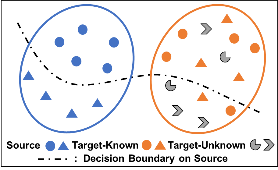
Unsupervised Domain Adaptation (UDA) means leveraging knowledge from a labeled source domain to an unlabeled target domain [5, 3, 2, 23, 12]. This adaptation implicitly assumes the source and the target data distributions, where each distribution is likely to be drawn from different distributions, i.e., domain shift (see Figure 1(a)). Researchers have approached the modeling of two distributions by statistical matching [33, 46, 24, 25], or domain adversarial learning [11, 47, 27]. Among them, domain adversarial learning has been successful in matching between the source and the target distributions via feature alignment, so the model can accomplish the domain-invariant representations.

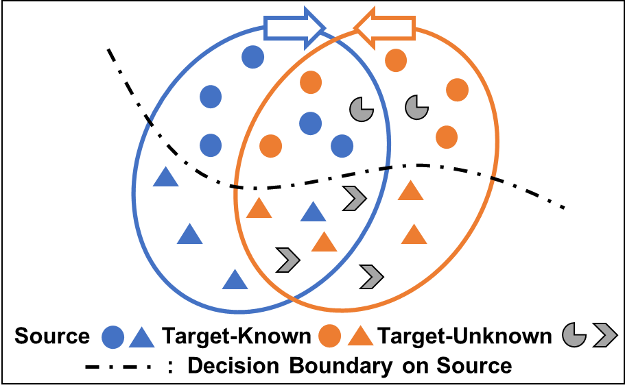
There is another dynamic aspect of the source and the target distribution. In a realistic scenario, these distributions may expand a class set, which is called unknown classes. This expansion creates a field of Open-Set Domain Adaptation (OSDA) [37, 21]. Existing adversarial learning methods of UDA have limitations to solve OSDA because matching the source and the target distribution with the unknown classes may lead to the negative transfer [10] due to the class set mismatch (see Figure 1(b)).

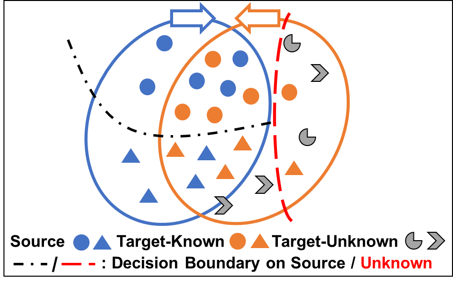
Previous OSDA methods focused on matching between the source and the target domain only embedded in the known class set via domain adversarial learning [37, 21]. However, this known-only feature alignment may fail to learn the target-unknown feature space because of no alignment signal from the target-unknown instances. Therefore, a classifier is not able to learn a clear decision boundary for unknown classes because the target-unknown instances are not segregated enough in the aligned feature space (see Figure 1(c)). On the other hand, some OSDA methods propose to learn intrinsic target structures by utilizing self-supervised learning without distribution matching [38, 20]. However, this weakens the model performance under large domain shifts. Therefore, in order to robustly solve OSDA, distribution matching via the domain adversarial learning is required, and the class set mismatch should be resolved to prevent the negative transfer, simultaneously.

(a) Domain Shift

(b) DANN [12]

(c) STA [21]

(d) UADAL (ours)

Figure 1: The feature distributions from the source and the target domain, with the decision boundaries. The blue/orange/gray arrows represent the alignment signal on the source/target-known/target-unknown domain.

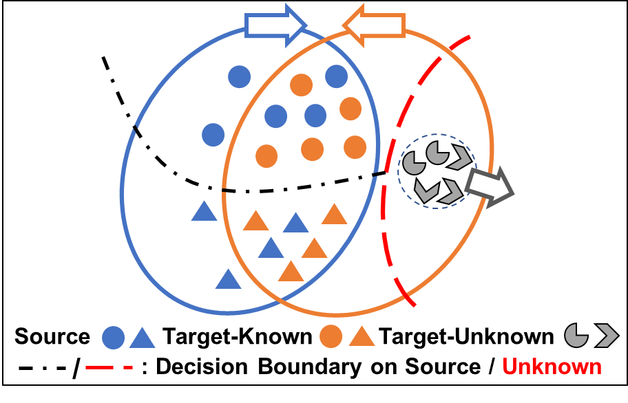
This paper proposes a new domain adversarial learning for OSDA, called Unknown-Aware Domain Adversarial Learning (UADAL). Specifically, we aim at enforcing the target-unknown features to move apart from the source and the target-known features, while aligning the source and the target-known features. We call these alignments as the segregation of the target-unknown features (gray-colored arrow in Figure 1(d)). Although this distribution segregation is an essential part of OSDA, the segregation has been only implicitly modeled because of its identification on the target-unknown instances. UADAL is the first explicit mechanism to simultaneously align and segregate the three sets (source, target-known, and target-unknown instances) via the domain adversarial learning. Therefore, the proposed unknown-aware feature alignment enables a classifier to learn a clear decision boundary on both known and unknown class in the feature space.

UADAL consists of three novel mechanisms. First, we propose a new domain discrimination loss to engage the target-unknown information. Second, we formulate a sequential optimization to enable the unknown-aware feature alignment, which is suitable for OSDA. We demonstrate that the optimized state of the proposed alignment is theoretically guaranteed. Third, we also suggest a posterior inference to effectively recognize target-known/unknown information without any thresholding.

2 Preliminary

2.1 Open-Set Domain Adaptation

This section provides a formal definition of OSDA. The fundamental properties are two folds: 1) the different data distributions of a source domain, $p_{s}(x,y)$, and a target domain, $p_{t}(x,y)$; and 2) the additional classes of the target domain, which were not observed in the source domain. Specifically, we define the source and the target datasets as $\chi_{s}=\{(x_{s}^{i},y_{s}^{i})\}_{i=1}^{n_{s}}$ and $\chi_{t}=\{(x_{t}^{i},y_{t}^{i})\}_{i=1}^{n_{t}}$, respectively. $y_{t}^{i}$ is not available at training under the UDA setting. Additionally, we designate $\mathcal{C}_{s}$ to be the source class set (a.k.a. a shared-known class), and $\mathcal{C}_{t}$ to be the target class set, i.e., $y_{t}^{i}\in\mathcal{C}_{t}$. OSDA dictates $\mathcal{C}_{s}\subset\mathcal{C}_{t}$ [37]. $\mathcal{C}_{t}\setminus\mathcal{C}_{s}$ is called unknown classes. In spite that there can be multiple unknown classes, we consolidate $\mathcal{C}_{t}\setminus\mathcal{C}_{s}$ as $y_{unk}$ to be a single unknown class, due to no knowledge on $\mathcal{C}_{t}\setminus\mathcal{C}_{s}$.

The learning objectives for OSDA become both 1) the optimal class classification in $\chi_{t}$ if a target instance belongs to $\mathcal{C}_{s}$, and 2) the optimal unknown classification if a target instance belongs to $\mathcal{C}_{t}\setminus\mathcal{C}_{s}$. This objective is formulated as follows, with a classifier $f$ and the cross-entropy loss function $\mathcal{L}_{ce}$,

$$\min_{f}\mathbb{E}_{p_{t}(x,y)} [\textbf{1}_{y_{t}\in\mathcal{C}_{s}}\mathcal{L}_{ce}(f(x_{t}),y_{t})+\textbf{1}_{y_{t}\in\{\mathcal{C}_{t}\setminus\mathcal{C}_{s}\}}\mathcal{L}_{ce}(f(x_{t}),y_{unk})].$$ (1)

2.2 Adversarial Domain Adaptation

We first step back from OSDA to Closed-set DA (CDA) with $\mathcal{C}_{t}\setminus\mathcal{C}_{s}=\phi$, where the domain adversarial learning is widely used. Domain-Adversarial Neural Network (DANN) [11] proposes,

$$\min_{f,G}\max_{D}\{\mathbb{E}_{p_{s}(x,y)}[\mathcal{L}_{ce}(f(G(x_{s})),y_{s})]-\mathcal{L}_{d}\}.$$ (2)

This objective assumes $G(x)$ to be a feature extractor that learns the domain-invariant features, enabled by the minimax game with a domain discriminator $D$, with respect to $\mathcal{L}_{d}$, as below.

$$\mathcal{L}_{d}=\mathbb{E}_{p_{s}(x)}\left[-\log D_{s}(G(x))\right]+\mathbb{E}_{p_{t}(x)}[-\log D_{t}(G(x))]$$ (3)

The adversarial framework adapts $G(x)$ toward the indistinguishable feature distributions between the source and the target domain by the minimax game on $D(G(x))=[D_{s}(G(x)),D_{t}(G(x))]$. Here, $D$ is set up to have a two-dimensional output to indicate either source or target domain, denoted as $D_{s}$ and $D_{t}$, respectively. Given these binarized outputs of $D$, this formulation is not appropriate to differentiate the target-known and the target-unknown features in OSDA. DANN enforces to include the target-unknown features in the distribution matching, which leads to performance degradation by negative transfer [10]. Figure 1(b) represents this undesired alignment of unknown classes.

Separate To Adapt (STA) [21] proposes a weighted domain adversarial learning, to resolve the negative transfer by utilizing a weighting scheme. Therefore, STA modifies $\mathcal{L}_{d}$ as follows,

$$\mathcal{L}_{d}^{\text{STA}}=\mathbb{E}_{p_{s}(x)}\left[-\log D_{s}(G(x))\right]+\mathbb{E}_{p_{t}(x)}[-w_{x}\log D_{t}(G(x))],$$ (4)

where $w_{x}$ represents a probability of an instance $x$ belonging to the shared-known classes. $\mathcal{L}_{d}^{\text{STA}}$ enables the domain adversarial learning to align the features from the source and the most likely target-known instances with the high weights. However, the feature extractor, $G$, is not able to move apart the target-unknown instances due to lower weights, i.e., no alignment signals (see Figure 1(c)). STA modeled this known-only feature alignment by assuming the unknown feature would be implicitly learned through the estimation on $w_{x}$. Besides learning $w_{x}$, the target-unknown instances cannot contribute to the training of STA because their loss contribution will be limited by lower $w_{x}$, in the second term of Eq. (4). Therefore, STA does not take information from the target-unknowns, and later Section 4.3 empirically shows that the target-unknown segregation of STA is limited.

2.3 Comparison to Recent OSDA Research

In terms of the domain adversarial learning, in addition to STA, OSBP [37] utilizes a classifier to predict the target instances to the pre-determined threshold, and trains the feature extractor to deceive the classifier for aligning to known classes or rejecting as unknown class. However, their recognition on unknown class only depends on the threshold value, without considering the data instances. PGL [29] introduces progressive graph-based learning to regularize the class-specific manifold, while jointly optimizing the feature alignment via domain adversarial learning. However, their adversarial loss includes all instances of the target domain, which is critically weakened by the negative transfer.

On the other hand, self-supervised learning approaches have been proposed recently, in order to exploit the intrinsic structure of the target domain [6, 38, 20]. However, these approaches do not have any feature alignments between the source and the target domain, which leads to performance degradation under significant domain shifts. There is also a notable work, OSLPP [51] optimizing projection matrix toward a common subspace to class-wisely align the source and the target domain. However, the optimization requires pair-wise distance calculation, which results in a growing complexity of $O(n^{2})$ by the $n$ data instances. It could be limited to the large-scale domain. We provide detailed comparisons and comprehensive literature reviews in Appendix A.

(a) The overall structure of UADAL

(b) The optimization procedure of UADAL

Figure 2: Overview of the proposed Unknown-Aware Domain Adversarial Learning (UADAL) approach.

3 Methodology

3.1 Overview of UADAL

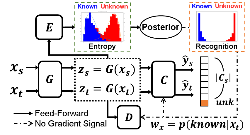
Figure 2(a) illustrates the neural network compositions and the information flow. Our model consists of four networks: 1) a feature extractor, $G$; 2) a domain discriminator, $D$; 3) an open-set recognizer, $E$; and 4) a class classifier network, $C$. The networks $G$, $D$, $E$, and $C$ are parameterized by $\theta_{g},\theta_{d},\theta_{e}$, and $\theta_{c}$, respectively. First, we propose a new domain discrimination loss, and we formulate the sequential optimization problem, followed by theoretical analyses. In order to recognize target-unknown information, we introduce a posterior inference method, followed by open-set classification.

3.2 Sequential Optimization Problem for Unknown-Aware Feature Alignment

Model Structure We assume that we identify three domain types, which are 1) the source (s), 2) the target-known (tk), and 3) and target-unknown (tu). As the previous works such as STA and DANN utilize a two-way domain discriminator with ($D_{s}$, $D_{t}$), they can treat only s and tk (or t). However, a domain discriminator in OSDA should be able to handle tu information for segregation. Therefore, we designed the discriminator dimension to be three ($D_{s}$, $D_{tk}$, $D_{tu}$), as follows,

$$D(G(x))=[D_{s}(G(x)),D_{tk}(G(x)),D_{tu}(G(x))].$$ (5)

Given these three dimensions of $D$, we propose new domain discrimination losses, $\mathcal{L}_{d}^{s}$ and $\mathcal{L}_{d}^{t}$, as

$$\begin{split}\mathcal{L}_{d}^{s}(\theta_{g},\theta_{d})={}&\mathbb{E}_{p_{s}(x)}\left[-\log D_{s}(G(x))\right],\end{split}$$ (6)

$$\begin{split}\mathcal{L}_{d}^{t}(\theta_{g},\theta_{d})={}&\mathbb{E}_{p_{t}(x)}[\ -w_{x}\log D_{tk}(G(x))-(1-w_{x})\log D_{tu}(G(x))],\end{split}$$ (7)

where $w_{x}:=p(\textit{known}|x)$, named as open-set recognition, is the probability of a target instance, $x$, belonging to a shared-known class. We introduce the estimation of this probability, $w_{x}$, in the section 3.4 later. From $\mathcal{L}_{d}^{t}$ in Eq. (7), our modified $D$ becomes to be able to discriminate tk and tu, explicitly.

Our new unknown awareness of $D$ allows us to segregate the target-unknown features via the domain adversarial learning framework. Firstly, we decompose $\mathcal{L}_{d}^{t}(\theta_{g},\theta_{d})$ into $\mathcal{L}_{d}^{tk}(\theta_{g},\theta_{d})$ and $\mathcal{L}_{d}^{tu}(\theta_{g},\theta_{d})$,

$$\mathcal{L}_{d}^{t}(\theta_{g},\theta_{d})=\mathcal{L}_{d}^{tk}(\theta_{g},\theta_{d})+\mathcal{L}_{d}^{tu}(\theta_{g},\theta_{d}),$$ (8)

$$\begin{split}\mathcal{L}_{d}^{tk}(\theta_{g},\theta_{d}):={}&\lambda_{tk}\mathbb{E}_{p_{tk}(x)}\left[-\log D_{tk}(G(x))\right],\end{split}$$ (9)

$$\begin{split}\mathcal{L}_{d}^{tu}(\theta_{g},\theta_{d}):={}&\lambda_{tu}\mathbb{E}_{p_{tu}(x)}\left[-\log D_{tu}(G(x))\right],\end{split}$$ (10)

where $p_{tk}(x):=p_{t}(x|\textit{known})$, $p_{tu}(x):=p_{t}(x|\textit{unknown})$, $\lambda_{tk}:=p(\textit{known})$, and $\lambda_{tu}:=p(\textit{unknown})$. The derivation of Eq. (8) is based on $p_{t}(x)=\lambda_{tk}p_{tk}(x)+\lambda_{tu}p_{tu}(x)$, which comes from the law of total probability (Details in Appendix B.1.1). Therefore, this decomposition of $\mathcal{L}_{d}^{t}$ into $\mathcal{L}_{d}^{tu}$ and $\mathcal{L}_{d}^{tk}$ enables the different treatments on tk and tu feasible. The three-way discriminator and its utilization in Eq. (9)-(10) becomes the unique contribution from UADAL.

Optimization Our goal of this unknown-aware domain discrimination is to align the features from the source and the target-known instances while simultaneously segregating the target-unknown features. To achieve this goal, we propose a new sequential optimization problem w.r.t. $G$ and $D$. Based on the losses, $\mathcal{L}_{d}^{s}(\theta_{g},\theta_{d})$, $\mathcal{L}_{d}^{tk}(\theta_{g},\theta_{d})$, and $\mathcal{L}_{d}^{tu}(\theta_{g},\theta_{d})$, we formulate the optimization problem as,

$$\begin{split}\min_{\theta_{d}}\ \mathcal{L}_{D}(\theta_{g},\theta_{d})&=\mathcal{L}_{d}^{s}(\theta_{g},\theta_{d})+\ \mathcal{L}_{d}^{tk}(\theta_{g},\theta_{d})+\mathcal{L}_{d}^{tu}(\theta_{g},\theta_{d}),\end{split}$$ (11)

$$\begin{split}\max_{\theta_{g}}\ \mathcal{L}_{G}(\theta_{g},\theta_{d})&=\mathcal{L}_{d}^{s}(\theta_{g},\theta_{d})+\ \mathcal{L}_{d}^{tk}(\theta_{g},\theta_{d})-\mathcal{L}_{d}^{tu}(\theta_{g},\theta_{d}).\end{split}$$ (12)

This alternating objective by Eq. (11) and Eq. (12) is equivalent to the adversarial domain adaptation models [11, 21] to learn the domain-invariant features. Unlike the previous works, however, Eq. (11) represents that we train the domain discriminator, $D$, to classify an instance as either source, target-known, or target-unknown domain. In terms of the feature extractor, $G$, we propose Eq. (12) to maximize the domain discrimination loss for the source and the target-known domain while minimizing the loss for the target-unknown domain. From the different signals on $\mathcal{L}_{d}^{tk}$ and $\mathcal{L}_{d}^{tu}$, we only treat the adversarial effects on $\mathcal{L}_{d}^{s}$ and $\mathcal{L}_{d}^{tk}$. Meanwhile, minimizing $\mathcal{L}_{d}^{tu}$ provides for the network $G$ to learn the discriminative features on $tu$. Eventually, $G$ and $D$ align the source and target-known features and segregate the target-unknown features from the source and the target-known features (the optimization details in Figure 2(b)). We provide the theoretic analysis of the optimized state of the proposed feature alignment in the next subsection, which is unexplored in the OSDA field.

3.3 Theoretic Analysis of Sequential Optimization

This section provides a theoretic discussion on the proposed feature alignment by our sequential optimization, w.r.t. Eq. (11)-(12). Since our ultimate goal is training $G$ to learn unknown-aware feature alignments, we treat $G$ as a leader and $D$ as a follower in the game theory. We first optimize Eq. (11) to find $D^{*}$ with a fixed $G$. The optimal $D^{*}$ given the fixed $G$ results in the below output :

$$D^{*}(z)=\Big{[}\frac{p_{s}(z)}{2p_{avg}(z)},\frac{\lambda_{tk}p_{tk}(z)}{2p_{avg}(z)},\frac{\lambda_{tu}p_{tu}(z)}{2p_{avg}(z)}\Big{]},$$ (13)

where $p_{avg}(z)=(p_{s}(z)+\lambda_{tk}p_{tk}(z)+\lambda_{tu}p_{tu}(z))/2$ (Details in Appendix B.1.2). Here, $z\in\mathcal{Z}$ stands for the feature space from $G$, i.e., $p_{d}(z)=\{G(x;\theta_{g})|x\sim p_{d}(x)\}$ where $d$ is $s$, $tk$, or $tu$. Given $D^{*}$ with the optimal parameter $\theta^{*}_{d}$, we optimize $G$ in Eq. (12). Here, we show that the optimization w.r.t. $G$ is equivalent to the weighted summation of KL Divergences, by Theorem 14.

Theorem 3.1.

(Proof in Appendix B.1.3) Let $\theta^{*}_{d}$ be the optimal parameter of $D$ by optimizing Eq. (11). Then, $-\mathcal{L}_{G}(\theta_{g},\theta^{*}_{d})$ can be expressed as, with a constant $C_{0}$,

$$\begin{split}-\mathcal{L}_{G}(\theta_{g},\theta^{*}_{d})=D_{KL}(p_{s}\|p_{avg})+\lambda_{tk}D_{KL}(p_{tk}\|p_{avg})-\lambda_{tu}D_{KL}(p_{tu}\|p_{avg})+C_{0}.\end{split}$$ (14)

We note that $p_{s},p_{tk}$, and $p_{tu}$ are the feature distribution of each domain, mapped by $G$, respectively. Therefore, we need to minimize Eq. (14) to find the optimal $G^{*}$. Having observed Theorem 14, Eq. (14) requires $p_{tu}$ to have a higher deviation from the average distribution, $p_{avg}$, while matching towards $p_{s}\approx p_{avg}$ and $p_{tk}\approx p_{avg}$. From this optimization procedure, we obtain the domain-invariant features over the source and the target-known domain, while segregating the target-unknowns, which is formalized as $p_{s}\approx p_{tk}$ and $p_{tu}\leftrightarrow\{p_{tk},p_{s}\}$. We show that minimizing Eq. (14) does not lead to the negative infinity by the third term, regardless of the other KL Divergences, by Proposition 3.2.

Proposition 3.2.

(Proof in Appendix B.1.4) $D_{KL}(p_{tu}\|p_{avg})$ is bounded to $\log 2-\log{\lambda_{tu}}$.

This boundness guarantees that the first two KL Divergence terms maintain their influence on optimizing the parameter $\theta_{g}$ of $G$ stably while segregating the target-unknown features. Furthermore, we show Proposition 3.3 to characterize the feature alignment between $p_{s}$ and $p_{tk}$ under Eq. (14).

Proposition 3.3.

(Proof in Appendix B.1.5) Assume that $\text{supp}(p_{s})\cap\text{supp}(p_{tu})=\emptyset$ and $\text{supp}(p_{tk})\cap\text{supp}(p_{tu})=\emptyset$, where $\text{supp}(p):=\{z\in\mathcal{Z}|p(z)>0\}$ is the support set of $p$. Then, the minimization w.r.t. $G$, by Eq. (14), is equivalent to the minimization of the summation on two $f$-divergences:

$$D_{f_{1}}(p_{s}||p_{tk})+\lambda_{tk}D_{f_{2}}(p_{tk}||p_{s}),$$

where $f_{1}(u)=u\log\frac{u}{(1-\alpha)u+\alpha}$ and $f_{2}(u)=u\log\frac{u}{\alpha u+(1-\alpha)}$, with $\alpha=\frac{\lambda_{tk}}{1+\lambda_{tk}}$. Therefore, the minimum of Eq. (14) is achieved if and only if $p_{s}=p_{tk}$.

Therefore, under the assumption, Proposition 3.3 theoretically guarantees that the source and the target-known feature distributions are aligned, which represents $p_{s}=p_{tk}$. From these analyses, we can theoretically guarantee both alignment and segregation from the proposed optimization.

3.4 Open-Set Recognition via Posterior Inference

This section starts from estimating $w_{x}=p(\textit{known}|x)$ for a target instance, $x$. First, we utilize the labeled source dataset, $\chi_{s}$, to train the feature extractor $G$ and the open-set recognizer $E$, as below,

$$\mathcal{L}_{e}^{s}(\theta_{g},\theta_{e})=\frac{1}{n_{s}}\sum_{(x_{s},y_{s})\in\chi_{s}}\mathcal{L}_{ce}(E(G(x_{s})),y_{s}),$$ (15)

where $E(G(x))\in\mathbb{R}^{|\mathcal{C}_{s}|}$ contains the softmax activation. We note that the open-set recognizer, $E$, is a classifier to learn the decision boundary over $\mathcal{C}_{s}$ by the source domain.

Given the decision boundary by $E$, our assumption for open-set recognition includes two statements: for the target instances, 1) the higher entropy is caused by an uncertain classification case, and 2) the unknown class may induce the higher entropy because there are no prior training instances in the unknown classes. Based on two assumptions, the open-set recognizer, $E$, will provide higher entropy for the target-unknown instances than the target-known instances. Therefore, we consider the entropy value as the open-set recognition indicator. We verified our assumptions empirically in Figure 9.

While we notice the entropy value from a single instance as the indicator between known and unknown, the open-set recognition should be holistically modeled over the target domain. Therefore, we model the mixture of two Beta distributions on the normalized target entropy values as below,

$$p(\ell_{x})=\lambda_{tk}p(\ell_{x}|\textit{known})+\lambda_{tu}p(\ell_{x}|\textit{unknown}),$$ (16)

where the definition of $\lambda_{tk}$ and $\lambda_{tu}$ is the same as in the previous subsection. $\ell_{x}$ is the entropy value for the target instance, $x$, i.e., $\ell_{x}=H(E(G(x)))$ with the entropy function $H$. The Beta distribution is a perfect fit for this case of the closed interval support of $[0,1]$, which is the normalized range of the entropy. Thus, we introduce the estimator $\hat{w}_{x}$ of $w_{x}$ by Posterior Inference, from fitting the Beta mixture model through the Expectation-Maximization (EM) algorithm (Details in Appendix B.2.1),

$$\hat{w}_{x}:=p(\textit{known}|\ell_{x})=\frac{\lambda_{tk}p(\ell_{x}|known)}{\lambda_{tk}p(\ell_{x}|\textit{known})+\lambda_{tu}p(\ell_{x}|\textit{unknown})},$$ (17)

where the denominator is from Eq. (16). Since the fitting process incorporates all target information, the entire dataset is utilized to set a more informative weighting without any thresholds. Here, $\lambda_{tk}$ and $\lambda_{tu}$ are also explicitly estimated by the EM algorithm since they are not given (see Eq. (41) in Appendix B.2.1), whereas a threshold hyperparameter is used by the previous researches [29, 51].

3.5 Open-Set Classification

Given the proposed feature alignments, we train a classifier, $C$, to correctly classify the target instance over $\mathcal{C}_{s}$ or to reject as unknown. Note that the classifier, $C$, is the extended classifier with the dimension of $|\mathcal{C}_{s}|+1$ to include the unknown class. Firstly, we construct the source classification loss on $\chi_{s}$. Secondly, for the target domain, we need to learn the decision boundary for the unknown class. Based on the proposed open-set recognition, $\hat{w}_{x}$, we train the classifier, $C$, as follows:

$$\mathcal{L}_{cls}(\theta_{g},\theta_{c})=\frac{1}{n_{s}}\sum_{(x_{s},y_{s})\in\chi_{s}}\mathcal{L}_{ce}(C(G(x_{s})),y_{s})+\frac{1}{{n_{t}}^{\prime}}\sum_{x_{t}\in\chi_{t}}(1-\hat{w}_{x})\mathcal{L}_{ce}(C(G(x_{t})),y_{unk}),$$ (18)

where ${n_{t}}^{\prime}$ is a normalizing constant, and $y_{unk}$ is the one-hot vector for the unknown class. Furthermore, we incorporate entropy minimization loss for enforcing the unlabeled target instances to be recognized effectively [15, 21, 6], with the entropy loss function, $\mathcal{L}_{H}$,

$$\mathcal{L}_{ent}^{t}(\theta_{g},\theta_{c})= \frac{1}{n_{t}}\sum_{x_{t}\in\chi_{t}}\mathcal{L}_{H}(C(G(x_{t}))).$$ (19)

3.6 Conditional UADAL

Domain adversarial learning may fail to capture a class-wise discriminative pattern in the features when the data distributions are complex [26]. Therefore, we also experimented with the conditional UADAL (cUADAL) with the discriminative information between classes. Inspired by [26], we replace the input information of the domain discriminator, $D$, from $G(x)$ to $[G(x),C(x)]$ in Eq. (6)-(7). cUADAL has the conditions on the prediction of the extended classifier, $C$, which is including the unknown dimension. Therefore, cUADAL provides more discriminative information than UADAL.

3.7 Training Procedure

We introduce how to update the networks, $E$, $G$, $D$, and $C$, based on the proposed losses. Before we start the training, we briefly fit the parameters of the posterior inference to obtain $\hat{w}_{x}$. This starting stage trains $E$ and $G$ on the source domain with a few iterations to catch the two modalities of the target entropy values, inspired by the previous work [1], as below,

$$(\hat{\theta}_{e},\hat{\theta}_{g})=\operatorname{argmin}_{\theta_{g},\theta_{e}}\mathcal{L}_{e}^{s}(\theta_{g},\theta_{e}).$$ (20)

After the initial setup of $\hat{w}_{x}$, we train $D$, $C$, $E$, and $G$, alternatively. This alternation is composed of two phases: (i) learning $D$; and (ii) learning $G$, $C$, and $E$ networks. The first phase of the alternative iterations starts from learning the domain discriminator, $D$, by the optimization on $\mathcal{L}_{D}$ in Eq. (11),

$$\hat{\theta}_{d}=\operatorname{argmin}_{\theta_{d}}\mathcal{L}_{D}(\theta_{g},\theta_{d}).$$ (21)

Based on the updated $\hat{\theta}_{d}$, the parameter, $\theta_{g}$, is associated with both optimization loss and classification loss. Therefore, for the second phase, the parameters, $\theta_{g}$ and $\theta_{c}$, are optimized as below,

$$(\hat{\theta}_{g},\hat{\theta}_{c})={}\operatorname{argmin}_{\theta_{g},\theta_{c}}\mathcal{L}_{cls}(\theta_{g},\theta_{c})+\mathcal{L}_{ent}^{t}(\theta_{g},\theta_{c})-\mathcal{L}_{G}(\theta_{g},\hat{\theta}_{d}).$$ (22)

We also keep updating $\theta_{e}$ by Eq. (20), which leads to a better fitting of the posterior inference on the aligned features (empirically shown in Figure 9). Algorithm 1 in Appendix B.3.1 enumerates the detailed training procedures of UADAL. Computational Complexity is asymptotically the same as existing domain adversarial learning methods, which linearly grow by the number of instances $O(n)$. The additional complexity may come from the posterior inference requiring $O(nk)$; $k$ is a constant number of EM iterations (the detailed analysis on the computations in Appendix B.3.2 and C.2.8).

4 Experiments

4.1 Experimental Settings

Datasets We utilized several benchmark datasets. Office-31 [36] consists of three domains: Amazon (A), Webcam (W), and DSLR (D) with 31 classes. Office-Home [50] is a more challenging dataset with four different domains: Artistic (A), Clipart (C), Product (P), and Real-World (R), containing 65 classes. VisDA [34] is a large-scale dataset from synthetic images to real one, with 12 classes. In terms of the class settings, we follow the experimental protocols by [37].

Baselines We compared UADAL and cUADAL with several baselines by choosing the recent works in CDA, OSDA, and Universal DA (UniDA). For CDA, we choose DANN [11] and CDAN [26] to show that the existing domain adversarial learning for CDA is not suitable for OSDA. For OSDA, we compare UADAL to OSBP [37], STA [21], PGL [29], ROS [6], and OSLPP [51]. For UniDA, we conduct the OSDA setting in DANCE [38] and DCC [20].

Implementation We commonly utilize three alternative pre-trained backbones: 1) ResNet-50 [16], 2) DenseNet-121 [17], and 3) EfficientNet-B0 [45] to show the robustness on backbone network choices, while using VGGNet [41] on VisDA for a fair comparison. (Details in Appendix C.1).

Metric We utilize HOS, which is a harmonic mean of OS^∗, and UNK [6]. OS^∗ is a class-wise averaged accuracy over known classes, and UNK is an accuracy only for the unknown class. HOS is suitable for OSDA because it is higher when performing well in both known and unknown classifications.

Backbone (#)/		Office-31							Office-Home
Model		A-W	A-D	D-W	W-D	D-A	W-A	Avg.	P-R	P-C	P-A	A-P	A-R	A-C	R-A	R-P	R-C	C-R	C-A	C-P	Avg.
EfficientNet-B0 (5.3M)	DANN	63.2	72.7	92.6	94.8	63.7	57.2	74.0$\pm$0.3	35.7	16.5	18.2	34.1	46.3	22.9	40.7	47.8	28.2	12.4	7.5	13.4	27.0$\pm$0.3
	CDAN	65.5	73.6	92.4	94.6	64.8	57.9	74.8$\pm$0.2	37.9	18.1	20.4	35.6	47.0	24.6	44.1	49.8	30.1	13.5	8.9	15.0	28.8$\pm$0.6
	STA	58.3	62.2	81.6	79.6	69.8	67.4	69.8$\pm$1.2	59.4	43.6	51.9	53.8	60.6	49.5	58.8	53.5	49.9	53.4	49.5	49.4	52.8$\pm$0.2
	OSBP	82.9	87.0	33.8	96.7	27.3	69.9	66.3$\pm$2.1	65.0	46.0	58.6	64.2	71.0	54.0	58.3	62.5	50.3	63.7	50.7	55.6	58.3$\pm$1.6
	ROS	69.7	80.1	94.7	99.6	73.0	59.2	79.4$\pm$0.3	66.9	44.9	53.7	62.5	69.5	50.0	62.0	67.0	52.0	61.2	50.5	54.7	57.9$\pm$0.1
	DANCE	68.1	68.8	91.3	85.0	68.5	63.3	74.2$\pm$4.0	17.2	47.5	7.2	26.6	19.6	36.6	2.2	19.8	10.9	6.4	4.3	19.0	18.1$\pm$2.9
	DCC	87.2	69.1	89.4	94.4	63.5	76.1	79.9$\pm$2.9	72.2	41.0	56.5	66.4	75.7	52.8	55.9	71.5	49.9	60.4	48.1	60.8	59.3$\pm$1.5
	UADAL	87.5	88.3	97.4	96.9	74.1	68.9	85.5$\pm$0.5	75.0	50.0	62.9	66.4	74.1	52.7	71.5	72.6	53.6	65.3	60.8	63.7	64.1$\pm$0.1
	cUADAL	86.5	89.1	97.3	98.0	72.5	71.0	85.7$\pm$0.7	74.7	54.4	64.2	66.3	73.9	50.8	71.4	73.0	52.4	65.3	61.0	63.3	64.2$\pm$0.1
DenseNet-121 (7.9M)	DANN	71.9	72.0	90.2	85.3	73.8	72.3	77.6$\pm$0.5	68.8	35.4	48.7	62.6	71.9	45.3	62.8	68.7	45.9	62.2	47.0	54.7	56.2$\pm$0.3
	CDAN	69.5	69.8	86.8	84.5	73.8	72.5	76.2$\pm$0.2	68.9	39.2	51.9	62.6	71.8	47.1	63.6	68.0	48.7	62.8	49.3	55.2	57.4$\pm$0.3
	STA	77.0	68.6	84.0	77.2	76.6	75.1	76.4$\pm$1.5	65.6	46.1	58.4	55.8	64.3	50.4	62.6	58.6	51.1	61.0	56.0	55.9	57.1$\pm$0.1
	OSBP	81.9	83.0	88.9	96.6	73.1	74.9	83.1$\pm$2.2	71.9	46.0	60.3	67.1	72.3	54.5	65.9	71.7	53.7	66.8	59.3	64.1	62.8$\pm$0.1
	ROS	67.0	67.8	97.4	99.4	77.1	71.8	80.1$\pm$1.3	73.0	49.6	59.2	67.8	75.5	52.8	66.4	74.6	54.3	64.8	53.0	57.8	62.4$\pm$0.1
	DANCE	69.9	67.8	84.0	82.8	79.9	81.1	77.6$\pm$0.3	51.8	51.0	59.7	63.9	58.2	58.2	43.4	48.9	55.0	41.3	54.6	60.6	53.9$\pm$0.5
	DCC	83.9	80.8	88.4	93.1	79.7	80.4	84.4$\pm$1.3	75.1	46.6	58.0	70.8	78.6	56.6	63.4	75.5	55.8	71.3	55.0	63.3	64.2$\pm$0.2
	UADAL	86.0	82.3	96.7	99.2	77.9	74.2	86.0$\pm$0.6	75.7	45.5	61.5	70.0	76.9	57.3	71.5	76.1	60.4	70.0	60.1	67.2	66.0 $\pm$0.2
	cUADAL	85.1	83.6	96.4	99.6	77.5	75.9	86.4$\pm$0.6	75.6	48.9	61.7	70.0	76.7	57.8	71.9	76.7	59.1	69.6	60.1	67.5	66.3$\pm$0.3
ResNet-50 (25.5M)	DANN	68.1	71.5	86.7	82.5	73.7	72.6	75.9$\pm$0.5	69.8	44.6	56.3	65.2	71.0	51.2	65.4	68.4	50.9	66.7	57.6	60.9	60.7$\pm$0.2
	CDAN	64.9	66.8	84.3	80.5	72.7	71.0	73.4$\pm$1.3	69.7	47.2	58.6	65.1	70.7	52.9	66.0	67.6	52.7	67.1	58.2	61.7	61.4$\pm$0.3
	STA∗	75.9	75.0	69.8	75.2	73.2	66.1	72.5$\pm$0.8	69.5	53.2	61.9	54.0	68.3	55.8	67.1	64.5	54.5	66.8	57.4	60.4	61.1$\pm$0.3
	OSBP∗	82.7	82.4	97.2	91.1	75.1	73.7	83.7$\pm$0.4	73.9	53.2	63.2	65.2	72.9	55.1	66.7	72.3	54.5	70.6	64.3	64.7	64.7$\pm$0.2
	PGL∗	74.6	72.8	76.5	72.2	69.5	70.1	72.6$\pm$1.5	41.6	46.6	47.2	45.6	55.8	29.3	11.4	52.5	0.0	45.6	10.0	36.8	35.2
	ROS∗	82.1	82.4	96.0	99.7	77.9	77.2	85.9$\pm$0.2	74.4	56.3	60.6	69.3	76.5	60.1	68.8	75.7	60.4	68.6	58.9	65.2	66.2$\pm$0.3
	DANCE	66.9	70.7	80.0	84.8	65.8	70.2	73.1$\pm$1.0	41.2	55.7	54.2	49.8	39.4	53.1	27.5	44.0	48.3	30.2	40.9	45.9	44.2$\pm$0.6
	DCC∗	87.1	85.5	91.2	87.1	85.5	84.4	86.8	64.0	52.8	59.5	67.4	80.6	52.9	56.0	62.7	76.9	67.0	49.8	66.6	64.2
	OSLPP∗	89.0	91.5	92.3	93.6	79.3	78.7	87.4	74.0	59.3	63.6	72.8	74.3	61.0	67.2	74.4	59.0	70.4	60.9	66.9	67.0
	UADAL	89.1	86.0	97.8	99.5	79.7	76.5	88.1$\pm$0.2	76.9	56.6	63.0	70.8	77.4	63.2	72.1	76.8	60.6	73.4	64.2	69.5	68.7$\pm$0.2
	cUADAL	90.1	87.9	98.2	99.4	80.5	75.1	88.5$\pm$0.3	76.8	54.6	62.9	71.6	77.5	63.6	72.6	76.7	59.9	72.6	65.0	68.3	68.5$\pm$0.1

Table 1: HOS score (%) on Office-31 & Office-Home using EfficientNet-B0 (5.3M), DenseNet-121 (7.9M), and ResNet-50 (25.5M) as backbone network, where (#) represents the number of the parameters. A-W in a column means that A is the source domain and W is the target domain. Avg. is the averaged HOS over all tasks in each dataset. (bold: best performer, underline: second-best performer, ^∗: officially reported performances.) The detailed experimental results including the other metrics such as OS^∗ and UNK are in Appendix C.2.9

Method	EfficientNet-B0			DenseNet-121			ResNet-50			VGGNet
	OS*	UNK	HOS	OS*	UNK	HOS	OS*	UNK	HOS	OS*	UNK	HOS
STA	49.3	56.4	52.5	53.1	76.7	62.7	56.9	75.8	65.0	63.9∗	84.2∗	72.7∗
OSBP	48.8	70.4	57.6	48.7	65.7	55.9	50.0	77.2	60.7	59.2∗	85.1∗	69.8∗
PGL	56.9	26.1	35.8	-	-	-	70.3	33.4	45.3	82.8∗	68.1∗	74.7∗
ROS	36.7	72.0	48.7	42.7	81.1	55.9	45.8	64.8	53.7	-	-	-
DANCE	38.9	63.2	48.1	59.8	67.3	62.3	61.3	72.9	66.5	-	-	-
DCC	38.3	54.2	44.8	16.7	76.9	27.2	13.4	88.0	23.3	68.0∗	73.6∗	70.7∗
OSLPP	-	-	-	-	-	-	-	-	-	-	-	-
UADAL	47.0	76.8	58.3	56.2	81.5	66.5	58.0	86.2	69.4	63.1	93.3	75.3
cUADAL	47.2	76.5	58.4	57.9	84.1	68.6	58.5	87.6	70.1	64.3	92.6	75.9

Table 2: Results on VisDA dataset. (bold/underline/^∗: Refer to the Table 1)

Office-31 with ResNet-50
Weight	Core	HOS Avg.
STA	STA	72.5$\pm$0.8
	UADAL	85.5$\pm$0.9
ROS	ROS	85.9$\pm$0.2
	UADAL	86.7$\pm$0.2
UADAL	UADAL	88.1$\pm$0.2

Table 3: Ablation Studies for Different Weighting / Core Schemes on STA and ROS.

4.2 Experimental Results

Quantitative Analysis Table 1 reports the quantitative performances of UADAL, cUADAL, and baselines applied to Office-31 and Office-Home, with three backbone networks. UADAL and cUADAL show statistically significant improvements compared to all existing baselines in both Office-31 and Office-Home. Moreover, there is a large improvement by UADAL from baselines in EfficientNet-B0 and DenseNet-121, even with fewer parameters. In terms of the table on ResNet-50, for a fair comparison, UADAL outperforms the most competitive model, OSLPP (HOS=67.0). Compared to the domain adversarial learning methods, such as STA and OSBP, UADAL significantly outperforms in all cases. UADAL also performs better than other self-supervised learning methods such as ROS and DCC. These performance increments are commonly observed in all three backbone structures and in two benchmark datasets, which represents the effectiveness of the proposed model.

Table 2 shows the experimental results on VisDA, which is known to have a large domain shift from a synthetic to a real domain. It demonstrates that UADAL and cUADAL outperform the other baselines under the significant domain shift. Moreover, the baselines with the feature alignments by the domain adversarial learning, such as STA, OSBP, and PGL, outperform the self-supervised learning models, ROS, DANCE, and DCC, in most cases. Therefore, these results support that OSDA essentially needs the feature alignments when there are significant domain shifts. The detailed discussions about the low accuracies of some baselines are in Appendix C.2.2. In addition, we observe that cUADAL mostly performs better than UADAL, which shows that cUADAL provides more discriminative information both on known and unknown by the prediction of the classifier $C$.

(a) DANN

(b) STA

(c) cUADAL

Figure 3: t-SNE Visualization on D $\rightarrow$ W of Office-31. (Blue/Red/Green: Target-Known/-Unknown/Source)

Figure 4: PAD value on tk/tu feature distributions.

Figure 5: Openness on Office-31 (ResNet-50).

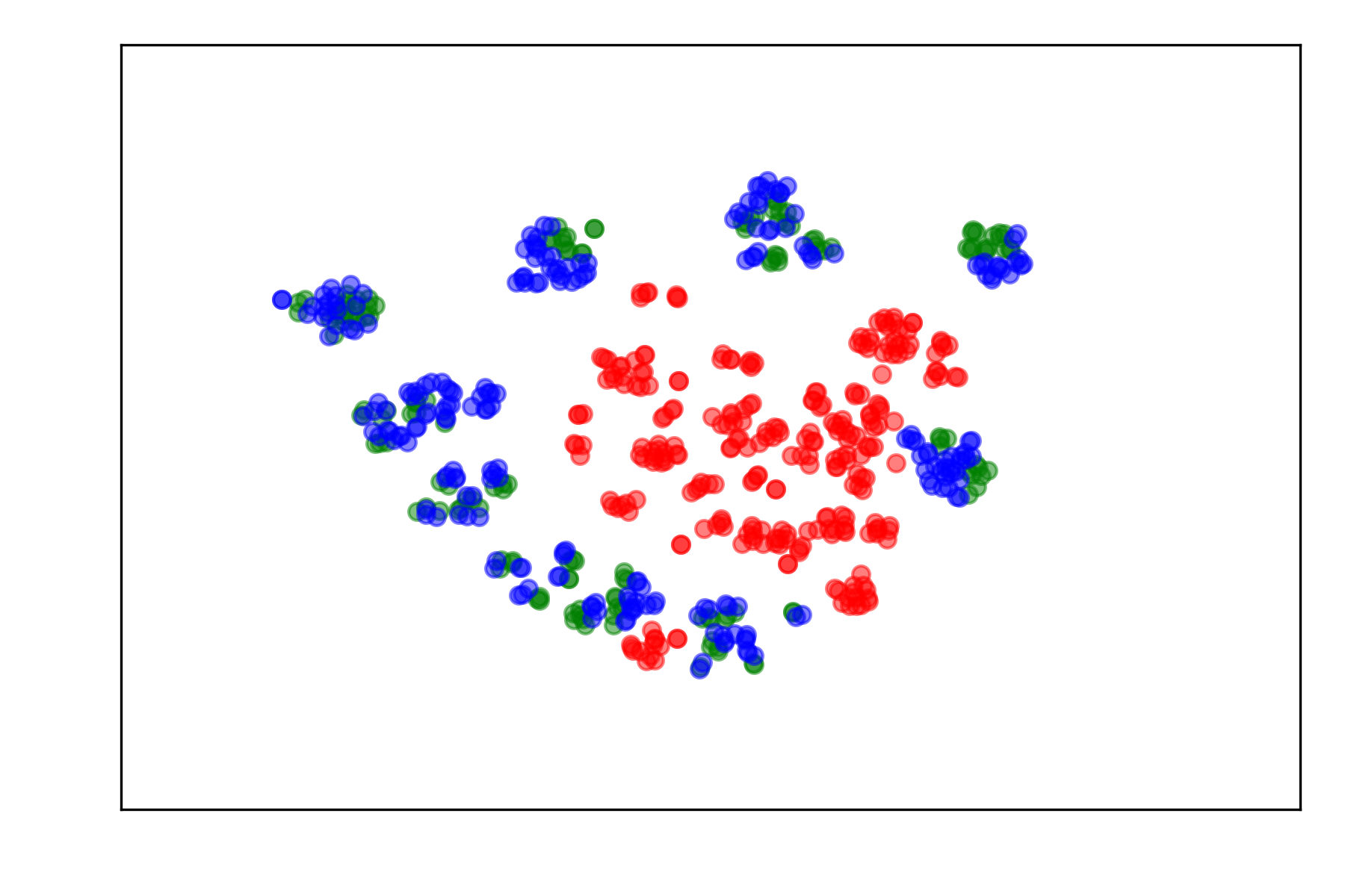
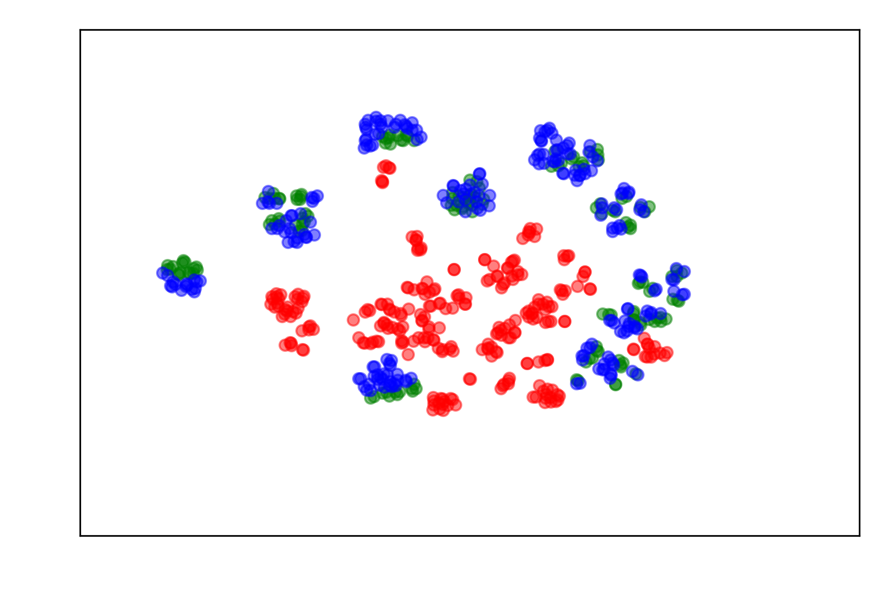
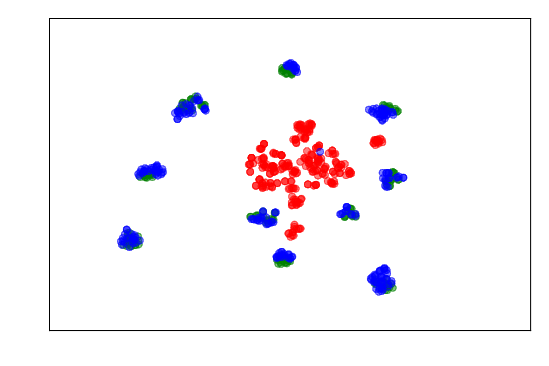
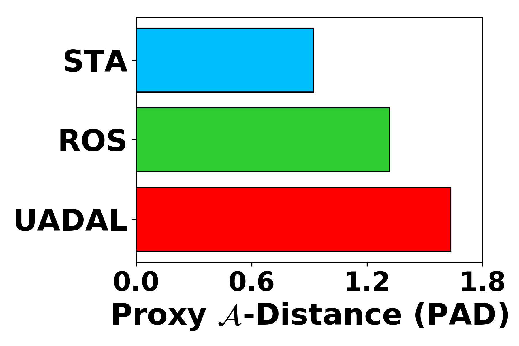
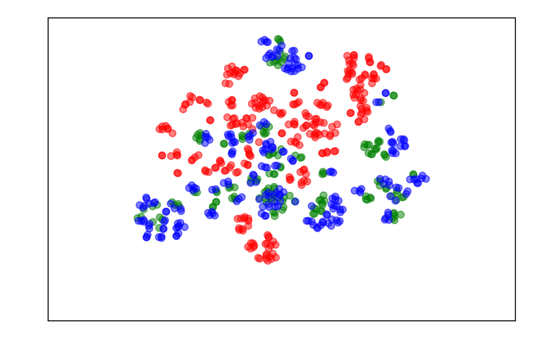
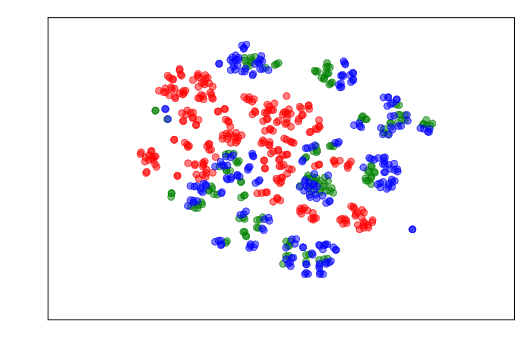
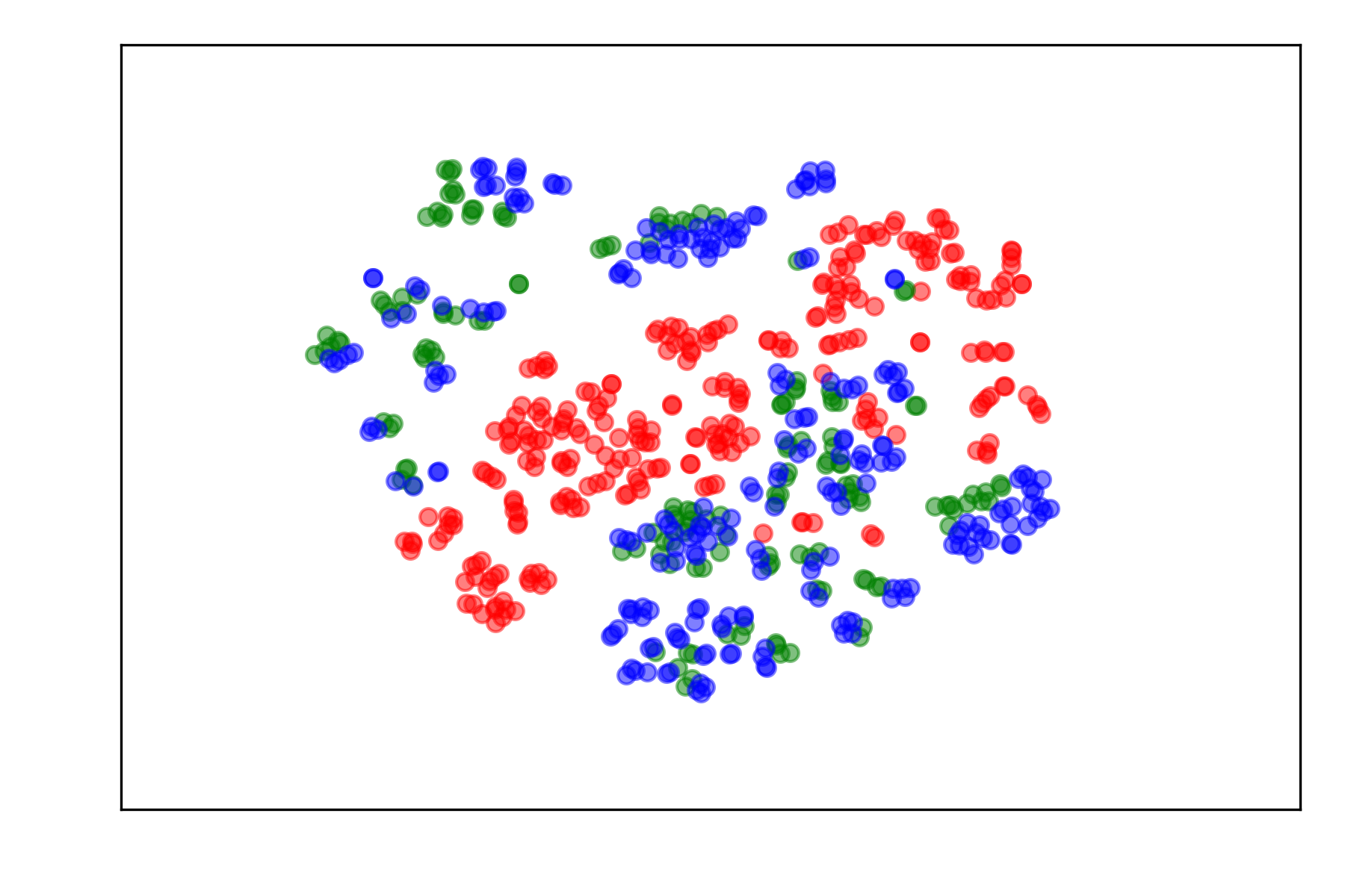
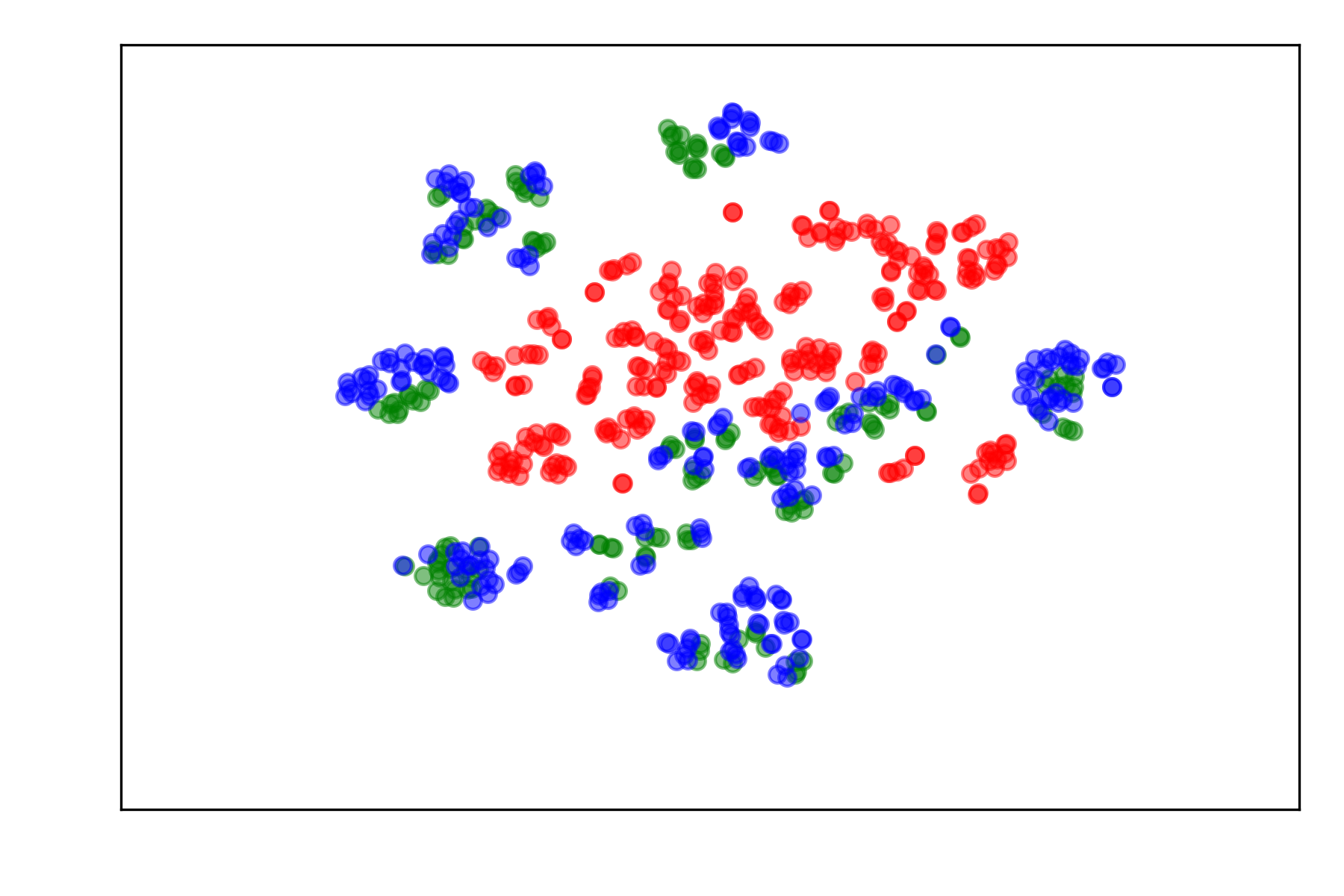
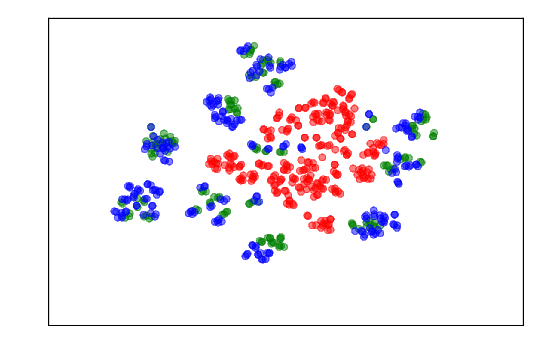
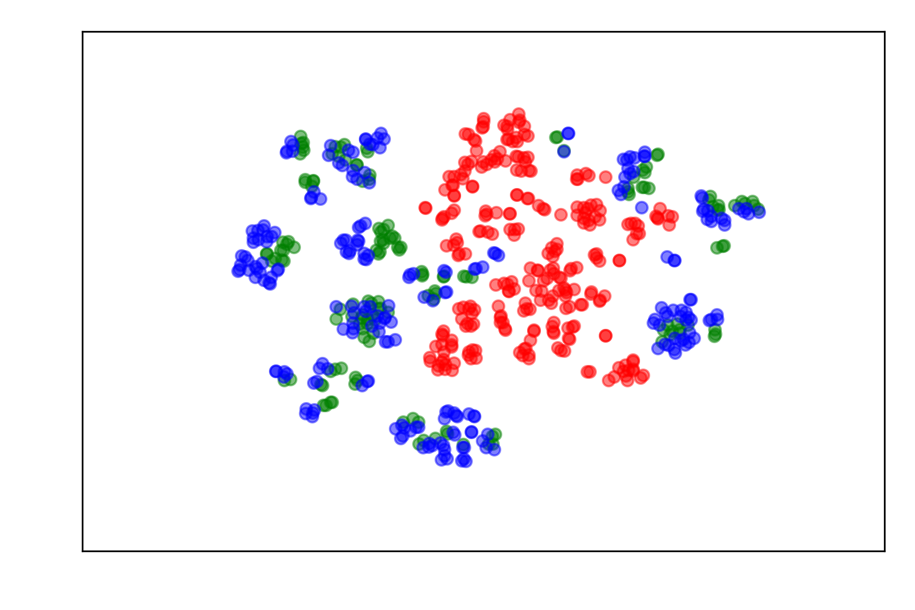
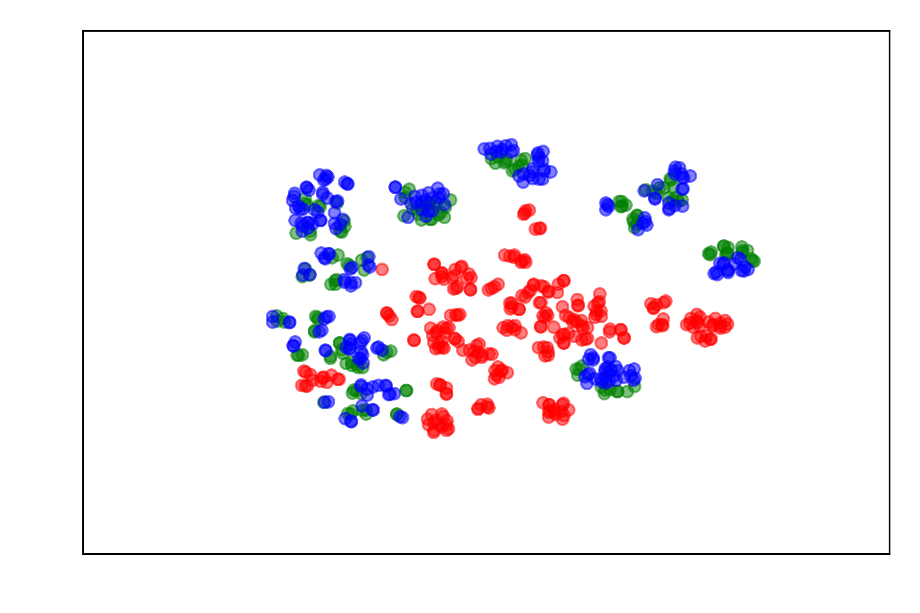
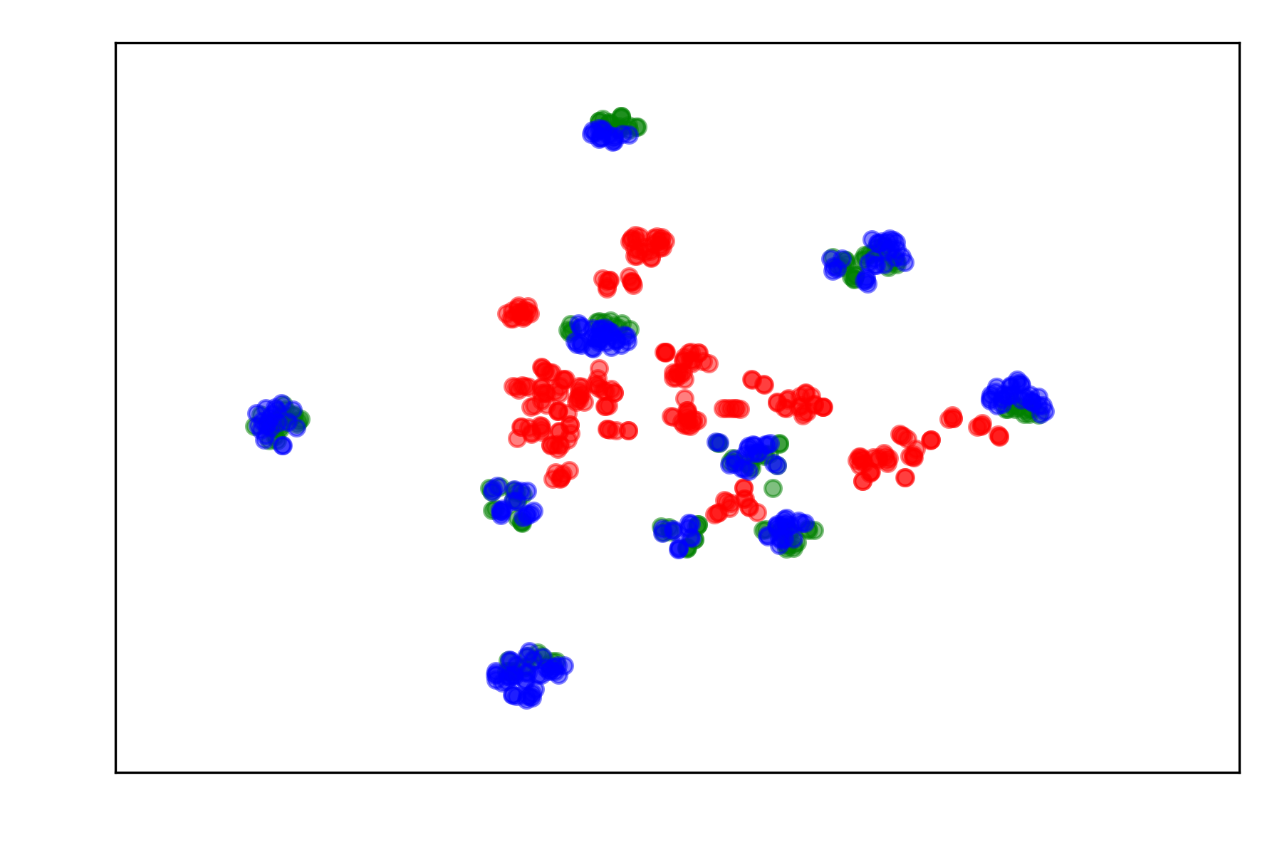
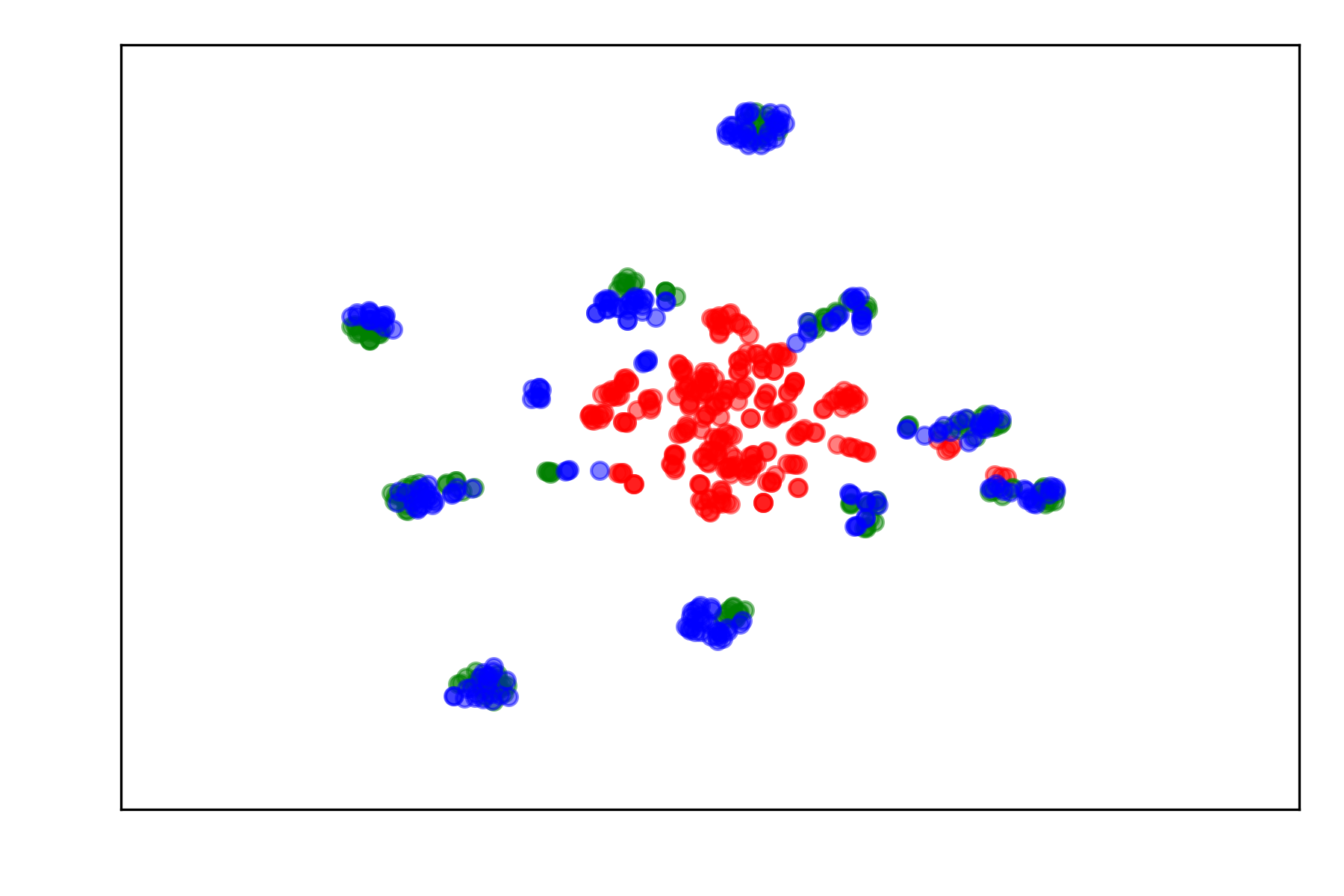
Qualitative Analysis Figure 5 represents the t-SNE visualizations [48] of the learned features by ResNet-50 (the details in Appendix C.2.3). We observe that the target-unknown (red) features from the baselines are not segregated from the source (green) and the target-known (blue) features. On the contrary, UADAL aligns the features from the source and the target-known instances accurately with clear segregation of the target-unknown features. In order to investigate the learned feature distributions quantitatively, Figure 5 provides Proxy $\mathcal{A}$-Distance (PAD) between the feature distributions from STA, ROS, and UADAL. PAD is an empirical measure of distance between domain distributions [12] (Details in Appendix C.2.4), and a higher PAD means clear discrimination between two distributions. Thus, we calculate PAD between the target-known ($tk$) and the target-unknown ($tu$) feature distributions from the feature extractor, $G$. We found that PAD from UADAL is much higher than STA and ROS. It shows that UADAL explicitly segregates the unknown features.

Figure 6: Correlation analysis between the PAD value and each of UNK (left) and HOS (right), in Office-31 dataset (with ResNet-50). The arrow represents the same task, such as A$\rightarrow$W, for UADAL and STA.

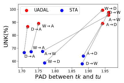
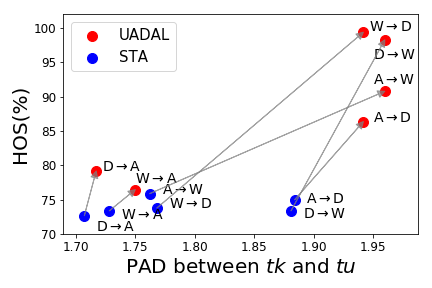
In order to provide more insights and explanations compared to STA, we provide an analysis of the correlation between the evaluation metric and the distance measure of the feature distributions. We utilize UNK, and HOS as evaluation metrics, and PAD between $tk$ and $tu$ as the distance measure. Figure 6 shows the scatter plots of (UNK & PAD) and (HOS & PAD). The grey arrows mean the corresponding tasks by UADAL and STA. As shown in the figure, HOS and UNK have a positive correlation with the distance between the target-unknown ($tu$) and the target-known ($tk$). In simple words, better segregation enables better HOS and UNK. Specifically, from STA to UADAL on the same task, the distances (PAD on $tk$/$tu$) are increased, and the corresponding performances, UNK and HOS, are also increased. It means that UADAL effectively segregates the target feature distributions, and then leads to better performance for OSDA. In other words, the proposed unknown-aware feature alignment is important to solve the OSDA problem. From this analysis, our explicit segregation of $tu$ is a key difference from the previous methods. Therefore, we claimed that this explicit segregation of UADAL is the essential part of OSDA, and leads to better performances.

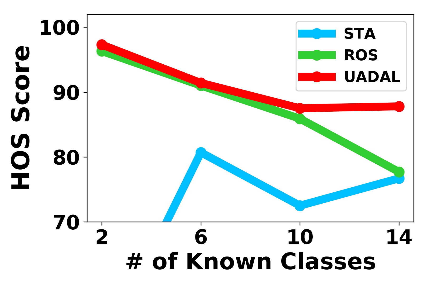
Robust on Openness We conduct the openness experiment to show the robustness of the varying number of the known classes. Figure 5 represents that UADAL performs better than the baselines over all cases. Our open-set recognition does not need to set any thresholds since we utilize the loss information of the target domain, holistically. Therefore, UADAL is robust to the degree of openness.

4.3 Ablation Studies

Effectiveness of Unknown-Aware Feature Alignment We conducted ablation studies to investigate whether the unknown-aware feature alignment is essential for the OSDA problem.

Figure 7: Convergence of Sequential Optimization.

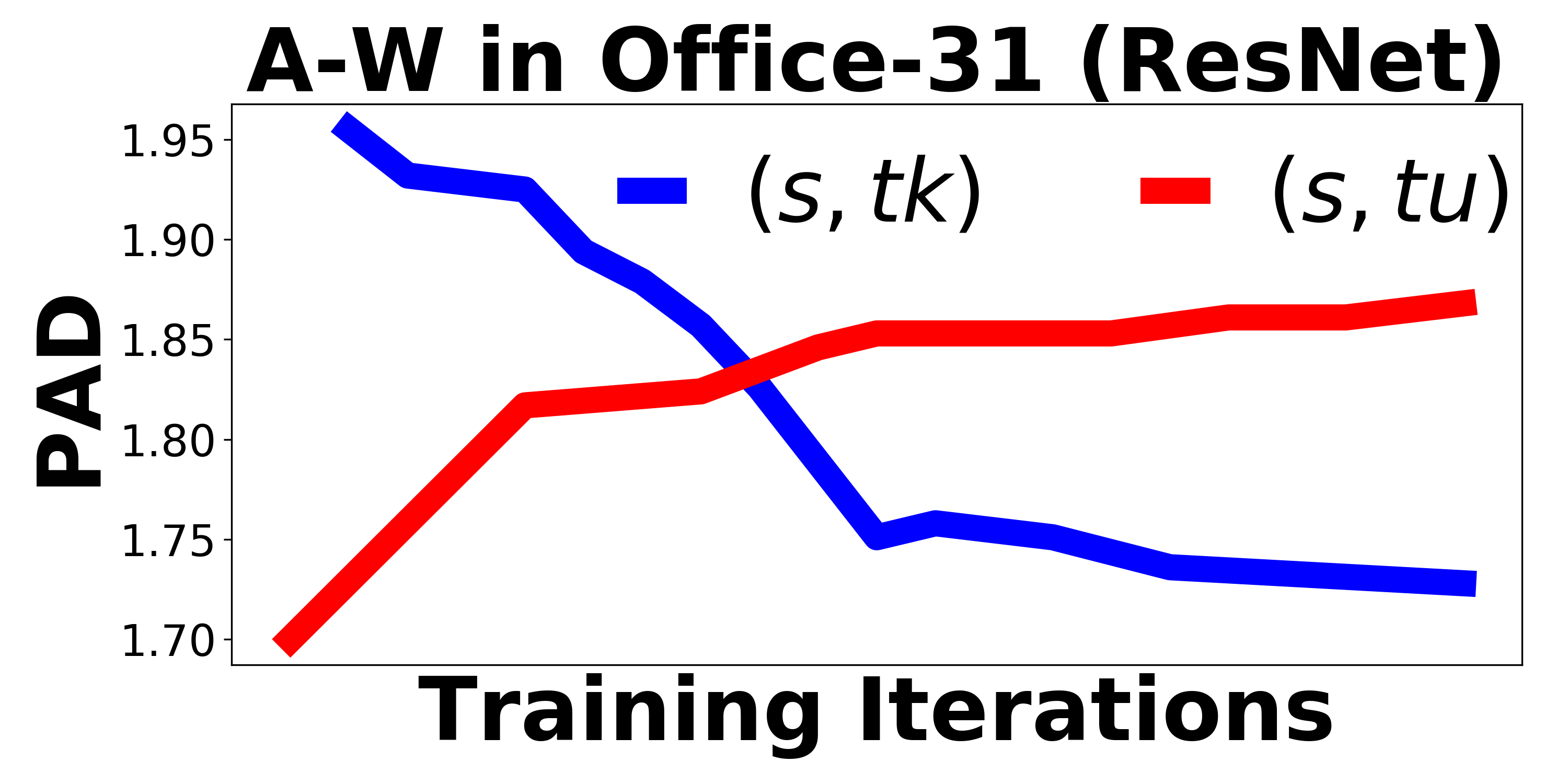
Table 3 represents the experimental results where the feature alignment procedure of STA or ROS is replaced by UADAL, maintaining their weighting schemes, in Office-31 with ResNet-50. In terms of each weighting, the UADAL core leads to better performances in both STA and ROS cases. Surprisingly, when we replace STA’s known-only matching with the unknown-aware feature alignment of UADAL, the performance increases dramatically. It means that the implicit separation of STA at the classification level is limited to segregating the target-unknown features. Therefore, explicit segregation by UADAL is an essential part to solve the OSDA problem. Moreover, Figure 7 shows the empirical convergence of the proposed sequential optimization as PAD value between $p_{s}$ and $p_{tk}$ and between $p_{s}$ and $p_{tu}$ over training, i.e., $p_{s}\approx p_{tk}$ and $p_{tu}\leftrightarrow\{p_{tk},p_{s}\}$.

(a) Early stage of training

(b) End stage of training

Figure 8: (a) The histogram of the source and target entropy with the fitted posterior inference model, at the Early / End stage of training, where the subfigure in (a) shows the histogram of $\hat{w}_{x}$ at this stage.

(a) Binary Acc.

(b) Ablation Studies

Figure 9: (a) Binary accuracy on tk/tu by thresholding $\hat{w}_{x}$. (b) Ablations for posterior inference with thresholding.

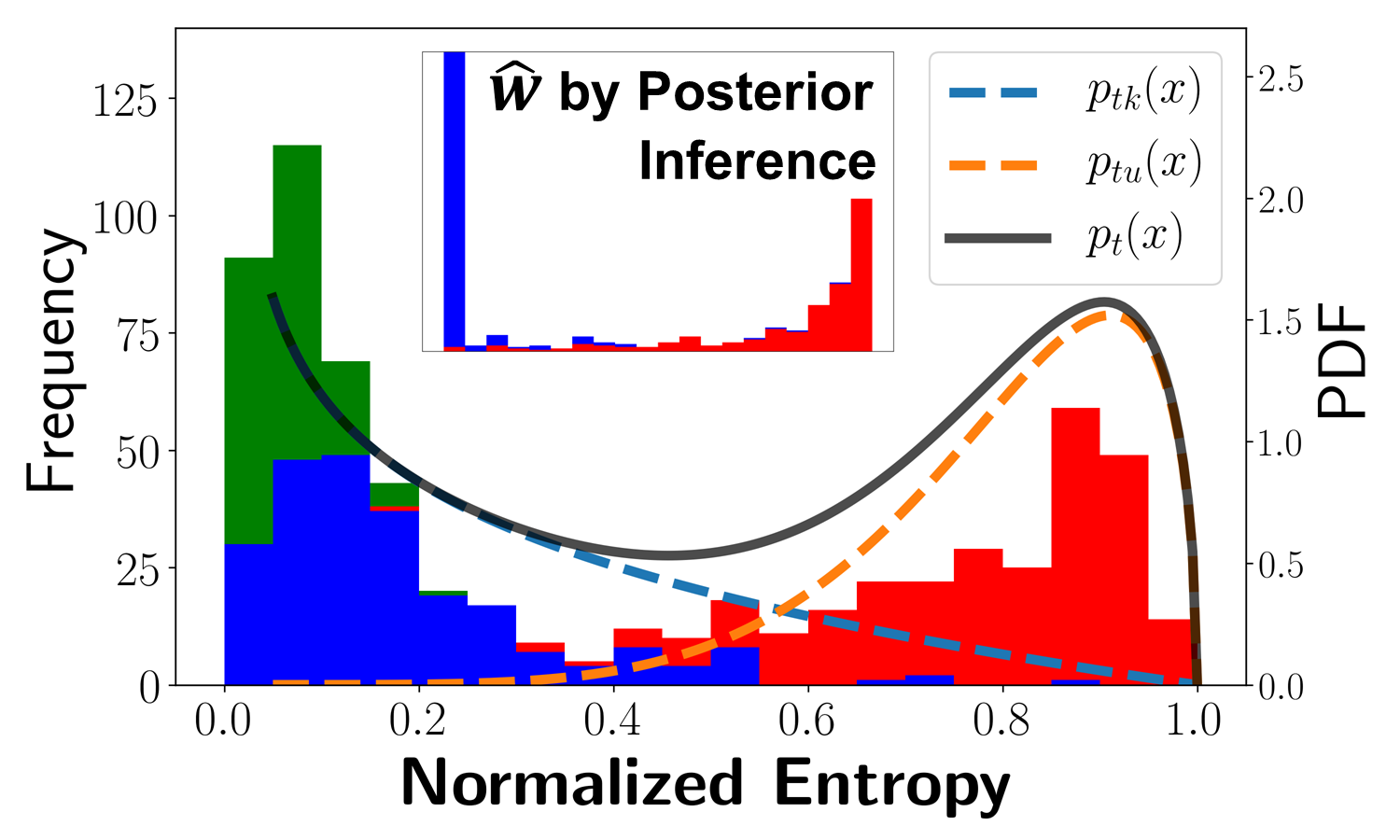
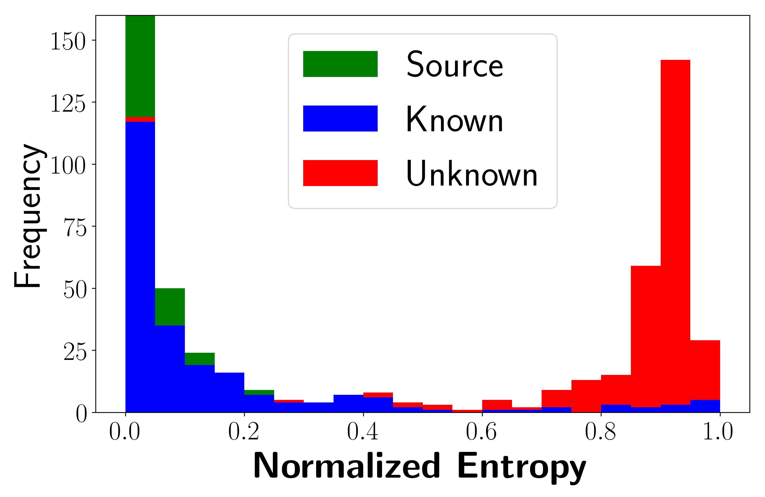
Superiorities of Open-set Recognition: (Effective Recognition) Figure 9 represents the histogram of the source/target entropy values from $E$ after the early stage of training by Eq. (20) (sensitivity analysis on the varying number of iterations for the early stage in Appendix C.2.5). Therefore, it demonstrates that our assumption on two modalities of the entropy values holds, robustly. Furthermore, the subfigure in Figure 9 shows the histogram of the $\hat{w}_{x}$ by the posterior inference. It shows that our open-set recognition, $\hat{w}_{x}$, provides a more clear separation for the target-known (blue) and the target-unknown (red) instances than the entropy values. Figure 9 represents the histogram of the entropy at the end of the training, which is further split than Figure 9. This clear separation implicitly supports that the proposed feature alignment accomplishes both alignment and segregation.

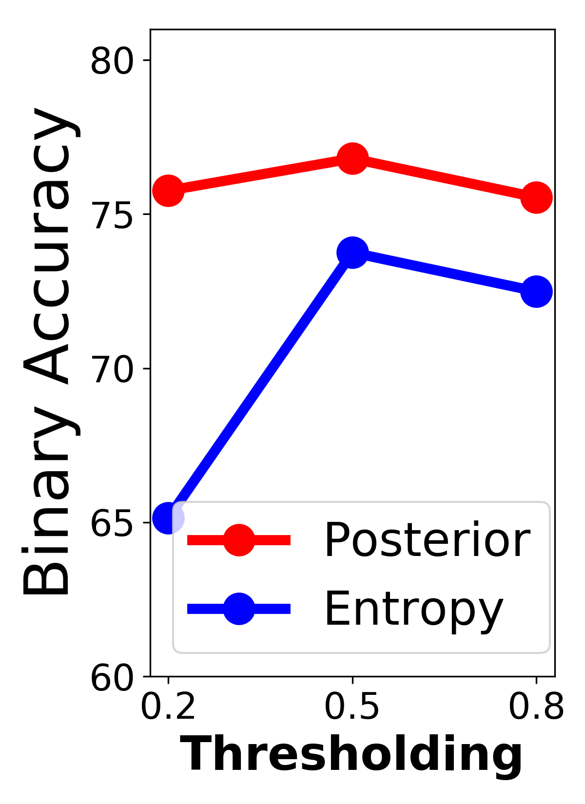
(Informativeness) Furthermore, we conduct a binary classification task by thresholding the weights, $\hat{w}_{x}$, whether it predicts $tk$ or $tu$ correctly. Figure 9 represents the accuracies over the threshold values when applying the posterior inference or the normalized entropy values themselves, in Office-31. It shows that the posterior inference discriminates $tk$ and $tu$ more correctly than using the entropy value itself. Additionally, the posterior inference has similar accuracies over the threshold values (0.2, 0.5, and 0.8), which also indicates a clear separation. Therefore, we conclude that the posterior inference provides a more informative weighting procedure than the entropy value itself.

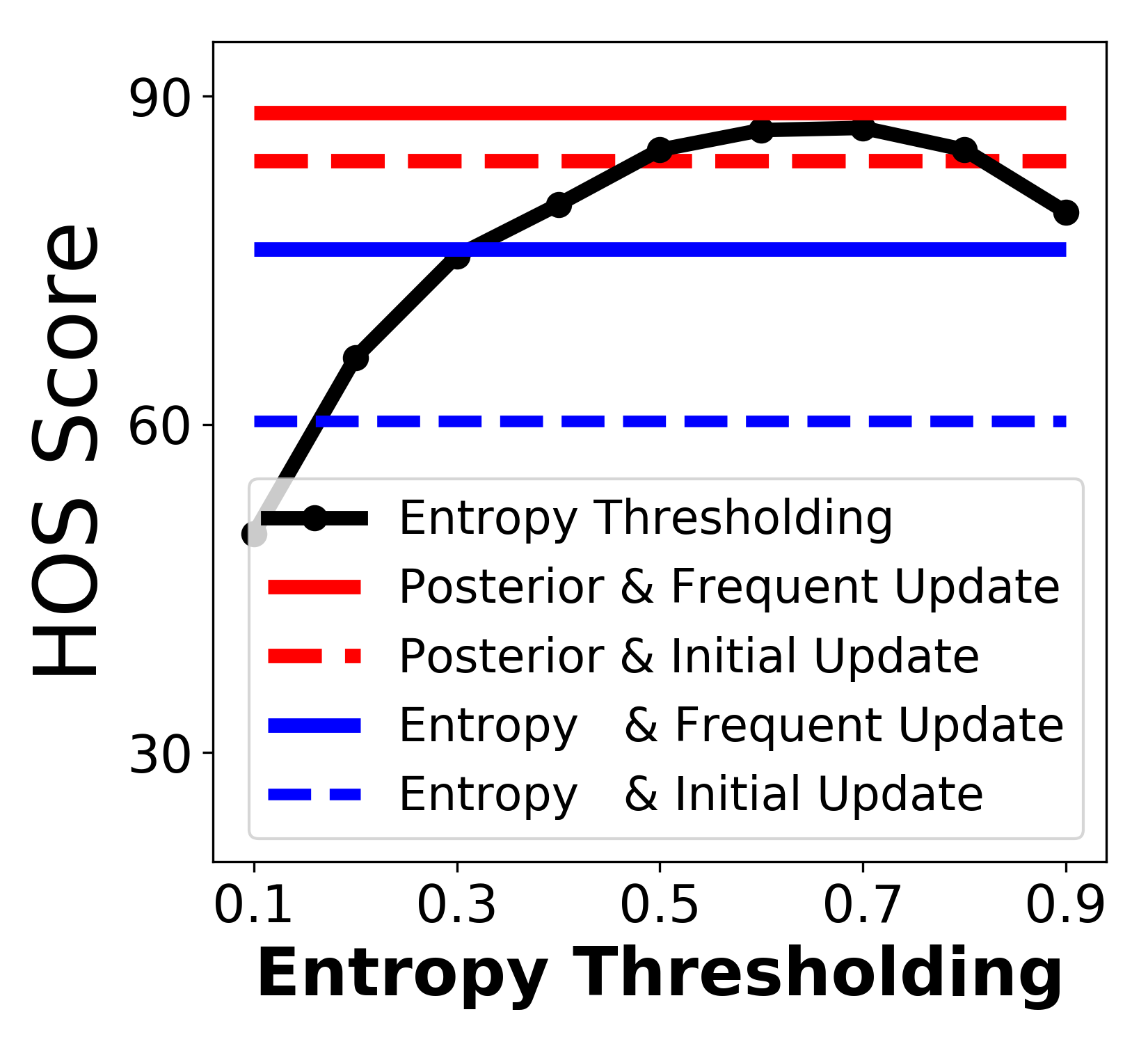
(Comparison to Thresholding) Figure 9 shows that UADAL with the posterior inference outperforms all cases of thresholding the entropy values. It means that the posterior inference is free to set thresholds. Moreover, the results demonstrate that UADAL with the posterior inference outperforms the case of using the normalized entropy value, and its frequent updating (solid line) leads to a better performance than only initial updating (dashed line). It is consistent with the analysis from Figure 9.

Figure 10: Ablation study of applying sampling on the target domain with Office-31 (left) and Office-Home (right) w.r.t. the averaged scores.

Dataset	Ent.	OS*	UNK	HOS
Office-31	X	85.4	90.0	87.5
	O	84.8	82.1	88.1
Office-Home	X	61.9	75.2	67.6
	O	62.6	78.0	68.7

Table 4: Ablation on Entropy Minimization (Ent.) Loss from Eq. (19) on the Office-31 and Office-Home. The values in the table are the averaged score over the tasks in each dataset. The detailed results are in Table 6 in Appendix C.2.7.

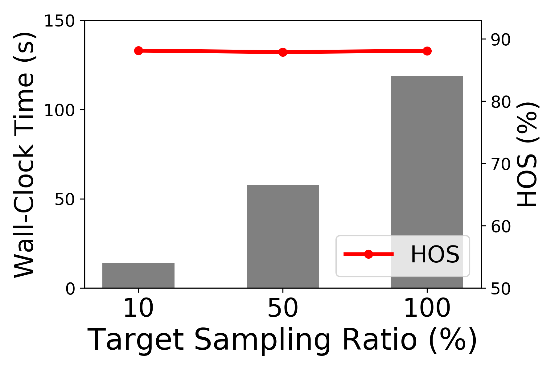
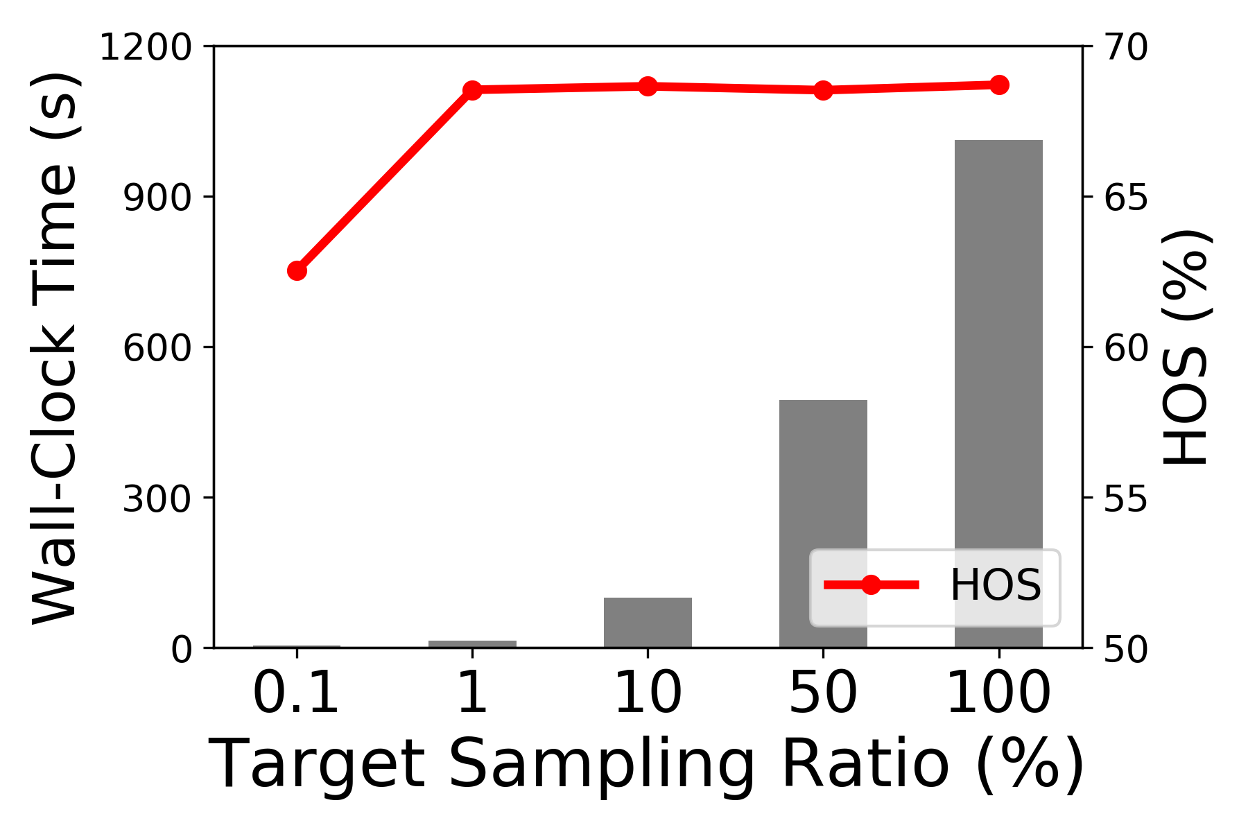
(Efficiency) In terms of computation, the posterior inference increases the complexity because we need to fit the mixture model, where the computational complexity is $O(nk)$ with the number of samples, $n$, and the number of fitting iterations, $k$ ($n\gg k$). As an alternative, we fit the mixture model only by sampling the target instance. Figure 10 represents the wall-clock time increased by the fitting process and the performances over the sampling ratio (%) for the target domain. Since the computational complexity is linearly increased by the number of samples, the wall-clock time is also linearly increased by increasing the sampling ratio. Interestingly, we observed that even when the sampling ratio is small, i.e. 10%, the performances do not decrease, on both Office-31 and Office-Home datasets. The qualitative analysis of this sampling is provided in Appendix C.2.8.

Entropy Minimization Loss In order to show the effect of the entropy minimization by Eq. (19), we conduct the ablation study on the Office-31 and Office-Home. Table 4 shows that the entropy minimization leads to better performance. However, UADAL without the loss still performs better than the other baselines (compared with Table 1). It represents that UADAL learns the feature space appropriately as we intended to suit Open-Set Domain Adaptation. The properly learned feature space leads to effectively classifying the target instances without entropy minimization.

5 Conclusion

We propose Unknown-Aware Domain Adversarial Learning (UADAL), which is the first approach to explicitly design the segregation of the unknown features in the domain adversarial learning for OSDA. We design a new domain discrimination loss and formulate the sequential optimization for the unknown-aware feature alignment. Empirically, UADAL outperforms all baselines on all benchmark datasets with various backbone networks, by reporting state-of-the-art performances.

Checklist

1. For all authors…

   1. Do the main claims made in the abstract and introduction accurately reflect the paper’s contributions and scope? [Yes]

   2. Did you describe the limitations of your work? [Yes] Details in Appendix D.

   3. Did you discuss any potential negative societal impacts of your work? [Yes] Details in Appendix D.

   4. Have you read the ethics review guidelines and ensured that your paper conforms to them? [Yes]

2. If you are including theoretical results…

   1. Did you state the full set of assumptions of all theoretical results? [Yes]

   2. Did you include complete proofs of all theoretical results? [Yes]

3. If you ran experiments…

   1. Did you include the code, data, and instructions needed to reproduce the main experimental results (either in the supplemental material or as a URL)? [Yes] We provide code in supplemental material, and URL of data and instructions are provided in Appendix C.1.5.

   2. Did you specify all the training details (e.g., data splits, hyperparameters, how they were chosen)? [Yes]

   3. Did you report error bars (e.g., with respect to the random seed after running experiments multiple times)? [Yes]

   4. Did you include the total amount of compute and the type of resources used (e.g., type of GPUs, internal cluster, or cloud provider)? [Yes] The details in Appendix C.1.1.

4. If you are using existing assets (e.g., code, data, models) or curating/releasing new assets…

   1. If your work uses existing assets, did you cite the creators? [Yes]

   2. Did you mention the license of the assets? [Yes]

   3. Did you include any new assets either in the supplemental material or as a URL? [Yes] See Appendix C.1.4 and C.1.5.

   4. Did you discuss whether and how consent was obtained from people whose data you’re using/curating? [Yes] We mentioned that we use the public benchmark dataset, in Section 4.1.

   5. Did you discuss whether the data you are using/curating contains personally identifiable information or offensive content? [Yes] We use image object recognition datasets, so there are no personaly identifiable information or offensive content.

5. If you used crowdsourcing or conducted research with human subjects…

   1. Did you include the full text of instructions given to participants and screenshots, if applicable? [N/A]

   2. Did you describe any potential participant risks, with links to Institutional Review Board (IRB) approvals, if applicable? [N/A]

   3. Did you include the estimated hourly wage paid to participants and the total amount spent on participant compensation? [N/A]

This is an Appendix for "Unknown-Aware Domain Adversarial Learning for Open-Set Domain Adaptation". First, Section A provides comprehensive literature reviews. Second, Section B provides the details for the proposed model, UADAL. It consists of three parts; 1) Sequential Optimization Problem (Section B.1), 2) Posterior Inference (Section B.2), and 3) Training Details (Section B.3). Third, Section C provides the experimental details, including the implementation details (Section C.1) and the detailed experimental results (Section C.2). Finally, Section D shows ‘Limitations and Potential Negative Societal Impacts’ of this work.

Note that all references and the equation numbers are independent of the main paper. We utilize the expression of "Eq. (XX) in the main paper", especially when referring the equations from the main paper.

Appendix A Literature Reviews

(Closed-Set) Domain Adaptation (DA) is the task of leveraging the knowledge of the labeled source domain to the target domain [5, 3, 2, 23, 12]. Here, DA assumes that the class sets from the source and the target domain are identical. The typical approaches to solve DA have focused on minimizing the discrepancy between the source and the target domain since they are assumed to be drawn from the different distributions [33, 46, 24, 25]. The discrepancy-based approaches have been proposed to define the metric to measure the distance between the source and the target domain in the feature space [23, 53]. Other works are based on adversarial methods [11, 47, 27]. These approaches introduce the domain discriminator and a feature generator in order to learn the feature space to be domain-invariant. Self-training methods are also proposed to mitigate the DA problems by pseudo-labeling the target instances [22, 19, 30, 35], originally tailored to semi-supervised learning [14, 43].

Open-Set Recognition (OSR) is the task to classify an instance correctly if it belongs to the known classes or to reject outliers otherwise, during the testing phase [39]. Here, the outliers are called ‘open-set’ which is not available in the training phase. Many approaches have been proposed to solve the OSR problem [4, 31, 44, 32, 40, 7, 8]. OpenMax [4] is the first deep learning approach for OSR, introducing a new model layer to estimate the probability of an instance being unknown class, based on the Extreme Value Theory (EVT). OSRCI [31], another stream of the approaches utilizing GANs, generates the virtual images which are similar to the training instances but do not belong to the known classes. Other approaches contain the reconstruction-based methods [44, 32] and prototype-based methods [40, 7, 8]. Also, [49] claims that the performance of OSR is highly correlated with its accuracy on the closed-set classes. This claim is associated with our open-set recognizer.

Open-Set Domain Adaptation is a more realistic and challenging task of Domain Adaptation, where the target domain includes the open-set instances which are not discovered by the source domain. In terms of the domain adversarial learning, in addition to STA, OSBP [37] utilizes a classifier to predict the target instances to the pre-determined threshold, and trains the feature extractor to deceive the classifier for aligning to known classes or rejecting as unknown class. However, their recognition on unknown class only depends on the threshold value, without considering the data instances. PGL [29] introduces progressive graph-based learning to regularize the class-specific manifold, while jointly optimizing with domain adversarial learning. However, their adversarial loss includes all instances of the target domain, which is critically weakened by the negative transfer.

In terms of the self-supervised learning, ROS [6] is rotation-based self-supervised learning to compute the normality score for separating target known/unknown information. DANCE [38] is based on a self-supervised clustering to move a target instance either to shared-known prototypes in the source domain or to its neighbor in the target domain. DCC [20] is a domain consensus clustering to exploit the intrinsic structure of the target domain. However, these approaches do not have any feature alignments between the source and the target domain, which leads to performance degradation under the significant domain shifts.

There is also a notable work, OSLPP [51] optimizing projection matrix toward a common subspace to class-wisely align the source and the target domain. This class-wise matching depends on the pseudo label for the target instances. However, inaccurate pseudo labels such as early mistakes can result in error accumulation and domain misalignment [35]. Moreover, the optimization requires the pair-wise distance calculation, which results in a growing complexity of $O(n^{2})$ by the $n$ data instances. It could be limited to the large-scaled domain.

Appendix B Algorithm and Optimization Details

B.1 Sequential Optimization Problem

B.1.1 Decomposition of Domain Discrimination Loss

The domain discrimination loss for the target domain is as below, (Eq. (7) in the main paper)

$$\mathcal{L}_{d}^{t}(\theta_{g},\theta_{d})=\mathbb{E}_{p_{t}(x)}[\ -w_{x}\log D_{tk}(G(x))-(1-w_{x})\log D_{tu}(G(x))],$$

where $w_{x}=p(known|x)$ is the probability of a target instance, $x$, belonging to a target-known class. Then, we decompose $\mathcal{L}_{d}^{t}(\theta_{g},\theta_{d})$ into the two terms, $\mathcal{L}_{d}^{tk}(\theta_{g},\theta_{d})$ and $\mathcal{L}_{d}^{tu}(\theta_{g},\theta_{d})$, as follows,

$$\mathcal{L}_{d}^{t}(\theta_{g},\theta_{d}) =\mathcal{L}_{d}^{tk}(\theta_{g},\theta_{d})+\mathcal{L}_{d}^{tu}(\theta_{g},\theta_{d}),$$

$$\mathcal{L}_{d}^{tk}(\theta_{g},\theta_{d}) :=\lambda_{tk}\cdot\mathbb{E}_{p_{tk}(x)}\left[-\log D_{tk}(G(x))\right],$$

$$\mathcal{L}_{d}^{tu}(\theta_{g},\theta_{d}) :=\lambda_{tu}\cdot\mathbb{E}_{p_{tu}(x)}\left[-\log D_{tu}(G(x))\right],$$

where $p_{tk}(x):=p_{t}(x|known)$ and $p_{tu}(x):=p_{t}(x|unknown)$; $\lambda_{tk}=p(known)$; and $\lambda_{tu}=p(unknown)$.

Proof.

We start this proof from Eq. (7) in the main paper,

$$\mathcal{L}_{d}^{t}(\theta_{g},\theta_{d})= \ \mathbb{E}_{p_{t}(x)}[\ -w_{x}\log D_{tk}(G(x))-(1-w_{x})\log D_{tu}(G(x))].$$

For the convenience of the derivation, we replace $w_{x}$ as $p(known|x)$.

$$\mathcal{L}_{d}^{t} (\theta_{g},\theta_{d})=\mathbb{E}_{x\sim p_{t}(x)}\left[\ -p_{t}(known|x)\log D_{tk}(G(x))-p_{t}(unknown|x)\log D_{tu}(G(x))\right]$$

$$=\int\limits_{x\sim p_{t}(x)}\Big{(}-p_{t}(known|x)\log D_{tk}(G(x))-p_{t}(unknown|x)\log D_{tu}(G(x))\Big{)}\,dx$$

$$=\int\limits_{x}\Big{(}-p_{t}(x)(p_{t}(known|x)\log D_{tk}(G(x))-p_{t}(x)p_{t}(unknown|x)\log D_{tu}(G(x))\Big{)}\,dx$$

$$=\int\limits_{x}\Big{(}-p_{t}(known,x)\log D_{tk}(G(x))-p_{t}(unknown,x)\log D_{tu}(G(x))\Big{)}\,dx$$

$$=\int\limits_{x}-p_{t}(x|known)p_{t}(known)\log D_{tk}(G(x))\,dx+\int\limits_{x}-p_{t}(x|unknown)p_{t}(unknown)\log D_{tu}(G(x))\,dx$$

$$=p_{t}(known)\int\limits_{x}-p_{t}(x|known)\log D_{tk}(G(x))\,dx+p_{t}(unknown)\int\limits_{x}-p_{t}(x|unknown)\log D_{tu}(G(x))\,dx$$

$$=p_{t}(known)\int\limits_{x\sim p_{tk}(x)}-\log D_{tk}(G(x))\,dx+p_{t}(unknown)\int\limits_{x\sim p_{tu}(x)}-\log D_{tu}(G(x))\,dx$$

$$=p_{t}(known)\mathbb{E}_{x\sim p_{tk}(x)}\left[-\log D_{tk}(G(x))\right]+p_{t}(unknown)\mathbb{E}_{x\sim p_{tu}(x)}\left[-\log D_{tu}(G(x))\right]$$

$$=\lambda_{tk}\mathbb{E}_{x\sim p_{tk}(x)}\left[-\log D_{tk}(G(x))\right]+\lambda_{tu}\mathbb{E}_{x\sim p_{tu}(x)}\left[-\log D_{tu}(G(x))\right].$$

Thus, we define new terms with respect to $p_{tk}(x)$ and $p_{tu}(x)$ as follow.

$$\mathcal{L}_{d}^{tk}(\theta_{g},\theta_{d}) :=\lambda_{tk}\mathbb{E}_{x\sim p_{tk}(x)}\left[-\log D_{tk}(G(x))\right]$$

$$\mathcal{L}_{d}^{tu}(\theta_{g},\theta_{d}) :=\lambda_{tu}\mathbb{E}_{x\sim p_{tu}(x)}\left[-\log D_{tu}(G(x))\right]$$

Therefore, by the above derivation, we decompose $\mathcal{L}_{d}^{t}(\theta_{g},\theta_{d})$ as follow,

$$\mathcal{L}_{d}^{t}(\theta_{g},\theta_{d})=\mathcal{L}_{d}^{tk}(\theta_{g},\theta_{d})+\mathcal{L}_{d}^{tu}(\theta_{g},\theta_{d}).$$

∎

B.1.2 Optimal point of the domain discriminator $D$

The optimal $D^{*}$ given the fixed $G$ is as follow (Eq. (13) in the main paper),

$$D^{*}(G(x;\theta_{g}))=D^{*}(z)=\Big{[}\frac{p_{s}(z)}{2p_{avg}(z)},\frac{\lambda_{tk}p_{tk}(z)}{2p_{avg}(z)},\frac{\lambda_{tu}p_{tu}(z)}{2p_{avg}(z)}\Big{]},$$

where $p_{avg}(z)=(p_{s}(z)+\lambda_{tk}p_{tk}(z)+\lambda_{tu}p_{tu}(z))/2$. Note that $z\in\mathcal{Z}$ stands for the feature space from $G$. In other words, $p_{d}(z)=\{G(x;\theta_{g})|x\sim p_{d}(x)\}$ where $d$ is $s$, $tk$, or $tu$.

Proof.

First, we fix $G$, and optimize the problem with respect to $D$.

$$\min_{\theta_{d}}\ \mathcal{L}_{D}(\theta_{g},\theta_{d})=\mathcal{L}_{d}^{s}(\theta_{g},\theta_{d})+\ \mathcal{L}_{d}^{tk}(\theta_{g},\theta_{d})+\mathcal{L}_{d}^{tu}(\theta_{g},\theta_{d})$$

$$=-\int\limits_{x\sim p_{s}(x)}\log D_{s}(G(x))\,dx-\lambda_{tk}\int\limits_{x\sim p_{tk}(x)}\log D_{tk}(G(x))\,dx-\lambda_{tu}\int\limits_{x\sim p_{tu}(x)}\log D_{tu}(G(x))\,dx$$

$$=-\int\limits_{z\sim p_{s}(z)}\log D_{s}(z)\,dz-\lambda_{tk}\int\limits_{z\sim p_{tk}(z)}\log D_{tk}(z)\,dz-\lambda_{tu}\int\limits_{x\sim p_{tu}(z)}\log D_{tu}(z)\,dz$$

$$=\int_{z}\Big{(}-p_{s}(z)\log D_{s}(z)-\lambda_{tk}p_{tk}(z)\log D_{tk}(z)-\lambda_{tu}p_{tu}(z)\log D_{tu}(z)\Big{)}\,dz$$

Also, note that $D_{s}(z)+D_{tk}(z)+D_{tu}(z)=1$ for all $z$. Therefore, we transform the optimization problem as follow [13]:

$$\min_{\theta_{d}} \quad-p_{s}(z)\log D_{s}(z)-\lambda_{tk}p_{tk}(z)\log D_{tk}(z)-\lambda_{tu}p_{tu}(z)\log D_{tu}(z)$$

s.t. $$\quad D_{s}(z)+D_{tk}(z)+D_{tu}(z)=1$$

for all $z$. We introduce the Lagrange variable $v$ to use Lagrange multiplier method.

$$\begin{split}\min_{\theta_{d}}\mathcal{\tilde{L}}_{D}:=&-p_{s}(z)\log D_{s}(z)-\lambda_{tk}p_{tk}(z)\log D_{tk}(z)-\lambda_{tu}p_{tu}(z)\log D_{tu}(z)\\ &\quad+v(D_{s}(z)+D_{tk}(z)+D_{tu}(z)-1)\\ \end{split}$$

To find optimal $D^{*}$, we find the derivative of $\mathcal{\tilde{L}}_{D}$ with respect to $D$ and $v$.

$$\frac{\partial\mathcal{\tilde{L}}_{D}}{\partial D_{s}(z)}=\frac{-p_{s}(z)}{D_{s}(z)}+v=0\quad\Leftrightarrow\quad D_{s}(z)=\frac{p_{s}(z)}{v}$$

$$\frac{\partial\mathcal{\tilde{L}}_{D}}{\partial D_{tk}(z)}=\frac{-\lambda_{tk}p_{tk}(z)}{D_{tk}(z)}+v=0\quad\Leftrightarrow\quad D_{tk}(z)=\frac{\lambda_{tk}p_{tk}(z)}{v}$$

$$\frac{\partial\mathcal{\tilde{L}}_{D}}{\partial D_{tu}(z)}=\frac{-\lambda_{tu}p_{tu}(z)}{D_{tu}(z)}+v=0\quad\Leftrightarrow\quad D_{tu}(z)=\frac{\lambda_{tu}p_{tu}(z)}{v}$$

$$\frac{\partial\mathcal{\tilde{L}}_{D}}{\partial v}=D_{s}(z)+D_{tk}(z)+D_{tu}(z)-1=0\quad\Leftrightarrow\quad D_{s}(z)+D_{tk}(z)+D_{tu}(z)=1$$

From the above equations, we have

$$D_{s}(z)+D_{tk}(z)+D_{tu}(z)=\frac{p_{s}(z)}{v}+\frac{\lambda_{tk}p_{tk}(z)}{v}+\frac{\lambda_{tu}p_{tu}(z)}{v}=1,$$

then,

$$v=p_{s}(z)+\lambda_{tk}p_{tk}(z)+\lambda_{tu}p_{tu}(z)=2p_{avg}(z).$$

Thus, we get optimal $D^{*}$ as

$$D^{*}(z)=[D_{s}^{*}(z),D_{tk}^{*}(z),D_{tu}^{*}(z)]=\Big{[}\frac{p_{s}(z)}{2p_{avg}(z)},\frac{\lambda_{tk}p_{tk}(z)}{2p_{avg}(z)},\frac{\lambda_{tu}p_{tu}(z)}{2p_{avg}(z)}\Big{]}.$$

∎

B.1.3 Proof of Theorem 14

Theorem B.1.

Let $\theta^{*}_{d}$ be the optimal parameter of $D$ by optimizing Eq. (11) in the main paper. Then, $-\mathcal{L}_{G}(\theta_{g},\theta^{*}_{d})$ can be expressed as, with a constant $C_{0}$,

$$-\mathcal{L}_{G}(\theta_{g}, \theta^{*}_{d})=D_{KL}(p_{s}\|p_{avg})+\lambda_{tk}D_{KL}(p_{tk}\|p_{avg})-\lambda_{tu}D_{KL}(p_{tu}\|p_{avg})+C_{0}.$$

Proof.

First, we change maximization problem into minimization problem, and substitute $D^{*}$ by using Eq. (13) in the main paper. Note that $p_{avg}=(p_{s}(z)+\lambda_{tk}p_{tk}(z)+\lambda_{tu}p_{tu}(z))/2$.

$$\min_{\theta_{g}}\ - \mathcal{L}_{G}(\theta_{g},\theta_{d})=-\mathcal{L}_{d}^{s}(\theta_{g},\theta_{d})-\ \mathcal{L}_{d}^{tk}(\theta_{g},\theta_{d})+\mathcal{L}_{d}^{tu}(\theta_{g},\theta_{d})$$ (23)

$$=\int_{z}\left(p_{s}(z)\log D_{s}^{*}(z)+\lambda_{tk}p_{tk}(z)\log D_{tk}^{*}(z)-\lambda_{tu}p_{tu}(z)\log D_{tu}^{*}(z)\right)\,dz$$ (24)

$$=\int_{z}(\ p_{s}(z)\log{\frac{p_{s}(z)}{2p_{avg}(z)}}+\lambda_{tk}p_{tk}(z)\log{\frac{\lambda_{tk}p_{tk}(z)}{2p_{avg}(z)}}-\lambda_{tu}p_{tu}(z)\log{\frac{\lambda_{tu}p_{tu}(z)}{2p_{avg}(z)}}\ )\,dz$$ (25)

$$=D_{KL}(p_{s}\|p_{avg})+\lambda_{tk}D_{KL}(p_{tk}\|p_{avg})-\lambda_{tu}D_{KL}(p_{tu}\|p_{avg})+C_{0}$$ (26)

where $C_{0}=-2\lambda_{tk}\log 2+\lambda_{tk}\log\lambda_{tk}-\lambda_{tu}\log\lambda_{tu}$.

We use below derivation for the last equation, i.e. from Eq. (25) to Eq. (26).

$$D_{KL}(p_{s}\|p_{avg}) =\int_{z}p_{s}(z)\log{\frac{p_{s}(z)}{(p_{avg}(z)}}\,dz$$

$$=\int_{z}p_{s}(z)\log{\frac{2p_{s}(z)}{p_{s}(z)+\lambda_{tk}p_{tk}(z)+\lambda_{tu}p_{tu}(z)}}\,dz$$

$$=\int_{z}p_{s}(z)\log{\frac{p_{s}(z)}{p_{s}(z)+\lambda_{tk}p_{tk}(z)+\lambda_{tu}p_{tu}(z)}}\,dz$$

$$\quad\quad+\int_{z}p_{s}(z)\log{2}\,dz$$

$$=\int_{z}p_{s}(z)\log{\frac{p_{s}(z)}{2p_{avg}(z)}}\,dz+\int_{z}p_{s}(z)\log{2}\,dz$$

Thus,

$$\int_{z}p_{s}(z)\log{\frac{p_{s}(z)}{2p_{avg}(z)}}\,dz=D_{KL}(p_{s}\|p_{avg})-\log{2}$$ (27)

For the second term,

$$D_{KL}(p_{tk}\|p_{avg})$$

$$=\int_{z}p_{tk}(z)\log{\frac{p_{tk}(z)}{p_{avg}(z)}}\,dz$$

$$=\int_{z}p_{tk}(z)\log{\frac{2p_{tk}(z)}{p_{s}(z)+\lambda_{tk}p_{tk}(z)+\lambda_{tu}p_{tu}(z)}}\,dz$$

$$=\int_{z}p_{tk}(z)\log{\frac{p_{tk}(z)}{p_{s}(z)+\lambda_{tk}p_{tk}(z)+\lambda_{tu}p_{tu}(z)}}\,dz+\int_{z}p_{tk}(z)\log{2}\,dz$$

$$=\int_{z}p_{tk}(z)\log{\frac{p_{tk}(z)}{p_{s}(z)+\lambda_{tk}p_{tk}(z)+\lambda_{tu}p_{tu}(z)}}\,dz+\log{2}$$

$$=\int_{z}p_{tk}(z)(\log{\frac{p_{tk}(z)}{p_{s}(z)+\lambda_{tk}p_{tk}(z)+\lambda_{tu}p_{tu}(z)}}+\log\lambda_{tk}-\log\lambda_{tk})\,dz+\log{2}$$

$$=\int_{z}p_{tk}(z)\log{\frac{\lambda_{tk}p_{tk}(z)}{p_{s}(z)+\lambda_{tk}p_{tk}(z)+\lambda_{tu}p_{tu}(z)}}\,dz-\log\lambda_{tk}+\log{2}$$

$$=\int_{z}p_{tk}(z)\log{\frac{\lambda_{tk}p_{tk}(z)}{2p_{avg}(z)}}\,dz-\log\lambda_{tk}+\log{2}$$

By multiplying $\lambda_{tk}$,

$$\lambda_{tk}D_{KL}(p_{tk}\|p_{avg}) =\int_{z}\lambda_{tk}p_{tk}(z)\log{\frac{\lambda_{tk}p_{tk}(z)}{2p_{avg}(z)}}\,dz-\lambda_{tk}\log{\frac{\lambda_{tk}}{2}}$$

Thus,

$$\int_{z}\lambda_{tk}p_{tk}(z)\log{\frac{\lambda_{tk}p_{tk}(z)}{2p_{avg}(z)}}\,dz =\lambda_{tk}D_{KL}(p_{tk}\|p_{avg})+\lambda_{tk}\log{\frac{\lambda_{tk}}{2}}$$ (28)

Similarly, for the third term,

$$\int_{z}\lambda_{tu}p_{tu}(z)\log{\frac{\lambda_{tu}p_{tu}(z)}{2p_{avg}(z)}}\,dz =\lambda_{tu}D_{KL}(p_{tu}\|p_{avg})+\lambda_{tu}\log{\frac{\lambda_{tu}}{2}}$$ (29)

In summary, from the Eq. (27), (28), and (29), we obtain the minimization problem with respect to $G$ as follows,

$$\begin{split}\min_{\theta_{g}}\ -\mathcal{L}_{G}(\theta_{g},\theta_{d})&=-\mathcal{L}_{d}^{s}(\theta_{g},\theta_{d})-\ \mathcal{L}_{d}^{tk}(\theta_{g},\theta_{d})+\mathcal{L}_{d}^{tu}(\theta_{g},\theta_{d})\\ &=D_{KL}(p_{s}\|p_{avg})+\lambda_{tk}D_{KL}(p_{tk}\|p_{avg})-\lambda_{tu}D_{KL}(p_{tu}\|p_{avg})+C_{0},\end{split}$$ (30)

where $C_{0}=-\log{2}+\lambda_{tk}\log{\frac{\lambda_{tk}}{2}}-\lambda_{tu}\log{\frac{\lambda_{tu}}{2}}=-2\lambda_{tk}\log 2+\lambda_{tk}\log\lambda_{tk}-\lambda_{tu}\log\lambda_{tu}$. ∎

B.1.4 Proof of Proposition 3.2

Proposition B.2.

The third term of the right-hand side in Eq. (14) in the main paper, $D_{KL}(p_{tu}\|p_{avg})$, is bounded to $\log 2-\log{\lambda_{tu}}$ .

Proof.

$$D_{KL}(p_{tu}\|p_{avg})=\int_{z}p_{tu}(z)\log{\frac{p_{tu}(z)}{p_{avg}(z)}}\,dz$$

$$=\int_{z}p_{tu}(z)\log{\frac{2p_{tu}(z)}{p_{s}(z)+\lambda_{tk}p_{tk}(z)+\lambda_{tu}p_{tu}(z)}}\,dz$$

$$=\int_{z}p_{tu}(z)\log{2}\,dz+\int_{z}p_{tu}(z)\log{\frac{p_{tu}(z)}{p_{s}(z)+\lambda_{tk}p_{tk}(z)+\lambda_{tu}p_{tu}(z)}}\,dz$$

$$=\log{2}+\int_{z}p_{tu}(z)\log{p_{tu}(z)}\,dz-\int_{z}p_{tu}(z)\log{(p_{s}(z)+\lambda_{tk}p_{tk}(z)+\lambda_{tu}p_{tu}(z))}\,dz$$

$$\leq\log{2}+\int_{z}p_{tu}(z)\log{p_{tu}(z)}\,dz-\int_{z}p_{tu}(z)\log{\lambda_{tu}p_{tu}(z)}\,dz$$

$$\quad(\ p_{s}(z)+\lambda_{k}p_{tk}(z)+\lambda_{tu}p_{tu}(z)\geq\lambda_{tu}p_{tu}(z)\text{ for all }z)$$

$$=\log{2}+\int_{z}p_{tu}(z)\log{p_{tu}(z)}\,dz-\int_{z}p_{tu}(z)\log{p_{tu}(z)}\,dz-\int_{z}p_{tu}(z)\log{\lambda_{tu}}\,dz$$

$$=\log{2}-\log{\lambda_{tu}}$$

Therefore,

$$D_{KL}(p_{tu}\|p_{avg})\leq\log{2}-\log{\lambda_{tu}}.$$

∎

B.1.5 Proof of Proposition 3.3

Proposition B.3.

Assume that $\text{supp}(p_{s})\cap\text{supp}(p_{tu})=\emptyset$ and $\text{supp}(p_{tk})\cap\text{supp}(p_{tu})=\emptyset$, where $\text{supp}(p):=\{z\in\mathcal{Z}|p(z)>0\}$ is the support set of probability distribution $p$. Then, the minimization problem with respect to $G$, Eq. (14) in the main paper, is equivalent to the minimization problem of summation on two $f$-divergences.

$$D_{f_{1}}(p_{s}||p_{tk})+\lambda_{tk}D_{f_{2}}(p_{tk}||p_{s}),$$

where $f_{1}(u)=u\log\frac{u}{(1-\alpha)u+\alpha}$, and $f_{2}(u)=u\log\frac{u}{\alpha u+(1-\alpha)}$. Therefore, the minimum of Eq. (14) in the main paper is achieved if and only if $p_{s}=p_{tk}$.

Proof.

The minimization problem with respect to $G$ can be expressed as below:

$$D_{KL}(p_{s}\|p_{avg})+\lambda_{tk}D_{KL}(p_{tk}\|p_{avg})-\lambda_{tu}D_{KL}(p_{tu}\|p_{avg})+C_{0}$$ (31)

where $C_{0}=-2\lambda_{tk}\log 2+\lambda_{tk}\log\lambda_{tk}-\lambda_{tu}\log\lambda_{tu}$.

We assume that (i) $\text{supp}(p_{s})\cap\text{supp}(p_{tu})=\emptyset$ and (ii) $\text{supp}(p_{tk})\cap\text{supp}(p_{tu})=\emptyset$, where $\text{supp}(p):=\{z\in\mathcal{Z}|p(z)>0\}$ be the support set of probability distribution $p$. We denote $\mathcal{Z}_{1}:=\mathcal{Z}\setminus\text{supp}(p_{tu})$ and $\mathcal{Z}_{2}:=\text{supp}(p_{tu})$. Then, the first and second term in Eq. (31) are written as below, respectively:

$$D_{KL}(p_{s}\|p_{avg})=\int_{\mathcal{Z}}p_{s}(z)\log{\frac{p_{s}(z)}{p_{avg}(z)}}\,dz=\int_{\mathcal{Z}_{1}}p_{s}(z)\log{\frac{p_{s}(z)}{(p_{s}(z)+\lambda_{tk}p_{tk}(z))/2}}\,dz,$$ (32)

$$\lambda_{tk}D_{KL}(p_{tk}\|p_{avg}) =\lambda_{tk}\int_{\mathcal{Z}}p_{tk}(z)\log{\frac{p_{tk}(z)}{p_{avg}(z)}}\,dz$$ (33)

$$=\lambda_{tk}\int_{\mathcal{Z}_{1}}p_{tk}(z)\log{\frac{p_{tk}(z)}{(p_{s}(z)+\lambda_{tk}p_{tk}(z))/2}}\,dz.$$ (34)

since $p_{tu}(z)=0\text{ for all }z\in\mathcal{Z}_{1}$ and $p_{s}(z)=p_{tk}(z)=0\text{ for all }z\in\mathcal{Z}_{2}$. Also, the third term in Eq. (31) is as follows:

$$\begin{split}\lambda_{tu}D_{KL}(p_{tu}\|p_{avg})&=\lambda_{tu}\int_{\mathcal{Z}}p_{tu}(z)\log{\frac{p_{tu}(z)}{p_{avg}(z)}}\,dz\\ &=\lambda_{tu}\int_{\mathcal{Z}_{2}}p_{tu}(z)\log{\frac{p_{tu}(z)}{(\lambda_{tu}p_{tu}(z))/2}}\,dz=\lambda_{tu}\log\frac{2}{\lambda_{tu}},\end{split}$$ (35)

With Eq. (32) to (33) and letting $C_{2}:=\lambda_{tu}\cdot\log\frac{2}{\lambda_{tu}}$ in Eq. (35), Eq. (31) is as below:

$$\int_{\mathcal{Z}_{1}}p_{s}(z)\log{\frac{p_{s}(z)}{(p_{s}(z)+\lambda_{tk}p_{tk}(z))/2}}\,dz+\lambda_{tk}\int_{\mathcal{Z}_{1}}p_{tk}(z)\log{\frac{p_{tk}(z)}{(p_{tk}(z)+\lambda_{tk}p_{tk}(z))/2}}\,dz-C_{2}$$

$$= \int_{\mathcal{Z}_{1}}p_{s}(z)\log\Big{[}{\frac{p_{s}(z)}{(p_{s}(z)+\lambda_{tk}p_{tk}(z))/(1+\lambda_{tk})}}\cdot\frac{2}{1+\lambda_{tk}}\Big{]}\,dz$$

$$+\lambda_{tk}\int_{\mathcal{Z}_{1}}p_{tk}(z)\log\Big{[}{\frac{p_{tk}(z)}{(p_{tk}(z)+\lambda_{tk}p_{tk}(z))/(1+\lambda_{tk})}}\cdot\frac{2}{1+\lambda_{tk}}\Big{]}\,dz-C_{2}$$

$$= \int_{\mathcal{Z}_{1}}p_{s}(z)\log{\frac{p_{s}(z)}{(p_{s}(z)+\lambda_{tk}p_{tk}(z))/(1+\lambda_{tk})}}\,dz+\int_{\mathcal{Z}_{1}}p_{s}(z)\log\frac{2}{1+\lambda_{tk}}\,dz$$

$$+\lambda_{tk}\int_{\mathcal{Z}_{1}}p_{tk}(z)\log{\frac{p_{tk}(z)}{(p_{tk}(z)+\lambda_{tk}p_{tk}(z))/(1+\lambda_{tk})}}\,dz+\lambda_{tk}\int_{\mathcal{Z}_{1}}p_{tk}(z)\log\frac{2}{1+\lambda_{tk}}\,dz-C_{2}$$

$$= \int_{\mathcal{Z}_{1}}p_{s}(z)\log{\frac{p_{s}(z)}{(p_{s}(z)+\lambda_{tk}p_{tk}(z))/(1+\lambda_{tk})}}\,dz+\log\frac{2}{1+\lambda_{tk}}$$

$$+\lambda_{tk}\int_{\mathcal{Z}_{1}}p_{tk}(z)\log{\frac{p_{tk}(z)}{(p_{tk}(z)+\lambda_{tk}p_{tk}(z))/(1+\lambda_{tk})}}\,dz+\lambda_{tk}\log\frac{2}{1+\lambda_{tk}}-C_{2}$$

With denoting $\alpha:=\frac{\lambda_{tk}}{1+\lambda_{tk}}$, and $C_{3}:=\log\frac{2}{1+\lambda_{tk}}+\lambda_{tk}\log\frac{2}{1+\lambda_{tk}}-C_{2}$, and satisfying $0<\alpha<1$,

$$=\int_{\mathcal{Z}_{1}}p_{s}(z)\log{\frac{p_{s}(z)}{(1-\alpha)p_{s}(z)+\alpha p_{tk}(z)}}\,dz+\lambda_{tk}\int_{\mathcal{Z}_{1}}p_{tk}(z)\log{\frac{p_{tk}(z)}{(1-\alpha)p_{tk}(z)+\alpha p_{tk}(z)}}\,dz+C_{3}.$$ (36)

By the definition of the skewed $\alpha$-KL Divergence ($D^{(\alpha)}_{KL}$) [54], Eq. (36) is written as follow:

$$D^{(\alpha)}_{KL}(p_{s}\|p_{tk})+\lambda_{tk}\cdot D^{(1-\alpha)}_{KL}(p_{tk}\|p_{s})+C_{3}.$$ (37)

The skewed $\alpha$-KL Divergence, $D^{(\alpha)}_{KL}(p\|q)$, belongs to the $f$-divergence from $p$ to $q$ [54].

$$D_{f}(p\|q)=\int q(x)f\Big{(}\frac{p(x)}{q(x)}\Big{)}dx,\ where\ f(u)=u\log\frac{u}{(1-\alpha)u+\alpha},\ (u=\frac{p(x)}{q(x)}\neq 1),$$

where $f(u)$ is a convex function with $f(1)=0$. Therefore, Eq. (37) is equivalent to the summation of $f$-divergence as below.

$$D_{f_{1}}(p_{s}\|p_{tk})+\lambda_{tk}D_{f_{2}}(p_{tk}\|p_{s})+C_{3},$$ (38)

where $f_{1}(u)=u\log\frac{u}{(1-\alpha)u+\alpha}$, and $f_{2}(u)=u\log\frac{u}{\alpha u+(1-\alpha)}$. Therefore, the minimum of Eq. (38) is achieved when $p_{s}=p_{tk}$. ∎

B.2 Posterior Inference

We provide the details of the posterior inference to estimate $w_{x}=p(\textit{known}|x)$ for a target instance, $x$. Thus, we model the mixture of two Beta distributions on the entropy values of the target instances. We estimate $w_{x}$ as the posterior probability by fitting the Beta mixture model through the Expectation-Maximization (EM) algorithm. Therefore, this section starts the details of the fitting process of the Beta mixture model.

B.2.1 Fitting Process of Beta mixture model

We follow the fitting process of Beta mixture model by [1]. First, the probability density function (pdf) for the mixture of two Beta distributions on the entropy values is defined as follows,

$$p(\ell_{x}) =\lambda_{tk}p(\ell_{x}|known)+\lambda_{tu}p(\ell_{x}|unknown),$$ (39)

$$\text{with}\quad p(\ell_{x}|known) \sim Beta(\alpha_{0},\beta_{0})\quad\text{and}\quad p(\ell_{x}|unknown)\sim Beta(\alpha_{1},\beta_{1}),$$ (40)

where $\lambda_{tk}$ is $p(known)$; $\lambda_{tu}$ is $p(unknown)$; $\ell_{x}$ is the entropy value for the target instance, $x$, i.e. $\ell_{x}=H(E(G(x)))$ with entropy function $H$; $\alpha_{0}$ and $\beta_{0}$ represents the parameters of the Beta distribution for the known component; and $\alpha_{1}$ and $\beta_{1}$ are the parameters for unknown component. Eq. (40) represents the individual pdf for each component which is followed by the Beta distribution,

We fit the distribution through the Expectation-Maximization (EM) algorithm. We introduce the latent variables $\gamma_{0}(\ell_{x})=p(known|\ell_{x})$ and $\gamma_{1}(\ell_{x})=p(unknown|\ell_{x})$, and use an Expectation Maximization (EM) algorithm with a finite number of iterations (10 in ours).

In E-step, we update the latent variables using Bayes’ rule with fixing the other parameters, $\lambda_{tk}$, $\alpha_{0}$, $\beta_{0}$, $\lambda_{tu}$, $\alpha_{1}$, and $\beta_{1}$, as follows:

$$\gamma_{0}(\ell_{x})=\frac{\lambda_{tk}p(\ell_{x}|known)}{\lambda_{tk}p(\ell_{x}|known)+\lambda_{tu}p(\ell_{x}|unknown)},$$

where $p(\ell_{x}|known)$ and $p(\ell_{x}|unknown)$ are from Eq. (40). $\gamma_{1}(\ell_{x})$ follows the same claculation.

In M-step, given the fixed $\gamma_{0}(\ell_{x})$ and $\gamma_{1}(\ell_{x})$ from the E-step, the parameters $\alpha_{k}$, $\beta_{k}$ are estimated by using a weighted method of moments as follows,

$$\beta_{k}=\frac{\alpha_{k}(1-\bar{\ell}_{k})}{\bar{\ell}_{k}},\quad\alpha_{k}=\bar{\ell}_{k}(\frac{\bar{\ell}_{k}(1-\bar{\ell}_{k})}{s_{k}^{2}}-1),\quad\text{where}\ k\in\left\{0,1\right\},$$

where $\bar{\ell}_{0}$ and $s_{0}^{2}$ are a weighted average and a weighted variance estimation of the entropy values, $\ell_{x}$, for known component, respectively. $\bar{\ell}_{1}$ and $s_{1}^{2}$ are for unknown component as follows,

$$\bar{\ell}_{k}=\frac{\sum_{x\in\chi_{t}}\gamma_{k}(\ell_{x})\ell_{x}}{\sum_{x\in\chi_{t}}\gamma_{k}(\ell_{x})},\quad s_{k}^{2}=\frac{\sum_{x\in\chi_{t}}\gamma_{k}(\ell_{x})(\ell_{x}-\bar{\ell}_{k})^{2}}{\sum_{x\in\chi_{t}}\gamma_{k}(\ell_{x})}\ \text{where}\ k\in\left\{0,1\right\}.$$

Then, the mixing coefficients, $\lambda_{tk}$ and $\lambda_{tu}$, are calculated as follows,

$$\lambda_{tk}=\frac{1}{n_{t}}\sum_{x\in\chi_{t}}\gamma_{0}(\ell_{x}),\quad\lambda_{tu}=1-\lambda_{tk},$$ (41)

where $n_{t}$ is the number of instances in the target domain, $\chi_{t}$.

We conduct a finite number of iteration over E-step and M-step iteratively. Finally, the probability of a instance being known or unknown class through the posterior probability:

$$p(known|\ell_{x})=\frac{\lambda_{tk}p(\ell_{x}|known)}{\lambda_{tk}p(\ell_{x}|known)+\lambda_{tu}p(\ell_{x}|unknown)},$$ (42)

where $p(unknown|\ell_{x})$ follows the same calculation.

B.3 Training Details

This subsection provides the details for the training part of UADAL. The first part enumerates the training algorithm procedure, and the second part shows the computational complexity of UADAL during training.

B.3.1 Training Algorithm of UADAL

We provide a training algorithm of UADAL in detail. All equations in Algorithm 1 of this script represent the equations in the main paper. The detailed settings for $n_{iter}$, $m$, and $\eta$ in Algorithm 1 are described in Section C.1.3.

Algorithm 1 Training algorithm of UADAL.

1:

2:$\chi_{s}$: dataset from the source domain.

3:$\chi_{t}$: dataset from the target domain.

4:$n_{iter}$: the number of epochs for main training.

5:$m$: the batch size.

6:$\eta$: the frequency to fit the posterior inference.

7:

8:Sample few source minibatches from $\chi_{s}$.

9:Update $\theta_{e}$, $\theta_{g}$ following Eq. (20).

10:Fitting the posterior model through EM algorithm by Eq. (17)

11:for $i=1,\ldots,n_{iter}$ do

12:     Sample minibatch of $m$ source samples from $\chi_{s}$.

13:     Sample minibatch of $m$ target samples from $\chi_{t}$.

14:     Update $\theta_{d}$ by Eq. (21).

15:     Update $\theta_{e}$, $\theta_{g}$, $\theta_{c}$ by Eq. (20, 22).

16:     if (i mod $\eta$) = 0 then

17:         Fitting the posterior model through EM algorithm by Eq. (17)

18:     end if

19:end for

B.3.2 Computational Complexity of UADAL

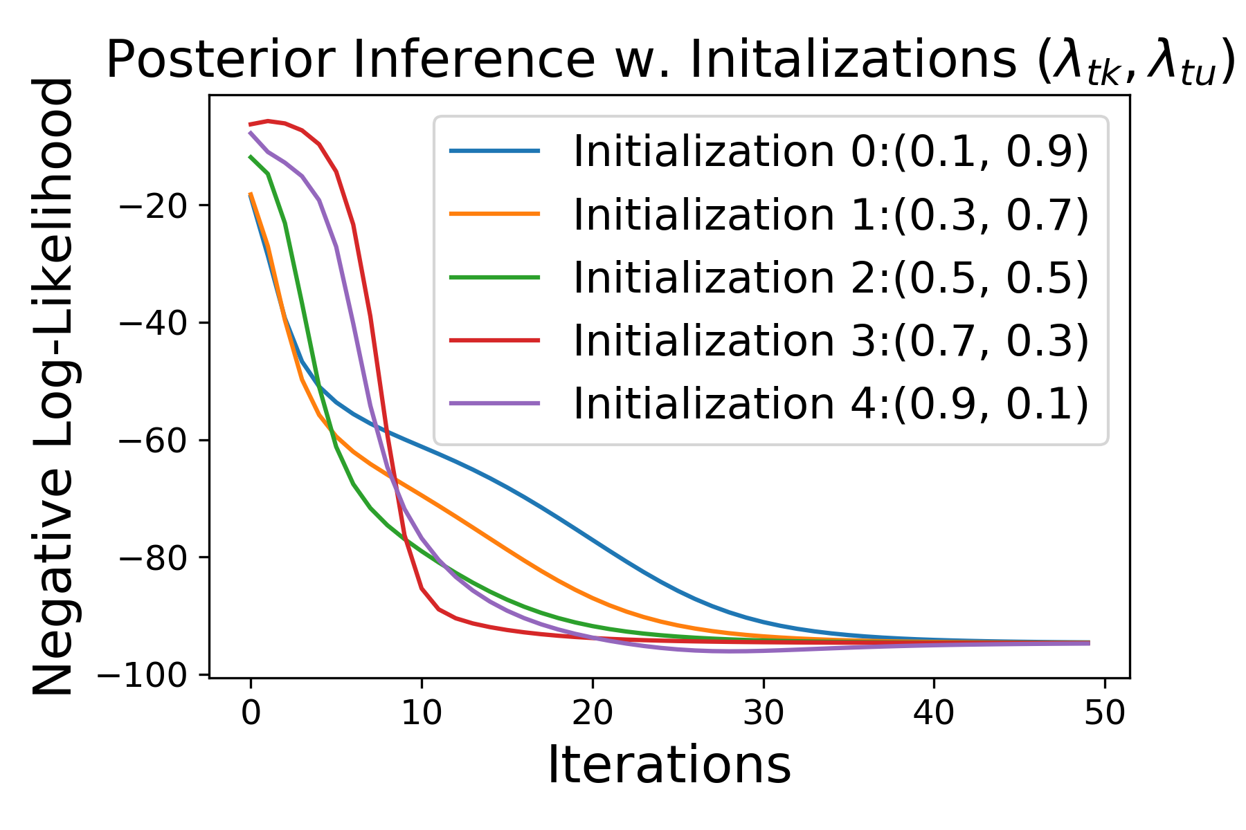
The computational complexity of UADAL is increased because we need to fit the mixture model, which requires $O(nk)$, with the number of the target instances ($n$) and the iterations of EM ($k$). Figure 11 shows the negative log-likelihood from the fitted mixture model over EM iterations ($k$), along different initializations of $\lambda_{tk}$ and $\lambda_{tu}$. Here, $k$ can be adjusted to trade the performance (negative log-likelihood) and the time-complexity ($k$). Moreover, it shows that the convergence of EM algorithm of the posterior inference, which makes we set $k$ as constant. As a measure of the computational complexity, we provide Wall-clock-time for a whole experimental procedure by following Algorithm 1 (under an RTX3090 GPU/i7-10700F CPU). For A$\rightarrow$W in Office-31, the wall-clock-time is 1,484 and 1,415 seconds, with and without posterior inference, respectively (+5% increment). From this +5% increment, the performance of UADAL with the posterior inference has improved than with Entropy, as shown in Figure 9 in the main paper (see the red/blue solid lines).

Figure 11: Convergence over EM iterations ($k$) of Posterior Inference

Appendix C Experimental Part

C.1 Implemenation details

C.1.1 Optimization Details

We utilize the pre-trained ResNet-50 [16], DenseNet-121 [17], EfficientNet-B0 [45], and VGGNet [42], as a backbone network. For all cases of the experiments for the backbone networks and the datasets, we use the SGD optimizer with the cosine annealing [28] schedule for the learning rate scheduling. For the parameters in the pre-trained network of ResNet-50, DenseNet, and EfficientNet, we set the learning rate 0.1 times smaller than the parameters from the scratch, followed by [21, 6]. For VGGNet with VisDA dataset, we followed [37]. Therefore, we did not update the parameters of VGGNet and constructed fully-connected layers with 100 hidden units after the FC8 layers. In terms of the entropy loss for the target domain, we adopt a variant of the loss, FixMatch [43], in order to utilize the confident predictions of the target instances. We run each setting three times and report the averaged accuracy with standard deviation. We conduct all experiments on an NVIDIA RTX 3090 GPU and an i7-10700F CPU.

C.1.2 Network Configurations

Except for the feature extractor network $G$, the configurations of the other networks, $E$, $C$, $D$, are based on the classification network. The feature dimensions from the ResNet-50, EfficientNet-B0, and DenseNet-121 are 2048, 1280, and 1024, respectively, which are the output dimensions of $G$ (100 for VGGNet by the construction of the fully connected layer). Given the dimension, the network $C$ utilizes one middle layer between the feature and classification layer with the dimension of 256. After the middle layer, we apply a batch normalization [18] and LeakyReLU [52] with 0.2 parameter. Then, the feature after the middle layer passes to the classification layer, in which the output dimensions are $|\mathcal{C}_{s}|+1$. The network $E$ has the classification layer without any middle layer, in which the output dimension is $|\mathcal{C}_{s}|$. The network $D$ consists of the two middle layers with applying the LeakyReLU, where the output dimension is 3.

C.1.3 Hyperparameter Settings

For all cases of the experiments, we set the batch size, $m$, to 32. For the number of epochs for main training, denoted as $n_{iter}$, we set 100 for Office-31 and OfficeHome datasets. For the VisDA dataset, we set $n_{iter}$ as 10 epochs since it is a large scale. Associated with $n_{iter}$, we set the frequency to fit the posterior inference, $\eta$, as 10 epochs for Office-31 and OfficeHome, as 1 epoch for the VisDA dataset. We set 0.001 as a default learning rate with 0.1 times smaller for the network $G$ since we bring the pre-trained network. For the network $E$ of the open-set recognizer, we set 2 times larger than the default value because the shallow network $E$ should learn the labeled source domain quickly during $\eta$ epochs, followed by initializing the network $E$ after fitting the posterior inference. For the case of VGGNet with the VisDA dataset, we utilize the default learning rate for the network $G$ as same as the other networks since we only train the fully connected layers on the top of VGGNet.

C.1.4 Baselines

For the baselines, we implement the released codes for OSBP [37] (https://github.com/ksaito-ut/OPDA_BP), STA [21] (https://github.com/thuml/Separate_to_Adapt), PGL [29] (https://github.com/BUserName/PGL), ROS [6] (https://github.com/silvia1993/ROS), DANCE [38] (https://github.com/VisionLearningGroup/DANCE), and DCC [20] (https://github.com/Solacex/Domain-Consensus-Clustering). For OSLPP [51], we are not able to find the released code. Thus, the reported performances of OSLPP for Office-31 and Office-Home with ResNet-50 are only available. For the released codes, we follow their initial experimental settings. Especially, we set all experimental settings for DenseNet and EfficientNet, equal to the settings on their ResNet-50 experiments, since they do not conduct the experiments on the DenseNet-121 and EfficientNet-B0. For a fair comparison, we bring the reported results for the baselines from its papers on the datasets, i.e., Office-31 (with ResNet-50), OfficeHome (with ResNet-50), and VisDA(with VGGNet) dataset. The officially reported performances are marked as ^∗ in the tables. Except for these cases, we all re-implement the experiments three times.

C.1.5 Dataset

For the availability of the datasets, we utilize the following links; Office-31 (https://www.cc.gatech.edu/~judy/domainadapt/#datasets_code), Office-Home (https://www.hemanthdv.org/officeHomeDataset.html), and VisDA (http://ai.bu.edu/visda-2017/#download). We utilize the data transformations for training the proposed model, which are 1) resize, random horizontal flip, crop, and normalize by following [38], and 2) RandAugment [9] by following [35].

C.2 Experimental Results

C.2.1 Computational Complexity of OSLPP on VisDA dataset

As OSLPP [51] said, their complexity is $\mathcal{O}(T(2n^{2}d_{PCA}+{d^{3}}_{PCA}))$, which is repeated for $T$ times. Here, $n$ is the number of samples with $n=n_{s}+n_{t}$, and $d_{PCA}$ is the dimension which is reduced by PCA. However, regarding memory usage, when the number of samples, $n$, is much greater than the dimensionality, the memory complexity is $\mathcal{O}(n^{2})$. Therefore, they claimed that it has limitation of scaling up to the extremely large dataset (e.g., $n>100,000$). With this point, VisDA dataset consists of the source dataset with 79,765 instances and the target dataset with 55,388 instances, where the number of samples becomes 135,153. Therefore, OSLPP is infeasible to conduct the experiments for VisDA dataset.

C.2.2 Low Accuracy of Baselines

HOS score is a harmonic mean of OS^∗ and UNK. Therefore, HOS is higher when performing well in both known and unknown classification. With this point, some baselines have very low HOS score in the Table 1 and 2 of the main paper. This is because their UNK performances are worse. For example, the reported OS and OS^∗ of PGL [29] in Office-Home are 74.0 and 76.1, respectively. Here, OS is the class-wise averaged accuracy over the classes including unknown class. With 25 known classes, UNK then becomes (25+1)$\times\text{OS}-$25$\times$OS* = 25.1, which leads to HOS score as 33.5. It means that PGL fails in the open-set scenario because their adversarial loss includes all target instances, which is critically weakened by the negative transfer.

For DANCE, they only reported OS scores in the paper, which makes the calculation of HOS infeasible. Also, their class set (15 knowns in OfficeHome) is different from the standard OSDA scenario (25 knowns in OfficeHome by following [37]). It means that optimal hyper-parameters are not available. Therefore, we re-implement based on their official code. Meanwhile, DANCE (also DCC) is based on clustering which means that they are weak on initializations or hyperparameters, empirically shown as higher standard deviations of the performances in the tables. The below is the detailed answer on the lower performances of baselines, especially DANCE, with EfficientNet. As we said, there is no reported performance of DANCE with the additional backbone choices. Therefore, we implemented additional variants of DANCE with EfficientNet and DenseNet by following their officially released codes. In order to compare fairly, we set all hyper-parameters with that of ResNet-50 case as UADAL is being set. Specifically, DANCE requires a threshold value ($\rho$) to decide whether a target instance belongs to “known” class or not, which is very sensitive to the performance. We confirmed that they utilize the different values over the experimental settings. This sensitivity may degrade the performance of DANCE. Unlike DANCE, UADAL does not require a threshold setting because it has a posterior inference to automatically find the threshold to decide open-set instances. Therefore, this becomes the key reason behind the performance difference.

For DCC, the experimental settings for VisDA are not available with the comments of “the clustering on VisDA is not very stable” in their official code repository. Threfore, our re-implementation of DCC with VisDA (with EfficientNet-B0, DenseNet-121, and ResNet50) was also unstable. For a fair comparison with DCC, please refer to the performances which is marked as ^∗ in the Table 1 and 2 of the main paper.

C.2.3 t-SNE Visualization

Figure 12 and 13 in this script represents the t-SNE visualizations of the learned features extracted by EfficientNet-B0 and ResNet-50, respectively. It should be noted that EfficientNet-B0 (5.3M) has only 20% of parameters than ResNet-50 (25.5M). We observe that the target-unknown (red) features from the baselines are not discriminated with the source (green) and the target-known (blue) features. On the contrary, UADAL and cUADAL align the features from the source and the target-known instances accurately with clear segregation of the target-unknown features. It means that UADAL learns the feature spaces effectively even in the less complexity.

(a) DANN

(b) STA

(c) OSBP

(d) DCC

(e) UADAL

(f) cUADAL

Figure 12: t-SNE of the features by the EfficientNet-B0 on the task D $\rightarrow$ W of Office-31. (blue: target-known, red: target-unkonwn, green: source)

(a) DANN

(b) STA

(c) OSBP

(d) DCC

(e) UADAL

(f) cUADAL

Figure 13: t-SNE of the features by the ResNet-50 on the task D $\rightarrow$ W of Office-31. (blue: target-known, red: target-unkonwn, green: source)

C.2.4 Proxy $\mathcal{A}$-Distance (PAD)

Proxy $\mathcal{A}$-Distance (PAD) is an empirical measure of distance between domain distributions, which is proposed by [12]. Given a generalization error $\epsilon$ of discriminating data which sampled by the domain distributions, PAD value can be computed as $\hat{d}_{\mathcal{A}}=2(1-2\epsilon)$. We compute the PAD value between target-known and target-unknown features from the feature extractor, $G$. We follow the detailed procedure in [12]. Note that high PAD value means two domain distributions are well discriminated.

C.2.5 Robust on Early Stage Iterations

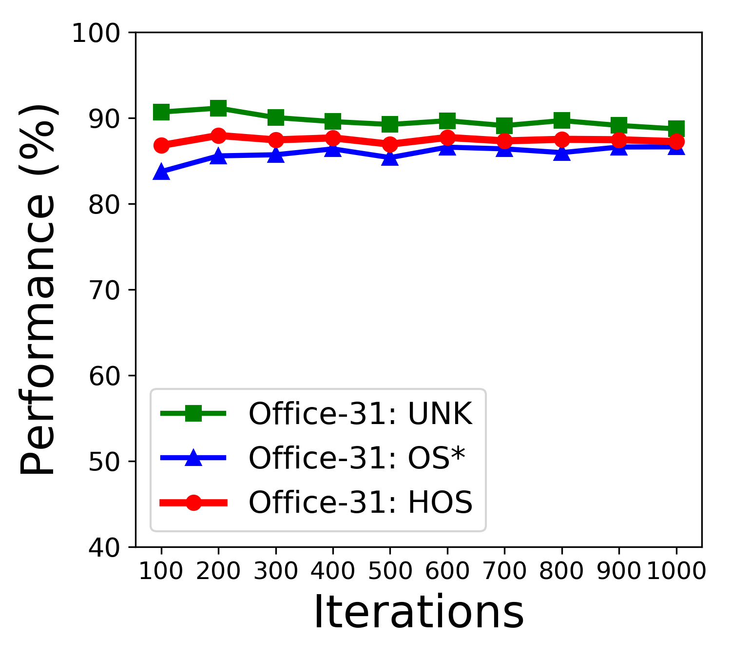
We investigate the effects of the learning iterations for the early stage training to fit the posterior inference, which is considered as a hyper-parameter of UADAL. Figure 14 represents the performance metrics such as OS^∗, UNK, and HOS over the number of the initial training iterations of UADAL. It shows that UADAL is not sensitive to the number of iterations for the early stage. Taken together with Figure 9 in the main paper, these results represent that our two modality assumption for the target entropy values robustly holds.

Figure 14: Averaged performance over the tasks in Office-31 varying the number of iterations.

C.2.6 Ablation Studies on Using Classifier $C$ as Entropy

Office31 (ResNet-50)
Network	A $\rightarrow$ W			A $\rightarrow$ D			D $\rightarrow$ W			W $\rightarrow$ D			D $\rightarrow$ A			W $\rightarrow$ A			Avg.
	OS*	UNK	HOS	OS*	UNK	HOS	OS*	UNK	HOS	OS*	UNK	HOS	OS*	UNK	HOS	OS*	UNK	HOS	OS*	UNK	HOS
C	80.5	92.4	86.1	79.4	91.0	84.8	99.0	98.3	98.6	98.7	100.0	99.3	68.7	89.7	77.9	56.5	89.1	68.9	80.5	93.4	85.9
E	84.3	94.5	89.1	85.1	87.0	86.0	99.3	96.3	97.8	99.5	99.4	99.5	73.3	87.3	79.7	67.4	88.4	76.5	84.8	92.1	88.1
Office-Home (ResNet-50)
Network	P$\rightarrow$R			P$\rightarrow$C			P$\rightarrow$A			A$\rightarrow$P			A$\rightarrow$R			A$\rightarrow$C
	OS*	UNK	HOS	OS*	UNK	HOS	OS*	UNK	HOS	OS*	UNK	HOS	OS*	UNK	HOS	OS*	UNK	HOS
C	68.8	83.7	75.5	39.3	79.4	52.6	47.9	84.3	61.1	65.0	76.3	70.2	78.4	75.6	77.0	46.7	77.2	58.2
E	71.6	83.1	76.9	43.4	81.5	56.6	50.5	83.7	63.0	69.1	72.5	70.8	81.3	73.7	77.4	54.9	74.7	63.2
Network	R$\rightarrow$A			R$\rightarrow$P			R$\rightarrow$C			C$\rightarrow$R			C$\rightarrow$A			C$\rightarrow$P			Avg.
	OS*	UNK	HOS	OS*	UNK	HOS	OS*	UNK	HOS	OS*	UNK	HOS	OS*	UNK	HOS	OS*	UNK	HOS	OS*	UNK	HOS
C	64.2	79.2	71.0	75.5	78.6	77.0	44.9	71.7	55.2	63.0	75.0	68.5	49.9	77.4	60.7	57.8	79.2	66.8	58.4	78.1	66.1
E	66.7	78.6	72.1	77.4	76.2	76.8	51.1	74.5	60.6	69.1	78.3	73.4	53.5	80.5	64.2	62.1	78.8	69.5	62.6	78.0	68.7

Table 5: Ablation study for the network $C$ and $E$ to generate the entropy value in UADAL w.r.t. classification accuracies (%) on Office-31 and Office-Home wiht ResNet-50 (bold: best performer).

This part introduces an ablation study for utilizing the classifier $C$ to generate the entropy values instead of an open-set recognizer $E$. Using the classifier $C$ (except the last unknown dimension) directly is also feasible, as $E$ does. Although it is feasible, however, it leads to wrong decisions for the target-unknown instances. As we explained, the network $E$ learns the decision boundary over $\mathcal{C}_{s}$ classes while the network $C$ does over $\mathcal{C}_{s}+1$ including unknown class. Especially, in the case of the target-unknown instances, the network $C$ is enforced to classify the instances as unknown class, which is $C_{s}+1$-th dimension. When optimizing the network $C$ with the target-unknown instances, we expect that the output of the network $C$ would have a higher value on the unknown dimension. With this point, if we use the first $C_{s}$ dimension of $C$ to calculate the entropy value, there is no evidence that the distribution of the $C$’s output is flat over $\mathcal{C}_{s}$ classes which implies to a higher entropy value. Even though the largest predicted value except the last dimension is small, the entropy value might be lower due to imbalance in the output. Then, it becomes to be considered as known class, which is wrong decision for the target-unknown instances. Therefore, it gives the negative effects on the open-set recognition, and it adversely affects when training the model.

As an ablation experiment, we conduct the experiments to compare using $E$ or $C$ for the entropy. The experimental results on both cases are shown in Table 5 of this section, applied to Office-31 and Offce-Home datasets. The network $E$ in Table 5 is the current UADAL model and $C$ represents that the entropy values are generated by the classifier $C$ without introducing the network $E$. As you can see, the performances with $E$ is better than $C$. It means that the network $E$ learns the decision boundary for the known classes, and it leads to recognize the open-set instances effectively. It should be noted that we utilize the structure of $E$ as an one-layered network to reduce the computation burden.

C.2.7 Ablation Studies on Entropy Minimization

The entropy minimization is important part for the fields such as semi-supervised learning [15, 43] and domain adaptation [25, 21, 38, 6] where the label information of the dataset is not available. In order to show the effect of this term, we conduct the ablation study on the datasets of Office-31 and Office-Home. We provide the experimental results in Table 6. Combined with the results in the main paper, the experimental result shows that UADAL without the entropy minimization loss still performs better than other baselines. It represents that UADAL learns the feature space appropriately as we intended to suit Open-Set Domain Adaptation. The properly learned feature space leads to effectively classify the target instances without the entropy minimization.

Office31 (ResNet-50)
Entropy	A $\rightarrow$ W			A $\rightarrow$ D			D $\rightarrow$ W			W $\rightarrow$ D			D $\rightarrow$ A			W $\rightarrow$ A			Avg.
Minimization	OS*	UNK	HOS	OS*	UNK	HOS	OS*	UNK	HOS	OS*	UNK	HOS	OS*	UNK	HOS	OS*	UNK	HOS	OS*	UNK	HOS
X	85.9	84.4	85.1	84.7	83.6	84.2	95.6	98.9	97.2	98.7	100.0	99.3	75.2	86.0	80.3	72.6	87.4	79.3	85.4	90.0	87.5
O	84.3	94.5	89.1	85.1	87.0	86.0	99.3	96.3	97.8	99.5	99.4	99.5	73.3	87.3	79.7	67.4	88.4	76.5	84.8	92.1	88.1
Office-Home (ResNet-50)
Entropy	P$\rightarrow$R			P$\rightarrow$C			P$\rightarrow$A			A$\rightarrow$P			A$\rightarrow$R			A$\rightarrow$C
Minimization	OS*	UNK	HOS	OS*	UNK	HOS	OS*	UNK	HOS	OS*	UNK	HOS	OS*	UNK	HOS	OS*	UNK	HOS
X	70.7	78.2	74.2	48.4	76.6	59.3	49.9	76.2	60.3	64.5	79.4	71.2	78.8	75.2	77.0	56.3	75.1	64.3
O	71.6	83.1	76.9	43.4	81.5	56.6	50.5	83.7	63.0	69.1	72.5	70.8	81.3	73.7	77.4	54.9	74.7	63.2
	R$\rightarrow$A			R$\rightarrow$P			R$\rightarrow$C			C$\rightarrow$R			C$\rightarrow$A			C$\rightarrow$P			Avg.
	OS*	UNK	HOS	OS*	UNK	HOS	OS*	UNK	HOS	OS*	UNK	HOS	OS*	UNK	HOS	OS*	UNK	HOS	OS*	UNK	HOS
X	62.3	76.4	68.6	71.3	81.0	75.8	57.3	65.6	61.2	68.1	75.9	71.8	54.7	70.9	61.7	60.1	72.6	65.8	61.9	75.2	67.6
O	66.7	78.6	72.1	77.4	76.2	76.8	51.1	74.5	60.6	69.1	78.3	73.4	53.5	80.5	64.2	62.1	78.8	69.5	62.6	78.0	68.7

Table 6: Ablation study for the entropy minimization loss in UADAL w.r.t. classification accuracies (%) on Office-31 and Office-Home wiht ResNet-50 (bold: best performer).

C.2.8 Posterior Inference with Efficiency

In terms of complexity, the posterior inference increases the computational complexity because we need to fit the mixture model. As we provided at the section B.3.2, Wall-clock-time is increased as 5% with the posterior inference in the case of full data utilization. From this +5% increment, the performance has improved significantly than that without the posterior inference (as shown in Figure 9 in the paper). In addition, by utilizing the posterior inference, we avoid introducing any extra hyper-parameter to recognize the unknown instances, which is also our contribution.

As an alternative, we fit the mixture model only by sampling the target instances in order to reduce the computation time because the computational complexity is $O(nk)$ where $n$ is the number of samples and $k$ is the number of fitting iterations (we fixed it as 10). Figure 15 represents the wall-clock time and the performance measures by sampling ratio (%) for the target domain. Since the computational complexity is linearly increased by the number of samples, the wall-clock time is also linearly increased by increasing the sampling ratio. Interestingly, we observed that even though the sampling ratio is small, i.e. 10%, the performances of UADAL w.r.t. HOS, OS*, and UNK does not decreased, on both Office-31 and Office-Home datasets.

(a) Office-31

(b) Office-Home

Figure 15: Quantitative analysis for ablation study of applying sampling on the target domain with Office-31 (a) and Office-Home (b). Each subfigure represents the Wall-Clock Time (s) increased by fitting process of the mixture model during training and HOS ($\%$) over the target sampling ratio. (All records are the averaged values over the tasks in each dataset, not just single task.)

In order to investigate the robustness on the sampling ratio, we provide the qualitative analysis in Figure 16. For each sampling ratio, the left figure represents the original target entropy distribution, and the middle shows the sampled target entropy values and the fitted BMM densities. Finally, the right figure represents the weight distribution by the posterior inference. As you can see, our posterior inference takes the entropy values, and fits the mixture model without any thresholds. Therefore, even if the sampling ratio is small, the observation that the target-unknown instances have higher entropy values than the target-known instances still holds. Therefore, the open-set recognition on the target domain is still informative, and it leads to maintain the performances of UADAL.

(a) Target Sampling Ratio: 50$\%$

(b) Target Sampling Ratio: 10$\%$

Figure 16: Qualitative analysis for ablation study of applying sampling on the target domain (D$\rightarrow$W task in Office-31). The subfigure (a) and (b) represent the different sampling ratio, 50$\%$ and 10$\%$, respectively. Each subfigure consists of 1) left: the original target entropy distribution, 2) midde: the sampled target entropy distribution with the fitted Beta Mixture Model (BMM), and 3) right: the weight ($\hat{w}$) distribution (by the fitted BMM in middle) on the target domain.

C.2.9 Full Experimental Results with All Metrics

As a reminder, HOS metric is a harmonic mean of OS* and UNK where OS* is accuracy for the known class classification and UNK is for the unknown classification. Since Open-Set Domain Adaptation should perform well on both tasks, we choose HOS metric as a primary metric. For other metrics such as OS, OS*, and UNK, we provide the full experimental results including OS, OS*, and UNK in this section. First of all, we provide the summary table of the experimental results with the officially reported performances of the baselines, which is denoted as * for reliable and fair comparisons. Table 7 in this appendix shows that UADAL outperforms the baselines over all datasets, in the conventional setting of the backbone networks (such as Office-31/Office-Home with ResNet-50 and VisDA with VGGNet). The detailed results are shown in Table 8 for Office-31 and Table 9 for Office-Home, in this appendix.

Method	Office31 (ResNet-50)				Office-Home (ResNet-50)				VisDA (VGGNet)
	OS	OS*	UNK	Avg. HOS	OS	OS*	UNK	Avg. HOS	OS	OS*	UNK	HOS
DANN	85.4	87.1	68.3	75.9$\pm$0.5	53.5	52.6	77.1	60.7$\pm$0.2	-	-	-	-
CDAN	86.1	88.3	63.9	73.4$\pm$1.3	55.3	54.5	74.6	61.4$\pm$0.3	-	-	-	-
OSBP∗	86.6	87.2	80.4	83.7$\pm$0.4	64.2	64.1	66.3	64.7$\pm$0.2	62.9	59.2	85.1	69.8
STA∗	82.5	84.3	64.8	72.5$\pm$0.8	61.9	61.8	63.3	61.1$\pm$0.3	66.8	63.9	84.2	72.7
PGL∗	81.1	82.7	64.7	72.6$\pm$1.5	74.1	76.1	25.0	35.2	80.7	82.8	68.1	74.7
ROS∗	86.5	86.6	85.8	85.9$\pm$0.2	62.0	61.6	72.4	66.2$\pm$0.3	-	-	-	-
DANCE	91.0	94.0	60.2	73.1$\pm$1.0	72.8	74.4	35.0	44.2$\pm$0.6	-	-	-	-
DCC∗	-	-	-	86.8	-	-	-	64.2	68.8	68.0	73.6	70.7
LGU∗	-	-	-	-	71.4	72.7	38.9	50.7	70.1	69.2	75.5	72.2
OSLPP∗	89.0	89.3	85.6	87.4	64.1	63.8	71.7	67.0	-	-	-	-
UADAL	85.5	84.8	92.1	88.1$\pm$0.2	63.1	62.6	78.0	68.7$\pm$0.2	67.4	63.1	93.3	75.3
cUADAL	85.6	84.8	93.0	88.5$\pm$0.3	63.1	62.5	77.6	68.5$\pm$0.1	68.3	64.3	92.6	75.9

Table 7: Summary of the OSDA experimental results. The results in Office-31 and Office-Home are the averaged accuracies over the tasks because there are the multiple domains. (bold: best performer, underline: second-best performer, ^∗: officially reported performances.)

Office31 (ResNet-50)
	A $\rightarrow$ W				A $\rightarrow$ D				D $\rightarrow$ W
Model	OS	OS*	UNK	HOS	OS	OS*	UNK	HOS	OS	OS*	UNK	HOS
DANN	84.5	87.4	55.7	68.1	87.9	90.8	59.2	71.5	97.3	99.3	77.0	86.7
CDAN	86.7	90.3	50.7	64.9	88.6	92.2	52.4	66.8	97.2	99.6	73.2	84.3
OSBP	86.1	86.8	79.2	82.7	89.1	90.5	75.5	82.4	97.6	97.7	96.7	97.2
STA	85.0	86.7	67.6	75.9	88.5	91.0	63.9	75.0	90.6	94.1	55.5	69.8
PGL	81.4	82.7	67.9	74.6	80.5	82.1	65.4	72.8	85.7	87.5	68.1	76.5
ROS	87.3	88.4	76.7	82.1	86.6	87.5	77.8	82.4	98.7	99.3	93.0	96.0
DANCE	94.3	98.7	50.7	66.9	92.8	96.5	55.9	70.7	97.0	100.0	66.8	80.0
DCC	-	-	-	87.1	-	-	-	85.5	-	-	-	91.2
LGU	-	-	-	-	-	-	-	-	-	-	-	-
OSLPP	89.4	89.5	88.4	89.0	92.4	92.6	90.4	91.5	96.1	96.9	88.0	92.3
UADAL	85.3	84.3	94.5	89.1	85.2	85.1	87.0	86.0	99.0	99.3	96.3	97.8
cUADAL	86.4	85.5	95.1	90.1	86.0	85.6	90.4	87.9	98.6	98.7	97.7	98.2
	W $\rightarrow$ D				D $\rightarrow$ A				W $\rightarrow$ A				AVG.
	OS	OS*	UNK	HOS	OS	OS*	UNK	HOS	OS	OS*	UNK	HOS	OS	OS*	UNK	HOS
DANN	97.3	100.0	70.2	82.5	73.0	72.9	74.5	73.7	72.2	72.1	73.1	72.6	85.4	87.1	68.3	75.9$\pm$0.5
CDAN	97.0	100.0	67.3	80.5	74.5	74.9	70.6	72.7	72.5	72.8	69.3	71.0	86.1	88.3	63.9	73.4$\pm$1.3
OSBP	97.7	99.1	84.2	91.1	75.8	76.1	72.3	75.1	73.1	73.0	74.4	73.7	86.6	87.2	80.4	83.7$\pm$0.4
STA	83.3	84.9	67.8	75.2	81.5	83.1	65.9	73.2	66.4	66.2	68.0	66.1	82.5	84.3	64.8	72.5$\pm$0.8
PGL	81.1	82.8	64.0	72.2	78.8	80.6	61.2	69.5	79.1	80.8	61.8	70.1	81.1	82.7	64.7	72.6$\pm$1.5
ROS	99.9	100.0	99.4	99.7	75.4	74.8	81.2	77.9	71.2	69.7	86.6	77.2	86.5	86.6	85.8	85.9$\pm$0.2
DANCE	97.6	100.0	73.7	84.8	82.4	85.3	53.6	65.8	81.6	83.7	60.6	70.2	91.0	94.0	60.2	73.1$\pm$1.0
DCC	-	-	-	87.1	-	-	-	85.5	-	-	-	84.4	-	-	-	86.8
LGU	-	-	-	-	-	-	-	-	-	-	-	-	-	-	-	-
OSLPP	95.4	95.8	91.5	93.6	81.6	82.1	76.6	79.3	78.9	78.9	78.5	78.7	89.0	89.3	85.6	87.4
UADAL	99.5	99.5	99.4	99.5	74.5	73.3	87.3	79.7	69.3	67.4	88.4	76.5	85.5	84.8	92.1	88.1$\pm$0.2
cUADAL	99.3	99.3	99.4	99.4	75.4	74.2	87.8	80.5	67.6	65.6	87.8	75.1	85.6	84.8	93.0	88.5$\pm$0.3

Table 8: Classification accuracy (%) on Office-31 dataset using ResNet-50 as the backbone network. (bold: best performer, underline: second-best performer)

Office-Home (ResNet-50)
	P$\rightarrow$R				P$\rightarrow$C				P$\rightarrow$A				A$\rightarrow$P
Model	OS	OS*	UNK	HOS	OS	OS*	UNK	HOS	OS	OS*	UNK	HOS	OS	OS*	UNK	HOS
DANN	67.9	67.7	72.0	69.8	32.3	30.1	86.3	44.6	44.0	42.4	83.9	56.3	60.4	60.0	71.3	65.2
CDAN	69.8	69.8	69.7	69.7	35.0	33.1	82.4	47.2	47.1	45.8	81.2	58.6	62.0	61.7	68.8	65.1
OSBP	76.0	76.2	71.7	73.9	45.3	44.5	66.3	53.2	59.4	59.1	68.1	63.2	71.3	71.8	59.8	65.2
STA	75.7	76.2	64.3	69.5	45.1	44.2	67.1	53.2	54.9	54.2	72.4	61.9	67.2	68.0	48.4	54.0
PGL	82.6	84.8	27.6	41.6	58.4	59.2	38.4	46.6	72.2	73.7	34.7	47.2	77.1	78.9	32.1	45.6
ROS	71.1	70.8	78.4	74.4	47.5	46.5	71.2	56.3	57.6	57.3	64.3	60.6	68.5	68.4	70.3	69.3
DANCE	84.2	86.5	27.1	41.2	48.9	48.2	67.4	55.7	69.7	70.7	43.9	54.2	82.2	84.0	35.4	49.8
DCC	-	-	-	64.0	-	-	-	52.8	-	-	-	59.5	-	-	-	67.4
LGU	81.2	82.8	41.2	55.0	53.1	54.5	18.1	27.2	68.4	69.1	50.9	58.6	79.3	80.5	49.3	61.2
OSLPP	76.8	77.0	71.2	74.0	53.6	53.1	67.1	59.3	55.4	54.6	76.2	63.6	72.5	72.5	73.1	72.8
UADAL	72.1	71.6	83.1	76.9	44.9	43.4	81.5	56.6	51.8	50.5	83.7	63.0	69.2	69.1	72.5	70.8
cUADAL	71.7	71.2	83.4	76.8	42.7	41.2	80.7	54.6	52.1	50.9	82.4	62.9	69.6	69.4	73.9	71.6
	A$\rightarrow$R				A$\rightarrow$C				R$\rightarrow$A				R$\rightarrow$P
	OS	OS*	UNK	HOS	OS	OS*	UNK	HOS	OS	OS*	UNK	HOS	OS	OS*	UNK	HOS
DANN	74.8	75.1	67.3	71.0	38.9	37.1	82.7	51.2	57.6	56.8	77.1	65.4	69.5	69.6	67.2	68.4
CDAN	74.8	75.2	66.7	70.7	41.2	39.7	78.9	52.9	60.4	59.8	73.6	66.0	70.6	70.9	64.6	67.6
OSBP	78.8	79.3	67.5	72.9	50.6	50.2	61.1	55.1	66.1	66.1	67.3	66.7	76.0	76.3	68.6	72.3
STA	77.9	78.6	60.4	68.3	47.0	46.0	72.3	55.8	67.5	67.5	66.7	67.1	76.3	77.1	55.4	64.5
PGL	85.9	87.7	40.9	55.8	61.6	63.3	19.1	29.3	78.6	81.5	6.1	11.4	83.0	84.8	38.0	52.5
ROS	75.9	75.8	77.2	76.5	51.5	50.6	74.1	60.1	67.1	67.0	70.8	68.8	72.3	72.0	80.0	75.7
DANCE	87.4	89.8	25.3	39.4	54.4	54.4	53.7	53.1	76.8	79.2	16.7	27.5	84.1	86.2	29.6	44.0
DCC	-	-	-	80.6	-	-	-	52.9	-	-	-	56.0	-	-	-	62.7
LGU	85.0	86.5	47.5	61.3	57.6	58.6	32.6	41.9	76.4	77.5	48.9	60.0	81.8	83.2	46.8	59.9
OSLPP	79.7	80.1	69.4	74.3	56.3	55.9	67.1	61.0	61.3	60.8	75.0	67.2	78.1	78.4	70.8	74.4
UADAL	81.0	81.3	73.7	77.4	55.7	54.9	74.7	63.2	67.1	66.7	78.6	72.1	77.3	77.4	76.2	76.8
cUADAL	81.8	82.2	73.3	77.5	55.8	55.0	75.6	63.6	67.3	66.8	79.6	72.6	77.7	77.8	75.6	76.7
	R$\rightarrow$C				C$\rightarrow$R				C$\rightarrow$A				C$\rightarrow$P				AVG.
	OS	OS*	UNK	HOS	OS	OS*	UNK	HOS	OS	OS*	UNK	HOS	OS	OS*	UNK	HOS	OS	OS*	UNK	HOS
DANN	38.8	37.1	80.9	50.9	61.6	61.1	73.5	66.7	45.4	43.8	84.3	57.6	51.2	50.1	77.6	60.9	53.5	52.6	77.1	60.7$\pm$0.2
CDAN	41.7	40.3	75.8	52.7	62.0	61.5	73.7	67.1	46.4	44.9	82.8	58.2	52.6	51.6	76.8	61.7	55.3	54.5	74.6	61.4$\pm$0.3
OSBP	48.6	48.0	63.0	54.5	71.9	72.0	69.2	70.6	59.8	59.4	70.3	64.3	66.8	67.0	62.7	64.7	64.2	64.1	66.3	64.7$\pm$0.2
STA	50.3	49.9	61.1	54.5	67.0	67.0	66.7	66.8	51.9	51.4	65.0	57.4	61.7	61.8	59.1	60.4	61.9	61.8	63.3	61.1$\pm$0.3
PGL	66.2	68.8	0.0	0.0	68.8	70.2	33.8	45.6	82.8	85.9	5.3	10.0	72.0	73.9	24.5	36.8	74.1	76.1	25.0	35.2
ROS	52.3	51.5	73.0	60.4	65.6	65.3	72.2	68.6	54.1	53.6	65.5	58.9	60.3	59.8	71.6	65.2	62.0	61.6	72.4	66.2$\pm$0.3
DANCE	59.4	60.1	41.3	48.3	81.3	83.9	18.4	30.2	71.2	72.9	28.4	40.9	74.6	76.3	32.8	45.9	72.8	74.4	35.0	44.2$\pm$0.6
DCC	-	-	-	76.9	-	-	-	67.0	-	-	-	49.8	-	-	-	66.6	-	-	-	64.2
LGU	62.1	63.4	29.6	40.4	76.4	77.6	46.4	58.1	65.8	67.2	30.8	42.2	69.1	71.7	4.1	7.8	71.4	72.7	38.9	50.7
OSLPP	54.8	54.4	64.3	59.0	67.5	67.2	73.9	70.4	50.7	49.6	79.0	60.9	62.1	61.6	73.3	66.9	64.1	63.8	71.7	67.0
UADAL	52.0	51.1	74.5	60.6	69.4	69.1	78.3	73.4	54.5	53.5	80.5	64.2	62.8	62.1	78.8	69.5	63.1	62.6	78.0	68.7$\pm$0.2
cUADAL	52.5	51.8	71.1	59.9	69.5	69.3	76.3	72.6	54.9	53.8	82.0	65.0	61.8	61.1	77.4	68.3	63.1	62.5	77.6	68.5$\pm$0.1

Table 9: Classification accuracy (%) on Office-Home dataset using ResNet-50 as the backbone network. (bold: best performer, underline: second-best performer)

Appendix D Limitations and Potential Negative Societal Impacts

Limitations Our domain adaptation setting assumes that we have an access to a labeled source dataset and an unlabeled target dataset, simultaneously. Thus, we may encounter the situation where the access for the source dataset and the target dataset is not available at the same time, i.e. streamlined data gathering. In addition, our work solves the Open-Set Domain Adaptation problem. It intrinsically assumes the existence of ‘unknown’ information in the target domain. Our open-set recognition is based on this assumption, thus we fit the mixture model where each mode represents for known/unknown information. We think that the common assumption of the high entropy value on target-unknowns could be considered as a limitation, as well.

Potential Negative Societal Impacts Because open-set domain adaptation focuses on categories belonging to the class of the source dataset, it is infeasible to distinguish differences between categories that are only within the target dataset. Therefore, if the source dataset’s categories are not sufficient, important categories within the target dataset may not be classified, which would lead to only limited applications when we have social stratifications.

References

- Arazo et al. [2019] E. Arazo, D. Ortego, P. Albert, N. O’Connor, and K. Mcguinness. Unsupervised label noise modeling and loss correction. In International Conference on Machine Learning, pages 312–321, 2019.
- Baktashmotlagh et al. [2014] M. Baktashmotlagh, M. T. Harandi, B. C. Lovell, and M. Salzmann. Domain adaptation on the statistical manifold. In Proceedings of the IEEE conference on computer vision and pattern recognition, pages 2481–2488, 2014.
- Ben-David et al. [2010] S. Ben-David, J. Blitzer, K. Crammer, A. Kulesza, F. Pereira, and J. W. Vaughan. A theory of learning from different domains. Machine learning, 79(1):151–175, 2010.
- Bendale and Boult [2016] A. Bendale and T. E. Boult. Towards open set deep networks. In Proceedings of the IEEE Conference on Computer Vision and Pattern Recognition (CVPR), June 2016.
- Borgwardt et al. [2006] K. M. Borgwardt, A. Gretton, M. J. Rasch, H.-P. Kriegel, B. Schölkopf, and A. J. Smola. Integrating structured biological data by kernel maximum mean discrepancy. Bioinformatics, 22(14):e49–e57, 2006.
- Bucci et al. [2020] S. Bucci, M. R. Loghmani, and T. Tommasi. On the effectiveness of image rotation for open set domain adaptation. In European Conference on Computer Vision, pages 422–438. Springer, 2020.
- Chen et al. [2020] G. Chen, L. Qiao, Y. Shi, P. Peng, J. Li, T. Huang, S. Pu, and Y. Tian. Learning open set network with discriminative reciprocal points. In European Conference on Computer Vision, pages 507–522. Springer, 2020.
- Chen et al. [2021] G. Chen, P. Peng, X. Wang, and Y. Tian. Adversarial reciprocal points learning for open set recognition. arXiv preprint arXiv:2103.00953, 2021.
- Cubuk et al. [2020] E. D. Cubuk, B. Zoph, J. Shlens, and Q. V. Le. Randaugment: Practical automated data augmentation with a reduced search space. In Proceedings of the IEEE/CVF Conference on Computer Vision and Pattern Recognition Workshops, pages 702–703, 2020.
- Fang et al. [2020] Z. Fang, J. Lu, F. Liu, J. Xuan, and G. Zhang. Open set domain adaptation: Theoretical bound and algorithm. IEEE Transactions on Neural Networks and Learning Systems, pages 1–14, 2020. doi: 10.1109/TNNLS.2020.3017213.
- Ganin and Lempitsky [2015] Y. Ganin and V. Lempitsky. Unsupervised domain adaptation by backpropagation. In International conference on machine learning, pages 1180–1189. PMLR, 2015.
- Ganin et al. [2016] Y. Ganin, E. Ustinova, H. Ajakan, P. Germain, H. Larochelle, F. Laviolette, M. Marchand, and V. Lempitsky. Domain-adversarial training of neural networks. The Journal of Machine Learning Research, 17(1):2096–2030, 2016.
- Goodfellow et al. [2014] I. Goodfellow, J. Pouget-Abadie, M. Mirza, B. Xu, D. Warde-Farley, S. Ozair, A. Courville, and Y. Bengio. Generative adversarial nets. In Advances in neural information processing systems, pages 2672–2680, 2014.
- Grandvalet and Bengio [2004] Y. Grandvalet and Y. Bengio. Semi-supervised learning by entropy minimization. Advances in neural information processing systems, 17, 2004.
- Grandvalet and Bengio [2005] Y. Grandvalet and Y. Bengio. Semi-supervised learning by entropy minimization. In Advances in neural information processing systems, pages 529–536, 2005.
- He et al. [2016] K. He, X. Zhang, S. Ren, and J. Sun. Deep residual learning for image recognition. In Proceedings of the IEEE Conference on Computer Vision and Pattern Recognition (CVPR), June 2016.
- Huang et al. [2017] G. Huang, Z. Liu, L. Van Der Maaten, and K. Q. Weinberger. Densely connected convolutional networks. In Proceedings of the IEEE conference on computer vision and pattern recognition, pages 4700–4708, 2017.
- Ioffe and Szegedy [2015] S. Ioffe and C. Szegedy. Batch normalization: Accelerating deep network training by reducing internal covariate shift. arXiv preprint arXiv:1502.03167, 2015.
- Kumar et al. [2020] A. Kumar, T. Ma, and P. Liang. Understanding self-training for gradual domain adaptation. In International Conference on Machine Learning, pages 5468–5479. PMLR, 2020.
- Li et al. [2021] G. Li, G. Kang, Y. Zhu, Y. Wei, and Y. Yang. Domain consensus clustering for universal domain adaptation. In Proceedings of the IEEE/CVF Conference on Computer Vision and Pattern Recognition, pages 9757–9766, 2021.
- Liu et al. [2019] H. Liu, Z. Cao, M. Long, J. Wang, and Q. Yang. Separate to adapt: Open set domain adaptation via progressive separation. In Proceedings of the IEEE Conference on Computer Vision and Pattern Recognition, pages 2927–2936, 2019.
- Liu et al. [2021] H. Liu, J. Wang, and M. Long. Cycle self-training for domain adaptation. Advances in Neural Information Processing Systems, 34, 2021.
- Long et al. [2015a] M. Long, Y. Cao, J. Wang, and M. I. Jordan. Learning transferable features with deep adaptation networks. In Proceedings of the 32nd International Conference on International Conference on Machine Learning-Volume 37, pages 97–105, 2015a.
- Long et al. [2015b] M. Long, Y. Cao, J. Wang, and M. I. Jordan. Learning transferable features with deep adaptation networks. In Proceedings of the 32nd International Conference on International Conference on Machine Learning - Volume 37, ICML’15, page 97–105. JMLR.org, 2015b.
- Long et al. [2016] M. Long, H. Zhu, J. Wang, and M. I. Jordan. Unsupervised domain adaptation with residual transfer networks. In Advances in neural information processing systems, pages 136–144, 2016.
- Long et al. [2017a] M. Long, Z. Cao, J. Wang, and M. I. Jordan. Conditional adversarial domain adaptation. arXiv preprint arXiv:1705.10667, 2017a.
- Long et al. [2017b] M. Long, H. Zhu, J. Wang, and M. I. Jordan. Deep transfer learning with joint adaptation networks. In International conference on machine learning, pages 2208–2217. PMLR, 2017b.
- Loshchilov and Hutter [2016] I. Loshchilov and F. Hutter. Sgdr: Stochastic gradient descent with warm restarts. arXiv preprint arXiv:1608.03983, 2016.
- Luo et al. [2020] Y. Luo, Z. Wang, Z. Huang, and M. Baktashmotlagh. Progressive graph learning for open-set domain adaptation. In International Conference on Machine Learning, pages 6468–6478. PMLR, 2020.
- Mey and Loog [2016] A. Mey and M. Loog. A soft-labeled self-training approach. In 2016 23rd International Conference on Pattern Recognition (ICPR), pages 2604–2609. IEEE, 2016.
- Neal et al. [2018] L. Neal, M. Olson, X. Fern, W.-K. Wong, and F. Li. Open set learning with counterfactual images. In Proceedings of the European Conference on Computer Vision (ECCV), pages 613–628, 2018.
- Oza and Patel [2019] P. Oza and V. M. Patel. C2ae: Class conditioned auto-encoder for open-set recognition. In Proceedings of the IEEE/CVF Conference on Computer Vision and Pattern Recognition, pages 2307–2316, 2019.
- Pan et al. [2010] S. J. Pan, I. W. Tsang, J. T. Kwok, and Q. Yang. Domain adaptation via transfer component analysis. IEEE transactions on neural networks, 22(2):199–210, 2010.
- Peng et al. [2017] X. Peng, B. Usman, N. Kaushik, J. Hoffman, D. Wang, and K. Saenko. Visda: The visual domain adaptation challenge, 2017.
- Prabhu et al. [2021] V. Prabhu, S. Khare, D. Kartik, and J. Hoffman. Sentry: Selective entropy optimization via committee consistency for unsupervised domain adaptation. In Proceedings of the IEEE/CVF International Conference on Computer Vision, pages 8558–8567, 2021.
- Saenko et al. [2010] K. Saenko, B. Kulis, M. Fritz, and T. Darrell. Adapting visual category models to new domains. In Proceedings of the 11th European Conference on Computer Vision: Part IV, ECCV’10, page 213–226, Berlin, Heidelberg, 2010. Springer-Verlag. ISBN 364215560X.
- Saito et al. [2018] K. Saito, S. Yamamoto, Y. Ushiku, and T. Harada. Open set domain adaptation by backpropagation. In Proceedings of the European Conference on Computer Vision (ECCV), pages 153–168, 2018.
- Saito et al. [2020] K. Saito, D. Kim, S. Sclaroff, and K. Saenko. Universal domain adaptation through self supervision. Advances in Neural Information Processing Systems, 33, 2020.
- Scheirer et al. [2012] W. J. Scheirer, A. de Rezende Rocha, A. Sapkota, and T. E. Boult. Toward open set recognition. IEEE transactions on pattern analysis and machine intelligence, 35(7):1757–1772, 2012.
- Shu et al. [2020] Y. Shu, Y. Shi, Y. Wang, T. Huang, and Y. Tian. p-odn: prototype-based open deep network for open set recognition. Scientific reports, 10(1):1–13, 2020.
- Simonyan and Zisserman [2014] K. Simonyan and A. Zisserman. Very deep convolutional networks for large-scale image recognition. arXiv preprint arXiv:1409.1556, 2014.
- Simonyan and Zisserman [2015] K. Simonyan and A. Zisserman. Very deep convolutional networks for large-scale image recognition. In International Conference on Learning Representations, 2015.
- Sohn et al. [2020] K. Sohn, D. Berthelot, N. Carlini, Z. Zhang, H. Zhang, C. A. Raffel, E. D. Cubuk, A. Kurakin, and C.-L. Li. Fixmatch: Simplifying semi-supervised learning with consistency and confidence. Advances in Neural Information Processing Systems, 33:596–608, 2020.
- Sun et al. [2020] X. Sun, Z. Yang, C. Zhang, K.-V. Ling, and G. Peng. Conditional gaussian distribution learning for open set recognition. In Proceedings of the IEEE/CVF Conference on Computer Vision and Pattern Recognition, pages 13480–13489, 2020.
- Tan and Le [2019] M. Tan and Q. Le. Efficientnet: Rethinking model scaling for convolutional neural networks. In International Conference on Machine Learning, pages 6105–6114. PMLR, 2019.
- Tzeng et al. [2014] E. Tzeng, J. Hoffman, N. Zhang, K. Saenko, and T. Darrell. Deep domain confusion: Maximizing for domain invariance. arXiv preprint arXiv:1412.3474, 2014.
- Tzeng et al. [2017] E. Tzeng, J. Hoffman, K. Saenko, and T. Darrell. Adversarial discriminative domain adaptation. In Proceedings of the IEEE conference on computer vision and pattern recognition, pages 7167–7176, 2017.
- Van der Maaten and Hinton [2008] L. Van der Maaten and G. Hinton. Visualizing data using t-sne. Journal of machine learning research, 9(11), 2008.
- Vaze et al. [2021] S. Vaze, K. Han, A. Vedaldi, and A. Zisserman. Open-set recognition: A good closed-set classifier is all you need. arXiv preprint arXiv:2110.06207, 2021.
- Venkateswara et al. [2017] H. Venkateswara, J. Eusebio, S. Chakraborty, and S. Panchanathan. Deep hashing network for unsupervised domain adaptation. In Proceedings of the IEEE Conference on Computer Vision and Pattern Recognition (CVPR), July 2017.
- Wang et al. [2021] Q. Wang, F. Meng, and T. P. Breckon. Progressively select and reject pseudo-labelled samples for open-set domain adaptation. arXiv preprint arXiv:2110.12635, 2021.
- Xu et al. [2015] B. Xu, N. Wang, T. Chen, and M. Li. Empirical evaluation of rectified activations in convolutional network. arXiv preprint arXiv:1505.00853, 2015.
- Xu et al. [2019] R. Xu, G. Li, J. Yang, and L. Lin. Larger norm more transferable: An adaptive feature norm approach for unsupervised domain adaptation. In Proceedings of the IEEE/CVF International Conference on Computer Vision, pages 1426–1435, 2019.
- Yamano [2019] T. Yamano. Some bounds for skewed -jensen-shannon divergence. Results in Applied Mathematics, 3:100064, 2019.