Automatic Clipping: Differentially Private Deep Learning Made Easier and Stronger

Abstract

Per-example gradient clipping is a key algorithmic step that enables practical differential private (DP) training for deep learning models. The choice of clipping threshold $R$, however, is vital for achieving high accuracy under DP. We propose an easy-to-use replacement, called automatic clipping, that eliminates the need to tune $R$ for any DP optimizers, including DP-SGD, DP-Adam, DP-LAMB and many others. The automatic variants are as private and computationally efficient as existing DP optimizers, but require no DP-specific hyperparameters and thus make DP training as amenable as the standard non-private training. We give a rigorous convergence analysis of automatic DP-SGD in the non-convex setting, showing that it can enjoy an asymptotic convergence rate that matches the standard SGD, under a symmetric gradient noise assumption of the per-sample gradients (commonly used in the non-DP literature). We demonstrate on various language and vision tasks that automatic clipping outperforms or matches the state-of-the-art, and can be easily employed with minimal changes to existing codebases.

1 Introduction

Deep learning has achieved impressive progress in a wide range of tasks. These successes are made available, in part, by the collection of large datasets, sometimes containing sensitive private information of individual data points. Prior works have illustrated that deep learning models pose severe privacy risks to individual subjects in the training data and are susceptible to various practical attacks. For example, machine learning services such as Google Prediction API and Amazon Machine Learning can leak membership information from the purchase records [65]; the GPT2 language models auto-complete texts that contain someone’s full name, phone number, email address, etc., from the training data that it memorizes, if invoked by specific prefixes [11].

Differential privacy (DP) [24, 26, 25] is a formal definition of privacy that has been shown to prevent the aforementioned privacy risks in deep learning [1]. At a high level, the key difference between the DP deep learning and the standard one is whether the gradient is privately released. In other words, while the standard optimizers update on $\sum_{i}\bm{g}_{i}$, the DP optimizers update on the private gradient:

$$\text{DP Optimizer}(\{\bm{g}_{i}\}_{i=1}^{B}) =\text{Optimizer}(\overbrace{\sum\nolimits_{i}\bm{g}_{i}\cdot\texttt{Clip}(\|\bm{g}_{i}\|;R)+\sigma R\cdot\mathcal{N}(0,\mathbf{I})}^{\text{private gradient}})$$ (1.1)

$$\text{Standard Optimizer}(\{\bm{g}_{i}\}_{i=1}^{B}) =\text{Optimizer}(\sum\nolimits_{i}\bm{g}_{i})$$ (1.2)

Here $\bm{g}_{i}\in\mathbb{R}^{d}$ is the per-sample gradient of loss $l_{i}$, $\mathcal{N}$ is the standard normal, $\sigma$ is the noise multiplier, and $R$ is the clipping threshold. The clipping function $\texttt{Clip}:\mathbb{R}^{d}\to\mathbb{R}$ is defined such that $\|\bm{g}_{i}\cdot\texttt{Clip}(\bm{g}_{i};R)\|\leq R$. For instance, the DP-SGD in [1] is

$$\text{DP-SGD}_{\text{Abadi}}:\quad\bm{w}_{t+1}=\bm{w}_{t}-\eta\Big{(}\sum\nolimits_{i}\frac{\partial l_{i}}{\partial\bm{w}_{t}}\min\Big{(}R/\Big{\|}\frac{\partial l_{i}}{\partial\bm{w}_{t}}\Big{\|},1\Big{)}+\sigma R\cdot\mathcal{N}(0,\mathbf{I})\Big{)}$$ (1.3)

In comparison to the regular training (1.2), two additional DP-specific hyperparameters $R$ and $\sigma$ need to be determined in DP learning (1.1). On the one hand, setting the noise multiplier $\sigma$ is easy and can be derived analytically prior to the training. Whenever the privacy budget $(\epsilon,\delta)$ is determined, one can apply off-the-shelf privacy accounting tools in Section 2.1 to determine $\sigma$, based on the subsampling probability $p$ and the number of iterations $T$:

$$\text{privacy\_accountant}(\sigma,p,T;\delta)=\epsilon$$

On the other hand, the choice of clipping threshold $R$ is crucial to the performance of DP models, yet the hyperparameter tuning is much labor-intensive. Recent advances of DP deep learning on ImageNet [38] and on E2E datasets [41], using ResNet18 and GPT2 respectively, illustrate that the performance is very sensitive to $R$. We have reproduced their results in Figure 1. Observe that on ImageNet, ResNet18 can drop from the highest 45% accuracy to 31% if $R$ is chosen 2 times larger, and to 0.1% if $R$ is chosen 4 times larger. Similar drastic drop can also be observed in [38, Figure 3] even if the noise multiplier $\sigma=0$. Unlike the noise multiplier $\sigma$, the clipping threshold $R$ cannot be inferred from the privacy budget $(\epsilon,\delta)$ and have to be tuned. Consequently, DP training necessarily requires an expensive 2D grid search for $(R,\eta)$, like Figure 1, whereas the regular training only requires an easy 1D grid search for $\eta$. Even worse, the difficulty of tuning a per-layer clipping threshold vector [49], i.e. one clipping threshold for one layer, may increase exponentially as the number of layers increases.

To save the effort of tuning $R$, previous researches have proposed different approaches. In [3, 58, 28, 31], researchers advocate to use data-adaptive information to select $R$, such as a specified quantile of the gradient norm distribution. These adaptive clipping methods can be a little ad-hoc: they often replace the need to tune $R$ by the need to tune one or more new hyperparameters, e.g. the quantile to use and the ratio to split the privacy budget between the quantile decision and the gradient perturbation. Another approach used by the practitioners is to replace the single 2D grid search by multiple cheaper 1D grid searches. For example, the researchers propose, in [38, Section 3.3] to fine-tune $\eta$ with non-DP SGD, fix $\eta$ and sweep over various values of the clipping threshold $R$ with DP-SGD, then further fix $R$ and do one more grid search on $\eta$. However, tuning $R$ formally in a data-dependent way (e.g. through cross-validation) introduces additional privacy loss [55], and most existing empirical work does not privately conduct hyperparameter tuning.

We take a completely different route by proposing a new clipping principle that removes $R$, instead of coming up with methods to find the appropriate $R$. We term our method as automatic clipping and the DP optimizers using it as automatic DP optimizers. Our contributions are:

1. We propose the automatic clipping in (4.1) that expunges the clipping threshold from general DP optimizers, making DP training as amenable as regular training. In large-scale tasks (GPT-level) like Figure 1, our automatic clipping can reduce the cost of ablation study by $5\times$.

2. We show that automatic DP optimizers are as private and efficient as existing DP optimizers.

3. We show in Theorem 4 that automatic DP-SGD converges in the non-convex setting, at the same asymptotic convergence rate as the standard SGD. Our theoretical analysis successfully explains the training behaviors of deep learning in previous empirical works.

4. We demonstrate the superiority of automatic clipping on a variety of vision and language tasks, especially with large models including ResNet, RoBERTa and GPT2.

5. In Appendix K, we include simple code snippets that demonstrate how easy it is to switch from Abadi’s clipping to our automatic clipping in popular codebases, e.g. Opacus and ObJAX.

2 Preliminaries

2.1 Differential Privacy

We consider the $(\epsilon,\delta)$-DP in Definition 2.1, where smaller $(\epsilon,\delta)$ means stronger privacy guarantee.

Definition 2.1 ([25]).

A randomized algorithm $M$ is $(\varepsilon,\delta)$-differentially private (DP) if for any two neighboring datasets $S,S^{\prime}$ (i.e. if one can obtain $S^{\prime}$ by adding or removing one data point from $S$), and for any event $E$,

$$\mathbb{P}[M(S)\in E]\leqslant\mathrm{e}^{\varepsilon}\mathbb{P}\left[M\left(S^{\prime}\right)\in E\right]+\delta.$$ (2.1)

In words, DP restricts the influence of an arbitrary sample, so that the information contributed by such sample is limited and less vulnerable to privacy attacks. In deep learning, DP is achieved by applying the subsampled Gaussian mechanism to privatize the minibatch gradients during training.

As illustrated in Equation 1.1, the subsampled Gaussian mechanism involves (I) sampling a minibatch by including each data point iid with probability $p$ (II) per-sample gradient clipping to bound the $l_{2}$ norm sensitivity at $R$ and (III) adding independent Gaussian noise proportional to $R$ and $\sigma$, where $\sigma$ is derived from the privacy budget $(\epsilon,\delta)$. This can be realized by leveraging a variety of modern privacy accounting tools, such as Renyi DP (or moments accountant) [1, 51, 71], Privacy Loss distribution (Fourier accountants) [37, 30, 82], or Gaussian DP [19, 7].

2.2 Differentially Private optimizers with general clipping operations

Privately released stochastic gradients (through the Gaussian mechanism) can be used by various off-the-shelf optimizers, including DP-SGD in (1.3), DP-HeavyBall, DP-AdaGrad, DP-Adam, DP-FedAvg/FedSGD [49], etc. To improve the performance of DP optimizers, previous researches on the per-sample clipping can be classified into two categories.

The first category, where the majority of researches lie in, works with Abadi’s clipping and focuses on better design of $R$. To name a few examples, one can adaptively design $R_{t}$ for each iteration $t$ [3, 58, 28], or design the per-layer clipping threshold vector $\bm{R}\in\mathbb{R}^{L}$ for $L$ layers [1, 49] so as to apply a different clipping threshold for each layer.

Fewer works fall into the second category that proposes new clipping methods. In fact, any function $\texttt{Clip}:\mathbb{R}^{d}\to\mathbb{R}$ satisfying $\|\texttt{Clip}(\bm{g})\cdot\bm{g}\|\leq R$ can serve as a valid clipping function besides Abadi’s. For example, the global clipping [9] proposes $\texttt{Clip}_{\text{global}}(\bm{g}_{i}):=\mathbb{I}(\|\bm{g}_{i}\|<R)$ to mitigate the bias of the private gradient and alleviate the mis-calibration issue of DP classifiers. Another example is the re-parameterized clipping [17], $\texttt{Clip}_{\text{re-param}}(\bm{g}_{i}):=\min(1/\|\bm{g}_{i}\|,1/R)$, which is equivalent to Abadi’s clipping under a re-scaled learning rate. Our automatic clipping belongs to this category. We note that different clipping methods work orthogonally to optimizers, network architectures and gradient norm computation (see Section 8).

3 Motivation

3.1 Small clipping threshold often works best

Figure 1: Ablation study of clipping threshold and learning rate. Left: BLEU score of GPT2 on E2E dataset [41], with DP-AdamW. Right: Test accuracy of ResNet18 on ImageNet [38], with DP-SGD.

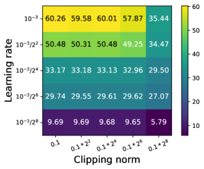
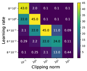
One intriguing observation that we can make about the recent studies on DP learning with large models is that the state-of-the-art (SOTA) results are often achieved with very small clipping threshold $R$. This observation is consistent in both vision and language tasks. In [41], GPT2 (about 800 million parameters) and RoBERTa models (over 300 millions parameters) achieve the best results under DP on QNLI, MNLI, SST-2, QQP, E2E, and DART datasets, with each per-sample gradient clipped to length $R=0.1$. In [38, 17, 50], ResNets and Vision Transformers achieve the best DP results on ImageNet with $R=1$; in [68], the best DP results on CIFAR10 use $R=0.1$ with ResNeXt-29 and SimCLRv2 [13]. The effectiveness of small clipping threshold together with proper learning rate is depicted in Figure 1.

Intuitively, smaller $R$ implies that the Abadi’s clipping (3.1) is effective, which means $\min\big{(}R/\|\bm{g}_{i}\|,1\big{)}=R/\|\bm{g}_{i}\|$. Given that the clipping threshold $R$ is so small compared to the number of parameters in large models, and that strong DP is guaranteed when the number of training iterations is small (i.e. $\|\bm{g}_{i}\|$ has not converged to small values yet), we expect and empirically observe that the clipping happens on a large proportion of per-sample gradients at all iterations. For instance, we find in the GPT2 generation experiments in [41] that 100% of per-sample gradients are clipped at all iterations; in classification tasks such as QQP, QNLI, and MNLI, the percentage of clipping is about $20\sim 60\%$ on average (more details in Section H.1).

3.2 Per-sample gradient normalization as new clipping

In the small clipping threshold regime, we can approximately view

$$\texttt{Clip}_{\text{Abadi}}(\bm{g}_{i};R)=\min\left(R/||\bm{g}_{i}||,1\right)\approx R/||\bm{g}_{i}||=:\texttt{Clip}_{\text{AUTO-V}}(\bm{g}_{i};R)$$ (3.1)

and thus derive a novel private gradient $\sum_{i}R\frac{\bm{g}_{i}}{\|\bm{g}_{i}\|}+\sigma R\cdot\mathcal{N}(0,\mathbf{I})$. Here AUTO-V stands for the vanilla automatic clipping, which essentially performs the normalization on each per-sample gradient. As a specific example, we can write the $R$-dependent automatic DP-SGD as

$$R\text{-dependent }\text{DP-SGD}_{\text{AUTO-V}}:\bm{w}_{t+1}=\bm{w}_{t}-\eta\Big{(}\sum_{i}R\frac{\partial l_{i}}{\partial\bm{w}_{t}}/\|\frac{\partial l_{i}}{\partial\bm{w}_{t}}\|+\sigma R\cdot\mathcal{N}(0,\mathbf{I})\Big{)}$$ (3.2)

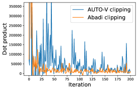
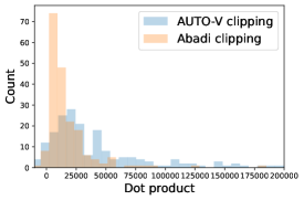
We may view our AUTO-V clipping as to maximize the dot-product similarity (a commonly used similarity measure, e.g. in the attention block in transformers [69]) between the clipped gradient and the regular gradient. Suppose we want to

$$\max_{C_{i}}\left\langle{\textstyle\sum}_{i}C_{i}\bm{g}_{i},{\textstyle\sum}_{j}\bm{g}_{j}\right\rangle\quad\text{ s.t. }0\leq C_{i}\leq R/\|\bm{g}_{i}\|$$ (3.3)

Note that the constraint is a sufficient condition for clipping, as discussed in Section 2.2. It is not hard to see that the optimal clipping factor (though violating DP guarantee) regarding (3.3) is

$$C_{i}=R/\|\bm{g}_{i}\|\cdot\mathbb{I}(\langle\bm{g}_{i},\sum\nolimits_{j}\bm{g}_{j}\rangle>0),$$ (3.4)

If the per-sample gradients are indeed concentrated in the sense $\forall i,\langle\bm{g}_{i},\sum_{j}\bm{g}_{j}\rangle\geq 0$, then AUTO-V is the optimal per-sample gradient clipping. We compare with Abadi’s clipping in Figure 2, where this similarity is significantly magnified by our AUTO-V clipping. In fact, the dot-product similarity in (3.3) closely resembles the convergence of DP optimization for Theorem 4 in (C.2).

Figure 2: RoBERTa-base with DP-Adam ($\epsilon=3$) on SST2 dataset, as in Section 6.2.

3.3 Stability constant breaks scale-invariance and remains stationary

Figure 3: Gradient (scalar) at each $\theta$.

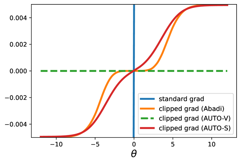
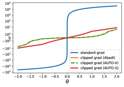
One potential drawback of AUTO-V clipping is that all gradients lose their magnitudes information completely, since $\|\bm{g}_{i}\cdot\texttt{Clip}_{\text{AUTO-V}}(\bm{g}_{i};R)\|=R,\forall i$. This scale-invariance in AUTO-V and partially in Abadi’s clipping (when $\|\bm{g}_{i}\|>R$) leads to the "lazy region" issue: the parameters will not be updated by DP-GD even if the true gradients are non-zero. In Figure 3, we illustrate such issue in a logistic regression for AUTO-V and Abadi’s clipping, when the trainable parameter $\theta\in[-2,2]$, as the gradients from two classes cancel each other.

To preserve the magnitude information and thus escape the lazy region, we propose the AUTO-S clipping, with a positive stability constant $\gamma$:

$$\texttt{Clip}_{\text{AUTO-S}}(\bm{g}_{i};R):=R/(||\bm{g}_{i}||+\gamma)$$ (3.5)

We visualize in Figure 5 that AUTO-S allows larger per-sample gradients to have larger magnitudes after the clipping, while still allowing smaller gradients to vanish after “clipping”. That is, as $\bm{g}_{i}\to 0$, the existence of $\gamma$ allows the clipped gradient $C_{i}\bm{g}_{i}\to\bm{g}_{i}/\gamma$ rather than having a magnitude $R$ as in AUTO-V. We elaborate this point in Section 4.3. This is critical in our convergence analysis and allows DP-SGD${}_{\text{AUTO-S}}$ (but not DP-SGD${}_{\text{AUTO-V}}$) to converge to zero gradient norms in Section 5.

4 Automatic DP Training

One may wonder why our clipping (3.1)(3.5) is automatic at all, if the hyperparameter $R$ is still present and there is an additional parameter $\gamma$ to choose. It turns out that any constant choice of $R>0$ is equivalent to choosing $R=1$, and common deep learning optimizers are insensitive to the choice of $\gamma$ (e.g. for any $\gamma>0$, we show that the gradient norm converges to zero at the same asymptotic rate in Theorem 4; see also the ablation study in Figure 15). Consequently, we set $\gamma=0.01$ as the default. Specifically, let us redefine the $R$-independent clipping function:

$$\texttt{Clip}_{\text{AUTO-S}}(\bm{g}_{i}):=1/(||\bm{g}_{i}||+\gamma).$$ (4.1)

With this clipping, we can design automatic DP optimizers similar to (1.1):

$$\text{Automatic DP Optimizer}(\{\bm{g}_{i}\}_{i=1}^{B}) =\text{Optimizer}\underbrace{\big{(}\sum_{i}\frac{\bm{g}_{t,i}}{||\bm{g}_{t,i}||+\gamma}+\sigma\cdot\mathcal{N}(0,\mathbf{I})\big{)}}_{\text{denoted as }\hat{\bm{g}}_{t}}$$ (4.2)

Clearly, the new private gradient $\hat{\bm{g}}_{t}$ from our automatic clipping is $R$-independent, in contrast to the one used in (1.1). A concrete example (in the case of $\gamma=0$) that is comparable to (3.2) will be

$$R\text{-independent }\text{DP-SGD}_{\text{AUTO-V}}:\quad\bm{w}_{t+1}=\bm{w}_{t}-\eta\Big{(}\sum_{i}\frac{\partial l_{i}}{\partial\bm{w}_{t}}/\Big{\|}\frac{\partial l_{i}}{\partial\bm{w}_{t}}\Big{\|}+\sigma\cdot\mathcal{N}(0,\mathbf{I})\Big{)}$$ (4.3)

Leveraging the private gradient $\hat{\bm{g}}_{t}$ in (4.2), we can train DP neural networks without tuning DP-specific hyperparamters $R$ and $\sigma$, as demonstrated in Algorithm 1.

Algorithm 1 Automatic Deep Learning with DP

Parameters: initial weights $\bm{w}_{0}$, learning rate $\eta_{t}$, sampling probability $p$, number of iterations $T$.

1:Compute $\sigma$ such that $\epsilon_{\text{Accountant}}(\delta,\sigma,p,T)\leq\epsilon$ from any privacy accountant.

2:for iteration $t=1,\cdots,T$ do

3:     Sample a batch $B_{t}$ by including each data point i.i.d. with probability $p$

4:     Apply automatic clipping to per-sample gradients $\{\bm{g}_{i}\}_{i\in B_{t}}$: $\hat{\bm{g}}_{i}=\bm{g}_{i}/(\|\bm{g}_{i}\|_{2}+0.01)$.

5:     Add Gaussian noise to the sum of clipped gradients: $\hat{\bm{g}}=\sum_{i}\hat{\bm{g}}_{i}+\sigma\cdot\mathcal{N}(0,\mathbf{I})$.

6:     Update $\bm{w}_{t}$ by any optimizer on the private gradient $\hat{\bm{g}}$ with learning rate $\eta_{t}$.

We will elaborate two distinct reasons in the next sub-sections for the following statement:

$$\boxed{\text{DP Optimizer}_{\text{Abadi}}\approx R\text{-dependent DP Optimizer}_{\text{AUTO}}\equiv R\text{-independent DP Optimizer}_{\text{AUTO}}}$$

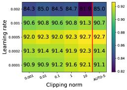
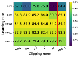
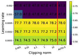
which expunges the DP hyperparameters, only leaving us the regular hyperparameters such as learning rate, weight decay, etc. The significant save in the tuning effort is illustrated in Figure 4.

Figure 4: Test accuracy of RoBERTa-base by different clipping thresholds $R$ and learning rates $\eta$. This is trained with DP-Adam (Abadi and AUTO-S) on SST2 (left, 3 epochs), QNLI (middle, 1 epoch), and MNLI (right, 1 epoch), under $\epsilon=3$. Notice by only searching along $\eta$, instead of over $(R,\eta)$, we can save the cost of hyperparameter tuning by $5\times$.

4.1 Non-adaptive optimizer couples clipping threshold with learning rate

With $R$-dependent automatic clipping, DP-SGD becomes

$$\bm{w}_{t+1}=\bm{w}_{t}-\eta\Big{(}\sum_{i}\bm{g}_{t,i}\cdot\frac{R}{||\bm{g}_{t,i}||+\gamma}+\sigma R\cdot\mathcal{N}(0,\mathbf{I})\Big{)}=\bm{w}_{t}-\eta R\hat{\bm{g}}_{t}.$$

We can view $\eta_{\text{effective}}\equiv\eta R$ as a whole: increasing $R$ has the same effect as increasing $\eta$, which explains the diagonal pattern in Figure 1(lower plot) where $\text{DP-SGD}_{\text{Abadi}}$ is applied with small clipping threshold. We extend to general non-adaptive optimizers in Theorem 1.

Theorem 1.

Non-adaptive $R$-dependent automatic DP optimizers (including SGD, Heavyball[59] and NAG[54]), with learning rate $\eta$ and weight decay $\lambda$, is equivalent to $R$-independent automatic DP optimizers, with learning rate $\eta R$ and weight decay $\lambda/R$.

4.2 Adaptive optimizer can be insensitive to clipping threshold

Adaptive automatic DP optimizers are different than the non-adaptive ones, as the clipping threshold cancels out instead of being coupled with learning rate. To see this, we scrutinize $\text{DP-Adam}_{\text{Abadi}}$ (which is similar to $\text{DP-Adam}_{\text{AUTO-V}}$) in Figure 1(upper plot), where columns to the left are almost identical. Further evidence is observed in [50, Table 5] that shrinking $R$ has zero effect on LAMB. We now give a simple explanation using AdaGrad [22]:

$$\bm{w}_{t+1}=\bm{w}_{t}-\eta\frac{\bm{g}_{t}}{\sqrt{\sum_{\tau<t}\bm{g}_{\tau}^{2}}}$$

where $\bm{g}_{t}=\sum_{i}\bm{g}_{t,i}$ is the gradient sum. In $R$-dependent DP-AdaGrad${}_{\text{AUTO-V}}$, the private gradient is $R\hat{\bm{g}}_{t}$ in place of the standard gradient sum $\bm{g}_{t}$:

$$\bm{w}_{t+1}=\bm{w}_{t}-\eta\frac{R\hat{\bm{g}}_{t}}{\sqrt{R^{2}\sum_{\tau\leq t}\hat{\bm{g}}_{\tau}^{2}}}=\bm{w}_{t}-\eta\frac{\hat{\bm{g}}_{t}}{\sqrt{\sum_{\tau<t}\left(\hat{\bm{g}}_{\tau}\right)^{2}}}.$$

We generalize to other adaptive optimizers in Theorem 2 and to the per-layer clipping style in Section B.3.

Theorem 2.

Adaptive $R$-dependent automatic DP optimizers (e.g. AdaGrad[22], AdaDelta[79], AdaMax/Adam[35], NAdam[20], RAdam[43], LARS[75], LAMB[76]), with learning rate $\eta$ and weight decay $\lambda$ is equivalent to $R$-independent automatic DP optimizers with learning rate $\eta$ and weight decay $\lambda/R$. With decoupled weight decay[46], $R$-dependent automatic DP-AdamW is equivalent to $R$-independent automatic DP-AdamW with the same $\eta$ and $\lambda$.

4.3 Automatic clipping is equally private and maximizes utility

Figure 5: Per-sample gradient norms before and after different clippings at $R=1$.

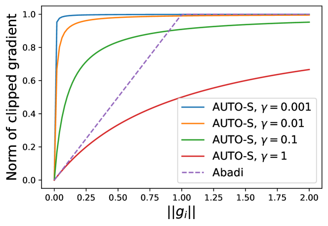
In Theorem 3 (proved in Appendix A), we show that the new private gradient $\hat{\bm{g}}_{t}$ in (4.2) has the same level of privacy guarantee as the existing one in (1.1), since the global sensitivity remains the same (see Figure 5). We note that as long as $\gamma>0$, the magnitude information of per-sample gradients is preserved by AUTO-S, in the sense that $\|\bm{g}_{i}\|>\|\bm{g}_{j}\|\Longleftrightarrow\|C_{i}\bm{g}_{i}\|>\|C_{j}\bm{g}_{j}\|$, whereas this can be violated in both the AUTO-V and Abadi’s clipping (as depicted by the flat curve in Figure 5 when $\|\bm{g}_{i}\|>1$).

Additionally, note that when $\gamma$ is small, almost all data points “max out” the signal relative to the amount of noise we add. To say it differently, for the same amount of noise, AUTO-S with small $\gamma$ allows more signal to be pushed through a differentially private channel. Towards the end of the training, i.e., at the limit when $\|\bm{g}_{i}\|\rightarrow 0$ for all $i$, then we have $\sum_{i}\frac{\bm{g}_{i}}{\|\bm{g}_{i}\|+\gamma}\rightarrow\frac{1}{\gamma}\sum_{i}\bm{g}_{i}$. In words, the clipped gradients become closer to the standard SGD, thus do not suffer from the instability of AUTO-V.

Theorem 3.

Under the noise multiplier $\sigma$, number of iterations $T$, subsampling probability $B/n$, DP optimizers using AUTO-V or AUTO-S clipping satisfy $(\epsilon_{\text{Accountant}}(\delta,\sigma,B/n,T),\delta)$-DP, where $\epsilon_{\text{Accountant}}$ is any valid privacy accountant for DP-SGD under Abadi’s clipping.

5 Convergence analysis of DP-SGD with automatic clipping

5.1 Convergence theory of DP-SGD to stationary points

We highlight that automatic clipping can be more amenable to analysis than Abadi’s clipping in [14], since we no longer need to decide whether each per-sample gradient is clipped.

To analyze the convergence of automatic DP-SGD (4.2) in the non-convex setting, we follow the standard assumptions in the SGD literature [27, 2, 6], including a symmetry assumption on the gradient noise, which is empirically verified in [14, Figure 3] and commonly used in the standard non-DP literature [48, 66, 12, 73]. We refer the curious readers to Section E.5 for details.

Assumption 5.1 (Lower bound of loss).

For all $\bm{w}$ and some constant $\mathcal{L}_{*}$, we have $\mathcal{L}(\bm{w})\geq\mathcal{L}_{*}$.

Assumption 5.2 (Smoothness).

Let $\bm{g}(\bm{w})$ denote the gradient of the objective $\mathcal{L}(\bm{w})$. Then $\forall\bm{w},\bm{v}$, there is an non-negative constant $L$ such that

$$\mathcal{L}(\bm{v})-\left[\mathcal{L}(\bm{w})+\bm{g}(\bm{w})^{\top}(\bm{v}-\bm{w})\right]\leq\frac{L}{2}\|\bm{w}-\bm{v}\|^{2}.$$ (5.1)

Assumption 5.3 (Gradient noise).

The per-sample gradient noise $\tilde{\bm{g}}_{t,i}-\bm{g}_{t}$ is i.i.d. from some ditribution such that

$$\mathbb{E}(\tilde{\bm{g}}_{t,i}-\bm{g}_{t})=0,\mathbb{E}\|\tilde{\bm{g}}_{t,i}-\bm{g}_{t}\|^{2}\leq\xi^{2},$$

and $\tilde{\bm{g}}_{t,i}$ is centrally symmetric about $\bm{g}_{t}$ in distribution: $\tilde{\bm{g}}_{t,i}-\bm{g}_{t}\overset{\mathcal{D}}{=}\bm{g}_{t}-\tilde{\bm{g}}_{t,i}.$

We show in Theorem 4 that DP-SGD with AUTO-S clipping allows the true gradient norm to converge to zero, though the clipped gradient may still be biased, but not so with AUTO-V clipping.

Theorem 4.

Under 5.1, 5.2, 5.3, running DP-SGD with automatic clipping for $T$ iterations and setting the learning rate $\eta\propto 1/\sqrt{T}$ give

$$\begin{split}\min_{0\leq t\leq T}\mathbb{E}(\|\bm{g}_{t}\|)&\leq\mathcal{G}\left(\frac{4}{\sqrt{T}}\sqrt{(\mathcal{L}_{0}-\mathcal{L}_{*})L\left(1+\frac{\sigma^{2}d}{B^{2}}\right)};\xi,\gamma\right):=\min_{r>0}\frac{\xi}{r}+\mathcal{F}\left(\cdots;r,\xi,\gamma\right).\end{split}$$ (5.2)

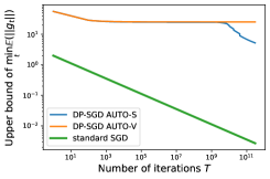
Here $\cdots$ represents the first argument of $\mathcal{G}$, and $\mathcal{G}$ is increasing and positive. As $T\to\infty$, we have $\min_{t}\mathbb{E}(\|\bm{g}_{t}\|)=O(T^{-1/4})$ for AUTO-S, the same rate as the standard SGD given in Theorem 9.

Figure 6: Left: DP-SGD with AUTO-V clipping. Middle: DP-SGD with AUTO-S clipping. Right: Log-log plot of convergence rate in comparison to standard SGD. Here $\xi=25,\gamma=0.01$, and the $O(1/\sqrt{T})$ term is set to 10 for DP-SGD and to 2 for standard SGD.

Remark 5.4.

We show in Theorem 6 and in Figure 6 that the upper bound (5.2) has $\mathcal{G}\geq\xi$ for AUTO-V ($\gamma=0$), and $\mathcal{G}$ only reduces to zero for AUTO-S ($\gamma>0$). We provide real data evidence in Figure 14 that strictly positive $\gamma$ reduces the gradient norm significantly.

5.2 Analysis of factors affecting the convergence

We now analyze the many factors that affect the convergence in Theorem 4, from a unified viewpoint of both the convergence and the privacy.

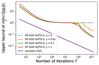
We start with the stability constant $\gamma$ and the learning rate $\eta_{t}$, both only affect the convergence not the privacy. We empirically observe in Figure 8 that small $\gamma$ benefits the convergence at initial iterations (when the privacy guarantee is strong) but larger $\gamma$ converges faster asymptotically. For $\eta_{t}$, the optimal is in fact the miminizer of the hyperbola in (C.5), that is unique and tunable.

Next, we focus on the hyperparameters that affect both convergence and privacy: the batch size $B$, the noise multiplier $\sigma$, and the number of iterations $T$. These hyperparameters have to be considered along the privacy-accuracy tradeoff, not just from a convergence perspective.

Recall that given a fixed privacy budget $(\epsilon,\delta)$, we rely on modern privacy accountant for computing the appropriate combinations of parameter $\sigma,T,B$. The exact expression of the bound as a function of $(\epsilon,\delta)$ is somewhat messy. For this reason, we illustrate our analysis in terms of the surrogate parameter $\mu$ for $\mu$-GDP [19], which implies $(\epsilon,\delta)$-DP with $\epsilon=\mu^{2}+\mu\sqrt{2\log(1/\delta)})$. [7] showed that DP-SGD’s privacy guarantee asymptotically converges to $\mu$-GDP (as $T\rightarrow\infty$) with $\mu=\frac{B}{n}\sqrt{T(e^{1/\sigma^{2}}-1)}$. We can alternatively leverage $\rho$-tCDP [10] for similar conclusions, using $\rho$ in place of $\mu^{2}$ in (5.3).

Theorem 5.

Under 5.1, 5.2, 5.3, fixing the asymptotic $\mu(\epsilon,\delta)$-GDP parameter, running DP-SGD with automatic clipping for $T$ iterations and setting the learning rate $\eta\propto 1/\sqrt{T}$ give

$$\min_{0\leq t\leq T}\mathbb{E}(\|\bm{g}_{t}\|) \leq\mathcal{G}\left(4\sqrt{(\mathcal{L}_{0}-\mathcal{L}_{*})L\left(\frac{1}{T}+\frac{d}{\mu^{2}n^{2}}+O\big{(}\frac{1}{B^{2}T}\big{)}\right)};\xi,\gamma\right)$$ (5.3)

To show that our analysis matches the training behaviors observed in SOTA empirical work [41, 38, 17, 68, 50, 78], we minimize the first argument of $\mathcal{G}$ in (5.3), denoted as $X(B,T,\mu,d,L,\mathcal{L}_{0})$.

1. [Train longer with larger noise] Fixing the expected batch size $B$, we see that $X$ is decreasing in $T$. Hence larger $T$ and consequently larger $\sigma$ are preferred.

2. [Larger batch size helps] Fixing number of iterations $T$ or epochs $E=BT/n$, we see that $X$ is decreasing in $B$. Hence larger $B$ and consequently larger $\sigma$ are preferred.

3. [Pretraining is critical] Pretraining can boost the DP accuracy through a much smaller initial loss $\mathcal{L}_{0}$ and from a smooth (small $L$) and flat (small $\xi$, c.f. Figure 8(left)) initialization.

4. [Learning rate needs tuning] The optimal learning rate by minimizing (C.5) is $\sqrt{\frac{(\mathcal{L}_{0}-\mathcal{L}_{*})\mu^{2}n^{2}}{L(\mu^{2}n^{2}+dT)}}$. This indicates that one should use larger learning rate for smaller model $d$, weaker privacy (larger $\mu$ or small $\epsilon$), or smaller iteration budget $T$.

6 Experiments

We evaluate our automatic DP training on image classification, sentence classification, and table-to-text generation tasks. Detailed settings including hyperparameters can be found in Appendix G.

6.1 Image classification

For MNIST/FashionMNIST, we use the same setup as in [56, 68, 64] with a simple CNN. For CIFAR10, we use the same setup as in [68] with pretrained SimCLRv2 [13]. For ImageNette, a 10-class sub-task of ImageNet [18], we use the same setup as in [36] without the learning rate decay. For CelebA [45], the real human face dataset, we train ResNet9 [32] with group normalization to replace the batch normalization. Notice that CelebA contains high-resolution (178x218) images, each with 40 labels. We consider CelebA for either multi-class classification on one label, e.g. ‘Smiling’ and ‘Male’, or for multi-label/multi-task problem to learn all labels simultaneously.

Table 1: Average test accuracy and 95% confidence interval on image tasks over 5 runs.

Task	Model	$(\epsilon,\delta)$	Accuracy %
			Abadi’s clipping	AUTO-S clipping	non-DP
					($\epsilon=\infty$)
MNIST	4-layer CNN	$(3,1e$-$5)$	$98.04\pm 0.09$	$98.15\pm 0.07$	$99.11\pm 0.07$
FashionMNIST	4-layer CNN	$(3,1e$-$5)$	$86.04\pm 0.26$	$86.36\pm 0.18$	$89.57\pm 0.13$
CIFAR10 pretrained	SimCLRv2	$(2,1e$-$5)$	$92.44\pm 0.13$	$92.70\pm 0.02$	$94.42\pm 0.01$
ImageNette	ResNet9	$(8,1e$-$4)$	$60.29\pm 0.53$	$60.71\pm 0.48$	$71.11\pm 0.37$
CelebA [Smiling]	ResNet9	$(8,5e$-$6)$	$90.75\pm 0.11$	$91.08\pm 0.08$	$92.61\pm 0.20$
CelebA [Male]	ResNet9	$(8,5e$-$6)$	$95.54\pm 0.14$	$95.70\pm 0.07$	$97.90\pm 0.04$
CelebA Multi-label	ResNet9	$(3,5e$-$6)$	$86.81\pm 0.03$	$87.05\pm 0.01$	$90.30\pm 0.02$
CelebA Multi-label	ResNet9	$(8,5e$-$6)$	$87.52\pm 0.15$	$87.58\pm 0.04$	$90.30\pm 0.02$

In Table 1, we observe that AUTO-S clipping outperforms existing clipping in all datasets with statistical significance. Interestingly, the standard deviation from different runs is smaller for automatic DP optimizers, indicating better reproducibility and stability. We additionally experiment 40 binary classification problems on CelebA with respect to each label, and observe that the mean accuracy further improves to 91.63% at $\epsilon=8$ for AUTO-S (see Appendix J).

6.2 Sentence classification

On five benchmark language datasets (MNLI(m/mm)[72], QQP[34], QNLI[62], SST2[67]), we compare our automatic DP training with re-parameterized gradient perturbation (RGP, [78]) and full-parameter finetuning (full, [41]) using RoBERTa models [44]. These methods use the same experimental setup. For language models, our automatic training is based on the codebase of [41].

Table 2: Test accuracy on language tasks with RoBERTa-base (12 blocks, 125 million parameters).

Method	$\epsilon=3$				$\epsilon=8$				$\epsilon=\infty$ (non-DP)
	MNLI	QQP	QNLI	SST2	MNLI	QQP	QNLI	SST2	MNLI	QQP	QNLI	SST2
RGP [78]	-	-	-	-	80.5/79.6	85.5	87.2	91.6	83.6/83.2	89.3	91.3	92.9
full [41]	82.45/82.99	85.56	87.42	91.86	83.20/83.46	86.08	87.94	92.09	85.91/86.14	87.34	91.40	94.49
full AUTO-V	81.21/82.03	84.72	86.56	91.86	82.18/82.64	86.23	87.24	92.09
full AUTO-S	83.22/83.21	85.76	86.91	92.32	83.82/83.55	86.58	87.85	92.43

Table 3: Test accuracy on language tasks with RoBERTa-large (24 blocks, 355 million parameters).

Method	$\epsilon=3$				$\epsilon=8$				$\epsilon=\infty$ (non-DP)
	MNLI	QQP	QNLI	SST2	MNLI	QQP	QNLI	SST2	MNLI	QQP	QNLI	SST2
RGP [78]	-	-	-	-	86.1/86.0	86.7	90.0	93.0	-	-	-	-
full [41]	86.43/86.46	86.43	90.76	93.04	87.02/87.26	87.47	91.10	93.81	90.33/90.03	87.90	93.61	96.21
full AUTO-V	85.33/85.61	86.61	89.99	93.12	85.91/86.10	86.86	90.55	93.35
full AUTO-S	86.27/86.67	86.76	91.01	93.92	87.07/87.16	87.47	91.45	94.61

In Table 3 and Table 3, we note that full parameter finetuning with AUTO-S outperforms or at least matches SOTA on all tasks. We use exactly the same hyperparameters as in [41].

6.3 Table-to-text generation

We compare our automatic DP training with a variety of fine-tuning methods, for table-to-text generation task on E2E dataset [23], where the goal is to generate texts about different aspects of a restaurant’s data. We measure the success on this task by BLEU, ROUGE-L (in Table 4), METEOR, NIST, CIDEr (extended in Table 8), with higher value meaning better model quality.

Table 4: Test performance on E2E dataset with GPT2. Additional performance measures are included in Table 8. The best two GPT2 models for each row are marked in bold.

	DP	GPT2	GPT2	GPT2
Metric	guarantee	large	medium
		full	full	full	full	full	LoRA	RGP	prefix	top2	retrain
		AUTO-S	AUTO-S	AUTO-S	AUTO-V	[41]	[33]	[78]	[40]
BLEU	$\epsilon=3$	64.180	63.850	61.340	61.519	61.519	58.153	58.482	47.772	25.920	15.457
	$\epsilon=8$	64.640	64.220	63.600	63.189	63.189	63.389	58.455	49.263	26.885	24.247
	non-DP	66.840	68.500	69.463	69.463	69.463	69.682	68.328	68.845	65.752	65.731
ROGUE-L	$\epsilon=3$	67.857	67.071	65.872	65.670	65.670	65.773	65.560	58.964	44.536	35.240
	$\epsilon=8$	68.968	67.533	67.073	66.429	66.429	67.525	65.030	60.730	46.421	39.951
	non-DP	70.384	71.458	71.359	71.359	71.359	71.709	68.844	70.805	68.704	68.751

Competitive methods include low-rank adaption (LoRA), prefix-tuning (prefix), RGP, only fine-tuning the top 2 Transformer blocks (top2), and training from scratch (retrain), as were recorded in [41]. Again, we use the exactly the same hyperparameters as in [41]. For GPT2 (124 million parameters), GPT2 medium (355 million), and GPT2 large (774 million), Table 4 shows that AUTO-S is scalable with stronger performance on larger models. Our automatic full-parameter finetuning has the best overall performance. Additionally, we highlight that AUTO-S and methods like LoRA are not mutually exclusive and can be combined to yield strong performance, since AUTO-S modifies the optimizers and LoRA modifies the architecture.

7 Related works

While other DP works also normalize the per-sample gradients (instead of clipping them) or use small clipping threshold (making the clipping similar to normalization), our work is very different in terms of theoretical analysis, algorithm design and experiments. In fact, the concurrent work [74] gives the same algorithm as AUTO-S, although its theoretical analysis and experiment design is fundamentally different from ours. [16] proposes to normalize the per-user (not per-sample) gradient in the federated learning setting, and analyzes the convergence in a convex, non-deep-learning setting.

On the other hand, many works apply the per-sample gradient clipping with small $R$ for good utility [1, 41, 50, 38, 17]. These works have led to valuable insights, but also some false or incomplete conclusions, due to the lack of rigorous theoretical analysis. For instance, since $R$ is present in the (re-parameterized) per-sample clipping, it cannot avoid the hyperparameter tuning as the choice of $R$ is not robust; even if a sufficiently small $R$ is used, the clipping does not reveal the stability constant in AUTO-S, which enjoys theoretical and empirical advantages in Remark 5.4 and Section 6. We devote Appendix L to more instances (e.g. Footnote 5) and a thorough comparison.

8 Discussion

In this work, we propose the automatic clipping as a drop-in replacement to the standard per-example clipping for differentially private training. This is the first technique that eliminates the need to tune the clipping threshold $R$, thus making DP deep learning as easy as regular learning. Our AUTO-S method enjoys both theoretical guarantee of convergence in non-convex problems (under various conditions), and strong empirical performance that advances DP learning on computer vision and language tasks.

We are excited about the future of automatic DP training, especially along with other working techniques, such as general optimizers (e.g. [8, 21]), clipping styles (all-layer or per-layer or adaptive clipping), architecture modifications (e.g. LoRA, RGP, prefix), and data augmentation (e.g. adversarial training [29] and multiple augmentation [17]). Thus, we expect to achieve comparable results to all SOTA in a lightweight fashion.

Appendix A Proof of differential privacy

Proof of Theorem 3.

Define the $\ell_{2}$ sensitivity of any function $g$ to be $\Delta g=\sup_{S,S^{\prime}}\|g(S)-g(S^{\prime})\|_{2}$ where the supreme is over all neighboring $(S,S^{\prime})$. Then the Gaussian mechanism $\hat{g}(S)=g(S)+\sigma\Delta g\cdot\mathcal{N}(0,\mathbf{I})$.

$\sigma$ denotes the “Noise multiplier”, which corresponds to the noise-level when a Gaussian mechanism is applied to a query with sensitivity $1$.

Observe that automatic clipping (AUTO-V and AUTO-S (4.1)) ensures the bounded global-sensitivity of the stochastic gradient as in Abadi’s clipping. Aligning the noise-multiplier (rather than the noise-level itself) ensures that the the noise-to-sensitivity ratio $\frac{\sigma\Delta g}{\Delta g}=\sigma$ is fixed regardless of $\Delta g$. The Gaussian mechanism’s privacy guarantees are equivalent. Thus from the privacy accountant perspective, DP-SGD with both Abadi’s clipping and our autoclipping method can be equivalently represented as the adaptive composition of $T$ Poisson sampled Gaussian Mechanism with sampling probability $B/n$ and noise multiplier $\sigma$. ∎

Appendix B Proof of automaticity

B.1 Non-adaptive DP optimizers

Proof of Theorem 1.

We prove Theorem 1 by showing that, DP-SGD using $R$-dependent AUTO-S with learning rate $\eta$ and weight decay $\lambda$ is equivalent to $R$-independent AUTO-S with learning rate $\eta R$ and weight decay $\lambda/R$. We claim other non-adaptive optimizers such as HeavyBall and NAG can be easily shown in a similar manner.

Recall the standard SGD with weight decay is

$$\bm{w}_{t+1}=\bm{w}_{t}-\eta\left(\sum_{i\in B_{t}}\frac{\partial l_{i}}{\partial\bm{w}_{t}}+\lambda\bm{w}_{t}\right)$$

Replacing the standard gradient $\sum_{i}\frac{\partial l_{i}}{\partial\bm{w}_{t}}$ with the private gradient, we write the $R$-dependent case as

$$\bm{w}_{t+1} =\bm{w}_{t}-\eta\left(\sum_{i\in B_{t}}\frac{\partial l_{i}}{\partial\bm{w}_{t}}\cdot R/\|\frac{\partial l_{i}}{\partial\bm{w}_{t}}\|_{2}+\sigma R\cdot\mathcal{N}(0,\mathbf{I})+\lambda\bm{w}_{t}\right)$$

$$=\bm{w}_{t}-\eta R\left(\sum_{i\in B_{t}}\frac{\partial l_{i}}{\partial\bm{w}_{t}}/\|\frac{\partial l_{i}}{\partial\bm{w}_{t}}\|_{2}+\sigma\cdot\mathcal{N}(0,\mathbf{I})\right)-\eta\lambda\bm{w}_{t}$$

which is clearly equivalent to the $R$-independent case:

$$\bm{w}_{t+1} =\bm{w}_{t}-\eta^{\prime}\left(\sum_{i\in B_{t}}\frac{\partial l_{i}}{\partial\bm{w}_{t}}/\|\frac{\partial l_{i}}{\partial\bm{w}_{t}}\|_{2}+\sigma\cdot\mathcal{N}(0,\mathbf{I})+\lambda^{\prime}\bm{w}_{t}\right)$$

if we use $\eta^{\prime}=\eta R$ and $\lambda^{\prime}=\lambda/R$. ∎

B.2 Adaptive DP optimizers

Proof of Theorem 2.

We prove Theorem 2 by showing that, DP-AdamW using $R$-dependent AUTO-S with learning rate $\eta$ and weight decay $\lambda$ is equivalent to $R$-independent AUTO-S with the same learning rate $\eta$ and weight decay $\lambda/R$. This is the most complicated case. We claim other adaptive optimizers such as AdaDelta, Adam with weight decay (not AdamW), and NAdam can be easily shown in a similar manner.

Recall the standard AdamW is

$$\bm{w}_{t+1}=\bm{w}_{t}-\eta\left(\frac{\mathbf{m}_{t}/(1-\beta_{1})}{\sqrt{\bm{v}_{t}/(1-\beta_{2})}}+\lambda\bm{w}_{t}\right)$$

where $\beta_{1},\beta_{2}$ are constants, $\bm{g}_{t}:=\sum_{i}\frac{\partial l_{i}}{\partial\bm{w}_{t}}$ is the standard gradient,

$$\mathbf{m}_{t}=\beta_{1}\mathbf{m}_{t-1}+(1-\beta_{1})\bm{g}_{t}\longrightarrow\mathbf{m}_{t}=\sum_{\tau}\beta_{1}^{t-\tau}(1-\beta_{1})\bm{g}_{\tau},$$

$$\bm{v}_{t}=\beta_{2}\bm{v}_{t-1}+(1-\beta_{2})\bm{g}_{t}^{2}\longrightarrow\bm{v}_{t}=\sum_{\tau}\beta_{2}^{t-\tau}(1-\beta_{2})\bm{g}_{\tau}^{2}.$$

Replacing the standard gradient with the private gradient $R\tilde{\bm{g}}_{t}:=R(\sum_{i}\frac{\partial l_{i}}{\partial\bm{w}_{t}}/\|\frac{\partial l_{i}}{\partial\bm{w}_{t}}\|_{2}+\sigma\cdot\mathcal{N}(0,I))$, we write the $R$-dependent DP-AdamW as

$$\bm{w}_{t+1}=\bm{w}_{t}-\eta\left(\frac{\tilde{\mathbf{m}}_{t}/(1-\beta_{1})}{\sqrt{\tilde{\bm{v}}_{t}/(1-\beta_{2})}}+\lambda\bm{w}_{t}\right)$$

where

$$\tilde{\mathbf{m}}_{t}=\beta_{1}\tilde{\mathbf{m}}_{t-1}+(1-\beta_{1})R\tilde{\bm{g}}_{t}\longrightarrow\tilde{\mathbf{m}}_{t}=\sum_{\tau}\beta_{1}^{t-\tau}(1-\beta_{1})R\tilde{\bm{g}}_{\tau},$$

$$\tilde{\bm{v}}_{t}=\beta_{2}\tilde{\bm{v}}_{t-1}+(1-\beta_{2})R^{2}\tilde{\bm{g}}_{t}^{2}\longrightarrow\tilde{\bm{v}}_{t}=\sum_{\tau}\beta_{2}^{t-\tau}(1-\beta_{2})R^{2}\tilde{\bm{g}}_{\tau}^{2}.$$

Clearly, the $R$ factor in the numerator and denominator of $\frac{\tilde{\mathbf{m}}_{t}/(1-\beta_{1})}{\sqrt{\tilde{\bm{v}}_{t}/(1-\beta_{2})}}$ cancel each other. Therefore we claim that the $R$-dependent DP-AdamW is in fact completely independent of $R$. ∎

B.3 Automatic per-layer clipping

In some cases, the per-layer clipping is desired, where we use a clipping threshold vector $\bm{R}=[R_{1},\cdots,R_{L}]$ and each layer uses a different clipping threshold. We claim that DP optimizers under automatic clipping works with the per-layer clipping when $\bm{R}$ is tuned proportionally, e.g. $\bm{R}=R\cdot[a_{1},\cdots,a_{L}]$, but not entry-wise (see counter-example in B.1). One special case is the uniform per-layer clipping when $R_{1}=\cdots=R_{L}=R/\sqrt{L}$. This is widely applied as only one norm $R$ requires tuning, instead of $L$ norms in $\bm{R}$, particularly in the case of deep models with hundreds of layers. The corresponding DP-SGD with AUTO-S in (3.5) gives

$$\bm{w}_{t+1}^{(l)}=\bm{w}_{t}^{(l)}-\eta\left(\sum_{i\in B_{t}}\frac{R}{\sqrt{L}}\frac{\bm{g}_{t,i}^{(l)}}{||\bm{g}_{t,i}^{(l)}||+\gamma}+\sigma R\cdot\mathcal{N}(0,\mathbf{I})\right)$$

Here the superscript $(l)$ is the layer index. Clearly $R$ couples with the learning rate $\eta$ and the same analysis as in Theorem 1 follows. The adaptive optimizers can be similarly analyzed from Theorem 2.

Fact B.1.

Changing one clipping threshold in the clipping threshold vector $\bm{R}$ (i.e. not proportionally) can break the coupling with learning rate.

Proof of B.1.

We prove by a counter-example of $\bm{R}$ in $\mathbb{R}^{2}$. Consider DP-SGD with per-layer clipping thresholds $(R_{1},R_{2})=(9,12)$:

$$\bm{w}_{t+1}^{(l)}=\bm{w}_{t}^{(l)}-\eta\left(\sum_{i\in B}\frac{R_{l}\bm{g}_{t,i,l}}{||\bm{g}_{t,i,l}||}+\sigma\sqrt{R_{1}^{2}+R_{2}^{2}}\cdot\mathcal{N}(0,\mathbf{I})\right)$$

Increasing $R_{1}$ from 9 to 16 changes the update for the first layer

$$\eta\left(\sum_{i\in B}\frac{9\bm{g}_{t,i,l}}{||\bm{g}_{t,i,l}||}+15\sigma\cdot\mathcal{N}(0,1)\right)\to\eta\left(\sum_{i\in B}\frac{16\bm{g}_{t,i,l}}{||\bm{g}_{t,i,l}||}+20\sigma\cdot\mathcal{N}(0,\mathbf{I})\right)$$

The noise-to-signal ratio decreases from 5/3 to 5/4 for this layer, and increases from 5/4 to 5/3 for the second layer. This breaks the coupling with learning rate, since the coupling does not change the noise-to-signal ratio. ∎

Appendix C Main results of convergence for DP-SGD with automatic clipping

C.1 Main proof of convergence for DP-SGD (the envelope version)

Proof of Theorem 4.

In this section, we prove two parts of Theorem 4.

The first part of Theorem 4 is the upper bound on $\min_{t}\mathbb{E}(\|\bm{g}_{t}\|)$, which is a direct result following from Theorem 6, and we prove it in Section C.2.

Theorem 6.

Under 5.1, 5.2, 5.3, running DP-SGD with automatic clipping for $T$ iterations gives

$$\min_{t}\mathbb{E}(\|\bm{g}_{t}\|)\leq\frac{\xi}{r}+\mathcal{F}\left(\frac{4}{\sqrt{T}}\sqrt{(\mathcal{L}_{0}-\mathcal{L}_{*})L\left(1+\frac{\sigma^{2}d}{B^{2}}\right)};r,\xi,\gamma\right)$$ (C.1)

where

• for $r<1,\gamma=0$ and $\eta\propto 1/\sqrt{T}$, $\mathcal{F}(x)=\frac{x}{\min_{0<c<1}f(c,r)}$ and $f(c,r):=\frac{(1+rc)}{\sqrt{r^{2}+2rc+1}}+\frac{(1-rc)}{\sqrt{r^{2}-2rc+1}}$; for $r\geq 1,\gamma=0$ and $\eta\propto 1/\sqrt{T}$, $\mathcal{F}(x)=\infty$;

• for $r\geq 1,\gamma>0$ and $\eta\propto 1/\sqrt{T}$, $\mathcal{F}$ is the convex envelope of (C.9), and is strictly increasing.

Figure 7: Visualization of upper bound $\frac{\xi}{r}+\mathcal{F}\left(O(1/\sqrt{T});r,\xi,\gamma\right)$ for gradient norm, with $O(1/\sqrt{T})$ in (C.1). Here $\xi=1$. The right plot is a zoom-in (with additional lines) of the left one.

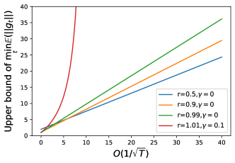
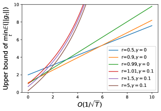
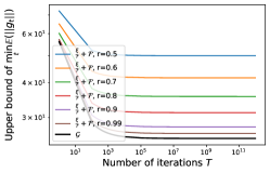
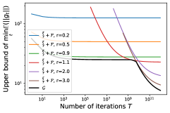
Notice that, (C.1) holds for any $r>0$. However, we have to consider an envelope curve over $r$ in (C.1) to reduce the upper bound: with AUTO-V clipping ($\gamma=0$), the upper bound in (C.1) is always larger than $\xi$ as $r<1$; we must use AUTO-S clipping ($\gamma>0$) to reduce the upper bound to zero, as can be seen from Figure 7. In fact, larger $T$ needs larger $r$ to reduce the upper bound.

All in all, we specifically focus on $r\geq 1$ and $\gamma>0$, which is the only scenario that (C.1) can converge to zero. This scenario is also where we prove the second part of Theorem 4.

The second part of Theorem 4 is the asymptotic convergence rate $O(T^{-1/4})$ of DP-SGD, only possible under $r\geq 1$ and $\gamma>0$.

By (C.1) in Theorem 6, our upper bound $\mathcal{G}$ from Theorem 4 can be simplified to

$$\min_{r>0}\frac{\xi}{r}+(\mathcal{M}^{-1})_{ccv}\left(\frac{4}{\sqrt{T}}\sqrt{(\mathcal{L}_{0}-\mathcal{L}_{*})L\left(1+\frac{\sigma^{2}d}{B^{2}}\right)};r,\xi,\gamma\right)$$

where the function $\mathcal{M}^{-1}$ is explicitly defined in (C.9) and the subscript $ccv$ means the upper concave envelope. Clearly, as $T\to\infty$, $\mathcal{M}^{-1}(\frac{1}{\sqrt{T}})\to 0$. We will next show that the convergence rate of $\mathcal{M}^{-1}$ is indeed $O(\frac{1}{\sqrt{T}})$ and the minimization over $r$ makes the overall convergence rate $O(T^{-1/4})$.

Starting from (C.9), we denote $x=\frac{4}{\sqrt{T}}\sqrt{(\mathcal{L}_{0}-\mathcal{L}_{*})L\left(1+\frac{\sigma^{2}d}{B^{2}}\right)}$ and write

$$\mathcal{M}^{-1}(x;r,\xi,\gamma) =\frac{-\frac{\xi}{r}\gamma+(r^{2}-1)\frac{\xi}{r}x+r\gamma x+\gamma\sqrt{(\frac{\xi}{r})^{2}+2\xi x+2\gamma x+x^{2}}}{2\gamma-(r^{2}-1)x}$$

$$=\left(-\frac{\gamma\xi}{r}+(r^{2}-1)\frac{\xi}{r}x+r\gamma x+\gamma\sqrt{(\frac{\xi}{r})^{2}+2\xi x+2\gamma x+x^{2}}\right)$$

$$\quad\cdot\frac{1+\frac{r^{2}-1}{2\gamma}x+O(x^{2})}{2\gamma}$$

$$=\frac{1}{2\gamma}\left(-\frac{\gamma\xi}{r}+(r^{2}-1)\frac{\xi}{r}x+r\gamma x+\frac{\gamma\xi}{r}\sqrt{1+\frac{2(\xi+\gamma)r^{2}x}{\xi^{2}}+O(x^{2})}\right)$$

$$\quad\cdot(1+\frac{r^{2}-1}{2\gamma}x+O(x^{2}))$$

$$=\frac{1}{2\gamma}\left(-\frac{\gamma\xi}{r}+(r^{2}-1)\frac{\xi}{r}x+r\gamma x+\frac{\gamma\xi}{r}\left(1+\frac{(\xi+\gamma)r^{2}x}{\xi^{2}}+O(x^{2})\right)\right)$$

$$\quad\cdot(1+\frac{r^{2}-1}{2\gamma}x+O(x^{2}))$$

$$=\frac{1}{2\gamma}\left((r^{2}-1)\frac{\xi}{r}x+r\gamma x+\frac{\gamma(\xi+\gamma)rx}{\xi}+O(x^{2})\right)\cdot(1+\frac{r^{2}-1}{2\gamma}x+O(x^{2}))$$

$$=\frac{1}{2\gamma}\left((r^{2}-1)\frac{\xi}{r}+r\gamma+\frac{\gamma(\xi+\gamma)r}{\xi}\right)\cdot x+O(x^{2})$$

$$=\frac{1}{2\gamma}\left(\frac{(\xi+\gamma)^{2}}{\xi}r-\frac{\xi}{r}\right)\cdot x+O(x^{2})$$

Since $\mathcal{M}^{-1}$ is asymptotically linear as $x\to 0$, we instead study

$$\min_{r>0}\frac{\xi}{r}+\mathcal{M}^{-1}\left(x;r,\xi,\gamma\right)\equiv\min_{r>0}\frac{\xi}{r}+\frac{1}{2\gamma}\left(\frac{(\xi+\gamma)^{2}}{\xi}r-\frac{\xi}{r}\right)\cdot x+O(x^{2}).$$

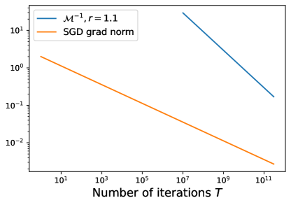
That is, ignoring the higher order term for the asymptotic analysis, the $\mathcal{M}^{-1}$ part converges as $O(x)=O(1/\sqrt{T})$, and we visualize this in Figure 9.

Although DP-SGD converges faster than SGD, the former converges to $\xi/r$ and the latter converges to 0. Thus, taking $\xi/r$ into consideration, the objective reduces to a hyperbola

$$\frac{\left(\xi(1-\frac{x}{2\gamma})\right)}{r}+\frac{x(\xi+\gamma)^{2}}{2\gamma\xi}\cdot r$$

whose minimum over $r$ is obviously $2\sqrt{\xi(1-\frac{x}{2\gamma})\frac{x(\xi+\gamma)^{2}}{2\gamma\xi}}=O(\sqrt{x})=O(T^{-1/4})$. ∎

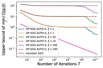
To give more details about the upper bound in (5.2), we demonstrate its dependence on $\xi$ and $\gamma$ in Figure 8.

Figure 8: Dependence of the upper bound $\mathcal{G}$ on $\xi$ (left) and $\gamma$ (right). Here the $O(1/\sqrt{T})$ term is set to 10 and either $\gamma=0.01$ (left) or $\xi=1$ (right).

Figure 9: Convergence with respect to $T$. Same setting as Figure 6.

C.2 Main proof of convergence for DP-SGD (the non-envelope version)

Proof of Theorem 6.

Consider DP-SGD with AUTO-S clipping

$$\bm{w}_{t+1}=\bm{w}_{t}-\eta\left(\sum_{i}\frac{\tilde{\bm{g}}_{t,i}}{\|\tilde{\bm{g}}_{t,i}\|+\gamma}+\sigma\mathcal{N}(0,\mathbf{I})\right)$$

where $\tilde{\bm{g}}_{t,i}$ is i.i.d. samples of $\tilde{\bm{g}}_{t}$, an unbiased estimate of $\bm{g}_{t}$, with a bounded variance as described in 5.3.

By Lipschitz smoothness in 5.2, and denoting $Z=\mathcal{N}(0,\mathbf{I})$, we have

$$\begin{split}\mathcal{L}_{t+1}-\mathcal{L}_{t}&\leq\bm{g}_{t}^{\top}(\bm{w}_{t+1}-\bm{w}_{t})+\frac{L}{2}\|\bm{w}_{t+1}-\bm{w}_{t}\|^{2}\\ &=-\eta\bm{g}_{t}^{\top}\left(\sum_{i}C_{i}\tilde{\bm{g}}_{t,i}+\sigma Z\right)+\frac{L\eta^{2}}{2}\left\|\sum_{i}C_{i}\tilde{\bm{g}}_{t,i}+\sigma Z\right\|^{2}\\ &\leq-\eta\bm{g}_{t}^{\top}\left(\sum_{i}C_{i}\tilde{\bm{g}}_{t,i}+\sigma Z\right)+L\eta^{2}\left(\left\|\sum_{i}C_{i}\tilde{\bm{g}}_{t,i}\right\|^{2}+\sigma^{2}\|Z\|^{2}\right)\\ &\leq-\eta\bm{g}_{t}^{\top}\left(\sum_{i}C_{i}\tilde{\bm{g}}_{t,i}+\sigma Z\right)+L\eta^{2}\left(B^{2}+\sigma^{2}\|Z\|^{2}\right)\end{split}$$ (C.2)

where the second last inequality follows from Cauchy Schwartz, and the last inequality follows from the fact that $\|C_{i}\tilde{\bm{g}}_{t,i}\|\leq 1$, e.g. $C_{i}$ is $\|\tilde{\bm{g}}_{t,i}/(\|\tilde{\bm{g}}_{t,i}\|+\gamma)\|$ or the re-parameterized clipping in [17].

Notice that in the last equality, the first term (ignoring $\bm{g}_{t}^{\top}Z$ for its zero expectation) can be written in the same form as (3.3), which supports our motivation in Section 3.2; the second term is independent of clipping functions. Note that the last inequality is tight if and only if $C_{i}=1$. This empirically holds in Section H.1, especially for GPT2.

Given the fact that $\|\tilde{\bm{g}}_{t,i}/(\|\tilde{\bm{g}}_{t,i}\|+\gamma)\|\leq 1$, the expected improvement at one iteration is

$$\begin{split}\mathbb{E}(\mathcal{L}_{t+1}-\mathcal{L}_{t}|\bm{w}_{t})&\leq-\eta\bm{g}_{t}^{\top}\mathbb{E}\left(\sum_{i}\frac{\tilde{\bm{g}}_{t,i}}{\|\tilde{\bm{g}}_{t,i}\|+\gamma}\right)+L\eta^{2}\left(B^{2}+\sigma^{2}d\right)\\ &=-\eta B\bm{g}_{t}^{\top}\mathbb{E}\left(\frac{\tilde{\bm{g}}_{t}}{\|\tilde{\bm{g}}_{t}\|+\gamma}\right)+L\eta^{2}\left(B^{2}+\sigma^{2}d\right)\end{split}$$ (C.3)

Now we want to lower bound $\bm{g}_{t}^{\top}\mathbb{E}\left(\frac{\tilde{\bm{g}}_{t}}{\|\tilde{\bm{g}}_{t}\|+\gamma}\right)$ in (C.3).

Write $\tilde{\bm{g}}_{t}=\bm{g}_{t}+\Delta_{t}$ where the gradient noise $\Delta_{t}$ follows $\mathbb{E}\Delta_{t}=0,\mathbb{E}\|\Delta_{t}\|<\xi$ by 5.3. Then

$$\bm{g}_{t}^{\top}\mathbb{E}\left(\frac{\tilde{\bm{g}}_{t}}{\|\tilde{\bm{g}}_{t}\|+\gamma}\right) =\mathbb{E}\left(\frac{\|\bm{g}_{t}\|^{2}+\bm{g}_{t}^{\top}\Delta_{t}}{\|\bm{g}_{t}+\Delta_{t}\|+\gamma}\right)$$

$$=\frac{1}{2}\mathbb{E}\left(\frac{\|\bm{g}_{t}\|^{2}+\bm{g}_{t}^{\top}\Delta_{t}}{\|\bm{g}_{t}+\Delta_{t}\|+\gamma}\Big{|}\Delta_{t}\in H_{+}\right)+\frac{1}{2}\mathbb{E}\left(\frac{\|\bm{g}_{t}\|^{2}+\bm{g}_{t}^{\top}\Delta_{t}}{\|\bm{g}_{t}+\Delta_{t}\|+\gamma}\Big{|}\Delta_{t}\in H_{-}\right)$$

$$=\frac{1}{2}\mathbb{E}\left(\frac{\|\bm{g}_{t}\|^{2}+\bm{g}_{t}^{\top}\Delta_{t}}{\|\bm{g}_{t}+\Delta_{t}\|+\gamma}\Big{|}\Delta_{t}\in H_{+}\right)+\frac{1}{2}\mathbb{E}\left(\frac{\|\bm{g}_{t}\|^{2}-\bm{g}_{t}^{\top}\Delta_{t}}{\|\bm{g}_{t}-\Delta_{t}\|+\gamma}\Big{|}\Delta_{t}\in H_{+}\right)$$

where we use the hyperplane perpendicular to $\bm{g}_{t}$ to divide the support of $\Delta_{t}$ into two half-spaces:

$$H_{+}:=\{\bm{v}:\bm{g}_{t}^{\top}\bm{v}>0\},\quad H_{-}:=\{\bm{v}:\bm{g}_{t}^{\top}\bm{v}<0\}.$$

We use the symmetry assumption in 5.3 to get

$$\mathbb{P}(\Delta_{t}\in H_{+})=\mathbb{P}(\Delta_{t}\in H_{-})=\frac{1}{2}$$

and notice that $\Delta_{t}\overset{D}{=}-\Delta_{t},$ i.e., if $\Delta_{t}\in H_{+}$, then $-\Delta_{t}\in H_{-}$ with the same distribution.

The next result further gives a lower bound for $\bm{g}_{t}^{\top}\mathbb{E}\left(\frac{\tilde{\bm{g}}_{t}}{\|\tilde{\bm{g}}_{t}\|+\gamma}\right)$ using $\|\bm{g}_{t}\|$.

Lemma C.1.

$$\mathbb{E}\left(\frac{\|\bm{g}_{t}\|^{2}+\bm{g}_{t}^{\top}\Delta_{t}}{\|\bm{g}_{t}+\Delta_{t}\|+\gamma}+\frac{\|\bm{g}_{t}\|^{2}-\bm{g}_{t}^{\top}\Delta_{t}}{\|\bm{g}_{t}-\Delta_{t}\|+\gamma}\Big{|}\Delta_{t}\in H_{+}\right)\geq\min_{0<c\leq 1}f(c,r;\frac{\gamma}{\|\bm{g}_{t}\|})\cdot(\|\bm{g}_{t}\|-\xi/r)$$

for any $r>0$ and $f(c,r;\Gamma)=\frac{(1+rc)}{\sqrt{r^{2}+2rc+1}+\Gamma}+\frac{(1-rc)}{\sqrt{r^{2}-2rc+1}+\Gamma}$.

For the simplicity of notation, we denote the distance measure

$$\mathcal{M}(\|\bm{g}_{t}\|-\xi/r;r,\xi,\gamma)=\min_{0<c\leq 1}f\left(c,r;\frac{\gamma}{\|\bm{g}_{t}\|}\right)\cdot(\|\bm{g}_{t}\|-\xi/r)$$ (C.4)

and leave the fine-grained analysis (e.g. its explicit form in some scenarios) at the end of this section.

Using the lower bound from Lemma C.1, the expected improvement (C.3) becomes

$$\mathbb{E}(\mathcal{L}_{t+1}-\mathcal{L}_{t}|\bm{w}_{t}) \leq-\frac{\eta B}{2}\mathcal{M}(\|\bm{g}_{t}\|-\xi/r)+L\eta^{2}B^{2}\left(1+\frac{\sigma^{2}d}{B^{2}}\right)$$

Now extend the expectation over randomness in the trajectory, and perform a telescoping sum over the iterations

$$\mathcal{L}_{0}-\mathcal{L}_{*} \geq\mathcal{L}_{0}-\mathbb{E}\mathcal{L}_{T}=\sum_{t}\mathbb{E}(\mathcal{L}_{t}-\mathcal{L}_{t+1})$$

$$\geq\frac{\eta B}{2}\mathbb{E}\left(\sum_{t}\mathcal{M}(\|\bm{g}_{t}\|-\xi/r)\right)-TL\eta^{2}B^{2}\left(1+\frac{\sigma^{2}d}{B^{2}}\right)$$

Substituting $\eta B=\eta_{\text{0}}/\sqrt{T}$ where $\eta_{\text{0}}$ is a base learning rate, we have

$$2(\mathcal{L}_{0}-\mathcal{L}_{*})\geq\sqrt{T}\eta_{\text{0}}\mathbb{E}\left(\frac{1}{T}\sum_{t}\mathcal{M}(\|\bm{g}_{t}\|-\xi/r)\right)-2L\eta^{2}_{\text{0}}\left(1+\frac{\sigma^{2}d}{B^{2}}\right)$$

and finally

$$\mathbb{E}\left(\frac{1}{T}\sum_{t}\mathcal{M}(\|\bm{g}_{t}\|-\xi/r)\right)\leq\frac{1}{\sqrt{T}}\left[\frac{2(\mathcal{L}_{0}-\mathcal{L}_{*})}{\eta_{\text{0}}}+2L\eta_{\text{0}}\left(1+\frac{\sigma^{2}d}{B^{2}}\right)\right]$$ (C.5)

With $\eta_{\text{0}}$ chosen properly at $\eta_{0}=\sqrt{\frac{\mathcal{L}_{0}-\mathcal{L}_{*}}{L\left(1+\frac{\sigma^{2}d}{B^{2}}\right)}}$, the hyperbola on the right hand side in (C.5) is minimized to $4\sqrt{(\mathcal{L}_{0}-\mathcal{L}_{*})L\left(1+\frac{\sigma^{2}d}{B^{2}}\right)}$, and we obtain

$$\mathbb{E}\left(\frac{1}{T}\sum_{t}\mathcal{M}(\|\bm{g}_{t}\|-\xi/r)\right)\leq\frac{4}{\sqrt{T}}\sqrt{(\mathcal{L}_{0}-\mathcal{L}_{*})L\left(1+\frac{\sigma^{2}d}{B^{2}}\right)}$$

Since the minimum of a sequence is smaller than the average, we have

$$\min_{t}\mathbb{E}(\mathcal{M}(\|\bm{g}_{t}\|-\xi/r))\leq\frac{1}{T}\sum_{t}\mathbb{E}\left(\mathcal{M}(\|\bm{g}_{t}\|-\xi/r)\right)\leq\frac{4}{\sqrt{T}}\sqrt{(\mathcal{L}_{0}-\mathcal{L}_{*})L\left(1+\frac{\sigma^{2}d}{B^{2}}\right)}$$ (C.6)

We claim that $\mathcal{M}$ may not be concave or convex. Therefore we use $\mathcal{M}_{cvx}$ to denote its lower convex envelope, i.e. the largest convex function that is smaller than $\mathcal{M}$. Then by Jensen’s inequality (C.6) becomes

$$\min_{t}\mathcal{M}_{cvx}(\mathbb{E}(\|\bm{g}_{t}\|-\xi/r))\leq\min_{t}\mathbb{E}(\mathcal{M}_{cvx}(\|\bm{g}_{t}\|-\xi/r))\leq\frac{4}{\sqrt{T}}\sqrt{(\mathcal{L}_{0}-\mathcal{L}_{*})L\left(1+\frac{\sigma^{2}d}{B^{2}}\right)}$$ (C.7)

It is obvious that $\mathcal{M}_{cvx}$ is increasing as $\mathcal{M}$ is increasing by Theorem 8. Hence, $(\mathcal{M}_{cvx})^{-1}$ is also increasing, as the inverse of $\mathcal{M}_{cvx}$. We write (C.7) as

$$\min_{t}\mathbb{E}(\|\bm{g}_{t}\|-\xi/r)\leq(\mathcal{M}_{cvx})^{-1}\left(\frac{4}{\sqrt{T}}\sqrt{(\mathcal{L}_{0}-\mathcal{L}_{*})L\left(1+\frac{\sigma^{2}d}{B^{2}}\right)}\right)$$

and equivalently

$$\min_{t}\mathbb{E}(\|\bm{g}_{t}\|)\leq\frac{\xi}{r}+(\mathcal{M}_{cvx})^{-1}\left(\frac{4}{\sqrt{T}}\sqrt{(\mathcal{L}_{0}-\mathcal{L}_{*})L\left(1+\frac{\sigma^{2}d}{B^{2}}\right)}\right)$$ (C.8)

Finally, we derive the explicit properties of $\mathcal{M}(\|\bm{g}_{t}\|-\xi/r)$ in Theorem 8. These properties allow us to further analyze on the convergence of $\mathcal{M}(\|\bm{g}_{t}\|-\xi/r)$, based on AUTO-V and AUTO-S, respectively.

1. DP-SGD with AUTO-V clipping.

By Theorem 8, we write

$$\mathcal{M}(x;r)=\min_{c\in(0,1]}f(c,r;0)\cdot x$$

This is a linear function and thus $\mathcal{M}_{cvx}=\mathcal{M}=1/\mathcal{M}_{cvx}^{-1}$. As a result, we have

$$\min_{t}\mathbb{E}(\|\bm{g}_{t}\|)\leq\frac{\xi}{r}+\frac{1}{\min_{c\in(0,1]}f(c,r;0)}\cdot\frac{4}{\sqrt{T}}\sqrt{(\mathcal{L}_{0}-\mathcal{L}_{*})L\left(1+\frac{\sigma^{2}d}{B^{2}}\right)}$$

We note here $r$ plays an important role under AUTO-V clipping: when $r<1$, we spend more iterations to converge to better and smaller gradient norm $\xi/r$; when $r\geq 1$, $\min_{c}f(c,r;0)=f(1,r;0)=0$ and it takes forever to converge. This is demonstrated in the left plot of Figure 6.

2. DP-SGD with AUTO-S clipping.

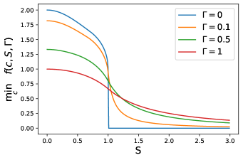
By Theorem 8 and for $r>1$, we write

$$\mathcal{M}(x;r,\xi,\gamma)=\left(\frac{\gamma}{(r-1)(x+\xi/r)+\gamma}-\frac{\gamma}{(r+1)(x+\xi/r)+\gamma}\right)\cdot x.$$

Notice that the inverse of a lower convex envelope is equivalent to the upper concave envelope (denoted by the subscript $ccv$) of an inverse. Therefore we can derive $(\mathcal{M}_{cvx})^{-1}=(\mathcal{M}^{-1})_{ccv}$ with the explicit form

$$\mathcal{M}^{-1}(x;r,\xi,\gamma)=\frac{-\frac{\xi}{r}\gamma+(r^{2}-1)\frac{\xi}{r}x+r\gamma x+\gamma\sqrt{(\frac{\xi}{r})^{2}+2\xi x+2\gamma x+x^{2}}}{2\gamma-(r^{2}-1)x}.$$ (C.9)

we can derive it based on $r,\xi,\gamma$ and substitute back to (C.8).

Note that the domain of $\mathcal{M}^{-1}$ (or the image of $\mathcal{M}$) is $[0,\frac{\gamma}{r-1}-\frac{\gamma}{r+1})$.

In comparison to the AUTO-V clipping, $\mathcal{M}^{-1}$ takes a much more complicated form, as depicted in the middle plot of Figure 6, where $r>1$ plays an important role for the gradient norm to converge to zero. ∎

C.3 Proof of Lemma C.1

Proof of Lemma C.1.

We want to lower bound

$$\mathbb{E}\left(\frac{\|\bm{g}_{t}\|^{2}+\bm{g}_{t}^{\top}\Delta_{t}}{\|\bm{g}_{t}+\Delta_{t}\|+\gamma}+\frac{\|\bm{g}_{t}\|^{2}-\bm{g}_{t}^{\top}\Delta_{t}}{\|\bm{g}_{t}-\Delta_{t}\|+\gamma}\Big{|}\Delta_{t}\in H_{+}\right)$$ (C.10)

To simplify the notation, we denote noise-to-signal ratio $S:=\frac{\|\Delta_{t}\|}{\|\bm{g}_{t}\|}$ and $c:=\cos\theta=\frac{\bm{g}_{t}^{\top}\Delta_{t}}{\|\bm{g}_{t}\|\|\Delta_{t}\|}$, with $\theta$ be the random angle between $\bm{g}_{t}$ and $\Delta_{t}$. Note that $0<c\leq 1$ when $\Delta_{t}\in H_{+}$.

The term inside the conditional expectation in (C.10) can be written as

$$\frac{(1+Sc)\|\bm{g}_{t}\|^{2}}{\sqrt{S^{2}+2Sc+1}\|\bm{g}_{t}\|+\gamma}+\frac{(1-Sc)\|\bm{g}_{t}\|^{2}}{\sqrt{S^{2}-2Sc+1}\|\bm{g}_{t}\|+\gamma}$$

$$= \|\bm{g}_{t}\|\left(\frac{(1+Sc)}{\sqrt{S^{2}+2Sc+1}+\gamma/\|\bm{g}_{t}\|}+\frac{(1-Sc)}{\sqrt{S^{2}-2Sc+1}+\gamma/\|\bm{g}_{t}\|}\right)$$

Defining $\Gamma=\gamma/\|\bm{g}_{t}\|$ and

$$f(c,S;\Gamma):=\frac{(1+Sc)}{\sqrt{S^{2}+2Sc+1}+\Gamma}+\frac{(1-Sc)}{\sqrt{S^{2}-2Sc+1}+\Gamma},$$ (C.11)

we turn the conditional expectation in (C.10) into

$$\mathbb{E}\left(\frac{\|\bm{g}_{t}\|^{2}+\bm{g}_{t}^{\top}\Delta_{t}}{\|\bm{g}_{t}+\Delta_{t}\|+\gamma}+\frac{\|\bm{g}_{t}\|^{2}-\bm{g}_{t}^{\top}\Delta_{t}}{\|\bm{g}_{t}-\Delta_{t}\|+\gamma}\Big{|}\Delta_{t}\in H_{+}\right)=\|\bm{g}_{t}\|\mathbb{E}(f(c,S;\Gamma)|\Delta_{t}\in H_{+})$$ (C.12)

for which we want to lower bound $f(c,S;\Gamma)$ over $0<c\leq 1,S>0,\Gamma>0$. We use the next theorem to prepare some helpful properties. The proof can be found in Section E.1.

Theorem 7.

For $f$ defined in (C.11), we have

1. $f(c,S;\Gamma)$ is strictly decreasing in $S$ for all $0<c<1$ and $\Gamma>0$.

2. Consequently, $\min_{c\in(0,1)}f(c,S;\Gamma)$ is strictly decreasing in $S$.

3. $f(c,S;\Gamma)$ is strictly decreasing in $c$ for all $S>1$ and $\Gamma>0$.

We consider a thresholding ratio $r>0$ and we will focus on the regime that $S<r$. This $r$ will turn out to measure the minimum gradient norm at convergence: informally speaking, $\|\bm{g}_{t}\|$ converges to $\xi/r$.

By the law of total expectation, (C.12) can be relaxed as follows.

$$\begin{split}&\|\bm{g}_{t}\|\mathbb{E}\left(f(c,S;\Gamma)\Big{|}\Delta\in H_{+}\right)\\ =&\|\bm{g}_{t}\|\mathbb{E}\left(f(c,S;\Gamma)\Big{|}\Delta\in H_{+},S<r\right)\mathbb{P}(r\|\bm{g}_{t}\|>\|\Delta\|\Big{|}\Delta\in H_{+})\\ &+\|\bm{g}_{t}\|\mathbb{E}\left(f(c,S;\Gamma)\Big{|}\Delta\in H_{+},S>r\right)\mathbb{P}(r\|\bm{g}_{t}\|<\|\Delta\|\Big{|}\Delta\in H_{+})\\ \geq&\|\bm{g}_{t}\|\mathbb{E}\left(f(c,S;\Gamma)\Big{|}\Delta\in H_{+},S<r\right)\mathbb{P}(r\|\bm{g}_{t}\|>\|\Delta\|\Big{|}\Delta\in H_{+})\\ \geq&\|\bm{g}_{t}\|\mathbb{E}\left(f(c,r;\Gamma)\Big{|}\Delta\in H_{+},S<r\right)\mathbb{P}(r\|\bm{g}_{t}\|>\|\Delta\|\Big{|}\Delta\in H_{+})\\ =&\|\bm{g}_{t}\|\mathbb{E}\left(f(c,r;\Gamma)\Big{|}\Delta\in H_{+},S<r\right)\mathbb{P}(r\|\bm{g}_{t}\|>\|\Delta\|)\\ \geq&\min_{c\in(0,1]}f(c,r;\Gamma)\cdot\underbrace{\|\bm{g}_{t}\|\mathbb{P}(r\|\bm{g}_{t}\|>\|\Delta\|)}_{$\star$⃝}\end{split}$$ (C.13)

where in the first inequality, the ignoring of last term is justified by $f(c,S;\Gamma)\geq\min_{c\in(0,1]}f(c,S;\Gamma)\geq\min_{c\in(0,1]}f(c,\infty;\Gamma)=0$, from the monotonicity (second statement) in Theorem 7.

We first lower bound $\star$⃝ by applying the Markov’s inequality:

$$\mathbb{P}(r\|\bm{g}_{t}\|>\|\Delta_{t}\|)\geq 1-\frac{\mathbb{E}\|\Delta_{t}\|}{r\|\bm{g}_{t}\|}$$

and hence by 5.3,

$$\|\bm{g}_{t}\|\mathbb{P}(r\|\bm{g}_{t}\|>\|\Delta_{t}\|)\geq\|\bm{g}_{t}\|-\mathbb{E}\|\Delta\|/r\geq\|\bm{g}_{t}\|-\xi/r.$$

Finally, the conditional expectation of interest in (C.10) gives

$$\mathbb{E}\left(\frac{\|\bm{g}_{t}\|^{2}+\bm{g}_{t}^{\top}\Delta_{t}}{\|\bm{g}_{t}+\Delta_{t}\|}+\frac{\|\bm{g}_{t}\|^{2}-\bm{g}_{t}^{\top}\Delta_{t}}{\|\bm{g}_{t}-\Delta_{t}\|}\Big{|}\Delta_{t}\in H_{+}\right)\geq\min_{0<c\leq 1}f(c,r;\frac{\gamma}{\|\bm{g}_{t}\|})\cdot(\|\bm{g}_{t}\|-\xi/r)$$

∎

C.4 Proof of Theorem 8

To derive some properties of $\min_{c}f(c,r;\Gamma)$, we need to compute separately for AUTO-V (without the stability constant, $\Gamma=0$) and for AUTO-S (with the stability constant, $\Gamma>0$), as shown in Theorem 8. As we will show, as the number of training iterations $T\to\infty$, DP-SGD with AUTO-V clipping can only compress $\|\bm{g}_{t}\|$ to $\xi/r$ for $r<1$. However, DP-SGD with AUTO-S clipping can compress $\|\bm{g}_{t}\|$ to $\xi/r$ to any $r>1$.

Theorem 8.

1. For $0<r<1$ and $\Gamma=0$, we have $\min_{c\in(0,1]}f(c,r;0)>0$. Then Equation C.12 is lower bounded by

   $$\min_{c\in(0,1]}f(c,r;0)\cdot(\|\bm{g}_{t}\|-\xi/r)$$

   which is increasing in $\|g\|-\xi/r$.

2. For $r\geq 1$ and $\Gamma=0$, we have $\min_{c\in(0,1]}f(c,r;\Gamma)=f(1,r;0)=0$. In words, (C.10) has a trivial lower bound and Theorem 6 cannot compress $\|\bm{g}_{t}\|$ to $\xi/r$.

3. For $r\geq 1$ and $\Gamma>0$, we have $\min_{c\in(0,1]}f(c,r;\Gamma)=f(1,r;\Gamma)=\left(\frac{\Gamma}{r+\Gamma-1}-\frac{\Gamma}{r+\Gamma+1}\right)$. Then Equation C.12 is lower bounded by

   $$\left(\frac{\gamma}{(r-1)\|\bm{g}_{t}\|+\gamma}-\frac{\gamma}{(r+1)\|\bm{g}_{t}\|+\gamma}\right)\cdot(\|\bm{g}_{t}\|-\xi/r)$$

   which is increasing in $\|\bm{g}_{t}\|-\xi/r$.

Proof.

To prove statement 1, we use the second statement from Theorem 7 and show that $\min_{c}f(c,r;0)>\min_{c}f(c,\infty;0)=0$. To prove statement 2 and 3, we use the third statement from Theorem 7 and see that $\min_{c}f(c,r;\Gamma)=f(1,r;\Gamma)$ with an explicit formula. ∎

Appendix D Convergence rate of standard SGD

Theorem 9.

Under 5.1, 5.2, 5.3 (without the symmetry assumption), running the standard non-DP SGD for $T$ iterations gives, for $\eta\propto 1/\sqrt{T}$,

$$\min_{t}\mathbb{E}\left(\|\bm{g}_{t}\|\right)\leq\frac{1}{T^{1/4}}\sqrt{2(\mathcal{L}_{0}-\mathcal{L}_{*})L+\frac{\xi^{2}}{B}}$$

Proof of Theorem 9.

Consider the standard SGD

$$\bm{w}_{t+1}=\bm{w}_{t}-\eta\frac{\sum_{i}\tilde{\bm{g}}_{t,i}}{B}$$

where $\tilde{\bm{g}}_{t,i}$ is i.i.d. unbiased estimate of $\bm{g}_{t}$, with a bounded variance as described in 5.3.

By Lipschitz smoothness assumption in 5.2,

$$\mathcal{L}_{t+1}-\mathcal{L}_{t} \leq\bm{g}_{t}^{\top}(\bm{w}_{t+1}-\bm{w}_{t})+\frac{L}{2}\|\bm{w}_{t+1}-\bm{w}_{t}\|^{2}=-\eta\bm{g}_{t}^{\top}\left(\sum_{i}\frac{1}{B}\tilde{\bm{g}}_{t,i}\right)+\frac{L\eta^{2}}{2}\left\|\sum_{i}\frac{1}{B}\tilde{\bm{g}}_{t,i}\right\|^{2}$$

The expected improvement at one iteration is

$$\begin{split}\mathbb{E}(\mathcal{L}_{t+1}-\mathcal{L}_{t}|\bm{w}_{t})&\leq-\eta\bm{g}_{t}^{\top}\mathbb{E}\tilde{\bm{g}}_{t,i}+\frac{L\eta^{2}}{2}\mathbb{E}\|\sum_{i}\frac{1}{B}\tilde{\bm{g}}_{t,i}\|^{2}\\ &\leq-\eta\|\bm{g}_{t}\|^{2}+\frac{L\eta^{2}}{2}\left(\|\bm{g}_{t}\|^{2}+\frac{\xi^{2}}{B}\right)\end{split}$$ (D.1)

Now we extend the expectation over randomness in the trajectory, and perform a telescoping sum over the iterations

$$\mathcal{L}_{0}-\mathcal{L}_{*} \geq\mathcal{L}_{0}-\mathbb{E}\mathcal{L}_{T}=\sum_{t}\mathbb{E}(\mathcal{L}_{t}-\mathcal{L}_{t+1})\geq\left(\eta-\frac{L\eta^{2}}{2}\right)\mathbb{E}(\sum_{t}\|\bm{g}_{t}\|^{2})-\frac{TL\eta^{2}\xi^{2}}{2B}$$

Notice that we do not need the symmetry assumption in 5.3 in the non-DP SGD analysis.

We apply the same learning rate as in [5], $\eta=\frac{1}{L\sqrt{T}}$,

$$2(\mathcal{L}_{0}-\mathcal{L}_{*})\geq\left(\frac{2}{L\sqrt{T}}-\frac{1}{LT}\right)\mathbb{E}\left(\sum_{t}\|\bm{g}_{t}\|^{2}\right)-\frac{T\xi^{2}}{BLT}\geq\frac{\sqrt{T}}{L}\mathbb{E}\left(\frac{1}{T}\sum_{t}\|\bm{g}_{t}\|^{2}\right)-\frac{\xi^{2}}{BL}$$

and finally

$$\min_{t}\mathbb{E}\left(\|\bm{g}_{t}\|^{2}\right)\leq\mathbb{E}\left(\frac{1}{T}\sum_{t}\|\bm{g}_{t}\|^{2}\right)\leq\frac{1}{\sqrt{T}}\left[2(\mathcal{L}_{0}-\mathcal{L}_{*})L+\frac{\xi^{2}}{B}\right]$$

Using the Jensen’s inequality, we can have

$$\min_{t}\mathbb{E}\left(\|\bm{g}_{t}\|\right)\leq\frac{1}{T^{1/4}}\sqrt{2(\mathcal{L}_{0}-\mathcal{L}_{*})L+\frac{\xi^{2}}{B}}$$

∎

Appendix E Auxiliary proofs

E.1 Proof of Theorem 7

Proof.

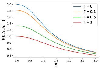
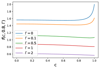
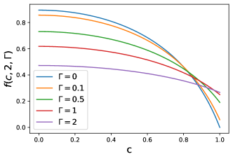
We first show $\frac{df(c,S;\Gamma)}{dS}<0$ for all $0<c<1,\Gamma>0$ and $S>0$, as visualized in the left plot of Figure 10. We can explicitly write down the derivative, by WolframAlpha

$$\frac{df(c,S;\Gamma)}{dS}=\frac{-(A\Gamma^{2}+B\Gamma+C)}{\sqrt{S^{2}-2cS+1}\sqrt{S^{2}+2cS+1}(\Gamma+\sqrt{S^{2}-2cS+1})^{2}(\Gamma+\sqrt{S^{2}+2cS+1})^{2}}$$ (E.1)

with

$$A(c,S) =\sqrt{S^{2}+2cS+1}\left(3c^{2}S-2c(S^{2}+1)+S\right)+\sqrt{S^{2}-2cS+1}\left(3c^{2}S+2c(S^{2}+1)+S\right)$$

$$B(c,S) =4S\left[(S^{2}+1)(1-c^{2})+c^{2}\sqrt{S^{2}+2cS+1}\sqrt{S^{2}-2cS+1}\right]$$

$$C(c,S) =(1-c^{2})S\left[(S^{2}-2cS+1)^{3/2}+(S^{2}+2cS+1)^{3/2}\right]$$

It is obvious that, since $c<1$,

$$S^{2}\pm 2cS+1>S^{2}\pm 2cS+c^{2}=(S\pm c)^{2}\geq 0.$$ (E.2)

From (E.2), the denominator in (E.1) is positive and it suffices to show $A\Gamma^{2}+B\Gamma+C>0$ for all $0<c<1$ and $S>0$, in order to show $\frac{df}{dS}<0$.

Also from (E.2), we can easily see $B(c,S)>0$ and $C(c,S)>0$. We will show that $A(c,S)>0$ in Lemma E.1, after very heavy algebraic computation.

Now we can claim that $A\Gamma^{2}+B\Gamma+C>0$ by E.3, and complete the proof of the first statement.

To further see that $\min_{c}f(c,S;\Gamma)$ is decreasing in $S$, let us denote $c^{*}(x;\Gamma):=\text{arg min}_{c\in[0,1]}f(c,x;\Gamma)$. Then considering $S<S^{\prime}$, we prove the second statement by observing

$$\min_{c}f(c,S;\Gamma)=f(c^{*}(S;\Gamma),S;\Gamma)>f(c^{*}(S;\Gamma),S^{\prime};\Gamma)\geq\min_{c}f(c,S^{\prime};\Gamma).$$

This statement is also visualized in the right plot of Figure 10.

We next show $\frac{df(c,S;\Gamma)}{dc}<0$ for all $0<c<1,\Gamma>0$ and $S>1$. We can explicitly write down the derivative, by WolframAlpha

$$\frac{df(c,S;\Gamma)}{dc}=\frac{-S(A^{\prime}\Gamma^{2}+B^{\prime}\Gamma+C^{\prime})}{\sqrt{S^{2}-2cS+1}\sqrt{S^{2}+2cS+1}(\Gamma+\sqrt{S^{2}-2cS+1})^{2}(\Gamma+\sqrt{S^{2}+2cS+1})^{2}}$$ (E.3)

with

$$A^{\prime}(c,S) =\left[(S^{2}+3cS+2)\sqrt{S^{2}-2cS+1}-(S^{2}-3cS+2)\sqrt{S^{2}+2cS+1}\right]$$

$$B^{\prime}(c,S) =4Sc\left[\sqrt{S^{2}+2cS+1}\sqrt{S^{2}-2cS+1}+(S^{2}-1)\right]$$

$$C^{\prime}(c,S) =S\left[(c+S)(S^{2}-2cS+1)^{3/2}+(c-S)(S^{2}+2cS+1)^{3/2}\right]$$

Clearly $B^{\prime}(c,S)>0$ and $C^{\prime}(c,S)>0$, since $S^{2}+2cS+1>S^{2}-2cS+c^{2}=(S-c)^{2}\geq 0$. And we will show $A^{\prime}(c,S)>0$ in Lemma E.2, after some algebra.

We again claim that $A^{\prime}\Gamma^{2}+B^{\prime}\Gamma+C^{\prime}>0$ by E.3, which guarantees that the numerator in (E.3) is negative and that $\frac{df}{dc}<0$. This is visualized in Figure 11. ∎

Figure 10: Visualization of $f(0.5,S,\Gamma)$ (left) and $\min_{0\leq c\leq 1}f(c,S,\Gamma)$ over $S>0$.

Figure 11: Visualization of $f(c,0.8,\Gamma)$ (left) and $f(c,2,\Gamma)$ over $0\leq c\leq 1$.

E.2 Proof of Lemma E.1

Lemma E.1.

For all $0<c<1$ and $S>0$,

$$A:=\sqrt{S^{2}+2cS+1}\left(3c^{2}S-2c(S^{2}+1)+S\right)+\sqrt{S^{2}-2cS+1}\left(3c^{2}S+2c(S^{2}+1)+S\right)>0.$$

Proof.

We prove by contradiction. Suppose

$$\sqrt{S^{2}+2cS+1}\left(3c^{2}S-2c(S^{2}+1)+S\right)+\sqrt{S^{2}-2cS+1}\left(3c^{2}S+2c(S^{2}+1)+S\right)<0.$$

Then

$$0<\sqrt{S^{2}-2cS+1}\left(3c^{2}S+2c(S^{2}+1)+S\right)<-\sqrt{S^{2}+2cS+1}\left(3c^{2}S-2c(S^{2}+1)+S\right).$$

where the first inequality comes from $S^{2}-2cS+1>S^{2}-2cS+c^{2}=(S-c)^{2}\geq 0$.

Squaring everything gives

$$(S^{2}-2cS+1)\left(3c^{2}S+2c(S^{2}+1)+S\right)^{2}<(S^{2}+2cS+1)\left(3c^{2}S-2c(S^{2}+1)+S\right)^{2}.$$

Taking the difference gives

$$4cS(2+3S^{2}-9c^{4}S^{2}+2S^{4}+2c^{2}(1-S^{2}+S^{4}))<0$$

Given that $c>0,S>0$, we have

$$2+3S^{2}-9c^{4}S^{2}+2S^{4}+2c^{2}(1-S^{2}+S^{4})<0$$

Denoting $X:=S^{2}$ and viewing the above as a quadratic polynomial of $X$, we have

$$\underbrace{(2c^{2}+2)X^{2}+(3-2c^{2}-9c^{4})X+(2c^{2}+2)}_{①}<0$$

Using the closed-form minimizer of quadratic polynomial $①$, after some heavy algebra, one can check the minimum of $①$ is

$$\frac{(1+3c^{2})^{2}(1-c^{2})(7+9c^{2})}{8(1+c^{2})}$$

which is clearly positive. Contradiction! ∎

E.3 Proof of Lemma E.2

Lemma E.2.

For all $0<c<1$ and $S>1$,

$$(S^{2}+3cS+2)\sqrt{S^{2}-2cS+1}-(S^{2}-3cS+2)\sqrt{S^{2}+2cS+1}>0.$$

Proof.

Notice that $(S^{2}+3cS+2)>S^{2}+2>0$ and $\sqrt{S^{2}\pm 2cS+1}>0$. Therefore if $S^{2}-3cS+2\leq 0$, we are done.

Otherwise, we prove by contradiction and suppose

$$0<(S^{2}+3cS+2)\sqrt{S^{2}-2cS+1}<(S^{2}-3cS+2)\sqrt{S^{2}+2cS+1}.$$

under the condition that $S^{2}-3cS+2>0$.

Squaring everything gives

$$(S^{2}+3cS+2)^{2}(S^{2}-2cS+1)<(S^{2}-3cS+2)^{2}(S^{2}+2cS+1).$$

Taking the difference gives

$$cS(8+20S^{2}-36c^{2}S^{2}+8S^{4})<0$$

Given that $c>0,S>0$, we have

$$2+5S^{2}-9c^{2}S^{2}+2S^{4}<0$$

Denoting $X:=S^{2}$ and viewing the above as a quadratic polynomial of $X$, we have, for $X>1$,

$$\underbrace{2X^{2}+(5-9c^{2})X+2}_{②}<0$$

The closed-form minimizer of quadratic polynomial $②$ is $\frac{(9c^{2}-5)}{4}$. Given that $0<c<1$, we must have $-\frac{5}{4}<\frac{9c^{2}-5}{4}<1$. Hence the minimizer is not within the feasible domain $(1,\infty)$ of $X$. Thus the minimum of ② is achieved with $X=1$ at $9(1-c^{2})$. This is positive. Contradiction! ∎

E.4 Proof of E.3

Fact E.3.

For a quadratic polynomial $Ax^{2}+Bx+C$ with $A,B,C>0$, the minimum value on the domain $x\geq 0$ is $C$, at $x=0$. Therefore $Ax^{2}+Bx+C>0$.

Proof.

Since $A>0$, the quadratic polynomial is convex and increasing on the domain $x>-\frac{B}{2A}$. Since $B>0$ as well, we know $-\frac{B}{2A}<0$ and hence the quadratic polynomial is strictly increasing on $x>0$. Therefore the minimum value is achieved when $x=0$, and we obtain $Ax^{2}+Bx+C\geq C>0$ for all $x\geq 0$. ∎

E.5 Assumption of symmetric gradient noise

We show that 5.3 is actually relaxed from and less strict than the assumptions used in the non-DP literature. In words, 5.3 allows our DP convergence to be comparable to the standard convergence (as in Theorem 9), because our assumption does not enforce extra constraint.

In standard non-DP analysis [48, 66, 12, 73], the mini-batch gradient is assumed to be an unbiased estimate of the oracle gradient $\bm{g}_{t}=\frac{\partial\mathcal{L}}{\partial\bm{w}}$:

$$\frac{1}{B}\sum_{i=1}^{B}\tilde{\bm{g}}_{t,i}\sim\bm{g}_{t}+\bm{\xi}(\bm{w})$$

and $\bm{\xi}$ is the random gradient noise with $\bm{\xi}\sim N(\bm{0},\Sigma(\bm{w})/B)$. Since this assumption holds for any batch size $B$, we can set $B=1$ to recover the per-sample gradient noise: $\bm{\xi}=\tilde{\bm{g}}_{t,i}-\bm{g}_{t}$ is i.i.d. and symmetric because a zero-mean Gaussian is symmetric.

In fact, we can further relax our 5.3: besides assuming the central symmetry, the same proof of convergence will follow if we instead assume the mirror symmetry about the hyperplane normal to $\bm{g}_{t}$, that is $\{\bm{v}:\bm{g}_{t}^{\top}\bm{v}=0\}$.

Appendix F Examples of lazy regions

F.1 Balanced binary classification

We describe the data generation in Section 3.3. The label is uniformly $\pm 1$, that is $\mathbb{P}(y_{i}=+1)=\mathbb{P}(y_{i}=-1)=0.5$. We have 10000 positive and negative samples $x_{i}\sim\mathcal{N}(y_{i},1)$. We consider a logistic regression model $\mathbb{P}(Y=y|x)=\mathbb{I}(y=1)\cdot\text{Sigmoid}(x+\theta)+\mathbb{I}(y=-1)\cdot(1-\text{Sigmoid}(x+\theta))=\frac{1}{1+e^{-y(\theta+x)}}$, where $\theta\in\mathbb{R}$ is the intercept. The gradient with respect to this only trainable parameter is $\frac{\partial\mathcal{L}_{i}}{\partial\theta}=-y\left(1-\frac{1}{1+e^{-y(\theta+x)}}\right)$. We set the clipping threshold $R=0.01$ and the stability constant $\gamma=0.01$.

F.2 Mean estimation on Gaussian mixture data

We also observe the lazy region issue in the mean estimation problem $\min_{\theta}\frac{1}{2}\|\theta-x_{i}\|^{2}$. Here $\mathbb{P}(x_{i}\sim\mathcal{N}(4,1))=\mathbb{P}(x_{i}\sim\mathcal{N}(4,1))=0.5$. We have 10000 samples from each Gaussian distribution. The regular minimum is clearly $\sum_{i}x_{i}\to 0$, where the regular gradient and AUTO-S clipped gradient vanish. Yet both AUTO-V and Abadi’s clipping lose motivation to update the mean estimator on the interval $(-1,1)$. We set the clipping threshold $R=0.01$ and the stability constant $\gamma=0.1$.

Figure 12: Scalar gradient $\frac{\partial\mathcal{L}}{\partial\theta}$ at each $\theta$.

Appendix G Experiments settings

G.1 Image classification settings

We give the experiments settings for computer vision tasks in Table 1.

• MNIST: We use the network architecture from [56, 68, 64], with 40 epochs, 512 batch size, 0.5 learning rate (or 0.005 non-DP learning rate), 0.1 clipping threshold, DP-SGD with 0.9 momentum, and without pretraining. This setting is the same as [68].

• FashionMNIST: We use the same network architecture as MNIST, with 40 epochs, 2048 batch size, 4 learning rate (or 0.04 non-DP learning rate), DP-SGD with 0.9 momentum, and without pretraining. This setting is the same as [68].

• CIFAR10 pretrained: We use the SimCLR model from [13], with 50 epochs, 1024 batch size, 4 learning rate (or 0.04 non-DP learning rate), 0.1 clipping threshold, and DP-SGD with 0.9 momentum. The SimCLR model is pretrained on unlabelled ImageNet dataset. After pretraining, we obtain a feature of dimension 4096 on which a linear classifier is trained privately. This setting is the same as [68].

• ImageNette: We use the ResNet9 (2.5 million parameters) with Mish activation function [52]. We set 50 epochs, 1000 batch size, 0.0005 learning rate (or 0.000005 non-DP learning rate), 1.5 clipping threshold, and use DP-NAdam, without pretraining. This setting is the same as [36] except we did not apply the learning rate decaying scheduler.

• CelebA (Smiling and Male and Multi-label) We use the same ResNet9 as above, with 10 epochs, 500 batch size, 0.001 DP learning rate (or 0.00001 non-DP learning rate), 0.1 clipping threshold, and use DP-Adam, without pretraining. We use the labels ‘Smiling’ and ‘Male’ for two binary classification tasks, with cross-entropy loss. For the multi-label task uses a scalar loss by summing up the 40 binary cross-entropy losses from each label.

We refer the code for MNIST, FashionMNIST, CIFAR10, CIFAR10 pretrained to https://github.com/ftramer/Handcrafted-DP by [68]. ResNet9 can be found in https://github.com/cbenitez81/Resnet9.

Throughout all experiments, we do not apply tricks such as random data augmentation (single or multiple times [17]), weight standardization [61], or parameter averaging [60].

G.2 Sentence classification settings

We experiment on five datasets in Table 3 and Table 3.

• MNLI(m) MNLI-matched, the matched validation and test splits from Multi-Genre Natural Language Inference Corpus.

• MNLI(mm) MNLI-mismatched, the matched validation and test splits from Multi-Genre Natural Language Inference Corpus.

• QQP The Quora Question Pairs2 dataset.

• QNLI The Stanford Question Answering dataset.

• SST2 The Stanford Sentiment Treebank dataset.

The datasets are processed and loaded from Huggingface [39], as described in https://huggingface.co/datasets/glue. We follow the same setup as [78] and [41]. We refer the interested readers to Appendix G,H,I,K,N of [41] for more details.

We emphasize that our automatic clipping uses exactly the same hyperparameters as the Abadi’s clipping in [41], which is released in their Private-Transformers library .

Dataset	MNLI(m/mm)	QQP	QNLI	SST2
Epoch	18	18	6	3
Batch size	6000	6000	2000	1000
clipping threshold $R$	0.1	0.1	0.1	0.1
DP learning rate	5e-4	5e-4	5e-4	5e-4
non-DP learning rate	5e-5	5e-5	5e-5	5e-5
learning rate decay	Yes	Yes	Yes	Yes
AdamW weight decay	0	0	0	0
Max sequence length	256	256	256	256

Table 5: Hyperparameters of automatic clipping and Abadi’s clipping, for sentence classification in Table 3 and Table 3, using either RoBERTa base or large.

Notice that we use DP learning rate 5e-4 across tasks for the $R$-dependent automatic DP-Adam, which is equivalent to $R$-independent automatic DP-Adam with the same learning rate. We demonstrate that the results are not sensitive to learning rates around the optimal choice. That is, the automatic clipping does not eliminate $R$ at the cost of more difficult tuning of learning rate.

learning rate	1e-4	3e-4	5e-4	8e-4	1e-3
RoBERTa-base	93.92	94.38	94.49	94.72	93.35
RoBERTa-large	95.76	96.21	96.21	96.33	95.99

Table 6: SST2 accuracy with respect to learning rate.

G.3 Table-to-text generation settings

We experiment multiple GPT2 models on E2E dataset from Huggingface [39] in Table 4. We follow the same setup as [41], and our automatic clipping uses exactly the same hyperparameters as the Abadi’s clipping in [41], which is released in their Private-Transformer library .

Model	GPT2	GPT2 medium	GPT2 large
Epoch	10	10	10
Batch size	1024	1024	1024
clipping threshold $R$	0.1	0.1	0.1
DP learning rate	2e-3	2e-3	2e-3
non-DP learning rate	2e-4	1e-4	1e-4
learning rate decay	No	No	No
AdamW weight decay	0.01	0.01	0.01
Max sequence length	100	100	100

Table 7: Hyperparameters of automatic clipping and Abadi’s clipping, for the E2E generation task in Table 4.

Appendix H Figure zoo

H.1 Frequency of clipping

We show that in all sentence classification tasks, Abadi’s clipping happens on a large proportion of per-sample gradients. This supports the similarity between Abadi’s clipping and AUTO-V in (3.1).

Figure 13: Percentage of clipped per-sample gradients when training with DP-Adam${}_{\text{Abadi}}$ ($\epsilon=3$), as in Section 6.2. Left panel is RoBERTa-base and right panel is RoBERTa-large. Top row: MNLI. Middle row: QNLI. Bottom row: QQP.

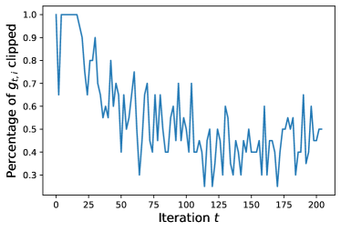
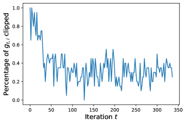
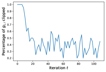
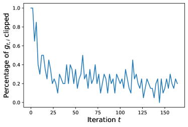
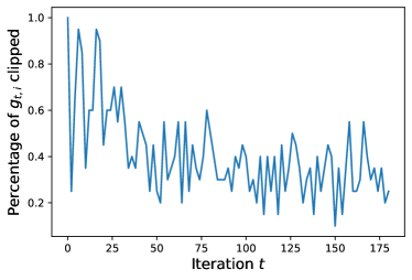
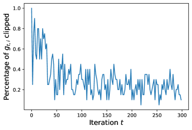
We note that for GPT2, GPT2 medium and GPT2 large, empirically in all iterations 100% of the per-sample gradients are clipped by the Abadi’s clipping, making the performance of Abadi’s clipping equivalent to AUTO-V clipping, as shown in Table 4.

H.2 Stability constant helps AUTO clipping reduce gradient norm

To corroborate our claim in Theorem 6, that the stability $\gamma$ reduces the gradient norm, we plot the actual gradient norm by iteration.

Figure 14: Gradient norm by different automatic clipping methods, on SST2 (left) and MNLI (right), trained with RoBERTa-base.

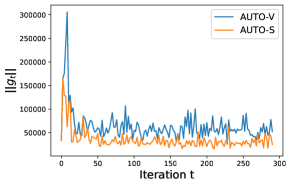
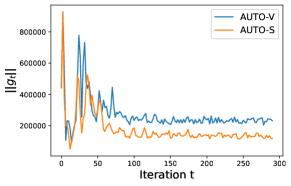
H.3 Choice of stability constant is robust

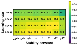
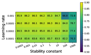
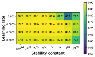
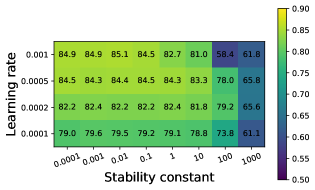
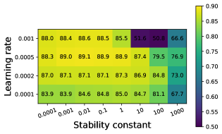
We claim in Theorem 6 that, as long as $\gamma>0$ in our automatic clipping, the asymptotic convergence rate of gradient norm is the same as that by standard non-private SGD. We plot the ablation study of learning rate and the stability constant $\gamma$ to show that it is easy to set $\gamma$: in Table 3 and Table 3, we adopt learning rate 0.0005, under which a wide range of $0.0001<\gamma<1$ gives similar accuracy. Note that the largest good $\gamma$ is 1000 times bigger than the smallest good $\gamma$.

Figure 15: Test accuracy by different stability constant $\gamma$ and learning rate $\eta$ in automatic clipping ($\epsilon=3$). Upper row: SST2 for full 3 epochs. Middle row: QNLI for full 6 epochs. Lower row: QNLI for one epoch. Trained with RoBERTa-base (left) and RoBERTa-large (right).

Appendix I Full table of GPT2 generation task on E2E dataset

This is the extended version of Table 4 on E2E dataset. The performance measures are BLEU [57], ROGUE-L [42], NIST [63], METEOR [4], and CIDEr [70] scores. Here $\epsilon$ is accounted by RDP [51], where $\epsilon=3$ corresponds to 2.68 if accounted by Gaussian DP [19, 7] or to 2.75 if accounted by numerical composition [30], and $\epsilon=8$ corresponds to 6.77 if accounted by Gaussian DP or to 7.27 if accounted by numerical composition.

	DP	GPT2	GPT2	GPT2
Metric	guarantee	large	medium
		full	full	full	full	full	LoRA	RGP	prefix	top2	retrain
		AUTO-S	AUTO-S	AUTO-S	AUTO-V	[41]	[33]	[78]	[40]	[41]	[41]
BLEU	$\epsilon=3$	64.180	63.850	61.340	61.519	61.519	58.153	58.482	47.772	25.920	15.457
	$\epsilon=8$	64.640	64.220	63.600	63.189	63.189	63.389	58.455	49.263	26.885	24.247
	non-DP	66.840	68.500	69.463	69.463	69.463	69.682	68.328	68.845	65.752	65.731
ROGUE-L	$\epsilon=3$	67.857	67.071	65.872	65.670	65.670	65.773	65.560	58.964	44.536	35.240
	$\epsilon=8$	68.968	67.533	67.073	66.429	66.429	67.525	65.030	60.730	46.421	39.951
	non-DP	70.384	71.458	71.359	71.359	71.359	71.709	68.844	70.805	68.704	68.751
NIST	$\epsilon=3$	7.937	7.106	7.071	6.697	6.697	5.463	5.775	5.249	1.510	0.376
	$\epsilon=8$	8.301	8.172	7.714	7.444	7.444	7.449	6.276	5.525	1.547	1.01
	non-DP	8.730	8.628	8.780	8.780	8.780	8.822	8.722	8.722	8.418	8.286
METEOR	$\epsilon=3$	0.403	0.387	0.387	0.384	0.384	0.370	0.331	0.363	0.197	0.113
	$\epsilon=8$	0.420	0.418	0.404	0.400	0.400	0.407	0.349	0.364	0.207	0.145
	non-DP	0.460	0.449	0.461	0.461	0.461	0.463	0.456	0.445	0.443	0.429
CIDEr	$\epsilon=3$	2.008	1.754	1.801	1.761	1.761	1.581	1.300	1.507	0.452	0.116
	$\epsilon=8$	2.163	2.081	1.938	1.919	1.919	1.948	1.496	1.569	0.499	0.281
	non-DP	2.356	2.137	2.422	2.422	2.422	2.491	2.418	2.345	2.180	2.004

Table 8: Test performance on E2E dataset with GPT2. The best two GPT2 models for each row are marked in bold.

We observe that GPT2 (163 million parameters), GPT2-medium (406 million), and GPT2-large (838 million), Table 4 trained with our automatic clipping consistently perform better in comparison to other methods. In some cases, LoRA trained with Abadi’s clipping also demonstrates strong performance and it would be interesting to see how LoRA trained with the automatic clipping will behave.

Appendix J Further experiments on CelebA dataset

In this section, we present a complete summary of accuracy results, with DP constraint or not, for the CelebA dataset. We do not apply any data-preprocessing. In the first experiment, we apply a single ResNet on the 40 labels as the multi-task/multi-label learning. In the second experiment, we apply one ResNet on one label. As expected, our automatic DP optimizers have comparable test accuracy to the Abadi’s DP optimizers, but we do not need to tune the clipping threshold for each individual task/label. We also notice that, learning different labels separately gives better accuracy than learning all labels together, though at the cost of heavier computational burden.

J.1 Multi-label classification

We apply ResNet9 as in Section G.1 on the multi-label classification task. I.e. the output layer has 40 neurons, each corresponding to one sigmoid cross-entropy loss, that are summed to a single loss and all labels are learnt jointly.

Index	Attributes	Abadi’s	AUTO-S	Abadi’s	AUTO-S	non-DP
		$\epsilon=3$	$\epsilon=3$	$\epsilon=8$	$\epsilon=8$	$\epsilon=\infty$
0	5 o Clock Shadow	90.64	90.99$\color[rgb]{0,1,0}{\uparrow}$	90.81	91.28$\color[rgb]{0,1,0}{\uparrow}$	93.33
1	Arched Eyebrows	75.15	76.31$\color[rgb]{0,1,0}{\uparrow}$	76.84	77.11$\color[rgb]{0,1,0}{\uparrow}$	81.52
2	Attractive	75.85	76.10$\color[rgb]{0,1,0}{\uparrow}$	77.50	77.74$\color[rgb]{0,1,0}{\uparrow}$	81.15
3	Bags Under Eyes	80.75	81.12$\color[rgb]{0,1,0}{\uparrow}$	82.15	82.13$\color[rgb]{1,0,0}{\downarrow}$	84.81
4	Bald	97.84	97.87$\color[rgb]{0,1,0}{\uparrow}$	98.04	97.98$\color[rgb]{1,0,0}{\downarrow}$	98.58
5	Bangs	92.71	92.68$\color[rgb]{1,0,0}{\downarrow}$	93.46	93.55$\color[rgb]{0,1,0}{\uparrow}$	95.50
6	Big Lips	67.51	67.78$\color[rgb]{0,1,0}{\uparrow}$	68.34	68.44$\color[rgb]{0,1,0}{\uparrow}$	71.33
7	Big Nose	78.01	80.23$\color[rgb]{0,1,0}{\uparrow}$	76.69	80.59$\color[rgb]{0,1,0}{\uparrow}$	83.54
8	Black Hair	81.92	80.95$\color[rgb]{1,0,0}{\downarrow}$	83.33	83.28$\color[rgb]{1,0,0}{\downarrow}$	88.55
9	Blond Hair	92.25	92.38$\color[rgb]{0,1,0}{\uparrow}$	93.52	93.09$\color[rgb]{1,0,0}{\downarrow}$	95.49
10	Blurry	94.91	94.82$\color[rgb]{1,0,0}{\downarrow}$	95.08	94.90$\color[rgb]{1,0,0}{\downarrow}$	95.78
11	Brown Hair	80.13	82.50$\color[rgb]{0,1,0}{\uparrow}$	83.74	83.89$\color[rgb]{0,1,0}{\uparrow}$	87.79
12	Bushy Eyebrows	88.06	88.23$\color[rgb]{0,1,0}{\uparrow}$	89.72	88.80$\color[rgb]{1,0,0}{\downarrow}$	92.19
13	Chubby	94.72	94.54$\color[rgb]{1,0,0}{\downarrow}$	94.54	94.50$\color[rgb]{1,0,0}{\downarrow}$	95.56
14	Double Chin	95.19	95.49$\color[rgb]{0,1,0}{\uparrow}$	95.50	95.51$\color[rgb]{0,1,0}{\uparrow}$	96.09
15	Eyeglasses	97.06	97.64$\color[rgb]{0,1,0}{\uparrow}$	98.32	98.06$\color[rgb]{1,0,0}{\downarrow}$	99.39
16	Goatee	95.68	95.45$\color[rgb]{1,0,0}{\downarrow}$	95.84	95.87$\color[rgb]{0,1,0}{\uparrow}$	97.06
17	Gray Hair	96.77	96.79$\color[rgb]{0,1,0}{\uparrow}$	97.02	97.03$\color[rgb]{0,1,0}{\uparrow}$	98.06
18	Heavy Makeup	84.96	85.70$\color[rgb]{0,1,0}{\uparrow}$	87.58	87.29$\color[rgb]{1,0,0}{\downarrow}$	90.76
19	High Cheekbones	81.46	81.42$\color[rgb]{1,0,0}{\downarrow}$	82.62	82.72$\color[rgb]{0,1,0}{\uparrow}$	86.62
20	Male	92.05	92.17$\color[rgb]{0,1,0}{\uparrow}$	93.32	93.17$\color[rgb]{1,0,0}{\downarrow}$	97.46
21	Mouth Slightly Open	86.20	86.32$\color[rgb]{0,1,0}{\uparrow}$	87.84	88.48$\color[rgb]{0,1,0}{\uparrow}$	93.07
22	Mustache	96.05	95.96$\color[rgb]{1,0,0}{\downarrow}$	96.08	95.99$\color[rgb]{1,0,0}{\downarrow}$	96.74
23	Narrow Eyes	84.90	84.78$\color[rgb]{1,0,0}{\downarrow}$	85.14	85.18$\color[rgb]{0,1,0}{\uparrow}$	86.98
24	No Beard	91.55	91.67$\color[rgb]{0,1,0}{\uparrow}$	92.29	92.45$\color[rgb]{0,1,0}{\uparrow}$	95.18
25	Oval Face	71.26	71.42$\color[rgb]{0,1,0}{\uparrow}$	71.98	71.25$\color[rgb]{1,0,0}{\downarrow}$	74.62
26	Pale Skin	96.09	96.04$\color[rgb]{1,0,0}{\downarrow}$	96.15	96.17$\color[rgb]{0,1,0}{\uparrow}$	96.93
27	Pointy Nose	70.34	72.11$\color[rgb]{0,1,0}{\uparrow}$	72.23	73.01$\color[rgb]{0,1,0}{\uparrow}$	75.68
28	Receding Hairline	91.53	91.37$\color[rgb]{1,0,0}{\downarrow}$	91.75	91.74$\color[rgb]{1,0,0}{\downarrow}$	92.87
29	Rosy Cheeks	93.26	93.02$\color[rgb]{1,0,0}{\downarrow}$	93.56	93.35$\color[rgb]{1,0,0}{\downarrow}$	94.86
30	Sideburns	96.16	96.09$\color[rgb]{1,0,0}{\downarrow}$	96.27	96.46$\color[rgb]{0,1,0}{\uparrow}$	97.44
31	Smiling	86.39	87.08$\color[rgb]{0,1,0}{\uparrow}$	88.87	88.63$\color[rgb]{1,0,0}{\downarrow}$	92.25
32	Straight Hair	76.20	77.95$\color[rgb]{0,1,0}{\uparrow}$	78.78	78.52$\color[rgb]{1,0,0}{\downarrow}$	80.66
33	Wavy Hair	70.30	71.79$\color[rgb]{0,1,0}{\uparrow}$	73.58	73.19$\color[rgb]{1,0,0}{\downarrow}$	79.15
34	Wearing Earrings	80.53	81.52$\color[rgb]{0,1,0}{\uparrow}$	82.29	82.20$\color[rgb]{1,0,0}{\downarrow}$	87.56
35	Wearing Hat	96.99	96.83$\color[rgb]{1,0,0}{\downarrow}$	97.46	97.31$\color[rgb]{1,0,0}{\downarrow}$	98.68
36	Wearing Lipstick	88.95	88.04$\color[rgb]{1,0,0}{\downarrow}$	89.87	90.72$\color[rgb]{0,1,0}{\uparrow}$	93.49
37	Wearing Necklace	84.59	85.83$\color[rgb]{0,1,0}{\uparrow}$	85.93	85.42$\color[rgb]{1,0,0}{\downarrow}$	86.61
38	Wearing Necktie	93.91	93.91–	94.43	94.08$\color[rgb]{1,0,0}{\downarrow}$	96.30
39	Young	81.35	81.21$\color[rgb]{1,0,0}{\downarrow}$	82.18	82.52$\color[rgb]{0,1,0}{\uparrow}$	87.18

Table 9: Accuracy on CelebA dataset with settings in Section G.1 from one run. The green arrow indicates AUTO-S is better than Abadi’s clipping under the same $\epsilon$; the red arrow indicates otherwise; the black bar indicates the same accuracy.

J.2 Multiple binary classification

For the second experiment, we apply ResNet9 on each label as a binary classification task. I.e. the output layer has 1 neuron and we run 40 different models for all labels separately.

Index	Attributes	Abadi’s	AUTO-S	Abadi’s	AUTO-S	non-DP
		Single	Single	Multi	Multi	Multi
		$\epsilon=8$	$\epsilon=8$	$\epsilon=8$	$\epsilon=8$	$\epsilon=\infty$
0	5 o Clock Shadow	92.15	92.29$\color[rgb]{0,1,0}{\uparrow}$	90.81	91.28$\color[rgb]{0,1,0}{\uparrow}$	93.33
1	Arched Eyebrows	81.18	80.19$\color[rgb]{1,0,0}{\downarrow}$	76.84	77.11$\color[rgb]{0,1,0}{\uparrow}$	81.52
2	Attractive	79.31	79.79$\color[rgb]{0,1,0}{\uparrow}$	77.50	77.74$\color[rgb]{0,1,0}{\uparrow}$	81.15
3	Bags Under Eyes	83.52	83.48$\color[rgb]{1,0,0}{\downarrow}$	82.15	82.13$\color[rgb]{1,0,0}{\downarrow}$	84.81
4	Bald	97.89	97.88$\color[rgb]{1,0,0}{\downarrow}$	98.04	97.98$\color[rgb]{1,0,0}{\downarrow}$	98.58
5	Bangs	94.52	94.83$\color[rgb]{0,1,0}{\uparrow}$	93.46	93.55$\color[rgb]{0,1,0}{\uparrow}$	95.50
6	Big Lips	67.32	67.53$\color[rgb]{0,1,0}{\uparrow}$	68.34	68.44$\color[rgb]{0,1,0}{\uparrow}$	71.33
7	Big Nose	82.31	82.36$\color[rgb]{0,1,0}{\uparrow}$	76.69	80.59$\color[rgb]{0,1,0}{\uparrow}$	83.54
8	Black Hair	87.08	86.93$\color[rgb]{1,0,0}{\downarrow}$	83.33	83.28$\color[rgb]{1,0,0}{\downarrow}$	88.55
9	Blond Hair	94.29	94.73$\color[rgb]{0,1,0}{\uparrow}$	93.52	93.09$\color[rgb]{1,0,0}{\downarrow}$	95.49
10	Blurry	94.95	95.20$\color[rgb]{0,1,0}{\uparrow}$	95.08	94.90$\color[rgb]{1,0,0}{\downarrow}$	95.78
11	Brown Hair	87.41	87.19$\color[rgb]{1,0,0}{\downarrow}$	83.74	83.89$\color[rgb]{0,1,0}{\uparrow}$	87.79
12	Bushy Eyebrows	91.23	91.43$\color[rgb]{0,1,0}{\uparrow}$	89.72	88.80$\color[rgb]{1,0,0}{\downarrow}$	92.19
13	Chubby	94.70	94.70–	94.54	94.50$\color[rgb]{1,0,0}{\downarrow}$	95.56
14	Double Chin	95.43	95.43–	95.50	95.51$\color[rgb]{0,1,0}{\uparrow}$	96.09
15	Eyeglasses	98.88	99.14$\color[rgb]{0,1,0}{\uparrow}$	98.32	98.06$\color[rgb]{1,0,0}{\downarrow}$	99.39
16	Goatee	96.12	96.07$\color[rgb]{1,0,0}{\downarrow}$	95.84	95.87$\color[rgb]{0,1,0}{\uparrow}$	97.06
17	Gray Hair	97.48	97.34$\color[rgb]{1,0,0}{\downarrow}$	97.02	97.03$\color[rgb]{0,1,0}{\uparrow}$	98.06
18	Heavy Makeup	88.85	88.72$\color[rgb]{1,0,0}{\downarrow}$	87.58	87.29$\color[rgb]{1,0,0}{\downarrow}$	90.76
19	High Cheekbones	85.66	85.45$\color[rgb]{1,0,0}{\downarrow}$	82.62	82.72$\color[rgb]{0,1,0}{\uparrow}$	86.62
20	Male	95.42	95.70$\color[rgb]{0,1,0}{\uparrow}$	95.53	93.17$\color[rgb]{1,0,0}{\downarrow}$	97.46
21	Mouth Slightly Open	92.67	92.74$\color[rgb]{0,1,0}{\uparrow}$	87.84	88.48$\color[rgb]{0,1,0}{\uparrow}$	93.07
22	Mustache	96.13	96.13–	96.08	95.99$\color[rgb]{1,0,0}{\downarrow}$	96.74
23	Narrow Eyes	85.13	85.13–	85.14	85.18$\color[rgb]{0,1,0}{\uparrow}$	86.98
24	No Beard	94.26	94.58$\color[rgb]{0,1,0}{\uparrow}$	92.29	92.45$\color[rgb]{0,1,0}{\uparrow}$	95.18
25	Oval Face	70.77	73.05$\color[rgb]{0,1,0}{\uparrow}$	71.98	71.25$\color[rgb]{1,0,0}{\downarrow}$	74.62
26	Pale Skin	96.38	96.34$\color[rgb]{1,0,0}{\downarrow}$	96.15	96.17$\color[rgb]{0,1,0}{\uparrow}$	96.93
27	Pointy Nose	71.48	73.37$\color[rgb]{0,1,0}{\uparrow}$	72.23	73.01$\color[rgb]{0,1,0}{\uparrow}$	75.68
28	Receding Hairline	91.51	91.51–	91.75	91.74$\color[rgb]{1,0,0}{\downarrow}$	92.87
29	Rosy Cheeks	93.26	93.35$\color[rgb]{0,1,0}{\uparrow}$	93.56	93.35$\color[rgb]{1,0,0}{\downarrow}$	94.86
30	Sideburns	96.46	96.34$\color[rgb]{1,0,0}{\downarrow}$	96.27	96.46$\color[rgb]{0,1,0}{\uparrow}$	97.44
31	Smiling	90.82	90.87$\color[rgb]{0,1,0}{\uparrow}$	88.87	88.63$\color[rgb]{1,0,0}{\downarrow}$	92.25
32	Straight Hair	79.01	79.01–	78.78	78.52$\color[rgb]{1,0,0}{\downarrow}$	80.66
33	Wavy Hair	77.55	78.83$\color[rgb]{0,1,0}{\uparrow}$	73.58	73.19$\color[rgb]{1,0,0}{\downarrow}$	79.15
34	Wearing Earrings	87.33	87.50$\color[rgb]{0,1,0}{\uparrow}$	82.29	82.20$\color[rgb]{1,0,0}{\downarrow}$	87.56
35	Wearing Hat	98.04	98.11$\color[rgb]{0,1,0}{\uparrow}$	97.46	97.31$\color[rgb]{1,0,0}{\downarrow}$	98.68
36	Wearing Lipstick	92.05	90.46$\color[rgb]{1,0,0}{\downarrow}$	89.87	90.72$\color[rgb]{0,1,0}{\uparrow}$	93.49
37	Wearing Necklace	86.21	86.21–	85.93	85.42$\color[rgb]{1,0,0}{\downarrow}$	86.61
38	Wearing Necktie	95.85	95.94$\color[rgb]{0,1,0}{\uparrow}$	94.43	94.08$\color[rgb]{1,0,0}{\downarrow}$	96.30
39	Young	85.19	84.12$\color[rgb]{1,0,0}{\downarrow}$	82.18	82.52$\color[rgb]{0,1,0}{\uparrow}$	87.18

Table 10: Accuracy on CelebA dataset with settings in Section G.1 from one run. ‘Single’ means each attribute is learned separately as a binary classification task. ‘Multi’ means all attributes are learned jointly as a multi-label classification task. The green arrow indicates AUTO-S is better than Abadi’s clipping under the same $\epsilon$ and the same task; the red arrow indicates otherwise; the black bar indicates the same accuracy.

Appendix K Code implementation of automatic clipping

Changing Abadi’s clipping to automatic clipping is easy in available codebases. One can set the clipping $R=1$ or any other constant, as explained in Theorem 1 and Theorem 2.

K.1 Opacus

For Opacus [77] version 1.1.2 (latest), we can implement the all-layer automatic clipping by changing Line 399-401 in https://github.com/pytorch/opacus/blob/main/opacus/optimizers/optimizer.py to

per_sample_clip_factor = self.max_grad_norm /(per_sample_norms + 0.01)

The per-layer automatic clipping requires changing Line 61-63 in https://github.com/pytorch/opacus/blob/main/opacus/optimizers/perlayeroptimizer.py to

per_sample_clip_factor =max_grad_norm / (per_sample_norms + 0.01)

For older version ($<1.0$, e.g. 0.15) of Opacus, we can implement the all-layer automatic clipping by changing Line 223-225 in https://github.com/pytorch/opacus/blob/v0.15.0/opacus/utils/clipping.py to

per_sample_clip_factor = self.flat_value / (norms[0] + 0.01)

or implement the per-layer automatic clipping by changing Line 301-302 in https://github.com/pytorch/opacus/blob/main/opacus/optimizers/perlayeroptimizer.py to

per_sample_clip_factor = threshold / (norm + 0.01)
clipping_factor.append(per_sample_clip_factor)

K.2 ObJAX

For ObJAX version 1.6.0 (latest), we can implement the automatic clipping in https://github.com/google/objax/blob/master/objax/privacy/dpsgd/gradient.py by changing Line 92 to

idivisor = self.l2_norm_clip / (total_grad_norm+0.01)

and changing Line 145 to

idivisor = self.l2_norm_clip/(grad_norms+0.01)

K.3 Private-transformers

To reproduce our experiments for sentence classification and table-to-text generation, we modify the ‘private-transformers’ (version 0.1.0) codebase of [41]. The modification is in https://github.com/lxuechen/private-transformers/blob/main/private_transformers/privacy_utils/privacy_engine.py, by changing Line 349 to

return self.max_grad_norm / (norm_sample + 0.01)

and Line 510-512 to

coef_sample = self.max_grad_norm * scale / (norm_sample + 0.01)

Appendix L More on related works of per-sample clipping

We discuss the difference between our work and the related (see the table below).

$C_{i}$	reference	clipping or not	convergence analysis	experiments
$\min(1,\frac{R}{||\bm{g}_{i}||})$	[1, 41]	clipping	None	CV and NLP
$\min(\frac{1}{R},\frac{1}{||\bm{g}_{i}||})$	[17]	clipping	None	CV only
$\frac{R}{||\bm{g}_{i}||}$	[16]	normalization	convex and federated setting (not per-sample)	CV only
$\frac{1}{||\bm{g}_{i}||+\gamma}$	[74]	normalization	non-convex, relaxed Lipschitz smoothness	CV and NLP
$\frac{1}{||\bm{g}_{i}||+\gamma}$	this work	normalization	non-convex, same smoothness as non-DP	CV and NLP

Table 11: Comparison between clipping functions. CV means computer vision and NLP means natural language processing. Notice that any clipping function with $R$ is not automatic and requires tuning, and that the stability constant $\gamma$ enjoys theoretical and empirical benefits.

Our work is very different to most works which do not analyze the convergence of DP deep learning in a non-convex setting, but it is very similar to [74]. However, [74] assumes a relaxed Lipschitz smootheness in place of our 5.3, where we instead assume the symmetric gradient noise. In addition, our experiments are more comprehensive, covering over 10 tasks including DP-GPT2, while [74] only experimented with 2 smaller models — ResNet20 and Roberta-base.

L.1 Clarifications

We now clarify some false or incomplete conclusion in previous literatures that apply the per-sample gradient clipping (re-parameterized or not).

1. Per-sample clipping is not robust to $R$, even with re-parameterization.

In [17, Figure 8] and our Figure 4, the accuracy of DP optimizer with Abadi’s clipping is insensitive to $R$ only if one has found a small enough region (e.g. $R\leq 1$), which takes effort to find or the accuracy will be unacceptably low out of the region. In particular, choosing $R=1$ as in [17] is not universally proper, e.g. [41] uses $R=0.1$ for language models. This dependence on tasks, datasets and optimizers means per-sample clipping still requires the expensive hyperparameter tuning.

In other words, per-sample gradient clipping is at best an approximation of per-sample gradient normalization (i.e. our AUTO-V) and should be considered as semi-automatic, whereas AUTO-V/S is fully automatic in terms of tuning $R$. Although technically we introduce a new hyperparameter $\gamma$ in the place of $R$, we claim that automatic clipping is not sensitive to $\gamma$ (our only hyperparameter) for a large range, e.g. one can multiply $\gamma$ by 10000 times, going from $\gamma=$0.001 to 10 with learning rate 0.0005 in Figure 15, and the accuracy is similar.

2. Per-sample clipping does not decouple $R$, especially for DP-Adam.

In general, $R$ is not completely decoupled from the re-parameterized per-sample clipping in [17]:

$$C_{\text{Abadi}}=\min(\frac{R}{\|\bm{g}_{i}\|},1)=R\cdot C_{\text{re-param}}=R\cdot\min(\frac{1}{\|\bm{g}_{i}\|},\frac{1}{R})$$

Given that $R$ appears in both terms on the right hand side, one can at most say "… when the clipping norm is decreased k times, the learning rate should be increased k times to maintain similar accuracy." by [38] and "… Using this update, performance becomes less sensitive to the choice of clipping norm." by [17]. In contrast, we can state that adjusting the learning rate proportionally, our AUTO-V/S maintains exactly the same accuracy and is completely insensitive to the choice of $R$.

Additionally and importantly, the understanding in [38, 17] is limited to DP-SGD (as they only experiment with the computer vision tasks), where "… the learning rate $\eta$ absorbs a factor of $R$." by [17]. As rigorously proved in Theorem 1 and Theorem 2, adaptive optimizers like Adam and AdaGrad do not absorb $R$ but rather cancel it. This is visualized in Figure 1, where the performance landscape is row-wise for DP-Adam and diagonal for DP-SGD.

3. Re-parameterized per-sample clipping unintentionally changes the weight decay.

Weight decay is a common technique used in any work that uses AdamW and in the re-parameterized trick by [17]. We can see that

$$\text{Before re-parameterization: }w_{t+1}=w_{t}-\eta\left(\frac{1}{B}\sum_{i}\min(1,\frac{R}{||g_{i}||})g_{i}+\lambda w_{t}+\frac{\sigma R}{B}N(0,I)\right)$$

$$\text{After re-parameterization: }w_{t+1}=w_{t}-\eta\left(\frac{1}{B}\sum_{i}\min(\frac{1}{R},\frac{1}{||g_{i}||})g_{i}+\frac{\lambda}{R}w_{t}+\frac{\sigma}{B}N(0,I)\right)$$

Therefore, when we move along $R$ like in [17, Figure 8], from $R=1$ to $2^{-6}$, the weight decay increases from $\lambda$ to $2^{6}\cdot\lambda$ by 64 times, which may worsen the accuracy as seen in the blue curve of [17, Figure 8]! Again, this is due to the incomplete decoupling by per-sample clipping, which is only avoided in AUTO-V/S thanks to theoretical analysis in Theorem 1 and Theorem 2.

$$\text{AUTO-V/S with weight decay: }w_{t+1} =w_{t}-\eta\left(\frac{1}{B}\sum_{i}\frac{1}{\|g_{i}\|+\gamma}g_{i}+\lambda w_{t}+\frac{\sigma}{B}\mathcal{N}(0,I)\right).$$

L.2 Connections to normalized optimisation

Variants of normalized gradient have been used in optimization [47, 53, 81, 80, 15]. These normalized optimizers are fundamentally different to our automatic optimizers, because the normalization is on mini-batch not on each sample and noise is not involved:

$$\text{NSGD: }w_{t+1} =w_{t}-\eta\left(\frac{\frac{1}{B}\sum_{i}g_{i}}{\|\frac{1}{B}\sum_{i}g_{i}\|}\right)$$

$$\text{AUTO-V: }w_{t+1} =w_{t}-\eta\left(\frac{1}{B}\sum_{i}\frac{g_{i}}{\|g_{i}\|}+\frac{\sigma}{B}\mathcal{N}(0,I)\right).$$

The main difference lies in the challenge of analyzing per-sample normalization (which is biased) and the batch-gradient normalization (which is unbiased in the direction). That is, $\frac{\frac{1}{B}\sum_{i}g_{i}}{\|\frac{1}{B}\sum_{i}g_{i}\|}$ is parallel to the mini-batch gradient $\frac{1}{B}\sum_{i}g_{i}$ but $\frac{1}{B}\sum_{i}\frac{g_{i}}{\|g_{i}\|}$ is generally not parallel to it (this conclusion also holds if the normalizaiton is replaced by the clipping). On a side note, it is interesting that Theorem 4 indeed shows although a bias is introduced by the per-sample clipping, it is not fatal to the asymptotic convergence and hence may not be a concerning matter.

References

- [1] Martin Abadi, Andy Chu, Ian Goodfellow, H Brendan McMahan, Ilya Mironov, Kunal Talwar, and Li Zhang. Deep learning with differential privacy. In Proceedings of the 2016 ACM SIGSAC conference on computer and communications security, pages 308–318, 2016.
- [2] Zeyuan Allen-Zhu. Natasha 2: Faster non-convex optimization than sgd. Advances in neural information processing systems, 31, 2018.
- [3] Galen Andrew, Om Thakkar, Brendan McMahan, and Swaroop Ramaswamy. Differentially private learning with adaptive clipping. Advances in Neural Information Processing Systems, 34, 2021.
- [4] Satanjeev Banerjee and Alon Lavie. METEOR: An automatic metric for MT evaluation with improved correlation with human judgments. In Proceedings of the ACL Workshop on Intrinsic and Extrinsic Evaluation Measures for Machine Translation and/or Summarization, pages 65–72, Ann Arbor, Michigan, June 2005. Association for Computational Linguistics.
- [5] Jeremy Bernstein, Yu-Xiang Wang, Kamyar Azizzadenesheli, and Animashree Anandkumar. signsgd: Compressed optimisation for non-convex problems. In International Conference on Machine Learning, pages 560–569. PMLR, 2018.
- [6] Léon Bottou, Frank E Curtis, and Jorge Nocedal. Optimization methods for large-scale machine learning. Siam Review, 60(2):223–311, 2018.
- [7] Zhiqi Bu, Jinshuo Dong, Qi Long, and Weijie J Su. Deep learning with gaussian differential privacy. Harvard data science review, 2020(23), 2020.
- [8] Zhiqi Bu, Sivakanth Gopi, Janardhan Kulkarni, Yin Tat Lee, Hanwen Shen, and Uthaipon Tantipongpipat. Fast and memory efficient differentially private-sgd via jl projections. Advances in Neural Information Processing Systems, 34, 2021.
- [9] Zhiqi Bu, Hua Wang, and Qi Long. On the convergence and calibration of deep learning with differential privacy. arXiv preprint arXiv:2106.07830, 2021.
- [10] Mark Bun, Cynthia Dwork, Guy N Rothblum, and Thomas Steinke. Composable and versatile privacy via truncated cdp. In Proceedings of the 50th Annual ACM SIGACT Symposium on Theory of Computing, pages 74–86, 2018.
- [11] Nicholas Carlini, Florian Tramer, Eric Wallace, Matthew Jagielski, Ariel Herbert-Voss, Katherine Lee, Adam Roberts, Tom Brown, Dawn Song, Ulfar Erlingsson, et al. Extracting training data from large language models. In 30th USENIX Security Symposium (USENIX Security 21), pages 2633–2650, 2021.
- [12] Pratik Chaudhari and Stefano Soatto. Stochastic gradient descent performs variational inference, converges to limit cycles for deep networks. In 2018 Information Theory and Applications Workshop (ITA), pages 1–10. IEEE, 2018.
- [13] Ting Chen, Simon Kornblith, Mohammad Norouzi, and Geoffrey Hinton. A simple framework for contrastive learning of visual representations. In International conference on machine learning, pages 1597–1607. PMLR, 2020.
- [14] Xiangyi Chen, Steven Z Wu, and Mingyi Hong. Understanding gradient clipping in private sgd: A geometric perspective. Advances in Neural Information Processing Systems, 33:13773–13782, 2020.
- [15] Ashok Cutkosky and Harsh Mehta. Momentum improves normalized sgd. In International conference on machine learning, pages 2260–2268. PMLR, 2020.
- [16] Rudrajit Das, Abolfazl Hashemi, Sujay Sanghavi, and Inderjit S Dhillon. On the convergence of differentially private federated learning on non-lipschitz objectives, and with normalized client updates. arXiv preprint arXiv:2106.07094, 2021.
- [17] Soham De, Leonard Berrada, Jamie Hayes, Samuel L Smith, and Borja Balle. Unlocking high-accuracy differentially private image classification through scale. arXiv preprint arXiv:2204.13650, 2022.
- [18] Jia Deng, Wei Dong, Richard Socher, Li-Jia Li, Kai Li, and Li Fei-Fei. Imagenet: A large-scale hierarchical image database. In 2009 IEEE conference on computer vision and pattern recognition, pages 248–255. Ieee, 2009.
- [19] Jinshuo Dong, Aaron Roth, and Weijie J Su. Gaussian differential privacy. Journal of the Royal Statistical Society Series B, 84(1):3–37, 2022.
- [20] Timothy Dozat. Incorporating nesterov momentum into adam. 2016.
- [21] Jian Du and Haitao Mi. Dp-fp: Differentially private forward propagation for large models. arXiv preprint arXiv:2112.14430, 2021.
- [22] John Duchi, Elad Hazan, and Yoram Singer. Adaptive subgradient methods for online learning and stochastic optimization. Journal of machine learning research, 12(7), 2011.
- [23] Ondrej Dusek, Jekaterina Novikova, and Verena Rieser. Evaluating the State-of-the-Art of End-to-End Natural Language Generation: The E2E NLG Challenge. Computer Speech & Language, 59:123–156, January 2020.
- [24] Cynthia Dwork. Differential privacy: A survey of results. In International conference on theory and applications of models of computation, pages 1–19. Springer, 2008.
- [25] Cynthia Dwork, Frank McSherry, Kobbi Nissim, and Adam Smith. Calibrating noise to sensitivity in private data analysis. In Theory of cryptography conference, pages 265–284. Springer, 2006.
- [26] Cynthia Dwork, Aaron Roth, et al. The algorithmic foundations of differential privacy. Found. Trends Theor. Comput. Sci., 9(3-4):211–407, 2014.
- [27] Saeed Ghadimi and Guanghui Lan. Stochastic first-and zeroth-order methods for nonconvex stochastic programming. SIAM Journal on Optimization, 23(4):2341–2368, 2013.
- [28] Aditya Golatkar, Alessandro Achille, Yu-Xiang Wang, Aaron Roth, Michael Kearns, and Stefano Soatto. Mixed differential privacy in computer vision. In Proceedings of the IEEE/CVF Conference on Computer Vision and Pattern Recognition, pages 8376–8386, 2022.
- [29] Ian Goodfellow, Jonathon Shlens, and Christian Szegedy. Explaining and harnessing adversarial examples. In International Conference on Learning Representations, 2015.
- [30] Sivakanth Gopi, Yin Tat Lee, and Lukas Wutschitz. Numerical composition of differential privacy. Advances in Neural Information Processing Systems, 34, 2021.
- [31] Jiyan He, Xuechen Li, Da Yu, Huishuai Zhang, Janardhan Kulkarni, Yin Tat Lee, Arturs Backurs, Nenghai Yu, and Jiang Bian. Exploring the limits of differentially private deep learning with group-wise clipping. arXiv preprint arXiv:2212.01539, 2022.
- [32] Kaiming He, Xiangyu Zhang, Shaoqing Ren, and Jian Sun. Deep residual learning for image recognition. In Proceedings of the IEEE conference on computer vision and pattern recognition, pages 770–778, 2016.
- [33] Edward J Hu, Phillip Wallis, Zeyuan Allen-Zhu, Yuanzhi Li, Shean Wang, Lu Wang, Weizhu Chen, et al. Lora: Low-rank adaptation of large language models. In International Conference on Learning Representations, 2021.
- [34] Shankar Iyer, Nikhil Dandekar, and Kornel Csernai. First quora dataset release: Question pairs, 2017.
- [35] Diederik Kingma and Jimmy Ba. Adam: A method for stochastic optimization. International Conference on Learning Representations, 12 2014.
- [36] Helena Klause, Alexander Ziller, Daniel Rueckert, Kerstin Hammernik, and Georgios Kaissis. Differentially private training of residual networks with scale normalisation. arXiv preprint arXiv:2203.00324, 2022.
- [37] Antti Koskela, Joonas Jälkö, and Antti Honkela. Computing tight differential privacy guarantees using fft. In International Conference on Artificial Intelligence and Statistics, pages 2560–2569. PMLR, 2020.
- [38] Alexey Kurakin, Steve Chien, Shuang Song, Roxana Geambasu, Andreas Terzis, and Abhradeep Thakurta. Toward training at imagenet scale with differential privacy. arXiv preprint arXiv:2201.12328, 2022.
- [39] Quentin Lhoest, Albert Villanova del Moral, Yacine Jernite, Abhishek Thakur, Patrick von Platen, Suraj Patil, Julien Chaumond, Mariama Drame, Julien Plu, Lewis Tunstall, Joe Davison, Mario Sasko, Gunjan Chhablani, Bhavitvya Malik, Simon Brandeis, Teven Le Scao, Victor Sanh, Canwen Xu, Nicolas Patry, Angelina McMillan-Major, Philipp Schmid, Sylvain Gugger, Clément Delangue, Théo Matussière, Lysandre Debut, Stas Bekman, Pierric Cistac, Thibault Goehringer, Victor Mustar, François Lagunas, Alexander Rush, and Thomas Wolf. Datasets: A community library for natural language processing. In Proceedings of the 2021 Conference on Empirical Methods in Natural Language Processing: System Demonstrations, pages 175–184, Online and Punta Cana, Dominican Republic, November 2021. Association for Computational Linguistics.
- [40] Xiang Lisa Li and Percy Liang. Prefix-tuning: Optimizing continuous prompts for generation. In Proceedings of the 59th Annual Meeting of the Association for Computational Linguistics and the 11th International Joint Conference on Natural Language Processing (Volume 1: Long Papers), pages 4582–4597, 2021.
- [41] Xuechen Li, Florian Tramer, Percy Liang, and Tatsunori Hashimoto. Large language models can be strong differentially private learners. In International Conference on Learning Representations, 2021.
- [42] Chin-Yew Lin. ROUGE: A package for automatic evaluation of summaries. In Text Summarization Branches Out, pages 74–81, Barcelona, Spain, July 2004. Association for Computational Linguistics.
- [43] Liyuan Liu, Haoming Jiang, Pengcheng He, Weizhu Chen, Xiaodong Liu, Jianfeng Gao, and Jiawei Han. On the variance of the adaptive learning rate and beyond. In International Conference on Learning Representations, 2019.
- [44] Yinhan Liu, Myle Ott, Naman Goyal, Jingfei Du, Mandar Joshi, Danqi Chen, Omer Levy, Mike Lewis, Luke Zettlemoyer, and Veselin Stoyanov. Roberta: A robustly optimized bert pretraining approach. arXiv preprint arXiv:1907.11692, 2019.
- [45] Ziwei Liu, Ping Luo, Xiaogang Wang, and Xiaoou Tang. Deep learning face attributes in the wild. In Proceedings of International Conference on Computer Vision (ICCV), December 2015.
- [46] Ilya Loshchilov and Frank Hutter. Decoupled weight decay regularization. In International Conference on Learning Representations, 2018.
- [47] Danilo P Mandic. A generalized normalized gradient descent algorithm. IEEE signal processing letters, 11(2):115–118, 2004.
- [48] Stephan Mandt, Matthew D Hoffman, and David M Blei. Stochastic gradient descent as approximate bayesian inference. Journal of Machine Learning Research, 18:1–35, 2017.
- [49] H Brendan McMahan, Daniel Ramage, Kunal Talwar, and Li Zhang. Learning differentially private recurrent language models. In International Conference on Learning Representations, 2018.
- [50] Harsh Mehta, Abhradeep Thakurta, Alexey Kurakin, and Ashok Cutkosky. Large scale transfer learning for differentially private image classification. arXiv preprint arXiv:2205.02973, 2022.
- [51] Ilya Mironov. Rényi differential privacy. In 2017 IEEE 30th computer security foundations symposium (CSF), pages 263–275. IEEE, 2017.
- [52] Diganta Misra. Mish: A self regularized non-monotonic activation function. BMVC 2020, 2019.
- [53] Ryan Murray, Brian Swenson, and Soummya Kar. Revisiting normalized gradient descent: Fast evasion of saddle points. IEEE Transactions on Automatic Control, 64(11):4818–4824, 2019.
- [54] Yurii E Nesterov. A method for solving the convex programming problem with convergence rate o (1/k^ 2). In Dokl. akad. nauk Sssr, volume 269, pages 543–547, 1983.
- [55] Nicolas Papernot and Thomas Steinke. Hyperparameter tuning with renyi differential privacy. In International Conference on Learning Representations, 2021.
- [56] Nicolas Papernot, Abhradeep Thakurta, Shuang Song, Steve Chien, and Úlfar Erlingsson. Tempered sigmoid activations for deep learning with differential privacy. In Proceedings of the AAAI Conference on Artificial Intelligence, volume 35, pages 9312–9321, 2021.
- [57] Kishore Papineni, Salim Roukos, Todd Ward, and Wei-Jing Zhu. Bleu: A method for automatic evaluation of machine translation. In Proceedings of the 40th Annual Meeting on Association for Computational Linguistics, ACL ’02, page 311–318, USA, 2002. Association for Computational Linguistics.
- [58] Venkatadheeraj Pichapati, Ananda Theertha Suresh, Felix X Yu, Sashank J Reddi, and Sanjiv Kumar. Adaclip: Adaptive clipping for private sgd. arXiv preprint arXiv:1908.07643, 2019.
- [59] Boris T Polyak. Some methods of speeding up the convergence of iteration methods. Ussr computational mathematics and mathematical physics, 4(5):1–17, 1964.
- [60] Boris T Polyak and Anatoli B Juditsky. Acceleration of stochastic approximation by averaging. SIAM journal on control and optimization, 30(4):838–855, 1992.
- [61] Siyuan Qiao, Huiyu Wang, Chenxi Liu, Wei Shen, and Alan Yuille. Micro-batch training with batch-channel normalization and weight standardization. arXiv preprint arXiv:1903.10520, 2019.
- [62] Pranav Rajpurkar, Jian Zhang, Konstantin Lopyrev, and Percy Liang. Squad: 100, 000+ questions for machine comprehension of text. In EMNLP, 2016.
- [63] Seyed Omid Sadjadi, Timothee Kheyrkhah, Audrey Tong, Craig S Greenberg, Douglas A Reynolds, Elliot Singer, Lisa P Mason, Jaime Hernandez-Cordero, et al. The 2017 nist language recognition evaluation. In Odyssey, pages 82–89, 2018.
- [64] Ali Shahin Shamsabadi and Nicolas Papernot. Losing less: A loss for differentially private deep learning. 2021.
- [65] Reza Shokri, Marco Stronati, Congzheng Song, and Vitaly Shmatikov. Membership inference attacks against machine learning models. In 2017 IEEE symposium on security and privacy (SP), pages 3–18. IEEE, 2017.
- [66] Samuel L Smith, Pieter-Jan Kindermans, Chris Ying, and Quoc V Le. Don’t decay the learning rate, increase the batch size. In International Conference on Learning Representations, 2018.
- [67] Richard Socher, Alex Perelygin, Jean Wu, Jason Chuang, Christopher D Manning, Andrew Ng, and Christopher Potts. Recursive deep models for semantic compositionality over a sentiment treebank. In Proceedings of the 2013 conference on empirical methods in natural language processing, pages 1631–1642, 2013.
- [68] Florian Tramer and Dan Boneh. Differentially private learning needs better features (or much more data). In International Conference on Learning Representations, 2020.
- [69] Ashish Vaswani, Noam Shazeer, Niki Parmar, Jakob Uszkoreit, Llion Jones, Aidan N Gomez, Łukasz Kaiser, and Illia Polosukhin. Attention is all you need. Advances in neural information processing systems, 30, 2017.
- [70] Ramakrishna Vedantam, C Lawrence Zitnick, and Devi Parikh. Cider: Consensus-based image description evaluation. In Proceedings of the IEEE conference on computer vision and pattern recognition, pages 4566–4575, 2015.
- [71] Yu-Xiang Wang, Borja Balle, and Shiva Prasad Kasiviswanathan. Subsampled rényi differential privacy and analytical moments accountant. In International Conference on Artificial Intelligence and Statistics, pages 1226–1235. PMLR, 2019.
- [72] Adina Williams, Nikita Nangia, and Samuel Bowman. A broad-coverage challenge corpus for sentence understanding through inference. In Proceedings of the 2018 Conference of the North American Chapter of the Association for Computational Linguistics: Human Language Technologies, Volume 1 (Long Papers), pages 1112–1122. Association for Computational Linguistics, 2018.
- [73] Zeke Xie, Issei Sato, and Masashi Sugiyama. A diffusion theory for deep learning dynamics: Stochastic gradient descent exponentially favors flat minima. In International Conference on Learning Representations, 2020.
- [74] Xiaodong Yang, Huishuai Zhang, Wei Chen, and Tie-Yan Liu. Normalized/clipped sgd with perturbation for differentially private non-convex optimization. arXiv preprint arXiv:2206.13033, 2022.
- [75] Yang You, Igor Gitman, and Boris Ginsburg. Scaling sgd batch size to 32k for imagenet training. arXiv preprint arXiv:1708.03888, 6(12):6, 2017.
- [76] Yang You, Jing Li, Sashank Reddi, Jonathan Hseu, Sanjiv Kumar, Srinadh Bhojanapalli, Xiaodan Song, James Demmel, Kurt Keutzer, and Cho-Jui Hsieh. Large batch optimization for deep learning: Training bert in 76 minutes. In International Conference on Learning Representations, 2020.
- [77] Ashkan Yousefpour, Igor Shilov, Alexandre Sablayrolles, Davide Testuggine, Karthik Prasad, Mani Malek, John Nguyen, Sayan Ghosh, Akash Bharadwaj, Jessica Zhao, Graham Cormode, and Ilya Mironov. Opacus: User-friendly differential privacy library in PyTorch. arXiv preprint arXiv:2109.12298, 2021.
- [78] Da Yu, Huishuai Zhang, Wei Chen, Jian Yin, and Tie-Yan Liu. Large scale private learning via low-rank reparametrization. In International Conference on Machine Learning, pages 12208–12218. PMLR, 2021.
- [79] Matthew D Zeiler. Adadelta: an adaptive learning rate method. arXiv preprint arXiv:1212.5701, 2012.
- [80] Shen-Yi Zhao, Yin-Peng Xie, and Wu-Jun Li. Stochastic normalized gradient descent with momentum for large batch training. arXiv preprint arXiv:2007.13985, 2020.
- [81] Shen-Yi Zhao, Yin-Peng Xie, and Wu-Jun Li. On the convergence and improvement of stochastic normalized gradient descent. Science China Information Sciences, 64:1–13, 2021.
- [82] Yuqing Zhu, Jinshuo Dong, and Yu-Xiang Wang. Optimal accounting of differential privacy via characteristic function. In International Conference on Artificial Intelligence and Statistics, pages 4782–4817. PMLR, 2022.